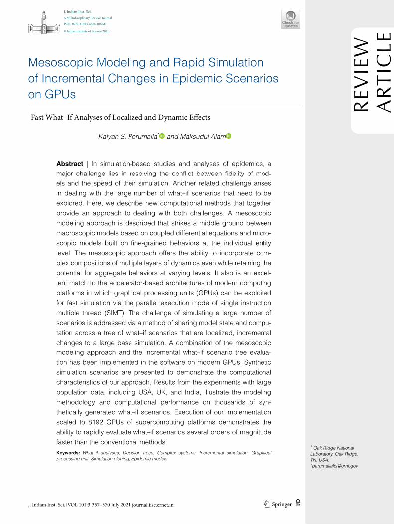
1 3J. Indian Inst. Sci. | VOL 101:3 | 357–370 July 2021 | journal.iisc.ernet.in

Mesoscopic Modeling and Rapid Simulation of Incremental Changes in Epidemic Scenarios on GPUs

Fast What–If Analyses of Localized and Dynamic Effects

Kalyan S. Perumalla* and Maksudul Alam

J. Indian Inst. Sci.

A Multidisciplinary Reviews Journal

ISSN: 0970-4140 Coden-JIISAD

Abstract | In simulation-based studies and analyses of epidemics, a major challenge lies in resolving the conflict between fidelity of mod-els and the speed of their simulation. Another related challenge arises in dealing with the large number of what–if scenarios that need to be explored. Here, we describe new computational methods that together provide an approach to dealing with both challenges. A mesoscopic modeling approach is described that strikes a middle ground between macroscopic models based on coupled differential equations and micro-scopic models built on fine-grained behaviors at the individual entity level. The mesoscopic approach offers the ability to incorporate com-plex compositions of multiple layers of dynamics even while retaining the potential for aggregate behaviors at varying levels. It also is an excel-lent match to the accelerator-based architectures of modern computing platforms in which graphical processing units (GPUs) can be exploited for fast simulation via the parallel execution mode of single instruction multiple thread (SIMT). The challenge of simulating a large number of scenarios is addressed via a method of sharing model state and compu-tation across a tree of what–if scenarios that are localized, incremental changes to a large base simulation. A combination of the mesoscopic modeling approach and the incremental what–if scenario tree evalua-tion has been implemented in the software on modern GPUs. Synthetic simulation scenarios are presented to demonstrate the computational characteristics of our approach. Results from the experiments with large population data, including USA, UK, and India, illustrate the modeling methodology and computational performance on thousands of syn-thetically generated what–if scenarios. Execution of our implementation scaled to 8192 GPUs of supercomputing platforms demonstrates the ability to rapidly evaluate what–if scenarios several orders of magnitude faster than the conventional methods.Keywords: What–if analyses, Decision trees, Complex systems, Incremental simulation, Graphical processing unit, Simulation cloning, Epidemic models

REV

IEW

A

RT

ICLE

© Indian Institute of Science 2021.

1 Oak Ridge National Laboratory, Oak Ridge, TN, USA. *perumallaks@ornl.gov

358

K. S. Perumalla, M. Alam

1 3 J. Indian Inst. Sci.| VOL 101:3 | 357–370 July 2021 | journal.iisc.ernet.in

1 IntroductionThe tremendous significance of analyzing and understanding the dynamics of epidemics is now abundantly clear in light of not only many major disease outbreaks of the past, but also with the most pronounced and consequential effects of COVID-19 worldwide2,25,26. Computer-based simulations are used for many purposes to deal with this problem, including prediction, con-firmation, validation, exploration, enhancing our understanding, establishing limits, and so on. This brings greater emphasis to the need for creating the next generation of computational approaches to modeling and simulating epidemic dynamics12,13,19,23. This includes the need for advances in computer-based modeling capabili-ties by which the most important elements and behaviors are accurately composed and captured. It is now public knowledge that the epidemic-influenced world is one of the most complex systems humans have encountered so far, pos-ing difficulties to the researchers in balancing the mutually opposing factors of model fidelity, simulation speed, and real-time evaluation. On a positive note, the challenge is also an excel-lent opportunity for the scientific community to explore, uncover, and offer newer concepts, tech-nologies, and solutions to this class of problems and also consequently carry the advances to other domains as well for similar advancements.

1.1 MotivationOne of the advancements that the domain can use is in new modeling and simulation approaches that preserve the primary benefits of both the extremities, namely, macroscopic and microscopic modeling, while largely overcoming their shortcomings. The next advancement relates to the thorny problem faced by every modeling and simulation effort for complex systems: how can we effectively explore the vast parameter space of what–if analyses in which a large num-ber of possibilities on the near-term time hori-zon are explored quickly as small, incremental variations of scenarios over the current, large state of the complex system6. The scenarios to be explored become numerous due to the multitude of factors at play, which include location-specific effects, behavioral effects, intervention measures, and so on2,9,28. On one hand, massive simulations of microscopic models cannot typically be run in large numbers of scenarios. On the other hand, macroscopic models are easily run, but the num-ber of parameters is typically not as high as with higher resolution models1,3,8.

Apart from the number of scenarios, there is an additional challenge that is commonly faced, namely the problem of meeting real-time consid-erations. When simulation is used to explore the effects even as the situation is evolving, there is the additional pressure to evaluate as many sce-narios as possible in a given amount of real time, so that well-informed decisions can be made quickly18–20.

These considerations present new questions with respect to modeling and simulation tech-nology4,13. Can we have a flexible middle ground between the two extremes of macroscopic and microscopic models? Can the scalability of mac-roscopic models be approached even while new models of dynamics are incorporated in arbitrary compositions? How can we modify a simulation scenario on the fly and create new what–if scenar-ios, even while the state trajectories in the original scenario continue to be evaluated over time, con-currently with the incremental what–if scenarios spawned from the original scenario? How can we let a scenario continue to run while sharing its state with the slightly changed what–if scenarios? Can we let the what–if scenarios reuse much of the original epidemic scenario, even as both con-tinue to evolve in simulation time?

1.2 ContributionsIn this paper, we focus on presenting new com-putational concepts and possibilities for next generation of epidemic simulations, by providing advancements on both aspects: fast base simula-tion and rapid exploration of what–if trees over the base simulation. As a middle ground, meso-scopic models represent an appropriate class in which the resolution and number of parameters are sufficiently high to capture a fair amount of phenomenological complexity, and thus warrant a good sweep of scenario parameters to improve the accuracy and assurance from simulation-based studies. Therefore, a mesoscopic simulation approach is described that offers the potential to serve as a continuum from macroscopic to microscopic levels, whose configurations can be customized based on data availability, desired modeling accuracy, targeted level of behavioral detail, and other such factors. Building over this mesoscopic framework, an incremental simula-tion approach based on what–if tree evolution is presented that offers new scaling capabilities that were not possible before in rapidly simu-lating thousands or millions of incrementally varied scenarios over a large domain of a base simulation2,25,26. The mesoscopic model can be

359

Mesoscopic Modeling and Rapid Simulation

1 3J. Indian Inst. Sci. | VOL 101:3 | 357–370 July 2021 | journal.iisc.ernet.in

used in the incremental what–if tree evalua-tion on state-of-the-art accelerated computing platforms including supercomputers that offer thousands of GPUs, and effectively exploit the single-instruction-multiple-data (SIMD) mode of high-performance parallel computing. The two approaches together form the basis for new computational ways of tackling the modeling and simulation problem in epidemic studies and deci-sion systems.

Our focus here is on presenting novel compu-tational approaches for fast simulation of large-scale population sizes and for rapid exploration of massive numbers of what–if scenarios. As a result, the epidemic dynamics do not specifically represent any particular configurations from real-life situations, although the general trends are validated to conform to the expect evolution from standard propagation models. The goal is to present the new computational methodolo-gies that are now available from this research for domain scientists to explore and exploit towards real-life studies. Therefore, the approach and fea-sibility results presented here in scalable mod-eling and fast scenario exploration are envisioned to provide a leap in the simulation capabilities for analyzing epidemics and other complex systems.

A major challenge is the number of param-eters, scenarios, and conditions at play. It is nearly impossible to run a simulation for every combi-nation of parameters for scenarios30. Traditional simulations11 serve well with experiment design techniques to address the problem of sampling the state space. For significant advances, how-ever, new paradigms need to be developed to advance the epidemiological simulation technol-ogy. Methods such as factorial experiment design and Latin square sampling are commonly used, along with recent methods for uncertainty quan-tification, but there is little support for incremen-tal changes to large scenarios, and insufficient methodology to deal with large what–if trees in conjunction with mesoscopic simulations in an efficient manner. Compounding the problem, the additional dimension of real-time simulation and decision-making places a higher expectation of rapid evaluation of dynamically created scenar-ios. The what–if scenarios come in sequences and branches, forming a tree of evaluations. Also, the branches that need to be evaluated can be exoge-nous, based on new external inputs to the simula-tion based on evolving ground truth or influx of data. The updates may also appear in the form of internal simulation state-based conditions (e.g., a new event with a certain probability will arise only when the state satisfies certain conditions),

which are difficult to schedule a priori in a con-ventional experiment design.

1.3 OrganizationThe rest of the paper is organized as follows. Our mesoscopic approach to the large, complex systems of epidemics is presented in Sect. 2. The computational framework to enable rapid explo-ration of massive trees of incremental what–if scenarios is described in Sect. 3. This is followed in Sect. 4 by a performance study using compu-tational experiments on three basic country-scale models, with sequential (one node) performance as well as small-scale and large-scale parallel exe-cution on up to 8192 GPUs. The paper is summa-rized and future work identified in Sect. 5.

2 �Mesoscopic�Approach�to Large,�Complex�Systems

2.1 Conceptual FrameworkThe modeling spectrum for any large, com-plex system in general spans the space between two extremes with respect to the level of detail included per interacting entity in the system. In the epidemic case, the most numerous entities in the system are the individuals who are targets of the disease. Therefore, the two extremes for epi-demic modeling span the two ends with respect to the level of detail captured in the model per individual. When the individuals are merely rep-resented as counts of certain bins such as the total number of susceptible individuals and the number of infected individuals, such a model is a macroscopic model7. In a macroscopic model, there is little additional identity or distinguishing factor on an individual basis, but only aggregates are represented and tracked. In the other extreme, when each individual entity is demarcated and explicit state of its own that is tracked separately from that of other entities, such a model is a microscopic model10. Recently, mesoscale mod-eling has been used at local level or regional level for modeling and validating COVID-19 at the county level15.

Mesoscopic modeling can provide a good trade-off between fidelity and speed of simu-lation. At the right level of population density (number of individuals per grid cell), it can cap-ture the dynamics of microscopic models with differential equations while providing the ease of composing many effects that can be varied at the level of each grid cell. At higher grid sizes, the population density can be reduced even further, potentially down to a few dozen people per grid cell. This can either be specified as a specialized,

360

K. S. Perumalla, M. Alam

1 3 J. Indian Inst. Sci.| VOL 101:3 | 357–370 July 2021 | journal.iisc.ernet.in

individual-level model or an aggregate, difference equation-based approximation to the high-reso-lution microscopic model.

2.2 Mapping the Model to SIMD GridFor the highest resolution data partitioning of population to grid cells, it may be possible to change the mesoscopic model to a microscopic, individual-level model for more accurately cap-turing the dynamics. For example, in the case of UK, it is seen that the average population size per grid cell indeed approaches a single individual when the grid size is 8192 × 8192. The trans-formation of mesoscopic-to-microscopic model opens new research directions as future work.

Each cell in the grid represents an aggregate of population. Therefore, every grid cell executes the differential equations presented in the subse-quent sections for the epidemic model, infection model, spatial model, and inter-entity interaction model. This makes the mesoscopic approach a strict superset of the macroscopic approach. Con-sequently, it is possible to take any macroscopic model and incorporate it into the mesoscopic model.

The power of this grid-based mesoscopic approach comes from its excellent alignment with the fast SIMD processing capabilities of mod-ern GPUs. This match of the model to the GPUs offers three important benefits:

1. This model can be executed on any desk-top machine of a researcher or practitioner, making fast, large-scale simulations acces-sible to many important users without sig-nificant additional investments for compu-tational support.

2. The use of the GPU also makes it possible to offer interactive animations of the dynam-ics even as the simulations are executed. Since the GPU is also a rendering device, the latency between computation and visualiza-tion is minimized. Moreover, the visualiza-tion software layer is extremely light due to the native support provided by most GPU vendors, including standardized interfaces such as OpenGL.

3. In the case of practitioners or researchers who have access to large parallel comput-ing platforms, the GPU-based mesoscopic approach is perfectly suited to exploit the parallel system. Many large computational clusters, cloud computing platforms, or even

supercomputers, offer GPU-based nodes. In fact, the top supercomputers of the world are currently ranked at the top exclusively because of their hardware design that is heavily GPU-based.

2.3 Epidemic ModelWe illustrate our mesoscopic modeling approach using the parameters of an Ebola epidemic model, although the methodology is general and applica-ble to many other epidemics. For experimenta-tion purposes, we use a few parameters and fitted values for an epidemic (Ebloa 2014) model22. The parameter values are shown in Table 1. We solve the system of linear equations using initial condi-tions with values corresponding to the countries. In particular, we assume that for the countries considered in this work, the initial exposed popu-lations are both 10% of the aggregate ones.

Note that this configuration and settings are chosen only to exercise the computational frame-work, and hence are not meant as actual validated studies. Because any scenario-specific values can be varied by the user, the system is general pur-pose in nature and not limited to any specific model or components. Our focus here is limited to presenting the novel approach to modeling and simulation on current accelerated computing architectures.

2.4 Infection ModelWe use a general metapopulation-based suscep-tible-exposed-infectious-recovered (SEIR) epi-demic model5. We assume that the environment under consideration is divided into L location patches, which are geographic regions. Each patch is considered to be homogeneous and divided into four compartments where individuals are classified as:

  – S: Susceptible individuals, who can be infected;

Table 1: Model parameters and fitted values for an Ebola epidemic model.

Parameter Region 1 Region 2

Contact rate β 0.128 0.16

Incubation period 1/δ 10 days 12 days

Infectious Period 1/γ 10.38 days 13.31 days

361

Mesoscopic Modeling and Rapid Simulation

1 3J. Indian Inst. Sci. | VOL 101:3 | 357–370 July 2021 | journal.iisc.ernet.in

 – E: Exposed individuals, who have been infected but not yet infectious;

 – I: Infectious cases in the community, who are capable of transmitting the disease;

 – R: Individuals removed from the chain of transmission (cured or dead and buried).

The number of people of each compartment in path i at some time t is denoted by Si(t) , Ei(t) , Ii(t) , and Ri(t) , respectively for i = 1, 2, . . . , L . The total number of people in patch i is denoted by Ni(t) = Si(t)+ Ei(t)+ Ii(t)+ Ri(t) . The population will be constant during the outbreak.

The model takes into consideration the num-ber of people infected due to direct contact with an infected individual and the number of people infected due to direct contact with latent individ-uals: β SI

N . The individuals in the latent stage will eventually show the symptoms of the disease and enter into the infectious stage. This is denoted as δE , where δ is the per-capita infectious rate. In that case, 1

δ becomes the average time for a latent

individual to become infectious. The recovery rate is denoted by γ I , where γ is the per-capita recovery rate.

2.5 Spatial Mobility ModelWe also model the behavior that individuals travel between the patches. The rates of travel of individuals between any two patches can be made to depend on the disease state. The disease states of individuals do not change during travel. The simplest travel pattern per time step is move-ment from any given grid cell to its immediate Moore neighborhood5,14,21. However, this can be customized with another mapping array for arbi-trary connectivity, especially for modeling the non-local effects of air travel and long rail/high-way-based interactions.

2.6 Consolidated ModelWhen the SEIR infection model is integrated with the spatial mobility model, each grid cell updates its counts based on the combined terms of com-partments as described next.

Let mSij , m

Eij , m

Iij , and mR

ij denote the travel rate from patch i to patch j of susceptible, exposed, infective, and recovered individuals, respectively, where mS

ii = mEii = mI

ii = mRii = 0 . The travel

rates among all the patches can be represented by matrices MS = [mS

ij] , ME = [mE

ij ] , MI = [mI

ij] , and MR = [mR

ij] where 1 ≤ i, j ≤ L

This set of equations is mapped to each grid ele-ment. At every time step, the grid elements are updated concurrently in an SIMD fashion. Global statistics are computed periodically for visualiza-tion and output generation purposes.

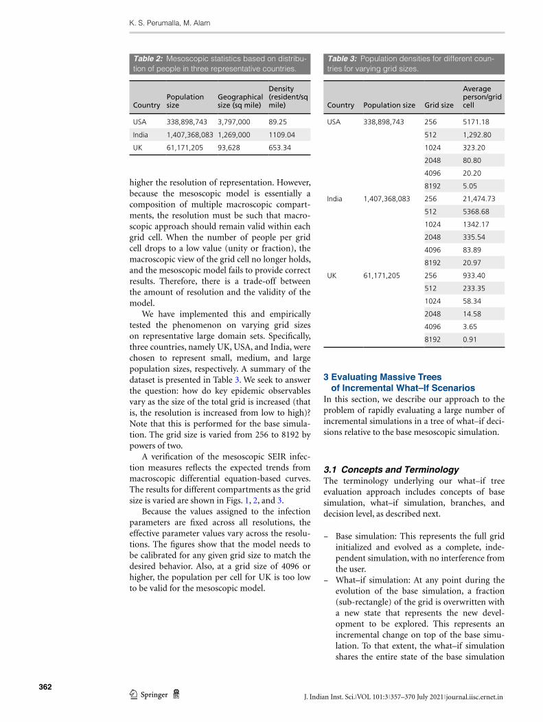
2.7 Data SourcesThe geographical population data per country is collected from the WorldPop dataset27 using the methods described in17. The population datasets are available in GeoTIFF format in 100 m and 1 km resolutions. We used the GDAL (Geospa-tial Data Abstraction Library) package to parse the dataset and extract the population counts per location patch. The data are used to gener-ate intermediate population files per country for various grid sizes. We used grid sizes of 256, 512, 1024, 2048, 4096, and 8192 in the experiments. We used three different countries of varying area, density, and population counts: UK, USA, and India. A summary of the dataset is presented in Table 2.

Similar data sources can be used for pre-processing and reformatted to fit the mesoscale model. For large data sets, the pre-processing itself can be parallelized to reduce the amount of data preparation time. However, this needs to be done only once for each set of initial conditions. Typically, these input data do not change too fre-quently (typically, once or twice a year), which makes the pre-processing a small, fixed cost for the mesoscale approach.

2.8 Grid Size and Model FidelityGiven a specific geographic domain and its popu-lation distribution, they can be mapped to a grid of desired size. Thus, for any given population size, the greater the size of the grid to which the population is mapped, the smaller is the num-ber of people per grid cell, and therefore, the

(1)

dSi

dt= −β

SiIi

Ni+

L∑

j=1

(

mSijSj −mS

ijSi

)

dEi

dt= β

SiIi

Ni− δEi +

L∑

j=1

(

mEijEj −mE

ijEi

)

dIi

dt= δEi − δIi +

L∑

j=1

(

mIijIj −mI

ijIi

)

dRi

dt= δIi +

L∑

j=1

(

mRijRj −mR

ijRi

)

.

362

K. S. Perumalla, M. Alam

1 3 J. Indian Inst. Sci.| VOL 101:3 | 357–370 July 2021 | journal.iisc.ernet.in

higher the resolution of representation. However, because the mesoscopic model is essentially a composition of multiple macroscopic compart-ments, the resolution must be such that macro-scopic approach should remain valid within each grid cell. When the number of people per grid cell drops to a low value (unity or fraction), the macroscopic view of the grid cell no longer holds, and the mesoscopic model fails to provide correct results. Therefore, there is a trade-off between the amount of resolution and the validity of the model.

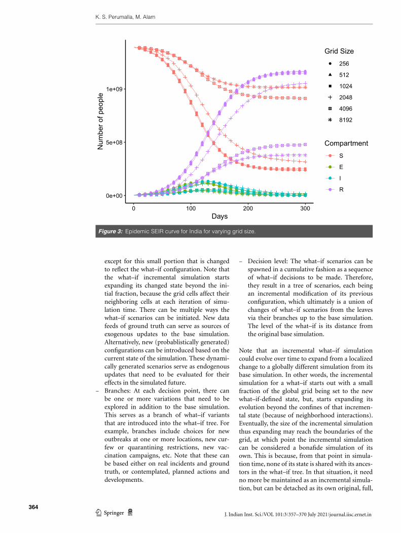
We have implemented this and empirically tested the phenomenon on varying grid sizes on representative large domain sets. Specifically, three countries, namely UK, USA, and India, were chosen to represent small, medium, and large population sizes, respectively. A summary of the dataset is presented in Table 3. We seek to answer the question: how do key epidemic observables vary as the size of the total grid is increased (that is, the resolution is increased from low to high)? Note that this is performed for the base simula-tion. The grid size is varied from 256 to 8192 by powers of two.

A verification of the mesoscopic SEIR infec-tion measures reflects the expected trends from macroscopic differential equation-based curves. The results for different compartments as the grid size is varied are shown in Figs. 1, 2, and 3.

Because the values assigned to the infection parameters are fixed across all resolutions, the effective parameter values vary across the resolu-tions. The figures show that the model needs to be calibrated for any given grid size to match the desired behavior. Also, at a grid size of 4096 or higher, the population per cell for UK is too low to be valid for the mesoscopic model.

3 �Evaluating�Massive�Trees�of Incremental�What–If�Scenarios

In this section, we describe our approach to the problem of rapidly evaluating a large number of incremental simulations in a tree of what–if deci-sions relative to the base mesoscopic simulation.

3.1 Concepts and TerminologyThe terminology underlying our what–if tree evaluation approach includes concepts of base simulation, what–if simulation, branches, and decision level, as described next.

  – Base simulation: This represents the full grid initialized and evolved as a complete, inde-pendent simulation, with no interference from the user.

 – What–if simulation: At any point during the evolution of the base simulation, a fraction (sub-rectangle) of the grid is overwritten with a new state that represents the new devel-opment to be explored. This represents an incremental change on top of the base simu-lation. To that extent, the what–if simulation shares the entire state of the base simulation

Table 2: Mesoscopic statistics based on distribu-tion of people in three representative countries.

CountryPopulation size

Geographical size (sq mile)

Density (resident/sq mile)

USA 338,898,743 3,797,000 89.25

India 1,407,368,083 1,269,000 1109.04

UK 61,171,205 93,628 653.34

Table 3: Population densities for different coun-tries for varying grid sizes.

Country Population size Grid size

Average person/grid cell

USA 338,898,743 256 5171.18

512 1,292.80

1024 323.20

2048 80.80

4096 20.20

8192 5.05

India 1,407,368,083 256 21,474.73

512 5368.68

1024 1342.17

2048 335.54

4096 83.89

8192 20.97

UK 61,171,205 256 933.40

512 233.35

1024 58.34

2048 14.58

4096 3.65

8192 0.91

363

Mesoscopic Modeling and Rapid Simulation

1 3J. Indian Inst. Sci. | VOL 101:3 | 357–370 July 2021 | journal.iisc.ernet.in

0e+00

1e+08

2e+08

3e+08

0 100 200 300Days

Num

ber o

f peo

ple

Grid Size

256

512

1024

2048

4096

8192

Compartment

S

E

I

R

Figure 1: Epidemic SEIR curve for USA for varying grid size.

0e+00

2e+07

4e+07

6e+07

0 100 200 300Days

Num

ber o

f peo

ple

Grid Size

256

512

1024

2048

4096

8192

Compartment

S

E

I

R

Figure 2: Epidemic SEIR curve for UK for varying grid size.

364

K. S. Perumalla, M. Alam

1 3 J. Indian Inst. Sci.| VOL 101:3 | 357–370 July 2021 | journal.iisc.ernet.in

except for this small portion that is changed to reflect the what–if configuration. Note that the what–if incremental simulation starts expanding its changed state beyond the ini-tial fraction, because the grid cells affect their neighboring cells at each iteration of simu-lation time. There can be multiple ways the what–if scenarios can be initiated. New data feeds of ground truth can serve as sources of exogenous updates to the base simulation. Alternatively, new (probablistically generated) configurations can be introduced based on the current state of the simulation. These dynami-cally generated scenarios serve as endogenous updates that need to be evaluated for their effects in the simulated future.

 – Branches: At each decision point, there can be one or more variations that need to be explored in addition to the base simulation. This serves as a branch of what–if variants that are introduced into the what–if tree. For example, branches include choices for new outbreaks at one or more locations, new cur-few or quarantining restrictions, new vac-cination campaigns, etc. Note that these can be based either on real incidents and ground truth, or contemplated, planned actions and developments.

 – Decision level: The what–if scenarios can be spawned in a cumulative fashion as a sequence of what–if decisions to be made. Therefore, they result in a tree of scenarios, each being an incremental modification of its previous configuration, which ultimately is a union of changes of what–if scenarios from the leaves via their branches up to the base simulation. The level of the what–if is its distance from the original base simulation.

Note that an incremental what–if simulation could evolve over time to expand from a localized change to a globally different simulation from its base simulation. In other words, the incremental simulation for a what–if starts out with a small fraction of the global grid being set to the new what–if-defined state, but, starts expanding its evolution beyond the confines of that incremen-tal state (because of neighborhood interactions). Eventually, the size of the incremental simulation thus expanding may reach the boundaries of the grid, at which point the incremental simulation can be considered a bonafide simulation of its own. This is because, from that point in simula-tion time, none of its state is shared with its ances-tors in the what–if tree. In that situation, it need no more be maintained as an incremental simula-tion, but can be detached as its own original, full,

0e+00

5e+08

1e+09

0 100 200 300Days

Num

ber o

f peo

ple

Grid Size

256

512

1024

2048

4096

8192

Compartment

S

E

I

R

Figure 3: Epidemic SEIR curve for India for varying grid size.

365

Mesoscopic Modeling and Rapid Simulation

1 3J. Indian Inst. Sci. | VOL 101:3 | 357–370 July 2021 | journal.iisc.ernet.in

base simulation in its own right, as though it was started with its own initial conditions.

3.2 Epidemic ScenariosTo study the impacts of various factors during the epidemic spread, we consider several well-studied scenarios. To evaluate the impact, a combination of these scenarios need to be tested16,24. Further-more, the scenarios are also dependent on the type of geographical areas, such as cities, rural areas, mountains, rivers, etc. We present a brief overview of the scenarios considered in this paper (Figs. 4, 5, 6).

  – Outbreak Sometimes during an epidemic out-break, some spatial regions become hot spot of epidemic outbreak. The geography and demography of those regions play an impor-tant role in understanding the control mecha-nism.

 – Spatial quarantine During an epidemic out-break in a region, sometimes, travel restric-

tions have to be applied to control the spread of diseases. The effectiveness of a quaran-tine policy depends on the spatial movement properties, such as inter-cell transportation modes and associated delays. To more accu-rately model all transportation modes such as air travel, the size of the what–if sub-region may need to be expanded to include all cells in the region between the origins and desti-nations of travel. In this paper, we restrict the movement of individuals from and to a quar-antined zone.

 – Hospitalization Many disease models include hospitalization as an intervention. We can introduce the variable Q to denote the infec-tious population being hospitalized, and the variable α to denote the rate of hospitaliza-tion22. We assume that the hospitalized indi-viduals share the same recovery probability with the normal infectious ones, but do not infect any exposed individual or susceptible one. With this approach, the base SEIR model is modified to include what–if scenarios for hospitalization as follows:

 –

(2)

dSi

dt= −

β

γSi(1− α)Ii +

L∑

j=1

(

mSijSj −mS

ijSi

)

dEi

dt=

β

γSi(1− α)Ii −

δ

γEi +

L∑

j=1

(

mEijEj −mE

ijEi

)

dIi

dt=

δ

γEi − Ii +

L∑

j=1

(

mIijIj −mI

ijIi

)

dRi

dt= Ii +

L∑

j=1

(

mRijRj −mR

ijRi

)

dQi

dt= αIi +

L∑

j=1

(

mQij Qj −m

Qij Qi

)

.

Figure 4: Snapshot of an illustrative, working vis-ualization of a what–if tree for USA.

Figure 5: Snapshot of an illustrative, working vis-ualization of a what–if tree for UK.

Figure 6: Snapshot of an illustrative, working vis-ualization of a what–if tree for India.

366

K. S. Perumalla, M. Alam

1 3 J. Indian Inst. Sci.| VOL 101:3 | 357–370 July 2021 | journal.iisc.ernet.in

 – Vaccination In the vaccination scenario, we apply vaccination to the susceptible indi-viduals to become immune to the disease. To model vaccination, we can introduce another variable V(t) to be the number of individuals who have been vaccinated22. We let the vacci-nation rate be given as a function of time by η . Thus, η is the number of individuals being vaccinated per unit time at time t. With this additional variant, the base SEIR model is modified to include what–if scenarios for vaccination as follows (this addition can be cumulative, together with the hospitalization what–if addition mentioned previously):

 –

 – Logistics To tackle an epidemic disease, quick delivery of medical supplies and hospitali-zation are crucial. However, these might be delayed due to various forms of social and geographical factors. This aspect could poten-tially be separately modeled or included in the base SEIR model by changing the rate of movement of individuals in a region.

4 �Computational�ExperimentsIn the following computational experiments for a performance study, we use India geography and population data as the test case, with a grid size of 2048× 2048 . The experiments are run on a single computational node for a baseline sequential per-formance, and also on parallel computing plat-form with several GPUs. Two what–if scenario trees are used: a small scale what–if tree with 30,000 incremental simulation scenarios, and a large-scale what–if tree with tree size of approxi-mately 350,000 scenarios.

(3)

dSi

dt= −β

SiIi

Ni− η +

L∑

j=1

(

mSijSj −mS

ijSi

)

dEi

dt= β

SiIi

Ni− δEi +

L∑

j=1

(

mEijEj −mE

ijEi

)

dIi

dt= δEi − δIi +

L∑

j=1

(

mIijIj −mI

ijIi

)

dRi

dt= δIi +

L∑

j=1

(

mRijRj −mR

ijRi

)

dVi

dt= η +

L∑

j=1

(

mVij Vj −mV

ij Vi

)

.

4.1 Performance Experiment Configurations

4.1.1 �Hardware�and SoftwareWe used a server with an NVIDIA Tesla V100 GPU with 16 GB RAM and Intel(R) Xeon(R) Silver 4110 CPU with 256 GB of host memory. The underlying operating system was UBUNTU 20.04. We used C++ for the software and CUDA 10.0 for the GPU.

For the large-scale parallel runs, we used a supercomputing system to conduct the multi-node experiments. The supercomputing system consists of 18,688 compute nodes, a total of 710 TB system memory, and Cray’s high-performance Gemini network. Each node hosts a 16-core AMD Opteron processor with 32 GB of host memory and an NVIDIA Tesla K20X GPU. Each GPU contains 2688 CUDA cores with 6 GB of device memory. The supercomputing system is based on CUDA 7.0 for the GPU, and a vendor-supplied native implementation of the Message Passing Interface (MPI) for inter-processor communica-tion and synchronization.

4.1.2  Performance ParametersThe experimental runs are conducted for a num-ber of simulation time steps to perform a suffi-cient mixture and reach of model dynamics. We used three key variables to spawn new what–if (incremental) simulation runs: (i) the fraction � of the domain affected that defines each new what–if simulation; (ii) the number of what–if scenarios m per decision sequence, and the num-ber of decisions k in sequence. We vary these parameters to evaluate the runtime performance of the system, using a value of � = 10−3 on each spatial dimension.

The spatial grid dimension W ×H with width W and height H of all our simulation experi-ments is set to 2048× 2048 . Larger dimensions result in higher resolutions and larger domains, for which what–if simulation would perform even better. For this grid size and � = 10−3 , each what–if scenario’s initial dimensions as √2048× 2048× 10−3 ≈ 64 . Hence, each

what–if simulation starts with an incrementally changed domain size of 64 × 64 , which will be modified with scenario-specific spatial data (e.g., new infections centered at the chosen location). In the experiments regarding performance evalu-ation, we used the country data for India.

The simulation model tracks the propagation dynamics based on the SEIR model specified in Sect. 2. The incremental simulations are spawned based on a variety of what–if scenarios, such as

367

Mesoscopic Modeling and Rapid Simulation

1 3J. Indian Inst. Sci. | VOL 101:3 | 357–370 July 2021 | journal.iisc.ernet.in

new outbreaks (grids with increased infected count), quarantines (restricted spatial move-ment), vaccination (reducing susceptible counts), and hospitalization (increasing recovered counts).

4.1.3  Performance MetricsAs the measure of computational effectiveness of our what–if tree evaluation framework, we use a notion of speed-up that is different from the concept of parallel speed-up traditionally used in parallel computing. In parallel computing, the (strong scaling) speed-up is the factor of reduc-tion in total computational time when multiple processors are used, relative to the time taken when only one processor is used. Here, we use a different notion, because the parallel speed-up is not applicable.

Whether one processor is used or multiple processors are used, the total time taken by the traditional simulation techniques to complete M what–if scenarios is M × TC , where TC is the time taken to complete one simulation. Note that, in normal simulation approaches, each what–if scenario essentially becomes a full simulation of its own. In our approach, only the base simula-tion is by default a full simulation, but the what–if scenarios are only incremental in nature, so

consume time to simulate only a fraction � of the original domain. Therefore, the time taken by our framework is significantly less than that of nor-mal (replicated) simulations for each what–if sce-nario. A more detailed analysis of this complexity is available in our previous work29. Based on this notion, the speed-up is defined as the factor of reduction in time using our what–if incremental scenario approach compared to fully replicated runs. Note that the savings from experiment design methods apply equally to both traditional replication approach as well as to our approach, because any scenarios that can be avoided using some such design can be equally applied to our framework as well. As such, this is a robust meas-ure with respect to comparing scenario evalu-ation via full simulation versus our what–if tree evaluation method.

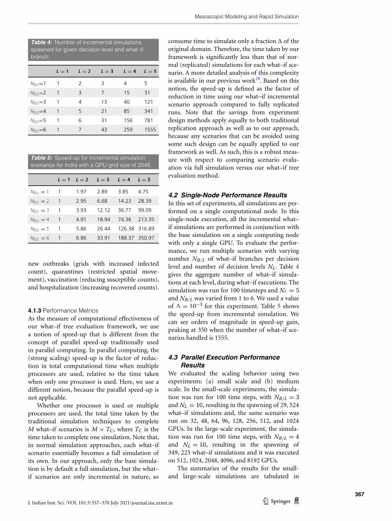
4.2 Single‑Node Performance ResultsIn this set of experiments, all simulations are per-formed on a single computational node. In this single-node execution, all the incremental what–if simulations are performed in conjunction with the base simulation on a single computing node with only a single GPU. To evaluate the perfor-mance, we run multiple scenarios with varying number NB/L of what–if branches per decision level and number of decision levels NL . Table 4 gives the aggregate number of what–if simula-tions at each level, during what–if executions. The simulation was run for 100 timesteps and NL = 5 and NB/L was varied from 1 to 6. We used a value of � = 10−3 for this experiment. Table 5 shows the speed-up from incremental simulation. We can see orders of magnitude in speed-up gain, peaking at 350 when the number of what–if sce-narios handled is 1555.

4.3 Parallel Execution Performance Results

We evaluated the scaling behavior using two experiments: (a) small scale and (b) medium scale. In the small-scale experiments, the simula-tion was run for 100 time steps, with NB/L = 3 and NL = 10 , resulting in the spawning of 29, 524 what–if simulations and, the same scenario was run on 32, 48, 64, 96, 128, 256, 512, and 1024 GPUs. In the large-scale experiment, the simula-tion was run for 100 time steps, with NB/L = 4 and NL = 10 , resulting in the spawning of 349, 225 what–if simulations and it was executed on 512, 1024, 2048, 4096, and 8192 GPUs.

The summaries of the results for the small- and large-scale simulations are tabulated in

Table 4: Number of incremental simulations spawned for given decision level and what–if branch.

L = 1 L = 2 L = 3 L = 4 L = 5

NB/L=1 1 2 3 4 5

NB/L=2 1 3 7 15 31

NB/L=3 1 4 13 40 121

NB/L=4 1 5 21 85 341

NB/L=5 1 6 31 156 781

NB/L=6 1 7 43 259 1555

Table 5: Speed-up for incremental simulation scenarios for India with a GPU grid size of 2048.

L = 1 L = 2 L = 3 L = 4 L = 5

NB/L = 1 1 1.97 2.89 3.85 4.75

NB/L = 2 1 2.95 6.68 14.23 28.39

NB/L = 3 1 3.93 12.12 36.77 99.09

NB/L = 4 1 4.91 18.94 74.36 213.35

NB/L = 5 1 5.86 26.44 126.38 316.89

NB/L = 6 1 6.86 33.91 188.37 350.97

368

K. S. Perumalla, M. Alam

1 3 J. Indian Inst. Sci.| VOL 101:3 | 357–370 July 2021 | journal.iisc.ernet.in

Tables 6 and 7, respectively. From the experimen-tal results, we can observe that the performance gain increases significantly with an increase of the number of nodes. Using up to 8192 nodes (GPUs), we can achieve a performance gain of approximately 75 K for approximately 350 K what–if simulations.

5 �Summary�and Future�WorkA mesoscale modeling approach is presented that appears suitable for modeling epidemics at large scales for first-order metrics, and well suited for exploiting the GPU platforms. We have also pre-sented a framework for generating and evaluating massive what–if scenarios, scalable from single machine to large supercomputing platforms.

It is now conceivable to rapidly evaluate mil-lions of what–if scenarios to adequately cover the parameter space and aid informed deci-sion-making in real time in evolving epidemics. The mesoscopic modeling approach presented here provides an effective way to exploit the

computational power of GPU hardware tech-nology. In some of the largest experiments, the parallel computational runs show the feasibility to utilize thousands of GPUs to explore what–if trees containing many hundreds of thousands of decision sequences in a matter of minutes. The results presented here represent some of the larg-est and fastest what–if simulations reported in the literature. In the largest case, nearly 350,000 what–if scenarios were executed on 8192 GPUs in about 2 min of wall-clock time. The same system is also usable on commodity desktop comput-ers for local and regional-scale simulation and analyses.

To use this model for a given geographical population density and grid size, the parameters need to be calibrated to maintain the right bal-ance of macroscopic versus microscopic level of models. As shown in Sect. 2, the exact global counts of SEIR compartments are depend-ent on the grid size and constants used in the model. This needs to be studied to provide the mathematical methodology needed to partition a macroscopic model into multiple sub-mac-roscopic models, so that they can be mapped to the grid. Another class of shortcomings of our approach lie in the mapping from the geographi-cal domain to the grid. Since the representation is a direct mapping, domains with contiguous land will perform better, whereas gaps in inhabi-tation on the land or presence of water bodies or other geographical separations will waste the grid cells in the GPU memory and computation. Another shortcoming is the availability of accu-rate data to initialize the simulation state in terms of the mesoscopic grid. Overall, there are multi-ple factors that need to be addressed before our approach can be readily used by actual decision-makers or practitioners. For instance, verification, validation, and accreditation processes will need to be undertaken to customize it for real-life use. Accordingly, our focus in this paper has been to first present the computational advancement that the mesoscopic representation provides and showing the potential for evaluating massive trees of what–if scenarios as incremental simulations executed on state-of-the-art GPU-based comput-ing platforms.

Publisher’s�Note Springer Nature remains neutral with regard to jurisdictional claims in published maps and insti-tutional affiliations.

Table 6: Experiments with small what–if tree with 29,524 incremental simulation scenarios.

# of GPUs Run time (s) Speed-up

1 (Base simulation only)

25.57 1.00

32 1471.81 512.98

48 762.554 990.11

64 545.523 1384.01

96 387.765 1947.08

128 329.704 2289.97

256 171.523 4401.81

512 138.404 5455.13

1024 103.879 7268.18

Table 7: Experiments with large what–if tree with 349,225 incremental simulation scenarios.

# of GPUs Runtime (s) Speedup

1 (Base simulation only)

25.57 1.00

512 1110.89 8046.10

1024 783.26 11411.72

2048 251.52 35537.55

4096 194.86 45870.77

8192 120.08 74435.86

369

Mesoscopic Modeling and Rapid Simulation

1 3J. Indian Inst. Sci. | VOL 101:3 | 357–370 July 2021 | journal.iisc.ernet.in

AcknowledgementsThis manuscript has been authored by UT-Battelle, LLC under Contract No. DE-AC05-00OR22725 with the U.S. Department of Energy. The United States Government retains and the publisher, by accepting the article for publication, acknowledges that the United States Govern-ment retains a non-exclusive, paid-up, irrevoca-ble, worldwide license to publish or reproduce the published form of this manuscript, or allow others to do so, for United States Government purposes. The Department of Energy will pro-vide public access to these results of federally sponsored research in accordance with the DOE Public Access Plan (http:// energy. gov/ downl oads/ doe- public- access- plan).

Declarations

Conflict�of�interest The authors declare that they have no conflict of interest.

Received: 13 April 2021 Accepted: 6 July 2021

Published online: 3 August 2021

References 1. Adiga A, Dubhashi D, Lewis B, Marathe M, Venkatra-

manan S, Vullikanti A (2020) Mathematical mod-

els for Covid-19 pandemic: a comparative analysis. J

Indian Inst Sci 100:793–807. https:// doi. org/ 10. 1007/

s41745- 020- 00200-6

2. Adiga A, Wang L, Sadilek A, Tendulkar A, Venkatramanan

S, Vullikanti A, Aggarwal G, Talekar A, Ben X, Chen J,

Lewis B, Swarup S, Tambe M, Marathe M (2020) Inter-

play of global multi-scale human mobility, social distanc-

ing, government interventions, and covid-19 dynamics.

medRxiv. https:// doi. org/ 10. 1101/ 2020. 06. 05. 20123 760

3. Adiga A, Wang L, Hurt B, Peddireddy A, Porebski P, Ven-

katramanan S, Lewis B, Marathe M (2021) All models are

useful: Bayesian ensembling for robust high resolution

covid-19 forecasting. medRxiv. https:// doi. org/ 10. 1101/

2021. 03. 12. 21253 495

4. Ajelli M, Gonçalves B, Balcan D, Colizza V, Hu H,

Ramasco JJ, Merler S, Vespignani A (2010) Comparing

large-scale computational approaches to epidemic mode-

ling: agent-based versus structured metapopulation mod-

els. BMC Infect Dis 10(1):1–13

5. Arino J, Van den Driessche P (2006) Metapopulation epi-

demic models. a survey. Fields Inst Commun 48:1–13

6. Bradley E, Marathe M, Moses M, Gropp WD, Lopresti D

(2020) Pandemic informatics: preparation, robustness,

and resilience; Vaccine distribution, logistics, and prior-

itization; and Variants of concern. arXiv: 2012. 09300

7. Brauer F (2008) Compartmental models in epidemiol-

ogy. In: Mathematical epidemiology. Springer, pp 19–79

8. Calvetti D, Hoover AP, Rose J, Somersalo E (2020) Metap-

opulation network models for understanding, predicting,

and managing the coronavirus disease covid-19. Front

Phys 8:261

9. Chang S, Wilson ML, Lewis B, Mehrab Z, Dudakiya KK,

Pierson E, Koh PW, Gerardin J, Redbird B, Grusky D,

Marathe M, Leskovec J (2021) Supporting covid-19 pol-

icy response with large-scale mobility-based modeling.

medRxiv. https:// doi. org/ 10. 1101/ 2021. 03. 20. 21254 022

10. Eubank S, Guclu H, Kumar VA, Marathe MV, Srini-

vasan A, Toroczkai Z, Wang N (2004) Modelling disease

outbreaks in realistic urban social networks. Nature

429(6988):180–184

11. Fujimoto RM (2000) Parallel and distributed simulation

systems. Wiley-Interscience, New York

12. Gauvin L, Panisson A, Barrat A, Cattuto C (2015) Reveal-

ing latent factors of temporal networks for mesoscale

intervention in epidemic spread. arXiv: 15010 2758

13. Hemmert KS, Bair R, Bhatele A, Groves T, Hammond SD,

Levenhagen MJ, Mubarak M, Pakin S, Ross R, Wilke JJ,

Georgakoudis G (2019) System-level architecture simula-

tion for exascale: challenges and opportunities. https://

www. osti. gov/ biblio/ 16392 11

14. Kelly MR Jr, Tien JH, Eisenberg MC, Lenhart S (2016)

The impact of spatial arrangements on epidemic dis-

ease dynamics and intervention strategies. J Biol Dyn

10(1):222–249

15. Kergaßner A, Burkhardt C, Lippold D, Kergaßner M,

Pflug L, Budday D, Steinmann P, Budday S (2020) Mem-

ory-based meso-scale modeling of covid-19: county-

resolved timelines in Germany. Comput Mech. https://

doi. org/ 10. 1007/ s00466- 020- 01883-5

16. Liu S, Poccia S, Candan KS, Chowell G, Sapino ML

(2016) epiDMS: data management and analytics for deci-

sion-making from epidemic spread simulation ensem-

bles. J Infect Dis 214(4):S427–S432. https:// doi. org/ 10.

1093/ infdis/ jiw305

17. Lloyd CT, Chamberlain H, Kerr D, Yetman G, Pistolesi

L, Stevens FR, Gaughan AE, Nieves JJ, Hornby G, Mac-

Manus K, Sinha P, Bondarenko M, Sorichetta A, Tatem AJ

(2019) Global spatio-temporally harmonised datasets for

producing high-resolution gridded population distribu-

tion datasets. Big Earth Data 3(2):108–139. https:// doi.

org/ 10. 1080/ 20964 471. 2019. 16251 51

18. López L, Rodo X (2021) A modified Seir model to pre-

dict the covid-19 outbreak in Spain and Italy: simulating

control scenarios and multi-scale epidemics. Results Phys

21:103746

19. Minutoli M, Sambaturu P, Halappanavar M, Tumeo A,

Kalyanaraman A, Vullikanti A (2020) Preempt: scalable

epidemic interventions using submodular optimization

on multi-gpu systems. In: 2020 SC20: international con-

ference for high performance computing, storage and

370

K. S. Perumalla, M. Alam

1 3 J. Indian Inst. Sci.| VOL 101:3 | 357–370 July 2021 | journal.iisc.ernet.in

analysis (SC). IEEE Computer Society, Networking, pp

765–779

20. Mishra S, Steen R, Gerbase A, Lo YR, Boily MC (2012)

Impact of high-risk sex and focused interventions in

heterosexual hiv epidemics: a systematic review of math-

ematical models. PLoS One 7(11):e50691

21. Ni S, Weng W (2009) Impact of travel patterns on epi-

demic dynamics in heterogeneous spatial metapopula-

tion networks. Phys Rev E 79(1):016111

22. Ouyang X, Son S, Yu K (2015) Modeling the spread of

ebola. Mathematical contest in modeling. https:// sites.

math. washi ngton. edu/ ~morrow/ mcm/ mcm15/ 38725

paper. pdf

23. Perumalla KS, Seal SK (2012) Discrete event modeling

and massively parallel execution of epidemic outbreak

phenomena. Simulation 88(7):768–783

24. Rivers CM, Lofgren ET, Marathe M, Eubank S, Lewis BL

(2014) Modeling the impact of interventions on an epi-

demic of Ebola in Sierra Leone and Liberia. PLoS Curr.

https:// doi. org/ 10. 1371/ curre nts. outbr eaks. 4d41f e5d6c

05e9d f30dd ce33c 66d08 4c

25. Singer G, Marudi M (2020) Ordinal decision-tree-based

ensemble approaches: the case of controlling the daily

local growth rate of the covid-19 epidemic. Entropy.

https:// doi. org/ 10. 3390/ e2208 0871

26. St-Onge G, Thibeault V, Allard A, Dubé LJ, Hébert-

Dufresne L (2021) Social confinement and mesoscopic

localization of epidemics on networks. Phys Rev Lett

126(9):098301

27. WorldPop (2021) Population counts. https:// www. world

pop. org/ geoda ta/ listi ng? id= 29

28. Wu N, Ben X, Green B, Rough K, Venkatramanan S,

Marathe M, Eastham P, Sadilek A, O’Banion S (2020)

Predicting onset of covid-19 with mobility-augmented

seir model. medRxiv. https:// doi. org/ 10. 1101/ 2020. 07. 27.

20159 996

29. Yoginath SB, Perumalla KS (2018) Scalable cloning on

large-scale gpu platforms with application to time-

stepped simulations on grids. ACM Trans Model Comput

Simul 28(1):5:1–5:26. https:// doi. org/ 10. 1145/ 31586 69

30. Zhang T, Lees M, Kwoh CK, Fu X, Lee GKK, Goh RSM

(2012) A contact-network-based simulation model for

evaluating interventions under what-if scenarios in epi-

demic. In: Proceedings of the 2012 winter simulation

conference (WSC). IEEE, pp 1–12

Kalyan S. Perumalla is a Distinguished Research Staff Member at the Oak Ridge National Laboratory (ORNL, a U.S. Depart-ment of Energy laboratory) in the Com-puter Science and Mathematics Division and is a Joint Full Professor in the School of

Industrial and Systems Engineering at the University of Tennessee, Knoxville. Dr. Perumalla also holds appoint-ments as Adjunct Professor in the School of Computational Sciences and Engineering at the Georgia Institute of Tech-nology and in the Department of Electrical and Computer Engineering at the University of Nebraska-Lincoln. He also serves on the SpecialInterest Group Governing Board of the Association for Computing Machinery (ACM) as the elected chair for ACM Special Interest Group in Simulation

(SIGSIM). Prior to his research career at ORNL since 2005, he held full-time research appointments at the Georgia Institute of Technology. He also served as Fellow of the Institute of Advanced Study at Durham University, UK, and as member of the National Academies’ Technical Advisory Boards for the U.S. Army Research Laboratory.

Maksudul Alam is a Research Staff Mem-ber at the Oak Ridge National Laboratory in the Computer Science and Mathematics Division. Prior to his research career at ORNL, he received his PhD from the Virginia Polytechnic and State University (Virginia

Tech) and completed apost-doctoral term at ORNL.