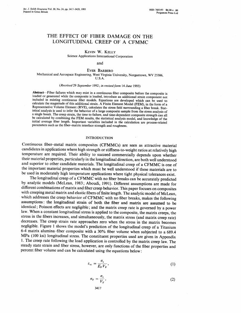
Int. J. Solids Structures Vol. 30, No. 24, pp. 3417-3429, 1993Printed in Great Britain

0020-7683/93 $6.00 + .00Pergamon Press Ltd

THE EFFECT OF FIBER DAMAGE ON THELONGITUDINAL CREEP OF A CFMMC

KEVIN W. KELLYScience Applications International Corporation

and

EVER BARBEROMechanical and Aerospace Engineering, West Virginia University, Norgantown, WV 25506,

U.S.A.

(Received 29 September 1992; in revised/orm 14 June 1993)

Abstract-Fiber failures which may exist in a continuous fiber· composite before the .composite isloaded or generated while the composite is loaded, introduce an additional strain component notincluded in existing continuous fiber models. Equations are developed which can be used tocalculate the magnitude of this additional strain. A Finite Element Model (FEM), in the form of aRepresentative Volume Element (RVE) , calculates the stress field surrounding a fiber break. Stat­istical analysis is used to infer the behavior of a large composite sample from the stress analysis ofa single break. The creep strain, the time to failure, and time-dependent composite strength can allbe calculated by combining the FEM results, the statistical analysis model, and knowledge of theinitial average fiber length. Important variables included in the calculation are process-relatedparameters such as the fiber-matrix interface strength and roughness.

INTRODUCTION

Continuous fiber-metal matrix composites (CFMMCs) are seen as attractive materialcandidates in applications where high strength or stiffness-to-weight ratios at relatively hightemperature are required. Their ability to succeed commercially depends upon whethertheir material properties, particularly in the longitudinal direction, are both well understoodand superior to other candidate materials. The longitudinal creep of a CFMMC is one ofthe important material properties which must be well understood if these materials are tobe used in moderately high temperature applications where tight physical tolerances exist.

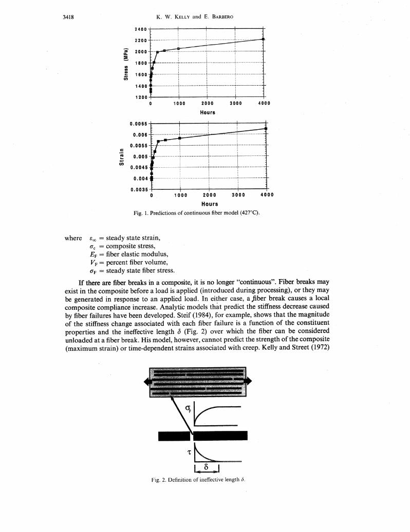
The longitudinal creep of a CFMMC with no fiber breaks can be accurately predictedby analytic models (McLean, 1983; Aboudi, 1991). Different assumptions are made fordifferent combinations ofmatrix an~ fiber creep behavior. This paper focuses on compositeswith creeping metal matrix and elastic fibers offinite length. The analytic model ofMcLean,which addresses the creep behavior of CFMMC with no fiber breaks, makes the followingassumptions: the longitudinal strain of both the fiber and matrix are assumed to beidentical; Poissori effects are negligible; and the matrix creep rate is governed by a powerlaw. When a constant longitudinal stress is applied to the composite, the matrix creeps, thestress in the fibers increases, and simultaneously, the matrix stress (and matrix creep rate)decreases. The creep strain rate approaches zero when the stress in the matrix becomesnegligible. Figure 1 shows the model's prediction of the longitudinal creep of a Titanium6-4 matrix alumina-fiber composite with a 300/0 fiber volume when subjected to a 689.4MPa (lOOksi) longitudinal stress. The constituent properties used are given in Appendix1. The creep rate following the load application is controlled by the matrix creep law. Thesteady state strain and fiber stress, however, are only functions of the fiber properties andpercent fiber volume and can be calculated using the equations below:

(1)

(2)

3417

3418

2400

2200

as 20000-e1800

tntn~ 1600en

1400

K. W. KELLY and E. BARBERO

..--------~~..-------

~l

I

1200o 1000 2000

Hours

3000 4000

0.0065

0.006

0.0055 ...cca 0.005..-C/)

0.0045

0.004

0.00350 1000 2000 3000 4000

Hours

Fig. 1. Predictions of continuous fiber model (427°C).

where Goo = steady state strain,(Jc = composite stress,EF = fiber elastic modulus,VF = percent fiber volume,(JF = steady state fiber stress.

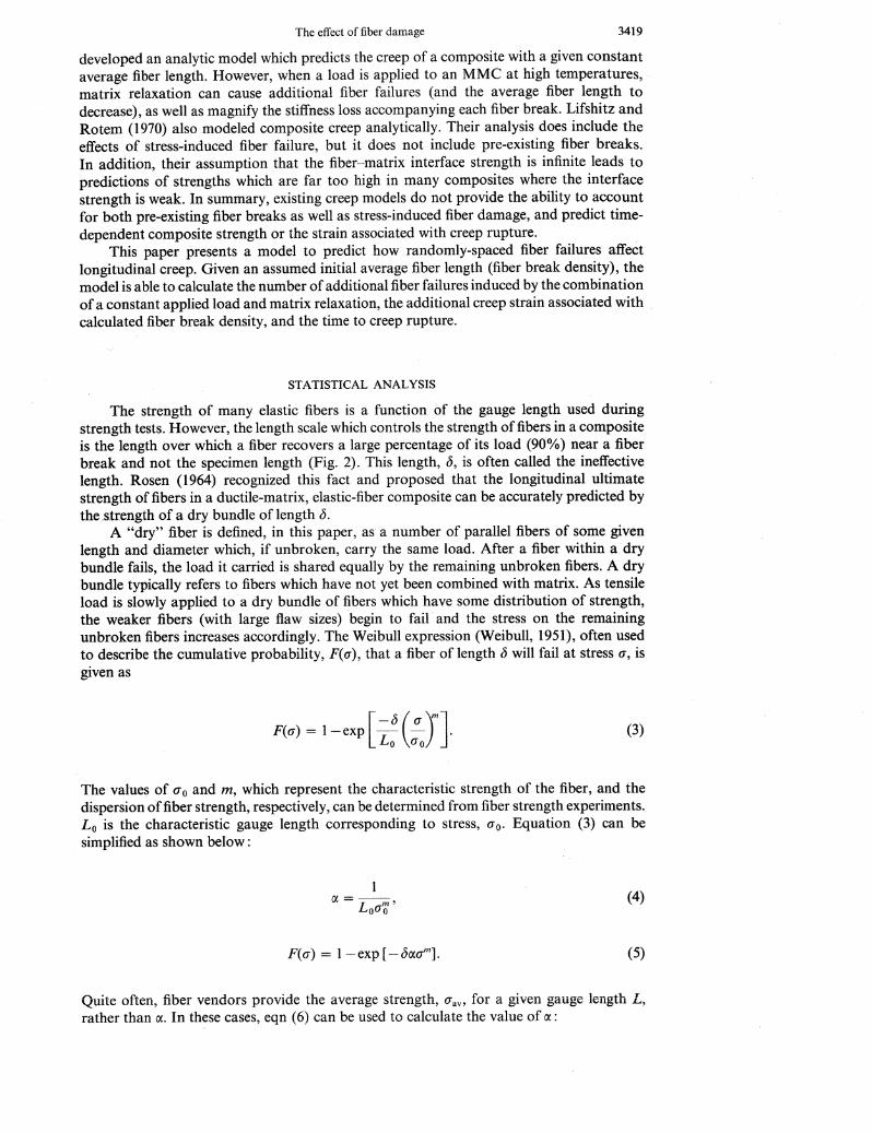
If there are fiber breaks in a composite, it is no longer "continuous". Fiber breaks mayexist in the composite before a load is applied (introduced during processing), or they maybe generated in response to an applied load. In either case, a fiber break causes a localcomposite compliance increase. Analytic models that predict the stiffness decrease causedby fiber failures have been developed. Steif (1984), for example, shows that the magnitudeof the stiffness change associated with each fiber failure is a function of the constituentproperties and the ineffective length b (Fig. 2) over which the fiber can be consideredunloaded at a fiber break. His model, however, cannot predict the strength of the composite(maximum strain) or time-dependent strains associated with creep. Kelly and Street (1972)

Fig. 2. Definition of ineffective length 6.

The effect of fiber damage 3419

developed an analytic model which predicts the creep of a composite with a given constantaverage fiber length. However, when a load is applied to an MMC at high temperatures,matrix relaxation can cause additional fiber failures (and the average fiber length todecrease), as well as magnify the stiffness loss accompanying each fiber break. Lifshitz andRotem (1970) also modeled composite creep analytically. Their analysis does include theeffects of stress-induced fiber failure, but it does not include pre-existing fiber breaks.In addition, their assumption that the fiber-matrix interface strength is infinite leads topredictions of strengths which are far too high in many composites where the interfacestrength is weak. In summary, existing creep models do not provide the ability to accountfor both pre-existing fiber breaks as well as stress-induced fiber damage, and predict time­dependent composite strength or the strain associated with creep rupture.

This paper presents a model to predict how randomly-spaced fiber failures· affectlongitudinal creep. Given an assumed initial average fiber length (fiber break density), themodel is able to calculate the number of additional fiber failures induced by the combinationof a constant applied load and matrix relaxation, the additional creep strain associated withcalculated fiber break density, and the time to creep rupture.

STATISTICAL ANALYSIS

The strength of many elastic fibers is a function of the gauge length used duringstrength tests. However, the length scale which controls the strength of fibers in a compositeis the length over which a fiber recovers a large percentage of its load (90 010) near a fiberbreak and not the specimen length (Fig. 2). This length, b, is often called the ineffectivelength. Rosen (1964) recognized this fact and proposed that the longitudinal ultimatestrength of fibers in a ductile-matrix, elastic-fiber composite can be accurately predicted bythe_strength of a dry bundle of length b.

A "dry" fiber is defined, in this paper, as' a number of parallel fibers of some givenlength and diameter which, if unbroken, carry the same load. After a fiber within a drybundle fails, the load it carried is shared equally by the remaining unbroken fibers. A drybundle typically refers to fibers which have not yet been combined with matrix. As tensileload is slowly applied to a dry bundle of fibers which have some distribution of strength,the weaker fibers (with large flaw sizes) begin to fail and the stress on the remainingunbroken fibers increases accordingly. The Weibull expression (Weibull, 1951), often usedto describe the cumulative probability, F«(J), that a fiber of length b will fail at stress (J, isgiven as

F«(1) = l-exp [~: (:oJ} (3)

The values of 0"0 and m, which represent the characteristic strength of the fiber, and thedispersion offiber strength, respectively, can be determined from fiber strength experiments.L o is the characteristic gauge length corresponding to stress, (Jo. Equation (3) can besimplified as shown below:

(4)

(5)

Quite often, fiber vendors provide the average strength, (jav, for a given gauge length L,rather than (1... In these cases, eqn (6) can be used to calculate the value of (1..:

3420 K. W. KELLY and E. BARBERO

(6)

If no fiber breaks exist initially in the composite, eqn (5) provides the percentage of·fibers in a bundle which are broken as a function of the stress in the unbroken fibers.However, if there are randomly distributed fiber breaks in the composite prior to loading,the total. percentage of broken fibers in each c5-long bundle will be greater tb.an predictedbyeqn (5). A more general expression of ~he perc~ntageof broken :ijbers is given by eqn

. (7), where L i is the average initial fiber length. The subscript "t" is used to differentiatethe total damage from the damage associated with stress-induced fiber failure providedbyeqn (5):

~(a) = [1-exp (-boc(Jm)] (1-1) + L· (7)

The first term .on the right-hand side represents the percentage of fibers which can beconsidered initially unbroken, but which fail at stress (J, while the second term is thepercentage of fibers that can be considered initially broken. The percentage of fibers whichare unbroken, I-Ft«(J), is given as

(8)

The bundle stress, (Jb, is equal to the applied load divided. by the total fiber cross­sectional area, or average fiber stress. It is also equal to the product of the stress in unbrokenfibers, (J, and the percentage of fibers which are unbroken:

(9)

The value of (J which maximizes eqn (9), (Jm, can be easily determined and is given ineqn (10). This critical stress is not a function of the percentage offibers which are consideredinitially unbroken:

(10)

The maximum (or critical) bundle·stress, (Je, which can be determined by combiningeqns (9) and (10), is given byeqn (11), (1e is often called the bundle strength:

(11)

The critical or maximum damage, Fen which provides the percentage of fibers in abundle which are broken prior to catastrophic failure, is given below [obtained by combiningeqns (7) and (10)] :

(12)

If () and F«(1) are known, the average fiber length within the composite, Lav , is easilycalculated using eqn (13). The average fiber length differsfrOlTI the initial average fiberlength because of load-induced fiber failures:

The effect of fiber damage 3421

(13)

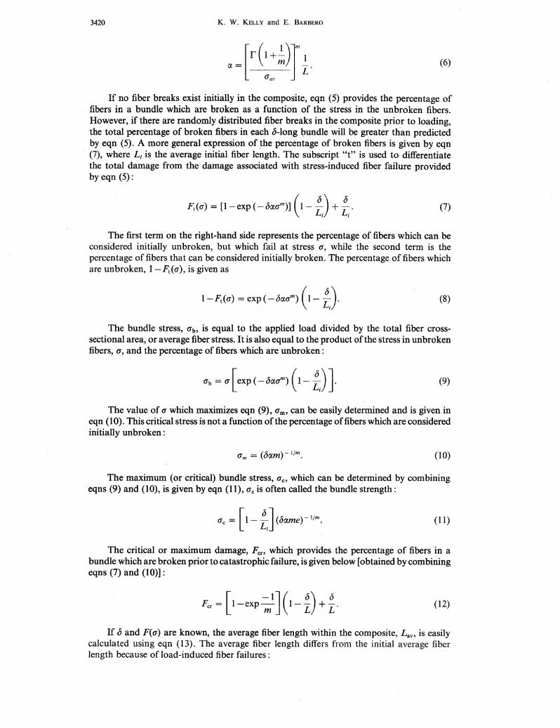
Rather than represent the composite. as a series of bundles ~ in length, the compositemay also be considered a colle~tion of cylinders, each containing a single broken fiber asshown in Fig. 3. A cylinder with a volume equal to the average volume of the cylindersshown in Fig. 3 can be considered a representative volume element (RVE). The total lengthoffiber contained in the RVE is equal to the average fiber length in the composite (neglectingend effects). Therefore, the volume of the RVE, VRVE , is simply the volume associated witha fiber of average length, Lav , divided by the fiber volume fraction:

(14)

where VRVE = volume of RVE,D = fiber diameter,VF = ~ber volume fraction.

As the matrix creeps, the following sequence occurs: the stress on the fibers increases,fibers break, the average fiber length within the composite decreases, and the size of theRVE decreases to reflect the increased amount of damage. As the RVE volume decreases,the longitudinal strain corresponding to a given applied load increases because the effectsof the broken fiber in the center become proportionately larger. Theoretically, the effect offiber breaks could be calculated numerically by determining the longitudinal strain inan RVE whose volume is continuously decreasing to account for accumulating damage.Forru'natelY-,oecausefieithet the bUIldle stress, O"b, nor the iheffecti"elength,b,arefll.Dctionsof the RVE volume, a method exists, which will be described, to calculate the compositestrain using simulation results from an RVE of constant volume. The RVE volume can bechosen arbitrarily, with the stipulation that it be long and tall enough' to prevent itsboundaries from significantly altering the stress field surrounding a fiber break. It will beshown that the evolution of the average fiber length (or RVE volume), as well as creepstrain can be easily calculated if the bundle stress, O"b, the ineffective length, ~, and the initialaverage fiber length are known. While the time-dependent value of O"b can be accuratelydetermined using analytic models, the time-dependent prediction of ~ often requires anumerical model.

Matrix surroundingbreak

Fig. 3. Model of composite as cylinders containing a fiber break.

3422 K. W. KELLY and E. BARBERO

NUMERICAL MODEL

A FEM using ANSYS (1991) has been developed to calculate the response of acomposite under longitudinal tension on a RVE containing one internal fiber break. Themodel calculates the values of b, the fiber bundle stress, (jb, and the average longitudinalstrain as functions of time.

The numerical analysis will present modeling results of a titanium matrix, alumina­fiber composite. The alumina fibers have 140 J1m diameters which are representative ofsingle crystal Saphikon fibers. The properties of both the matrix and the fiber used in themodel are listed in Appendix 1.

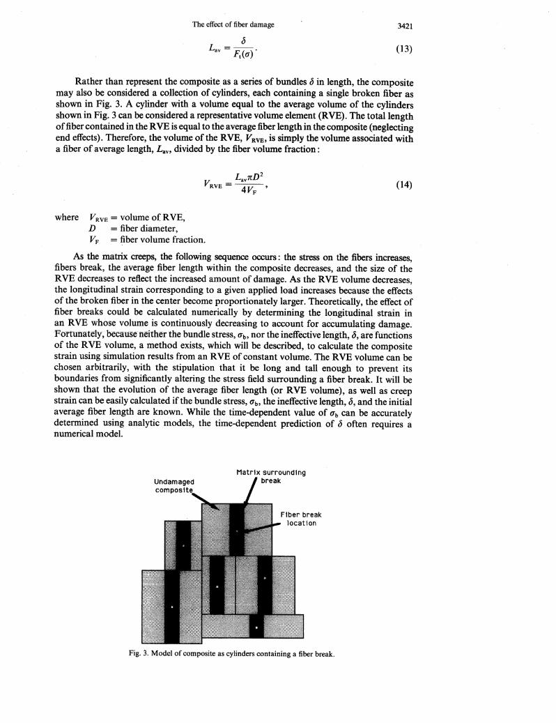
An axisymmetric view of the finite element model is shown in Fig. 4. This is the typicalconfiguration suggested by the cylindrical assemblage model (Hashin and Rosen, 1964;Christensen, 1979 ; Mikata and Taya, 1985 ; Hill, 1965). A ring ofmatrix lnaterial surroundsthe fiber. The thickness of the matrix ring corresponds to a composite with a 30% fibervolume. In this paper, only coulomb friction resists sliding at the fiber-matrix interface.Sliding occurs when shear at the interface exceeds the product of the compressive forceacross the interface and the coefficient of friction (Appendix 1). A ring of material withhomogenized .properties of the undamaged composite is coaxially located outside of andrigidly connected to the ring of matrix. The properties of the homogenized composite arethose of the undamaged material (no fiber breaks). The boundary conditions which areused in the model corresponding to Fig. 4 are described as follows:

. 1. The model is axisymmetric.2. The bottom surface of both the matrix and undamaged composite cylinders allows

zero axial displacement. When the fiber is considered unbroken, its bottom surface allowsno axial ~isplacement. When the fiber is considered broken, the bottom surface of the fiberis allowed to move in the positive z-direction, but not in the negative.

3. Thetop surfac_e of the model remains planar in response to longitudinal loads.4. There are no restraints to radial displacements except along the centerline of the

fiber.

HOMOGENIZED PROPERTIES OF UNDAMAGED COMPOSITE

The success of modeling the stress field surrounding a fiber break hinges on accuratelymodeling the behavior of the undamaged composite. The composite properties E., £2,CTE., CTE2, G2h V2h as well as creep response are needed to predict the response of the

>­'­4-'(J)

EE>­ene.­o(f)

X«

tForce

1111111111!11111111111111111!11111!1!11111111111111~11II

x

170ILm....... 1"-.. R

O ~,"" undamagedmatrix W" composite

Fig. 4. Model of the RVE.

The effect of fiber damage 3423

composite to thermal and mechanical loading. The homogenized composite properties (withthe exception of the creep response) were determined using micromechanics (Agarwal andBroutman, 1990; Everett, 1991 ; Taya, 1989).

CREEP RESPONSE OF UNDAMAGED COMPOSITE

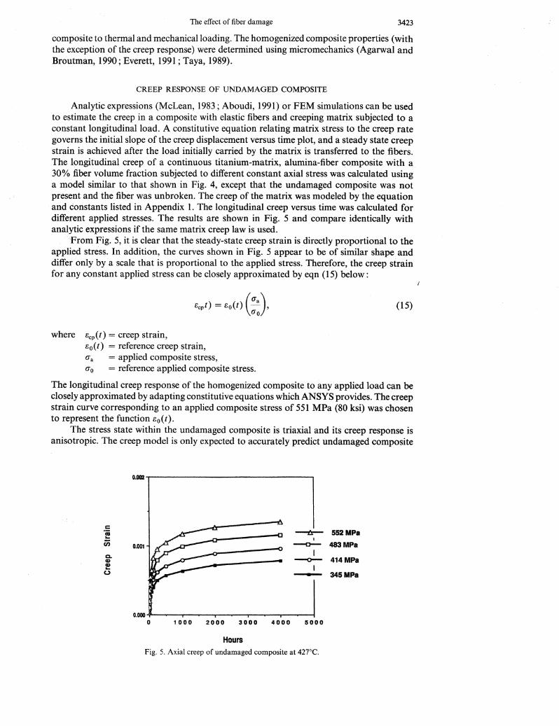
Analytic expressions (McLean, 1983; Aboudi, 1991) or FEM simulations can be usedto estimate the creep in a composite with elastic fibers and creeping matrix subjected to aconstant longitudinal load. A constitutive equation relating matrix stress to the creep rategoverns the initial slope of the creep displacement versus time plot, and a steady state creepstrain is achieved after the load initially carried by the matrix is transferred to the fibers.The longitudinal creep of a continuous titanium-matrix, alumina-fiber composite with a,30% fiber volume fraction subjected to different constant axial stress was calculated ~sing

a model similar to that shown in Fig. 4, except .that the undamaged composite was notpresentand the fiber was unbroken. The creep of the matrix was modeled by the equationand constants listed in Appendix 1. The longitudinal creep versus time was calculated fordifferent applied stresses. The results are shown in Fig. 5 and compare identically withanalytic expressions if the same matrix creep law is used.

"From Fig. 5, it is clear that the steady-state creep strain is directly prop~rtional to theapplied stress. In addition, the curves shown in Fig. 5 appear to be of similar shape anddiffer only by a scale that is proportional to the applied stress. Therefore, the creep strainfor any constant applied stress can be closely approximated by eqn (15) below:

(15)

where 8cp(t) = cre-ep strain,8o(t) = reference creep strain,(Ja = applied conlposite stress,(Jo = reference applied composite stress.

The longitudinal creep response of the homogeni~ed composite to any applied load can beclosely approximated by adapting constitutive equations which ANSYS provides. The creepstrain curve corresponding to an applied composite stress of 551 MPa (80 ksi) was chosento represent the function 8o(t).

The stress state within the undamaged composite is triaxial and its creep response isanisotropic. The creep model is only expected to accurately predict undamaged composite

0.002.....-------------------.

c'li ---t!-- 552MPaa- Ien 0.001 --0-- 483MPa

a.. ICD ---0-- 414MPaCD Ia-u ---.- 345MPa

0.000 ..;I-_-__---.~_-...___r_- - _____f

o 1000 2000 3000 4000 5000

HoursFig. 5. Axial creep of undamaged composite at 427°C.

3424 K. W. KELLY and E. BARBERO

creep strain when it is subjected to a pure axial stress. Furthermore, the function 8o(t)applies when the applied load is constant. If the stresses within a region of the undamagedcomposite vary significantly over the time during which load is applied, then the model maynot correctly predict the local creep rate. For example, if the stress within a region of theundamaged composite increases with time, the model may underpredict the local creep rate.Nevertheless, the authors believe that the model should represent reasonably well the creepresponse of the undamaged composite since axial stress dominates and the variation of thestress magnitude within the undamaged composite is relatively snlall.

NUMERICAL MODEL RESULTS

Numerical simulations of the model described in Fig. 4 were performed assumingcoefficient of friction values, jl, at the fiber-matrix interface of either 0.33 and 1.0. Thesetwo values of J1 are used to simulate, respectively, either a weak or strong interfacial shearstrength. In either case, cooldown from 927 to 427°C is simulated. Next, a 689.4 MPa (100ksi) stress is applied and held co'nstant for 4000 hours.

Following cooldown, a radial compressive stress of approximately 65 MPa existsinitially at the fiber-matrix interface as a result of residual stresses resulting from cooldown.This compressive stress, combined with the assumed coefficient of friction value, providesthe necessary shear stress which must be overcome for slip to occur at the fiber-matrixinterface. When a coefficient offriction of 1.0 is assumed, the initial interfacial shear strengthis 65 MPa. This value corresponds to a strong interface. Similarly, when the coefficientvalue is 0.33, the interface strength is proportionately lower (23.3 MPa). This value istypical of fairly weakly bonded interfaces. Over the 4000 hr period of load application, thecompressive stress at the interface decreases by about 500/0 (matrix relaxation)which causesthe interface strength, in either case, to decrease accordingly.

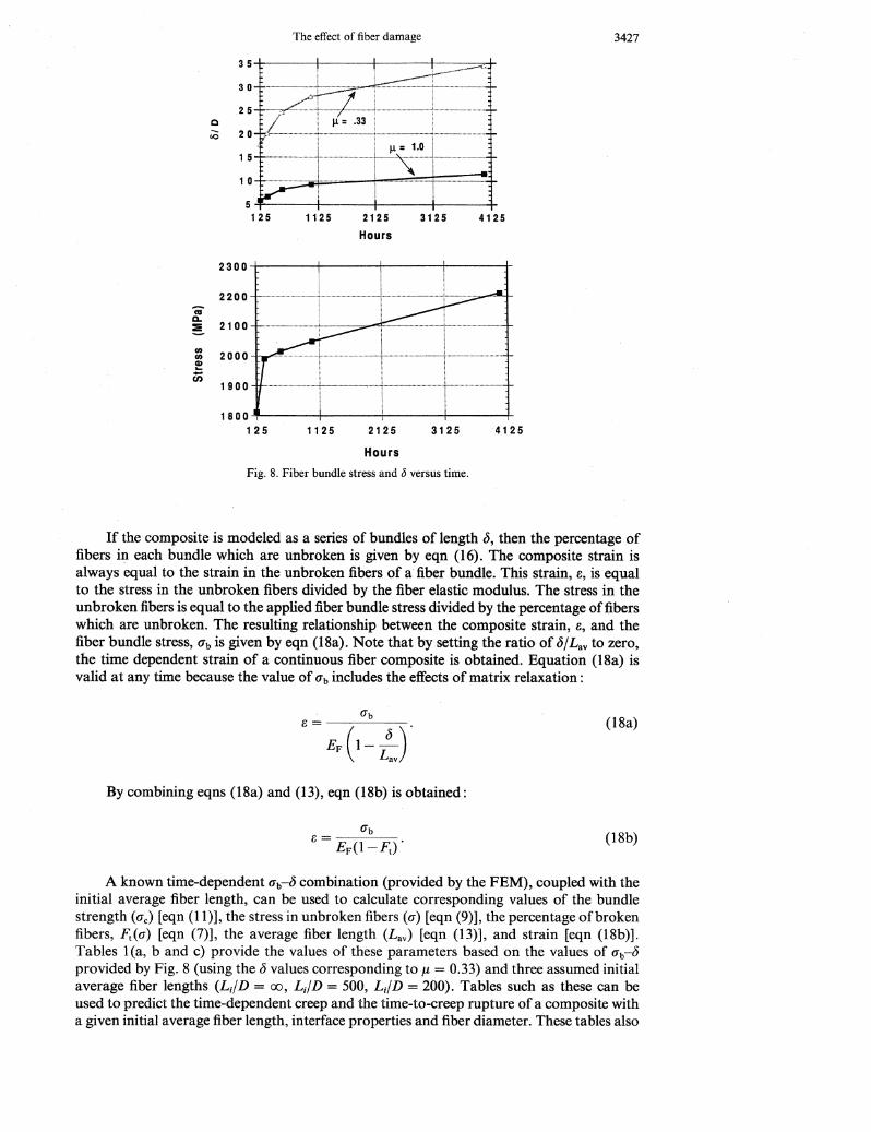
T-hebundle stress, Ub, provided by the axial stress in the fiber near the top of the model,is not a function of the value of the coefficient of friction. The bundle stress increases from1296 to 2213 MPa over the 4000 hr span.

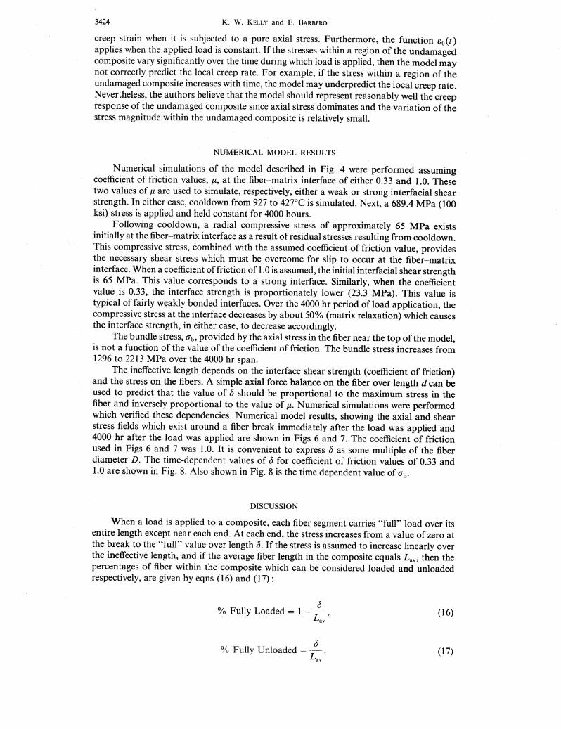
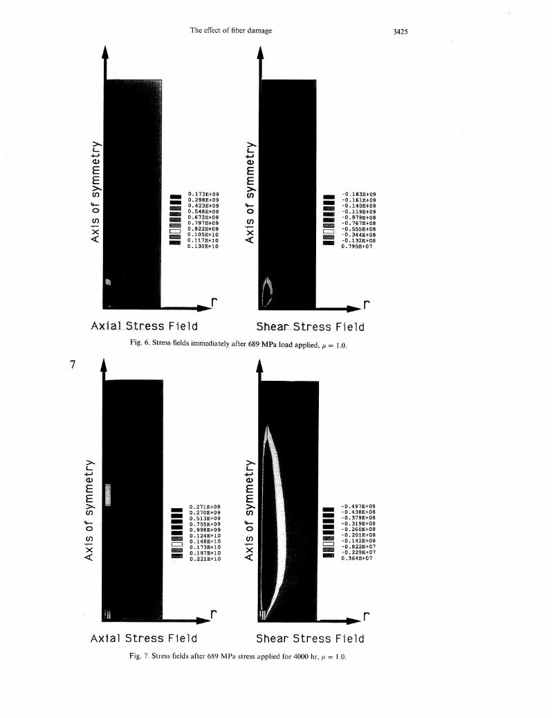
The ineffective length depends on the interface shear strength (coefficient of friction)and the stress on the fibers. A simple axial force balance on the fiber over length d can beused to predict that the value of () should be proportional to the maximum stress in thefiber and inversely proportional to the value of jl. Numerical simulations were performedwhich verified these dependencies. Numerical model results, showing the axial and shearstress fields which exist around a fiber break immediately after the load was applied and4000 'hr after the load was applied are shown in Figs 6 and 7. The coefficient of frictionused in Figs 6 and 7 was 1.0. It is convenient to express () as some multiple of the fiberdiameter D. The time-dependent values of () for coefficient of friction values of 0.33 and1.0 are shown in Fig. 8. Also shown in Fig. 8 is the time dependent value OfUb.

DISCUSSION

When a load is applied to a composite, each fiber segment carries "full" load over itsentire length except near each end. At each end, the stress increases from a value of zero atthe break to the "full" value over length (). If the stress is assumed to increase linearly overthe ineffective length, and if the average fiber length in the composite equals Lav , then thepercentages of fiber within the composite which can be considered loaded and unloadedrespectively, are given by eqns (16) and (17) :

()% Fully Loaded = 1- L

av

'

b% Fully Unloaded = L

av

•

(16)

(17)

The effect of fiber damage 3425

__~r____~:r

>..L

-i--'(l)

EE>-..

-O.183E+09-O.173E+09 en -O.298E+09 -O.161E+09<t- - O.423E+09 <t- - -O.140E+090 - O.548E+09 0 --O.119E+09

ifili ,..en -O.672E+09 --O.979E+08

O.797E+09 en -O.767E+08.- rmm O.922E+09 .- ~ -O.555E+08X c:::J O.105E+I0 X. c:::J -O.344E+08« ~ O.117E+I0 « ~ -O.132E+08.. O.130E+I0 -- O.795E+07

Fig. 6. Stress fields immediately after 689 MPa load applied, J1 = 1.0.

___~r__..~r

~ >..L L4-J -i--'(J) (l)

E EE E>.. O.271E+08 >-. - -O.497E+08(J) -O.270E+09 en -O.438E+08-O.513E+09 --O.379E+08<t- - O.755E+09 <t- - -O.319E+080 -O.998E+09 0 --O.260E+08- O.124E+I0 - -O.201E+08(J) IiIII O.148E+I0 en IllIIIII -O.142E+08.- c::J O.173E+I0 .- c:::J -O.822E+07X BliID O.197E+I0 X Ii:ilillB -O.229E+07« -O.221E+I0 « .. O.364E+07

7

Axial Stress Field Shear Stress Fi eld

Fig. 7. Stress fields after 689 MPa stress applied for 4000 hr, Ii = 1.0.

The effect of fiber damage 3427

412531252125

Hours

1125

3 5~----+----+------t---~

:: ;~~~ ~~~:'1 5 -.-....-...--l- ....----+.~~:~+-·---1 0 ·__·························· ..t················· ~

5125

Q

to

2300-l----~---~----+------t-

2 20 0 -+-.......................................•............................................+ ! ~~"--.-

= 2 0 0 0 -I-..~ ~ ; ~ ;-

~(j)

asa.~ 2100

1 9 0 0 -H- ~ ····,····..···i······ ·····················..·········..+ ;-

'412531251125 2125

Hours

Fig. 8. Fiber bundle stress and {) versus time.

1 800 ..J!I!II~----+----i------+-----t­

125

If the composite is modeled as a series of bundles of length b, then the percentage offibers ill' each bundle which are unbroken is given by eqn (16). The composite strain isalways equal to the strain in the unbroken fibers of a' fiber bundle. This strain, 8, is equalto the stress in the unbroken fibers divided by the fiber elastic modulus. The stress in theunbroken fibers is equal to the applied fiber bundle stress divided by the percentage offiberswhich are unbroken. The resulting relationship between the composite strain, 8, and thefiber bundle stress, O'b is given by eqn (I8a). Note that by setting the ratio of b/Lav to zero,the time dependent strain of a continuous fiber composite is obtained. Equation (I8a) isvalid at any time because the value of O"b includes the effects of matrix relaxation:

(18a)

By combining eqns (I8a) and (13), eqn (I8b) is obtained:

(18b)

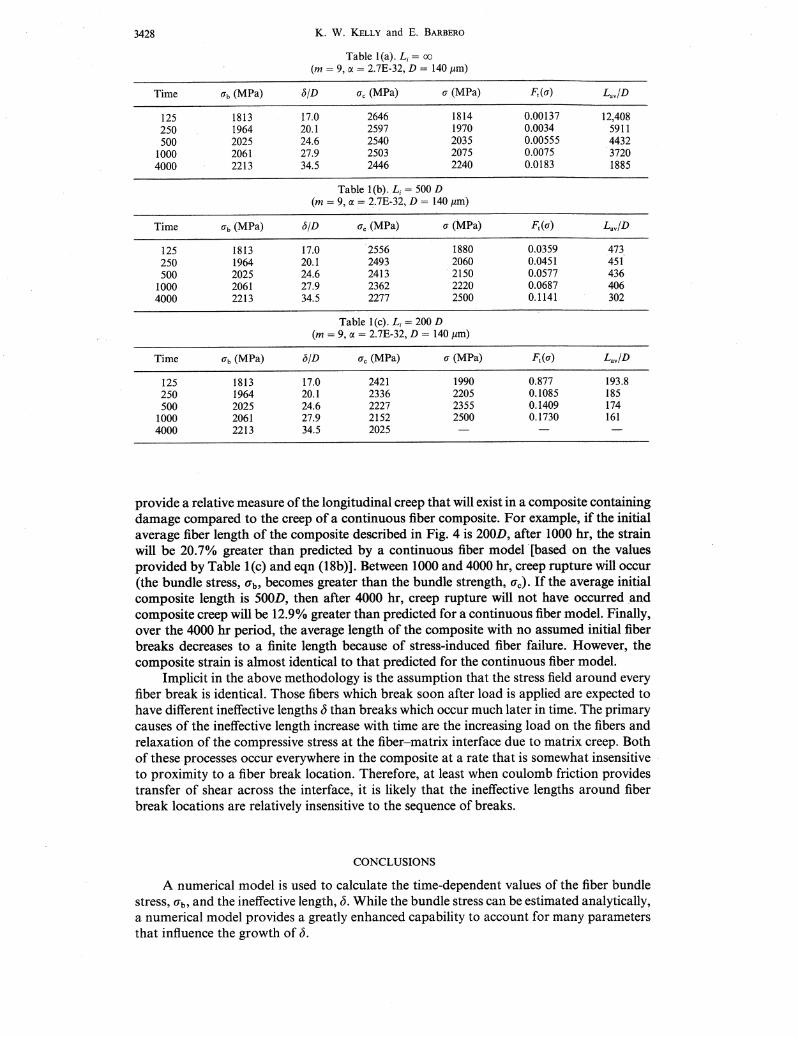
A known time-dependent O"b-b combination (provided by the FEM), coupled with theinitial average fiber length, can be used to calculate corresponding values of the bundlestrength (ae) [eqn (11)], the stress in unbroken fibers (a) [eqn (9)], the percentage of brokenfibers, Ft(a) [eqn (7)], the average fiber length (Lav ) [eqn (13)], and strain [eqn (18b)].Tables 1(a, b and c) provide the values of these parameters based on the values of Ub-t5

provided by Fig. 8 (using the b values corresponding to J1 = 0.33) and three assumed initialaverage fiber lengths (L;/D = 00, L;/D = 500, L;/D = 200). Tables such as these can beused to predict the time-dependent creep and the time-to-creep rupture of a composite witha given initial average fiber length, interface properties and fiber diameter. These tables also

3428 K. W. KELLY and E. BARBERO

Table 1(a). L j = CIJ

(m = 9, (X = 2.7E-32, D = 140 /lm)

Time O"b (MPa) bjD (Jc (MPa) (J (MPa) Ft«(J) LavjD

125 1813 17.0 2646 1814 0.00137 12,408250 1964 20.1 2597 1970 0.0034 5911500 2025 24.6 2540 2035 0.00555 4432

1000 2061 27.9 2503 2075 0.0075 37204000 2213 34.5 2446 2240 0.0183 1885

Table l(b). L j = 500 D(m = 9, (X = 2.7E-32, D = 140/lm)

Time (Jb (MPa) bjD (Jc (MPa) (J (MPa) Ft«(J) LavjD

125 1813 17.0 2556 1880 0.0359 473250 1964 20.1 2493 2060 0.0451 451500 2025 24.6 2413 2150 0.0577 436

1000 2061 27.9 2362 2220 0.0687 4064000 2213 34.5 2277 2500 0.1141 302

Table l(c). L j = 200 D(m = 9, (X = 2.7E-32, D = 140/lm)

Time (Jb (MPa) bjD (Jc (MPa) (J (MPa) Ft«(J) LavjD

125 1813 17.0 2421 1990 0.877 193.8250 1964 20.1 2336 2205 0.1085 185500 2025 24.6 2227 2355 0.1409 174

1000 2061 27.9 2152 2500 0.1730 1614000 2213 34.5 2025

provide a relative measure of the longitudinal creep that will exist in a composite containingdamage compared to the creep of a continuous fiber composite. For example, if the initialaverage fiber length of the composite described in Fig. 4 is 200D, after 1000 hr, the strainwill be 20.70/0 great~r than predicted by a continuous fiber model '[based on the valuesprovided by Table 1(c) and eqn (18b)]. Between 1000 and 4000 hr, creep rupture will occur(the bundle stress, O'b, becomes greater than the bundle strength, uc)' If the average initialcomposite length is 500D, then after 4000 hr, creep rupture will not have occurred ,andcomposite creep will be 12.9% greater than predicted for a continuous fiber model. Finally,over the 4000 hr period, the average length of the composite with no assumed initial fiberbreaks decreases to a finite length because of stress-induced fiber failure. However, thecomposite strain is almost identical to that predicted for the continuous fiber model.

Implicit in the above methodology is the assumption that the stress field around everyfiber break is identical. Those fibers which break soon after load is applied are expected tohave different ineffective lengths b than breaks which occur much later in time. The primarycauses of the ineffective length increase with time are the increasing load on the fibers andrelaxation of the compressive stress at the fiber-matrix interface due to matrix creep. Bothof these processes occur everywhere in the composite at a rate that is somewhat insensitiveto proximity to a fiber break location. Therefore, at least when coulomb friction providestransfer of shear across the interface, it is likely that the ineffective lengths around fiberbreak locations are relatively insensitive to the sequence of breaks.

CONCLUSIONS

A numerical model is used to calculate the time-dependent values of the fiber bundlestress, O'b, and the ineffective length, lJ. While the bundle stress can be estimated analytically,a numerical model provides a greatly enhanced capability to account for many parametersthat influence the growth of b.

The effect of fiber damage 3429

A set of equations is introduced which can be used to calculate the time-dependentstrain, time to rupture, .and the time-dependent strength of a composite, given the time­dependent O"b-l5 combination. In addition, the accuracy of the simple continuous fiber modelcreep prediction can be easily determined. Finally, the ability to determine the relativeimportance of many parameters on strength and creep response is provided.

Acknowledgelnents-Provision of the ANSYS finite element program and technical support by Swanson AnalysisSystems of Washington, PA was greatly appreciated. The research was sponsored by DARPA and 3M contractMDA972-90-C-018.

REFERENCES

Aboudi, J. (1991). Mechanics ofComposite Materials. Elsevier, NY.Agarwal, B. D. and Broutman, C. J. (1990). Analysis and Performance ofFiber Composites. John Wiley, NY.ANSYS (1991). Theoretical Manual, Revision 4.4. Swanson Analysis Systems Inc., Houston, PA.Christensen, R. and Lo, K. (1979). Solutions for effective shear properties in three phase sphere and cylinder

models. J. Mech. Phys. Solids 27,315-330.Deve, H. (1992). Personal communication. 3M Corporation, St Paul, MN.Everett, R. K. and Arsenault, R. J. (1991). Metal Matrix Composites: Mechanisms and Properties. Academic

Press, Boston.Hashin, Z. and Rosen, B. W. (1964). The elastic moduli of fiber-reinforced materials. J. Appl. Mech. 31,232.Hill~ R. (1965). Theory of mechanical properties of fiber-strengthened materials: III. Self-consistent model. J.

Mech. Phys. Solids 13, 198.Kelly, A. and Street, K. (1972). Creep of discontinuous fiber composites. Proc. Roy. Soc. Lond. A328, 283-293.Lifshitz, J. and Rotem, A. (1970). Time-dependent longitudinal strength of unidirectional fibrous composites.

Fiber Sci. Technol.3, 1-21.McLean, M. (1983). Directionally Solidified Materialsfor High Temperature Service. The Metal Society, London.Metals Handbook (1961). (8th Edn, Vol. 1). American Society for Metals, Novelty, OH.Mikata, Y. and Taya, M. (1985). Stress field in a coated continuous fiber composite subjected to thermo­

mechanical loadings. J. Compos. Mater. 19,554-578.Nimmer, R. P., Bankert, R. J., Russell, E. S. and Smith, G. A. (1989). Micromechanical modeling of fiber/matrix

interface effects in SiC/Ti metal matrix composites. Proc. 1989 ASM Materials Week, Indianapolis, IN,7Q~QQ~r 1989.

Rosen, B. W. (1964). The tensile failure of fibrous composites. AIAA J12(1 1), 1985-1991.Steif, P. (1984). Stiffness reduction due to fiber breakage. J. Compos. Mater. 17, 153-172.Taya, M. and Arsenault, R: (1989). Metal Matrix Composites. Pergamon Press, Oxford.Weibull, W. (1951). A statistical distribution function of wide applicability. J. Appl. Mech. 18,293-296.Wright, P. K., Russell, E., Nimmer R. and Smith, G. (1989). Creep in Ti/SiC composites. Presented at TVIS

Annual Meeting, Las Vegas, Nevada, 27 February-2 March 1989.

APPENDIX I

Properties of Ti 6-4 at 427°CElastic Modulust 87.5 GPa,Pois~on Ratiot 0.3,CTE§ 10.44 E-6°C- 1

,

Shear Modulust GPa,Yield Strengtht 496 MPa,Creep equation II de/dt = A(e-B/T)(t-C)(aD).

A = 4.063 hr-o.366 MPa -1.715,

B = 30,000 K,C = -0.634,D = 1.715,T = 700 K,t = time (hr),a = stress (MPa).

Properties ofinterfaceCoefficient of friction 0.33 or 1.0.

Properties ofalumina fibers at 427°CElastic Modulustt 379 GPa,Poisson Ratiott 0.27,CTEtt 8.28 E-6°C- 1

,

Shear Modulus 148.9 GPa,Average Strengthtt 2758 MPa,§§Weibull Modulustt 9.

t Nimmer et .al. (1989), Metals Handbook (1959).t Nimmer (1989).§Metals Handbook (1961).II Wright et al. (1989).tt Deve (1992).tt Taya (1989).§§ Strength based on 2.54 cm gauge length.