THE EFFECT OF METAL FOIL TAPE DEGRADATION ON THE LONG-TERM RELIABILITY OF PV MODULES

N. Robert Sorensen, Michael A. Quintana, Joseph D. Puskar and Samuel J. Lucero

Sandia National Laboratories1, P.O. Box 5800, Albuquerque, New Mexico 87185

ABSTRACT

A program is underway at Sandia National Laboratories1 to predict long-term reliability of photovoltaic systems. The vehicle for the reliability predictions is a Reliability Block Diagram (RBD), which models system behavior. Because this model is based mainly on field failure and repair times, it cannot currently be used to accurately predict end-of-life. In order to be truly predictive, physics-informed degradation processes and failure mechanisms need to be included in the model. This paper describes accelerated life testing of metal foil tapes used in thin-film PV modules, and how tape joint degradation, a possible failure mode, can be incorporated into the model.

BACKGROUND A vibrant photovoltaic industry has emerged in recent years primarily as a result of exponential market growth, dynamic changes in technologies, and innovative approaches to what the ideal business model(s) will be in the future. Throughout the recent turbulence, reliability of photovoltaic systems has continued to be a dominant concern of the supply chain, from materials manufacturers to component manufacturers to system integrators, and finally the end customer. Increasingly savvy customers are asking for increasingly sophisticated and complex information as due diligence is performed prior to investing massive amounts of capital. Indeed, photovoltaics is industry no longer a cottage industry, but as maturation occurs so do growth pains and challenges. One such challenge is to develop predictive capabilities to evaluate potential failure modes and the probability of failure in photovoltaics and apply this knowledge to predict service life. One such tool that assists in answering the challenge is accelerated life tests (ALT’s). A key motivation for developing a comprehensive set of ALT’s is the ability to translate the information acquired into cost effectiveness of components and systems. Additionally, carefully developed ALT’s assist in development of high product integrity and short time-to-market development cycles. ALT’s, however, are not standardized in the photovoltaics arena. It is important to remember that qualification tests,

1 Sandia is a multiprogram laboratory operated by Sandia Corporation, a Lockheed Martin Company, for the United States Department of Energy’s National Nuclear Security Administration under contract DE-AC04-94AL85000

the most common type of accelerated tests recognized, do not provide a probability of failure; ideally the qualification test is meant to be passed. ALT’s are destructive tests meant to uncover expected failures and provide an understanding of the physics of failure; and furthermore to develop a statistical base from which to make predictions. The study described in this paper is the beginning of an application of accelerated life testing of a single packaging element used in some photovoltaic designs with an expectation of a much more rigorous application of ALT’s in the future. [1] Packaging of a thin film PV technology was selected to demonstrate how materials degradation phenomena can be included in the RBD. One high likelihood failure process identified through a Failure Modes and Effects Analysis (FMEA) of the thin-film technology was degradation of the metal foil tape joints. To generate degradation data, accelerated tests were run on samples with overlapping tape joints. The degradation data obtained in these experiments are being used in the RBD model.

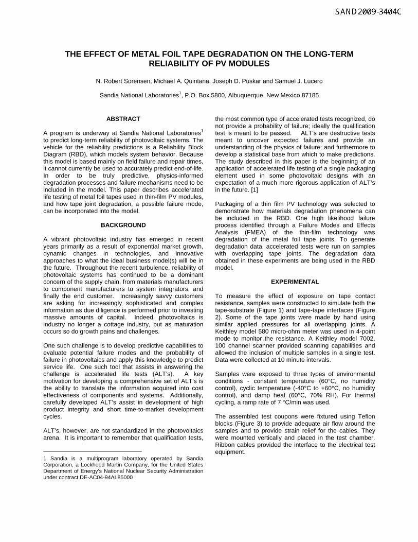
EXPERIMENTAL To measure the effect of exposure on tape contact resistance, samples were constructed to simulate both the tape-substrate (Figure 1) and tape-tape interfaces (Figure 2). Some of the tape joints were made by hand using similar applied pressures for all overlapping joints. A Keithley model 580 micro-ohm meter was used in 4-point mode to monitor the resistance. A Keithley model 7002, 100 channel scanner provided scanning capabilities and allowed the inclusion of multiple samples in a single test. Data were collected at 10 minute intervals. Samples were exposed to three types of environmental conditions - constant temperature (60°C, no humidity control), cyclic temperature (-40°C to +60°C, no humidity control), and damp heat (60°C, 70% RH). For thermal cycling, a ramp rate of 7 °C/min was used. The assembled test coupons were fixtured using Teflon blocks (Figure 3) to provide adequate air flow around the samples and to provide strain relief for the cables. They were mounted vertically and placed in the test chamber. Ribbon cables provided the interface to the electrical test equipment.

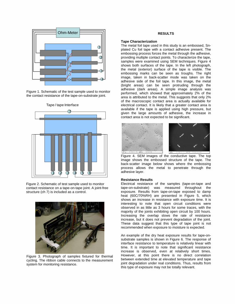
Figure 1. Schematic of the test sample used to monitor the contact resistance of the tape-on-substrate joint.

Figure 2. Schematic of test sample used to monitor contact resistance on a tape-on-tape joint. A joint-free structure (ch 7) is included as a control.

Figure 3. Photograph of samples fixtured for thermal cycling. The ribbon cable connects to the measurement system for monitoring resistance.

RESULTS

Tape Characterization The metal foil tape used in this study is an embossed, Sn-plated Cu foil tape with a contact adhesive present. The embossing process forces the metal through the adhesive, providing multiple contact points. To characterize the tape, samples were examined using SEM techniques. Figure 4 shows both surfaces of the tape. In the left photograph, the metal (exterior) surface of the tape is visible. The embossing marks can be seen as troughs. The right image, taken in back-scatter mode was taken on the adhesive side of the foil tape. In this image, the metal (bright areas) can be seen protruding through the adhesive (dark areas). A simple image analysis was performed, which showed that approximately 2% of the area is attributed to the metal. This suggests that only 2% of the macroscopic contact area is actually available for electrical contact. It is likely that a greater contact area is available if the tape is applied using high pressure, but given the large amounts of adhesive, the increase in contact area is not expected to be significant.

Figure 4. SEM images of the conductive tape. The top image shows the embossed structure of the tape. The back-scatter image below shows where the embossing process allows the metal to penetrate through the adhesive layer. Resistance Results Electrical resistance of the samples (tape-on-tape and tape-on-substrate) was measured throughout the exposure. Results from tape-on-tape exposed to damp heat (60C/70%RH) are presented in Figure 5, which shows an increase in resistance with exposure time. It is interesting to note that open circuit conditions were observed in as little as 3 hours for some traces, with the majority of the joints exhibiting open circuit by 100 hours. Increasing the overlap slows the rate of resistance increase, but it does not prevent degradation of the joint. These data suggest that this type of tape joint is not recommended when exposure to moisture is expected. An example of the dry heat exposure results for tape-on-substrate samples is shown in Figure 6. The response of interface resistance to temperature is relatively linear with time. It is important to note that significant resistance increase is observed, even at relatively short times. However, at this point there is no direct correlation between extended time at elevated temperature and tape joint degradation under real conditions. Thus, results from this type of exposure may not be totally relevant.

Ohm-Meter

1

2

3

4

5

6

7

8

9

10

1 2 3 4 5 6

7

Tape / tape Interface

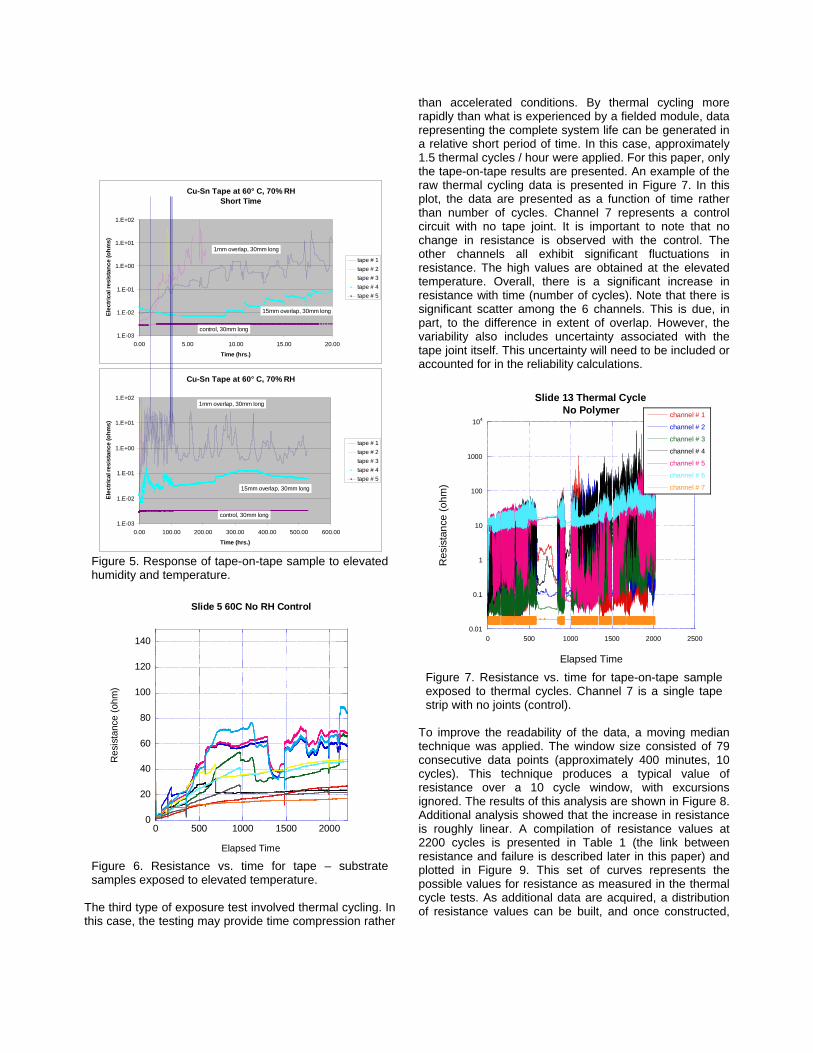
Figure 5. Response of tape-on-tape sample to elevated humidity and temperature.

Figure 6. Resistance vs. time for tape – substrate samples exposed to elevated temperature.

The third type of exposure test involved thermal cycling. In this case, the testing may provide time compression rather

than accelerated conditions. By thermal cycling more rapidly than what is experienced by a fielded module, data representing the complete system life can be generated in a relative short period of time. In this case, approximately 1.5 thermal cycles / hour were applied. For this paper, only the tape-on-tape results are presented. An example of the raw thermal cycling data is presented in Figure 7. In this plot, the data are presented as a function of time rather than number of cycles. Channel 7 represents a control circuit with no tape joint. It is important to note that no change in resistance is observed with the control. The other channels all exhibit significant fluctuations in resistance. The high values are obtained at the elevated temperature. Overall, there is a significant increase in resistance with time (number of cycles). Note that there is significant scatter among the 6 channels. This is due, in part, to the difference in extent of overlap. However, the variability also includes uncertainty associated with the tape joint itself. This uncertainty will need to be included or accounted for in the reliability calculations.

Figure 7. Resistance vs. time for tape-on-tape sample exposed to thermal cycles. Channel 7 is a single tape strip with no joints (control).

To improve the readability of the data, a moving median technique was applied. The window size consisted of 79 consecutive data points (approximately 400 minutes, 10 cycles). This technique produces a typical value of resistance over a 10 cycle window, with excursions ignored. The results of this analysis are shown in Figure 8. Additional analysis showed that the increase in resistance is roughly linear. A compilation of resistance values at 2200 cycles is presented in Table 1 (the link between resistance and failure is described later in this paper) and plotted in Figure 9. This set of curves represents the possible values for resistance as measured in the thermal cycle tests. As additional data are acquired, a distribution of resistance values can be built, and once constructed,

Cu-Sn Tape at 60° C, 70% RHShort Time

1.E-03

1.E-02

1.E-01

1.E+00

1.E+01

1.E+02

0.00 5.00 10.00 15.00 20.00

Time (hrs.)

Ele

ctr

ical

re

sis

tan

ce

(o

hm

s)

tape # 1

tape # 2

tape # 3

tape # 4

tape # 5

15mm overlap, 30mm long

1mm overlap, 30mm long

control, 30mm long

Cu-Sn Tape at 60° C, 70% RH

1.E-03

1.E-02

1.E-01

1.E+00

1.E+01

1.E+02

0.00 100.00 200.00 300.00 400.00 500.00 600.00

Time (hrs.)

Ele

ctr

ica

l re

sis

tan

ce

(o

hm

s)

tape # 1

tape # 2

tape # 3

tape # 4

tape # 5

15mm overlap, 30mm long

1mm overlap, 30mm long

control, 30mm long

0

20

40

60

80

100

120

140

0 500 1000 1500 2000

Slide 5 60C No RH Control

Res

ista

nce

(ohm

)

Elapsed Time

0.01

0.1

1

10

100

1000

104

0 500 1000 1500 2000 2500

Slide 13 Thermal CycleNo Polymer channel # 1

channel # 2

channel # 3

channel # 4

channel # 5

channel # 6

channel # 7

Res

ista

nce

(o

hm

)

Elapsed Time

can be used to assign joint resistance values (at the module level) for a specific tape joint based on probability.

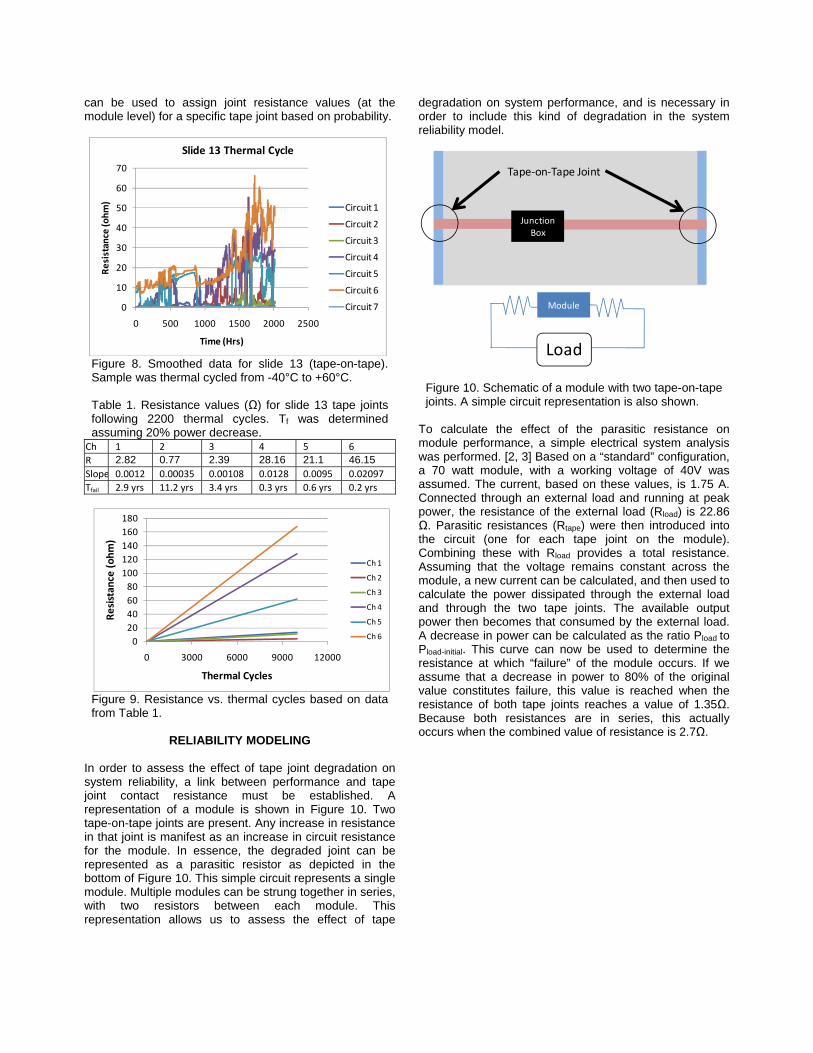
Figure 8. Smoothed data for slide 13 (tape-on-tape). Sample was thermal cycled from -40°C to +60°C.

Table 1. Resistance values (Ω) for slide 13 tape joints following 2200 thermal cycles. Tf was determined assuming 20% power decrease.

Ch 1 2 3 4 5 6

R 2.82 0.77 2.39 28.16 21.1 46.15 Slope 0.0012 0.00035 0.00108 0.0128 0.0095 0.02097

Tfail 2.9 yrs 11.2 yrs 3.4 yrs 0.3 yrs 0.6 yrs 0.2 yrs

Figure 9. Resistance vs. thermal cycles based on data from Table 1.

RELIABILITY MODELING

In order to assess the effect of tape joint degradation on system reliability, a link between performance and tape joint contact resistance must be established. A representation of a module is shown in Figure 10. Two tape-on-tape joints are present. Any increase in resistance in that joint is manifest as an increase in circuit resistance for the module. In essence, the degraded joint can be represented as a parasitic resistor as depicted in the bottom of Figure 10. This simple circuit represents a single module. Multiple modules can be strung together in series, with two resistors between each module. This representation allows us to assess the effect of tape

degradation on system performance, and is necessary in order to include this kind of degradation in the system reliability model.

Figure 10. Schematic of a module with two tape-on-tape joints. A simple circuit representation is also shown.

To calculate the effect of the parasitic resistance on module performance, a simple electrical system analysis was performed. [2, 3] Based on a “standard” configuration, a 70 watt module, with a working voltage of 40V was assumed. The current, based on these values, is 1.75 A. Connected through an external load and running at peak power, the resistance of the external load (Rload) is 22.86 Ω. Parasitic resistances (Rtape) were then introduced into the circuit (one for each tape joint on the module). Combining these with Rload provides a total resistance. Assuming that the voltage remains constant across the module, a new current can be calculated, and then used to calculate the power dissipated through the external load and through the two tape joints. The available output power then becomes that consumed by the external load. A decrease in power can be calculated as the ratio Pload to Pload-initial. This curve can now be used to determine the resistance at which “failure” of the module occurs. If we assume that a decrease in power to 80% of the original value constitutes failure, this value is reached when the resistance of both tape joints reaches a value of 1.35Ω. Because both resistances are in series, this actually occurs when the combined value of resistance is 2.7Ω.

0

10

20

30

40

50

60

70

0 500 1000 1500 2000 2500

Resistance (ohm)

Time (Hrs)

Slide 13 Thermal Cycle

Circuit 1

Circuit 2

Circuit 3

Circuit 4

Circuit 5

Circuit 6

Circuit 7

0

20

40

60

80

100

120

140

160

180

0 3000 6000 9000 12000

Resistance (ohm)

Thermal Cycles

Ch 1

Ch 2

Ch 3

Ch 4

Ch 5

Ch 6

Junction Box

Tape‐on‐Tape Joint

Module

Load

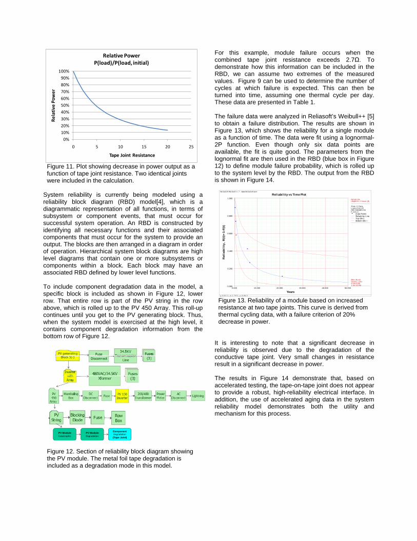
Figure 11. Plot showing decrease in power output as a function of tape joint resistance. Two identical joints were included in the calculation.

System reliability is currently being modeled using a reliability block diagram (RBD) model[4], which is a diagrammatic representation of all functions, in terms of subsystem or component events, that must occur for successful system operation. An RBD is constructed by identifying all necessary functions and their associated components that must occur for the system to provide an output. The blocks are then arranged in a diagram in order of operation. Hierarchical system block diagrams are high level diagrams that contain one or more subsystems or components within a block. Each block may have an associated RBD defined by lower level functions. To include component degradation data in the model, a specific block is included as shown in Figure 12, lower row. That entire row is part of the PV string in the row above, which is rolled up to the PV 450 Array. This roll-up continues until you get to the PV generating block. Thus, when the system model is exercised at the high level, it contains component degradation information from the bottom row of Figure 12.

Figure 12. Section of reliability block diagram showing the PV module. The metal foil tape degradation is included as a degradation mode in this model.

For this example, module failure occurs when the combined tape joint resistance exceeds 2.7Ω. To demonstrate how this information can be included in the RBD, we can assume two extremes of the measured values. Figure 9 can be used to determine the number of cycles at which failure is expected. This can then be turned into time, assuming one thermal cycle per day. These data are presented in Table 1. The failure data were analyzed in Reliasoft’s Weibull++ [5] to obtain a failure distribution. The results are shown in Figure 13, which shows the reliability for a single module as a function of time. The data were fit using a lognormal-2P function. Even though only six data points are available, the fit is quite good. The parameters from the lognormal fit are then used in the RBD (blue box in Figure 12) to define module failure probability, which is rolled up to the system level by the RBD. The output from the RBD is shown in Figure 14.

Figure 13. Reliability of a module based on increased resistance at two tape joints. This curve is derived from thermal cycling data, with a failure criterion of 20% decrease in power.

It is interesting to note that a significant decrease in reliability is observed due to the degradation of the conductive tape joint. Very small changes in resistance result in a significant decrease in power. The results in Figure 14 demonstrate that, based on accelerated testing, the tape-on-tape joint does not appear to provide a robust, high-reliability electrical interface. In addition, the use of accelerated aging data in the system reliability model demonstrates both the utility and mechanism for this process.

0%

10%

20%

30%

40%

50%

60%

70%

80%

90%

100%

0 5 10 15 20 25

Relative

Power

Tape Joint Resistance

Relative PowerP(load)/P(load, initial)

PV ModuleCatastrophic

PV ModuleDegradation

ComponentDegradation

(Tape Joint)

Re l iaSoft We ibul l++ 7 - www.Re l iaSoft.com

Reliability vs Time Plot

Years

Rel

iabi

lity

, R

(t)=

1-F(

t)

0.000 50.00010.000 20.000 30.000 40.0000.000

1.000

0.200

0.400

0.600

0.800

Re l iab i l i tyCB@90% 2-Sided [R]

Sl ide 13 Da taL ognorma l-2PRRX SRM MED FMF=6/S=0

D ata PointsReliability LineTop CB-I IBottom CB-I I

Mik e MundtSandia La bs5/26/20091:45:18 PM

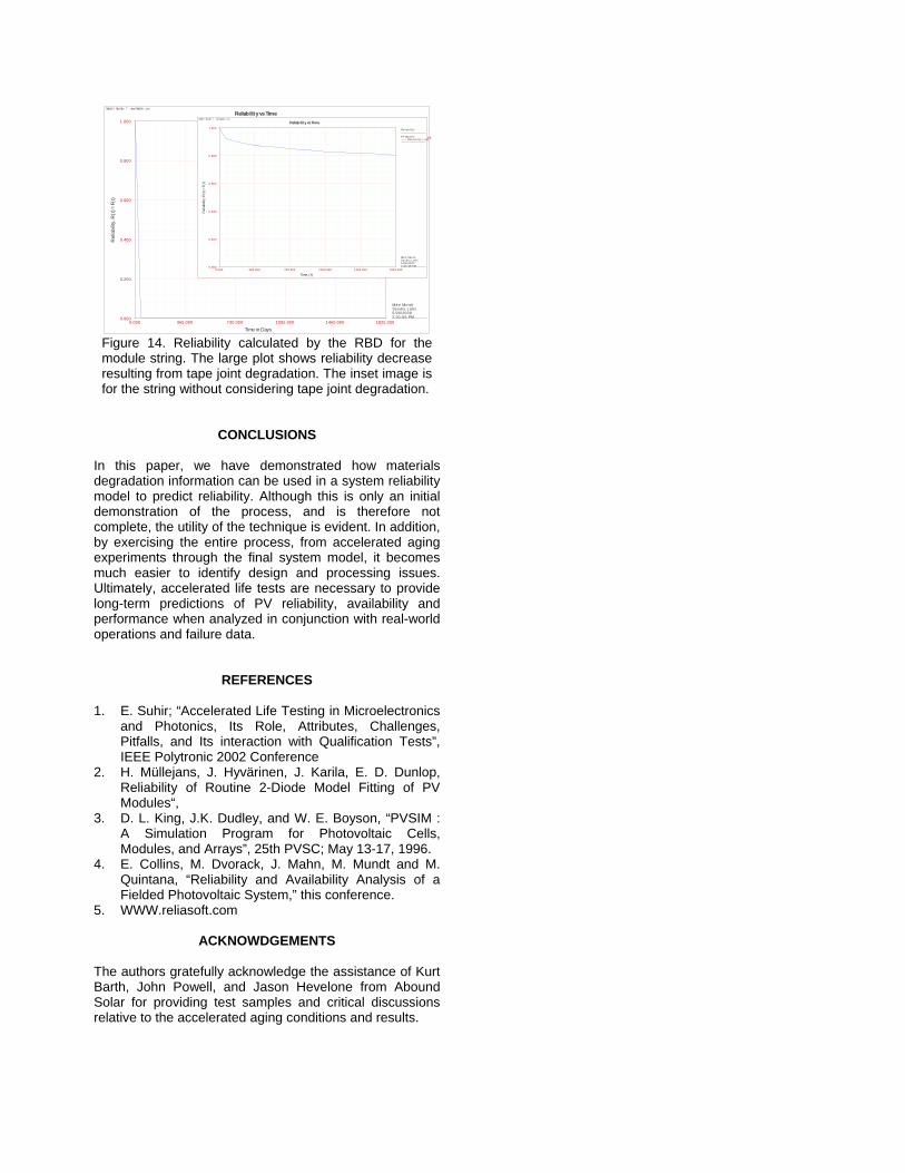
Figure 14. Reliability calculated by the RBD for the module string. The large plot shows reliability decrease resulting from tape joint degradation. The inset image is for the string without considering tape joint degradation.

CONCLUSIONS

In this paper, we have demonstrated how materials degradation information can be used in a system reliability model to predict reliability. Although this is only an initial demonstration of the process, and is therefore not complete, the utility of the technique is evident. In addition, by exercising the entire process, from accelerated aging experiments through the final system model, it becomes much easier to identify design and processing issues. Ultimately, accelerated life tests are necessary to provide long-term predictions of PV reliability, availability and performance when analyzed in conjunction with real-world operations and failure data.

REFERENCES 1. E. Suhir; “Accelerated Life Testing in Microelectronics

and Photonics, Its Role, Attributes, Challenges, Pitfalls, and Its interaction with Qualification Tests”, IEEE Polytronic 2002 Conference

2. H. Müllejans, J. Hyvärinen, J. Karila, E. D. Dunlop, Reliability of Routine 2-Diode Model Fitting of PV Modules“,

3. D. L. King, J.K. Dudley, and W. E. Boyson, “PVSIM : A Simulation Program for Photovoltaic Cells, Modules, and Arrays”, 25th PVSC; May 13-17, 1996.

4. E. Collins, M. Dvorack, J. Mahn, M. Mundt and M. Quintana, “Reliability and Availability Analysis of a Fielded Photovoltaic System,” this conference.

5. WWW.reliasoft.com

ACKNOWDGEMENTS The authors gratefully acknowledge the assistance of Kurt Barth, John Powell, and Jason Hevelone from Abound Solar for providing test samples and critical discussions relative to the accelerated aging conditions and results.

ReliaSoft BlockSim 7 - www.ReliaSoft.com

Reliability vs Time

Time in Days

Rel

iabi

lity,

R(t

)=F(

t)

0.000 1825.000365.000 730.000 1095.000 1460.0000.000

1.000

0.200

0.400

0.600

0.800

Re l iab i l i ty

PV ModuleRe l iab i l i ty L ine

Mik e MundtSandia L abs5/26/20092:31:05 PM

ReliaSoft BlockSim 7 - www.ReliaSoft.com

Reliability vs Time

Time, (t)

Rel

iabi

lity,

R(t

)=F(

t)

0.000 1825.000365.000 730.000 1095.000 1460.0000.900

1.000

0.920

0.940

0.960

0.980

Rel ia bi l ity

PV ModuleRe l ia bi l ity L ine

Mike MundtSand ia Labs5/26/20092:35:48 PM