Embed Size (px)
Citation preview
The Effect of Price Risk on Mongolian Copper Exports
by
Jiaxuan Gao
A thesis submitted to the Graduate Faculty of
Auburn University
in partial fulfillment of the
requirements for the Degree of
Master of Science
Auburn, Alabama
August 5, 2017
Keywords: Mongolia, Copper Ore, Price Risk, Demand Theory,
Differential Import Allocation Model
Copyright 2017 by Jiaxuan Gao
Approved by
Henry Kinnucan, Chair, Alumni Professor of Agricultural Economics and Rural Sociology
Patricia A. Duffy, Professor of Agricultural Economics and Rural Sociology
Yaoqi Zhang, Professor of School of Forestry and Wildlife Sciences
ii
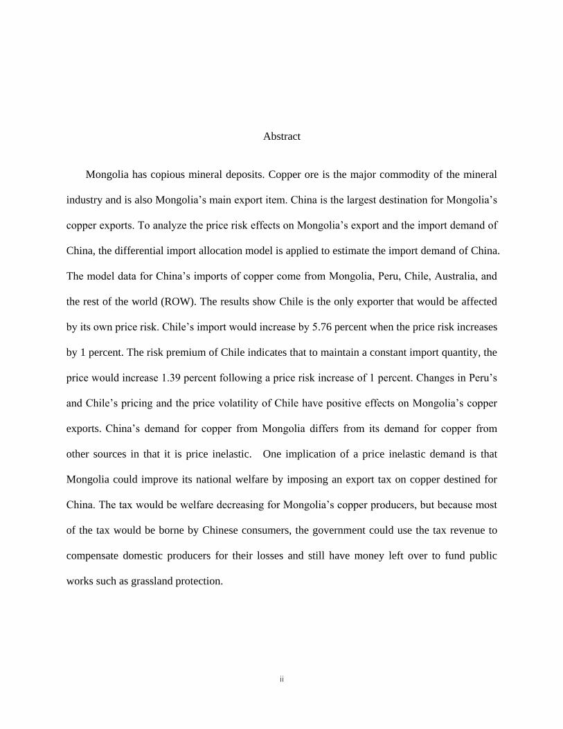
Abstract
Mongolia has copious mineral deposits. Copper ore is the major commodity of the mineral
industry and is also Mongolia’s main export item. China is the largest destination for Mongolia’s
copper exports. To analyze the price risk effects on Mongolia’s export and the import demand of
China, the differential import allocation model is applied to estimate the import demand of China.
The model data for China’s imports of copper come from Mongolia, Peru, Chile, Australia, and
the rest of the world (ROW). The results show Chile is the only exporter that would be affected
by its own price risk. Chile’s import would increase by 5.76 percent when the price risk increases
by 1 percent. The risk premium of Chile indicates that to maintain a constant import quantity, the
price would increase 1.39 percent following a price risk increase of 1 percent. Changes in Peru’s
and Chile’s pricing and the price volatility of Chile have positive effects on Mongolia’s copper
exports. China’s demand for copper from Mongolia differs from its demand for copper from
other sources in that it is price inelastic. One implication of a price inelastic demand is that
Mongolia could improve its national welfare by imposing an export tax on copper destined for
China. The tax would be welfare decreasing for Mongolia’s copper producers, but because most
of the tax would be borne by Chinese consumers, the government could use the tax revenue to
compensate domestic producers for their losses and still have money left over to fund public
works such as grassland protection.
iii
Acknowledgments
I would first like to thank my thesis advisor Dr. Henry Kinnucan of the Agricultural
Economics and Rural Sociology. I still remember the major idea about doing research he told on
class, “Theory”. I learned demand theory in his class, which is the basic theory and guideline for
my research. It is my honor to meet such a patient and professional advisor during my research.
He consistently allowed this paper to be my own work, but steered me in the right the direction
whenever he thought I needed it. I would also like to appreciate my committee member Dr.
Patricia Duffy for the time and support to my research
I would also like to thank my co-advisor, Dr Yaoqi Zhang, who brought me into the
Ecosystems and Societies of Outer and Inner Mongolia project. This project gave me the best
chance to dig deeper in academic fields. Without his passionate participation and input, my
research could not have been successfully completed.
I feel grateful to my friends Meijuan Wang, Mo Zhou, Rui Chen, Chenyu Si for
their keeping company and making my daily life in Auburn memorable.
Finally, I must express my very profound gratitude to my parents for providing me with
unfailing support and continuous encouragement throughout my years of study and through the
process of researching and writing this thesis. This accomplishment would not have been
possible without them. Thank you.
iv
Table of Contents
Abstract ......................................................................................................................................... ii
Acknowledgments........................................................................................................................ iii
List of Tables ................................................................................................................................ v
List of Illustrations ....................................................................................................................... vi
List of Abbreviations .................................................................................................................. vii
Introduction ............................................................................................................................... 1
Literature Review ...................................................................................................................... 4
Model ........................................................................................................................................ 6
Empirical Model ..................................................................................................................... 8
Estimation and Results .............................................................................................................. 9
Summary and Conclusion ....................................................................................................... 18
References ............................................................................................................................... 20
v
List of Tables
Table 1. Summary Statistics for Model Variables: January 2000-September 2012 ................. 11
Table 2. Wald Test for General Restrictions ............................................................................ 12
Table 3. Wald Test for Variance and Covariance Restrictions ................................................. 13
Table 4. Demand Estimates for China Copper Ore Imports ..................................................... 14
Table 5. Demand Elasticities China Copper Ore Imports ......................................................... 16
Table 6. Demand Elasticities for Mongolia Copper Ore Exports ............................................. 17
vi
List of Figures
Figure1. Share of mineral products in Mongolia export ............................................................. 1
Figure 2. Share and value of copper export in Mongolia ............................................................. 2
Figure 3. The allocation of copper import in China .................................................................... 3
Figure 4. Changing of GDP, export and copper price .................................................................. 4
Figure 5. M-GARCH variance estimates: January 2000-September 2012 ................................. 10
vii
List of Abbreviations
DIA Differential Import of Allocation
GDP Gross Domestic Product
M-ARCH Multivariate Autoregressive Conditional Heteroskedasticity
ROW Rest of the World
1
The Effect of Price Risk on Mongolia Copper Export
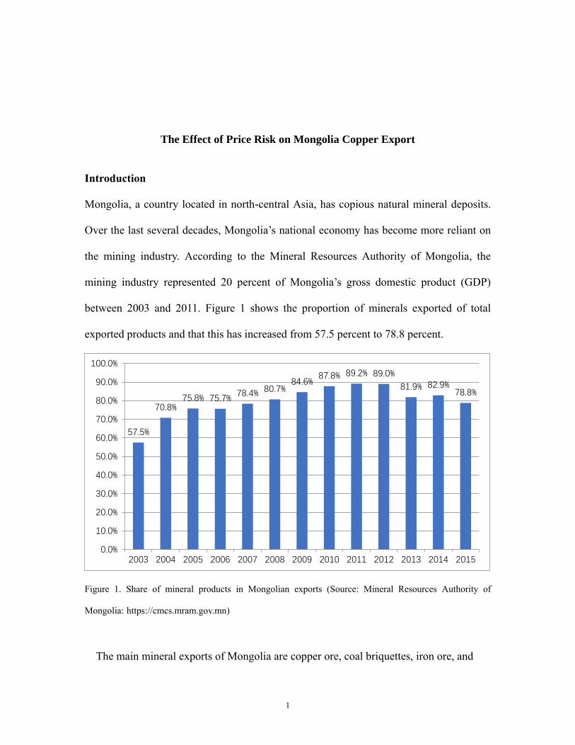
Introduction
Mongolia, a country located in north-central Asia, has copious natural mineral deposits.
Over the last several decades, Mongolia’s national economy has become more reliant on
the mining industry. According to the Mineral Resources Authority of Mongolia, the
mining industry represented 20 percent of Mongolia’s gross domestic product (GDP)
between 2003 and 2011. Figure 1 shows the proportion of minerals exported of total
exported products and that this has increased from 57.5 percent to 78.8 percent.
Figure 1. Share of mineral products in Mongolian exports (Source: Mineral Resources Authority of
Mongolia: https://cmcs.mram.gov.mn)
The main mineral exports of Mongolia are copper ore, coal briquettes, iron ore, and
57.5%
70.8%75.8% 75.7%
78.4% 80.7%84.6%
87.8% 89.2% 89.0%
81.9% 82.9%78.8%
0.0%
10.0%
20.0%
30.0%
40.0%
50.0%
60.0%
70.0%
80.0%
90.0%
100.0%
2003 2004 2005 2006 2007 2008 2009 2010 2011 2012 2013 2014 2015
2
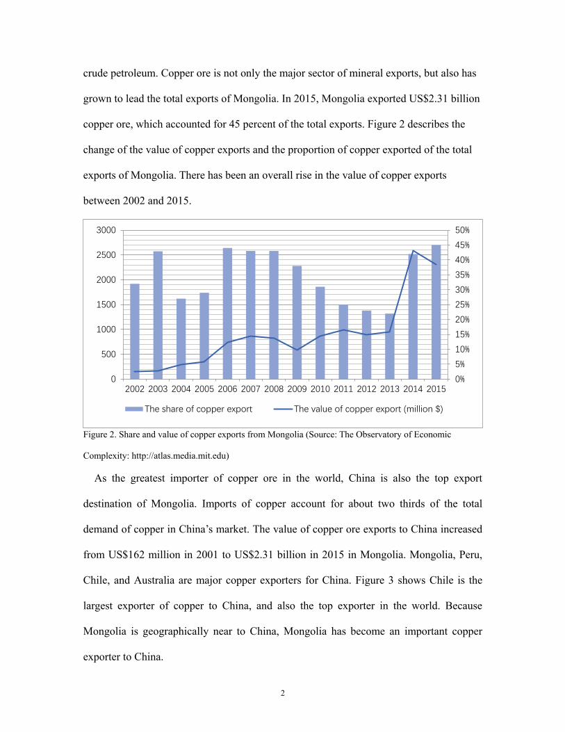
crude petroleum. Copper ore is not only the major sector of mineral exports, but also has
grown to lead the total exports of Mongolia. In 2015, Mongolia exported US$2.31 billion
copper ore, which accounted for 45 percent of the total exports. Figure 2 describes the
change of the value of copper exports and the proportion of copper exported of the total
exports of Mongolia. There has been an overall rise in the value of copper exports
between 2002 and 2015.
Figure 2. Share and value of copper exports from Mongolia (Source: The Observatory of Economic
Complexity: http://atlas.media.mit.edu)
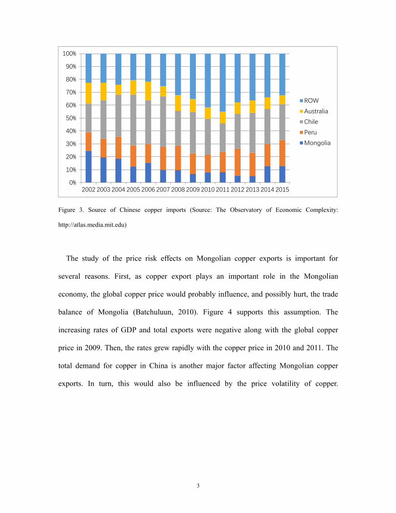
As the greatest importer of copper ore in the world, China is also the top export
destination of Mongolia. Imports of copper account for about two thirds of the total
demand of copper in China’s market. The value of copper ore exports to China increased
from US$162 million in 2001 to US$2.31 billion in 2015 in Mongolia. Mongolia, Peru,
Chile, and Australia are major copper exporters for China. Figure 3 shows Chile is the
largest exporter of copper to China, and also the top exporter in the world. Because
Mongolia is geographically near to China, Mongolia has become an important copper
exporter to China.
0%
5%
10%
15%
20%
25%
30%
35%
40%
45%
50%
0
500
1000
1500
2000
2500
3000
2002 2003 2004 2005 2006 2007 2008 2009 2010 2011 2012 2013 2014 2015
The share of copper export The value of copper export (million $)
3
Figure 3. Source of Chinese copper imports (Source: The Observatory of Economic Complexity:
http://atlas.media.mit.edu)
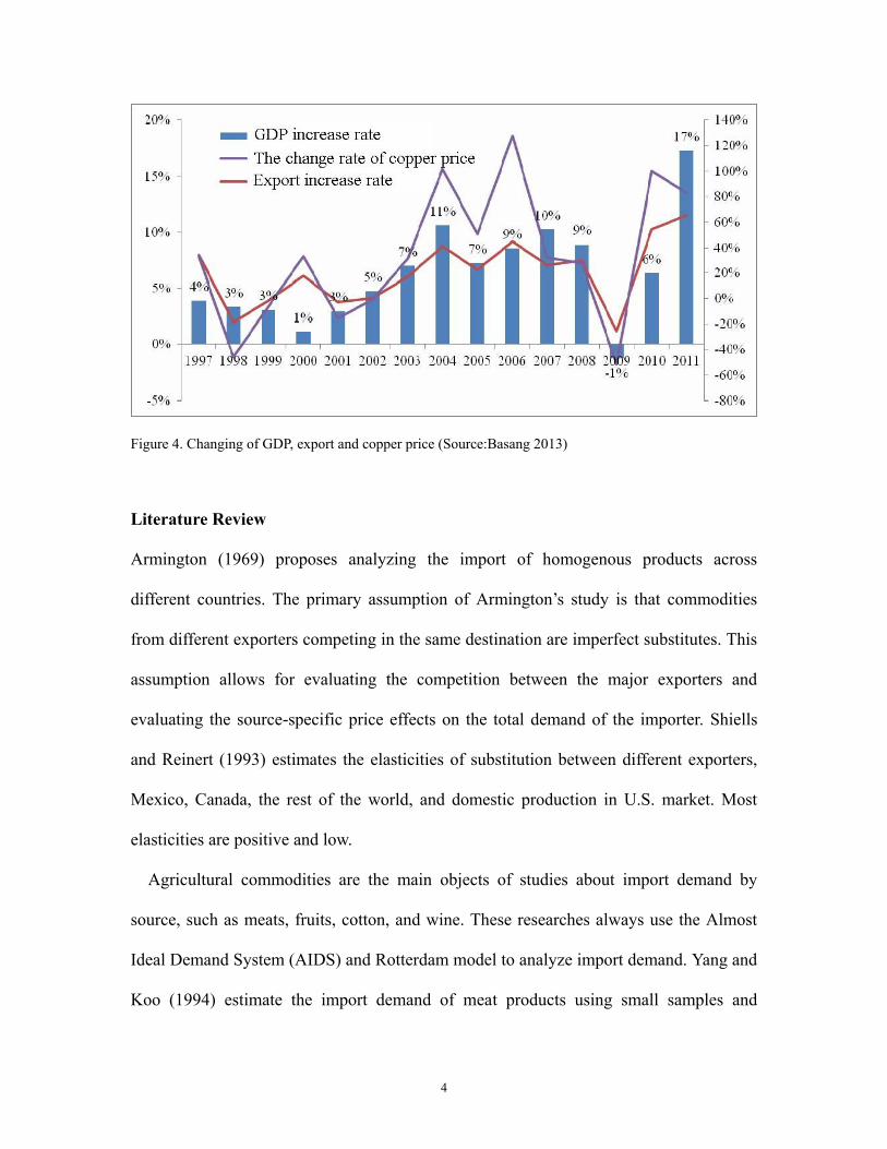
The study of the price risk effects on Mongolian copper exports is important for
several reasons. First, as copper export plays an important role in the Mongolian
economy, the global copper price would probably influence, and possibly hurt, the trade
balance of Mongolia (Batchuluun, 2010). Figure 4 supports this assumption. The
increasing rates of GDP and total exports were negative along with the global copper
price in 2009. Then, the rates grew rapidly with the copper price in 2010 and 2011. The
total demand for copper in China is another major factor affecting Mongolian copper
exports. In turn, this would also be influenced by the price volatility of copper.
0%
10%
20%
30%
40%
50%
60%
70%
80%
90%
100%
2002 2003 2004 2005 2006 2007 2008 2009 2010 2011 2012 2013 2014 2015
ROW
Australia
Chile
Peru
Mongolia
4
Figure 4. Changing of GDP, export and copper price (Source:Basang 2013)
Literature Review
Armington (1969) proposes analyzing the import of homogenous products across
different countries. The primary assumption of Armington’s study is that commodities
from different exporters competing in the same destination are imperfect substitutes. This
assumption allows for evaluating the competition between the major exporters and
evaluating the source-specific price effects on the total demand of the importer. Shiells
and Reinert (1993) estimates the elasticities of substitution between different exporters,
Mexico, Canada, the rest of the world, and domestic production in U.S. market. Most
elasticities are positive and low.
Agricultural commodities are the main objects of studies about import demand by
source, such as meats, fruits, cotton, and wine. These researches always use the Almost
Ideal Demand System (AIDS) and Rotterdam model to analyze import demand. Yang and
Koo (1994) estimate the import demand of meat products using small samples and
5
indicate that the U.S. has the largest potential in the beef market of Japan according to the
AIDS model. Mutondo and Henneberry (2007) describe different exporter performances
in the U.S. meat market and the influences of animal disease on the market. Seale,
Marchant, and Basso (2003) use the AIDS model to estimate the import demand in the
U.S. wine market. Muhammad (2011) analyzes the U.K. import market for wine using
the Rotterdam model. French wine has same performance in U.S. and U.K. markets,
which would attract more revenue with price increases.
Some studies have also focused on the import demand patterns in China. Muhammad,
McPhail, and Kiawu (2012) estimate the import demand of cotton in China and suggest
that if the U.S., as a cotton exporter, increases cotton subsidies it could earn more market
share in the Chinese market. Niquidet and Tang (2013) analyze log and lumber import
demands using the AIDS model and show that the price elasticity of demand is elastic.
Sun (2014) employs the Rotterdam model to assess China’s roundwood import market
and finds there is no obvious competition between the foreign exporters but that a
substitute situation exists. Therefore, research has mostly focused on agricultural and
forestry products. The source diversification analysis of mineral products has received
less attention than other fields.
Nevertheless, the consumption of copper cannot avoid the problem of price risk. The
major factors causing copper price volatility are demand and supply, production costs,
market power, and the forecast of supply and demand (Rosenau-Tornow, Buchholz, and
Riemann 2009). Wolak and Kolstad (1991) indicate that producers attempt to reduce cost
risk by using diversified suppliers. Because mineral products are always treated as inputs
in domestic industry, producers always purchase commodities from different exporters to
6
avoid price risk. This study presents a model to examine the price risk’s effect on import
allocation across different exporters. Does the price risk of foreign copper affect the
allocation of the import market? This is the key problem to figure out in my study.
In previous studies, the impact of price risk on the allocation of the import market has
been estimated. Cavalcanti, Tiago, and Mohaddes (2015) estimates the price volatility of
commodity terms of trade has a significant negative effect on output growth of product
exporters. However, most of studies usually focus on agricultural products. Muhammad
(2015) analyzes the price risk effects on competition in China’s soybean market. The
study indicates that price risk plays an important role in the soybean import market.
Zhang and Zheng (2016) estimate the impact of price risk on the allocation of U.S.
import demand. The study shows that most exporters have significant and negative risk
elasticities, and price stability is important for trade from developing countries to
developed countries. There is an absence of research on the effects of price risk on the
allocation of copper demand. The above studies suggest that the price volatility of import
copper might decrease the trade from exporters.
Model
This study uses Muhammad’s (2012) differential import allocation (DIA) model, which is
derived from the theory of expected utility maximization (Wolak and Kolstad 1991). The
DIA model treats foreign price risk as a factor affecting the optimal allocation of import
across different sources.
Assuming copper is an intermediate good for a firm, the optimal allocation of import
input would be decided in the first stage of a two-stage profit maximization, according to
7
Wolak and Kolstad’s (1991) theory. A firm would decide the output level and domestic
resources for production in the second stage, if the prices of domestic resources and the
amounts of output and import resources have already been known.
R defines the net revenues obtained from outputs and domestic inputs during the
production. 𝑞𝑖 and 𝑝𝑖 represent the quantity and price of import copper from the ith
country (i=1,2…n). The optimal allocation of import demand q would be obtained by the
utility maximization problem:
Max𝑞
𝑈[𝑅𝑡 − 𝐸(𝐩𝑡′ 𝐪𝑡), 𝑉(𝐩𝑡
′ 𝐪𝑡)]
𝑠. 𝑡. 𝑄𝑡 = 𝜄′𝐪𝑡 , 𝐪𝑡 ≥ 0 (1)
E and V represent the function of expectation and variance. p and q are n-dimensional
vectors of the price and quantity of copper import from each exporter. Q is the quantity of
total copper imports and ι is a unit vector. The Lagrangian of (1) is
𝐿 = 𝑈(𝑅𝑡 − �̃�′𝐪, 𝐪′𝛀𝐪) + 𝜆(𝑄 − 𝜄′𝐪) (2)
where �̃� = 𝐸(𝑝) and 𝛺 = 𝐸{(𝑝 − �̃�)(𝑝 − �̃�)′} , �̃� and 𝛀 represent the conditional
expectation and variance of import price p. 𝜆 is Lagrange multiplier on the constraint.
The first order condition from equation (2) with respect to the ith copper import is:
𝐿𝑖 =𝜕𝐿
𝜕𝑞𝑖= −𝑈1�̃�𝑖 + 2𝑈2(𝑞𝑖𝜎𝑖
2 + ∑ 𝑞𝑗𝜎𝑖𝑗𝑗≠𝑖 ) − 𝜆 = 0 (3)
Where the derivatives of maximum utility U with respect to the ith argument are
represented by 𝑈𝑖 . 𝜎𝑖2 means conditional variance and 𝜎𝑖𝑗 means conditional
covariance of import price. Equation (4) is the fundamental mode of total import demand
function.
8
𝑞𝑖∗ = 𝑞𝑖(𝑄, �̃�1, �̃�2, … , �̃�𝑛, 𝜎1
2, 𝜎22, … , 𝜎𝑛
2,
𝜎12, … , 𝜎1,𝑛, 𝜎23, … , 𝜎2,𝑛, … , 𝜎𝑛−1,𝑛). (4)
For example, if n=5 this means each equation in the system contains 10 covariance
variables as follows 𝜎12, 𝜎13, 𝜎14, 𝜎15, 𝜎23, 𝜎24, 𝜎25, 𝜎34, 𝜎35, 𝜎45.
Following Theil’s (1977,1980) studies, the differential approach is used to derive the
import demand model. The total differential of equation (4) is:
𝑑𝑞𝑖 =𝜕𝑞𝑖
𝜕𝑄𝑑𝑄 + ∑
𝜕𝑞𝑖
𝜕�̃�𝑗𝑑�̃�𝑗
𝑛𝑗=1 + ∑
𝜕𝑞𝑖
𝜕𝜎𝑗2 𝑑𝜎𝑗
2𝑛𝑗=1 + ∑ ∑
𝜕𝑞𝑖
𝜕𝜎𝑔ℎ𝑑𝜎𝑔ℎℎ≠𝑔
ℎ>𝑔𝑔≠ℎ (5)
After some transformation steps from equation (5), the DIA model in
logarithmic-differential form is obtained:
𝑠𝑖𝑑 log 𝑞𝑖 =𝜕𝑞𝑖
𝜕𝑄𝑑 log 𝑄 + 𝑠𝑖 ∑
𝜕 log 𝑞𝑖
𝜕 log �̃�𝑗
𝑛
𝑗=1
𝑑 log �̃�𝑗 + 𝑠𝑖 ∑𝜕 log 𝑞𝑖
𝜕 log 𝜎𝑗2
𝑛
𝑗=1
𝑑 log 𝜎𝑗2
+𝑠𝑖 ∑ ∑𝜕 log 𝑞𝑖
𝜕 log 𝜎𝑔ℎ𝑑 log 𝜎𝑔ℎℎ≠𝑔
ℎ>𝑔𝑔≠ℎ (6)
where 𝑠𝑖 = 𝑞𝑖/𝑄 is the share of total imports from country i. 𝜕𝑞𝑖/𝜕𝑄>0 is expected,
which implies increasing in total imports would increase the imports from exporter i.
𝑠𝑖𝜕 log 𝑞𝑖 /𝜕 log �̃�𝑖 should be negative, which are consistent with the demand theory.
When ≠ 𝑗 , the positive sign of 𝑠𝑖𝜕 log 𝑞𝑖 /𝜕 log �̃�𝑗 would represent the imports from
exporter i and j are substitutes. In contrast, the imports are complements. 𝑠𝑖𝜕 log 𝑞𝑖 /
𝜕 log 𝜎𝑗2, which represents the variance effect, could be positive or negative depending on
the importers’ response of price risk. 𝑠𝑖𝜕 log 𝑞𝑖 /𝜕 log 𝜎𝑔ℎ reflects the competitive
relationship between the any two importers and they are possible to be negative or
positive.
9
Empirical Model
The DIA model contains five equations as follows:
�̅�𝑖,𝑡∆𝑞𝑖,𝑡 = 𝜃𝑖∆𝑄𝑡∗ + ∑ 𝜋𝑖𝑗∆�̃�𝑗,𝑡
5
𝑗=1
+ ∑ 𝑣𝑖𝑗∆𝜎𝑗,𝑡2
5
𝑗=1
+ ∑ ∑ 𝜔𝑖𝑔ℎ∆𝜎𝑔ℎ,𝑡
ℎ≠𝑔ℎ>𝑔
𝑔≠ℎ
+ ε𝑖,𝑡 𝑖
= 1, … ,5
(7)
The matrix of coefficients corresponding to the price and variance terms are 5x5 while
the matrix of coefficients corresponding to the covariance terms is 5x10. For easily
estimating the log change, first differences are used where for any variable x, 𝑑 𝑙𝑜𝑔 𝑥𝑡 ≈
∆𝑥𝑡 = 𝑙𝑛(𝑥𝑡) − 𝑙𝑛(𝑥𝑡−1). The variable of market share is estimated by the average of
two sequential periods, �̅�𝑖,𝑡 = 0.5(𝑠𝑖,𝑡 + 𝑠𝑖,𝑡−1) . To ensure the import constraints
∑ sid log qini=1 = d log Q are satisfied in empirical procedure, ∆𝑄𝑡 = 𝑙𝑛(𝑄𝑡) − 𝑙𝑛(𝑄𝑡−1)
is replaced by ∆𝑄𝑡∗ = ∑ s̅i,t∆𝑞𝑖,𝑡
𝑛𝑖=1 .
θi represents the marginal market share effects on copper import from country i. 𝜋𝑖𝑗
reflects the price effects on copper import from country i. It reflects the own price effect
when 𝑖 = 𝑗 and the cross price effect when 𝑖 ≠ 𝑗 . 𝑣𝑖𝑗 shows the variance effect.
𝜔𝑖𝑔ℎ means the covariance effect. The general restrictions of demand theory are assumed
to be satisfied in the DIA model. These restrictions are the following conditions:
∑ 𝜃𝑖𝑛𝑖=1 = 1; ∑ 𝜋𝑖𝑗
𝑛𝑖=1 = 0; ∑ 𝑣𝑖𝑗
𝑛𝑖=1 = 0; ∑ 𝜔𝑖𝑔ℎ
𝑛𝑖=1 = 0; ∑ 𝜋𝑖𝑗
𝑛𝑗=1 = 0; and 𝜋𝑖𝑗 = 𝜋𝑗𝑖.
To derive the specific total import, price, risk and covariance elasticities from equation
(7), these following methods are applied:
10
𝜂𝑖 = 𝑑 log 𝑞𝑖 𝑑 log 𝑄⁄ = 𝜃𝑖/�̅�𝑖 (8)
𝜂ij = 𝑑 log 𝑞𝑖 𝑑 log �̃�𝑖⁄ = 𝜋𝑖𝑗/�̅�𝑖 (9)
𝜂𝑖𝑗𝜎 = 𝑑 log 𝑞𝑖 𝑑 log 𝜎𝑖
2⁄ = 𝑣𝑖𝑗/�̅�𝑖 (10)
𝜂𝑖𝑔ℎ𝜎 = 𝑑 log 𝑞𝑖 𝑑 log 𝜎𝑔ℎ⁄ = 𝜔𝑖𝑔ℎ/�̅�𝑖 (11)
In Wolak and Kolstad’s (1991) study, the risk premium is defined as the negative value of
the risk elasticity of copper imports with respect to price elasticity:
𝑅𝑃𝑖 = − 𝑑 log �̃�𝑖 𝑑 log 𝜎𝑖2⁄ = −𝑣𝑖𝑗/𝜋𝑖𝑗 (12)
Risk premium is used to estimate the impact of price risk on the price change under the
consistent import allocation, which measures the exporter i seems willing to pay how
much higher above the current price for the import of copper having no price risk.
According Wolak and Kolstad (1991), the expected sign of risk premium is positive.
Estimation and Results
This paper uses the monthly data (January 2000–December 2006 and January 2010–
September 2012) provided by the General Administration of Customs of the People’s
Republic of China and defined according to the HS classification 2603: copper ores and
concentrates. The following exporting countries are considered for the analysis: Mongolia,
Peru, Chile, Australia, and the rest of the world (ROW). The ROW is an aggregation of
all countries not specified.
To obtain the conditional expectation, variance, and covariance of copper import prices,
the following autoregressive equation is estimated assuming a multivariate GARCH (1,1)
process (Appelbaum and Woodland 2010):
11
∆𝐩𝒕 =∝𝟎+ 𝑨𝟏∆𝒑𝒕−𝟏 + 𝑨𝟐∆𝒛𝒕 + 𝜺𝒕 (12)
�̂�𝒕 = 𝑩𝟎 + 𝑩𝟏𝜺𝒕−𝟏𝜺𝒕′𝑩𝟏 + 𝑩𝟐�̂�𝒕−𝟏𝑩𝟐 (13)
where ∆pt represents the first difference of the logarithm of the import price. Ω̂ defines
the estimated variance and covariance matrix. In this model, equation (12) and (13) are
the mean equation and variance equation for price change. The conditional variance
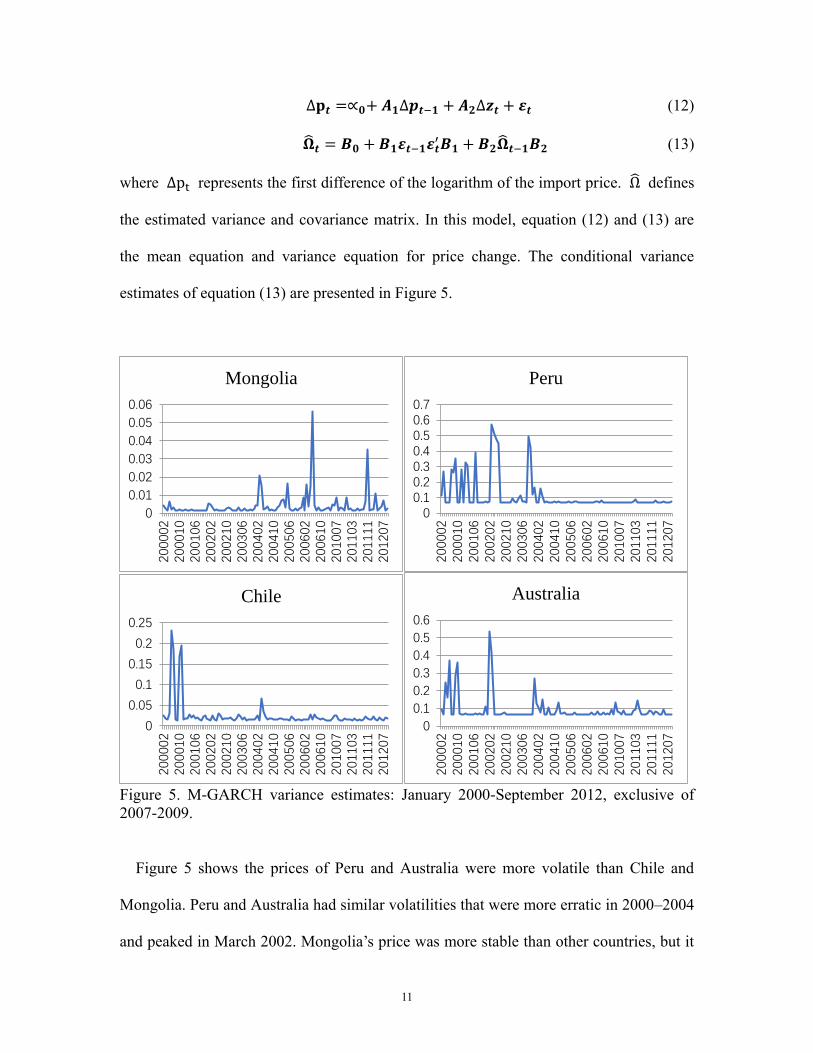
estimates of equation (13) are presented in Figure 5.
Figure 5. M-GARCH variance estimates: January 2000-September 2012, exclusive of
2007-2009.
Figure 5 shows the prices of Peru and Australia were more volatile than Chile and
Mongolia. Peru and Australia had similar volatilities that were more erratic in 2000–2004
and peaked in March 2002. Mongolia’s price was more stable than other countries, but it
0
0.01
0.02
0.03
0.04
0.05
0.06
20000
220001
020010
620020
220021
020030
620040
220041
020050
620060
220061
020100
720110
320111
120120
7Mongolia
00.10.20.30.40.50.60.7
20000
220001
020010
620020
220021
020030
620040
220041
020050
620060
220061
020100
720110
320111
120120
7
Peru
0
0.05
0.1
0.15
0.2
0.25
200002
200010
200106
200202
200210
200306
200402
200410
200506
200602
200610
201007
201103
201111
201207
Chile
0
0.1
0.2
0.3
0.4
0.5
0.6
200002
200010
200106
200202
200210
200306
200402
200410
200506
200602
200610
201007
201103
201111
201207
Australia
12
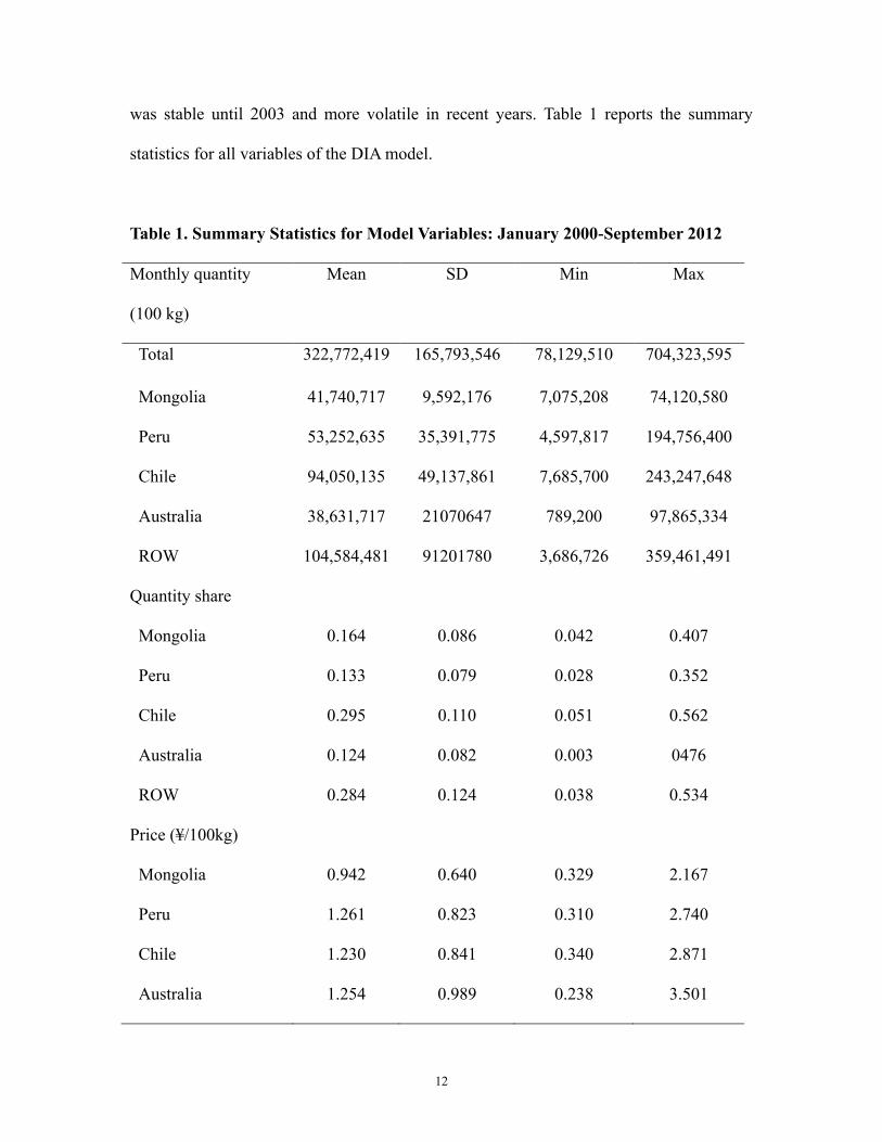
was stable until 2003 and more volatile in recent years. Table 1 reports the summary
statistics for all variables of the DIA model.
Table 1. Summary Statistics for Model Variables: January 2000-September 2012
Monthly quantity
(100 kg)
Mean SD Min Max
Total 322,772,419 165,793,546 78,129,510 704,323,595
Mongolia 41,740,717 9,592,176 7,075,208 74,120,580
Peru 53,252,635 35,391,775 4,597,817 194,756,400
Chile 94,050,135 49,137,861 7,685,700 243,247,648
Australia 38,631,717 21070647 789,200 97,865,334
ROW 104,584,481 91201780 3,686,726 359,461,491
Quantity share
Mongolia 0.164 0.086 0.042 0.407
Peru 0.133 0.079 0.028 0.352
Chile 0.295 0.110 0.051 0.562
Australia 0.124 0.082 0.003 0476
ROW 0.284 0.124 0.038 0.534
Price (¥/100kg)
Mongolia 0.942 0.640 0.329 2.167
Peru 1.261 0.823 0.310 2.740
Chile 1.230 0.841 0.340 2.871
Australia 1.254 0.989 0.238 3.501
13
ROW 1.105 0.696 0.164 2.583
Variance of price
Mongolia 0.0034 0.0033 0.0017 0.0271
Peru 0.1210 0.1377 0.0603 0.6883
Chile 0.0184 0.0311 0.0095 0.2735
Australia 0.0917 0.0739 0.0641 0.5426
ROW 0.0341 0.0361 0.0229 0.2960
Covariance of price
Mongolia–Peru 0.0064 0.0088 -0.0113 0.0442
Mongolia–Chile 0.0009 0.0020 -0.0003 0.0119
Mongolia–Australia -0.0018 0.0074 -0.0580 0.0175
Mongolia–ROW 0.0019 0.0029 -0.0033 0.0193
Peru–Chile -0.0003 0.4007 -0.0639 0.3377
Peru–Australia -0.0234 0.0757 -0.5534 0.0079
Peru–ROW -0.0162 0.0724 -0.4751 0.0722
Chile–Australia -0.0020 0.0306 -0.1824 0.0094
Chile–ROW -0.0053 0.0172 -0.1313 0.0201
Australia–ROW -0.0005 0.0131 -0.0607 0.0757
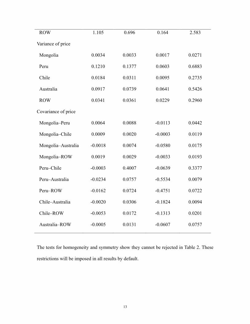
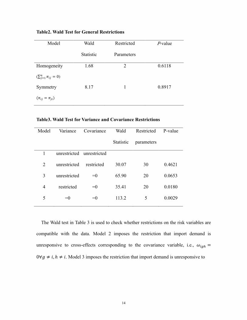
The tests for homogeneity and symmetry show they cannot be rejected in Table 2. These
restrictions will be imposed in all results by default.
14
Table2. Wald Test for General Restrictions
Model Wald
Statistic
Restricted
Parameters
P-value
Homogeneity
(∑ 𝜋𝑖𝑗𝑛𝑗=1 = 0)
1.68 2 0.6118
Symmetry
(𝜋𝑖𝑗 = 𝜋𝑗𝑖)
8.17 1 0.8917
Table3. Wald Test for Variance and Covariance Restrictions
Model Variance Covariance Wald
Statistic
Restricted
parameters
P-value
1 unrestricted unrestricted
2 unrestricted restricted 30.07 30 0.4621
3 unrestricted =0 65.90 20 0.0653
4 restricted =0 35.41 20 0.0180
5 =0 =0 113.2 5 0.0029
The Wald test in Table 3 is used to check whether restrictions on the risk variables are
compatible with the data. Model 2 imposes the restriction that import demand is
unresponsive to cross-effects corresponding to the covariance variable, i.e., 𝜔𝑖𝑔ℎ =
0∀𝑔 ≠ 𝑖, ℎ ≠ 𝑖. Model 3 imposes the restriction that import demand is unresponsive to
15
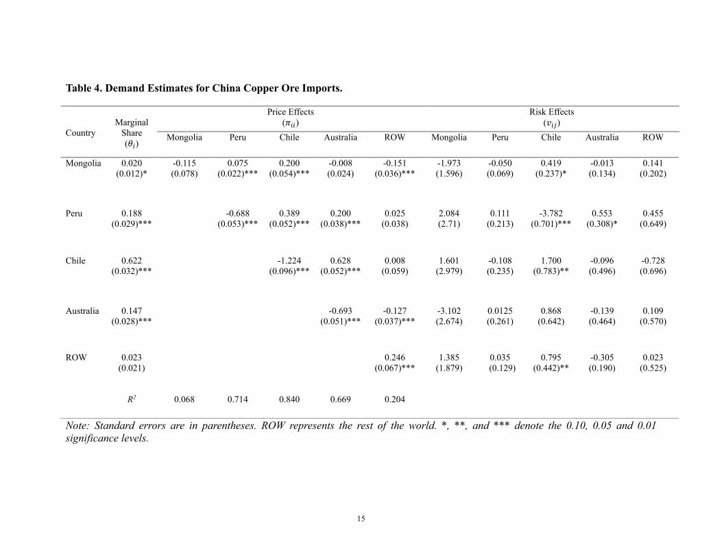
Table 4. Demand Estimates for China Copper Ore Imports.
Note: Standard errors are in parentheses. ROW represents the rest of the world. *, **, and *** denote the 0.10, 0.05 and 0.01
significance levels.
Country
Marginal
Share
(𝜃𝑖)
Price Effects
(𝜋𝑖𝑖)
Risk Effects
(𝑣𝑖𝑗)
Mongolia Peru Chile Australia ROW Mongolia Peru Chile Australia ROW
Mongolia 0.020
(0.012)*
-0.115
(0.078)
0.075
(0.022)***
0.200
(0.054)***
-0.008
(0.024)
-0.151
(0.036)***
-1.973
(1.596)
-0.050
(0.069)
0.419
(0.237)*
-0.013
(0.134)
0.141
(0.202)
Peru 0.188
(0.029)***
-0.688
(0.053)***
0.389
(0.052)***
0.200
(0.038)***
0.025
(0.038)
2.084
(2.71)
0.111
(0.213)
-3.782
(0.701)***
0.553
(0.308)*
0.455
(0.649)
Chile 0.622
(0.032)***
-1.224
(0.096)***
0.628
(0.052)***
0.008
(0.059)
1.601
(2.979)
-0.108
(0.235)
1.700
(0.783)**
-0.096
(0.496)
-0.728
(0.696)
Australia 0.147
(0.028)***
-0.693
(0.051)***
-0.127
(0.037)***
-3.102
(2.674)
0.0125
(0.261)
0.868
(0.642)
-0.139
(0.464)
0.109
(0.570)
ROW 0.023
(0.021)
0.246
(0.067)***
1.385
(1.879)
0.035
(0.129)
0.795
(0.442)**
-0.305
(0.190)
0.023
(0.525)
R2 0.068 0.714 0.840 0.669 0.204
16
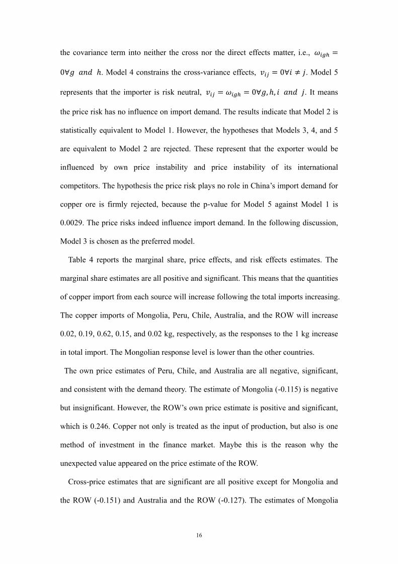
the covariance term into neither the cross nor the direct effects matter, i.e., 𝜔𝑖𝑔ℎ =
0∀𝑔 𝑎𝑛𝑑 ℎ. Model 4 constrains the cross-variance effects, 𝑣𝑖𝑗 = 0∀𝑖 ≠ 𝑗. Model 5
represents that the importer is risk neutral, 𝑣𝑖𝑗 = 𝜔𝑖𝑔ℎ = 0∀𝑔, ℎ, 𝑖 𝑎𝑛𝑑 𝑗. It means
the price risk has no influence on import demand. The results indicate that Model 2 is
statistically equivalent to Model 1. However, the hypotheses that Models 3, 4, and 5
are equivalent to Model 2 are rejected. These represent that the exporter would be
influenced by own price instability and price instability of its international
competitors. The hypothesis the price risk plays no role in China’s import demand for
copper ore is firmly rejected, because the p-value for Model 5 against Model 1 is
0.0029. The price risks indeed influence import demand. In the following discussion,
Model 3 is chosen as the preferred model.
Table 4 reports the marginal share, price effects, and risk effects estimates. The
marginal share estimates are all positive and significant. This means that the quantities
of copper import from each source will increase following the total imports increasing.
The copper imports of Mongolia, Peru, Chile, Australia, and the ROW will increase
0.02, 0.19, 0.62, 0.15, and 0.02 kg, respectively, as the responses to the 1 kg increase
in total import. The Mongolian response level is lower than the other countries.
The own price estimates of Peru, Chile, and Australia are all negative, significant,
and consistent with the demand theory. The estimate of Mongolia (-0.115) is negative
but insignificant. However, the ROW’s own price estimate is positive and significant,
which is 0.246. Copper not only is treated as the input of production, but also is one
method of investment in the finance market. Maybe this is the reason why the
unexpected value appeared on the price estimate of the ROW.
Cross-price estimates that are significant are all positive except for Mongolia and
the ROW (-0.151) and Australia and the ROW (-0.127). The estimates of Mongolia
17
and Chile, Mongolia and Australia, Peru and the ROW, and Chile and the ROW are
insignificant. Chile is the only country that has a significant own risk estimate (1.700).
The value of Chile’s own risk estimate exceeds the absolute value of Chile’s own
price estimate. This means imports from Chile would have more response to price
risk.
Only four of all cross-price risks estimates are significant. They are the coefficients
of Chile with respect to Mongolia (0.419), Peru (-3.782), and the ROW (0.795), and
Australia with respect to Peru (0.553). This means the imports from Mongolia and the
ROW will increase when the import price of Chile becomes more volatile, but the
imports from Peru will decrease. Imports from Peru have an inverse effect on
Australia’s price.
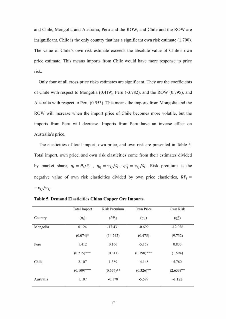
The elasticities of total import, own price, and own risk are presented in Table 5.
Total import, own price, and own risk elasticities come from their estimates divided
by market share, 𝜂𝑖 = 𝜃𝑖/�̅�𝑖 , 𝜂ij = 𝜋𝑖𝑗/�̅�𝑖 , 𝜂𝑖𝑗𝜎 = 𝑣𝑖𝑗/�̅�𝑖 . Risk premium is the
negative value of own risk elasticities divided by own price elasticities, 𝑅𝑃𝑖 =
−𝑣𝑖𝑗/𝜋𝑖𝑗.
Table 5. Demand Elasticities China Copper Ore Imports.
Country
Total Import
(𝜂𝑖)
Risk Premium
(𝑅𝑃𝑖)
Own Price
(𝜂𝑖𝑖)
Own Risk
(𝜂𝑖𝑖𝜎)
Mongolia 0.124
(0.074)*
-17.431
(14.242)
-0.699
(0.475)
-12.036
(9.732)
Peru 1.412
(0.215)***
0.166
(0.311)
-5.159
(0.398)***
0.833
(1.594)
Chile 2.107
(0.109)***
1.389
(0.676)**
-4.148
(0.326)**
5.760
(2.653)**
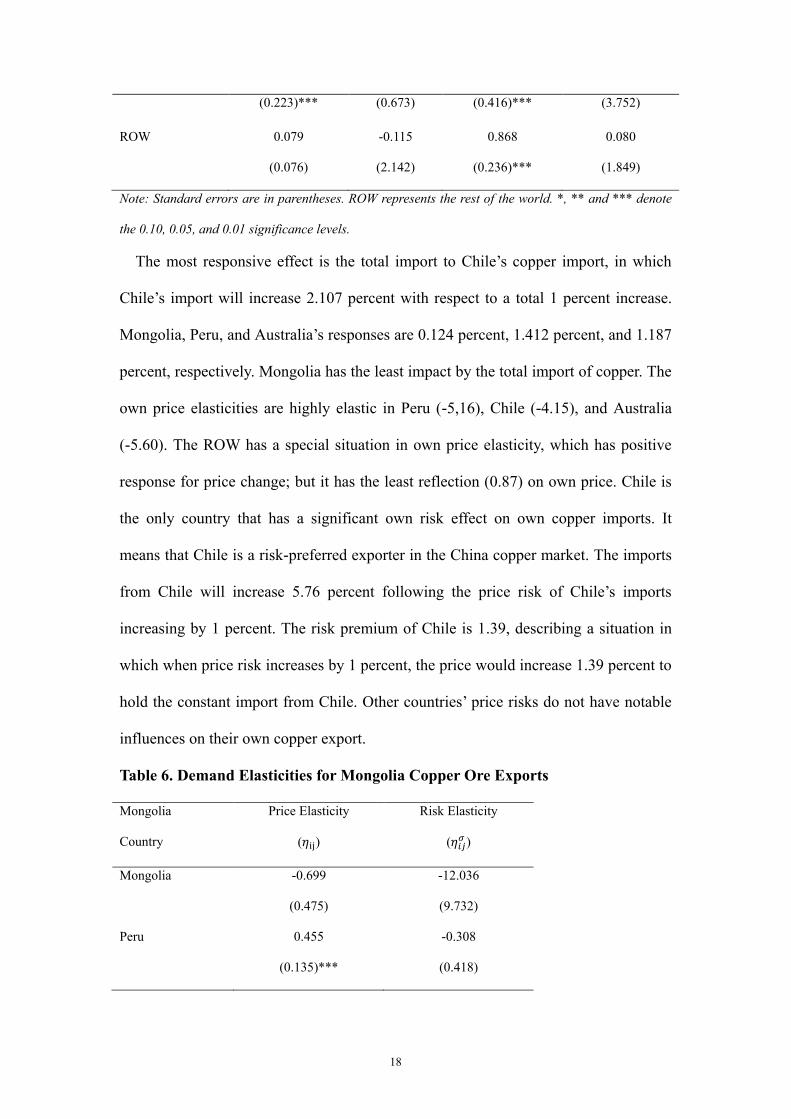
Australia 1.187 -0.178 -5.599 -1.122
18
(0.223)*** (0.673) (0.416)*** (3.752)
ROW 0.079
(0.076)
-0.115
(2.142)
0.868
(0.236)***
0.080
(1.849)
Note: Standard errors are in parentheses. ROW represents the rest of the world. *, ** and *** denote
the 0.10, 0.05, and 0.01 significance levels.
The most responsive effect is the total import to Chile’s copper import, in which
Chile’s import will increase 2.107 percent with respect to a total 1 percent increase.
Mongolia, Peru, and Australia’s responses are 0.124 percent, 1.412 percent, and 1.187
percent, respectively. Mongolia has the least impact by the total import of copper. The
own price elasticities are highly elastic in Peru (-5,16), Chile (-4.15), and Australia
(-5.60). The ROW has a special situation in own price elasticity, which has positive
response for price change; but it has the least reflection (0.87) on own price. Chile is
the only country that has a significant own risk effect on own copper imports. It
means that Chile is a risk-preferred exporter in the China copper market. The imports
from Chile will increase 5.76 percent following the price risk of Chile’s imports
increasing by 1 percent. The risk premium of Chile is 1.39, describing a situation in
which when price risk increases by 1 percent, the price would increase 1.39 percent to
hold the constant import from Chile. Other countries’ price risks do not have notable
influences on their own copper export.
Table 6. Demand Elasticities for Mongolia Copper Ore Exports
Mongolia
Country
Price Elasticity
(𝜂ij)
Risk Elasticity
(𝜂𝑖𝑗𝜎 )
Mongolia -0.699
(0.475)
-12.036
(9.732)
Peru 0.455
(0.135)***
-0.308
(0.418)

19
Chile 1.217
(0.330)***
2.554
(1.444)*
Australia -0.050
(0.145)
-0.079
(0.818)
ROW -0.823
(0.219)***
0.862
(1.233)
Note: Standard errors are in parentheses. ROW represents the rest of the world. *, **, and *** denote
the 0.10, 0.05 and 0.01 significance levels.
Table 6 shows the performance of Mongolian copper exports with respect to the other
exporters. Mongolia’s own price elasticity is insignificant, but the value is negative
and consistent to demand theory. The cross-price elasticities of Mongolia and Peru
(0.46), and Mongolia and Chile (1.22) are positive. This denotes that the import
copper of Mongolia and Peru, and Chile are substitute. The copper price of Mongolia
is more sensitive with the price of Chile than with the price of Peru. The import
copper of Mongolia and the ROW are complementary goods. Chile is the only
exporter whose price risk has positive and significant effects on the copper imports
from Mongolia. The imports from Mongolia would change 2.55 percent in the same
trend while Chile changes 1 percent. The impact of Chile’s price risk also exceeds
Chile’s price effect.
Summary and Conclusion
This study uses the source disaggregated demand system to analyze the price risk
effects on the import market. As a great part of Mongolia’s national economy, it is
valuable to gain insight into copper export’s condition. Because most of Mongolia’s
copper is exported to the Chinese market and Mongolia also is one of the major
exporters in this market, the import demand of China is used to apply the source
disaggregated demand model. Following Muhammad’s (2012) DIA model and
20
evaluating the data of other main exporters in China’s copper market, the conditional
variances and covariances that represent the variables of price risk are obtained
through the multivariate GARCH (1,1) process. Then Wald tests are used to determine
the best model fitting the data. The test results show that unrelated covariate effects on
copper imports from each source are insignificant. Finally, the elasticities of total
import quantity, price, price risk, and risk premium are reported in the results.
In the Chinese market, Peru, Chile, and Australia are highly sensitive to own prices
on their copper export quantities. As the top copper exporter for China and the world,
Chile also has the characteristics that will be most affected by the total imports of
China and prefers more price volatility. The only significant risk premium is for
Chile’s copper exports. The positive value 1.39 shows that the copper imports from
Chile are more sensitive to price risk than the change of copper price. Mongolia is a
relatively stable source for the copper imports of China.
The demand of Mongolian copper import is highly price inelastic, which might be
caused by policy instability, unpredictability, and non-transparency in Mongolia. The
changes of Peru, Chile, and the ROW’s price and Chile’s price volatility are the
significant factors for Mongolia’s copper ore export. The relations between
Mongolia’s copper and Peru and Chile’s copper are substitutes. Chile’s volatility
would encourage the copper export of Mongolia. Own price change and own price
risk do not have powerful impacts on Mongolia’s copper export.
21
References
Armington P S. A theory of demand for products distinguished by place of
production[J]. Staff Papers, 1969, 16(1): 159-178.
Appelbaum E, Woodland A D. The effects of foreign price uncertainty on Australian
production and trade[J]. Economic Record, 2010, 86(273): 162-177.
Batchuluun A, Lin J Y. An analysis of mining sector economics in Mongolia[J]. 2010.
Basang B. Natural resources and Mongolian ecocomic growth[D].2013
General Administration of Customs of the People’s Republic of China(GACC).2017.
http://www.customs.gov.cn/
Muhammad A. Wine demand in the United Kingdom and new world structural change:
a source‐disaggregated analysis[J]. Agribusiness, 2011, 27(1): 82-98.
Muhammad A, McPhail L, Kiawu J. Do US cotton subsidies affect competing
exporters? An analysis of import demand in China[J]. Journal of Agricultural and
Applied Economics, 2012, 44(2): 235-249.
Muhammad A. Source diversification and import price risk[J]. American journal of
agricultural economics, 2012, 94(3): 801-814.
Muhammad A. Price risk and exporter competition in China's soybean market[J].
Agribusiness, 2015, 31(2): 188-197.
Mutondo J E, Henneberry S R. A source-differentiated analysis of US meat demand[J].
Journal of Agricultural and Resource Economics, 2007: 515-533.
Niquidet K, Tang J. Elasticity of demand for Canadian logs and lumber in China and
Japan[J]. Canadian journal of forest research, 2013, 43(12): 1196-1202.
Rosenau-Tornow D, Buchholz P, Riemann A, et al. Assessing the long-term supply
22
risks for mineral raw materials—a combined evaluation of past and future
trends[J]. Resources Policy, 2009, 34(4): 161-175.
Seale Jr J L, Marchant M A, Basso A. Imports versus domestic production: A demand
system analysis of the US red wine market[J]. Review of Agricultural Economics,
2003, 25(1): 187-202.
Shiells C R, Reinert K A. Armington models and terms-of-trade effects: some
econometric evidence for North America[J]. Canadian Journal of Economics,
1993: 299-316.
Sun C. Recent growth in China's roundwood import and its global implications[J].
Forest Policy and Economics, 2014, 39: 43-53.
Theil H. The independent inputs of production[J]. Econometrica: Journal of the
Econometric Society, 1977: 1303-1327.
Theil H. The Systemwide Approach to Microeconomics[J]. University of Chicago
Press Economics Books, 1980.
Wolak F A, Kolstad C D. A model of homogeneous input demand under price
uncertainty[J]. The American Economic Review, 1991: 514-538.
Yang S R, Koo W W. Japanese meat import demand estimation with the source
differentiated AIDS model[J]. Journal of Agricultural and Resource Economics,
1994: 396-408.
Zhang D, Zheng Y. The role of price risk in China’s agricultural and fisheries exports
to the US[J]. Applied Economics, 2016, 48(41): 3944-3960.