Munich Personal RePEc Archive

The Effect of Traffic Safety Laws and

Obesity Rates on Living Organ

Donations

Fernandez, Jose and Stohr, Lisa

University of Louisville, University of Louisivlle

31 August 2009

Online at https://mpra.ub.uni-muenchen.de/17033/

MPRA Paper No. 17033, posted 01 Sep 2009 07:43 UTC

The Effect of Traffic Safety Laws and Obesity

Rates on Living Organ Donations

Jose M. Fernandez University of Louisville

Lisa Stohr

Louisville, KY

8/31/2009

Abstract:

This paper uses variation in traffic safety laws and obesity rates to identify substitution patterns between living and cadaveric kidney donors. Using panel data from 1988-2008, we find that a 1% decrease in the supply of cadaveric donors per 100,000 increases the supply of living donors per 100,000 by .7%. With respect to traffic safety laws, a national adoption of partial helmet laws is estimated to decrease cadaveric donors by 6%, but leads to a 4.2% increase in the number of living donors, or a net effect of 1.8% decrease in the supply of kidney donations. The recent rise in obesity rates is estimated to increase living donor rates by roughly 18%. Lastly, we find evidence that increases in disposable income per capita is associated with an increase in the number of non-biological living donors within a state, but is not found to have an effect on biological donor rates.

1

1. Introduction

On April 21st 2008, there were 101,687 patients awaiting an organ transplant, but only

27,958 transplants were performed in that year.1 The critical shortage of organs is the result of

an artificial price ceiling instituted by the National Organ Transplant Act of 1984, which makes

financial compensation for organs unlawful. For this reason, the current supply of organs is

generated by cadaveric and altruistic living donors.

The number of living donors has increased dramatically from 1,769 in 1988 to 5,955 in

2008 or an increase of 237% (as seen in Figure 1). Over the same period, the ratio of

biological donors to living donors has decreased from 93% to 60%. Although the shortage of

organs for donation has received considerable attention in both the academic literature and the

press, there is still little empirical evidence identifying potential causes for the increase in

living donor rates, the trade-offs between living and cadaveric donors, and the change in living

donor composition from primarily biological donors to a substantial increase in non-biological

donors.

In this paper we consider the effect that motor vehicle safety laws and the growing

obesity epidemic has on the supply of living donors. Unlike cadaveric donors where the

functional value of the organ to the donor is small, living donors must consider the potential

long term healthcare cost associated with donating an organ. These costs include an increase

in both mortality and morbidity risk, lost wages generated by time away from work during

recovery, and possibly long term poor health. Potential living donors must weigh these costs

and benefits conditional on alternative sources of organs (cadaveric organs and other living

donors) as well as increases in the demand for organs.

1 Based on OPTN data as of March 13, 2009. See http://www.optn.org/ .

2

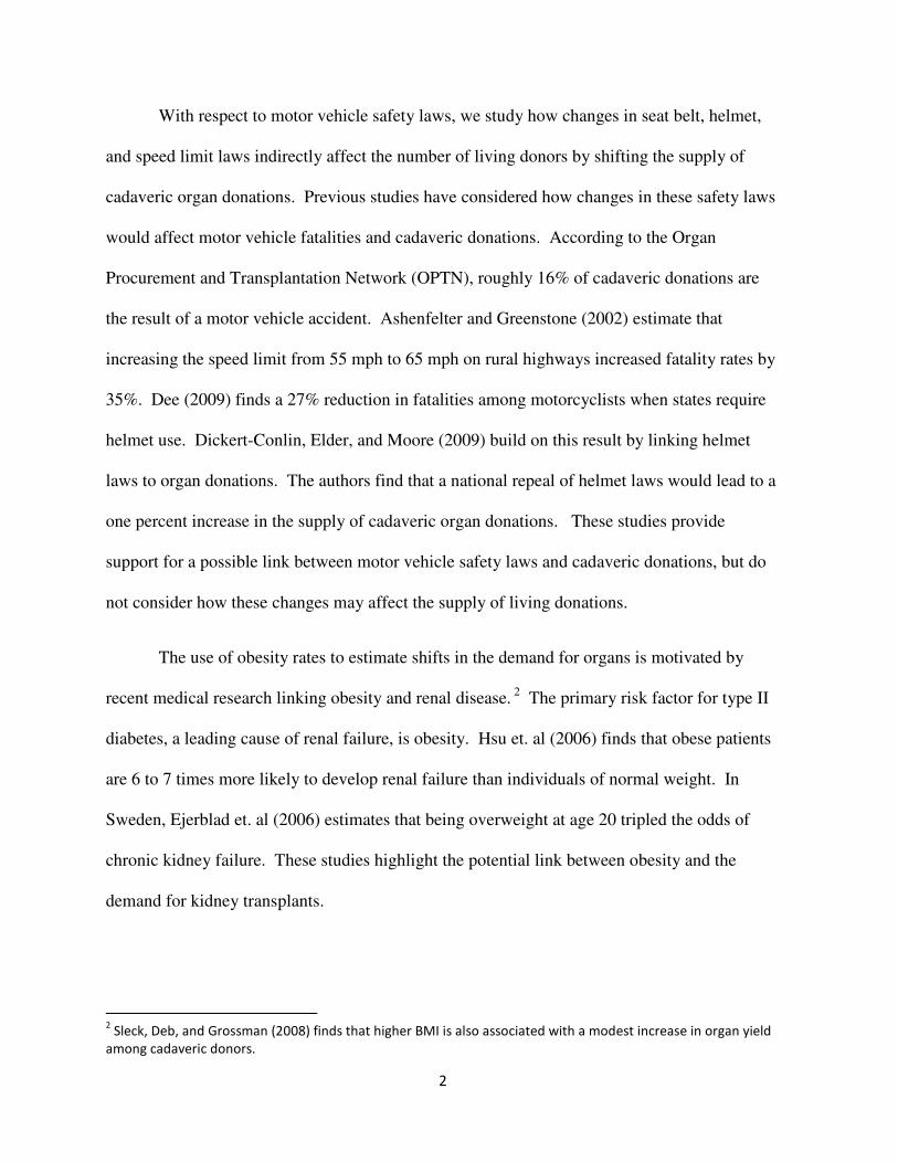
With respect to motor vehicle safety laws, we study how changes in seat belt, helmet,

and speed limit laws indirectly affect the number of living donors by shifting the supply of

cadaveric organ donations. Previous studies have considered how changes in these safety laws

would affect motor vehicle fatalities and cadaveric donations. According to the Organ

Procurement and Transplantation Network (OPTN), roughly 16% of cadaveric donations are

the result of a motor vehicle accident. Ashenfelter and Greenstone (2002) estimate that

increasing the speed limit from 55 mph to 65 mph on rural highways increased fatality rates by

35%. Dee (2009) finds a 27% reduction in fatalities among motorcyclists when states require

helmet use. Dickert-Conlin, Elder, and Moore (2009) build on this result by linking helmet

laws to organ donations. The authors find that a national repeal of helmet laws would lead to a

one percent increase in the supply of cadaveric organ donations. These studies provide

support for a possible link between motor vehicle safety laws and cadaveric donations, but do

not consider how these changes may affect the supply of living donations.

The use of obesity rates to estimate shifts in the demand for organs is motivated by

recent medical research linking obesity and renal disease. 2 The primary risk factor for type II

diabetes, a leading cause of renal failure, is obesity. Hsu et. al (2006) finds that obese patients

are 6 to 7 times more likely to develop renal failure than individuals of normal weight. In

Sweden, Ejerblad et. al (2006) estimates that being overweight at age 20 tripled the odds of

chronic kidney failure. These studies highlight the potential link between obesity and the

demand for kidney transplants.

2 Sleck, Deb, and Grossman (2008) finds that higher BMI is also associated with a modest increase in organ yield

among cadaveric donors.

3

We propose using state-year variation in motor safety laws and obesity rates as

instruments for the supply of cadaveric organs and the demand for organs in a state,

respectively. These estimates are then used to identify substitution patterns between cadaveric

and living donors. We find three important results. First, living donors do respond to changes

in the supply of cadaveric donors. A 1% decrease in the supply of cadaveric donors per

100,000 increases the supply of living donors per 100,000 by .7%. Only helmet laws are found

to have a statistically significant effect on the supply of cadaveric donors. A national adoption

of helmet laws is estimated to decrease cadaveric kidney donations by 6%, but leads to a 4.2%

increase in the number of living donors or a net effect of 1.8% decrease in the supply of organ

donors. Second, the recent rise in obesity rates is estimated to increase living donor rates by

roughly 18%. Lastly, we provide suggestive evidence that increases in disposable income per

capita are associated with an increase in the number of non-biological living donors within a

state.

In the following section, we provide a brief overview concerning changes in motor

vehicle safety laws in the US. Section 3 describes the data gathered from the Organ

Procurement and Transplantation Network (OPTN) as well as changes in state demographics

used to conduct the analysis. Section 4 presents the empirical model and results. Lastly,

Section 5 concludes.

2. A Brief History of Motor Vehicle Safety Laws

Speed Limits

Prior to 1974, speed limits were determined by states and local governments. The Emergency

Highway Energy Conservation Act (EHECA) of 1974 set speed limits to a maximum of 55

4

mph, which was lower than any existing speed limit within the 50 states. In 1987, Congress

modified the EHECA by allowing states to set speed limits not to exceed 65 mph on rural

highways. Of the 50 states, 41 states did increase speed limits on rural highways to 65 mph.3

The nationwide setting of speed limits was motivated by politicians to mitigate the fuel energy

crisis during the 1970’s and 1980’s.

In 1995, Congress eliminated the national speed limit restriction. States are now free to

choose the maximum speed on both rural and urban highways. By 1997, most states had

adopted speed limits of 70 mph or greater on rural highways, but only half set limits above the

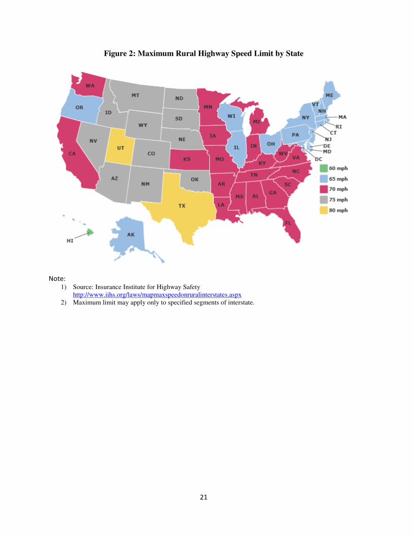
previous national limit of 55 mph on urban highways. As of June 2009, 33 states have

speeding limits in excess of 65 mph on rural highways with the highest speed limit being 80

mph in Texas and Utah. Only 14 states have maintained the national speed limit of 55 mph on

rural highways and the lowest speed limit is found in Hawaii at 50 mph. Figure 2 provides a

summary of current speed limits on rural interstate highways by state.

According to the National Highway Traffic and Safety Administration, speeding is

associated with roughly one-third of all fatal crashes. In 2007, 13,040 people died in speed

related crashes. An increase in travel speed decreases a driver’s reaction time and increases the

force of impact in the event of a crash. Yet, the evidence of speed limits having a significant

effect on fatalities is mixed. Ashenfelter and Greenstone (2002) report that immediately

following the passage of the 1974 Emergency Highway Energy Conservation Act, which

restricts speed limits to 55 mph nationwide, fatalities per mile decreased by 15%. The National

Research Council provides in their 1984 report Highway Statistics evidence that the nationwide

3 Only seven states maintained the national speed limit on urban highways: Connecticut, Maryland,

Massachusetts, New Jersey, New York, Pennsylvania, and Rhode Island. Delaware, the District of Columbia, and

Hawaii did not have highways classified as rural.

5

speed restriction prevented 3,000 to 5,000 traffic fatalities annually. However when the

restriction was lifted on rural highways in 1987, it was thought that fatalities would increase.

Lave (1990) finds the increase in speed limits may have saved 3,113 lives between 1987 and

1988. Further, Moore (1999) finds the 1995 repeal of a nationwide speed limit on urban

highways led to 66,000 fewer road injuries in 1997 than in 1995.

Helmet Laws

In 1967, the federal government encouraged states to adopt universal helmet laws by

making the issue a stipulation to qualify for federal safety programs and highway construction

funds. The universal helmet law requires all riders, regardless of age, to wear a helmet. In the

early 1970’s, most states had adopted a helmet law with the exception of Michigan, which

repealed the law in 1968. In 1976, Congress removed the mandate requiring states to have

helmet laws in order to receive federal highway funds. By 1980, most states had repealed

these or stipulated partial coverage laws, which would only apply to young riders (18 years old

and younger). Currently, all but 3 states (Illinois, Iowa, and New Hampshire) have some form

of helmet law. Since 1997, Arkansas, Florida, Kentucky, Pennsylvania, and Texas have moved

from universal to partial helmet laws. In 2004, Louisiana moved from a partial to a universal

helmet law. Figure 3 summarizes current helmet laws by state. The changes in helmet law

adoption and type between states have created a natural experiment used by researchers to

study the effects of these laws on helmet use, fatalities, and demand [See Dee (2009), Liu et.

al. (2008), and Sass and Zimmerman (2000)].

Seat belt Laws

6

In 1984, New York was the first state to require front seat occupants to wear a seat belt.

Today, mandatory seat belt laws are found in every state with the exception of New

Hampshire.4 In 30 states, the seat belt law is a primary law implying that police officers may

stop a vehicle solely because the occupants are not wearing seat belts. In the remaining states,

where belt laws are considered secondary laws, a police officer must have an alternative reason

to stop a vehicle prior to giving a seat belt citation. Since 1993, 23 states have moved from a

secondary belt law to a primary belt law. The average fine is $32 with five states issuing the

lowest fine of $10 and Texas issuing the highest fine of $200. Cohen and Einav (2001) use

data from 1983 to 1997 for all 50 states and the District of Columbia to estimate the

effectiveness of seat belt laws to reduce fatalities. The authors find that a 10% increase in seat

belt usage decreases automobile fatalities by about 1.35 percent or 500 lives annually.

3. Data

The 1984 National Organ Transplant Act (NOTA) established the Organ Procurement

Transplantation Network (OPTN) a network of 57 Organ Procurement Organizations (OPO)

located in 37 states and the District of Columbia. These OPO’s are given monopoly rights to

receive and transplant organs within a designated service area. The OPTN has maintained

organ donation data collected from each OPO since 1988.5 This paper uses kidney donation

counts from 1988 – 2008 with respect to cadaveric donors and living donors. Living donors are

disaggregated into biological and non-biological donors.

As illustrated in Figure 1, the number of living donors has increased dramatically over

the last twenty years. Perhaps more interestingly, the percent of living donors who are not

4 These laws cover front-seat occupants only, although belt laws in 21 states and the District of Columbia cover all

rear seat occupants as well. See Figure 4 for current belt laws by state. 5 The OPTN publicly provides these data on their website www.OPTN.org

7

related to the donee has also increased from roughly 7% in 1988 to 40% in 2008. One reason

for this increase is a change in the surgical procedure used to harvest the kidney. Prior to the

introduction of laparoscopic surgery, a 4 to 7 inch incision was needed to retrieve the kidney,

which would significantly increase the pain and recovery time associated with the procedure.

According to Schweitzer et. al. (2000), the use of laparoscopic surgery has decreased hospital

recovery time from four and a half days to three days and has allowed donors to return to work

27 days faster. Clearly, this medical advancement decreases the non-pecuniary cost of

donating an organ for a living donor, but costs are also decreased to the donee. Although

NOTA stipulates it is unlawful to provide financial compensation to the donor, the ordinance

does allow for payment to cover expenses directly incurred by the organ donor for the purposes

of the donation, like travel costs and lost wages.6 These non-medical cost are not covered by

insurance. Instead, these costs are paid out of pocket. By reducing time away from work,

compensation associated with lost wages is also decreased. This incentive can potentially

establish a link between non-biological donors and disposable income.

Although, OPO’s may serve several surrounding states, we follow Dickert-Conlin,

Elder, and Moore (2009) in aggregating up to the state in which the OPO’s reside. Each year

we observe 37 states and the District of Columbia for a total of 798 site-year observations.7

For each state, we collect information on helmet laws, seat belt laws, and speed limits from the

Insurance Institute of Highway Safety. State population data is gathered from the US Census.

The U.S. Bureau of Economic Analysis provides data on State Disposable Income Per Capita.

6 Medical expenses for the donor are covered by the donee’s insurance. About 80% of the transplant cost is

covered by Medicare and the remaining 20% is covered by private insurance. 7 There are no centers in Delaware, Idaho, Maine, Montana, New Hampshire, North Dakota, South Dakota,

Vermont, and Wyoming.

8

The data are inflation-adjusted to the base year of 2000. Lastly, statewide obesity rates are

provided by the Centers for Disease Control (CDC) and Prevention.8

Descriptive statistics for each of the variables are found in Table 1. Over the entire

sample, cadaveric donors, on average, outpaced living donors by a ratio of 5 to 4, but the

number of living donors exceeded the number of cadaveric donors from 2000-2005. Within

living donors, 73% are from biological donors, 57% of living donors are female, 45% are

between the ages of 35-49, and 36% are between the ages of 18-34. Among cadaveric donors,

60% are male, 10% are 11-17 years old, 30% are 18-34 years old, 26% are between 35-50

years old, and 28% are greater than 50 years old.

Obesity rates in the U.S. have risen steadily since the 1990’s. By definition, an obese

individual has a Body Mass Index (BMI) of 30 or greater.9 The CDC reports statewide obesity

rates as the percentage of 30 year olds in the state with a BMI greater than or equal to 30.

According to the CDC:

10 states had a prevalence of obesity less than 10% and no states had prevalence equal to or greater than 15% in 1990. By 1998 no state had a prevalence of obesity less than 10%. In 2007, only one state (Colorado) had a prevalence of obesity less than 20%. Thirty states reported a prevalence equal to or greater than 25% and three states (Alabama, Mississippi and Tennessee) had a prevalence of obesity equal to or greater than 30%.

These increases in obesity rates appear to coincide with increases in the number of living

donors and the size of the organ donor waiting list. We find that 81% of the states in our

sample report obesity rates between 10%-24%.

8 US Obesity Trends by State from 1985 – 2008 http://www.cdc.gov/obesity/data/trends.html. 21 observations

are lost due to missing obesity data for Arkansas, Colorado, the District of Columbia, Maryland, New Jersey, and

Pennsylvania in a few years. 9 Body Mass Index (BMI) is calculated as a person’s weight in kilograms divided by the square of his/her height in

meters. BMI is not a perfect measure for obesity as it fails to account for muscular mass versus fat.

9

Referring back to Table 1, we do observe large variations in helmet laws and seat belt

laws between the states. This is reflected in the large standard deviation for these four

variables and is expected due to the many adoptions, repeals, and modifications these laws

experienced during the period of our sample. On the other hand, speed limits display little

variation as 56% of the states report rural speed limits equal to 65 mph and 57% report urban

speed limits of 55 mph or less. In addition, much of the changes in speed limits occurred

shortly after the 1987 modification to the Emergency Highway Energy Conservation Act and

the 1995 repeal.10

4. Model and Results

Consider the following conceptual model based on living donors being altruistic. A living

donor’s utility function takes the form of

�1� ���, �, , � = max�� + � ∗ ∗ ���������� , � − + � ∗ �����������

where H represents the donor’s Health level, c is cost to health for donating an organ, p is the

probability the organ recipient receives an organ from a cadaveric donor, � is the level of

altruism the donor has for the organ recipient. According to United Network of Organ Sharing

organization, patients receiving a kidney from a living donor (LD) rather than a cadaveric

donor (CD) have higher survival rates. For this reason, we assume an organ recipient’s utility

is higher when receiving an organ from a living donor, U(LD)>U(CD). In relative utility, the

potential donor chooses not to donate if > ������������ − ����������� or the cost of

donation is greater than the relative expected benefit of supplying an organ from a living

donor. As previously discussed, costs faced by the donor include pain associated with the

procedure, lost wages due to time away from work for the procedure, and potentially can

10

These events present a problem during estimation in that the use of year fixed effects may confound the

effect of speed limit changes.

10

include lower lifetime income due to a lower lifetime level of health. As costs tend to

decrease, due to advancements in medicine, the supply of living donors should increase, ceteris

paribus.

Altruism plays an important role in this model as well. For our purposes, altruism is

captured by allowing the donor’s utility to be dependent upon the donee’s utility. Further, the

more familiar a donor is with the done the larger � becomes in the donor’s utility function.

Altruism allows there to be a positive supply of organs at a price of zero.11 The probability of

receiving a cadaveric organ, p, is a function of the size of the waiting list and the level of

altruism in society associated with donating organs at death. As the waiting list increases, p

decreases, thereby encouraging more living donations. If the level of altruism among

cadaveric donors rises in society, then p increases and causes living donor rates to marginally

decrease. On the other hand, if altruism rises among living donors, then the level of donations

from living donors rises. In an effort to increase altruism among potential living donors,

websites such as livingdonors.org and matchingdonors.com provide information pertaining to

patients in need of an organ. These sites can increase living donor rates by personalizing organ

matches; thereby increasing altruism on the part of the donor, � ����� � .

The duality of altruism in society plays an important role when estimating the

substitution effect between living and cadaveric donors. If certain states are more altruistic

than others, then one may observe both higher rates of cadaveric and living donations in those

high altruistic states. The level of altruism in a state is an unobserved variable, but we need to

control for altruism in order to obtain unbiased estimates on the effect of cadaveric donors on

11

See Epstein (2008) for a discussion on the effects of altruism on organ supply.

11

the supply of living donors. We use an instrumental variables approach to control for the

econometric endogeneity problem caused by unobserved altruism.

Our estimation strategy uses organ demand shifters (changes in obesity rates) and

supply shifters (seat belt laws, helmet laws, and speed limits) as instruments to identify

potential substitution patterns between cadaveric and living donors. These instruments are

independent of state specific levels and changes in altruism among organ donors. Using a two

staged least squares approach, we first estimate the effect of traffic safety laws on the supply of

cadaveric organs, then estimate living donors as a function of obesity rates and predicted

cadaveric donors.

In the first stage, we estimate the following model:

�2� ��#$ = %�&�'#$� + (#$) + �#$

where CDst represents cadaveric kidney donations per 100,000, s indexes state, t indexes year,

&�'#$ is a matrix of dummy variables capturing changes in traffic safety laws (full and partial

helmet laws, primary and secondary seat belt laws, rural highway speed limits, and urban

highway speed limits), and (#$ is a matrix containing state disposable per capita income and

state population.12

The unobserved error est captures all unobserved changes within a state and overtime

associated with cadaveric donations. These unobserved measures may include variation in the

causes of hospital deaths, changes in medical technology, and differences in altruism. Two

12

Beard, Kaserman, and Saba (2006) and Dickert-Conlin, Elder, and Moore (2009) use a similar equation to

capture cadaveric donations.

12

specifications of the error term are proposed to control for these unobserved changes:

(3) �#$ = *# + +$ + ,#$ �#$ = *# + -#.�/� + ,#$

where *# is a state fixed effect, +$ is a year fixed effect, -# is a state specific time trend, and ,#$

is an idiosyncratic state-year shock. The first specification of the error term is commonly used

to exploit the panel nature of the data. The second specification treats changes in time as a

linear function. We find this specification useful because the instruments we use are primarily

dummy variables that change depending on year and state. The year fixed effect may

confound some of these effects.

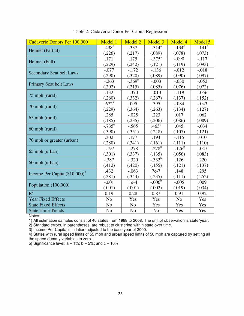
Table 2 contains estimates of % and ) under different specifications of the error term.

All specifications are weighted by state population and include standard errors, which are

robust to clustering within state over time. Each column represents a progression in controls

with respect to the error term. Column (1) indicates that helmet laws (both full and partial)

would lead to an increase in cadaveric donors (21% increase with partial helmet laws and 8%

increase with full helmet laws), seat belt laws are not found to affect donor rates in a

statistically significant manner, and rural speed limits are found to decrease donations at 60

mph by 36%, but increase them at 70 mph by 33%. Yet, as shown in Columns (4) and (5),

these correlations tend to be spurious when state and time fixed effects are used. Only partial

helmet laws are found to be statistically significant at the 5% level. Partial helmet laws

decrease cadaveric kidney donations -.14 per 100,000 population or -6.8%. These estimates

are on par with Dickert-Conlin, Elder, and Moore (2009) who find a 10% decrease using all

organ types.

13

In the second stage, we use predicted levels of cadaveric kidney donors along with

changes in obesity rates to capture substitution patterns between living and cadaveric organ

donors. The living donor equation is specified as follows:

�4� ��#$ = %1��2 #$3 + 456� �.7#$ + (#$) + �#$

where LD measures living kidney donors per 100,000 population, ��2 #$ are predicted cadaveric

donors per 100,000 population, Obesity is a matrix of dummy variables separating each state s

in year t into the following categories as a percentage of the population who is obese: 10-14%,

15-19%, 20-24%, and 25% or greater. The null set contains states with obesity rates less than

10%. The potential for endogeneity of cadaveric organs stems from unobserved altruism.

Although individuals incur a smaller cost when donating organs at the time of their death than

when they are alive, there must still be some level of altruism present for organs to be supplied

at a price of zero. Therefore, advertisement campaigns and websites that encourage organ

donations may increase levels of altruism to both living and cadaveric donors. Failing to

control for altruism may lead researchers to conclude that the number of living donors and

cadaveric donors are positively correlated. We propose using traffic safety laws as instruments

for the supply of cadaveric donors. Many of these laws are initially adopted by states because

the federal government tied federal highway maintenance/construction funds to these laws.

Therefore, these laws were neither adopted to affect altruism levels in the state, nor to

manipulate the supply of cadaveric/living organ donors.

Table 3 illustrates how the supply of cadaveric organ donors affects the level of living

donors per capita. All specifications in this table use state fixed effects and robust standard

errors that are clustered by state over time. Note, the effect of cadaveric donors on the supply

of living donors is indistinguishable from zero in the first two columns when ordinary least

14

squares (OLS) is used.13 In column 3, the use of state specific time trends increases the

magnitude of the coefficient to -.249 or a decrease of 15% in living donors for 1 additional

cadaveric donor per 100,000. Using instrumental variables, this coefficient increases in

magnitude ranging from (-.375,-.614). Our most preferred specification (IV3) utilizes state

specific time trends and finds that 1 additional cadaveric donor per 100,000 is found to

decrease the number of living donors per 100,000 by 37%. This result is statistically

significant at the 1% level. Using a back of the envelope calculation, the effect of helmet laws

on the supply of living donors is inferred to increase living donor rates by 4.2%.14

In addition to this substitution effect, we find mixed results with respect to obesity

rates. In all of the specifications (except for IV2) the obesity indicators are found to increase

the level of living donors. The largest contributors are states with obesity rates between 15-

19% and 20-24%. The average effect for these two groups across the models is .256 living

donors per 100,000 (an increase of 16%) and .285 living donors per 100,000 (an increase of

17%). These obesity indicator variables capture both current and future demand for organs.

As the demand for organs rises, the probability of receiving a cadaveric organ decreases

because the waiting list becomes longer; thereby increasing the net benefit to a living donor.

As previously mentioned, the use of year fixed effects greatly diminishes the effect of obesity

rates on living donors. In OLS2 and IV2, the coefficients of the obesity indicator variables

decrease in magnitude and are statistically indistinguishable from zero. When state specific

13

Both with no fixed effects or only year fixed effects, we find a positive point estimate on cadaveric donors per

capita when estimated using OLS. 14

Helmet laws decrease kidney cadaveric donors by 6%. Living donors per 100,000 decreases by .614 for one

additional cadaveric donor per 100,000; therefore, helmet laws increase living donor rates by .042=(.06)(.614)

15

time trends are used, obesity rates between 15 – 24% are found to be statistically significant at

the 1% level and point estimates for all the obesity variables are positive.15

Lastly, we turn our attention to non-biological living donors. The use of laparoscopic

surgery to remove kidneys has greatly reduced pain and recovery time for living donors. In

addition to the reduction of these non-pecuniary costs, this procedure has allowed donors to

return to work faster leading to fewer lost wages. Although not covered by public or private

insurance, NOTA does allow donors to be compensated for travel, lost wages, child care, and

other expenses that are directly related to the transplant procedure.16 Therefore, a link between

disposable income and non-biological kidney donors potentially exits.

The living donor variable in equation (4) is disaggregated into biological and non-

biological donors. Equation (4) is re-estimated under these two subsamples and the estimates

are found in Table 4. For brevity we focus our discussion on disposable state income per

capita and state population.17 The dependent variable is estimated both in levels and per capita

(100,000 population). Disposable income per capita is found to be statistically significant only

with respect to non-biological donors. An increase of $10,000 in state income per capita

increases the number of non-biological donors by 30.8 (.117 per capita), which is equivalent to

an increase in the living donor rate by 7%. Disposable income per capita is estimated to have a

15

We also consider using average charitable contribution levels from IRS tax returns between 1997-2007 as a

proxy for altruism. An increase in charitable contributions is found to have a positive and statistically significant

effect on living donor rates, but contributions levels do not affect the IV point estimates on the effect of

cadaveric donor rates on living donor rates. These results are available from the authors. 16

We do consider the role of health insurance on the supply of living donors. We collected data from the March

CPS and constructed variables capturing the percentage of individuals with no health insurance, private

insurance, and government insurance. These variables are not found to have a statistically distinguishable affect

on living donor rates at conventional levels. These estimates are available from the authors upon request. 17

Interested readers can obtain the other estimated coefficients from the authors, but the qualitative results do

not vary greatly from those found using living donors as the dependent variable.

16

positive effect in both the biological donor equation and the living donor equation, but neither

coefficient is distinguishable from zero at conventional significance levels.

5. Conclusion

The discussion on the organ shortage is full of suggestions on how to alleviate the

problem, but little empirical evidence exists discussing the motives and incentives surrounding

living donors. In this paper, we consider how living donors react to changes in the supply of

cadaveric donors and the looming obesity epidemic. We propose an instrumental variables

model to control for unobserved variation in altruism between states, which may potentially

cause a positive correlation between living and cadaveric donors within a state. Utilizing

variation in traffic safety laws as instruments for the supply of cadaveric donors, we estimate

that one additional cadaveric kidney donor per 100,000 decreases living donors by .614 per

100,000 or 37%. Further, a nationwide repeal on helmet laws would lead to a net increase in

kidney donations of 1.8%. In addition to these results, we find the rise in obesity within the

United States has contributed to the increase in living donor rates by as much as 17% and state

disposable income per capita is positively correlated with the rate of non-biological living

donors, but not biological living donors.

Although further research is necessary, understanding the trade-offs faced by living

donors is important to allow for more informed policy choices. Less than 1 percent of hospital

deaths are suitable for organ transplant.18 The organ shortage will not be resolved through

cadaveric donations alone, but rather in conjunction with living donations. Currently,

compensation for organs is considered unlawful, but a potential alternative may come in the

18

A majority of hospital deaths leading to organ donation are associated with brain dead patients, but their

currently are developments to increase the number of donations from patients who die of cardiac arrest. See

http://www.organtransplants.org/understanding/death/

17

form of a tax incentive. The Organ Donation and Recovery Improvement Act (H.R. 3926),

which was signed into law on April 5, 2004, has a provision allowing states to offer tax

deductions for organ donors. As of this paper, 12 states have adopted tax deductions of up to

$10,000, and another 18 are considering similar ordinances.19

19

Arkansas, Georgia, Iowa, Louisiana, Minnesota, Mississippi, New Mexico, New York, North Dakota, Ohio,

Oklahoma, Utah, and Wisconsin have adopted tax deductions for organ donations. Hawaii, Idaho,

Massachusetts, Missouri, Texas, and Virginia allow organ donors to receive paid leave of absence. For more

information see http://www.transplantliving.org/livingdonation/financialaspects/

18

References:

Abadie, A. and S. Gay “The Impact of presumed consent legislation on cadaveric organ donation: A cross-country study,” Journal of Health Economics, 25 (2006) 599-620 Ashenfelter, Orley and Micahel Greenstone. "Using Mandated Speed Limits To Measure The Value Of A Statistical Life," Journal of Political Economy, 2004, v112(2,Part2), S226-S267. Beard, T. R., Kaserman, D. L. and R. P. Saba, "Inefficiency in Cadaveric Organ Procurement," Southern Economic Journal, 2006 vol. 73(1), pages 13-26, July. Becker, G. and J. Elias “Introducing Incentives in the Market for Live and Cadaveric Organ Donations” Journal of Economic Perspectives Vol. 21, Number 3 (Summer) 2007 pg. 3-24 Byrne, M. and P. Thompson, “A positive analysis of financial incentives for cadaveric organ donation” Journal of Health Economics 20 (2001) 69–83 Center for Disease Control and Prevention, “Obesity Trends Among US Adults: 1985-2008” http://www.cdc.gov/obesity/downloads/obesity_trends_2008.pdf Cohen, A. and L. Einav “The Effects of Mandatory Seat Belt Laws on Driving Behavior and Traffic Fatalities” Review of Economics and Statistics, 2003 Vol. 85:4, 828-843 Dee, T., “Motorcycle helmets and traffic safety” Journal of Health Economics 28 (2009) 398–412 Dickert-Conlin, S., Elder, T., and B. Moore, “Donorcycles: Do Motorcycle Helmet Laws Contribute to the Shortage of Organ Donors?” Michigan State University June 10, 2009 mimeo. Ejerblad, E., Fored, C. M., Lindblad, P., Fryzek, J., McLaughlin, J. K. and O. Nyre´n “Obesity and Risk for Chronic Renal Failure” J Am Soc Nephrol 17: 1695–1702, 2006. Epstein, R. “The Human and Economic Dimensions of Altruism: The Case of Organ Transplantation” The Journal of Legal Studies, Vol. 37, No. 2. (1 June 2008), pp. 459-501. Howard, D. H. “Producing Organs” Journal of Economic Perspectives Vol. 21, Number 3 (Summer) 2007 pg. 25–36 Howard, D.H. “Why do transplant surgeons turn down organs? A model of the accept/reject decision” Journal of Health Economics 21 (2002) 957–969 Hsu, C., C. E. McCulloch, C. Iribarren, J. Darbinian and A. S. Go, “Body Mass Index and Risk for End-Stage Renal Disease” Ann Intern Med 2006; 21-28.

19

Lave, C. and P. Elias “Did the 65 MPH Speed Limit Save Lives?” Accident Analysis and Prevention Vol. 26, No. 1 (1994), pp. 49-62 Liu BC, Ivers R, Norton R, Boufous S, Blows S, Lo SK. Helmets for preventing injury in motorcycle riders. Cochrane Database of Systematic Reviews 2008, Issue 1. Art. No.: CD004333. DOI: 10.1002/14651858.CD004333.pub3. Moore, S. “Speed Doesn’t Kill: The Repeal of the 55-MPH Speed Limit” Policy Analysis No. 346 May 31, 1999 Roth, A. “Repugnance as a Constraint on Markets” Journal of Economic Perspectives Vol. 21, Number 3 (Summer 2007) pg 37–58 Sass, T.R. and P.R. Zimmerman, “Motorcycle helmet laws and motorcyclist fatalities.” Journal of Regulatory Economics 18 (2000) 195-215. Schweitzer, Eugene J., MD, Jessica Wilson, BSN, Stephen Jacobs, MD, Carol H. Machan, BA, Benjamin Philosophe, MD, PhD, Alan Farney, MD, PhD, John Colonna, MD, Bruce E. Jarrell, MD, and Stephen T. Bartlett, MD “Increased Rates of Donation With Laparoscopic Donor Nephrectomy” ANNALS OF SURGERY Vol. 232, No. 3, 392–400 Selck, F. W., Debb, P. and E. B. Grossman, “Deceased Organ Donor Characteristics and Clinical Interventions Associated with Organ Yield” American Journal of Transplantation 2008; 8: 965–974

20

0

0.1

0.2

0.3

0.4

0.5

0.6

0.7

0.8

0.9

1

0

1

2

3

4

5

6

7

8

1988 1992 1996 2000 2004 2008

Do

no

rs (

1,0

00

)Figure 1: Trends in Donor Types and Rates

Living Donor Deceased Donor Ratio of Biological/Living Donor

Bio

log

ica

l/Li

vin

g D

on

ors

21

Figure 2: Maximum Rural Highway Speed Limit by State

Note: 1) Source: Insurance Institute for Highway Safety

http://www.iihs.org/laws/mapmaxspeedonruralinterstates.aspx 2) Maximum limit may apply only to specified segments of interstate.

22

Figure 3: Motorcycle Helmet Laws by State

Note:

1) Source: Insurance Institute for Highway Safety http://www.iihs.org/laws/HelmetUseCurrent.aspx#IA 2) Universal coverage requires that all riders wear helmets 3) Partial coverage states that riders under an age determined by the state are required to wear helmets

23

Figure 4: Seat belt Laws by State

Note:

1) Source: Insurance Institute for Highway Safety http://www.iihs.org/laws/HelmetUseCurrent.aspx#IA 2) Primary enforcement stipulates that a vehicle may be stopped solely for this offense. 3) Secondary enforcement stipulates that an additional fine may be assessed after stopping the vehicle for a

different violations granted that the passengers are not wearing their seat belts

24

Table 1: Descriptive Statistics

Variables Mean STD Min Max

Living Donors 109.95 120.85 0.00 743.00

Living Donors per 100,000 1.64 1.70 0.00 24.09

Cadaveric Donors 138.40 128.47 7.00 838.00

Cadaveric Donors per 100,000 2.05 1.22 0.44 18.96

Biological Donors 79.81 81.36 0.00 500.00

Biological Donors per 100,000 1.18 0.85 0.00 9.57

Less than 10% Obese 0.06 0.24 0.00 1.00

10% - 14% Obese 0.27 0.44 0.00 1.00

15% - 19% Obese 0.28 0.44 0.00 1.00

20% - 24% Obese 0.26 0.44 0.00 1.00

25% � Obese 0.13 0.33 0.00 1.00

Secondary Seat belt Laws 0.56 0.22 0.00 1.00

Primary Seat belt Laws 0.39 0.49 0.00 1.00

Helmet Law (Partial) 0.41 0.49 0.00 1.00

Helmet Law (Full) 0.51 0.50 0.00 1.00

75 mph (rural) 0.11 0.32 0.00 1.00

70 mph (rural) 0.24 0.43 0.00 1.00

65 mph (rural) 0.56 0.50 0.00 1.00

60 mph (rural) 0.04 0.19 0.00 1.00

55 mph or less (rural) 0.05 0.21 0.00 1.00

70 mph or greater (urban) 0.13 0.33 0.00 1.00

65 mph (urban) 0.26 0.44 0.00 1.00

60 mph (urban) 0.05 0.21 0.00 1.00

55 mph or less (urban) 0.57 0.50 0.00 1.00

State Population Per 100,000 68.01 62.85 5.85 367.57

State Disposable Income Per Capita ($10,000) 2.68 0.53 1.57 5.20

25

Table 2: Cadaveric Donor Per Capita Regression

Cadaveric Donors Per 100,000 Model 1 Model 2 Model 3 Model 4 Model 5

Helmet (Partial) .438c

(.226) .337

(.217) -.314a

(.089) -.134c

(.078) -.141c

(.073)

Helmet (Full) .171

(.229) .175

(.242) -.375a

(.121) -.090 (.119)

-.117 (.093)

Secondary Seat belt Laws -.077 (.290)

-.172

(.320) -.136 (.089)

-.012 (.090)

-.018 (.097)

Primary Seat belt Laws -.263 (.202)

-.369c

(.215) -.003 (.085)

-.030 (.076)

-.052 (.072)

75 mph (rural) .132

(.260) -.370 (.332)

-.013 (.267)

-.119 (.137)

-.056 (.152)

70 mph (rural) .672a

(.229) .095

(.364) .395

(.263) -.084 (.134)

-.043 (.127)

65 mph (rural) .285

(.185) -.025 (.235)

.223 (.206)

.017 (.086)

.062 (.089)

60 mph (rural) -.735c

(.390) -.565 (.351)

.463c

(.248) .045

(.107) -.034 (.121)

70 mph or greater (urban) .302

(.280) .177

(.341) .194

(.161) -.115 (.111)

.010 (.110)

65 mph (urban) -.197 (.301)

-.278 (.337)

-.278b

(.135) -.126b

(.056) -.047 (.083)

60 mph (urban) -.387 (.412)

-.320 (.420)

-.332b

(.155) .126

(.121) .220

(.137)

Income Per Capita ($10,000)3 .432 (.281)

-.063 (.344)

7e-7 (.235)

.148 (.111)

.295 (.252)

Population (100,000) -.001 (.001)

1e-4 (.001)

-.006b

(.002) -.005 (.019)

.009 (.034)

R2 0.19 0.28 0.87 0.91 0.92

Year Fixed Effects No Yes Yes No Yes

State Fixed Effects No No Yes Yes Yes

State Time Trends No No No Yes Yes Notes: 1) All estimation samples consist of 40 states from 1988 to 2008. The unit of observation is state*year. 2) Standard errors, in parentheses, are robust to clustering within state over time. 3) Income Per Capita is inflation-adjusted to the base year of 2000. 4) States with rural speed limits of 55 mph and urban speed limits of 50 mph are captured by setting all the speed dummy variables to zero. 5) Significance level: a = 1%; b = 5%; and c = 10%

26

Table 3: Living Donor Per Capita Regression

Living Donors Per 100,000 OLS 1 OLS 2 OLS 3 IV1 IV2 IV3

Cadaveric Donors Per 100,000

-.078 (.096)

-.188c

(.111) -.249a

(.087) -.375 (.316)

-.389 (.308)

-.614b

(.299)

10%-14% Obese .234a

(.096) .072

(.093) .096

(.072) .239a

(.103) .024

(.083) .071

(.066)

15%-19% Obese .471a

(.128) .044

(.124) .253a

(.086) .521a

(.155) -.018 (.097)

.241a

(.083)

20%-24% Obese .513a

(.196) -.056 (.184)

.312a

(.120) .724a

(.249) -.052 (.072)

.295a

(.122)

25% � Obese .193

(.288) -.277 (.242)

.044 (.170)

.558 (.397)

-.054 (.147)

.103 (.178)

Income Per Capita ($10,000)

1.62a

(.320) 1.34a

(.566) .186

(.217) 1.68a (.283)

1.35a

(.547) .191

(.209)

Population (100,000) -.013b

(.006) -.017a

(.005) .031

(.036) -.015a

(.005) -.018a

(.005) .030

(.036)

R2 0.84 0.87 0.92 0.84 0.87 0.92

Year Fixed Effects No Yes No No Yes No

State Fixed Effects Yes Yes Yes Yes Yes Yes

State Time Trends No No Yes No No Yes Notes: 1) All estimation samples consist of 40 states from 1988 to 2008. The unit of observation is state*year. 2) Standard errors, in parentheses, are robust to clustering within state over time. 3) States with obesity rates less than 10% are captured by the constant 4) Significance level: a = 1%; b = 5%; and c = 10%

27

Table 4: Biological versus Non-Biological Donors

LEVELS Biological Donors Non-Biological Donors All Living

Donors

Income Per Capita ($10,000)

-24.5 (21.7)

30.6a

(11.7) 6.18

(22.8)

Population (100,000) 9.42

(5.87) 3.27

(3.39) 12.7c

(7.57)

R2 0.97 0.97 0.98

PER CAPITA Biological Donors Non-Biological Donors All Living

Donors

Income Per Capita ($10,000)

.111 (.177)

.177c

(.092) .289

(.219)

Population (100,000) .018

(.019) -.008 (.015)

.010 (.030)

R2 0.90 0.95 0.94 Notes: 1) All estimation samples consist of 40 states from 1988 to 2008. The unit of observation is state*year. All models include year and state fixed effects with state specific time trends. 2) Controls include indicator variables accounting for changes in obesity, seat belt laws, helmet laws, and speed limit laws 3) Standard errors, in parentheses, are robust to clustering within state over time. 4) Significance level: a = 1%; b = 5%; and c = 10%