The effect of wastewater components on the fouling … · The effect of wastewater components on the fouling of ... The effect of wastewater components on the fouling of ... 2.4.3

Loughborough UniversityInstitutional Repository

The effect of wastewatercomponents on the fouling of

ceramic membranes

This item was submitted to Loughborough University's Institutional Repositoryby the/an author.

Additional Information:

• A Doctoral Thesis. Submitted in partial fulfillment of the requirementsfor the award of Doctor of Philosophy of Loughborough University.

Metadata Record: https://dspace.lboro.ac.uk/2134/6457

Publisher: c© Radhi Alazmi

Please cite the published version.

https://dspace.lboro.ac.uk/2134/6457

This item was submitted to Loughborough’s Institutional Repository (https://dspace.lboro.ac.uk/) by the author and is made available under the

following Creative Commons Licence conditions.

For the full text of this licence, please go to: http://creativecommons.org/licenses/by-nc-nd/2.5/

i

Thesis Access Form Copy No…………...…………….Location……………… Author……RADHI ALAZMI…………………………………..……. Title…The effect of wastewater components on the fouling of ceramic membrane. Status of access OPEN / RESTRICTED / CONFIDENTIAL Moratorium Period:…………………………………years, ending…………../…………200………………………. Conditions of access approved by (CAPITALS):……V. NASSEHI..… Supervisor (Signature)……………………...…………………………… Department of……Chemical Engineering……..……………………….. Author's Declaration: I agree the following conditions:

Open access work shall be made available (in the University and externally) and reproduced as necessary at the discretion of the University Librarian or Head of Department. It may also be digitised by the British Library and made freely available on the Internet to registered users of the EThOS service subject to the EThOS supply agreements.

The statement itself shall apply to ALL copies including electronic copies: This copy has been supplied on the understanding that it is copyright material and that no quotation from the thesis may be published without proper acknowledgement. Restricted/confidential work: All access and any photocopying shall be strictly subject to written permission from the University Head of Department and any external sponsor, if any. Author's signature………………………….Date………………………...…………...……...

users declaration: for signature during any Moratorium period (Not Open work): I undertake to uphold the above conditions:

Date Name (CAPITALS) Signature Address

ii

The effect of wastewater components

on the fouling of ceramic membranes

By

Radhi Alazmi

Doctoral Thesis

Submitted in partial fulfilment of the requirements for the

award of Doctor of Philosophy of Loughborough University

© by Radhi Alazmi (2010)

iii

Certificate of Originality This is to certify that I am responsible for the work submitted in this thesis, that the

original work is my own except as specified in acknowledgments or in footnotes, and

that neither the thesis nor the original work contained therein has been submitted to

this or any other institution for a higher degree.

Author's signature ……………………………………………………………… Date ……………………………..

iv

Acknowledgements

I would like to begin with thanking almighty Allah (God) for all his blessing and

grace upon me in this life.

I wish to thank my family especially my wife for all the patient and

encouragement they showed during the years I spent doing this work.

I wish to thank my supervisors Professor Richard Wakeman and Professor

Vahid Nassehi for their guidance and advice which helped me to identify the

crucial and the most important areas in membrane filtration to concentrate my

research in.

I would like to thank Chris Manning the Experimental Officer in the Chemical

Engineering Department at Loughborough University for his help with the

experimental apparatus design and maintenance. I also would like to thank

the Laboratory supervisor Sean Creedon and Dave Smith for all their training

and help with the laboratory equipments.

v

ABSTRACT

In this work, the effect of wastewater feed composition on the membrane

fouling rate of 5 and 20 kD ultrafiltration ceramic membranes was investigated

using statistical analysis of the experimental results (two way factorial design),

with particular regard to the protein (meat extract and peptone), sodium

alginate and calcium chloride components. A mathematical model was used

to determine the major membrane blocking mechanisms and the effect of

different feed components concentration on the blocking mechanisms.

Polysaccharides are the major fouling compounds in extracellular polymeric

substance (EPS), while protein compounds are an important part of EPS

membrane fouling, their effect increases in the presence of polysaccharides.

Sodium alginate calcium solutions fouled the membrane more severely,

causing twice the increase of resistance (on average) than did meat extract

calcium solutions. This study showed that irreversible fouling was the major

fouling type in alginate calcium filtration experiments, while less of the fouling

in the meat extract calcium filtration experiments was irreversible.

The effect of changing the artificial wastewater components concentration on

the fitting accuracy of the blocking models for the 20 kD pore size membrane

was almost the opposite of the 5 kD pore size membrane. Increasing the

calcium concentration increased the predication accuracy of the intermediate

and complete blocking models, while the increase in alginate concentration

reduced the cake filtration model prediction accuracy.

After each experiment, the membrane was cleaned using different cleaning

chemical concentrations. The best cleaning was achieved with increasing

sodium hydroxide concentration in the cleaning solution. In general higher

cleaning temperature and increasing cleaning time improved the membrane

recovery, nevertheless; the effect was not as noticeable as the effect of

increasing sodium hydroxide concentration.

vi

Table of Contents

ACKNOWLEDGEMENTS I

ABSTRACT V

TABLE OF CONTENTS VI

LIST OF TABLES XI

LIST OF FIGURES XIII

1.0 INTRODUCTION 1

1.1 Global Water Shortage 1

1.2 Water treatment 1

1.3 Membrane Wastewater treatment 2

1.4 Research Aims and Objectives 3

2.0 LITERATURE REVIEW 4

2.1 Wastewater Technology 4 2.1.1 Conventional activated sludge process 4

2.2 Membrane technology 5 2.2.1 Membrane bioreactor 6

2.2.2 Membrane structure 7

2.2.3 Membrane materials 9

2.3 Microfiltration and ultrafiltration 10 2.3.1 Microfiltration 11

2.3.2 Ultrafiltration 12

2.4 Theories of bioflocculation mechanisms 13 2.4.1 Effect of particle size and particle size distribution 14

2.4.2 Effect of crossflow velocity on microfiltration flux 16

2.4.3 Effect of yeast cells on microfiltration flux 18

2.4.4 Biomass effect on membrane fouling 19

vii

2.4.5 Role of Extracellular Polymeric Substances (EPS) in membrane fouling 20

2.4.6 Role of cations in membrane fouling 22

2.4.7 Morphology effects on membrane fouling 23

2.4.8 Intermittent effects on membrane fouling 25

2.4.9 Reversible and irreversible fouling 25

2.5 Membrane cleaning methods 26 2.5.1 Physical cleaning 26

2.5.1.1 Forward flush 26

2.5.1.2 Backward flush 26

2.5.2 Chemical cleaning processes 29

2.5.3 Biofilm removal 31

2.6 Crossflow membrane filtration modelling 31

2.7 Dead end blocking models 31 2.7.1 Combined blocking mechanisms models 33

2.7.2 Concentration Polarisation Theory 35

3.0 EQUIPMENT AND EXPERIMENTAL METHODS 38

3.1 Artificial wastewater composition 38

3.2 Artificial wastewater preparation procedure 39

3.3 Artificial wastewater characterisation 39 3.3.1 The Malvern Mastersizer 40

3.3.2 Zeta potential measurement 40

3.4 Experimental crossflow filtration apparatus 41

3.5 Apparatus control 42 3.5.1 Membrane filter element 43

3.5.2 Filtration apparatus piping and fittings 43

3.5.3 Filtration apparatus temperature control 43

3.6 Experimental procedures 44 3.6.1 Wastewater mixture filtration experiments 44

3.6.1.1 Factorial design of the experiments 44

3.6.1.2 Measurement of clean water flux 46

3.6.1.3 Measurement of experimental flux 46

3.6.1.4 Total Organic Carbon (TOC) and Inorganic Carbon (IC) Measurement 48

3.6.1.5 Chemical Oxygen Demand (COD) measurement 50

3.6.1.6 Phosphate measurement 50

3.7 Bicomponent dead end stirred cell filtration experiments 51

viii

3.7.1 Sodium alginate and calcium chloride dihydrate solution preparation 51

3.7.2 Meat extract and calcium chloride dihydrate solution preparation: 53

3.7.3 Stirred cell filtration experiments 55

3.7.4 Membrane preparation 56

3.7.5 Stirred cell ultrafiltration experiment 56

3.7.6 Calcium cation concentration analysis 57

3.8 Bicomponent mixture cross-flow filtration experiments 58 3.8.1 Factorial design of the experiments 58

4.0 RESULTS AND DISCUSSION 60

4.1 Wastewater mixture microfiltration scoping experiments 60 4.1.1 Filtration flux 60

4.1.2 COD and TOC analyses 61

4.2 Artificial wastewater mixture 20 kD ultrafiltration experiments 61 4.2.1 Flux analysis 61

4.2.2 TOC analyses 63

4.2.3 COD analyses 64

4.2.4 Phosphate analyses 65

4.3 Artificial wastewater mixture 5 kD ultrafiltration experiments 67 4.3.1 Flux analysis 67

4.3.2 TOC analyses 67

4.3.3 COD analyses 69

4.3.4 Phosphate analyses 70

4.3.5 Particles size, pH and Zeta potential measurements 72

4.4 Effects of wastewater component concentrations on membrane fouling factorial design analysis 72

4.4.1 Component main effects for 20 kD ultrafiltration membrane wastewater experiments 73

4.4.1.1 Effect of changing the calcium chloride concentration on membrane fouling 73

4.4.1.2 Effect of changing the sodium alginate concentration on membrane fouling 75

4.4.1.3 Effect of changing the meat extract concentration on membrane fouling 77

4.4.1.4 Effect of changing the peptone concentration on membrane fouling 78

4.4.2 Component main effects for 5 kDa ultrafiltration membrane wastewater experiments 80

4.4.2.1 Effect of changing the calcium chloride concentration on membrane fouling 80

4.4.2.2 Effect of changing the sodium alginate concentration on membrane fouling 81

4.4.2.3 Effect of changing the meat extract concentration on membrane fouling 82

4.4.2.4 Effect of changing the peptone concentration on membrane fouling 83

4.4.3 Component interaction effects for 20 kDa ultrafiltration membrane wastewater experiments

85

4.4.3.1 Calcium chloride interactions with other main wastewater components 85

ix

4.4.3.2 Sodium alginate interaction with other main wastewater components 87

4.4.3.3 Meat extract interaction with other main wastewater components 88


89

4.4.4.1 Peptone interaction with other main wastewater components 89

4.4.4.2 Sodium alginate interaction with other main wastewater components 90

4.4.4.3 Meat extract interaction with other main wastewater components 92

4.5 Effect of artificial wastewater components on fouling reversibility 93 4.5.1 Dead end stirred cell ultrafiltration experiments 93

4.5.2 Binary crossflow ultrafiltration experiments 94

4.6 Membrane cleaning 99 4.6.1 Cleaning recovery for 20 kD artificial wastewater Ultrafiltration experiments 100

4.6.2 Cleaning recovery for 5 kD artificial wastewater Ultrafiltration experiments 105

5.0 MODELLING OF ULTRAFILTRATION DATA 109

5.1 Pore blocking model fitting of crossflow filtration experiments 109 5.1.1 Blocking models fitting meat extract-calcium binary mixture filtration experiments 110

5.1.2 Blocking model fitting for alginate-calcium binary mixture filtration experiments 112

5.1.3 Blocking model fitting for artificial wastewater mixture 5 kD membrane filtration

experiments 115

5.1.4 Blocking model fitting for artificial wastewater mixture 20 kD membrane filtration

experiments 118

5.2 Effects of artificial wastewater component concentrations on the pore blocking model fitting accuracy 120

5.2.1 Artificial wastewater 5 kD membrane crossflow filtration experiments 120

5.2.1.1 Intermediate blocking model 121

5.2.1.2 Complete blocking model 122

5.2.1.3 Cake filtration model 124

5.2.1.4 Standard blocking model 125

5.2.2 Artificial wastewater 20 kD membrane crossflow filtration experiments 126





5.2.3 Meat extract-calcium binary mixture crossflow filtration experiments 131





x

5.2.4 Sodium alginate-calcium binary mixture cross-flow filtration experiments 134





5.3 Concentration polarisation model 137

6.0 CONCLUSIONS AND RECOMMENDATIONS 141

NOMENCLATURE 145

REFERENCES 147

APPENDIX A: ARTIFICIAL WASTEWATER EXPERIMENTAL RESULTS 153

APPENDIX B: THE MATLAB MODELLING PROGRAMMES. 165

APPENDIX C: PUBLISHED WORK 171

APPENDIX C: PUBLISHED WORK 172

APPENDIX D: FACTORIAL DESIGN CALCULATIONS 173

xi

List of Tables

Table 1 Conventional and membrane process solutions to common water problems. Ho and

Sirkar (1992). 4

Table 2. Dense and porous membranes for water treatment (Judd and Jefferson 2003). 8

Table 3. Membrane materials by type (Judd and Jefferson 2003). 10

Table 4 Permeate flux at different times and total permeate. Güell et al. (1999). 18

Table 5. Hydraulic permeability (kt) of membranes. Faibish and Cohen (2001). 24

Table 6. Artificial wastewater compositions Lu et al (2000). 38

Table 7 Four factor, two level designs. 44

Table 8 Full factorial, two level experimental design runs. 45

Table 9. Sodium alginate and calcium chloride solutions. 53

Table 10. Meat extract and calcium chloride solutions. 55

Table 11. High and low concentrations for the two level design factors. 58

Table 12. Sodium alginate-calcium mixture full factorial, two level experimental design runs.59

Table 13. Meat extract-calcium mixture full factorial, two level experimental design runs. 59

Table 14. COD analysis results for microfiltration wastewater experiment. 61

Table 15. Initial and final permeate flux and membrane resistance for 20 kD membrane

artificial wastewater experiments. 62

Table 16. Total carbon analysis results for 20 kD membrane artificial wastewater experiments.

63

Table 17. Inorganic carbon analysis results for 20 kD membrane artificial wastewater

experiments. 64

Table 18. Chemical oxygen demand (COD) analysis results for 20 kD membrane artificial

wastewater experiments. 65

Table 19. Phosphate analysis results for 20 kD membrane artificial wastewater experiments.

66

Table 20. Results of 20 kD ultrafiltration experiments component concentration in (mg/L)

responses in reduction percentage from feed. 66

Table 21. Initial and final permeate flux and membrane resistance for 5 kD membrane artificial


Table 22. Total carbon analysis results for 5 kD membrane artificial wastewater experiments.

68

Table 23. Inorganic carbon analysis results for 5 kD membrane artificial wastewater

experiments. 69

Table 24. Chemical oxygen demand (COD) analysis results for 5 kD membrane artificial


Table 25. Phosphate analysis results for 5 kD membrane artificial wastewater experiments. 71

xii

Table 26. Results of 5 kD ultrafiltration experiments: component concentration responses as

percentage reductions from the feed. 71

Table 27 Artificial wastewater Particles size, pH and Zeta potenrial 72

Table 28. Equivalent wastewater experiments with different calcium concentration levels. 73

Table 29. Equivalent wastewater experiments with different sodium alginate concentration

levels. 75

Table 30. Equivalent wastewater experiments with different meat extract concentration levels.

77

Table 31. Equivalent wastewater experiments with different peptone concentration levels. 78

Table 32. Alginate-calcium/meat extract-calcium experiments factorial design matrix. 96

Table 33. Range and average for total and reversible membrane resistance increase for the

wastewater, alginate-calcium and meat extract-calcium experiments. 99

Table 34 Artificial wastewater 20 kD ultrafiltration membrane cleaning results. 101

Table 35 Artificial wastewater 5 kD ultrafiltration membrane cleaning results. 106

Table 36. Crossflow membrane filtration blocking model Vela et al. (2009). 110

Table 37. Blocking model R2 fitting values for meat extract-calcium 5 kD membrane filtration

experiments. 112

Table 38. Blocking model R2 fitting values for alginate-calcium 5 kD membrane filtration

experiments. 115

Table 39. Blocking model R2 fitting values for artificial wastewater 5 kD membrane filtration

experiments. 117

Table 40. Blocking model R2 fitting values for artificial wastewater 20 kD membrane filtration

experiments. 120

Table 41. Concentration polarisation model predictions for steady state flux versus

experimental wastewater filtration results. 140

xiii

List of Figures

Figure 1. Conventional activated sludge schematic. Water Environment Federation (2006) 5

Figure 2. External and Immersed MBR Schematic (Water Environment Federation, 2006). 7

Figure 3 Hollow fibre RO membrane module assembly (Singh 2006). 9

Figure 4 Spiral wound membrane module (Singh 2006). 9

Figure 5 The filtration spectrum. Osmonics, Inc. (2002). 11

Figure 6 Alginate calcium cation “egg-box” model (Sobeck and Higgins, 2002). 14

Figure 7 Divalent cation bridging (Sobeck and Higgins, 2002). 14

Figure 8 Effect of particle size on flux decline at lower crossflow velocity. Tarleton and

Wakeman (1993). 15

Figure 9 Effect of particle size on flux decline at higher crossflow velocity. Tarleton and

Wakeman (1993). 15

Figure 10 Effect of particle size distribution on flux decline. Tarleton and Wakeman (1993). 16

Figure 11 Size distribution of TS-1 particles. Zhong et al. (2007). 16

Figure 12 Effect of iron ions on the decline of flux. Zhong et al. (2007). 17

Figure 13 Forces acting on a single particle. Zhong et al. (2007). 17

Figure 14 Effect of crossflow velocities on the decline of flux. Zhong et al. (2007). 18

Figure 15 Proposed mechanisms of protein aggregation (a) without and (b) with yeast cells.

Güell et al. (1999). 19

Figure 16 Modelling of pore structures of the three membranes used. Hwang and Lin (2002).

23

Figure 17. Effect of alumina particle size on recovery of flux. Zhong et al. (2007). 27

Figure 18. Effect of alumina concentration on recovery of flux. Zhong et al. (2007). 28

Figure 19. SEM micrograph of fouled membrane. Zhong et al. (2007). 28

Figure 20. SEM micrograph of membrane after cleaning. Zhong et al. (2007). 29

Figure 21. Variation of flux with cleaning time. Zhong et al. (2007). 30

Figure 22. Membrane blocking mechanisms. 32

Figure 23. Concentration polarisation layer over a membrane surface. 37

Figure 24. Cake layer between CP layer and membrane surface. 37

Figure 25. Crossflow filtration apparatus. 42

Figure 26. Total carbon calibration for the TOC 1200 Analyser. 49

Figure 27. Inorganic carbon calibration for the TOC 1200 Analyser. 50

Figure 28. Stirred cell ultrafiltration 56

Figure 29. Atomic absorption spectrophotometer. 57

Figure 30. Simplified atomic absorption spectroscopy apparatus schematic. 58

Figure 31. Flux vs. time for a microfiltration experiment. 60

Figure 32. Equivalent wastewater experiments with high and low calcium concentrations;

membrane fouling results. 74

xiv

Figure 33. Average membrane resistance increase for experiments with high and low calcium

concentrations. 74

Figure 34. Equivalent wastewater experiments with high and low alginate concentrations;


Figure 35. Average membrane resistance increase for experiments with high and low alginate

concentrations. 76

Figure 36. Equivalent wastewater experiments with high and low meat extract concentrations;


Figure 37. Average membrane resistance increase for experiments with high and low meat

extract concentrations. 78

Figure 38. Equivalent wastewater experiments with high and low peptone concentrations;


Figure 39. Average membrane resistance increase for experiments with high and low peptone

concentrations. 79

Figure 40. Equivalent wastewater experiments with high and low calcium concentrations;


Figure 41. Average membrane resistance increase for experiments with high and low calcium

concentrations. 81

Figure 42. Equivalent wastewater experiments with high and low alginate concentrations;


Figure 43. Average membrane resistance increase for experiments with high and low alginate

concentrations. 82

Figure 44. Equivalent wastewater experiments with high and low meat extract concentrations;


Figure 45. Average membrane resistance increase for experiments with high and low meat

extract concentrations. 83

Figure 46. Equivalent wastewater experiments with high and low peptone concentrations;


Figure 47. Average membrane resistance increase for experiments with high and low peptone

concentrations. 84

Figure 48. Calcium-peptone interaction effect on 20 kD ultramembrane fouling. 85

Figure 49. Calcium-meat extract interaction effect on 20 kD ultramembrane fouling. 86

Figure 50. Calcium-alginate interaction effect on 20 kD ultramembrane fouling. 86

Figure 51. Alginate-peptone interaction effect on 20 kD ultramembrane fouling. 87

Figure 52. Alginate-meat extract interaction effect on 20 kD ultramembrane fouling. 88

Figure 53. Meat extract-peptone interaction effect on 20 kD ultramembrane fouling. 88

Figure 54. Calcium-peptone interaction effect on 5 kD ultramembrane fouling. 89

Figure 55. Alginate-peptone interaction effect on 5 kD ultramembrane fouling. 90

Figure 56. Meat extract-peptone interaction effect on 5 kD ultramembrane fouling. 90

Figure 57. Alginate-calcium interaction effect on 5 kD ultramembrane fouling. 91

xv

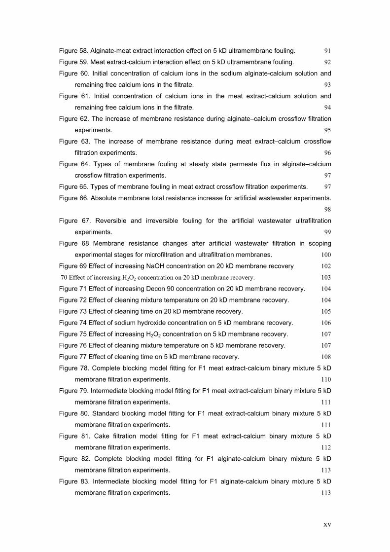
Figure 58. Alginate-meat extract interaction effect on 5 kD ultramembrane fouling. 91

Figure 59. Meat extract-calcium interaction effect on 5 kD ultramembrane fouling. 92

Figure 60. Initial concentration of calcium ions in the sodium alginate-calcium solution and

remaining free calcium ions in the filtrate. 93

Figure 61. Initial concentration of calcium ions in the meat extract-calcium solution and

remaining free calcium ions in the filtrate. 94

Figure 62. The increase of membrane resistance during alginate–calcium crossflow filtration

experiments. 95

Figure 63. The increase of membrane resistance during meat extract–calcium crossflow

filtration experiments. 96

Figure 64. Types of membrane fouling at steady state permeate flux in alginate–calcium

crossflow filtration experiments. 97

Figure 65. Types of membrane fouling in meat extract crossflow filtration experiments. 97

Figure 66. Absolute membrane total resistance increase for artificial wastewater experiments.

98

Figure 67. Reversible and irreversible fouling for the artificial wastewater ultrafiltration

experiments. 99

Figure 68 Membrane resistance changes after artificial wastewater filtration in scoping

experimental stages for microfiltration and ultrafiltration membranes. 100

Figure 69 Effect of increasing NaOH concentration on 20 kD membrane recovery 102

70 Effect of increasing H2O2 concentration on 20 kD membrane recovery. 103

Figure 71 Effect of increasing Decon 90 concentration on 20 kD membrane recovery. 104

Figure 72 Effect of cleaning mixture temperature on 20 kD membrane recovery. 104

Figure 73 Effect of cleaning time on 20 kD membrane recovery. 105

Figure 74 Effect of sodium hydroxide concentration on 5 kD membrane recovery. 106

Figure 75 Effect of increasing H2O2 concentration on 5 kD membrane recovery. 107

Figure 76 Effect of cleaning mixture temperature on 5 kD membrane recovery. 107

Figure 77 Effect of cleaning time on 5 kD membrane recovery. 108

Figure 78. Complete blocking model fitting for F1 meat extract-calcium binary mixture 5 kD

membrane filtration experiments. 110

Figure 79. Intermediate blocking model fitting for F1 meat extract-calcium binary mixture 5 kD


Figure 80. Standard blocking model fitting for F1 meat extract-calcium binary mixture 5 kD


Figure 81. Cake filtration model fitting for F1 meat extract-calcium binary mixture 5 kD


Figure 82. Complete blocking model fitting for F1 alginate-calcium binary mixture 5 kD


Figure 83. Intermediate blocking model fitting for F1 alginate-calcium binary mixture 5 kD


xvi

Figure 84. Standard blocking model fitting for F1 alginate-calcium binary mixture 5 kD


Figure 85. Cake filtration model fitting for F1 alginate-calcium binary mixture 5 kD membrane


Figure 86. Complete blocking model fitting for F1 artificial wastewater mixture 5 kD membrane


Figure 87. Intermediate blocking model fitting for F1 artificial wastewater mixture 5 kD


Figure 88. Standard blocking model fitting for F1 artificial wastewater mixture 5 kD membrane


Figure 89. Cake filtration model fitting for F1 artificial wastewater mixture 5 kD membrane


Figure 90. Complete blocking model fitting for F1 artificial wastewater mixture 20 kD


Figure 91. Intermediate blocking model fitting for F1 artificial wastewater mixture 20 kD

membrane filtration experiments 118

Figure 92. Standard blocking model fitting for F1 artificial wastewater mixture 20 kD


Figure 93. Cake filtration model fitting for F1 artificial wastewater mixture 20 kD membrane


Figure 94. Main effects of wastewater components on intermediate blocking model R2 values

for the 5 kD ultrafiltration membrane. 121

Figure 95. Main effects of wastewater components on complete blocking model R2 values for

the 5 kD ultrafiltration membrane. 123

Figure 96. Main effects of wastewater components on cake–filtration model R2 values for the

5 kD ultrafiltration membrane. 124

Figure 97. Main effects of wastewater components on standard blocking model R2 values for


Figure 98. Main effects of wastewater components on intermediate blocking model R2 values

for the 20 kD ultrafiltration membrane. 127

Figure 99. Main effects of wastewater components on complete blocking model R2 values for


Figure 100. Main effects of wastewater components on cake filtration blocking model R2

values for the 20 kD ultrafiltration membrane. 129

Figure 101. Main effects of wastewater components on standard blocking model R2 values for


Figure 102. Main effects of meat extract-calcium binary mixture components on intermediate

blocking model R2 values for 5 kD membrane filtration. 131

Figure 103. Main effects of meat extract-calcium binary mixture components on complete


xvii

Figure 104. Main effects of meat extract-calcium binary mixture components on cake filtration


Figure 105. Main effects of meat extract calcium binary mixture components on standard


Figure 106. Main effects of alginate-calcium binary mixture components on intermediate


Figure 107. Main effects of alginate-calcium binary mixture components on complete blocking

model R2 values for 5 kD membrane filtration. 135

Figure 108. Main effects of alginate-calcium binary mixture components on cake filtration


Figure 109. Main effects of alginate-calcium binary mixture components on standard blocking

model R2 values for 5 kD membrane filtration. 137

Figure 110. Steady state flux vs. particle diameter for artificial wastewater experiments

calculated using the Song and Elimelech concentration polarisation equation. 139

1

1.0 Introduction

1.1 Global Water Shortage

One of the biggest problems facing the world in this century is the shortage of

potable water, especially in the developing countries. Global water

consumption has increased six fold from 1900 to 1995 (Singh, 2006). The

water shortage is so severe that, according to the World Health Organisation

(WHO), almost 60% of human illnesses are caused by contaminated water or

the lack of sewer treatment (Singh, 2006).

Fresh water is a fundamental need for most aspects of life. Fresh water is

needed in agriculture, for drinking water, or as process water in various

industries. Groundwater and/or surface water is not always sufficiently

available and there are often many impurities contained in water. Water

impurities may be classified by their size (Aptel, 1994):

True solutes: small molecules, with a size less than one nanometre, and

macromolecules with sizes between 1 and 10 nanometres.

Colloidal suspensions: heterogeneous systems, in which the dispersed

compounds generally measure less than 100 nm.

Particles: suspended solids visible under an optical microscope, with sizes

more than 200 nm.

1.2 Water treatment

Water treatment processes are needed to remove these impurities so that

communities can use water safely. A number of classical separation

processes are already used as cleaning technologies, such as sand filtration,

sedimentation, coagulation, flocculation, precipitation, distillation, disinfection,

oxidation and ion exchange. The technique used depends largely on the

specific application, and in many cases more research is needed to determine

the appropriate technique to be applied and on the process parameters.

2

Different kinds of pollution present in waters used for various purposes result

in a situation where their treatment is not easy to perform, and the treatment

system may need to be specified individually for each type of water. In order

to guarantee the quality required of potable water or water used for industrial

purposes, often unconventional or high efficiency processes must be applied

(e.g., membrane techniques) which are expected to improve consumer safety

despite the higher costs involved.

1.3 Membrane Wastewater treatment

Membrane technology offers the advantages of higher effluent quality and a

reduction of treatment plant size compared to traditional wastewater treatment

technology The fouling of membranes by wastewater components is a major

disadvantage, responsible for slowing the implementation of membrane

separation technology in wastewater treatment (Judd and Jefferson, 2003;

Singh, 2006).

In addition to the higher effluent quality and smaller plant footprint of

membrane separation technology, a major advantage is the smaller sludge

volume produced using membrane bioreactor technology in wastewater

treatment (Judd and Jefferson, 2003).

In traditional activated sludge wastewater treatment processes, aggregation of

microbials into flocs, bioflocculation, is a very important and desired process.

Bioflocculation is believed to improve solid/liquid separation, which in turn

leads to improved settling and dewatering in the bioreactor (Sobeck and

Higgins, 2002; Steiner et al., 1976; Houghton et al., 2001).

From an operational point of view, a large amount of excess sludge presents

a serious drawback for wastewater treatment plants (Neyens et al., 2004).

From an economic point of view it is estimated that 25-50 % of wastewater

treatment cost is associated with sludge waste management (Baeyens et al.,

3

1997). Therefore, dewatering of sludge in wastewater plants is a costly as

much as an essential process (Houghton et al., 2001). Membrane bioreactor

technology can reduce the amount of sludge production in wastewater yet

achieve a high quality effluent.

1.4 Research Aims and Objectives The aim of this work is to explore the problem of membrane fouling by

wastewater components in depth. Understanding the effect of changing

wastewater components concentration on membrane fouling, the specific

fouling blocking mechanisms, type of fouling and extant of fouling caused by

different components, will help in solving the membrane fouling problem. The

objectives of this study are:

To relate membrane fouling to wastewater organic and non-organic

components concentration,

To relate membrane fouling mechanisms to wastewater components

concentration,

To relate membrane fouling Type to wastewater components

concentration and

To identify an efficient cleaning procedures.

4

2.0 Literature Review

2.1 Wastewater Technology

2.1.1 Conventional activated sludge process

Recycling and reuse of industrial and municipal wastewater is one way of

dealing with the water shortage problem.

Table 1 lists several undesirable water contaminants, the conventional

solutions for them and corresponding membrane processes that can do the

job.

Table 1 Conventional and membrane process solutions to common water problems. Ho and Sirkar (1992).

Constituents of concern

Conventional Process Membrane Process

Turbidity

Suspended Solids

Biological Contamination

Coagulation/Flocculation

Media Filtration

Disinfection

Microfiltration

Colour

Odour

Volatile Organics

Activated carbons

Media Filtration

Aeration

Ultrafiltration

Hardness

Sulphates

Manganese

Iron

Heavy Metals

Lime Softening

Ion Exchange

Oxidation

Filtration

Coagulation/Flocculation

Nanofiltration

Total Dissolved Solids

Nitrate

Distillation

Ion Exchange

Reverse Osmosis

Electrodialysis

5

Membrane bioreactors (MBR) are increasingly replacing the old conventional

activated sludge process in wastewater treatment plants. Traditional activated

sludge schemes consist of an aeration tank and a secondary clarification tank

(Figure 1).

Figure 1. Conventional activated sludge schematic. Water Environment Federation (2006)

2.2 Membrane technology

Membrane technology has become a significant separation technology over

the last decades of the twentieth century (Judd and Jefferson 2003). The main

strength of membrane technology is the fact that the membrane separation

works without the addition of chemicals, with a relatively low energy use and

easy and well organised process conditions.

The membrane separation process is based on the use of semi permeable

membranes. The membrane acts as a specific filter that will let water flow

through, while retaining suspended solids and other substances. There are

various methods that are used as the driving force to enable substances to

penetrate a membrane. Examples of these are a pressure difference, a

concentration gradient, or an electric potential (Judd and Jefferson, 2003)

Treating high turbidity and high total organic carbon (TOC) municipal

wastewater using membrane filtration gives more stable and superior water

quality compared to coagulation sedimentation techniques (Singh 2006).

6

Membrane filtration can be divided into microfiltration and ultrafiltration on one

hand and nanofiltration and reverse osmosis (RO or hyper filtration) on the

other hand. When membrane filtration is used for the removal of larger

particles (10-0.1 and 0.1-0.001 µm) microfiltration and ultrafiltration are

applied, respectively. Due to the open character of these membranes, the

productivity is high while the pressure differentials are low.

When salts need to be removed from water, nanofiltration or reverse osmosis

are applied (Singh 2006). Nanofiltration and RO membranes do not work

according to the pores size separation; separation takes place by diffusion

through the membrane (Singh 2006). The pressure that is required to perform

nanofiltration and reverse osmosis is much higher than the pressure required

for micro and ultrafiltration, while the productivity is much lower.

Membrane filtration has a number of benefits over existing water purification

techniques. Filtration is a process that can take place at low temperatures.

This is mainly important because this enables the treatment of heat sensitive

matter, thus these methods are widely used for food products. For a high

temperature process (higher than 40 ºC), a ceramic membrane is used (Singh

2006).

Membrane separation processes have low energy costs. Most of the energy

that is required is used to pump liquids through the membrane. The total

amount of energy that is used is minor compared to alternative techniques

such as evaporation. The process can easily be expanded.

2.2.1 Membrane bioreactor

In the MBR system, the aeration and the clarification steps are combined;

they can be pressure driven, in which case the membrane module is located

externally to the bioreactor, or vacuum driven, in which case the membrane

module is submerged in the bioreactor; see Figure 2 (Water Environment

Federation, 2006).

7

Figure 2. External and Immersed MBR Schematic (Water Environment Federation, 2006).

The advantages of using membrane bioreactors to treat industrial and

municipal wastewater are numerous; some of the benefits are (Singh, 2006):

High quality effluent due to complete biomass retention.

Small footprint. The elimination of secondary clarifiers resulting in a

smaller wastewater plant.

Due to the modular nature of the membrane systems they provide ease

of expansion and flexibility in configuration.

Wide range of solids retention time (SRT) operation thus giving

flexibility and greater options to optimise the system operation.

MBR processes can be easily automated resulting in a reduction in

operator requirements.

High quality effluent reduces the need for downstream disinfection.

2.2.2 Membrane structure

Membranes are categorised according to the way by which separation is

achieved (Table 2):

8

Dense: where a high degree of selectivity is achieved. The separation relies

on the physicochemical interactions between the membrane material and the

permeating components.

Porous: the separation is mechanically achieved by size exclusion. Materials

with sizes larger than the pore size are rejected.

Table 2. Dense and porous membranes for water treatment (Judd and Jefferson 2003).

Dense Porous Reverse osmosis (RO) Separation achieved by virtue of differing solubility and diffusion rates of water (solvent) and solutes in water. Electrodialysis (ED) Separation achieved by virtue of differing ionic size, charge and charge density of solute ions using ion exchange membranes. Pervaporation (PV) Same mechanism as RO but with the (volatile) solute partially vapourised across the membrane by partially evacuating the permeate side. Nanofiltration (NF) Formerly called “leaky reverse osmosis”. Separation achieved through a combination of charge rejection, solubility diffusion and sieving through micropores (<2 nm).

Ultrafiltration (UF) Separation by sieving through mesopores (2-50 nm) Microfiltration (MF) Separation of suspended solids from water by sieving through macropores (>50 nm) Gas transfer (GT) Gas transferred under a partial pressure gradient into or out of water in molecular form.

Membrane materials limited to

polymeric materials.

Both polymeric and inorganic

materials available.

The common types of membrane elements used in wastewater treatment are

flat sheet, hollow fibres (Figure 3), tubular and spiral wound (Figure 4) (Water

Environment Federation 2006).

9

Figure 3 Hollow fibre RO membrane module assembly (Singh 2006).

Figure 4 Spiral wound membrane module (Singh 2006).

2.2.3 Membrane materials

Membranes can be categorised as organic (polymeric) or inorganic (ceramic

or metallic) depending on their material composition. Moreover, membranes

can be categorised according to their physical structure (morphology).

10

The morphology of a membrane depends on the material and process in

which they were manufactured. Membranes in which a pressure driven

process is used for their construction are usually anisotropic, which means

that they have symmetry in a single direction. The pore size changes with

depth for an asymmetric membrane. A skin, a thin permselective layer, is to

minimise the hydraulic resistance (Table 3) (Judd and Jefferson, 2003).

Table 3. Membrane materials by type (Judd and Jefferson 2003). Membrane Manufacturing

procedure Applications

Ceramic Stretched polymers Track etched polymers Supported liquid Integral asymmetric, microporous Composite asymmetric microporous Ion exchange

Pressing, sintering of fine powders followed by sol gel coating Stretching of partially crystalline foil Radiation followed by acid etching Formation of liquid film in inert polymer matrix Phase inversion Application of thin film to integral asymmetric microporous membrane to produce TFC Functionalisation of polymer material

MF, UF. Aggressive and/or highly fouling media MF. Aggressive, sterile filtration, medical technology MF (polycarbonate (PET) materials). Analytical and medical chemistry, sterile filtration Gas separations, carrier mediated transport MF, UF, NF, GT NF, RO, PV ED

2.3 Microfiltration and ultrafiltration

The principle of microfiltration and ultrafiltration is physical separation. The

extent to which dissolved solids, turbidity and micro organisms are removed is

determined by the size of the pores in the membranes. Substances that are

larger than the pores in the membranes are fully removed. Substances that

are smaller than the pores of the membranes are partially removed,

depending on the construction of the rejection layer on the membrane.

Typical ranges of particle sizes and membrane processes used to separate

them are described in Figure 5. Microfiltration and ultrafiltration are pressure

11

dependent processes, which remove dissolved solids and other substances

from water to a lesser extent than nanofiltration and reverse osmosis.

Figure 5 The filtration spectrum. Osmonics, Inc. (2002).

2.3.1 Microfiltration

Membranes with a pore size of 0.1 – 10 µm are used to perform

microfiltration. Microfiltration membranes can remove all bacteria. A part of

the viral contamination is removed in the process, even though viruses are

smaller than the pores of a microfiltration membrane. This is because viruses

can attach themselves to a bacterial biofilm. Microfiltration can be

implemented in many different water treatment processes when particles with

diameters greater than 0.1 mm need to be removed from a liquid.

In terms of characteristic particle size, this range covers the lower portion of

the conventional clays and the upper half of the range for humic acids (Judd

and Jefferson, 2003). This is smaller than the size range for bacteria, algae

and cysts, and larger than that of viruses. A distinction should be made here

between ‘dead end filtration’ (where clarified fluid is forced perpendicularly

12

through the filter) and ‘crossflow filtration’ (where the bulk suspension flows

tangentially to the surface of the membrane).

The separation mechanism in microfiltration is based on a sieving

mechanism. This means that the membrane will separate many substances in

the feed solution based on their size compared with the size of the membrane

pores. Substances larger than the pore size will be excluded by the

membrane, while smaller substances will pass through the membrane.

The pressure driven permeate flux through this cake layer and the membrane

may be described by Darcy’s law (Ho and Sirkar, 1992; Coulson et al,. 1991).

)(

1

cmo RR

p

dt

dV

AJ

(2.1)

where J is the permeate flux, V is the total volume of the permeate, t is the

filtration time, Δp is the pressure drop imposed across the cake and

membrane, ηo is the viscosity of the suspending fluid, Rm is the membrane

resistance and Rc is the cake resistance.

2.3.2 Ultrafiltration

For the complete removal of viruses, ultrafiltration is required. The pores of

ultrafiltration membranes can remove particles of 0.001 – 0.1 µm from fluids.

Ultrafiltration can also be applied for pre-treatment of water for nanofiltration

or reverse osmosis.

The most important membrane properties are obviously the flux and the

rejection. The volumetric flux is given by Darcy’s law, while the observed

solute rejection Ri for a given species i is given by (Coulson et al. 1991):

ir

ipi c

cR 1 (2.2)

13

where cip and cir are the concentration in the permeate and retentate sides,

respectively.

Microfiltration and ultrafiltration are used in combination with other membrane

processes. Bodzek et al. (2002) used ultrafiltration as a pretreatment before

water containing chloroform was processed by nanofiltration and reverse

osmosis. Ultrafiltration has also been used for sludge concentration before

dewatering (Ho et al. 1992). The major barrier to the use of ultrafiltration in

water treatment is the cost of the water produced.

2.4 Theories of bioflocculation mechanisms

Three theories exist that describe the mechanisms of cations in

bioflocculation; the Derjaguin, Landau, Verwey, and Overbeek (DLVO) theory,

the Divalent Cation Bridging (DCB) theory, and the Alginate Theory (Sobeck

and Higgins, 2002). In the DLVO theory particles are surrounded with a

double layer of counterions, a first, tightly associated, layer of counterions

called the Stern layer and a second layer of less tightly associated

counterions called the diffuse layer. The negative cloud surrounding the

particles results in repulsion forces between particles. According to this

theory, increasing cation concentration should compress the double layer thus

allowing particles to aggregate.

In the Alginate theory, alginate, which is a polysaccharide made up of a linear

copolymer of monomers of 1-4 linked β-D- mannuronic and α-L-guluronic

acids (Draget et al., 2002), forms a gel in the presence of Ca++. The gel is

formed in what is called an egg-box model (Figure 6). According to this

theory, this model is unique to the alginate composition (Bruus et al., 1992).

Polysaccharides such as alginate are unprotonated at the typical pH of

activated sludge. The unprotonated carboxyl groups contribute to the negative

charge of the biofloc (Frolund et al.,1996; Horan and Eccles, 1986).

14

Figure 6 Alginate calcium cation “egg-box” model (Sobeck and Higgins, 2002). Finally, the DCB theory emphasises the role of cations such as Ca++ and Mg++

in bridging between the negatively charged functional groups of EPS (Figure

7). The bridging causes biopolymers to aggregate into bioflocs (Sobeck and

Higgins, 2002).

Figure 7 Divalent cation bridging (Sobeck and Higgins, 2002).

2.4.1 Effect of particle size and particle size distribution Tarleton and Wakeman (1993) studied the effect of fine particle size and

particle size distribution on flux decline in microfiltration. They found that

15

although smaller particle size resulted in a more rapid flux decline, at longer

filtration times the flux for ‘large’ and ‘small’ particle systems were almost of

the same magnitude (see Figures 8 and 9). This phenomenon was more

noticeable with higher crossflow velocities and higher particle concentrations.

Figure 8 Effect of particle size on flux decline at lower crossflow velocity. Tarleton and Wakeman (1993).

Figure 9 Effect of particle size on flux decline at higher crossflow velocity. Tarleton and Wakeman (1993). Furthermore, Tarleton and Wakeman (1993) reported that unlike conventional

dead end filtration, where small particles form the highest resistance cake, the

lack of static cake formation complicated the identification of the fouling cake

layer structure. Nevertheless, the authors hypothesised that smaller particles

in the feed were mainly responsible for the fouling cake formation (Figure 10).

16

Figure 10 Effect of particle size distribution on flux decline. Tarleton and Wakeman (1993).

2.4.2 Effect of crossflow velocity on microfiltration flux

Zhong et al. (2007) used an ultrafiltration membrane with a pore size of 0.05

μm to recover titanium silicalite (TS-1) catalysts with particle diameters in the

range of 1-7 μm from slurry (Figure 11).

Figure 11 Size distribution of TS-1 particles. Zhong et al. (2007).

The researchers reported that dense cake layers formed on the membrane

surface as a result of the interaction between TS-1 particles, a silica additive

17

and iron precipitation, leading to a large flux decline during the filtration

process (Figure 12).

Figure 12 Effect of iron ions on the decline of flux. Zhong et al. (2007).

The authors reported that although an estimation of hydrodynamic forces

acting on a single TS-1 particle (Figure 13) indicated that crossflow velocity

(CFV) has a significant effect on the deposition of the particle, increasing CFV

after the strong and dense cake layer has formed could not resuspend the

TS-1 particle (Figure 14).

Figure 13 Forces acting on a single particle. Zhong et al. (2007).

18

Figure 14 Effect of crossflow velocities on the decline of flux. Zhong et al. (2007).

2.4.3 Effect of yeast cells on microfiltration flux

Güell et al. (1999) studied the effect of yeast on dead end microfiltration of

protein mixtures. In their work, Güell et al. (1999) used a 0.2 μm cellulose

acetate membrane to filter an equal amounts mixture of bovine serum

albumin, lysozyme and ovalbumin proteins. Yeast was added as suspension

or as a cake on top of the membrane to study its effect. The researchers

reported that a 0.022 g/L yeast concentration in suspension enhanced the

permeate flux and kept the protein transmission at nearly 100% (Table 4).

Table 4 Permeate flux at different times and total permeate. Güell et al. (1999).

Permeate flux (L/m2 h) at different times

(s)

Total

permeate (L)

100 1,800 10,800

Water 9,800±600 9,200±300 n/a n/a

Protein only 10,000±1500 360±100 70±30 0.48±0.03

0.022 g/L Yeast only 10,000±500 1,700±300 600±100 1.40±0.12

0.043 g/L Yeast only 6,900±750 1,300±150 700±50 1.20±0.13

0.28 g/L Yeast only 2,900±600 720±50 450±15 0.65±0.05

Protein+0.022 g/L yeast 8,500±1000 1,600±200 275±150 1.21±0.05

Protein+0.043 g/L yeast 5,300±1000 400±130 50±20 0.36±0.07

Protein+0.18 g/L yeast 3,700±1200 300±150 35±8 0.28±0.09

19

Although the proteins used in their study were much smaller in diameter than

the pores of the microfiltration membrane, the authors attributed the severe

fouling to the denaturation and aggregation of a fraction of proteins in the

mixture. Furthermore, they hypothesised that adding yeast to the suspension

formed a secondary membrane that helped retain protein aggregates (Figure

15).

Figure 15 Proposed mechanisms of protein aggregation (a) without and (b) with yeast cells. Güell et al. (1999). It was found that after plotting the resistance for the protein mixtures with

different yeast concentrations that internal fouling dominates initially and after

some time the external fouling due to cake growth was dominant (Güell et al.,

1999).

2.4.4 Biomass effect on membrane fouling

The effect of biomass characteristics on membrane fouling has also been

studied. In their study, Fane et al. (1981) showed that membrane resistance

increased linearly with the mixed liquor suspended solids (MLSS) content.

Yamamoto et al. (1989) reported that when MLSS concentration exceeded

20

40,000 mg L-1 the flux decreased rapidly in a submerged membrane

bioreactor system.

Different models have been suggested to predict the effect of MLSS on

membrane resistance. Shimizu et al. (1993) described the impact of MLSS on

cake layer resistance as:

bc CvR (2.3)

where α is the specific cake resistance (m kg-1); v is the permeate volume per

unit area (m3 m-2); and Cb is the bulk MLSS or mixed liquor suspended solids

concentration (kg m-3).

The concentration of MLSS in an aerobic MBR usually ranges anywhere from

3,000 to 31,000 mg L-1 (Brindle and Stephenson, 1996); however, Lubbecke

et al. (1995) reported that MLSS concentrations as high as 30,000 mg L-1 were

not responsible for irreversible MBR fouling.

Several researchers have proposed empirical relations predicting the effect of

MLSS concentration on the flux and resistance of an MBR system.

2.4.5 Role of Extracellular Polymeric Substances (EPS) in membrane fouling

Although some studies have not found a clear relationship between the

concentration of extracellular polymeric substances and membrane fouling

(Evenblij et al., 2005), it is generally accepted that EPS, which consists of

biopolymers (polysaccharides, proteins, humic substances and lipids)

produced by microorganisms by cell lysis or active transport, are the major

fouling substance in the membrane bioreactor process (Neyens et al., 2004;

Rosenberger and Kraume, 2003; Rosenberger et al., 2005; Tarnacki et al.,

2005; Katsoufidou et al., 2007; Al-Halbouni et al., 2009; Chang et al., 2002;

Bin et al., 2008; Ye et al., 2005a; Arabi and Nakhla, 2008). EPS constitutes

21

80% of the activated sludge mass (Frolund et al, 1996). Furthermore,

polysaccharides are the major constituent of EPS. Forster (1971a) reported

that polymer extracted from an activated sludge was almost totally

polysaccharide. Another study found that polysaccharides constitute about

60% of EPS (Neyens et al., 2004).

A clear relationship between the concentration of dissolved polysaccharides

and membrane permeate flux under constant filtration conditions has been

found by many researchers (Tarnacki et al., 2005; Rosenberger and Kraume,

2003; Rosenberger et al., 2005; Jarusutthirak et al., 2002; Lesjean et al.,

2005). A decrease in membrane permeate flux was reported with increasing

dissolved polysaccharides concentration (Tarnacki et al., 2005). Other

researchers have reported that sludge filterability always decreased with

increasing suspended EPS concentration (Rosenberger and Kraume, 2002).

Moreover, Rosenberger et al. (2005) reported that the main influence on

membrane performance comes from soluble polysaccharides and organic

colloids.

Proteins are an important component of EPS. Zhou et al. (2007) reported that

proteins and polysaccharides were the major components comprising the

fouling layer. Moreover, Kimura et al. (2005) found that proteins and

polysaccharides were the dominant foulants.

The interaction between the different components of EPS is an interesting

subject to many researchers. Many researchers widely believe that even a

substance having only a minor influence individually might have a larger effect

in a mixed system (Ye et al., 2005b). More severe irreversible fouling caused

by a mixture of alginate, humic acid and calcium compared to the individual

solutions of each of these components was reported (Jermann et al., 2007).

Another study in which the fouling behaviour of bicomponent solutions of

BSA-alginate, alginate-unwashed yeast, washed yeast and alginate-bentonite

were compared with mono-solutions of alginate, BSA, unwashed yeast,

washed yeast and bentonite, found that the alginate-BSA solution caused the

highest irreversible fouling (Negaresh et al., 2007). However, Ye et al. (2005b)

22

did not find a significant difference between the fouling caused by a mono-

solution of alginate and a bicomponent solution of alginate-BSA, although the

fouling of the bicomponent solution was higher than for the BSA mono-

solution.

2.4.6 Role of cations in membrane fouling

The role of divalent cations is an unclear and controversial one. Some

researchers have reported a reduction of membrane fouling with increased

calcium cation concentration (Kim and Jang, 2006). Aspelund et al. (2008)

studied the effect of cationic polyelectrolyte concentration on permeate flux

and rejection of bacterial cell suspension in stirred and unstirred cell, dead

end and crossflow microfiltration, reporting that an increase in the cationic

polyelectrolyte dosage resulted in the formation of larger flocculated particles

and increased membrane permeate flux (Aspelund et al., 2008; Nguyen et al.,

2008b). On the other hand, several studies on the interaction effects of

cations, especially divalent calcium cations and EPS components such as

polysaccharides, proteins and humic acids, have reported that they form

complexes with the organic molecules that form a compacted fouling layer on

the membrane surface, causing severe flux decline (Costa et al., 2006; Hong

and Elimelech, 1997; Schäfer et al., 1998; Li and Elimelech, 2004; Yoon et al.,

1998). To complicate the matter further, Arabi and Nakhla (2008) reported

that using a control membrane bioreactor (MBR) with a calcium concentration

of 35 mg/L and two test MBRs with calcium concentrations of 280 mg/L and

830 mg/L respectively, the first MBR fouled the membrane less than the

control MBR while the second test reactor, with the highest calcium

concentration, fouled the membrane the most. The researchers speculated

that cationic bridging with EPS by the calcium created a larger floc size in the

first test MBR that improved permeate flux and lowered the fouling, whilst the

excess of calcium cations in the second test MBR led to significant inorganic

fouling.

23

It seems that the disagreement between researchers is not limited to stating

either that cations improve or worsen membrane fouling in the presence of

EPS but also extend to what type of fouling is caused by their interaction with

EPS. Some researchers reported an increase in the reversibility of the

membrane fouling with increasing calcium concentration, attributing this to the

elimination of EPS adsorption onto the membrane and the cake fouling

becoming the controlling fouling, with increased flocculation influenced by

increased calcium cation concentration (Katsoufidou et al., 2007). Other

researchers have reported opposite behaviours (van de Ven et al., 2008;

Abrahamse et al., 2008). In a surface water ultrafiltration study by Abrahamse

et al., (2008) the authors found that irreversible fouling increased linearly with

increasing calcium and magnesium concentrations.

2.4.7 Morphology effects on membrane fouling

Hwang and Lin (2002) studied the effects of polymeric micro filtration

membrane morphology on crossflow performance. In this study three

membranes, MF Millipore (made of mixed cellulose esters), Durapore (made

of modified polyvinylidene difluoride) and Isopore (made of bisphenol

polycarbonate), with the same mean pore size of 0.1 µm were used (Figure

16).

Figure 16 Modelling of pore structures of the three membranes used. Hwang and Lin (2002).

24

Three blocking mechanism models were reported: a standard blocking, with

particles deposited on the surface of the membrane and completely blocking

the entrances of the pores, with the MF Millipore membrane; an intermediate

blocking, in which the particles are almost the same size as the membrane

pores; therefore, the particles may either be deposited at the entrances or

migrate inside the pores of the membrane, in the Durapore membrane; and, in

the case of the Isopore membrane, a complete blocking, in which the particle

size is smaller than the membrane pore size thus most of the particles migrate

inside the membrane pores causing irreversible fouling. For all the

membranes the blocking model translated to cake filtration within 10 minutes.

In their study, Faibish and Cohen (2001) showed that a permeability decline of

less than 2 per cent after cleaning was achieved for a polyvinylpyrrolidone

(PVP) modified zirconia based ultrafiltration membrane. A permeability decline

of 17 per cent was observed for the non-modified zirconia based ultrafiltration

membrane. Nevertheless, it is worth noticing that the clean membrane

permeability of the PVP modified zirconia based membrane was 48% less

than the native non-modified clean membrane (Table 5).

Table 5. Hydraulic permeability (kt) of membranes. Faibish and Cohen (2001). Component kt (10-16 m2)

clean membranekt (10-16 m2) after

filtration and cleaning

Reduction%

(a) 4% (by vol.) isobutanol 0.002 M octanoic acid

0.5 M sodium octanoate (>GMC)

0.3 M sodium octanoate (>GMC)

Microemulsion

7.39 7.39 7.39

7.08

4.40

7.38 7.27 6.12

5.62

3.47

< 1 2

17 21 26

(b) 0.5 M sodium octanoate

(>GMC) 0.5 M sodium octanoate

(>GMC)

3.40

3.39

3.39

3.37

< 1 < 1

(c) Native membrane

Modified membrane

7.00 3.39

5.80 3.33

17 < 2

25

The reduction associated with the modified membrane may suggest that the

modification process resulted in the formation of a cake layer on the

membrane surface, thus a better control of the irreversible fouling was

achieved.

The PVP modified membrane improved the rejection of an oil and its

microemulsion by 100 and 20 per cent, respectively Faibish and Cohen

(2001). The authors attributed the improvement in the rejection rate to a

repairing or narrowing effect of the polymer grafting process on the defects or

“pin-holes” of the zirconia based membrane.

2.4.8 Intermittent effects on membrane fouling

In their study, Chua et al. (2002) examined the possibility of controlling fouling

in an MBR caused by a temporary permeate flux increase by increasing the

aeration rate. They concluded that membrane fouling can be eliminated when

the permeate flux was reduced back to the sub critical rate. Moreover, the

researchers concluded that the intermittent permeation technique was

effective in reducing the fouling in an MBR operating above the critical flux

rate.

2.4.9 Reversible and irreversible fouling There is some disagreement between researchers on the definition of

reversible and irreversible fouling. Some researchers consider limiting the

definitions of membrane fouling to irreversible and reversible fouling as

somewhat simplistic (Chang et al., 2002). Nevertheless, in general

researchers consider irreversible fouling as that which cannot be removed

with physical cleaning but can be removed by chemical cleaning (Ye et al.,

2005; Judd and Jefferson, 2003; Abrahamse et al., 2008). In this work, the

following definitions of reversible and irreversible fouling were adopted: any

fouling that can be removed without chemical cleaning is considered

26

reversible and fouling removed by chemical cleaning is considered irreversible

fouling.

2.5 Membrane cleaning methods

There is several different membrane cleaning methods in common use, such

as forward flush, backward flush and air flush.

2.5.1 Physical cleaning

2.5.1.1 Forward flush

When a forward flush is applied, membranes are flushed with feed water or

permeate in the forward direction. The feed water or permeate flows through

the system more rapidly than during the production phase. Due to of the more

rapid flow and the resulting turbulence, particles that are absorbed onto the

membrane are released and discharged. The particles that are absorbed into

membrane pores are not released. These particles can only be removed

through backward flushing. When a forward flush is applied to a membrane,

the barrier that is responsible for dead end management is opened. At the

same time the membrane is temporarily performing crossflow filtration, without

the production of permeate.

The purpose of a forward flush is the removal of an accumulated layer of

contaminants on the membrane through the creation of turbulence. A high

hydraulic pressure gradient is in order during a forward flush.

2.5.1.2 Backward flush

Backward flush is a reversed flow process. Permeate is flushed from the

permeate side of the system under pressure to the retentate side, applying

twice the flux that is used during filtration. When the flux has not been

sufficiently restored after back flushing, a chemical cleaning process can be

applied.

27

When backward flush is applied the pores of a membrane are flushed inside

out. The pressure on the permeate side of the membrane is higher than the

pressure within the membranes, causing the pores to be cleaned. A backward

flush is executed under a pressure that is about 2.5 times greater than the

production.

Permeate is always used for a backward flush, because the permeate

chamber must always be free of contamination. A consequence of a

backward flush is a decrease in the recovery of the process. A backward flush

therefore must take the smallest possible amount of time and consume as

little permeate as possible. However, the flush must be maintained long

enough to fully flush the volume of a module at least once.

In their study, Zhong et al. (2007) used different sizes and concentrations of

micro sized alumina particles for physical cleaning of a fouled microfiltration

ceramic membrane. The authors reported a very good cleaning result with

different sizes of alumina particles, especially with the 25 μm particles (Figure

17). The cleaning efficiency with the alumina particles increased with

increasing alumina particle concentration (Figure 18).

Figure 17. Effect of alumina particle size on recovery of flux. Zhong et al. (2007).

28

Figure 18. Effect of alumina concentration on recovery of flux. Zhong et al. (2007).

The authors further reported that a particle cleaning combined with an acid

cleaning restored the membrane flux fully (Figures 19 and 20).

Figure 19. SEM micrograph of fouled membrane. Zhong et al. (2007).

29

Figure 20. SEM micrograph of membrane after cleaning. Zhong et al. (2007).

2.5.2 Chemical cleaning processes When the above mentioned cleaning methods are not effective to restore the

flux to an acceptable level, chemical cleaning of the membranes is necessary.

During a chemical cleaning process, membranes are soaked with a solution of

chlorine bleach, hydrochloric acid or hydrogen peroxide. First the solution

soaks into the membranes for several minutes and after that a forward flush

or backward flush is applied, causing the contaminants to be rinsed out.

During chemical cleaning, chemicals such as hydrogen chloride (HCl) and

nitric acid (HNO3), or disinfection agents, such as hydrogen peroxide (H2O2)

are added to the permeate during backward flush. As soon as the entire

module is filled with permeate, the chemicals need to soak in. After the

cleaning chemicals have fully soaked in, the module is flushed and, finally, put

back into production thus insuring the removal of all the cleaning chemicals

used.

Cleaning methods are often combined. For example, one can use a backward

flush for the removal of pore fouling, followed by a forward flush or air flush.

The cleaning method or strategy that is used is dependent on many factors. In

practice, the most suitable method is determined by trial and error (practical

tests).

30

In their study, Zhong et al. (2007) started a chemical cleaning procedure to

clean a microfiltration membrane by rinsing the filtration system with deionised

water, followed by circulating a 1% (v/v) sodium hydroxide solution, then

circulating a 1% (v/v) nitric acid solution, both at temperature of 80 °C, for

several hours while keeping the permeate line open (Figure 21).

The filtration system was finally rinsed with deionised water. Furthermore,

Zhong et al. (2007).took advantage of the high thermal stability of the ceramic

membrane to remove organic foulants by baking the fouled ceramic

membrane for one hour at a temperature of 500 °C. The Zhong et al. (2007).

reported that EPS analysis showed no organic matter in the cake layer and

membrane pores after the baking procedure. Moreover, Zhong et al. (2007).

reported an increase in the pure water flux from 230 L/(m2 h) to 247 L/(m2 h)

for the fouling membrane after the high temperature baking procedure. The

researchers hypothesised that the high temperature was responsible for

removing all organic matter by volatilisation (Zhong et al. 2007).

Figure 21. Variation of flux with cleaning time. Zhong et al. (2007).

31

2.5.3 Biofilm removal A biofilm is a layer of micro organisms contained in a matrix (a slime layer),

which forms on surfaces in contact with water. Incorporation of pathogens in

biofilms can protect the pathogens from concentrations of biocides that would

otherwise kill or inhibit those organisms if freely suspended in water.

Biofilms provide a safe haven for organisms like Listeria, E. coli and

Legionella where they can reproduce to levels where contamination of

products passing through that water becomes inevitable. Chlorine dioxide has

been proven to remove biofilms from water systems and prevents them from

forming when dosed at a continuous low level; Hypochlorite on the other hand

has been proven to have little effect on biofilms (Li et al., 2005).

2.6 Crossflow membrane filtration modelling

In membrane ultrafiltration, the flux is usually distinguished as being in one of

two regimes: a non steady state, in which flux declines with time, and a steady

state where the flux is constant (Song, 1998).

The rate of initial flux decline and the final steady state flow is dependent on

the fouling mechanisms involved and the operating conditions such as trans

membrane pressure, flow velocity, shear rate, feed concentration and feed

temperature. However, the effects of operating parameters are not very clear

even after numerous experimental studies and are sometimes contradictory

(Tarleton and Wakeman, 1993).

2.7 Dead end blocking models

The flux reduces with time in a membrane filtration process due to fouling.

The three main mechanisms that effect membrane permeate flux are

complete blocking, standard blocking and cake formation (Figure 22).

32

Figure 22. Membrane blocking mechanisms. In his study, Hermia (1982) started with a dead end filtration equation and

adapted it to predict the reduction of permeate flux in crossflow filtration.

For the three different blocking mechanisms, the proposed models for

complete blocking, standard blocking, cake and intermediate blocking,

respectively, are as follows:

EtkJ

Jb

0

ln (2.4)

0

1

2 Jt

K

V

t b (2.5)

0

1

2 JV

K

V

t k (2.6)

0

11

JtK

J i (2.7)

where J and 0J are the permeate and clean water fluxes respectively, V is

permeate volume collected at time t, and bK , kK and iK are constants.

Several models have been developed to predict the flux decline in membrane

filtration. A critical factor in most of these models is the particle size. Hermia’s

Complete blocking

Standard blocking

Cake filtration

33

blocking flows are constructed on the basis of the difference between particle

size and membrane pore size. Although Hermia’s pore blocking and cake

formation models were developed for dead end filtration, they can be used to

understand the blocking mechanisms for crossflow filtration experiments

(Jiraratananon et al., 1998; Mohammadi et al., 2003).

Several researchers have modified Hermia’s flow to better suit crossflow

filtration configurations (Vela et al., 2009; Field et al., 1995; Bowen et al.,

1995). The main consideration in the modified models is that they account for

the back diffusion of solutes from the membrane surface to the bulk flow.

2.7.1 Combined blocking mechanisms models

Since the possibility exists for more than one blocking mechanism occurring

at the same time, an attempt has been made by some researchers to

combine some of the blocking models to give a better description of the

experimental data. Bolton et al. (2006) formulated five constant pressure

combined fouling models as the following:

Cake filtration and complete blocking model:

121exp11 2

2tJK

JK

K

K

JV oc

oc

b

b

o (2.8)

where the fitted parameters are Kc (s/m2) and Kb (s-1)

Cake filtration and intermediate blocking model:

1211ln

1 2/12tJKJK

K

KV oc

oc

i

i

(2.9)

where the fitted parameters are Kc (s/m2) and Ki (m-1)

34

Complete blocking and standard blocking model:

tJK

tK

K

JV

os

b

b

o

2

2exp1 (2.10)

where the fitted parameters are Kb (s-1) and Ks (m

-1)

Intermediate blocking and standard blocking model

tJK

tJK

KV

os

oi

i 2

21ln

1 (2.11)

where the fitted parameters are Ki (m-1) and Ks (m

-1)

3

1arccos

3

1

3

2cos

2 sK

V (2.12)

c

s

oc

s

K

tK

JK

K3

2

33 3

4

3

4

27

8

,

c

s

oc

s

K

tK

JK

K

3

2

3

4

9

4 2

where the fitted parameters are Kc (s/m2) and Ks (m-1)

Prádanos et al. (1996) modified the pore blocking models for crossflow

filtration. In the complete blocking model, particles block some of the

membrane pores with no superposition of particles and the permeate flux

decline with time is given by:

0,lnln vbv JtKJ (2.13)

where Kb is the complete blocking kinetic constant (s-1)

35

In the intermediate blocking model, particles can settle on top of other

particles that are already blocking membrane pores or they can block open

membrane pores by themselves. The flux decline with time is given by:

tK

JJ

i

vv

10, (2.14)

where Ki is the intermediate blocking kinetic constant (s-1)

The standard blocking model accounts for the possibility that particles arriving

at the membrane surface are smaller than the pore diameter and can deposit

on the internal pore walls, thus reducing the pore volume. The flux decline

with time is given by:

2

0,

1 tK

JJ

s

vv

(2.15)

where Ks is the standard blocking kinetic constant (s-1)

Finally, the cake filtration model assumes that particles arriving at the

membrane surface are deposited on top of other particles and there is no

room for contact with the membrane area. The flux decline with time is given

by:

tK

JJ

c

vv

1

0, (2.16)

where Kc is the cake filtration kinetic constant (s-1)

In complex mixtures such as wastewater, the particle size distribution is very

wide, thus the use of a single blocking mechanism for calculating flux decline

is an unrealistic approach.

2.7.2 Concentration Polarisation Theory In a membrane crossflow filtration process, particles with sizes larger than the

membrane pore size are rejected by the membrane. During this process the

particles rejected by the membrane accumulate near the membrane surface.

36

The concentration of the rejected particles near the membrane surface

becomes higher than the concentration of the particles in the bulk, thus

creating what is called the concentration polarisation layer.

In their research, Song and Elimelech (1995) proposed a new method for

predicting the formation of a concentration polarisation layer and calculating

permeate flux. The researchers proposed a new dimensionless number,

called the filtration number, FN ; this number can be calculated using Equation

2.17:

kT

PaN p

F 3

4 3

(2.17)

where:

pa is the particle size

P is the transmembrane pressure

K is the Boltzmann constant

T is the absolute temperature

The filtration number represents the ratio of the energy required to move the

particle from the membrane surface back to the bulk solution to the thermal

energy of the particle. The researchers reported a critical value for the

filtration number. When the value of the filtration number is less than the

critical value, a polarisation layer will exist over the membrane surface (Figure

23). Conversely, if the filtration number value is higher than the critical value,

a cake layer is formed between the concentration polarisation layer and the

membrane surface (Figure 24).

37

Figure 23. Concentration polarisation layer over a membrane surface.

Figure 24. Cake layer between CP layer and membrane surface.

38

3.0 Equipment and Experimental Methods

In this chapter the artificial wastewater composition and mixing procedure, the

filtration apparatus design and filter element, the dead end stirred cell filtration

apparatus and samples analyses procedures are described.

3.1 Artificial wastewater composition

In this study, an artificial wastewater was used. Real wastewater is a complex

unstable mixture with continuously changing living micro-organisms making it

unsuitable for controlled experiments. The need for stable artificial wastewater

was widely recgdnized by different researchers (Sanin and Vesilind, 1999;

Örmeci and Vesilind, 2000; Nguyen et al., 2008). The artificial wastewater

composition was as described by Lu et al (2001); furthermore, sodium alginate

was added to simulate the effect of soluble microbial products (SMP); see

Table 6.

Table 6. Artificial wastewater compositions Lu et al (2000). Substance Concentration, mg/L wt %

Na alginate 100 9.90

Peptone 180 17.82

Meat extract 180 17.82

Urea 30 2.97

NH4Cl 70 6.93

(NH4)2CO3 160 15.84

NaCl 20 1.98

K2HPO4 90 8.91

CaCl2·2H2O 35 3.47

KCl 110 10.89

MgCl2·6H2O 35 3.47

39

The main components in the wastewater which it was believed would have

the most effect on membrane fouling are alginate, peptone, meat extract and

CaCl2·2H2O. Throughout this study, the concentration of these compounds

was varied to examine their effects on the membrane fouling rate.

3.2 Artificial wastewater preparation procedure

For each experiment, the amount of each component in the artificial

wastewater was measured using a four decimal sensitive balance. The

correct weight for each component was then dispersed into a 2 L beaker filed

with ultra pure water from a Millipore reverse osmosis purification system.

Once all components were added and stirred, the suspension was transferred

to the filtration apparatus feed tank where fresh ultra pure water was added to

obtain a total volume of around 20 litres in the feed tank.

3.3 Artificial wastewater characterisation

The artificial wastewater in this study was characterised with respect to

particle size distribution, solids concentration, density, viscosity, shear rate

and Zeta potential.

The particle size distribution of the artificial wastewater was characterised

using a Malvern MS20 Mastersizer. The particle size measurement was done

to characterise the particle size distribution of the artificial wastewater for each

experiment, to ensure that all compounds in the artificial wastewater feed

were adequately dispersed, and that no major changes in the particle size

distribution occurred in all the experiments with the same component

concentrations.

40

3.3.1 The Malvern Mastersizer

The Malvern Mastersizer works on the principle of the laser diffractometer,

where the laser light from the instrument is scattered by the particles in the

suspension depending on their size and light scattering characteristics. The

scattered light is focused onto an array of sensors. The data from the sensors

are processed by a computer that calculates the particle size distribution. The

lens and focal length for the instrument should be selected according to the

particle sizes in the suspension and the presentation factor was chosen in

accordance with the Mastersizer instruction manual.

3.3.2 Zeta potential measurement

The Zeta potential for each artificial wastewater mixture was measured using

a Malvern Zetamaster. The Zeta potential measurement gave an indication of

the tendency of the compounds in the artificial wastewater to agglomerate at a

certain pH, and was used to ensure the similarity of the artificial wastewaters

used in all the experiments.

The Malven Zetamaster measures the speed at which charged particles move

through an electrical field via a laser light and a light sensor. The Zetamaster

relates the speed to the particle surface charge, thus calculating the Zeta

potential of the particles.

The Malven Zetamaster is computer controlled and equipped with an auto

titrator filled with hydrochloric acid and sodium hydroxide. After specifying the

range of pH at which to test the solution, the auto titrator changes the artificial

wastewater solution pH according to a chosen range and measures the Zeta

potential at different pH values. The pH and corresponding Zeta potential of

the artificial wastewater solution are recorded automatically.

41

3.4 Experimental crossflow filtration apparatus

A diagram of the crossflow filtration apparatus is shown in (Figure 25). The

artificial wastewater mixture was loaded into the 20 L stainless steel feed

tank. The artificial wastewater was feed to the membrane filter element by a

constant flow centrifugal pump. The pump was a 0.5 HP Lowara CKM70/3

rated at 2,850 rpm. The pump was capable of delivering maximum pressure

of 5 bars. The pressures at the membrane module inlet as well as the

membrane outlet were both measured by two Farnell MM10013 pressure

transducers.

The temperature of the wastewater feed to the membrane module was

monitored by thermocouples. The computer controlled the temperature of the

wastewater via a hot water jacket surrounding the wastewater feed tank.

The membrane module inlet and outlet pressures, feed tank temperature, and

membrane module inlet wastewater feed temperature were automatically

recorded by a data logging system. The permeate flux was measured

manually. The crossflow filtration apparatus could be operated in a constant

concentration mode by returning the permeate back to the feed tank or

concentration mode by removing the permeate from the filtration system.

42

Figure 25. Crossflow filtration apparatus.

3.5 Apparatus control

The major equipment in the crossflow filtration apparatus were controlled via a

computer program written in Visual Basic. The computer program controlled

the following:

1. The apparatus main pump

2. The feed tank mixer

3. The heating elements

4. The heating water loop pump.

Moreover, the computer program recorded the following:

1. Membrane module inlet and outlet pressures

43

2. Feed tank temperature

3. Membrane module wastewater feed inlet temperature.

3.5.1 Membrane filter element

In this research, two Atech ceramic membrane elements were used for the

artificial wastewater filtration experiments. A 1 m long α-Al2O3 microfiltration

membrane with a pore size of 0.2 µm and two 1 m long TiO2 ultrafiltration

membrane elements with pore sizes of 20 and 5 kDa were used in this study.

All the membranes were single channel tubular ceramic membranes with an

outer diameter of 10 mm and a 6 mm internal diameter. Each ceramic

membrane filter was installed in a stainless steel housing and sealed by

rubber O-rings at each end. The module (housing and membrane element)

was mounted vertically in the filtration apparatus and secured by flanges at

both ends and sealed with plastic gaskets.

3.5.2 Filtration apparatus piping and fittings

The apparatus pipework, fitting, ball valves, feed tank and built in water jacket

were all of stainless steel. A 20 mm terylene mesh reinforced PVC tubing was

used to return the retentate to the feed tank. The filter permeate was returned

to the feed tank via a polypropylene tube when operating in constant

concentration mode.

3.5.3 Filtration apparatus temperature control

Water in an insulated storage tank was heated by 3 kW heating elements.

This hot water was then pumped around the wastewater feed tank hot water

jacket. The wastewater feed temperature was measured by RS PT100

thermocouples. The temperature of the wastewater was maintained at a user

44

defined set point by turning the heating elements on or off as required by the

computer control program.

3.6 Experimental procedures

3.6.1 Wastewater mixture filtration experiments

3.6.1.1 Factorial design of the experiments

The ultrafiltration experiments were designed using a full two level factorial

design statistical method described in Appendix D. Four factors, sodium

alginate, peptone, meat extract and calcium chloride, were selected for study

at high and low concentrations to determine their effects on the wastewater

filtration process (Table 7).

Table 7 Four factor, two level designs. factor High (mg/L) Low (mg/L) Sodium alginate 150 50 Peptone 270 90 Meat extract 270 90 CaCl2·2H2O 60 20

Sixteen experiments plus the central experiment (Table 8) were required to

investigate all the possible combinations of the high and low concentrations of

the four factors under investigation.

In all sixteen experiments and the central experiment, the effects of the

changes in the factor (component) levels (concentrations) on a measured

response (Y) such as flux, COD, TOC and membrane resistance were

45

recorded. The results were analysed as a set of equations (Equation 3.1) that

was solved for the factors effect βs.

Table 8 Full factorial, two level experimental design runs.

Experiment Peptone (mg/L)

Meat Extract (mg/L)

Sodium Alginate (mg/L)

CaCl2 2H2O (mg/L)

F1 90 270 150 20

F2 270 270 150 20

F3 270 90 50 20

F4 90 270 150 60

F5 270 90 150 20

F6 270 90 150 60

F7 90 90 150 20

F8 90 270 50 20

F9 270 270 50 60

F10 270 270 150 60

F11 90 90 50 20

F12 90 90 150 60

F13 270 270 50 20

F14 90 90 50 60

F15 270 90 50 60

F16 90 270 50 60

Y = β0 + β1 X1 + β2 X2 + β3 X3 + β4 X4 + β12 X1 X2 + β13 X1 X3 + β14 X1 X4 + β23

X2 X3 + β24 X2 X4 + β34 X3 X4 + β123 X1 X2 X3 + β124 X1 X2 X4 + β134 X1 X3 X4 +

β234 X2 X3 X4 + β1234 X1 X2 X3 X4 (3.1)

46

where:

X1 = Peptone concentration (mg/L)

X2 = Meat extract concentration (mg/L)

X3 = Sodium alginate concentration (mg/L)

X4 = Calcium chloride concentration (mg/L)

3.6.1.2 Measurement of clean water flux

The clean membrane flux measurement was carried out after installing the

new membrane using ultra pure water to establish the membrane resistance

(Rm). The flux of the new membrane was taken at different pure water

temperatures, flow rates and trans membrane pressures.

The clean water flux was measured before the start of every wastewater

filtration experiment to record any change to the membrane resistance.

3.6.1.3 Measurement of experimental flux

The following procedures were followed for all experimental runs.

Start of Experiment; Clean water flux measurement:

1. The feed tank was filled with twenty litres of clean ultra pure water.

2. The heater set point temperature was set to 40 °C and the water was

heated to this temperature.

3. The pump was started and the permeate side valve was opened.

4. Three flux measurements were taken.

5. The pump was stopped and the feed tank drain valve was opened to

empty the feed tank.

Artificial wastewater preparation and wastewater filtration experiment:

47

1. The artificial wastewater chemical components were measured using a

sensitive balance.

2. The components were dissolved in 10 litres of ultra pure water in a

bucket.

3. The artificial wastewater was mixed for 60 minutes using a mixer.

4. The artificial wastewater was loaded into the filtration apparatus feed

tank and diluted with 10 litres of ultra pure water to obtain a total

volume of 20 litres of artificial wastewater in the feed tank.

5. The filtration apparatus mixer was started.

6. The temperature set point was set to 40 °C and the heaters were

turned on in the apparatus computer control programme.

7. The pump was turned on and the artificial wastewater was circulated in

the filtration apparatus with the permeate side valve closed for about

10 minutes.

8. The permeate side valve was opened and permeate was recycled to

the feed tank.

9. The permeate flux was measured by collecting samples at pre

determined time intervals. Permeate volume was measured using a

measuring cylinder and a stopwatch to record the time for each

sample.

10. Permeate sample volume and time were manually recorded throughout

the duration of the experiment and the permeate samples were

returned to the feed tank after the measurements, except for samples

at 5, 30, 80, 120 and 180 minutes, for which 8 mL samples were taken

for laboratory analysis.

End of Experiment:

1. The pump was stopped.

2. The drain valve was opened to empty the feed tank.

End of Experiment; Clean water flux measurement:

1. The feed tank was filled with twenty litres of clean ultra pure water.

2. The heater set point temperature was set to 40 °C and the water was

heated to this temperature.

48

3. The pump was started and the permeate side valve was opened.

4. Three flux measurements were taken.

5. The pump was stopped and the feed tank drain valve was opened to

empty the feed tank.

Apparatus cleaning after wastewater experiments:

1. The cleaning solution was filled into the feed tank.

2. The heater set point was set to 50 °C.

3. The pump was started and the cleaning solution was circulated through

the filtration apparatus for 60 to 90 minutes.

4. The pump was stopped and the cleaning solution was kept in the

filtration apparatus for 10 minutes before it was drained via the drain

valve.

5. The filtration apparatus was flushed with tap water twice for 5 and 15

minutes each.

6. Finally, the feed tank was filled with ultra pure water and the pump was

started to circulate the water through the membrane for 30 minutes.

7. The pump was stopped and the inlet valve to the membrane housing

was closed to keep the membrane wet.

8. The computer was shut down and the main power to the filtration

apparatus was turned off.

3.6.1.4 Total Organic Carbon (TOC) and Inorganic Carbon (IC) Measurement

The ThermoEuroglas Total Organic Carbon analyser, TOC 1200, uses a non

dispersive infrared detector (NDIR) to measure the amount of CO2 produced

by a sample oxidised in the high temperature furnace and relates the amount

of CO2 to the concentration of total carbon in the sample.

The liquid sample is injected into a boat that introduces the sample to the

analyser high temperature furnace, set at 1000 °C. The sample is flushed with

argon during the boat movement to the furnace so volatile components will

49

enter the furnace. The sample is oxidised with oxygen gas. The oxidation

products are led through a copper oxide scrubber then though the inorganic

carbon scrubber, after which the oxidation products pass through a Perma

pure dryer. The oxidation product gases pass through a particle filter before

finally flowing into the NDIR detector, which measures the concentration of

CO2. The area of the signal measured by the NDIR detector is used to

calculate the TOC concentration.

In the TOC 1200 analyser, a sample can be introduced at either of two places:

boat injection, to measure the total carbon, TC, or IC scrubber injection for

inorganic carbon, IC, measurement.

Total organic carbon (TOC) and inorganic carbon (IC) concentrations were

determined as follows:

1. TC measurement via boat injection

2. IC measurement via IC scrubber injection

3. TOC Calculated as TC – IC = TOC

The ThermoEuroglas Total Organic Carbon analyser, TOC 1200 was

calibrated with known standards to establish a calibration curve for analysing

the filtration experiment samples (Figures 26 and 27).

y = 0.0004x2 - 0.0736x + 29.239

R2 = 0.9973

0100200300400500600700800900

10001100

0 200 400 600 800 1000 1200 1400 1600 1800 2000

Area

Co

nce

ntr

atio

n (

mg

/l)

Figure 26. Total carbon calibration for the TOC 1200 Analyser.

50

y = 0.0007x2 - 0.0415x + 30.302

R2 = 0.9988

0100200300400500600700800900

10001100

0 200 400 600 800 1000 1200

Area

Co

nce

ntr

atio

n (

mg

/l)

Figure 27. Inorganic carbon calibration for the TOC 1200 Analyser.

3.6.1.5 Chemical Oxygen Demand (COD) measurement Ready to use Palintest reagent tubes with sulphuric acid and potassium

dichromate in the presence of a silver sulphate catalyst were used to oxidise

the water sample by digestion. The reduction in the amount of potassium

dichromate is proportional to the COD in milligrams of oxygen consumed per

litre of sample (Palintest Photometer Instruction Manual, 2007).

The amount of Cr3+ formed from the reduction of potassium dichromate was

used to indirectly measure the COD of the water sample according to:

3422

272 2

2

38)8( dCrcNHOH

cdanCOHcdOdCrNOHC cban

where: 2363

2 cband

3.6.1.6 Phosphate measurement An optical method was used to determine the concentration of phosphate in

the artificial wastewater feed and permeate samples. Palintest® Photometer

7100 and Phosphate HR reagent tablets were supplied by Palintest, Ltd. The

test is based on the vanadomolybdate method in which the intensity of yellow

colour of the phosphovanadomolybdate produced by the reaction of

51

phosphates with ammonium molybdate in the presence of ammonium

vanadate is proportional to the concentration of phosphate (Palintest

Potometer 7100 Instructions Manual 2007).

Test Procedure:

1. A test tube is filled with 10 mL of the water sample.

2. One tablet of Phosphate HR reagent is added, crushed and mixed to

dissolve.

3. The sample is allowed to stand for 10 minutes to allow full colour

development.

4. The test tube is inserted into the photometer tube holder.

5. The Phot 29 automatic wavelength programme is selected.

6. The photometer reading is displayed as mg/L PO4.

3.7 Bicomponent dead end stirred cell filtration experiments

3.7.1 Sodium alginate and calcium chloride dihydrate solution preparation

A 1000 mg/L solution of sodium alginate was prepared by dissolving 0.5 gram

of brown algae alginic acid sodium salt (Fluka Chemie AG) in 500 mL of

Millipore Milli Q system purified water.

A 1000 mg/L solution of calcium chloride dihydrate was prepared by

dissolving 0.5 grams of calcium chloride dihydrate (Fisher Scientific, USA) in

500 mL Millipore Milli-Q system purified water.

Solutions with different concentrations of sodium alginate and calcium

chloride dihydrate were prepared by combining the appropriate volumes of

both solutions and diluting to 100 mL with Milli-Q purified water.

The Sodium alginate calcium mixture preparation procedures were as follows.

Sodium alginate and calcium stock solution preparation:

52

1. Prepare 500 mL of 1000 mg/L sodium alginate solution:

a. Dissolve 0.5 grams of sodium alginate powder in 500 mL of

deionised water.

b. Mix and stir for two hours

2. Prepare 500 mL of 1000 mg/L Ca++ solution:

a. Dissolve 0.5 grams of calcium chloride in 500 mL deionised

water.

b. Mix and stir for two hours

Preparation of different sodium alginate-calcium solutions:

1. For a 300 mg/L sodium alginate /100 mg/L calcium solution:

a. Mix 30 mL of the 1,000 mg/L sodium alginate solution with 10

mL of the 1,000 mg/L calcium chloride solution.

b. Dilute to 100 mL with deionised water

c. Stir for 30 min

2. For a 300 mg/L sodium alginate /80 mg/L calcium solution:

a. Mix 30 mL of the 1,000 mg/L sodium alginate solution with 8 mL

of the 1,000 mg/L calcium chloride solution.


c. Stir for 30 min.

3. For a 300 mg/L sodium alginate / 60 mg/L calcium solution:




c. Stir for 30 min.


53




c. Stir for 30 min.





c. Stir for 30 min

Table 9. Sodium alginate and calcium chloride solutions.

Solution concentration (mg/L)

CaCl2 solution (mL)

Alginate (mL)

Purified water (mL)

[Alg.] = 300, [CaCl2] = 20 2 30 68 [Alg.] = 300, [CaCl2] = 40 4 30 66 [Alg.] = 300, [CaCl2] = 60 6 30 64 [Alg.] = 300, [CaCl2] = 80 8 30 62

[Alg.] = 300, [CaCl2] = 100 10 30 60

3.7.2 Meat extract and calcium chloride dihydrate solution preparation:

A 1000 mg/L solution of meat extract was prepared by dissolving 0.5 gram of

meat extract (Oxoid, Ltd., England) in 500 mL Millipore Milli-Q system purified

water.

A 1000 mg/L solution of calcium chloride dihydrate was prepared by

dissolving 0.5 grams of calcium chloride dihydrate (Fisher Scientific, USA) in

500 mL Millipore Milli-Q system purified water.

Solutions with different concentrations of meat extract and calcium chloride

dihydrate were prepared by combining the appropriate volumes of both

solutions and diluting to 100 mL with Milli-Q purified water.

54

The meat extract-calcium mixture preparation procedure was as follows.

Meat extract and calcium stock solution preparation:

1. Prepare 500 mL solution of 1,000 mg/L meat extract:

a. Dissolve 0.5 grams of meat extract powder in 500 mL deionised

water.

b. Mix and stir for two hours.

2. Prepare 500 mL solution of 1,000 mg/L Ca++:

a. Dissolve 0.5 grams of calcium chloride in 500 mL deionised

water.

b. Mix and stir for two hours.

Preparing different meat extract-calcium solutions:

1. For a 300 mg/L meat extract / 100 mg/L calcium solution:

a. Mix 30 mL of the 1,000 mg/L meat extract solution with 10 mL of

the 1,000 mg/L calcium chloride solution.


c. Stir for 30 min





c. Stir for 30 min



the 1,000 mg/L calcium chloride solution


55

c. Stir for 30 min.





c. Stir for 30 min





c. Stir for 30 min

Table 10. Meat extract and calcium chloride solutions. Solution concentration

(mg/L) CaCl2

solution (mL)

Meat Ex. (mL)

Purified water (mL)

[Meat Ex.] = 300, [CaCl2] = 20 2 30 68 [Meat Ex.] = 300, [CaCl2] = 40 4 30 66 [Meat Ex.] = 300, [CaCl2] = 60 6 30 64 [Meat Ex.] = 300, [CaCl2] = 80 8 30 62 [Meat Ex.] = 300, [CaCl2] = 100 10 30 60

3.7.3 Stirred cell filtration experiments A 50 mL Millipore stirred cell with a 47 mm ultrafiltration membrane disc filter

was used to filter the sodium alginate and calcium chloride solutions and the

meat extract and calcium chloride solutions.

For the sodium alginate and calcium chloride experiments, a 47 mm

polyethersulfone ultrafiltration membrane with an NMWL cut-off of 10,000

Daltons (Millipore Corporation, USA) was used to filter the solution. For the

meat extract and calcium chloride experiments, an OMEGA 47 mm

polyethersulfone ultrafiltration membrane with a MWCO of 1,000 Daltons (Pall

56

Life Sciences, USA) was used to filter the solutions. Both disc membranes

had an effective filtration area of 17.3 cm2.

3.7.4 Membrane preparation The membranes were washed by soaking for 24 hours in Milli-Q system

purified water. Membranes were rinsed upon installation by passing 50 mL of

purified water through the stirred cell to remove any impurities and additives

used during the manufacturing process, as recommended by the

manufacturer.

3.7.5 Stirred cell ultrafiltration experiment The stirred cell was loaded with 50 mL of the solution to be filtered, a nitrogen

gas line was connected to the stirred cell and the two way valve was opened.

The pressure in the stirred cell was monitored by a pressure gauge and

controlled using a model 8286 pressure regulator (Porter Instrument Co.,

USA). All filtrations were conducted using a TMP pressure of 1.25 bars and

room temperature (Figure 28).

Figure 28. Stirred cell ultrafiltration

57

3.7.6 Calcium cation concentration analysis Atomic absorption spectroscopy was used to measure free calcium cation

concentration in the solution. A Varian atomic absorption spectrophotometer

(model SpectrAA 200; Varian Australia Pty., Ltd.) was used (Figure 29).

Elemental metals absorb UV when they are in an excited state. Although

atoms exist in a stable state called the ground state in normal conditions,

atoms can be transformed to higher excited state by some processes such as

the addition of thermal energy.

Figure 29. Atomic absorption spectrophotometer. In the atomic absorption spectroscopy instrument, a nebuliser aspirates the

sample into a flame. The flame provides calcium atoms with the thermal

energy needed to be transferred to an excited state. Upon making that

transition calcium atoms absorb some of the light of the beam (Figure 30).

The lamp generates a beam of light specific for the metal analysed. In the

case of calcium the light beam wavelength is 442.7 nm (Varian Australia Pty.,

Ltd. SpectrAA 200 Manual, 1989). The light beam travels through the flame to

the detector where some of the light is absorbed by the excited calcium

58

atoms. The reduction of light is recorded by the detector. The instrument

compares the reduction in the light intensity to the reduction obtained by a

known concentration in a standard calibration curve and calculates the

sample calcium concentration.

Hollow Cathode lamp

Atomized sample Flame Detector

Figure 30. Simplified atomic absorption spectroscopy apparatus schematic.

3.8 Bicomponent mixture cross-flow filtration experiments

3.8.1 Factorial design of the experiments

A full two level factorial design setup was used for the bicomponent

ultrafiltration experiments. The two level factorial design statistical method

was described in Appendix D.

Two bicomponent mixtures were tested with five experiments run for each

mixture at different concentrations. Sodium alginate-calcium mixture and meat

extract-calcium mixtures were selected for study at high and low

concentration to determine their single and interaction effects on the fouling of

the ultrafiltration membrane (Table 11).

Table 11. High and low concentrations for the two level design factors. factor High (mg/L) Low (mg/L)

Sodium alginate 150 50 Meat extract 270 90 CaCl2·2H2O 60 20

59

Four experiments plus the central experiment were required to investigate all

the possible combinations of the high and low concentrations for the two

bicomponent mixtures under investigation (Tables 12 and 13).

Table 12. Sodium alginate-calcium mixture full factorial, two level

experimental design runs.

Experiment Sodium alginate (mg/L) CaCl2·2H2O (mg/L)

1 100 40

2 50 20

3 150 20

4 50 60

5 150 60

Table 13. Meat extract-calcium mixture full factorial, two level experimental design runs.

Experiment Meat extract (mg/L) CaCl2·2H2O (mg/L)

1 180 40

2 90 20

3 270 20

4 90 60

5 270 60

60

4.0 Results and Discussion In this chapter the result of the microfiltration scoping experiments, the 20 and

5 kD ultrafiltration experiments are described in detail. The flux results of the

filtration experiments as will as the samples analysis results are examined in

detail to determine the effect of changing the artificial wastewater components

concentration.

4.1 Wastewater mixture microfiltration scoping experiments

4.1.1 Filtration flux The reduction in the flux with time (Figure 31) suggests that one of the pore

blocking mechanisms affected the filtration process. The quality of the

permeate COD did not change throughout the filtration experiments which

indicated that the feed particles size is smaller than the membrane pore size

thus allowing the artificial wastewater components to flow to the permeate

side.

0.00

50.00

100.00

150.00

200.00

250.00

300.00

350.00

400.00

0 2000 4000 6000 8000 10000 12000 14000 16000 18000

Time (s)

Jw

(L

/m^

2 h

)

Clean water flux

Figure 31. Flux vs. time for a microfiltration experiment.

61

4.1.2 COD and TOC analyses The microfiltration experiment result clearly shows that the artificial

wastewater component particle sizes were much smaller than the microfilter

membrane pore size. The COD analysis of the feed and permeate samples

(Table 14) show the same values indicating that no separation was achieved

by the 0.2 µm microfiltration membrane.

A smaller pore size membrane was selected to examine the effect of the

different size components on the membrane fouling therefore, ultrafiltration

membranes with pore size of 20 and 5 kilo Dalton were selected to carry on

the rest of the artificial wastewater filtration experiments.

Table 14. COD analysis results for microfiltration wastewater experiment.

Sample Time (min) COD (ppm) Feed - 340 ± 20

1 5 350 ± 10 2 15 360 ± 10 3 30 350 ±10 4 50 360 ± 00 5 75 350 ±10 6 105 330 ± 10 7 140 340 ± 00 8 180 330 ± 10 9 240 340 ± 20 10 300 330 ± 20

End feed - 310 ± 10

4.2 Artificial wastewater mixture 20 kD ultrafiltration

experiments

4.2.1 Flux analysis

The flux decline for experiments F4, F10 and F12, of 78, 78 and 77 per cent,

respectively, was the highest among the artificial wastewater filtration

62

experiments performed. In these experiments, the calcium concentration was

at the high level 60 ppm (Table 8). On the other hand, the flux decline for

experiments F7, F1 and F2 which were conducted with a low calcium

concentration level of 20 ppm had the lowest flux decline recorded, 61, 63 and

63 per cent respectively. This behaviour supports the hypothesis of the

bridging effect of calcium on proteins and polysaccharides proposed by

Katsoufidou et al. (2007).

Table 15. Initial and final permeate flux and membrane resistance for 20 kD membrane artificial wastewater experiments.

Experiment Jcw (L/m2 h)

Jss (L/m2 h)

Rcw (1/m)

Rss (1/m)

F0 1,443 376 4.00E+11 1.56E+12 F1 1,274 475 5.36E+11 1.33E+12 F2 1,198 447 4.98E+11 1.36E+12 F3 1,656 551 3.54E+11 1.08E+12 F4 1,697 373 3.43E+11 1.58E+12 F5 1,515 482 3.82E+11 1.25E+12 F6 1,644 444 3.50E+11 1.44E+12 F7 1,166 452 4.92E+11 1.31E+12 F8 1,783 463 3.52E+11 1.30E+12 F9 1,601 418 3.58E+11 1.40E+12

F10 1,499 335 3.51E+11 1.59E+12 F11 1,601 427 3.50E+11 1.35E+12 F12 1,317 304 3.61E+11 1.82E+12 F13 1,440 385 4.04E+11 1.52E+12 F14 1,508 411 3.82E+11 1.41E+12 F15 1,498 440 3.80E+11 1.30E+12 F16 1,621 402 3.58E+11 1.48E+12

Although experiments F1 and F2 had higher alginate, peptone and meat

extract concentrations than experiments F14 and F15, the reduction in

normalised flux was less compared to experiments F14 and F15 in which the

calcium concentrations were higher even though the concentration of alginate,

peptone and meat extract were low (Table 20).

The concentration of calcium had more effect on the flux reduction than the

change in concentration of the other factors.

63

4.2.2 TOC analyses

The highest feed total carbon (TC) concentration used was in the artificial

wastewater mixture for experiment numbers F2, F10 and F13, in which all the

factors (components) were at high level, except for F13, in which alginate

level was low. The wastewater feed used in experiments F11 and F14, where

meat extract, peptone and alginate were all at low concentration, registered

the lowest concentration of TC. Further, F7 gave a low TC feed result where

the alginate concentration level was high, which indicate that the major source

of TC were meat extract and peptone (Table 16).

The highest reduction of TC concentration was obtained in experiments F7,

F12 and F14. The lowest separation for total carbon was noted in experiments

F9, F13 and F15, in which either meat extract or alginate or both were at low

concentration in the wastewater feed (Table 16).

Table 16. Total carbon analysis results for 20 kD membrane artificial wastewater experiments. Experiment Feed

(ppm) Permeate

sample # 1 Permeate sample# 4

Permeate sample #

6

ΔTC (%)

F0 127±0 95.5±0.7 95.1±0.9 95.3±0.8 25 F1 N/A N/A N/A N/A N/A F2 302.5±3.1 235.4±6.5 243.3±6.2 225.6±8.8 25 F3 215.0±117 171.6±7.3 164.8±14.5 161.5±9.9 25 F4 241.3±1.9 166.7±8.6 161.5±4.4 169.6±2.4 30 F5 267.6±9.7 170.5±4.0 164.5±9.9 178.3±5.7 33 F6 245.0±15.6 181.7±3.0 179.8±11.7 169.6±0.5 31 F7 151.0±1.8 97.2±1.3 92.2±5.9 98.5±0.8 35 F8 199.6±2.1 163.4±3.3 167.0±1.3 167.5±3.8 16 F9 285.1±3.0 254.1±2.2 253.1±10.9 250.5±1.1 12

F10 331.4±2.0 258.4±5.0 250.2±10.5 258.6±5.9 22 F11 136.7±6.6 105.2±2.4 99.2±1.7 99.5±0.9 27 F12 205.8±1.7 110.5±0.2 108.4±3.0 108.0±0.5 48 F13 302.5±10.1 269.5±10.3 264.2±0.2 266.6±5.0 12 F14 173.6±12.3 118.1±6.5 113.8±1.8 114.3±3.6 34 F15 246.5±6.1 213.6±10.3 213.5±17.5 222.6±5.0 10 F16 275.8±10.3 218.3±12.4 201.1±4.2 221.2±1.6 21

64

The reduction of inorganic carbon by the membrane separation was the

lowest of all the parameters measured in this study, indicating that the major

concentration of inorganic carbon in the artificial wastewater existed as CO3-

ions formed by the disassociation of ammonium carbonate (NH4 2CO3), which

is too small to be separated by the ultrafiltration membrane.

Table 17. Inorganic carbon analysis results for 20 kD membrane artificial wastewater experiments.

Experiment Feed (ppm)

Permeate sample # 1

Permeate sample # 4

Permeate sample # 6

F0 28.80±0 26.7±0.1 26.7±0.1 26.5±0.1 F1 46.1±1.4 48.7±3.7 51.7±1.0 50.2±1.7 F2 46.4±3.1 48.3±1.1 45.5±0.6 42.8±1.1 F3 45.8±2.2 45.4±2.3 44.4±0.5 44.7±2.4 F4 47.7±1.2 49.1±0.2 52.0±5.3 48.6±2.8 F5 48.5±2.2 48.1±0.1 45.8±1.0 49.1±2.8 F6 48.6±0.9 45.8±4.1 49.9±6.4 45.7±0.3 F7 46.3±0.6 44.6±0.1 44.2±0.1 44.9±1.0 F8 46.7±0.0 44.6±0.1 45.8±0.4 43.0±0.5 F9 46.5±0.7 46.1±0.8 46.4±0.1 47.8±0.8

F10 48.0±0.9 46.3±0.2 45.8±0.1 48.8±1.7 F11 48.4±0.0 45.4±0.0 41.9±2.7 46.5±0.2 F12 49.9±0.5 47.6±0.9 48.9±0.2 45.3±0.7 F13 49.5±1.8 48.3±0.6 49.6±1.0 48.1±0.6 F14 52.7±0.4 46.5±4.5 52.6±1.9 46.0±0.5 F15 53.3±1.2 51.9±1.5 51.6±1.4 45.7±0.1 F16 50.5±6.4 52.3±0.7 58.7±4.6 57.1±1.0

4.2.3 COD analyses

The highest chemical oxygen demand for the artificial wastewater feed was

used in the feed for experiments F1 and F7, in which all factors (components)

except for calcium were at the high level (concentration) (Table 18).

Furthermore, the highest COD reduction by the filtration process was

achieved in experiments F7 and F12, at 39% and 53%, respectively. In

experiments F7 and F12, the alginate was at high concentration. Moreover,

the COD reduction in experiments F9, F13, F14 and F16 was very low at

65

14%, 17%, 18% and 15%, respectively. The alginate concentration was at a

low level in the experiments where low COD reduction in the permeate was

observed. The large size of the alginate molecules may be responsible for

fouling the membrane and reducing the organic concentration on the

permeate side.

Table 18. Chemical oxygen demand (COD) analysis results for 20 kD membrane artificial wastewater experiments.


Permeate sample

# 1

Permeate sample

# 4

Permeate sample

# 6 F0 460 ± 10 333 ± 6 357 ± 21 360 ± 10 F1 467 ± 6 290 ± 0 303 ± 6 297 ± 6 F2 693 ± 6 510 ± 0 523 ± 6 540 ± 10 F3 447 ± 6 380 ± 0 377 ± 6 360 ± 10 F4 493 ± 6 317 ± 6 337 ± 6 343 ± 6 F5 543 ± 6 357 ± 6 380 ± 0 377 ± 6 F6 513 ± 6 363 ± 6 380 ± 0 373 ± 6 F7 323 ± 6 210 ± 10 203 ± 6 197 ± 6 F8 453 ± 6 363 ± 6 350 ± 0 347 ± 6 F9 673 ± 6 577 ± 6 567 ± 12 577 ± 6

F10 703 ± 6 540 ± 0 523 ± 6 510 ± 0 F11 267 ± 6 203 ± 6 207 ± 6 187 ± 6 F12 250 ± 0 117 ± 6 117 ± 6 117 ± 6 F13 627 ± 6 517 ± 12 517 ± 6 523 ± 6 F14 233 ± 6 170 ± 0 173 ± 6 190 ± 0 F15 450 ± 0 370 ± 0 360 ± 0 363 ± 6 F16 373 ± 6 300 ± 0 317 ± 6 317 ± 6

4.2.4 Phosphate analyses The highest concentration of phosphate was observed in experiments F0, F1

and F2, in which the meat extract was at high concentration level (Table 19).

The lowest value of phosphate concentration was in experiments F3, F5 and

F7, in which the concentration of meat extract and were both at low levels. It

is worth noting that although experiment F4 has a low concentration of

peptone and a high concentration of alginate the concentration of phosphate

in the permeate was low, perhaps due to the high concentration of calcium.

The bridging effect of calcium may have caused an increase in the size of the

proteins due to aggregation, thus increasing their rejection by the membrane.

66



Permeate sample

# 1

Permeate sample

# 4

Permeate sample

# 6 F0 105.7±3.4 88.2±0.5 87.7±0.2 85.8±0.4 F1 103.7±3.0 86.4±0.5 86.6±0.4 83.4±0.5 F2 106.7±1.2 83.7±1.7 79.0±1.6 85.9±0.4 F3 57.5±2.8 43.5±0.4 40.6±0.1 37.2±0.0 F4 77.1±1.9 46.3±0.2 46.3±0.2 45.0±0.5 F5 45.4±0.5 43.8±0.3 22.5±0.2 20.8±0.2 F6 101.8±0.4 68.7±1.4 62.2±0.2 64.6±0.3 F7 58.3±1.2 44.5±0.3 41.3±0.2 42.9±0.2 F8 72.8±1.2 67.0±0.3 67.5±0.3 65.8±0.3 F9 95.6±1.3 91.5±1.3 87.9±0.7 84.1±0.4

F10 91.8±0.8 78.1±1.2 73.1±0.9 70.3±0.4 F11 61.8±0.0 42.1±0.2 39.3±1.4 40.2±2.4 F12 90.4±5.4 62.5±0.7 55.2±0.2 70.7±0.9 F13 98.3±2.3 84.1±1.8 75.1±1.9 87.5±0.3 F14 59.9±0.3 45.1±0.2 41.3±0.1 41.8±0.4 F15 89.1±1.3 68.4±0.3 70.5±0.3 74.6±0.4 F16 87.6±2.1 73.3±0.2 71.2±0.3 67.3±0.6

Table 20. Results of 20 kD ultrafiltration experiments component concentration in (mg/L) responses in reduction percentage from feed.

Run

Peptone (ppm)

Meat extract (ppm)

Alginate (ppm)

CaCl2

(ppm)Δflux (%)

ΔCOD (%)

ΔTC (%)

ΔPO4-

(%) F0 180 180 100 40 74 22 25 19 F1 90 270 150 20 63 36 N/A 20 F2 270 270 150 20 63 22 25 19 F3 270 90 50 20 67 19 25 35 F4 90 270 150 60 78 30 30 42 F5 270 90 150 20 68 31 33 54 F6 270 90 150 60 73 27 31 37 F7 90 90 150 20 61 39 35 26 F8 90 270 50 20 74 23 16 10 F9 270 270 50 60 74 14 12 12 F10 270 270 150 60 78 27 22 23 F11 90 90 50 20 73 30 27 35 F12 90 90 150 60 77 53 48 22 F13 270 270 50 20 73 17 12 11 F14 90 90 50 60 73 18 34 30 F15 270 90 50 60 71 19 10 16 F16 90 270 50 60 75 15 20 23

67

4.3 Artificial wastewater mixture 5 kD ultrafiltration

experiments

4.3.1 Flux analysis

The highest flux reductions were observed in experiments F2, F4 and F15,

while the lowest flux reductions were in experiments F3, F5, F8 and F11, all of

which had low concentration levels of calcium and alginate, except for

experiment F5, where the alginate concentration level was high (Table 21).

Table 21. Initial and final permeate flux and membrane resistance for 5 kD membrane artificial wastewater experiments.

Experiment Jcw (L/m2 h)

Jss (L/m2 h)

Rcw (1/m)

Rss (1/m)

F0 1,329 380 4.44E+11 1.61E+12 F1 1,456 386 3.94E+11 1.55E+12 F2 1,455 367 3.92E+11 1.62E+12 F3 1,371 471 4.27E+11 1.26E+12 F4 1,520 361 3.86E+11 1.62E+12 F5 1,384 443 4.19E+11 1.36E+12 F6 1,392 399 4.16E+11 1.51E+12 F7 1,470 430 3.85E+11 1.40E+12 F8 1,234 443 4.77E+11 1.36E+12 F9 1,323 392 4.46E+11 1.53E+12

F10 1,423 379 4.02E+11 1.66E+12 F11 1,454 465 3.94E+11 1.29E+12 F12 1,287 392 4.50E+11 1.43E+12 F13 1,340 341 4.27E+11 1.71E+12 F14 1,456 380 3.97E+11 1.53E+12 F15 1,739 424 3.34E+11 1.43E+12 F16 1,365 383 4.13E+11 1.56E+12

4.3.2 TOC analyses

The highest feed TC concentration was obtained in experiments F2, F9 and

F10; these experiments had high levels meat extract and peptone

concentrations. Experiments F7 and F12 gave the highest reduction in TC

concentrations in the permeate; in both experiments, meat extract and

68

peptone concentrations were low and alginate concentration was high. Due to

the fact that the major TC concentration was from alginate in experiments F12

and F7, with high alginate concentration and low meat extract and peptone

concentration, the rejection of the large alginate molecules by the 5 kD

membrane led to a higher reduction of TC in the permeate (Table 22).

The major source of inorganic carbon in the artificial wastewater mixture was

ammonium carbonate (NH4·2CO3), and there was no major reduction in the

concentration of inorganic carbon in the permeate (Table 23).

Table 22. Total carbon analysis results for 5 kD membrane artificial wastewater experiments. Experiment Feed

(ppm) Permeate

sample # 1 Permeate

sample # 4 Permeate

sample # 6 F0 253.9±2.1 174.2±5.9 179.9±3.3 173.9±3.2

F1 253.8±4.1 193.7±5.9 179.4±0.4 180.6±1.3

F2 352.2±6.4 258.2±11.2 277.9±1.9 275.9±1.2

F3 215.9±0.4 201.0±3.2 188.8±8.8 185.3±0.5

F4 298.7±1.3 216.4±10.7 198.3±0.4 211.1±2.9

F5 267.8±23.5 195.2±9.9 178.7±1.8 180.3±3.8

F6 273.0±6.6 191.3±8.6 190.3±6.1 173.8±0.9

F7 209.1±1.0 140.1±4.0 119.8±2.3 122.8±3.2

F8 205.5±1.9 170.0±4.2 158.7±0.1 166.7±4.7

F9 316.7±17.5 266.8±12.0 271.6±11.0 270.3±14.4

F10 360.4±5.3 267.2±1.0 273.7±1.0 273.1±0.2

F11 163.9±2.6 129.7±5.9 120.1±2.5 119.4±1.0

F12 181.0±6.2 106.5±3.0 110.7±4.9 103.4±0.9

F13 312.4±6.9 241.8±2.9 234.9±1.9 241.2±5.4

F14 136.4±5.5 106.7±2.2 98.2±1.8 94.5±1.3

F15 288.5±3.1 238.3±4.1 226.5±1.0 226.0±4.8

F16 251.8±1.9 197.5±2.0 201.1±1.1 201.3±5.9

69

Table 23. Inorganic carbon analysis results for 5 kD membrane artificial wastewater experiments. Experiment Feed

(ppm) Permeate

sample # 1 Permeate

sample # 4 Permeate

sample # 6 F0 53.9±1.3 50.2±0.2 51.4±1.2 48.1±1.0

F1 55.9±2.2 47.7±0.5 35.9±1.8 49.5±0.1

F2 48.5±2.3 45.5±9.1 45.3±0.9 46.6±1.4

F3 62.3±1.7 55.1±3.3 50.2±1.3 51.4±0.7

F4 53.7±1.8 53.7±0.7 46.9±6.0 46.5±6.2

F5 53.1±4.7 51.4±1.8 42.5±0.7 46.2±1.0

F6 58.8±3.0 54.4±1.4 50.9±8.1 52.1±3.5

F7 50.2±2.1 49.8±0.9 45.9±7.2 44.1±2.4

F8 51.5±0.4 48.3±3.0 46.2±1.2 46.0±1.4

F9 55.0±1.9 53.7±2.0 53.5±0.4 46.3±2.3

F10 59.3±1.6 51.5±1.9 55.4±2.6 47.9±2.9

F11 51.6±0.8 48.5±7.9 49.1±3.8 46.1±5.6

F12 47.4±0.5 46.3±3.2 44.8±1.5 45.0±0.4

F13 50.9±2.3 46.8±0.4 46.8±1.4 45.0±0.6

F14 57.2±3.0 54.2±4.1 50.1±1.2 48.2±0.5

F15 54.8±0.2 52.4±7.0 53.9±6.0 50.1±2.8

F16 53.9±0.4 50.2±0.3 51.4±1.3 48.1±0.0

4.3.3 COD analyses

Among the experiments with high concentrations of meat extract, peptone and

alginate (F2, F9, F10 and F13), the highest COD concentration reductions

were obtained in the experiments with high alginate concentration and low

meat extract and peptone concentration due to the rejection of alginate by the

membrane (Table 24).

70

Table 24. Chemical oxygen demand (COD) analysis results for 5 kD membrane artificial wastewater experiments.


Permeate sample # 1

Permeate sample # 6

F0 450 ± 0 357 ± 6 360 ± 0

F1 433 ± 6 297 ± 6 293 ± 6

F2 677 ± 6 513 ± 6 510 ± 0

F3 413 ± 6 347 ± 15 353 ± 6

F4 460 ± 0 310 ± 0 330 ± 0

F5 477 ± 6 317 ± 6 337 ± 6

F6 470 ± 0 293 ± 6 330 ± 10

F7 303 ± 6 N/A 170 ± 0

F8 380 ± 10 317 ± 6 333 ± 6

F9 620 ± 10 543 ± 6 520 ± 0

F10 587 ± 6 430 ± 10 433 ± 12

F11 210 ± 0 163 ± 6 173 ± 6

F12 277 ± 10 167 ± 6 187 ± 12

F13 660 ± 0 N/A 520 ± 0

F14 207 ± 6 157 ± 6 163 ± 6

F15 470 ± 0 N/A 363 ± 6

F16 420 ± 10 350 ± 10 370 ± 10

4.3.4 Phosphate analyses

The highest reduction of phosphate in the permeate, at 37%, was found in

both experiments F7 and F12; alginate concentration in the feed wastewater

was also at the same high concentration level of 150 ppm in both

experiments. The lowest phosphate reduction was found in experiments F9,

F13 and F16, at 17%, 15% and 7%, respectively. In all these experiments, the

concentration level of alginate was low, at 50 ppm. The rejection of alginate

by the 5 kD membrane for experiments with high alginate concentration

(making it the major source of phosphate) resulted in a greater fractional

reduction of phosphate concentration in the permeate (Table 25).

71



Permeate sample # 1

Permeate sample # 6

F0 81.7±0.2 61.2±0.7 65.8±0.4 F1 84.9±1.6 57.3±0.5 66.0±0.2 F2 74.5±0.9 52.3±0.1 47.7±1.5 F3 84.3±0.5 61.7±0.7 68.2±0.1 F4 94.3±3.1 68.4±0.2 67.6±1.0 F5 93.5±1.7 66.8±0.4 68.4±0.3 F6 97.2±0.8 65.9±0.3 68.4±0.3 F7 62.9±1.4 42.8±0.2 39.6±1.3 F8 68.6±0.7 60.4±0.1 68.6±0.4 F9 60.0±0.4 47.7±0.2 49.7±1.1

F10 80.3±4.7 54.1±0.2 52.8±0.7 F11 65.2±1.2 48.8±0.6 43.8±1.5 F12 68.4±0.6 44.1±0.4 43.1±1.2 F13 96.8±0.9 88.9±1.7 82.1±0.6 F14 57.1±1.3 45.7±0.1 40.5±0.3 F15 86.1±1.1 69.8±0.7 70.0±1.2 F16 81.0±1.5 69.5±1.5 75.1±0.9

Table 26. Results of 5 kD ultrafiltration experiments: component concentration responses as percentage reductions from the feed. Run

Peptone

(ppm)

Meat extract (ppm)

Alginate

(ppm)

CaCl2

(ppm)

Δflux (%)

ΔCOD (%)

ΔTC (%)

ΔPO4-

(%) F0 180 180 100 40 71 20 32 19 F1 90 270 150 20 73 32 29 22 F2 270 270 150 20 75 25 22 36 F3 270 90 50 20 66 15 14 19 F4 90 270 150 60 76 28 29 28 F5 270 90 150 20 68 29 33 27 F6 270 90 150 60 71 30 36 30 F7 90 90 150 20 71 44 41 37 F8 90 270 50 20 64 12 19 0 F9 270 270 50 60 70 16 15 17 F10 270 270 150 60 73 26 24 34 F11 90 90 50 20 68 18 27 33 F12 90 90 150 60 70 32 43 37 F13 270 270 50 20 75 21 23 15 F14 90 90 50 60 74 21 31 29 F15 270 90 50 60 76 23 22 19 F16 90 270 50 60 72 12 20 7

72

4.3.5 Particles size, pH and Zeta potential measurements The artificial wastewater particles size, pH and zeta potential were measured.

Although both pH and zeta potential have not changed noticeable for all the

factorial experiments, the particle size of artificial wastewater did change with

different artificial wastewater experiments. The change in the particle size

indicates an effect of changing calcium cations concentration which promotes

aggregation of alginate and meat extract (Table 27).

Table 27 Artificial wastewater Particles size, pH and Zeta potenrial Experiment Zeta (mV) pH Size (µm)

F0 -33.1 8.31 N/A F1 -35.3 8.36 N/A F2 -37.5 8.34 7.62 F3 -40.5 8.37 N/A F4 -25.7 8.26 N/A F5 -40.1 8.3 7.35 F6 -30.5 8.19 9.98 F7 -39.6 8.46 6.53 F8 -35.5 8.46 9.97 F9 -30.5 8.3 5.62 F10 -31.4 8.31 5.03 F11 -41.2 8.34 5.25 F12 -23.1 8 4.41 F13 -33.4 8.3 6.78 F14 -30.4 8.38 12.3 F15 -29.7 8.31 7.62 F16 -25 8.35 6.87

4.4 Effects of wastewater component concentrations on membrane fouling factorial design analysis

The membrane resistance increase was calculated by dividing the membrane

resistance at steady state flux, Rss, by the clean membrane resistance

calculated using the pure water flux measurement, Rcw.

73

% Membrane resistance increase = 100CW

SS

R

R (4.1)

4.4.1 Component main effects for 20 kD ultrafiltration membrane wastewater experiments

4.4.1.1 Effect of changing the calcium chloride concentration on membrane fouling

Each two experiments with the same concentrations of all other artificial

wastewater components and high or low calcium concentration (Table 28)

were compared by their percentages of membrane fouling (Figure 32).

Table 28. Equivalent wastewater experiments with different calcium concentration levels.

Experiments Peptone (ppm)

Meat extract (ppm)

Sodium alginate (ppm)

High level Calcium 60 ppm

Low level Calcium 20 ppm

90 270 150 F4 F1 270 270 150 F10 F2 270 90 50 F15 F3 270 90 150 F6 F5 90 90 150 F12 F7 90 270 50 F16 F8 90 90 50 F14 F11

270 270 50 F9 F13

The change in calcium concentration had a great effect on the membrane

fouling. Experimental runs with high calcium levels resulted in a large increase

in membrane fouling, of about 45 per cent on average, compared to

experiments conducted with low calcium concentrations (Figure 33). Among

all the components in the artificial wastewater, changes in the calcium level

had the highest and clearest effect on membrane fouling.

74

0

50

100

150

200

250

300

350

400

450

F1 - F4 F2 - F10 F3 - F15 F5 - F6 F7 - F12 F8 - F16 F11 - F14 F13 -F9

Experiments

Me

mb

ran

e re

sist

anc

e in

ceas

e % [Ca] = 20 ppm

[Ca] = 60 ppm

Figure 32. Equivalent wastewater experiments with high and low calcium concentrations; membrane fouling results.

604020

320

300

280

260

240

220

Calcium Concentration (ppm)

Mem

bran

e re

sist

ance

incr

ease

(%

)

CornerCenter

Point Type

Figure 33. Average membrane resistance increase for experiments with high and low calcium concentrations.

75

4.4.1.2 Effect of changing the sodium alginate concentration on membrane fouling


wastewater components and high or low sodium alginate concentration (Table

29) were compared by their percentages of membrane fouling (Figure 34).

Table 29. Equivalent wastewater experiments with different sodium alginate concentration levels.


Meat extract (ppm)

Calcium (ppm) High level

Alginate 150 ppm

Low level Alginate 50

ppm 270 90 20 F5 F3 90 270 20 F1 F8

270 270 60 F10 F9 90 90 20 F7 F11

270 270 20 F2 F13 90 90 60 F12 F14

270 90 60 F6 F15 90 270 60 F4 F16

The fouling behaviour of sodium alginate was similar to that of meat extract.

Changes in the concentration level of alginate did not result in noticeable

changes in the membrane fouling (Figure 35). A high level of alginate gave

more fouling than was observed in experiments with low alginate

concentrations; however, it was a very small increase.

76

0

50

100

150

200

250

300

350

400

450

F3 - F5 F8 - F1 F9 - F10 F11 - F7 F13 - F2 F14 - F12 F15 - F6 F16 - F4

Experiments

Mem

bra

ne

resi

stan

ce i

nce

ase

%

[Alginate] = 50 ppm

[Alginate] = 150 ppm

Figure 34. Equivalent wastewater experiments with high and low alginate concentrations; membrane fouling results.

15010050

290

285

280

275

270

Concentration (ppm)

Mem

bran

e re

sist

ance

incr

ease

(%

)

CornerCenter

Point Type

Figure 35. Average membrane resistance increase for experiments with high and low alginate concentrations.

77

4.4.1.3 Effect of changing the meat extract concentration on membrane fouling


wastewater components and high or low meat extract concentrations (Table

30) were compared by their percentages of membrane fouling (Figure 36).

Changes in the concentration level of meat extract did not result in noticeable

changes in the membrane fouling. While, on average, high levels of meat

extract gave more fouling than was observed in experiments with low meat

extract concentrations, it was a very small increase (Figure 37).

Table 30. Equivalent wastewater experiments with different meat extract concentration levels.




Meat extract 270 ppm

Low level Meat extract

90 ppm 270 50 20 F13 F3 270 150 20 F2 F5 270 150 60 F10 F6 90 150 20 F1 F7 90 50 20 F8 F11 90 150 60 F4 F12 90 50 60 F16 F14

270 50 60 F9 F15

0

50

100

150

200

250

300

350

400

450


Experiments

Me

mb

ran

e re

sist

an

ce

in

cre

ase

% [Meat Ex.] = 90 ppm

[Meat Ex.] = 270 ppm

Figure 36. Equivalent wastewater experiments with high and low meat extract concentrations; membrane fouling results.

78

27018090

290

285

280

275

270

265

260

Concentration (ppm)

Mem

bran

e re

sist

ance

incr

ease

(%

)

CornerCenter

Point Type

Figure 37. Average membrane resistance increase for experiments with high and low meat extract concentrations.

4.4.1.4 Effect of changing the peptone concentration on membrane fouling


wastewater components and high or low peptone concentrations (Table 31)


Table 31. Equivalent wastewater experiments with different peptone concentration levels.

Experiments Meat extract (ppm)



Calcium 60 ppm

Low level Calcium 20

ppm 270 150 20 F2 F1 270 150 60 F10 F4 90 150 20 F6 F7

270 50 20 F13 F8 90 50 20 F3 F11 90 150 60 F6 F12 90 50 60 F15 F14

270 50 60 F9 F16

79

There was a small effect of different concentration levels of peptone on the

membrane fouling. Experiments with low levels of peptone resulted in slightly

more fouling, about 17%, compared with experiments with high

concentrations of peptone (Figure 39).

0

50

100

150

200

250

300

350

400

450


Experiments

Mem

bra

ne

resi

stan

ce i

ncr

ease

%

[Peptone] = 90 ppm

[Peptone] = 270 ppm

Figure 38. Equivalent wastewater experiments with high and low peptone concentrations; membrane fouling results.

27018090

290

285

280

275

270

265

260

Concentration (%)

Mem

bran

e re

sist

ance

incr

ease

(%

)

CornerCenter

Point Type

Figure 39. Average membrane resistance increase for experiments with high and low peptone concentrations.

80

4.4.2 Component main effects for 5 kDa ultrafiltration membrane wastewater experiments

4.4.2.1 Effect of changing the calcium chloride concentration on membrane fouling


wastewater components and high or low calcium concentrations (Table 28)


The changes in calcium concentration showed the greatest effect on

membrane fouling among all the four components examined in this study for

the 5 kDa ultrafiltration membrane. A high concentration of calcium fouled the

membrane to a greater extent than a low level (Figure 41).

0

50

100

150

200

250

300

350

F1 - F4 F2 - F10 F3 - F15 F5 - F6 F7 - F12 F8 - F16 F11 - F14 F13 -F9

Experiments

Mem

bra

ne

resi

stan

ce i

ncr

ease

(%

) [Ca]= 20 ppm

[Ca]= 60 ppm

Figure 40. Equivalent wastewater experiments with high and low calcium concentrations; membrane fouling results.

81

604020

285

280

275

270

265

260

255

250

Concentration (ppm)

Mem

bran

e re

sist

ance

incr

ease

(%

)

CornerCenter

Point Type

Figure 41. Average membrane resistance increase for experiments with high and low calcium concentrations.

4.4.2.2 Effect of changing the sodium alginate concentration on membrane fouling


wastewater components and high or low sodium alginate concentrations

(Table 28) were compared by their percentages of membrane fouling (Figure

42).

0

50

100

150

200

250

300

350


Experiments

Me

mb

ran

e r

es

ista

nc

e i

nc

rea

se

(%

)

[alginate]= 50 ppm

[alginate]= 150 ppm

Figure 42. Equivalent wastewater experiments with high and low alginate concentrations; membrane fouling results.

82

Membrane fouling increased with increasing levels of sodium alginate

concentration. It is clear that changes in alginate concentration had an effect

on the membrane fouling level; however, it was not as strong as the effect of

meat extract or calcium concentration levels (Figure 43).

15010050

280

275

270

265

260

255

Concentration (ppm)

Mem

bran

e re

sist

ance

incr

ease

(%

)

CornerCenter

Point Type

Figure 43. Average membrane resistance increase for experiments with high and low alginate concentrations.

4.4.2.3 Effect of changing the meat extract concentration on membrane fouling


wastewater components and high or low meat extract concentrations (Table

30) were compared by their percentage of membrane fouling (Figure 44).

Changes in meat extract concentration had a great effect on membrane

fouling. Experiments with high meat extract concentrations resulted in higher

membrane fouling than experiments with low levels (Figure 45).

83

0

50

100

150

200

250

300

350

F3 - F13 F5 - F2 F6 - F10 F7 - F1 F11 - F8 F12 - F4 F14 - F16 F15 - F9Experiments

Mem

bra

ne

res

ista

nce

in

cre

ase

(%)

[meat extract]= 90 ppm

[meat extract]= 270 ppm

Figure 44. Equivalent wastewater experiments with high and low meat extract concentrations; membrane fouling results.

27018090

280

275

270

265

260

255

250

Concentration (ppm)

Mem

bran

e re

sist

ance

incr

ease

(%

)

CornerCenter

Point Type

Figure 45. Average membrane resistance increase for experiments with high and low meat extract concentrations.

4.4.2.4 Effect of changing the peptone concentration on membrane fouling


wastewater components and high or low peptone concentrations (Table 31)

were compared by their percentage of membrane fouling (Figure 46).

84

The changes in peptone concentration affected the membrane fouling. High

concentration levels of peptone resulted in higher membrane fouling.

Nevertheless, the effect of the different concentration levels of peptone on

membrane fouling was less than the effects of the meat extract, sodium

alginate and calcium on the fouling of the membrane (Figure 47).

0

50

100

150

200

250

300

350


Experiments

Mem

bra

ne

resi

stan

ce i

ncr

ease

(%

) [peptone]= 90 ppm

[peptone]= 270 ppm

Figure 46. Equivalent wastewater experiments with high and low peptone concentrations; membrane fouling results.

27018090

274

272

270

268

266

264

262

260

Concentration (ppm)

Mem

bran

e re

sist

ance

incr

ease

(%

)

CornerCenter

Point Type

Figure 47. Average membrane resistance increase for experiments with high and low peptone concentrations.

85


4.4.3.1 Calcium chloride interactions with other main wastewater components

In general, increasing the calcium concentration increased the membrane

fouling at the same concentration level for all the other components

considered in this study. Nevertheless, the interaction between calcium and

each other individual component was different. In the cases of high and low

concentrations of peptone (Figure 48) and meat extract at low calcium

concentration (Figure 49). The membrane fouling was almost the same for the

high and the low concentration of both components; moreover, there was an

increase in membrane fouling at the high concentration level of calcium.

Although there was not a large difference between high and low

concentrations of peptone and meat extract at the high calcium concentration.

Figure 48. Calcium-peptone interaction effect on 20 kD ultramembrane fouling.

In contrast, a clear change in the membrane fouling was seen for experiments

with high sodium alginate concentrations (Figure 50). At high alginate

concentrations, the high calcium concentration level nearly doubled the

86

membrane fouling. Furthermore, at low alginate concentrations, the change in

calcium concentration level had a very minor effect on membrane fouling.

Figure 49. Calcium-meat extract interaction effect on 20 kD ultramembrane fouling.

Figure 50. Calcium-alginate interaction effect on 20 kD ultramembrane fouling.

87

4.4.3.2 Sodium alginate interaction with other main wastewater components

At high alginate concentrations, membrane fouling was the same at both high

and low peptone concentrations (Figure 51). Furthermore, the change in

membrane fouling was very small (around 15%) at different peptone and

alginate concentrations, indicating a minor or no interaction between peptone

and sodium alginate.

There was a low interaction between alginate and meat extract (Figure 52). At

high meat extract concentrations, the membrane fouling was reduced by

about 27% with increased alginate concentration. However, the opposite was

true for low meat extract concentration; here, membrane fouling increased by

27% with increased alginate concentration.

Figure 51. Alginate-peptone interaction effect on 20 kD ultramembrane fouling.

88

Figure 52. Alginate-meat extract interaction effect on 20 kD ultramembrane fouling.

4.4.3.3 Meat extract interaction with other main wastewater components

There was almost no interaction effect on membrane fouling observed with

the change in meat extract concentration at the low peptone level (Figure 53).

Figure 53. Meat extract-peptone interaction effect on 20 kD ultramembrane fouling.

89

Different peptone concentrations did not yield noticeable changes in

membrane fouling at the high level of meat extract. At the low meat extract

level, experiments performed with low peptone concentration increased the

membrane fouling more (33% on average) than experiments conducted with

the high peptone level.


4.4.4.1 Peptone interaction with other main wastewater components

The interaction of peptone with the other three components in this study was

almost the same. Generally, higher membrane fouling was seen with higher

peptone and meat extract, sodium alginate and calcium concentration levels

(Figures 54, 55 and 56, respectively). At low meat extract concentration and

at high alginate concentration the fouling of the membrane was the same for

high and low peptone levels.

Figure 54. Calcium-peptone interaction effect on 5 kD ultramembrane fouling.

90

Figure 55. Alginate-peptone interaction effect on 5 kD ultramembrane fouling.

Figure 56. Meat extract-peptone interaction effect on 5 kD ultramembrane fouling.

4.4.4.2 Sodium alginate interaction with other main wastewater components

The interaction between sodium alginate and calcium is very interesting. A

large difference in membrane fouling level can be seen between experiments

with high and low alginate concentrations when the calcium concentration is

91

low (Figure 57). However, at high calcium concentration no effect of different

alginate concentration on membrane fouling level can be seen.

No noticeable interaction effect on membrane fouling was observed between

meat extract and alginate at low alginate levels (Figure 58). Nevertheless, at

high alginate concentrations, high meat extract concentration increased the

membrane fouling by around 60% on average over experiments conducted

with the low meat extract level.

Figure 57. Alginate-calcium interaction effect on 5 kD ultramembrane fouling.

Figure 58. Alginate-meat extract interaction effect on 5 kD ultramembrane fouling.

92

4.4.4.3 Meat extract interaction with other main wastewater components

In case of the meat extract and calcium interaction, higher fouling of the

membrane was observed with high meat extract concentration than with low

meat extract concentration at the same calcium concentration (Figure 59).

However, the membrane fouling difference was less for both high and low

meat extract levels at high calcium concentration. Furthermore, the

membrane fouling level for experiments with high meat extract concentrations

and low calcium concentrations were the same as in experiments with high

meat extract concentrations and high calcium concentrations.

Figure 59. Meat extract-calcium interaction effect on 5 kD ultramembrane fouling.

93

4.5 Effect of artificial wastewater components on fouling reversibility

4.5.1 Dead end stirred cell ultrafiltration experiments Sodium alginate solutions at a concentration of 300 mg/L with different Ca++

concentrations (5, 10, 15, 20 and 25 mg/L) were filtered in the stirred cell

ultrafiltration unit using a 10000 Dalton MWCO disc membrane and the filtrate

solution was analysed for free Ca++ concentration. Comparing the

concentration of the Ca++ in the filtrate to the initial feed concentration, Figure

61 shows that almost all the calcium cations were absorbed by the alginate in

the 20, 40, and 60 mg/L calcium chloride dihydrate solutions used in

experiments 1, 2 and 3, respectively (Figure 60). For the 80 and 100 mg/L

CaCl2·2H2O solutions, 12% and 14%, respectively, of the initial Ca++ cations

passed through the membrane into the filtrate solution.

0

5

10

15

20

25

30

1 2 3 4 5

Experiment

Ca

lciu

m i

on

s C

on

cen

trat

ion

(m

g/L

)

Initial [Ca++]

Free [Ca++]

Figure 60. Initial concentration of calcium ions in the sodium alginate-calcium solution and remaining free calcium ions in the filtrate. Five solutions containing meat extract at a concentration of 300 mg/L and

different Ca++ concentrations (4.94, 9.87, 14.81, 19.74 and 24.68 mg/L) were

94

filtered in the stirred cell ultrafiltration unit using a 1000 Dalton disc membrane

filter. The filtrates were analysed for Ca++ concentration using atomic

absorption spectroscopy.

Unlike in the alginate case, there was no complete absorption of calcium

cations by the meat extract. On average, 50% of the total feed calcium was

absorbed regardless of the different starting concentrations (Figure 61).

0

5

10

15

20

25

30

1 2 3 4 5

Experiment

Cal

ciu

m io

ns

Co

nce

ntr

atio

n

(mg

/L)

Initial [Ca++]

Free [Ca++]

Figure 61. Initial concentration of calcium ions in the meat extract-calcium solution and remaining free calcium ions in the filtrate.

4.5.2 Binary crossflow ultrafiltration experiments The increase in membrane resistance for the two experiments with high

calcium concentrations (15 mg/L) was the highest among all the five

experiments performed. In the experiment with the highest resistance

increase, alginate was present at a low concentration (50 mg/L), while in the

experiment with the second highest resistance increase, alginate was present

at a high concentration (150 mg/L; Figure 62). This behaviour supports the

postulate of a bridging effect of calcium on proteins and polysaccharides, the

95

hypothesis proposed by Katsoufidou et al. (2007). Furthermore, the calcium to

alginate ratio was an important indicator of fouling level. The highest

membrane fouling was observed at a high [Ca++]/[alginate] ratio of 0.3, while

the lowest membrane fouling was observed at the low [Ca++]/[alginate] ratio of

0.03. For the remaining three experiments, which registered intermediate

membrane fouling levels, the [Ca++]/[alginate] ratio was 0.1. The order of

solutions from the highest to the lowest fouling in these experiments was 150,

100 and 50 mg/L alginate. It is clear that when the [Ca++]/[alginate] ratio was

the same, experiments with higher alginate concentration fouled the

membrane more.

1.00

2.00

3.00

4.00

5.00

6.00

0 2000 4000 6000 8000 10000

Time (s)

Rm

em

bra

ne/

Rcl

ean

_m

emb

ran

e

F0

F1

F2

F3

F4

Figure 62. The increase of membrane resistance during alginate–calcium crossflow filtration experiments (F0: [Alginate]=100 ppm, [Ca++]=10 ppm; F1: [Alginate]=50 ppm, [Ca++]=5 ppm; F2: [Alginate]=150 ppm, [Ca++]=5 ppm; F3: [Alginate]=50 ppm, [Ca++]=15 ppm; F4: [Alginate]=150 ppm, [Ca++]=15 ppm). In contrast to the alginate-calcium experiments, the [Ca++]/[meat extract] ratio

was not the key factor in controlling the level of membrane fouling in this

experimental set. Experiments with high concentrations of meat extract and

Ca++ registered the highest increase in membrane resistance. Furthermore,

the experiment with low concentrations of both meat extract and Ca++ gave

the lowest rise in membrane resistance (Figure 63).

96

1.00

1.20

1.40

1.60

1.80

2.00

2.20

2.40

2.60

0 2000 4000 6000 8000 10000Time (s)

Rm

emb

ran

e/R

clea

n_m

emb

ran

e

F0F1F2F3F4

Figure 63. The increase of membrane resistance during meat extract–calcium crossflow filtration experiments ( F0: [Meat Ex.]=180 ppm, [Ca++]=10 ppm; F1: [Meat Ex.]=90 ppm, [Ca++]=5 ppm; F2: [Meat Ex.]=270 ppm, [Ca++]=5 ppm; F3: [Meat Ex.]=90 ppm, [Ca++]=15 ppm; F4: [Meat Ex.]=270 ppm, [Ca++]=15 ppm). Toward the end of each experiment the permeate flux was at steady state. In

experiment F2 (Table 32), with the lowest calcium to alginate ratio of 0.03,

35% of the membrane fouling at steady state was due to reversible fouling

and 65% was due to irreversible fouling. For the rest of the experiments the

reversible fouling was between 5–7% (Figure 64). Very low calcium to

alginate ratios resulted in an increased percentage of reversible fouling

relative to total membrane fouling. The increase in reversible fouling

translates into a lower chemical cleaning requirement and a higher membrane

resistance recovery.

Table 32. Alginate-calcium/meat extract-calcium experiments factorial design matrix.

Experiment Alginate/Meat extract (mg/L) Calcium (mg/L) F0 100 / 180 10 F1 50 / 90 5 F2 150 / 270 5 F3 50 / 90 15 F4 150 / 270 15

97

0%

20%

40%

60%

80%

100%

F0 F1 F2 F3 F4

Experiment

Fo

ule

d M

em

bra

ne

Re

sist

anc

e

Irreversible Reversible

Figure 64. Types of membrane fouling at steady state permeate flux in alginate–calcium crossflow filtration experiments. In general, for the meat extract and calcium experiments, 28 – 44% of the

membrane fouling was reversible fouling (Figure 65). However, there was no

clear relationship between the percentage of reversible fouling and either

meat extract or calcium concentrations or the meat extract to calcium ratio.

0%

20%

40%

60%

80%

100%

F0 F1 F2 F3 F4Experiment

Fo

ule

d M

emb

ran

e R

esis

tan

ce

Irreversible Reversible Figure 65. Types of membrane fouling in meat extract crossflow filtration experiments.

98

The artificial wastewater solution fouled the membrane more on average than

fouling by either alginate-calcium or meat extract-calcium solutions (Figure

66). This finding is in agreement with other studies of the fouling behaviour of

individual and mixed polysaccharide and protein solutions (Ye et al. 2005;

Susanto et al. 2008). Fouling reversibility for the artificial wastewater was

comparable to that of the meat extract-calcium binary solution (Figure 67).

When comparing the reversible fouling for the three solutions (34%, 12% and

36% for wastewater, alginate-calcium and meat extract-calcium, respectively),

the alginate-calcium solution caused the highest irreversibility among the

three solutions (Table 33), which may be due to the “egg-box” structure of the

alginate-calcium complex and its deposition on and interaction with the

membrane surface.

0.0

0.2

0.4

0.6

0.8

1.0

1.2

1.4

1.6

1.8

F0 F1 F2 F3 F4 F5 F6 F7 F8 F9F10

F11 F12 F13 F14F15 F16

Experiment

Res

ista

nc

e (1

012 1

/m)


Figure 66. Absolute membrane total resistance increase for artificial wastewater experiments.

99

0%

20%

40%

60%

80%

100%

F0 F1 F2 F3 F4 F5 F6 F7 F8 F9F10 F11 F12 F13 F14 F15 F16

Experiment

Fo

ule

d M

emb

ran

e

Res

ista

nce


Figure 67. Reversible and irreversible fouling for the artificial wastewater ultrafiltration experiments. Table 33. Range and average for total and reversible membrane resistance increase for the wastewater, alginate-calcium and meat extract-calcium experiments.

Feed Mixture Total Membrane Resistance Increase (%)

Reversible Membrane Resistance (%)

Range Average Range Average Artificial

Wastewater 185-328 265 13-36 34

Alginate-Calcium 102-452 239 5-35 12 Meat extract-

Calcium 83-148 114 28-44 36

4.6 Membrane cleaning In this study the cleaning solution used to clean the membrane after each

artificial wastewater filtration experiments was changed from an industrial

cleaning chemical Decon 90 to a cleaning mixture made in the lab from

sodium hydroxide, hydrogen peroxide and Decon 90 in different

concentrations.

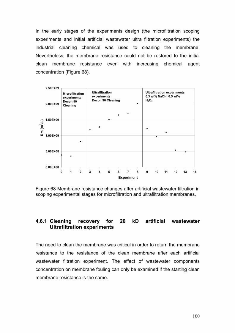
100

In the early stages of the experiments design (the microfiltration scoping

experiments and initial artificial wastewater ultra filtration experiments) the

industrial cleaning chemical was used to cleaning the membrane.

Nevertheless, the membrane resistance could not be restored to the initial

clean membrane resistance even with increasing chemical agent

concentration (Figure 68).

0.00E+00

5.00E+08

1.00E+09

1.50E+09

2.00E+09

2.50E+09

0 1 2 3 4 5 6 7 8 9 10 11 12 13 14

Experiment

Rm

(m

2 /L)

MicrofiltrationexperimentsDecon 90 Cleaning

Ultrafiltration experimentsDecon 90 Cleaning

Ultrafiltration experiments0.3 wt% NaOH, 0.5 wt% H2O2

Figure 68 Membrane resistance changes after artificial wastewater filtration in scoping experimental stages for microfiltration and ultrafiltration membranes.

4.6.1 Cleaning recovery for 20 kD artificial wastewater Ultrafiltration experiments

The need to clean the membrane was critical in order to return the membrane

resistance to the resistance of the clean membrane after each artificial

wastewater filtration experiment. The effect of wastewater components

concentration on membrane fouling can only be examined if the starting clean

membrane resistance is the same.

101

In order to effectively clean the membrane cleaning solution was prepared in

the lab adapting the chemicals cleaning mixture used by Gan et al (1999). A

mixture made from 0.1-0.3 wt% NaOH, 0.7-0.1 wt% H2O2 and 0-50 ml Decon

90 in Millipore ultrapure water (Table 34).

Table 34 Artificial wastewater 20 kD ultrafiltration membrane cleaning results. Run

NaOH

(g) H2O2 (ml)

Deacon 90 (ml)

Temperature °C

Time (min)

Recovery (%)

F0 60 100 0 50 165.00 114 F1 50 150 50 50 90.00 108 F2 50 150 50 50 90.00 141 F3 50 150 0 50 80.00 103 F4 50 100 0 50 90.00 90 F5 43 150 25 50 90.00 109 F6 40 150 20 50 90.00 74 F7 40 150 20 50 150.00 97 F8 50 150 10 50 105.00 98 F9 50 150 10 50 90.00 102

F10 50 150 10 30 105.00 99 F11 50 100 10 30 90.00 98 F12 50 100 10 40 90.00 89 F13 50 150 10 40 100.00 106 F14 50 100 10 50 120.00 101 F15 50 150 10 50 120.00 106

The effect of the changes in the concentration of the cleaning solution

chemical component cleaning temperature and time has been examined. The

most noticeable effect is the change of sodium hydroxide concentration in the

cleaning mixture. In general increasing the concentration of sodium hydroxide

increased fouled membrane recovery (Figure 69).

Gan et al (1999) suggested that hydrolysis of polysaccharides and proteins at

high pH played a very important part in the cleaning process, with the

chemical reactions being:

Hydrolysis of polysaccharides:

612625106 OHnCOnHOHC OHn

Hydrolysis of proteins:

102

RCHORNHOHRCRNH OOHO

22

NaOH (g)

35 40 45 50 55 60 65

Re

cove

ry (

%)

70

80

90

100

110

120

130

Figure 69 Effect of increasing NaOH concentration on 20 kD membrane recovery (line is for guidance).

The changes in hydrogen peroxide concentration did not have noticeable

effect on the 5 kD membrane recovery. The average recovery for experiments

cleaned with 100 ml hydrogen peroxide was almost the same as the average

recovery for experiments cleaned with 150 ml hydrogen peroxide (

Figure 70).

Increasing the concentration of Decon 90 in the cleaning solution increased

the average membrane recovery. On average the recovery obtained for

experiments cleaned with 50 ml of Decon 90 was higher than experiments

cleaned with lower amount of Decon 90 or no Decon 90 (Figure 71).

Changing the cleaning solution temperature between 30 to 50 °C did not have

a strong effect on the membrane average recovery, although, higher

103

temperature cleaning resulted in better membrane recovery than low

temperature cleaning (Figure 72).

Longer cleaning time gave a better membrane recovery on average than

shorter cleaning time (Figure 73).

The best membrane cleaning result was obtained with increasing sodium

hydroxide and Decon 90 concentration in the cleaning solution. Hydrogen

peroxide, temperature, and time did not have a very strong effect on the

membrane recovery.

Hydrogen peroxide (ml)

90 100 110 120 130 140 150 160

Rec

ove

ry (

%)

70

80

90

100

110

120

130

Figure 70 Effect of increasing H2O2 concentration on 20 kD membrane

recovery (line is for guidance).

104

Decon 90 (ml)

0 10 20 30 40 50 60

Rec

ove

ry (

%)

70

80

90

100

110

120

130

Figure 71 Effect of increasing Decon 90 concentration on 20 kD membrane recovery (line is for guidance).

Temperature (°C)

25 30 35 40 45 50 55

Rec

ove

ry (

%)

70

80

90

100

110

120

130

Figure 72 Effect of cleaning mixture temperature on 20 kD membrane recovery (line is for guidance).

105

Time (min)

60 80 100 120 140 160 180

Rec

ove

ry (

%)

70

80

90

100

110

120

130

Figure 73 Effect of cleaning time on 20 kD membrane recovery (line is for guidance).

4.6.2 Cleaning recovery for 5 kD artificial wastewater Ultrafiltration experiments

The effect of changing the concentration of the cleaning solution chemicals

components such sodium hydroxide and hydrogen peroxide, the cleaning

temperature and cleaning time was examined. Decon 90 was not used in the

cleaning of the 5 kD membrane (Table 35).

The effect of sodium hydroxide on the 5 kD membrane recovery was not as

strong as its effect on the larger pore 20 kD membrane filter (Figure 74).

Increasing the concentration of NaOH increased the recovery, however the

increase was not as strong as the increase achieved by increasing the

hydrogen peroxide (Figure 75), temperature (Figure 76) and time (Figure 77).

106

Table 35 Artificial wastewater 5 kD ultrafiltration membrane cleaning results. Experiment

NaOH

(g) H2O2 (ml)

Decon 90 (ml)

Temperature (°C)

Time (min)

Recovery (%)

F0 20 20 0 45 120 104 F1 20 20 0 45 120 98 F2 20 20 0 45 110 95 F3 20 20 0 45 120 103 F4 15 15 0 45 90 98 F5 20 20 0 45 120 93 F6 20 20 0 40 105 99 F7 15 0 0 45 90 90 F8 25 50 0 50 120 107 F9 25 25 0 45 120 100 F10 20 20 0 45 120 103 F11 15 15 0 45 100 118 F12 20 20 0 50 120 103 F13 20 0.0 0 45 90 108 F14 20 0.0 0 45 90 83 F15 15 0.0 0 40 60 87

NaOH (g)

14 16 18 20 22 24 26

Rec

ove

ry (

%)

80

85

90

95

100

105

110

115

120

Figure 74 Effect of sodium hydroxide concentration on 5 kD membrane recovery.

107

Hydrogen peroxide (ml)

0 10 20 30 40 50 60

Rec

ove

ry (

%)

80

85

90

95

100

105

110

115

120

Figure 75 Effect of increasing H2O2 concentration on 5 kD membrane recovery.

Temperature (°C)

38 40 42 44 46 48 50 52

Rec

ove

ry (

%)

80

85

90

95

100

105

110

115

120

Figure 76 Effect of cleaning mixture temperature on 5 kD membrane recovery.

108

Time (min)

50 60 70 80 90 100 110 120 130

Rec

ove

ry (

%)

80

85

90

95

100

105

110

115

120

Figure 77 Effect of cleaning time on 5 kD membrane recovery.

109

5.0 MODELLING OF ULTRAFILTRATION DATA

5.1 Pore blocking model fitting of crossflow filtration

experiments

In their work, Vela et al (2009) adapted Hermia’s dead end filtration blocking

models for crossflow filtration (Table 36) by accounting for foulant removal

mechanisms. Vela et al. (2009) produced a modified general differential

equation 5.1.

nppsspCF

p JJJKdt

dJ 2 (5.1)

where Jp and Jpss are the initial flux and steady state flux, respectively, KCF is

a constant depending on membrane blocked area per unit of permeate flux,

permeate dynamic viscosity, TMP and membrane resistance. The value of the

parameter n depends on the blocking mechanism as follows: cake filtration

blocking (n = 0), intermediate (n = 1), complete blocking (n = 2) and standard

blocking (n = 3/2).

Filtration experiment data for the meat extract-calcium binary mixture using

the 5 kD membrane were fitted to the four blocking models using a Matlab®

program routine (Appendix C). Further, data fitting was preformed using

SigmaPlot® software package. The predictions of the fitted blocking models

were compared to the experimental filtration data for the central experiment

F1 and are presented in Figures 79 through 82.

The predictive accuracy of the model fitting was examined by comparing the

coefficients of determination, R2, for all the experiments (Table 37).

Apart from the standard blocking model, where the fitting accuracy was low,

with an average R2 value of 0.6436, all other blocking models had a high R2

value. The highest R2 value, and thus the best fitting model, was for the

110

intermediate blocking model with an average R2 value of 0.9914. The

complete blocking model and the cake filtration model were the second and

third best fitting models, with R2 values of 0.9769 and 0.9152, respectively

(Table 37).

Table 36. Crossflow membrane filtration blocking model Vela et al. (2009).

Blocking model

n Equation constant

Complete

2

tJKpssopssp

oCeJJJJ

KC

Intermediate

1

1

tJKopss

tJKpsso

ppssi

pssi

eJJ

eJJJ

Ki

Standard

3/2

22/11 tKJ

JJ

so

op

Ks

Cake filtration

0

oppss

pssp

psso

o

p

pssgl

JJJ

JJ

JJ

J

J

JKt

11ln

12

Kgl

5.1.1 Blocking models fitting meat extract-calcium binary mixture filtration experiments

Time (s)

0 2000 4000 6000 8000 10000 12000

Per

me

ate

Flu

x (m

/s)

0.00015

0.00020

0.00025

0.00030

0.00035

0.00040

Complete blocking modelFiltration data

Figure 78. Complete blocking model fitting for F1 meat extract-calcium binary mixture 5 kD membrane filtration experiments.

111

Time (s)

0 2000 4000 6000 8000 10000 12000

Per

mea

te F

lux

(m/s

)

0.00015

0.00020

0.00025

0.00030

0.00035

0.00040

Intermediate blocking modelFiltration data

Figure 79. Intermediate blocking model fitting for F1 meat extract-calcium binary mixture 5 kD membrane filtration experiments.

Time (s)

0 2000 4000 6000 8000 10000 12000

Per

mea

te F

lux

(m/s

)

0.00005

0.00010

0.00015

0.00020

0.00025

0.00030

0.00035

0.00040

Standard blocking modelFiltration data

Figure 80. Standard blocking model fitting for F1 meat extract-calcium binary mixture 5 kD membrane filtration experiments.

112

Time (s)

0 2000 4000 6000 8000 10000 12000

Per

me

ate

Flu

x (m

/s)

0.00015

0.00020

0.00025

0.00030

0.00035

0.00040

Filtration dataCake filtration model

Figure 81. Cake filtration model fitting for F1 meat extract-calcium binary mixture 5 kD membrane filtration experiments. Table 37. Blocking model R2 fitting values for meat extract-calcium 5 kD membrane filtration experiments. Experiment Complete

blocking Intermediate

blocking Standard blocking

Cake filtration

F0 0.9596 0.9815 0.4282 0.9798 F1 0.9926 0.9947 0.7429 0.9610 F2 0.9788 0.9931 0.7076 0.7630 F3 0.9876 0.9937 0.7680 0.9275 F4 0.9796 0.9942 0.5712 0.9448

average 0.9796 0.9914 0.6436 0.9152

5.1.2 Blocking model fitting for alginate-calcium binary mixture filtration experiments

Here, the cake filtration model was the best fitting model, with an R2 value of

0.8376. The standard blocking model gave the worst fitting, with an R2 value

of 0.0611. The intermediate and complete blocking model R2 values were

similar at 0.7885 and 0.7862, respectively (Table 38).

113

Time (s)

0 2000 4000 6000 8000 10000 12000

Flu

x (m

/s)

0.00010

0.00015

0.00020

0.00025

0.00030

0.00035

0.00040

Complete blocking modeFiltration data

Figure 82. Complete blocking model fitting for F1 alginate-calcium binary mixture 5 kD membrane filtration experiments.

Time (s)

0 2000 4000 6000 8000 10000 12000

Flu

x (m

/s)

0.00010

0.00015

0.00020

0.00025

0.00030

0.00035

0.00040


Figure 83. Intermediate blocking model fitting for F1 alginate-calcium binary mixture 5 kD membrane filtration experiments.

114

Time (s)

0 2000 4000 6000 8000 10000 12000

Flu

x (m

/s)

0.00000

0.00005

0.00010

0.00015

0.00020

0.00025

0.00030

0.00035

0.00040


Figure 84. Standard blocking model fitting for F1 alginate-calcium binary mixture 5 kD membrane filtration experiments.

Time (s)

0 2000 4000 6000 8000 10000 12000

Per

mea

te F

lux

(m/s

)

0.00010

0.00015

0.00020

0.00025

0.00030

0.00035

0.00040


Figure 85. Cake filtration model fitting for F1 alginate-calcium binary mixture 5 kD membrane filtration experiments.

115

Table 38. Blocking model R2 fitting values for alginate-calcium 5 kD membrane filtration experiments. Experiment Complete



Cake filtration

F0 0.9511 0.9489 0.0000 0.7831 F1 0.8982 0.8696 0.0000 0.8541 F2 0.6850 0.7480 0.2443 0.9559 F3 0.5276 0.5876 0.0000 0.7104 F4 0.8693 0.8693 0.0000 08846

average 0.7862 0.7885 0.0611 0.8376

5.1.3 Blocking model fitting for artificial wastewater mixture 5 kD membrane filtration experiments

Here, the best fitting accuracy was obtained using the intermediate and the

complete blocking models, with R2 values of 0.9430 and 0.9133, respectively

(Table 39). The cake filtration model came in third, with an R2 value of 0.8144,

whilst the worst fitting model was the standard blocking model, with an R2

value of 0.1258 (Table 39).

Time (s)

0 2000 4000 6000 8000 10000 12000

Flu

x (m

/s)

0.00010

0.00011

0.00012

0.00013

0.00014

0.00015

0.00016

0.00017

0.00018


Figure 86. Complete blocking model fitting for F1 artificial wastewater mixture 5 kD membrane filtration experiments.

116

Time (s)

0 2000 4000 6000 8000 10000 12000

Flu

x (m

/s)

0.00010

0.00011

0.00012

0.00013

0.00014

0.00015

0.00016

0.00017

0.00018


Figure 87. Intermediate blocking model fitting for F1 artificial wastewater mixture 5 kD membrane filtration experiments.

Time (s)

0 2000 4000 6000 8000 10000 12000

Flu

x (m

/s)

0.00006

0.00008

0.00010

0.00012

0.00014

0.00016

0.00018

0.00020


Figure 88. Standard blocking model fitting for F1 artificial wastewater mixture 5 kD membrane filtration experiments.

117

Time (s)

0 2000 4000 6000 8000 10000 12000 14000

Per

mea

te F

lux

(m

/s)

0.00010

0.00011

0.00012

0.00013

0.00014

0.00015

0.00016

0.00017

0.00018


Figure 89. Cake filtration model fitting for F1 artificial wastewater mixture 5 kD membrane filtration experiments. Table 39. Blocking model R2 fitting values for artificial wastewater 5 kD membrane filtration experiments. Experiment Complete



Cake filtration

F0 0.8704 0.9107 0.0554 0.6166 F1 0.9587 0.9779 0.5291 0.9859 F2 0.9612 0.9793 0.4792 0.9170 F3 0.9067 0.9355 0.0000 0.6661 F4 0.9212 0.9531 0.0000 0.9711 F5 0.9015 0.9269 0.1864 0.8356 F6 0.9106 0.9390 0.0000 0.8419 F7 0.9145 0.9345 0.0000 0.9354 F8 0.9694 0.9848 0.3269 0.7959 F9 0.9216 0.9571 0.0890 0.7953 F10 0.8531 0.8964 0.0000 0.5443 F11 0.9222 0.9475 0.0531 0.7102 F12 0.8525 0.8872 0.0000 0.9476 F13 0.9426 0.9698 0.2967 0.8926 F14 0.9117 0.9452 0.0481 0.9887 F15 0.9013 0.9377 0.0000 0.8126 F16 0.9066 0.9480 0.0752 0.5877

average 0.9133 0.9430 0.1258 0.8144

118

5.1.4 Blocking model fitting for artificial wastewater mixture 20 kD membrane filtration experiments

For the artificial wastewater crossflow experiments using the 20 kD

ultrafiltration membrane, the fitting accuracy of all models, with the exception

of the standard blocking model, were almost the same, with average R2

values of 0.8875, 0.8805 and 0.8733 for the cake filtration, intermediate and

complete blocking models, respectively (Table 40).

Time (s)

0 2000 4000 6000 8000 10000 12000

Flu

x (m

/s)

0.00005

0.00010

0.00015

0.00020

0.00025

0.00030

0.00035

0.00040

0.00045


Figure 90. Complete blocking model fitting for F1 artificial wastewater mixture 20 kD membrane filtration experiments.

Time (s)

0 2000 4000 6000 8000 10000 12000

Flu

x (m

/s)

0.00005

0.00010

0.00015

0.00020

0.00025

0.00030

0.00035

0.00040

0.00045


Figure 91. Intermediate blocking model fitting for F1 artificial wastewater mixture 20 kD membrane filtration experiments

119

Time (s)

0 2000 4000 6000 8000 10000 12000

Flu

x (m

/s)

0.0000

0.0001

0.0002

0.0003

0.0004

0.0005


Figure 92. Standard blocking model fitting for F1 artificial wastewater mixture 20 kD membrane filtration experiments.

Time (s)

0 2000 4000 6000 8000 10000 12000

Pe

rmea

te F

lux

(m/s

)

5.0e-5

1.0e-4

1.5e-4

2.0e-4

2.5e-4

3.0e-4

3.5e-4

4.0e-4

4.5e-4


Figure 93. Cake filtration model fitting for F1 artificial wastewater mixture 20 kD membrane filtration experiments.

120

Table 40. Blocking model R2 fitting values for artificial wastewater 20 kD membrane filtration experiments. Experiment Complete



Cake filtration

F0 0.9414 0.9414 0.0000 0.8896 F1 0.6206 0.6800 0.0000 0.9831 F2 0.5470 0.6106 0.0000 0.7706 F3 0.8797 0.8797 0.0000 0.8874 F4 0.9257 0.9257 0.0000 0.9035 F5 0.8912 0.8912 0.0000 0.8272 F6 0.9530 0.9530 0.0000 0.8074 F7 0.9049 0.9049 0.0000 0.8886 F8 0.9023 0.9024 0.0000 0.9510 F9 0.8753 0.8754 0.0000 0.9358 F10 0.9513 0.9513 0.0000 0.9014 F11 0.9285 0.9285 0.0000 0.8716 F12 0.9861 0.9861 0.0000 0.7859 F13 0.8947 0.8947 0.0000 0.8713 F14 0.8530 0.8531 0.0000 0.9367 F15 0.8769 0.8769 0.0000 0.9225 F16 0.9147 0.9147 0.0000 0.9538

average 0.8733 0.8806 0.0000 0.8875

5.2 Effects of artificial wastewater component concentrations

on the pore blocking model fitting accuracy

5.2.1 Artificial wastewater 5 kD membrane crossflow filtration experiments

The effects of varying the concentrations of the main four wastewater

components, peptone, meat extract, alginate and calcium, on the blocking

mechanisms was investigated in this section. Minitab software factorial design

algorithms (Appendix D) were used to analyse the effect of changing

component concentration levels on the blocking model accuracy by using the

coefficients of determination, R2, of the intermediate, complete, standard, and

cake filtration blocking models calculated using matlab® route (Appendix B) .

121

5.2.1.1 Intermediate blocking model The change in peptone concentration level had a minor, almost negligible

effect on the goodness of fit of the intermediate blocking model (Figure 95).

Changes in the meat extract concentration level had biggest effect on the

fitting of the intermediate blocking model compared to the other three

components. Increasing the meat extract concentration improved R2 from

0.932 at the low concentration level to 0.958 at the high level on average

(Figure 95). Increasing the concentration level of alginate reduced the R2 from

0.952 at the low level to 0.936 at the high level (Figure 95). Similar to the

alginate effect on the fit of the intermediate blocking model was the effect of

increasing the calcium concentration; here, the R2 was reduced from 0.957 at

the low level to 0.931 at the high level (Figure 95).

27018090

0.96

0.94

0.92

27018090

15010050

0.96

0.94

0.92

604020

Peptone

Mod

el f

itti

ng a

ccur

acy

Meat extract

Alginate CaCl2

CornerCenter

Point Type

Concentration (ppm)

Figure 94. Main effects of wastewater components on intermediate blocking model R2 values for the 5 kD ultrafiltration membrane.

The intermediate blocking model is considered to be accurate when the solute

molecules are of the same size as the membrane pores; furthermore, it

accounts for the possibility of molecules landing on top of each other rather

than on the free membrane surface (Vela et al., 2009). The fact that

122

increasing the meat extract concentration led to an improvement in the fit of

the intermediate blocking model indicated that the meat extract particles were

close in size to the membrane pore size of the 5 kD membrane. In contrast,

alginate particle size was much larger than the membrane pore size;

therefore, increasing alginate concentration had an adverse effect on the

intermediate blocking model predictions. The bridging effect of calcium

cations likely resulted in agglomeration and thus larger particle sizes for

alginate and proteins which in turn reduced the fitting accuracy of the

intermediate blocking model.

5.2.1.2 Complete blocking model The change in peptone concentration level had a small effect on the accuracy

of the complete blocking model fitting. At the high concentration of peptone

the R2 was 0.92 and at the low level it was 0.914 (Figure 96).

Changes in the meat extract concentration level had the second largest effect

on the coefficient of determination of the complete blocking model. At the low

meat extract level, the R2 value was 0.904 and at the high level the value R2

was 0.939. The higher concentration of meat extract resulted in a better fitting

of the complete blocking model (Figure 96).

Similarly to the alginate effect on the fitting of the intermediate model,

increasing the concentration of alginate reduced the goodness of fit of the

complete blocking model. At the low alginate concentration level, the R2 was

0.923 and it was 0.910 at the high level.

The largest effect on the goodness of fit of the complete blocking model

resulted from changes in calcium concentration level. The high calcium

concentration level resulted in lowering the R2 value to 0.897, compared to an

R2 value of 0.935 at the high level (Figure 96).

123

As in the intermediate blocking model, the complete blocking model assumes

that each particle arriving at the membrane surface blocks membrane pores

by sealing them; nevertheless, unlike the intermediate blocking model, where

particles can be deposited on top of each other, in the complete blocking

model particles never settle over another molecule.

Similarly to the intermediate blocking model, increasing the meat extract

concentration level increased the model fitting accuracy. Since small particle

components such as meat extract have more chances to block membrane

pores, increasing the fraction small particles, close to membrane pore size,

will lead to better fitting of the complete blocking model.

Conversely, large molecular particles such as alginate are less likely to seal

pore membrane, thus increasing the concentration of alginate had an adverse

effect on the complete blocking model goodness of fit.

Further, increasing the calcium cation concentration encourages the formation

of larger particles through ionic bonding and the alginate calcium bridging

effect.

27018090

0.94

0.92

0.90

0.88

27018090

15010050

0.94

0.92

0.90

0.88

604020

Peptone

Mod

el f

itti

ng a

ccur

acy

Meat extract

Alginate CaCl2

CornerCenter

Point Type

Concentration (ppm)

Figure 95. Main effects of wastewater components on complete blocking model R2 values for the 5 kD ultrafiltration membrane.

124

5.2.1.3 Cake filtration model Increasing the peptone concentration level reduced the accuracy of the cake

filtration model. At a low peptone concentration, the R2 value was 0.87, and at

a high level, it was 0.79 (Figure 97).

The increase in meat extract concentration reduced the accuracy of the cake

filtration model fitting. At a low meat extract concentration, the R2 value was

0.84 whilst the higher meat extract concentration level resulted in an R2 value

of 0.81 (Figure 97).

The cake filtration model fitting accuracy increased with increasing alginate

concentration. The value of R2 at the high alginate concentration level was

0.88 and at the low level it was 0.78.

The change in calcium level did not have a large effect on the cake filtration

model accuracy. The values of R2 at high and low calcium levels were 0.84

and 0.81, respectively (Figure 97).

27018090

0.85

0.80

0.75

0.70

0.65

27018090

15010050

0.85

0.80

0.75

0.70

0.65

604020

Peptone

Mod

el f

itti

ng a

ccur

acy

Meat extract

Alginate CaCl2

CornerCenter

Point Type

Concentration (ppm) Figure 96. Main effects of wastewater components on cake–filtration model R2 values for the 5 kD ultrafiltration membrane.

125

The cake filtration model assumes that the particles are larger than the

membrane pores thus they do not enter the membrane pore; rather, particles

form a cake layer on top of the membrane. Since peptone and meat extract

molecules are not too large compared to the membrane pore size, increasing

the concentration of these components reduced the fitting accuracy of the

model. In contrast, increasing the concentration level of large molecules such

as alginate increased the predictive accuracy of the cake filtration model.

Although increasing the concentration of calcium should ideally increase the

accuracy of the cake filtration model by reducing the fraction of small particles

via ionic bonding and the alginate calcium bridging effect, there was only a

small effect resulting from increasing the calcium concentration.

5.2.1.4 Standard blocking model For the standard blocking model, the fitting accuracy did not change

noticeably with the change of component concentrations. The value of R2 was

very low for this model; the maximum R2 value obtained was 0.2 at the high

concentration level of meat extract and the low level of calcium chloride, whilst

the change in peptone and sodium alginate concentration levels had no effect

on the accuracy of the standard blocking model (Figure 98).

27018090

0.20

0.15

0.10

0.05

0.0027018090

15010050

0.20

0.15

0.10

0.05

0.00604020

Peptone

Mod

el f

itti

ng a

ccur

acy

Meat extract

Alginate CaCl2

CornerCenter

Point Type

Concentration (ppm) Figure 97. Main effects of wastewater components on standard blocking model R2 values for the 5 kD ultrafiltration membrane.

126

5.2.2 Artificial wastewater 20 kD membrane crossflow filtration experiments

5.2.2.1 Intermediate blocking model

The change in peptone concentration had an effect on the accuracy of the

intermediate blocking model fitting. The higher peptone concentration resulted

in reducing the R2 value to 0.879 from a value of 0.915 at the lower peptone

level (Figure 99).

Changes in the meat extract concentration had a similar effect as peptone

levels on the accuracy of the intermediate blocking model fitting. The R2 value

at the low meat extract level was higher, at 0.910, than its value at the high

level, which was 0.875 (Figure 99).

The high alginate level resulted in a lower R2 value for the intermediate

blocking model than for the low level. The R2 value was 0.90 at the low

alginate level and 0.88 at the high alginate level (Figure 99).

The change in calcium concentration level had the greatest effect on the

accuracy of the intermediate blocking model. The higher concentration of

calcium resulted in a better fitting accuracy. The value of R2 at the low calcium

level was 0.865, which was lower than the value of R2 at the high level, 0.915

(Figure 99).

Unlike the case with the 5 kD membrane, increasing the concentration level of

peptone and meat extract did not improve the accuracy of the intermediate–

blocking model prediction. Moreover, the improvement of the model prediction

with increased calcium concentration may suggest that peptone and meat

extract particles are much smaller than the 20 kD membrane pore size and

that the bonding effect of the calcium cations brings these agglomerated

127

particles closer to the membrane size, thus increasing the intermediate

blocking mechanisms.

27018090

0.94

0.92

0.90

0.88

0.8627018090

15010050

0.94

0.92

0.90

0.88

0.86604020

Peptone

Mod

el f

itti

ng a

ccur

acy

Meat extract

Alginate Calcium

CornerCenter

Point Type

Concentration (ppm)

Figure 98. Main effects of wastewater components on intermediate blocking model R2 values for the 20 kD ultrafiltration membrane.

5.2.2.2 Complete blocking model

Changes in peptone concentration had an effect on the accuracy of the

complete blocking model fitting. The higher peptone concentration resulted in

lowering the R2 value to 0.865 from a value of 0.906 at the low peptone level

(Figure 100).

Changes in the meat extract concentration had a similar effect on the

accuracy of the complete blocking model fitting as for peptone. The value of

R2 at the low meat extract concentration level was higher, at 0.906, than its

value at the high level, which was 0.863 (Figure 100).

128

The high alginate concentration level resulted in a lower R2 value for the

complete blocking model than low level; R2 was 0.907 at low alginate

concentration and 0.863 at high concentration (Figure 100).

The change in calcium concentration level had the greatest effect on the

accuracy of the complete blocking model among all the components. The

higher concentration of calcium resulted in a better fitting accuracy. The value

of R2 at the low calcium level was 0.856 but increased to 0.925 at the high

level (Figure 100).

As with the intermediate blocking model, and unlike the case with the 5 kD

membrane, increasing the concentration level of peptone and meat extract did

not improve the accuracy of the complete blocking model predictions.

Furthermore, the effect of increased calcium concentration in improving the

model prediction suggests that peptone and meat extract particles are much

smaller than the 20 kD membrane pore size and that the bonding effect of the

calcium cations brings the agglomerated particles closer to the membrane

size, thus increasing the influence of the complete blocking mechanism.

27018090

0.950

0.925

0.900

0.875

0.85027018090

15010050

0.950

0.925

0.900

0.875

0.850604020

Peptone

Mod

el f

itti

ng a

ccur

acy

Meat extract

Alginate Calcium

CornerCenter

Point Type

Concentration (ppm)

Figure 99. Main effects of wastewater components on complete blocking model R2 values for the 20 kD ultrafiltration membrane.

129

5.2.2.3 Cake filtration model

The change in peptone concentration level affected the fitting accuracy of the

cake filtration model. The lower concentration level of peptone improved the

accuracy of the cake filtration model compared to the higher level. The value

of R2 at the low level was 0.91 and was 0.865 at the high level (Figure 101).

The higher meat extract concentration level resulted in a higher accuracy of

prediction for the cake filtration model than lower level. The value of R2 at the

low level was 0.865 and it was 0.910 at the high level (Figure 101).

The lower concentration level of alginate yielded a better cake filtration model

fitting than the higher level. The R2 value at the low level was 0.915, which is

much higher than its value at the high level, of 0.86 (Figure 101).

Changing the calcium concentration level had a marginal effect on the

accuracy of the cake filtration model. The R2 value at the low level was 0.88

compared to 0.89 at the high level (Figure 101).

27018090

0.92

0.90

0.88

0.86

27018090

15010050

0.92

0.90

0.88

0.86

604020

Peptone

Mod

el f

itti

ng a

ccur

acy

Meat extract

Alginate Calcium

CornerCenter

Point Type

Concentration (ppm)

Figure 100. Main effects of wastewater components on cake filtration blocking model R2 values for the 20 kD ultrafiltration membrane.

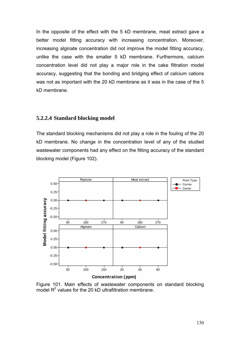
130

In the opposite of the effect with the 5 kD membrane, meat extract gave a

better model fitting accuracy with increasing concentration. Moreover,

increasing alginate concentration did not improve the model fitting accuracy,

unlike the case with the smaller 5 kD membrane. Furthermore, calcium

concentration level did not play a major role in the cake filtration model

accuracy, suggesting that the bonding and bridging effect of calcium cations

was not as important with the 20 kD membrane as it was in the case of the 5

kD membrane.

5.2.2.4 Standard blocking model

The standard blocking mechanisms did not play a role in the fouling of the 20

kD membrane. No change in the concentration level of any of the studied

wastewater components had any effect on the fitting accuracy of the standard

blocking model (Figure 102).

27018090

0.50

0.25

0.00

-0.25

-0.50

27018090

15010050

0.50

0.25

0.00

-0.25

-0.50

604020

Peptone

Mod

el f

itti

ng a

ccur

acy

Meat extract

Alginate Calcium

CornerCenter

Point Type

Concentration (ppm)

Figure 101. Main effects of wastewater components on standard blocking model R2 values for the 20 kD ultrafiltration membrane.

131

5.2.3 Meat extract-calcium binary mixture crossflow filtration experiments


Changing the concentration level of meat extract did not have a noticeable

effect on the fitting accuracy of the intermediate blocking model. The R2 value

at the low concentration level was 0.994 and it was 0.993 at the high level.

Changing the concentration level of calcium also had no effect on the

accuracy of the intermediate blocking model (Figure 103).

27018090

0.994

0.992

0.990

0.988

0.986

0.984

0.982

0.980604020

Meat extract

Mod

el f

itti

ng a

ccur

acy

CalciumCornerCenter

Point Type

Concentration (ppm)

Figure 102. Main effects of meat extract-calcium binary mixture components on intermediate blocking model R2 values for 5 kD membrane filtration.


Changing the concentration level of meat extract did not have a noticeable

effect on the fitting accuracy of the complete blocking model. The R2 value at

low meat extract concentration level was 0.990 and its value at the high level

was 0.980 (Figure 104).

The change in calcium concentration level also had no effect on the fitting

accuracy of the complete blocking model. The values of R2 for the high and

132

low concentrations of calcium were 0.983 and 0.985, respectively (Figure

104).

27018090

0.990

0.985

0.980

0.975

0.970

0.965

0.960

604020

Meat extract

Mod

el f

itti

ng a

ccur

acy

CalciumCornerCenter

Point Type

Concentration (ppm) Figure 103. Main effects of meat extract-calcium binary mixture components on complete blocking model R2 values for 5 kD membrane filtration.


Changing the concentration level of meat extract had a large effect on the

fitting accuracy of the cake filtration model. The value of R2 at low meat

extract concentration was 0.944 while the value of R2 at high meat extract

concentration was 0.854 (Figure 105).

27018090

0.975

0.950

0.925

0.900

0.875

0.850604020

Meat extract

Mod

el f

itti

ng a

ccur

acy

CalciumCornerCenter

Point Type

Concentration (ppm)

Figure 104. Main effects of meat extract-calcium binary mixture components on cake filtration blocking model R2 values for 5 kD membrane filtration.

133

Increasing the calcium concentration improved the cake filtration model fitting

accuracy. The R2 value at the low calcium concentration level was 0.86 while

it was 0.938 at the high level (Figure 105).


Changing the meat extract concentration had a minor effect on the accuracy

of the standard blocking model. The values of R2 were 0.75 at the low meat

extract concentration level and 0.65 at the high level (Figure 106).

27018090

0.8

0.7

0.6

0.5

0.4604020

Meat extract

Mod

el f

itti

ng a

ccur

acy

CalciumCornerCenter

Point Type

Concentration (ppm)

Figure 105. Main effects of meat extract calcium binary mixture components on standard blocking model R2 values for 5 kD membrane filtration.

Changing calcium concentration level had a minor effect on the fitting

accuracy of the standard blocking model. The R2 value for the low and high

concentration levels of calcium were 0.725 and 0.675, respectively (Figure

106). Compared to the other models, the standard model had the lowest fitting

accuracy.

134

5.2.4 Sodium alginate-calcium binary mixture cross-flow filtration experiments


The change in the concentration of alginate had an effect on the fitting

accuracy of the intermediate blocking model. Lowering the alginate

concentration level improved the accuracy of the intermediate blocking model.

The R2 value at the low concentration level was 0.863, while the R2 value at

the high level was 0.725 (Figure 107).

Changing the calcium concentration had a large effect on the fitting accuracy

of the intermediate blocking model. Increasing the concentration lowered the

R2 value from 0.92 at the low concentration level to 0.62 at the high level

(Figure 107).

15010050

0.95

0.90

0.85

0.80

0.75

0.70

604020

Sodium Alginate

Mod

el f

itti

ng a

ccur

acy

CalciumCornerCenter

Point Type

Concentration (ppm) Figure 106. Main effects of alginate-calcium binary mixture components on intermediate blocking model R2 values for 5 kD membrane filtration.

135


Increasing the alginate concentration had an adverse effect on the fitting

accuracy of the complete blocking model, lowering the R2 value from 0.83 at

the low concentration level to 0.71 at the high level (Figure 108).

The change in the calcium concentration level had the largest effect on the

fitting accuracy of the complete blocking model. The value of R2 at the low

concentration level of calcium was 0.94, while it was 0.61 at the high level

(Figure 108).

15010050

0.95

0.90

0.85

0.80

0.75

0.70

0.65

0.60

604020

Sodium Alginate

Mod

el f

itti

ng a

ccur

acy

CalciumCornerCenter

Point Type

Concentration (ppm)

Figure 107. Main effects of alginate-calcium binary mixture components on complete blocking model R2 values for 5 kD membrane filtration.


The change in the concentration level of alginate had an effect on the fitting

accuracy of the cake filtration model. Increasing the concentration of alginate

lowered the R2 value from 0.87 at the low concentration level to 0.78 at the

high level (Figure 109).

136

Increasing the concentration level of calcium marginally improved the fitting

accuracy. The values of R2 were 0.82 at the low concentration level and 0.83

at the high level (Figure 109).

15010050

0.88

0.86

0.84

0.82

0.80

0.78

604020

Sodium Alginate

Mod

el f

itti

ng a

ccur

acy

CalciumCornerCenter

Point Type

Concentration (ppm) Figure 108. Main effects of alginate-calcium binary mixture components on cake filtration blocking model R2 values for 5 kD membrane filtration.


The fitting accuracy of the standard blocking model was very low. Changing

the concentrations of alginate or calcium did not have a noticeable effect on

the fitting accuracy of the standard blocking model (Figure 110).

137

15010050

0.12

0.10

0.08

0.06

0.04

0.02

0.00

604020

Sodium Alginate

Mod

el f

itti

ng a

ccur

acy

CalciumCornerCenter

Point Type

Concentration (ppm) Figure 109. Main effects of alginate-calcium binary mixture components on standard blocking model R2 values for 5 kD membrane filtration.

5.3 Concentration polarisation model

The assumption of uniform non-interacting particles in the feed is a major

shortfall in this theory due to the well established concept of interaction

between cations and several wastewater components such as proteins and

polysaccharides, as well as the self interaction of wastewater components.

A second assumption that maybe a source of error in the model predictions

for flux is 100% particle rejection by the membrane, which is unrealistic, as

real wastewater contains many components with particle sizes smaller than

the pores of the membrane, and certainly a microfiltration membrane, so the

flux will be theoretically reduced by other blocking mechanisms such as

complete and intermediate blocking, perhaps more greatly than by the

resistance of the concentration polarisation layer.

In their theory of concentration polarisation, Song and Elimelech (1995)

introduced the filtration number, NF, a dimensionless number.

138

pp

F PkT

aN

3

4 3 (5.2)

The filtration number represents a ratio between the energy needed to move

the particle from the membrane surface back into the bulk suspension and the

particle’s thermal energy.

A critical value of 15 is assigned to the filtration number. If the filtration

number is less than the critical value, then a concentration polarisation layer

exists over the membrane surface, and if the filtration number value is larger

than the critical value a cake layer with maximum packing starts to form on

the membrane surface.

The calculation procedure is to solve equation (5.2) by substituting ∆P for ∆Pp

then solve equation (5.3) for θ, which is a porosity dependent factor.

w

dPkT

ap

p

0

2

65

53

3

2

3

2

31

3

21

3

4 (5.3)

Finally the variable )( *sA is calculated using equation (5.4) (Song and

Elimelech, 1995):

3* )(

w

Fs

NA

(5.4)

The flux when a cake layer is formed can be calculated from equation (5.5).

3/1

0max

3/13/13/23/2

)(2

3

kTCAs

PLDV

(5.5)

139

In all the artificial wastewater experiments performed in this study, the

filtration number (NF) value was larger than 15, indicating the formation of a

cake layer.

As can be seen from equation (5.2), the filtration number depends here only

on the particle size as all other variables, such as pressure and temperature,

were constant in the artificial wastewater experiments performed in this study.

The change in the steady state flux with different particle sizes for the

constant operating conditions used in the wastewater filtration experiments is

presented in (Figure 110).

0.00

200.00

400.00

600.00

800.00

1000.00

1200.00

1400.00

4.00 5.00 6.00 7.00 8.00 9.00 10.00 11.00

log (ap)

Ste

ad

y s

tate

Flu

x (

L/m

^2 h

)

Figure 110. Steady state flux vs. particle diameter for artificial wastewater experiments calculated using the Song and Elimelech concentration polarisation equation.

Although the particle size analysis by the Malvern Mastersizer failed in the

quality factor due to the high polydispersity of the wastewater feed, the results

were used to compare the concentration polarisation model predictions to the

experimental results (Table 41).

140

Table 41. Concentration polarisation model predictions for steady state flux versus experimental wastewater filtration results.

Experiment Jss (L/m2 h) Model Jss (L/m2 h) Error (%) F0 376 N/A N/A F1 475 N/A N/A F2 447 497 11 F3 551 N/A N/A F4 373 N/A N/A F5 482 491 2 F6 444 544 23 F7 452 473 5 F8 463 560 21 F9 418 449 7

F10 335 433 29 F11 427 439 3 F12 304 414 36 F13 385 478 24 F14 411 588 43 F15 440 497 13 F16 402 480 19

The model over predicted the steady state flux for all experiments. The best

prediction was for experiment F5, with a 5% error, and the worst prediction

was for experiment F14, with over 43% prediction error.

141

6.0 Conclusions and Recommendations

The microfiltration membrane could not reject the artificial wastewater

components. The permeate flux reduced with time, nevertheless, the

permeate Chemical Oxygen Demand (COD) was the same as the artificial

wastewater feed. The flux reduction indicates a blocking of membrane pores

and the permeate COD value indicates that the microfiltration pore size 0.2

µm was larger than the artificial wastewater component particles size.

Smaller pore size ultrafiltration membranes were used to carry on the

experiments in this work to better examine the effect of different artificial

wastewater components on the fouling of the ceramic membranes.

Flux analysis for 20 and 5 kD membranes showed a great influence of

calcium concentration. As calcium concentration increased the flux reduction

increased. Further, with the 5 kD membrane the largest flux reduction was

obtained with high concentration of both calcium and alginate. This is a result

of the fouling layer becoming more compacted and more resistance to

permeate flow as a result of the calcium bridging effect on alginate.

Increasing calcium concentration level had the strongest effect on increasing

membrane resistance. The average increase is membrane resistance for

experiments conducted with a high calcium concentration of 60 ppm

compared to the increase in membrane resistance for experiments conducted

with low calcium concentration of 20 ppm was 100% and 32% for the 20 and

5 kD membrane, respectively.

It is clear from the comprehensive set of results and factorial design analysis

of the artificial wastewater filtration experiments performed here that the

concentration of calcium is a very important factor that must be considered in

wastewater filtration. Furthermore, the soluble microbial products, especially

polysaccharides, are one of the main components responsible for membrane

fouling. The following can be concluded from the two level factorial design

analysis:

142

Polysaccharides are the major fouling compounds in EPS.

While protein compounds are an important part of EPS membrane

fouling, their effect increases in the presence of polysaccharides.

Sodium alginate-calcium solutions fouled the membrane more

severely, causing twice the increase of resistance (on average) than

did meat extract-calcium solutions.

Irreversible fouling was the major fouling type in alginate-calcium

filtration experiments (95% in four of the five experiments), while 30 –

40 % of the fouling in the meat extract-calcium filtration experiments

was reversible fouling.

Clear relationships between the calcium to alginate ratio and both the

extent and type of membrane fouling exist. However, when meat

extract was the main foulant, no clear relationship between fouling

level and meat extract to calcium ratio was observed.

At calcium to alginate concentration ratios between 0.05 – 0.07, free

calcium cations were found in the mixtures. At concentration ratios

equal to or less than 0.05, nearly all calcium cations were bound by

the alginate.

For the meat extract–calcium solutions, 50% of the initial feed calcium

was absorbed by the meat extract, regardless of the change in calcium

feed concentration.

Choosing the appropriate cleaning method is an important factor for improving

a membrane separation process. The cleaning chemicals and the frequency

of cleaning are both functions of the process stream components and

concentrations. Sodium hydroxide concentration in the cleaning solution was

the most important factor in the recovery of the ceramic membrane used in

artificial wastewater filtration. Further, higher cleaning temperature and longer

cleaning time generally gave an increase in membrane recovery after filtration

experiments nevertheless their effect was not as noticeable as increasing the

sodium hydroxide concentration.

143

The fitting accuracy of the intermediate and complete blocking models was

the highest for the filtration of the meat extract and calcium binary mixtures.

The alginate-calcium binary mixture was best fitted with the cake filtration

model. The artificial wastewater filtration data had the highest fitting accuracy

with the intermediate and complete blocking for the 5 kD membrane and the

cake filtration and intermediate blocking models for the 20 kD membrane.

The prediction accuracy of the complete, intermediate and standard blocking

models increased with increasing meat extract concentration. The increase in

calcium and alginate concentration lowered the prediction accuracy of

complete, intermediate and standard blocking models. On the other hand,

increases in calcium and alginate concentration had a positive effect on the

predication accuracy of the cake filtration model for the 5 kD pore size

membrane.

The effect of changing the artificial wastewater components concentration on

the fitting accuracy of the blocking models for the 20 kD pore size membrane

was almost the opposite of the 5 kD pore size membrane. Increasing the

calcium concentration increased the predication accuracy of the intermediate

and complete blocking models, while the increase in alginate concentration

reduced the cake filtration model prediction accuracy.

In the case of the relatively smaller pore size 5 kD membrane the smaller

particles size proteins blocked the pores completely or partially while large

alginate particles formed a cake layer over the membrane. However, in the

case of the relatively large size 20 kD membrane the increase in calcium

concentration increased the particles size of the artificial wastewater by the

calcium bridging effect on proteins and polysaccharides to produce a particles

size able to completely or partially block the 20 kD membrane pores.

Furthermore understanding the mechanism and the scale at which different

wastewater components effect the membrane fouling rate will help produce

better operating procedures. Moreover, accurate prediction of the fouling rate

144

will enable membrane filtration operators to optimise the cleaning procedure

and cleaning time intervals.

The blocking models compared in this study clearly indicated that complicated

blocking mechanisms were responsible for fouling the membrane. It would be

very interesting to combine several blocking mechanisms into one model to

account for the complexity associated with real wastewater filtration. Further,

a predictive model that takes into account the interaction between different

wastewater components would surely give far better predictions of permeate

flux and membrane fouling than existing models, which sometimes

oversimplify the complexity of wastewater component interactions.

145

Nomenclature aP Particle size (µm)

Cb Bulk particle concentration (mg/L)

Cip Solute concentration in permeate (mg/L)

Cir Retentate particle concentration (mg/L)

COD Chemical oxygen demand (ppm)

D Diffusion coefficient (m2/s)

IC Inorganic carbon concentration (ppm)

J Permeate flux (L/m2 hr)

Jcw Clean water permeate flux (L/m2 hr)

Jo Initial clean membrane water flux (L/m2 hr)

Jpss Steady state permeate flux (L/m2 hr)

Kgl Cake filtration model fitting parameter (s/m2)

kc complete blocking model fitting parameter (1/m)

KCF Crossflow filtration blocking models constant

ki Intermediate blocking model fitting parameter (1/m)

ks Standard blocking model fitting parameter (s-0.5 m-0.5)

L Membrane filter length (m)

NF Dimensionless filtration number

Rc Cake layer resistance (1/m)

Rcw Clean membrane resistance (1/m)

Ri Membrane rejection for specie i (%)

Rm Membrane resistance (1/m)

Rss Steady state membrane resistance (1/m)

T Absolute temperature (K)

t Time (s)

TC Total carbon concentration (ppm)

V Permeate total volume (L)

v Permeate volume per unit membrane area (m3/m2)

Xi Component i concentration level for factorial design analysis (ppm)

βi Factorial design interaction parameter

146

γ Shear rate (1/s)

ΔP Transmembrane pressure drop (Pa)

θ Porosity dependent factor (%)

θw Value of θ at the membrane surface

Κ Boltzmann constant (J/K)

μ Fluid dynamic viscosity (Pa s)

147

References

Aptel, P, 1994, "Membrane pressure driven processes in water treatment", Membrane processes in separation and purification, 263-281. Abrahamse, A.J., Lipreau, C., Li, S. and Heijman, S.G.J. 2008, "Removal of divalent cations reduces fouling of ultrafiltration membranes", Journal of Membrane Science, 323(1), 153-158. Al-Halbouni, D., Dott, W. and Hollender, J. 2009, "Occurrence and composition of extracellular lipids and polysaccharides in a full-scale membrane bioreactor", Water Research, 43, (1), 97-106. Arabi, S. and Nakhla, G. 2008, "Impact of calcium on the membrane fouling in membrane bioreactors", Journal of Membrane Science, 314(1-2), 134-142. Aspelund M.T., Rozeboom G., Heng M. and Glatz C.E., 2008, “Improving permeate flux and product transmission in the microfiltration of a bacterial cell suspension by flocculation with cationic polyelectrolytes”, Journal of Membrane Science, 324(1-2), 198-208. Baeyens, J., Hosten, L. and Van Vaerenbergh, E. 1997, Wastewater treatment, Kluwer Academic Publishers, The Netherlands. Bin, Z., Baosheng, S., Min, J., Taishi, G. and Zhenghong, G. 2008, "Extraction and analysis of extracellular polymeric substances in membrane fouling in submerged MBR", Desalination, 227(1-3), 286-294. Bodzek, M., Waniek, A. and Konieczny, K. 2002, "Pressure driven membrane techniques in the treatment of water containing THMs", Desalination, 147(1-3), 101-107. Bolton, G., LaCasse, D. and Kuriyel, R., 2006, “Combined models of membrane fouling: Development and application to microfiltration and ultrafiltration of biological fluids”, Journal of Membrane Science, 277, 75-84 Bowen, W.R., Calvo, J.I., and Hernández, A., 1995, "Steps of membrane blocking in flux decline during protein microfiltration", Journal of Membrane Science, 101(1-2), 153-165. Brindle, K., and Stephenson, T., 1996. ‘‘The application of membrane biological reactors for the treatment of wastewaters.’’ Biotechnol. Bioeng., 49, 601–610. Bruus J.H., Nielsen P.H. and Keiding K., 1992, On the stability of activated sludge flocs with implications to dewatering, Water Research, 26(12), 1597-1604.

148

Chang, I.S., Le Clech, P., Jefferson, B. and Judd, S. 2002, "Membrane fouling in membrane bioreactors for wastewater treatment", Journal of Environmental Engineering, 128, 1018. Chua, H.C., Arnot, T.C., and Howell, J.A., 2002, “Controlling fouling in membrane bioreactors operated with a variable throughput”, Desalination, 149, 225–229. Costa, A.R., de Pinho, M.N. and Elimelech, M. 2006, "Mechanisms of colloidal natural organic matter fouling in ultrafiltration", Journal of Membrane Science, 281(1-2), 716-725. Coulson, J.M., Richardson, J.F., Backhurst, J.R. and Harker, J.H., 1991, “Coulson & Richardson’s Chemical Engineering Volume 2: Particle Technology and Separation Processes”, Butterworth-Heinemann, Oxford, 869-876. Draget, K.I., Smidsrød, O. and Skjåk-Bræk, G. 2002, "Alginates from algae", Biopolymers, 6, 215–240. Evenblij, H., Geilvoet, S., Van der Graaf, J. and Van der Roest, H. 2005, "Filtration characterisation for assessing MBR performance: three cases compared", Desalination, 178(1-3), 115-124. Faibish, R.S. and Cohen, Y., 2001, “Fouling-resistant ceramic-supported polymer membranes for ultrafiltration of oil-in-water microemulsions”, Journal of Membrane Science., 185, 129–143. Fane, A.G., Fell, C.J.D. and and Nor, M.T. 1981, "Ultrafiltration/ Activated sludge system---development of a predictive model", Polymer Science Technology, 13, 631-658. Field, R.W., Wu, D., Howell, J.A., and Gupta, B.B., 1995, "Critical flux concept for microfiltration fouling", Journal of Membrane Science, 100(3), 259-272. Forster, C.F. 1971, "Activated sludge surfaces in relation to the sludge volume index", Water Research, 5(10). Frølund, B., Palmgren, R., Keiding, K. and Nielsen, P.H. 1996, "Extraction of extracellular polymers from activated sludge using a cation exchange resin", Water Research, 30(8), 1749-1758. Gan, Q., Howell, J.A., Field, R.W., England, R., Bird, M.R., and McKechinie, M.T., 1999, "Synergetic cleaning procedure for a ceramic membrane fouled by beer microfiltration", Journal of Membrane Science, 155(2), 277-289. Güell, C., Czekaj, P. and Davis, R. 1999, "Microfiltration of protein mixtures and the effects of yeast on membrane fouling", Journal of Membrane Science, 155(1), 113-122.

149

Hermia, J. 1982, "Constant Pressure Blocking Filtration Laws-Application to Power-Law Non-Newtonian Fluids", Chemical Engineering Research and Design, 60(a), 183-187. Ho, W.S.W. and Sirkar, K.K.S. (ed.) 1992, Membrane Handbook, Van Nostrand Reinhold, New York, New York. Hong, S. and Elimelech, M. 1997, "Chemical and physical aspects of natural organic matter (NOM) fouling of nanofiltration membranes", Journal of Membrane Science, 132(2), 159-181. Horan, N. and Eccles, C. 1986, "Purification and Characterization of Extracellular Polysaccharide from Activated Sludges", Water Research WATRAG, 20(11), 1427-1432. Houghton, J., Quarmby, J. and Stephenson, T. 2001, "Municipal wastewater sludge dewaterability and the presence of microbial extracellular polymer", Water Science and Technology, 44(2), 373-379. Hwang, K. J. and Lin, T. T., 2002, “Effect of morphology of polymeric membrane on the performance of cross-flow microfiltration”, Journal of Membrane Science, 199, 41-52. Jarusutthirak, C., Amy, G. and Croué, J.P. 2002, "Fouling characteristics of wastewater effluent organic matter (EfOM) isolates on NF and UF membranes", Desalination, 145(1-3), 247-255. Jermann, D., Pronk, W., Meylan, S. and Boller, M. 2007, "Interplay of different NOM fouling mechanisms during ultrafiltration for drinking water production", Water Research, 41(8), 1713-1722. Jiraratananon, R., Uttapap, D. and Sampranpiboon, P., 1998, "Crossflow microfiltration of a colloidal suspension with the presence of macromolecules", Journal of Membrane Science, 140(1), 57-66. Judd, S. and Jefferson, B. 2003, Membranes for industrial wastewater recovery and re-use, Elsevier, Oxford. Katsoufidou, K., Yiantsios, S.G. and Karabelas, A.J. 2007, "Experimental study of ultrafiltration membrane fouling by sodium alginate and flux recovery by backwashing", Journal of Membrane Science, 300(1-2), 137-146. Kim, I.S. and Jang, N. 2006, "The effect of calcium on the membrane biofouling in the membrane bioreactor (MBR)", Water Research, 40(14), 2756-2764. Kimura, K., Yamato, N., Yamamura, H. and Watanabe, Y. 2005, "Membrane fouling in pilot-scale membrane bioreactors (MBRs) treating municipal wastewater", Environmental Science & Technology, 39(16), 6293-6299.

150

Lesjean, B., Rosenberger, S., Laabs, C., Jekel, M., Gnirss, R. and Amy, G. 2005, "Correlation between membrane fouling and soluble/colloidal organic substances in membrane bioreactors for municipal wastewater treatment.", Water Science and Technology, 51(6/7), 1-8. Li, X., Gao, F., Hua, Z., Du, G. and Chen, J. 2005, "Treatment of synthetic wastewater by a novel MBR with granular sludge developed for controlling membrane fouling", Separation and Purification Technology, 46(1-2), 19-25. Li, Q. and Elimelech, M. 2004, "Organic Fouling and Chemical Cleaning of Nanofiltration Membranes: Measurements and Mechanisms", Environmental science and technology, 38(17), 4683-4693. Lu, S. G., Imai, T., Ukita, M., Sekine, M., Higuchi, T. and Fukagawa, M., 2001, “A Model for Membrane Bioreactor Process Based on the Concept of Formation and Degradation of Soluble Microbial Products”, Water Research, 35(8), 2038-2048 Lubbecke, S., Vogelpohl, A., and Dewjanin, W., 1995, ‘‘Wastewater treatment in a biological high-performance system with high biomass concentration.’’ Water Research., 29, 793–802. Mohammadi, T., Kazemimoghadam, M. and Saadabadi, M., 2003, "Modeling of membrane fouling and flux decline in reverse osmosis during separation of oil in water emulsions", Desalination,157(1-3), 369-375. Negaresh, E., Le-Clech, P. and Chen, V. 2007, "Fouling mechanisms of model polymeric substances", Asia-Pacific Journal of Chemical Engineering, 2(5), 394-399. Neyens, E., Baeyens, J., Dewil, R. and De heyder, B. 2004, "Advanced sludge treatment affects extracellular polymeric substances to improve activated sludge dewatering", Journal of Hazardous Materials, 106(2-3), 83-92. Nguyen, T.P., Hankins, N.P. and Hilal, N. 2007, "Effect of chemical composition on the flocculation dynamics of latex-based synthetic activated sludge", Journal of Hazardous Materials, 139(2), 265-274. Nguyen, T.P., Hilal, N., Hankins, N.P. and Novak, J.T., 2008a, “The relationship between cation ions and polysaccharide on the floc formation of synthetic and activated sludge”, Desalination, 227(1-3), 94-102. Nguyen, T.P., Hilal, N., Hankins, N.P. and Novak, J.T. 2008b, "Determination of the effect of cations and cationic polyelectrolytes on the characteristics and final properties of synthetic and activated sludge", Desalination, 222(1-3), 307-317.

151

Örmeci, B. and Vesilind, P.A., 2000, “Development of an improved synthetic sludge: a possible surrogate for studying activated sludge dewatering characteristics”, Water Research, 34(4), 1069-1078.

Osmonics Inc., 2002. The Osmonics Filtration Spectrum

Availble at:http://www.liquidfiltration-products.com/LiquidFiltration/Osmonicsfiltraspec.html

Palintest Ltd, 2007, Palintest Photometer 7100 Manual, Palintest Instruments, UK Prádanos, P., Hernández, A., Calvo, J.I., and Tejerina, F., 1996, "Mechanisms of protein fouling in cross-flow UF through an asymmetric inorganic membrane", Journal of Membrane Science, 114(1), 115-126. Rosenberger, S., Evenblij, H., te Poele, S., Wintgens, T. and Laabs, C. 2005, "The importance of liquid phase analyses to understand fouling in membrane assisted activated sludge processes—six case studies of different European research groups", Journal of Membrane Science, 263(1-2), 113-126. Rosenberger, S. and Kraume, M. 2003, "Filterability of activated sludge in membrane bioreactors", Desalination, 151(2), 195-200. Sanin, F.D. and Vesilind, P.A., 1999, “A comparison of physical properties of synthetic sludge with activated sludge”, Water Environment Research, 71(2), 191-196. Schäfer, A.I., Fane, A.G. and Waite, T.D. 1998, "Nanofiltration of natural organic matter: Removal, fouling and the influence of multivalent ions", Desalination, 118(1-3), 109-122. Shimizu, Y., Shimodera, K. I., and Watanabe, A., 1993, “Cross flow microfiltration of bacterial cells”J. Ferment. Bioeng., 76, 493-500 Singh, R. 2006, Hybrid membrane systems engineering for water purification : technology, systems design and operation, Elsevier, Oxford. Sobeck, D.C. and Higgins, M.J. 2002, "Examination of three theories for mechanisms of cation-induced bioflocculation", Water Research, 36(3), 527-538. Song, L. and Elimelech, M. 1995, "Theory of concentration polarization in crossflow filtration", Journal of the Chemical Society, Faraday Transactions, 91(19), 3389-3398. Song, L. 1998, "Flux decline in crossflow microfiltration and ultrafiltration: mechanisms and modeling of membrane fouling", Journal of Membrane Science, 139(2), 183-200.

152

Steiner, A., McLaren, D. and Forster, C. 1976, "The nature of activated sludge flocs", Water Research, 10(1), 25-30 Tarleton, E. and Wakeman, R. 1993, "Understanding Flux Decline in Crossflow Microfiltration-Part I-Effects of Particle and Pore Size", Chemical Engineering Research and Design, 71(a), 399-410. Tarnacki, K., Lyko, S., Wintgens, T., Melin, T. and Natau, F. 2005, "Impact of extra-cellular polymeric substances on the filterability of activated sludge in membrane bioreactors for landfill leachate treatment", Desalination, 179(1-3), 181-190. van de Ven, W.J.C., Sant, K.v., Pünt, I.G.M., Zwijnenburg, A., Kemperman, A.J.B., van der Meer, W.G.J. and Wessling, M. 2008, "Hollow fiber dead end ultrafiltration: Influence of ionic environment on filtration of alginates", Journal of Membrane Science, 308(1-2), 218-229. Varian Australia Pty. Ltd., 1989, SpectrAA 200 Manual, Australia Vela, V., Cinta, M. and Blanco, Á., 2009, "Analysis of membrane pore blocking models adapted to crossflow ultrafiltration in the ultrafiltration of PEG", Chemical Engineering Journal, 149(1-3), 232-241. Water Environment Federation 2005, Membrane systems for wastewater treatment, McGraw-Hill, London. Yamamoto, K., issa, M., Mahmood, T., and Matsuo, T., 1989, “Direct solid liquid separation using hollow fiber membrane in an activated sludge aeration tank” Water Science and Technology, 21, 43-54. Ye, Y., Clech, P.L., Chen, V. and Fane, A. 2005a, "Evolution of fouling during crossflow filtration of model EPS solutions", Journal of Membrane Science, 264(1-2), 190-199. Ye, Y., Le Clech, P., Chen, V., Fane, A.G. and Jefferson, B. 2005b, "Fouling mechanisms of alginate solutions as model extracellular polymeric substances", Desalination, 175(1), 7-20. Yoon, S., Lee, C., Kim, K. and Fane, A.G. 1998, "Effect of calcium ion on the fouling of nanofilter by humic acid in drinking water production", Water Research, 32(7), 2180-2186. Zhong, Z., Xing, W., Liu, X., Jin, W. and Xu, N., 2007, "Fouling and regeneration of ceramic membranes used in recovering titanium silicalite-1 catalysts", Journal of Membrane Science, 301(1-2), 67-75. Zhou, J., Yang, F., Meng, F., An, P. and Wang, D., 2007, "Comparison of membrane fouling during short-term filtration of aerobic granular sludge and activated sludge", Journal of Environmental Sciences, 19(11), 1281-1286.

153

Appendix A: Artificial Wastewater Experimental Results The artificial wastewater experiments filtration result for 20 kD membrane

0.00

200.00

400.00

600.00

800.00

1000.00

1200.00

1400.00

1600.00

0 2000 4000 6000 8000 10000 12000

Time (s)

Flu

x (L

/m2 h

)

Flux vs. time for experiment F0

0.00

200.00

400.00

600.00

800.00

1000.00

1200.00

1400.00

0 2000 4000 6000 8000 10000 12000

Time (s)

Flu

x (L

/m2 h

)

Flux vs. time plot for experiment F1

0.00

200.00

400.00

600.00

800.00

1000.00

1200.00

1400.00

0 2000 4000 6000 8000 10000 12000

Time (s)

Flu

x (L

/m2 h

)


154

0.00

200.00

400.00

600.00

800.00

1000.00

1200.00

1400.00

1600.00

1800.00

0 2000 4000 6000 8000 10000 12000

Time (s)

Flu

x (L

/m2 h

)


0.00

200.00

400.00

600.00

800.00

1000.00

1200.00

1400.00

1600.00

1800.00

0 2000 4000 6000 8000 10000 12000

Time (s)

Flu

x (L

/m2 h

)


0.00

200.00

400.00

600.00

800.00

1000.00

1200.00

1400.00

1600.00

0 2000 4000 6000 8000 10000 12000

Time (s)

Flu

x (L

/m2 h

)


155

0.00

200.00

400.00

600.00

800.00

1000.00

1200.00

1400.00

1600.00

1800.00

0 2000 4000 6000 8000 10000 12000

Time (s)

Flu

x (L

/m2 h

)


0.00

200.00

400.00

600.00

800.00

1000.00

1200.00

1400.00

0 2000 4000 6000 8000 10000 12000

Time (s)

Flu

x (

L/m

2 h)


0.00

200.00

400.00

600.00

800.00

1000.00

1200.00

1400.00

1600.00

1800.00

2000.00

0 2000 4000 6000 8000 10000 12000

Time (s)

Flu

x (L

/m2 h

)


156

0.00

200.00

400.00

600.00

800.00

1000.00

1200.00

1400.00

1600.00

1800.00

0 2000 4000 6000 8000 10000 12000

Time (s)

Flu

x (L

/m2 h

)


0.00

200.00

400.00

600.00

800.00

1000.00

1200.00

1400.00

1600.00

0 2000 4000 6000 8000 10000 12000

Time (s)

Flu

x (L

/m2 h

)


0.00

200.00

400.00

600.00

800.00

1000.00

1200.00

1400.00

1600.00

1800.00

0 2000 4000 6000 8000 10000 12000

Time (s)

Flu

x (L

/m2 h

)


157

0.00

200.00

400.00

600.00

800.00

1000.00

1200.00

1400.00

0 2000 4000 6000 8000 10000 12000

Time (s)

Flu

x (L

/m2 h

)


0.00

200.00

400.00

600.00

800.00

1000.00

1200.00

1400.00

1600.00

0 2000 4000 6000 8000 10000 12000

Time (s)

Flu

x (L

/m2 h

)


0.00

200.00

400.00

600.00

800.00

1000.00

1200.00

1400.00

1600.00

0 2000 4000 6000 8000 10000 12000

Time (s)

Flu

x (L

/m2 h

)


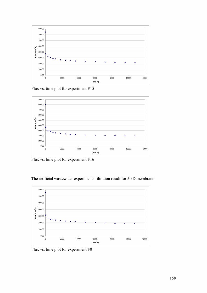
158

0.00

200.00

400.00

600.00

800.00

1000.00

1200.00

1400.00

1600.00

0 2000 4000 6000 8000 10000 12000

Time (s)

Flu

x (L

/m2 h

)


0.00

200.00

400.00

600.00

800.00

1000.00

1200.00

1400.00

1600.00

1800.00

0 2000 4000 6000 8000 10000 12000

Time (s)

Flu

x (L

/m2 h

)

Flux vs. time plot for experiment F16 The artificial wastewater experiments filtration result for 5 kD membrane

0.00

200.00

400.00

600.00

800.00

1000.00

1200.00

1400.00

0 2000 4000 6000 8000 10000 12000

Time (s)

Flu

x (L

/m2 h

)


159

0.00

200.00

400.00

600.00

800.00

1000.00

1200.00

1400.00

1600.00

0 2000 4000 6000 8000 10000 12000

Time (s)

Flu

x (L

/m2 h

)


0.00

200.00

400.00

600.00

800.00

1000.00

1200.00

1400.00

1600.00

0 2000 4000 6000 8000 10000 12000

Time (s)

Flu

x (L

/m2 h

)


0.00

200.00

400.00

600.00

800.00

1000.00

1200.00

1400.00

1600.00

0 2000 4000 6000 8000 10000 12000

Time (s)

Flu

x (L

/m2 h

)


160

0.00

200.00

400.00

600.00

800.00

1000.00

1200.00

1400.00

1600.00

0 2000 4000 6000 8000 10000 12000

Time (s)

Flu

x (L

/m2 h

)


0.00

200.00

400.00

600.00

800.00

1000.00

1200.00

1400.00

1600.00

0 2000 4000 6000 8000 10000 12000

Time (s)

Flu

x (L

/m2 h

)


0.00

200.00

400.00

600.00

800.00

1000.00

1200.00

1400.00

1600.00

0 2000 4000 6000 8000 10000 12000

Time (s)

Flu

x (L

/m2 h

)


161

0.00

200.00

400.00

600.00

800.00

1000.00

1200.00

1400.00

1600.00

0 2000 4000 6000 8000 10000 12000

Time (s)

Flu

x (L

/m2 h

)


0.00

200.00

400.00

600.00

800.00

1000.00

1200.00

1400.00

0 2000 4000 6000 8000 10000 12000

Time (s)

Flu

x (L

/m2 h

)


0.00

200.00

400.00

600.00

800.00

1000.00

1200.00

1400.00

0 2000 4000 6000 8000 10000 12000

Time (s)

Flu

x (L

/m2 h

)


162

0.00

200.00

400.00

600.00

800.00

1000.00

1200.00

1400.00

1600.00

0 2000 4000 6000 8000 10000 12000

Time (s)

Flu

x (L

/m2 h

)


0.00

200.00

400.00

600.00

800.00

1000.00

1200.00

1400.00

1600.00

0 2000 4000 6000 8000 10000 12000

Time (s)

Flu

x (L

/m2 h

)


0.00

200.00

400.00

600.00

800.00

1000.00

1200.00

1400.00

0 2000 4000 6000 8000 10000 12000

Time (s)

Flu

x (L

/m2 h

)


163

0.00

200.00

400.00

600.00

800.00

1000.00

1200.00

1400.00

0 2000 4000 6000 8000 10000 12000

Time (s)

Flu

x (L

/m2 h

)


0.00

200.00

400.00

600.00

800.00

1000.00

1200.00

1400.00

1600.00

0 2000 4000 6000 8000 10000 12000

Time (s)

Flu

x (L

/m2 h

)


0.00

200.00

400.00

600.00

800.00

1000.00

1200.00

1400.00

1600.00

1800.00

2000.00

0 2000 4000 6000 8000 10000 12000

Time (s)

Flu

x (L

/m2 h

)


164

0.00

200.00

400.00

600.00

800.00

1000.00

1200.00

1400.00

1600.00

0 2000 4000 6000 8000 10000 12000

Time (s)

Flu

x (L

/m2 h

)


165

Appendix B: The Matlab modelling programmes. The Main programme

clc clf fit_JCake; % Run the Cake filtration model fit_JComplete; % Run the Complete blocking model fit_JIntermediate; % Run the Intermediate blocking model fit_JStandard; % Run the Standard blocking model % Setup the main graph %[ax,h3]=suplabel('Blocking mechanisms fitting' ,'t'); %set(h3,'FontSize',20) % Creat a table for the fitting results table=[SSE_Cake; SSE_Complete; SSE_Intermediate; SSE_Standard]; fprintf('\n') fprintf(' Cake SSE Complete SSE Intermediate SSE Standard SSE\n') fprintf(' %2.3e %2.3e %2.3e %2.3e\n',table) fprintf('\n') table2=[Rsq_Cake; Rsq_Complete; Rsq_Intermediate; Rsq_Standard]; fprintf('\n') fprintf(' Cake Rsq Complete Rsq Intermediate Rsq Standard Rsq\n') fprintf(' %2.3f\t %2.3f\t %2.3f\t %2.3f\n',table2) fprintf('\n')

Complete blocking model fitting programme: %*******************************************************************% %Complete blocking model fitting program. %the Complet blocking model equation used in this program from the work %of Vela et al., 2009. %The program use the LSQCURVEFIT function which solves non-linear least %squares problems. %*******************************************************************% clear clf clc %loading The filtration experiment data load JMExF0.dat; %set time data to x in (s) x=JMExF0(:,1); %set permeate flux data to y in (m/s)

166

y=JMExF0(:,2); %Jo is the initial flux global Jo Jo=JMExF0(1,2); %Jpss is the steady stat flux global Jpss Jpss=JMExF0(16,2); %Initial guess %the better your initial condition guesses are, the faster %the lsqcurvefit command will converge onto a solution initialConditions = 1.0; options= optimset('TolFun',1e-20); %newParameters is an array containing the optimal values that will %generate a curve that will best fit your data %error is the sum of the error squared. the lower this number is, the better [newParameters,error] = lsqcurvefit(@JComplete, initialConditions,x,y,[],[],options); %use new parameters to get new output values y2 = JComplete(newParameters,x); %check the error diff=y-y2; diff_sq=diff.^2; SSE_Complete=sum(diff_sq); %SST and R-squired calculation y_sum=sum(y); n=numel(y); yavg=y_sum/n; diff2=y-yavg; diff2_sq=(diff2).^2; SST_Complete=sum(diff2_sq); Rsq_Complete=1-(SSE_Complete/SST_Complete); %plot the new data using the color red subplot(2,2,2) plot(x,y,'o',x,y2,'r') title('Complete blocking model fit') xlabel({'Time (s)'}) ylabel({'J (m/s)'}) hold on

Complete blocking function sub programme: function output= JComplete (param,input) global Jo % the initial flux global Jpss % the steady state flux a = param(1); % this is the Complete blocking model equation here output =Jpss + (Jo - Jpss)*exp(-a.*input.*Jo);

167

Intermediate blocking model fitting programme:

%*******************************************************************% %Intermediate blocking model fitting program. %the Intermediate blocking model equation used in this program from the work %of Vela et al., 2009. %The program use the LSQCURVEFIT function which solves non-linear least %squares problems. %*******************************************************************% clear clf clc %loading The filtration experiment data load JMExF0.dat; %set time data to x in (s) x=JMExF0(:,1); %set permeate flux data to y in (m/s) y=JMExF0(:,2); %Jo is the initial flux global Jo Jo=JMExF0(1,2); %Jpss is the steady stat flux global Jpss Jpss=JMExF0(16,2); %Initial guess %the better your initial condition guesses are, the faster %the lsqcurvefit command will converge onto a solution initialConditions = 1.0; %newParameters is an array containing the optimal values that will %generate a curve that will best fit your data options= optimset('TolFun',1e-20); %error is the sum of the error squared. the lower this number is, the better [newParameters,error] = lsqcurvefit(@JIntermediate, initialConditions,x,y,[],[],options); %use new parameters to get new output values y2 = JIntermediate(newParameters,x); % Check the error diff=y-y2; diff_sq=diff.^2; SSE_Intermediate=sum(diff_sq); % SST and Rsqr calculation y_sum=sum(y); n=numel(y);

168

yavg=y_sum/n; diff2=y-yavg; diff2_sq=(diff2).^2; SST_Intermediate=sum(diff2_sq); Rsq_Intermediate=1-(SSE_Intermediate/SST_Intermediate); %plot the new data using the color red subplot(2,2,3) plot(x,y,'o',x,y2,'r') title('Intermediate blocking model fit') xlabel({'Time (s)'}) ylabel({'J (m/s)'}) hold on

Intermediate blocking function sub programme: function output= JIntermediate (param,input) global Jo % the initial flux global Jpss % the steady state flux a = param(1); % this is the Intermediate blocking model equation here output =(Jo*Jpss*exp(Jpss*a.*input))/(Jpss + Jo*(exp(Jpss*a.*input)-1)); Standard blocking model fitting programme:

%*******************************************************************% %Standard blocking model fitting program. %the Standard blocking model equation used in this program from the work %of Vela et al., 2009. %The program use the LSQCURVEFIT function which solves non-linear least %squares problems. %*******************************************************************% clear clf clc %loading The filtration experiment data load JMExF0.dat; %set time data to x in (s) x=JMExF0(:,1); %set permeate flux data to y in (m/s) y=JMExF0(:,2); %Jo is the initial flux global Jo Jo=JMExF0(1,2); %Jpss is the steady stat flux global Jpss Jpss=JMExF0(16,2); %Initial guess %the better your initial condition guesses are, the faster

169

%the lsqcurvefit command will converge onto a solution initialConditions = 0.01; %newParameters is an array containing the optimal values that will %generate a curve that will best fit your data options= optimset('TolFun',1e-20); %error is the sum of the error squared. the lower this number is, the better [newParameters,error] = lsqcurvefit(@JStandard, initialConditions,x,y,[],[],options); %use new parameters to get new output values y2 = JStandard(newParameters,x); % Check the error diff=y-y2; diff_sq=diff.^2; SSE_Standard=sum(diff_sq); % SST ans Rsqr calculation y_sum=sum(y); n=numel(y); yavg=y_sum/n; diff2=y-yavg; diff2_sq=(diff2).^2; SST_Standard=sum(diff2_sq); Rsq_Standard=1-(SSE_Standard/SST_Standard); %plot the new data using the color red subplot(2,2,4) plot(x,y,'o',x,y2,'r') title('Standard blocking model fit') xlabel({'Time (s)'}) ylabel({'J (m/s)'}) hold on

Standard blocking function sub programme: function output= JStandard (param,input) global Jo % Initial flux global Jpss % steady state flux a = param(1); % this is the Standard blocking model equation here output =Jo./(1+Jo^2*a.*input).^2; Cake filtration model fitting programme:

%***********************************************************************% %Cake blocking model fitting program. %the Cake blocking model equation used in this program from the work %of Vela et al., 2009.

170

%The program use the LSQCURVEFIT function which solves non-linear least %squares problems. %***********************************************************************% clear clf clc %loading The filtration experiment data load JMExF0.dat; %set time data to y in (s) y=JMExF0(:,1); %set permeate flux data to x in (m/s) x=JMExF0(:,2); %Jo is the initial flux global Jo Jo=JMExF0(1,2); %Jpss is the steady stat flux global Jpss Jpss=JMExF0(16,2); %Initial guess %the better your initial condition guesses are, the faster %the lsqcurvefit command will converge onto a solution initialConditions = 10000; %newParameters is an array containing the optimal values that will %generate a curve that will best fit your data options= optimset('TolFun',1e-20); %error is the sum of the error squared. the lower this number is, the better [newParameters,error] = lsqcurvefit(@JCake, initialConditions,x,y,[],[],options); %use new parameters to get new output values y2 = JCake(newParameters,x); %Check the error diff=y-y2; diff_sq=diff.^2; SSE_Cake=sum(diff_sq); %SST and Rsqr calculation y_sum=sum(y); n=numel(y); yavg=y_sum/n; diff2=y-yavg; diff2_sq=(diff2).^2; SST_Cake=sum(diff2_sq); Rsq_Cake=1-(SSE_Cake/SST_Cake); %plot the new data using the color red subplot(2,2,1) plot(x,y,'o',x,y2,'r') title('Cake blocking model fit') xlabel({'Time (s)'}) ylabel({'J (m/s)'})

171

hold on

Cake filtration function sub programme: function output= JCake (param,input) global Jo % initial flux global Jpss % steady state flux a = param(1); % this is the Cake blocking model equation here

output = (1/(a*Jpss^2))*log(((input./Jo)*((Jo-Jpss)/(input-Jpss)))-Jpss*((1./input)-(1/Jo)));

172

Appendix C: Published Work Alazmi, R., Nassehi, V. and Wakeman, R., 2010. Calcium cation interactions with polysaccharides and proteins in wastewater UF membrane fouling. Membrane Technology, 2010(1), 6-12.

173

Appendix D: Factorial Design Calculations Numbers of factors (components) = 4 Component High Level

(mg/l) Low Level (mg/l)

Factor

Na Alginate 150 100 X1 Peptone 270 180 X2 Meat Ex. 270 180 X3 CaCl2 60 20 X4

Number of experiments needed to examine all possible combinations of high

and low factors levels are:

Number of runs = 2k , where k is the number of factors (components)

Number of runs= 24 = 16

The factorial design experimental matrix is:

Run X1 X2 X3 X4 F5 150 270 90 20 F3 50 270 90 20 F1 150 90 270 20 F8 50 90 270 20 F10 150 270 270 60 F16 50 90 270 60 F0 100 180 180 40 F15 50 270 90 60 F11 50 90 90 20 F2 150 270 270 20 F12 150 90 90 60 F9 50 270 270 60 F14 50 90 90 60 F13 50 270 270 20 F6 150 270 90 60 F7 150 90 90 20 F4 150 90 270 60

174

A response is measured (Y) in all filtration experiments such as membrane

resistance increase, permeate flux reduction, blocking model fitting

accuracy…etc.

Membrane resistance increase (Y):

Run

Y (%)

F5 225F3 195F1 293F8 185F10 313F16 278F0 263F15 328F11 227F2 313F12 231F9 243F14 285F13 300F6 263F7 264F4 320

The factorial design equation for the sixteen experiments run to be solve is:

Y = β0 + β1 X1 + β2 X2 + β3 X3 + β4 X4 +

β12 X1 X2 + β13 X1 X3 + β14 X1 X4 + β23 X2 X3 + β24 X2 X4 + β34 X3 X4 +

β123 X1 X2 X3 + β124 X1 X2 X4 + β134 X1 X3 X4 + β234 X2 X3 X4 +

β1234 X1 X2 X3 X4

where β0 is the intercept coefficient

βi is the mean effect of factor Xi

βij is the two-way interaction effect between factor Xi and Xj

βijk is the three-way interaction effect between factors Xi, Xj and Xk

βijkn is the four-way interaction effect between factors Xi , Xj , Xk and Xn

175

Minitab® Software factorial design output files Artificial wastewater 20 kD membrane crossflow experiments: ————— 09/01/2009 04:53:59 PM ———————————————————— Welcome to Minitab, press F1 for help.

Factorial Design Full Factorial Design Factors: 4 Base Design: 4, 16 Runs: 17 Replicates: 1 Blocks: none Center pts (total): 1 All terms are free from aliasing Saving file as: C:\Program Files\MTBWIN\Data\UF 20 kDa experiments.MPJ

Fractional Factorial Fit: Rss versus Peptone, Meat Ex, Alginate, CaCl2 Estimated Effects and Coefficients for Rss (coded units) Term Effect Coef Constant 268.38 Peptone -17.25 -8.63 Meat Ex 9.25 4.63 Alginate -1.00 -0.50 CaCl2 99.25 49.63 Peptone*Meat Ex 17.75 8.88 Peptone*Alginate 13.50 6.75 Peptone*CaCl2 -20.25 -10.13 Meat Ex*Alginate -27.50 -13.75 Meat Ex*CaCl2 13.75 6.88 Alginate*CaCl2 79.50 39.75 Peptone*Meat Ex*Alginate -5.50 -2.75 Peptone*Meat Ex*CaCl2 4.75 2.37 Peptone*Alginate*CaCl2 -26.50 -13.25 Meat Ex*Alginate*CaCl2 4.00 2.00 Peptone*Meat Ex*Alginate* CaCl2 25.50 12.75 Ct Pt 21.63 Analysis of Variance for Rss (coded units) Source DF Seq SS Adj SS Adj MS F P Main Effects 4 40938.8 40938.8 10234.7 * * 2-Way Interactions 6 32691.7 32691.7 5448.6 * * 3-Way Interactions 4 3084.3 3084.3 771.1 * * 4-Way Interactions 1 2601.0 2601.0 2601.0 * * Curvature 1 440.1 440.1 440.1 * * Residual Error 0 0.0 0.0 0.0 Total 16 79755.9

176

Minitab® Software factorial design output files Artificial wastewater 5 kD membrane crossflow experiments: ————— 09/01/2009 05:35:41 PM ———————————————————— Welcome to Minitab, press F1 for help. Retrieving project from file: D:\DOCUMENTS AND SETTINGS\EEZEE EEZEE\DESKTOP\MEMBRANE EXPERIMENTS\UF 5 KDA EXPERIMENTS.MPJ

Fractional Factorial Fit: Rss1 versus Peptone, Meat Ex, ... Estimated Effects and Coefficients for Rss1 (coded units) Term Effect Coef Constant 266.44 Peptone 12.12 6.06 Meat Ex 28.38 14.19 Alginate 22.63 11.31 Calcium 32.38 16.19 Peptone*Meat Ex 11.12 5.56 Peptone*Alginate -10.63 -5.31 Peptone*Calcium -3.87 -1.94 Meat Ex*Alginate 35.63 17.81 Meat Ex*Calcium -16.63 -8.31 Alginate*Calcium -24.38 -12.19 Peptone*Meat Ex*Alginate -6.13 -3.06 Peptone*Meat Ex*Calcium -40.38 -20.19 Peptone*Alginate*Calcium 14.87 7.44 Meat Ex*Alginate*Calcium 22.12 11.06 Peptone*Meat Ex*Alginate* Calcium 15.88 7.94 Ct Pt -3.44 Analysis of Variance for Rss1 (coded units) Source DF Seq SS Adj SS Adj MS F P Main Effects 4 10048.7 10048.7 2512.19 * * 2-Way Interactions 6 9565.4 9565.4 1594.23 * * 3-Way Interactions 4 9513.8 9513.8 2378.44 * * 4-Way Interactions 1 1008.1 1008.1 1008.06 * * Curvature 1 11.1 11.1 11.12 * * Residual Error 0 0.0 0.0 0.00 Total 16 30147.1

Documents

The effect of wastewater components on the fouling … · The effect of wastewater components on the fouling of ... The effect of wastewater components on the fouling of ... 2.4.3