Embed Size (px)
Citation preview
The effectiveness of quantitative easing in Japan :
New evidence from a structural factor-augmented VAR
Eric Girardin∗ and Zakaria Moussa†
September 2008
Abstract
This paper provides a new empirical framework to examine the effectiveness of Japanese
monetary policy during the "lost" decade characterized both by stagnation and deflation.
We combine advantages of Markov-Switching VAR methodology with those of structural
factor analysis in a so-called the MS-Factor-augmented VAR model to establish three major
findings. First we propose new empirical evidence supporting the ability of quantitative
easing to provide stimulation to both output and prices. Second, we show that the decisive
change in regime occurred in two steps: it crept out in May 1995 and established itself
durably in February 1999. Third, our results show that the non-neutrality of money and the
price divergence in the pre-1995 regime, which characterized the MS-VAR model, are not
present with the MS-FAVAR one.
JEL Classification : C32; E52
Keywords: Markov-switching; Factor-Augmented VAR; Japan; Monetary policy;
Transmission channels
∗Faculté de sciences Economique, Université de la Méditerrannée, 14 avenue Jules Ferry, 13621 Aix en Provence,
France, and GREQAM, 2 rue de la Charité, 13002 Marseille, France. [email protected]†Université de la Méditerranée and GREQAM, Centre de la Vieille Charité, 2 rue de la Charité, 13 002 Marseille,
France. [email protected]
1
Introduction
It is widely believed that during the "lost" decade in Japan, characterized both by stagna-
tion and deflation, monetary policy was all but impotent. Available academic work concludes
that quantitative easing, based on flooding banks with base money, did not manage to stimulate
activity or revive inflation. The conjunction between the prolonged stagnation and the deflation
that followed the financial burst in the early 1990s in Japan induced several authors to investi-
gate and to recommend different strategies to monetary authorities to get out of this situation. In
order to stop the deflationist spiral the Bank of Japan (BOJ) gradually cut the nominal interest
rates to zero. Under the non negative constraint on nominal short-term interest rates several au-
thors recommended that the BOJ should reverse sustainly private agents deflation expectations.
This would need a credible accommodation commitment and an increase of the current and fu-
ture monetary base by flooding the yen market (Krugman (2000) ; Bernanke (2000); McCallum
(2000) ; Svensson (2000) and Svensson (2003)). In March 2001 the BOJ thus decided to imple-
ment a quantitative easing monetary policy (henceforth QEMP) which consists in three pillars:
(i) to increase the monetary base by setting a quantitative target for current account balances
(CAB) at the BOJ; (ii) to make a public commitment to maintain an accommodative monetary
policy until inflation (measured by the consumer price index less perishables) registers in a sta-
ble manner a zero or positive rate; (iii) to support the quantitative objective related to current
account balances by purchasing Japan Government Bond (JGB). This policy took place until
March 2005 and since then the short-term interest rate hase been the operational target.
This paper provides a new empirical framework to examine the effectiveness of such a
strategy. By contrast to previous academic work, we find that QEMP had some effects on output
and prices. In the case of Japan, since the traditional channel of monetary policy, namely the
short-term interest rate, does not work any more, one may wonder through which transmission
channels the QEMP could affect those macroeconomic variables . Two transmission channel
for the quantitative easing policy were suggested. The first one is the expectation channel,
consisting in the " policy duration" and the "signaling effects", and the second one is the portfolio
rebalancing channel. Indeed, the commitment to maintain a zero interest rate and the expansion
of CAB at BOJ provide a signal to the private sector that the easing policy will be maintained
and induce private sector to alter its expectations about the future path of short-term interest rate
thus lowering the long-term interest rate. Beside this "policy duration effect", the increase in the
BOJ’s purchases of JGBs can be perceived as a strong signal since the central bank would bear
a great capital loss if the deflation went on. This "signaling effect" strengthens the credibility
1
of the BOJ to maintain its commitment. The second transmission mechanism is the portfolio
rebalancing channel whereby the expansion of the CABs at the BOJ and the increase in BOJ’s
purchases of JGBs would lead the private sector to alter the composition of its portfolio, lowering
yields on non-monetary assets.
When examining the transmission mechanism of monetary policy one issue which is to
be treated, particularly in the case of Japan, is the identification of instability in such a trans-
mission process. In a standard stochastic model, Orphanides and Wieland (2000) show that,
when inflation is lower than one per cent, non-linearities in the transmission process of mone-
tary policy arise solely from the presence of the zero bound on nominal interest rates. Indeed,
these effects become increasingly important for determining the outcome of monetary policy in
circumstances with such low inflation rates. On an empirical level, accounting for regime shifts
should be a major concern when examining the transmission mechanisms of monetary policy.
Our aim is to investigate the potential structural changes in transmission channels of Japanese
monetary policy on economic activity and prices. We will therefore allow for stochastic regime
switching within a vector-autoregressive model.
Among several empirical studies which evaluate the transmission channels of monetary
policy in Japan, representative recent works are Kamada and Sugo (2006), Kimura and Ugai
(2003) or Fujiwara (2006)1, many of them dealing explicitly with instability. These works admit
that examining monetary policy in a country where interest rates have come down to almost
zero, without taking into account possible structural changes would be misleading.
Kamada and Sugo (2006) adopt the VAR methodology and use the Markov Chain Monte
Carlo (MCMC) method to detect dates of possible structural changes in the Japanese econ-
omy between February 1978 and April 2005. The detected structural change point corresponds
to the peak of the asset price bubble in 1990 and results from a change in VAR parameters.
these authors show that during the post-bubble period the effect of monetary policy on prices
and production weakened. Kimura and Ugai (2003) show that transmission channel efficiency
is highly uncertain and weak. Their empirical study, based on VAR methodology with time-
varying parameters, allows them to take into account the possible changes of heterocedasticity
of money demand and of transmission mechanism when interest rates are almost zero. Even if
this methodology allows them to capture changes in economic structure and to get time-varying
impulse function responses, it does not solve the price puzzle (which characterizes VAR model)
and assumes that a single financial variable is the best indicator of the monetary policy. Fujiwara
1see Ugai (2007) for a survey
2
(2006) is the only one to use Markov-switching methods within a VAR framework (MS-VAR)
with regime-dependent impulse functions (Ehrmann et al. (2003)). The author examines the
period between 1985 and 2004 by including three and then four macroeconomic variables (in-
dustrial production, CPI, monetary base, 10 year JGB yield). This model is able to detect regime
changes without imposing a priori constraints on the time of such changes. However, this work
suffers from the non-neutrality of money and price divergence in the pre-stagnation regime.
Moreover it does not uncover any output or price effect of base money shocks during the Great
stagnation and is not able to identify in a credible way the date of regime change.
In the present paper paper MS-VAR methodology is employed following Fujiwara (2006).
However, in above quoted work only a few macroeconomic variables were taken into account
when examining the monetary policy. To conserve degrees of freedom, standard VARs rarely
employ more than six to eight variables. This matter is particularly important in the case of
a MS-VAR model when the number of estimated parameters rises very quickly. But in reality
policymakers care about an information set which contains many data series. Bernanke et al.
(2005) show that lack of information in the VAR model analysis leads to two related problems :
(i) the less the central bank and private sector related information is reflected by the analysis the
more the policy shock measure is biased. This leads to puzzles which characterize the traditional
VAR model. (ii) impulse response functions do not allow to analyze the effects of monetary
policy on general economic concepts like real economic activity or investment, which can not
be represented by one variable only. Factor analysis consists in summarizing a large number
of data in a small number of estimated factors. In order to introduce a realistic amount of
information and to keep statistical advantages of using a restricted number of variables in term
of degrees of freedom, some authors combine VAR methodology and factor analysis.
The Factor-Augmented VAR (FAVAR) model gained in popularity with the work of Bernanke
et al. (2005) and Stock and Watson (2005). However the FAVAR model shortcomings are that
factor identification is often problematic and that factors do not have an immediate economic
interpretation2. Besides, the FAVAR model ignores one fundamental econometric modeling
issue which is a possible change in monetary policy transmission discussed below.
The main goal of this paper is therefore to develop a new empirical framework that com-
bines the advantages of MS-VAR methodology with those of FAVAR in a so-called MS-FAVAR
model to establish two major findings. First we propose new empirical evidence supporting the
ability of quantitative easing to provide stimulation to both output and prices. Given the un-
2see Belviso and Milani (2006)
3
certainties surrounding the measurement of output and prices during the great stagnation,using
factor analysis to characterize these two macroeconomic concepts by summarizing a large num-
ber of variables errs on the side of caution. Moreover, following Belviso and Milani (2006), we
also attribute a clear economic interpretation of the factors. Each estimated factor will represent
one economic concept namely ’real activity’, ’Inflation’ and ’Interest rate’.
Second, proposing the first Markov-switching analysis of a FAVAR, we are able to show that
the decisive change in regime occurred in two steps: it crept out in May 1995 and established
itself durably in February 1999. By contrast to previous work (Fujiwara (2006)) non-neutrality
of money and price divergence are not present with the MS-SFAVAR model.
To conduct this analyze we will proceed as follows. Section 1 presents some stylized facts
on the Japanese economy. Section 2 describes the used MS-SFAVAR model. Section 3 examines
data and estimation results . Section 4 concludes.
4
1 The Great Stagnation and transmission mechanisms of monetary policy
1.1 The Great Stagnation
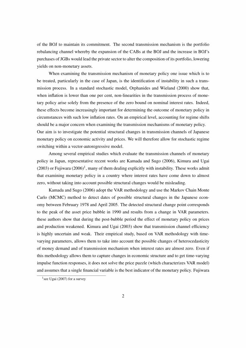
Since the beginning of the 1990s Japan has been experiencing a long economic slump
in addition to a deflation activated by the burst of the financial bubble. In order to try and
get out of this crisis, the bank of Japan (BOJ) began to cut rates reducing the uncollateralized
overnight call rate from 6 % in 1990 to 0.5 % in 1995 and then maintained this rate at such
level from September 1995 to September 1998, as shown by Figure1. Despite several short
Figure 1. CPI inflation and GDP growth rate
OUTPUT INFLATION
1986 1988 1990 1992 1994 1996 1998 2000 2002 2004 2006-15
-10
-5
0
5
10
15
recovery phases the economy began to deteriorate again in 1998. The BOJ then successively
decreased the call rate to a level very close to zero in 1999 and implemented the so-called Zero
Interest Rate Policy (henceforth ZIRP) between April 1999 and August 2000. The ZIRP was
defined as a commitment to maintain the uncollateralized overnight call rate at zero as long as
the economy is in deflation. This policy seemed to generate the expected results ; as shown by
Figure 1 the economy was recovering in mid-2000 and prices were at least stable. Therefore, the
BOJ decided to stop the ZIRP in August 2000. However, the economy weakened in late 2000 ;
5
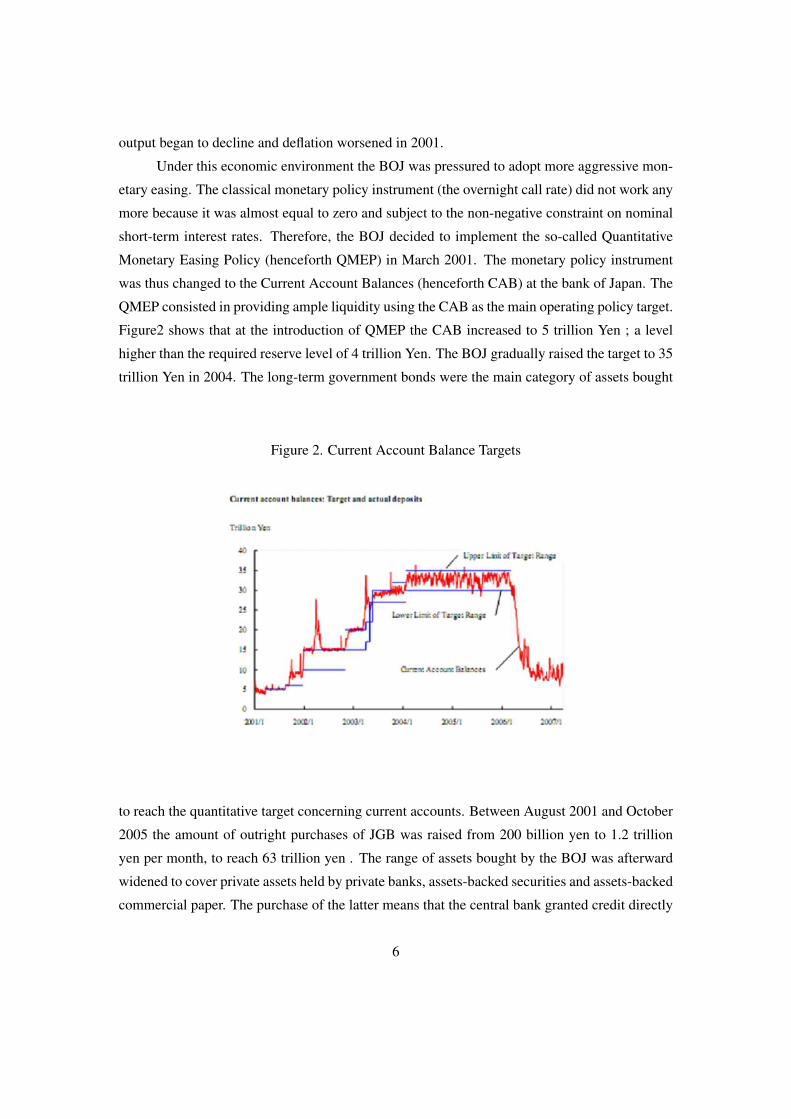
output began to decline and deflation worsened in 2001.
Under this economic environment the BOJ was pressured to adopt more aggressive mon-
etary easing. The classical monetary policy instrument (the overnight call rate) did not work any
more because it was almost equal to zero and subject to the non-negative constraint on nominal
short-term interest rates. Therefore, the BOJ decided to implement the so-called Quantitative
Monetary Easing Policy (henceforth QMEP) in March 2001. The monetary policy instrument
was thus changed to the Current Account Balances (henceforth CAB) at the bank of Japan. The
QMEP consisted in providing ample liquidity using the CAB as the main operating policy target.
Figure2 shows that at the introduction of QMEP the CAB increased to 5 trillion Yen ; a level
higher than the required reserve level of 4 trillion Yen. The BOJ gradually raised the target to 35
trillion Yen in 2004. The long-term government bonds were the main category of assets bought
Figure 2. Current Account Balance Targets
to reach the quantitative target concerning current accounts. Between August 2001 and October
2005 the amount of outright purchases of JGB was raised from 200 billion yen to 1.2 trillion
yen per month, to reach 63 trillion yen . The range of assets bought by the BOJ was afterward
widened to cover private assets held by private banks, assets-backed securities and assets-backed
commercial paper. The purchase of the latter means that the central bank granted credit directly
6
to small and medium-sized firms.
1.2 Transmission Mechanisms of QEPM
Several factors limited the number of monetary policy transmission channels in Japan.
First, because the nominal interest rates were almost zero the real interest rate could only be
affected by expected inflation. Consequently the conventional monetary policy using the tra-
ditional channel of the short-term interest rate is inoperative. Second, the Japanese banking
system collapse made the credit channel inefficient. Indeed, bank lending declined during the
period between 1999 and 2005 in spite of the ample liquidity provided to the banking system (Ito
and Mishkin (2004)). Third, another transmission channel through which monetary policy could
influence prices is the change of the value of domestic currency in the foreign exchange market.
This strategy was supported especially by Svensson (2003) and called the "foolproof way" to exit
the deflation spiral. Monetary authorities were skeptical about this strategy which was criticized
by Ito and Mishkin (2004) concerning its implementation. Indeed, after the adoption of floating
exchange rates as a rule of the international monetary system it became impossible to Japanese
authorities to follow Svenson’s suggestion. On the other hand, the implementation of exchange
rate peg could be a source of confusion between the nominal anchor, which is price level, and
exchange rate. However, Ito and Mishkin (2004) suggest that the Ministry of Finance and the
BOJ can intervene in the foreign exchange market without announcing an exchange rate target.
This intervention, being unsterilized, could help monetary authorities to gain in credibility send-
ing a signal that the main objective remains the price level. Ito and Yabu (2007) showed that the
amount of intervention during the period between 1999 and 2004 has became large but the effect
of such intervention weakened. The conjunction of these factors induces monetary authorities
and economists to look for other possible channels. By the implementation of QEMP the econ-
omy could be affected through other transmission mechanisms. We classify3 these transmission
channels in two groups: expectation effects and portfolio rebalancing effects.
1.2.1 Expectation effects
This transmission channel is strictly connected to the commitment to maintain a zero
interest rate until the rate of change of core CPI inflation becomes zero or positive year-on-year.
• Policy duration effect : although short interest rates are almost zero the QEMP allowed
3There are several possible way to classify transmission channels. See also Ugai (2007)
7
to cut these rates further . The overnight call rate reached an extremely low level (0,001
%) ; below the 0.02-0.03% that was realized under the ZIRP. Nevertheless, this tradition-
nel channel depends on the real interest rate, rather than the nominal one, which affects
the decisions of consumers and firms. Besides, it is the real long-term interest rate, and
not short-term, that is often considered as having a major incidence on the economy. The
relationship between short and long term real interest rates is explained by rational ex-
pectations. This expectation is possible only if the BOJ commits itself to maintaining a
permanent increase in the monetary base. This increase in the monetary base could raise
inflation expectations and afterwards could lead to a rise in spending (Krugman 2000) and
a fall in the long term real interest rate stimulating agregate demand. Moreover, commit-
ment would decrease the long term nominal interest rate when the private sector expects
that the nominal interest rate would be zero until the conditions of the commitment are
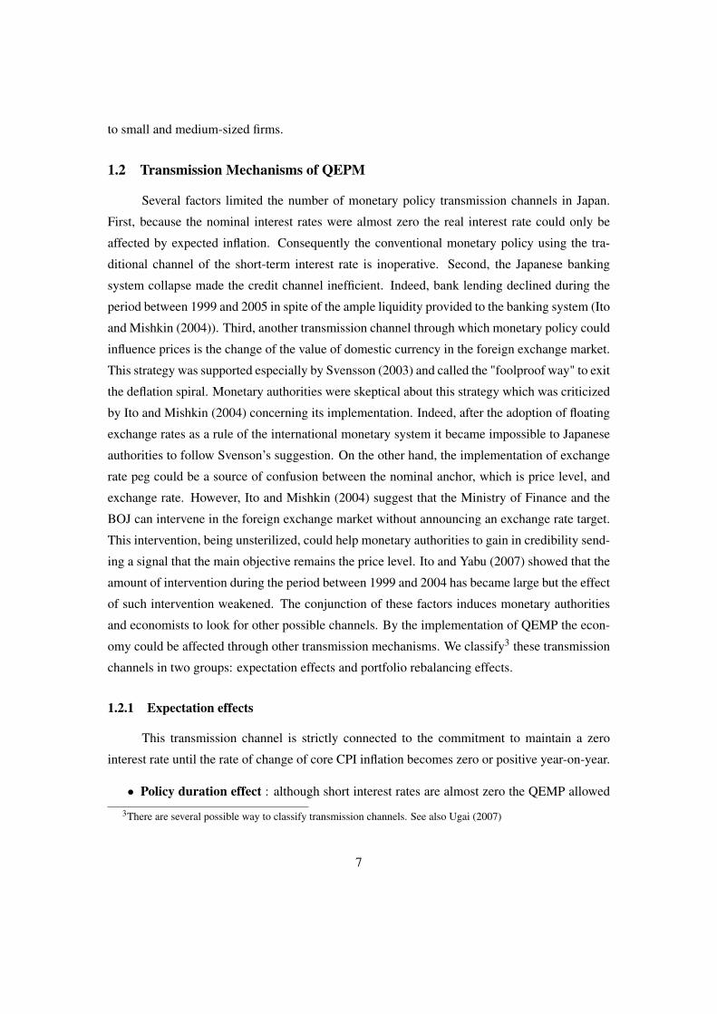
fullfilled. This so-called policy duration effect is reflected in the yield curve as shown by
Figure 3 The yield curves gradually flattened till the end of year 2005, reflecting the effect
of the credibility of the commitment of the BOJ on the anticipations of private agents.
• Signaling effect : signaling, in the Japanese monetary policy context, refers to the BOJ
providing ample information on the intended state of monetary conditions, both now and
into the future. All of the three pillars of QEMP may have a signaling effect. However,
the most important signal of the QEMP is the purchase of long-term JGBs. If private
agents suspects authorities renouncing on their commitment the objective of the inflation
becomes inefficient4. In this case the BOJ needed to send a more pronounced signal to the
private sector, making the commitment constraining. Indeed, when the BOJ increases its
purchases of long-term government bonds the credibility of maintaining its commitment
increases. In other words, the continuation of deflation would generate capital losses for
central bank. However, the private sector could also anticipate that the BOJ would incur
a capital loss, even if the commitment is maintained, when the long-term JGB interest
rate increases following an economic recovery and when the central bank tries to absorb
liquidity once the deflation process is stopped by selling JGB.
4Eggertsson and Woodford (2003) shows that the increase of monetary base does not influence the expected future
conduct of the monetary policy.
8
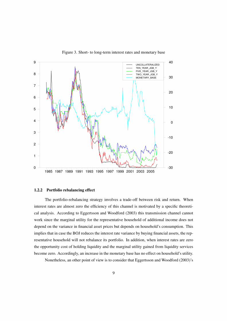
Figure 3. Short- to long-term interest rates and monetary base
1985 1987 1989 1991 1993 1995 1997 1999 2001 2003 20050
1
2
3
4
5
6
7
8
9
-30
-20
-10
0
10
20
30
40UNCOLLATERALIZED
TEN_YEAR_JGB_Y
FIVE_YEAR_JGB_Y
TWO_YEAR_JGB_Y
MONETARY_BASE
1.2.2 Portfolio rebalancing effect
The portfolio-rebalancing strategy involves a trade-off between risk and return. When
interest rates are almost zero the efficiency of this channel is motivated by a specific theoreti-
cal analysis. According to Eggertsson and Woodford (2003) this transmission channel cannot
work since the marginal utility for the representative household of additional income does not
depend on the variance in financial asset prices but depends on household’s consumption. This
implies that in case the BOJ reduces the interest rate variance by buying financial assets, the rep-
resentative household will not rebalance its portfolio. In addition, when interest rates are zero
the opportunity cost of holding liquidity and the marginal utility gained from liquidity services
become zero. Accordingly, an increase in the monetary base has no effect on household’s utility.
Nonetheless, an other point of view is to consider that Eggertsson and Woodford (2003)’s
9
assumption does not hold and thus marginal utility for the representative household depends on
the variance in financial asset prices with an imperfect substitutability of financial assets. There-
fore, following an increase of monetary base the marginal value of liquidity service reduces.
Because the representative household starts to adjust his portfolio by buying financial assets
with higher marginal values, these asset prices rise.
Besides, the resumption of inflation since November 2005 (Figure1) is a sign that the
QEMP may have been successful. The BOJ committed itself to maintaining this policy until
inflation (measured by the CPI excluding perishables) is stably positive. It predicted in March
2006 that the inflation would remain positive and judged that the objective was reached and that
it was time to exit the QEMP. Consequently, the BOJ returned to the traditional instrument, the
overnight interest rate, as the operating target. Nevertheless, the efficacy of QEMP has not been
definitively established empirically. We suggest below to evaluate empirically the effects of such
a policy on the real economy through the channels just cited.
2 Methodology
Several criticisms adressed to the VAR approach concerning the identification of the mon-
etary policy concentrate on the use of a restricted quantity of information. To optimize the degree
of freedom, it is rare to use more than eight variables in a classical VAR model.
Bernanke et al. (2005) showed that the lack information from which the VAR approach
traditionally suffers leads at least to two problems. First, taking into account only a small num-
ber of variables in the analysis biases the measures of the shocks of monetary policy. The best
illustrations of this problem are price, interest rate, liquidity and exchange rate puzzles. Second,
the impulse response functions are observed only for variables included in the model. The anal-
ysis cannot thus be done on global economic concepts like economic activity or productivity,
which cannot be represented by a single variable. To remedy these problems, the authors pro-
posed a combination between the factor analysis and the VAR analysis. This approach allows us
to summarize a large amount of information in a limited number of factors which will be used in
the VAR model. This method, FAVAR, has the advantage of introducing the maximum quantity
of information which is taken into account by central banks and private agents, while respecting
the constraint of degrees of freedom of the model. Moreover, it avoids imprecision and possible
biases in the estimates that arise from the fact that any one observable may be a poor measure of
the relevant underlying concept.
However, in Bernanke et al. (2005)’s paper the factors do not have an immediate economic
10
interpretation. Following Belviso and Milani (2006) we provide a structural interpretation to
these factors. We seek to identify each factor as a basic force that governs the economy as ‘real
activity’, ‘price pressure’, ‘interest rates’, ‘credit sector’, and so on. We follow this literature
and attempt to go a step further, seeking to take into account the possible existence of structural
change in the monetary transmission mechanism. We therefore propose a Markov switching
vector autoregression augmented with economically interpretable factors: we label this novel
approach Markov Switching S-Structural Factor-Augmented VAR (MS-SFAVAR).
2.1 MS-FAVAR
Let Xt and Yt be two vectors of economic variables, with dimensions (NX1) and (MX1).
and where t = 1,2, ...T is a time index. Xt denotes the large dataset of economic variables and
Yt denotes the monetary policy instrument controlled by the central bank. We assume that Xt are
related to a vector Ft with (KX1) unobservable factors, as follows :
Xt = Λf Ft + et (2.1)
where et are errors with mean zero assumed to be either weakly correlated or uncorrelated ;
these can be interpreted as the idiosyncratic components. The (NXK) vector Λ represents the
factor loadings.The main advantage of this static representation of the dynamic factor model,
described by equation 2.1, is that factors can be estimated by the principal component method.
We can think of unobservable factors in terms of concepts such as “economic activity” or “price
pressure”. But here, following Belviso and Milani (2006) we divide Xt into various categories
X1t , X2
t , ... X It which represent various economic concepts where X i
t is a (NiX1) vector and
∑i Ni = N. Each category of X it is thus assumed to be represented by only one element of F i
t
which is a (KiX1) vector (∑i Ki = K). That means that each of the variables in the vector X it
is influenced by the state of the economy only through the corresponding factors. Therefore,
compared to the FAVAR model, the factors have more meaningful structural interpretations.
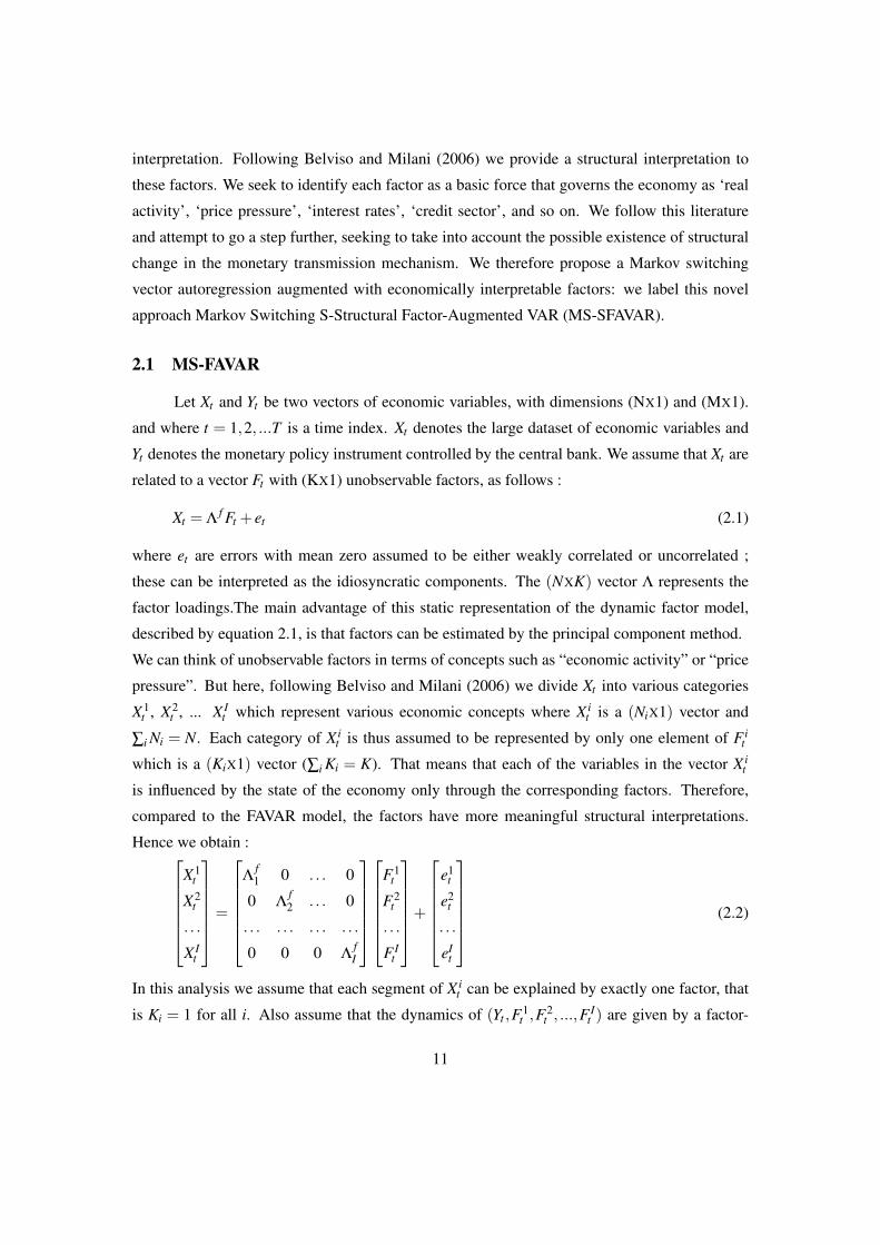
Hence we obtain :X1
t
X2t
. . .
X It
=
Λ
f1 0 . . . 0
0 Λf2 . . . 0
. . . . . . . . . . . .
0 0 0 ΛfI
F1
t
F2t
. . .
F It
+
e1
t
e2t
. . .
eIt
(2.2)
In this analysis we assume that each segment of X it can be explained by exactly one factor, that
is Ki = 1 for all i. Also assume that the dynamics of (Yt ,F1t ,F2
t , ...,F It ) are given by a factor-
11
augmented autoregression (FAVAR):
F1t
F2t
. . .
F It
Yt
= Φ(L)
F1t−1
F2t−1
. . .
F It−1
Yt−1
+νt (2.3)
Consider the (M + I)X1 dimensional vector Zt :
Zt =t[
F1t F2
t . . . F It Yt
](2.4)
A Markov-Switching structural factor-augmented VAR is described by equation 2.5. In its most
popular version (Krolzig (1997)), which we will use here, the regime-switching model assumes
that the process st is a first-order Markov process. Hamilton (1989)’s original specification
assumed that a change in regime corresponds to an immediate one-time jump in the process
mean. We rather consider the possibility that the mean would smoothly approach a new level
after the transition from one regime to another . We do it in an extension of Hamilton’s approach
to a regime-switching VAR system (Krolzig (1997)).
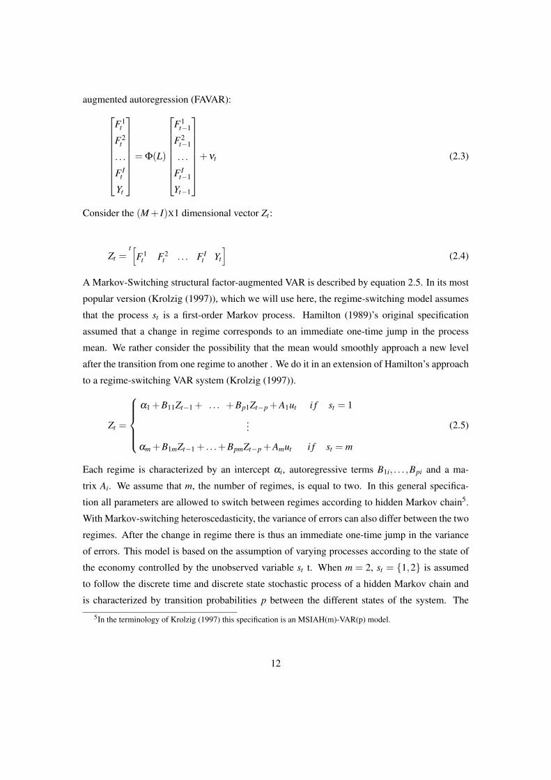
Zt =
α1 +B11Zt−1 + . . . +Bp1Zt−p +A1ut i f st = 1
...
αm +B1mZt−1 + . . .+BpmZt−p +Amut i f st = m
(2.5)
Each regime is characterized by an intercept αi, autoregressive terms B1i, . . . ,Bpi and a ma-
trix Ai. We assume that m, the number of regimes, is equal to two. In this general specifica-
tion all parameters are allowed to switch between regimes according to hidden Markov chain5.
With Markov-switching heteroscedasticity, the variance of errors can also differ between the two
regimes. After the change in regime there is thus an immediate one-time jump in the variance
of errors. This model is based on the assumption of varying processes according to the state of
the economy controlled by the unobserved variable st t. When m = 2, st = {1,2} is assumed
to follow the discrete time and discrete state stochastic process of a hidden Markov chain and
is characterized by transition probabilities p between the different states of the system. The
5In the terminology of Krolzig (1997) this specification is an MSIAH(m)-VAR(p) model.
12
probability may be written
pi, j = Pr(st+1 = j|st = i),2
∑j=1
pi j = 1∀i, j ∈ (1,2). (2.6)
This stochastic process is defined by the transition matrix P as follows:
p =
(p11 p12
p21 p22
)(2.7)
For a given parametric specification of the model, probabilities are assigned to the unobserved
economic regimes conditional on the available information set which constitutes an optimal
inference on the latent state of the economy. We thus obtain the probability of staying in a
given regime when starting from that regime, as well as the probability of shifting to another
regime. The classification of regimes and the dating of Japanese economy periods imply that
every observation in the sample is assigned to one of the two regimes. The rule followed to
assign an observation at time t to a specific regime depends on the highest smoothed probability.
The smoothed probability of being in a given regime is computed by using all the observations
in the sample. We assign an observation to a specific regime when the smoothed probability of
being in that regime is higher than one half.
2.2 Estimation
Our MS-SFAVAR approach retains the advantages of a FAVAR model over a simple VAR.
Moreover, it allows us to take into account the instability of the monetary transmission mech-
anism. Factors estimated from the subset databases are the unobserved variables that, with the
policy instrument, enter in the MS-VAR (equation 2.5). To estimate the factors, the variables
must be transformed to induce stationarity. It is important to note that the variables used in VAR
analysis do not need to be stationary. In the tradition of Sims et al. (1990), the specification of a
VAR system that we use considers variables in levels. In the case of such VARs with polynomial
functions of time and one or more unit roots, Sims et al. (1990) showed that, independently of
the order of integration of the variables, one can get a consistent estimation of coefficients. An
alternative route would consist in focusing on target variables such as the output gap rather than
the level of output, and inflation rather than the price level. However, both would raise problems.
In the case of Japan, the output gap is a loosely defined concept since there is much uncertainty
as to the level of potential output (Kamada and Masuda (2001); and Bayoumi (2001)). Similarly,
focusing on the rate of inflation would not seem adequate when examining a period of overall
13
price stability. Movements in the price level then seem to be the relevant variable of interest.
Consequently, we estimate model in levels using cumulative factors.
In this paper we consider a two-step approach to estimating 2.2-2.5. The first step consists
of the estimation of the factors and factor loadings. The second step is the estimation of the MS-
VAR using the factors.
2.2.1 Factor estimation
The main approach used for the estimation of factors consist of principal component anal-
ysis. However, As discussed by Eliatsz (2002) and Belviso and Milani (2006), the factors esti-
mated by principal component have unknown dynamic properties because principal components
do not exploit the dynamics of the factors or the dynamic of the idiosyncratic component. There
are two principal approaches that exploit these features to extract the static factors through prin-
cipal components. The first is the two-step approach situated in the frequency domain proposed
by Forni and Reichlin (2005). This approach exploits the cross-sectional heteroscedasticity of
the idiosyncratic component and the dynamic properties of the data when extracting the com-
mon factors. A similar strategy has been proposed by Stock and Watson (2002). The second ap-
proach, a two-step strategy in the parametric time domain introduced by Giannone et al. (2005)
and developed by Doz et al. (2006), uses principal components and the Kalman smoother to
exploit both factor dynamics and idiosyncratic heteroscedasticity.
For the MS-SFAVAR approach employed in this paper, static factors are estimated by
using the Doz et al. (2006) method. As explained above the two step estimator of approxi-
mate factor models outperforms the principal component method in a finite sample, but only
if the sample size is large enough 6. However Bernanke et al. (2005) and Belviso and Milani
(2006) showed that the results under the two-step principal component approach are quite close
to Bayesian joint estimation. Moreover, the two-step approach implies uncertainty surrounding
the factor estimation. To obtain accurate confidence intervals on the impulse response functions,
following Bernanke et al. (2005) we carry out a bootstrap procedure that accounts for the uncer-
tainty in the factors. Bai and Ng (2002) provide some criteria to choose the number of factors,
but no criterion has been developed to determine the optimal number of factors in a VAR frame-
work. We assume only a single factor from each group in our MS-SFAVAR model in this paper.
We divide Xt so that each sub-group is represented by only one of the following structural factors
:6According to Doz et al. (2006) 7O variables is a minimum.
14
• Real Activity factor : represents the general economic concept of “economic activity”
instead of the single indicator of industrial production. It captures variances in the individ-
ual series such as industrial production, capacity utilization, employment / unemployment
rates, new orders, housing starts,...
• Inflation factor : consists in the concept of ’inflation’. It is driven by the evolution of
consumer prices, corporate goods and services prices.
• Interest rate factor : represents some interest rates of various maturity.
2.2.2 MS-FAVAR estimation
In the second step the model is estimated through the EM7 (Expectation–Maximization)
algorithm. Estimated factors are introduced in 2.5 instead of variables in a classical MS-VAR
model.
In a Markov-switching VAR, with regime-dependence in the mean, variance and autoregressive
parameters, a large number of parameters can potentially switch between regimes. It is there-
fore often difficult to interpret the results of the estimation of such systems. Such a problem
of interpretation is similar to the interpretation of parameters in simple VAR systems. Since
the seminal work of Sims (1980), econometricians have traditionally imposed identifying re-
strictions on the parameters estimates. They then derive a structural form of the model based
on economic intuition. This approach uses impulse response analysis in order to trace out how
fundamental disturbances affect variables in the model. Recently Ehrmann et al. (2003) sug-
gested imposing similar identifying restrictions on Markov-switching models. They propose
using regime-dependent impulse response functions in order to trace out how fundamental dis-
turbances affect the variables in the model, dependent on the regime. As a result, there is a set
of impulse response functions for each regime. Such response functions are conditional on a
given regime prevailing at the time of the shock and throughout the duration of the response8.
They facilitate the interpretation of switching parameters by providing a convenient way to sum-
marise the information contained in the autoregressive parameters, variances and covariances of
each regime. This approach combines Markov-switching and identification in a two-stage pro-
cedure of estimation and identification. First, a Markov-switching unrestricted VAR model is
7The estimation method, identification and impulse response are detailed in Ehrmann et al. (2003)8As shown by Ehrmann et al. (2003) regimes predicted by the transmission matrix must be highly persistent in
order to have useful regime dependent impulse functions.
15
estimated, allowing means, intercepts, autoregressive parameters, variances and covariances to
switch. Estimation of the Markov-switching model uses expected maximum likelihood (Hamil-
ton (1989) and Hamilton (1994)) because the recursive nature of the likelihood, stemming from
the hidden Markov Chain, precludes likelihood maximization with standard techniques. Second,
in order to identify the system, one can impose restrictions on the parameter estimates to derive
a separate structural form for each regime, from which it is possible to compute the regime-
dependent impulse response functions. Identification uses the Cholesky decomposition of the
variance-covariance matrix. The confidence intervals around the impulse responses are com-
puted by bootstrapping techniques. The latter involve the creation of artificial histories for the
variables and submitting such histories to the same estimation procedure as the data Ehrmann
et al. (2003).
3 Empirical Analysis
In the following, we report the results from the estimation of a MS-SFAVAR model on a
data set including 3 sub-groups of factors, representing 3 economic concepts, and a monetary
policy instrument. Our sample Xt contains 143 variables and spans from 1985 : 3 to 2006 : 10 at
a monthly frequency. The standard method to evaluate monetary policy through a VAR model is
to consider the uncollateralized overnight call interest rate as monetary policy instrument. In the
special case of Japan, where interest rates are almost equal to zero and where the BOJ cannot
control them this method cannot be applied, because interest rates contain no more information
concerning the behavior of monetary policy. Theoretical work investigated alternative variables,
so-called intermediate variables, which are not directly controlled by the central bank. These
variables can be the long-term interest rate, the exchange rate, the interest rate spread and the
monetary policy proxy (Kamada and Sugo (2006))9. Nevertheless, intermediate variables can be
inconvenient as far as they can react to their own shocks, thereby complicating the identification
of the shocks of the monetary policy. In this paper, we use the monetary base10 as the monetary
policy instrument to measure the effect of the quantitative easing policy in Japan. The monetary
base thus represents the only observed factor included in Yt .
9The monetary policy proxy was constructed by combining two intermediate variables namely lending rates and
the lending attitude of financial institutions.10Kimura and Ugai (2003) and Fujiwara (2006)
16
3.1 Estimated Structural Factors
The first obvious check of the fit of our factors model is to see how well each factor
represents each sub-group of data series. In particular we examine the assumption according
to which every sub-group is represented by only one factor. To this end, for every variable of
each sub-group we estimate the R2 from regressing each series onto the first and the second
corresponding factors. Results11 show that there is a large difference between the first factor and
the second one in each group in terms of variance explained. Therefore, in each sub-group the
first factor corresponds to the biggest variance explained. The small gain in the percentage of
the variance explained, when adding a second factor, confirms the robustness of our assumption
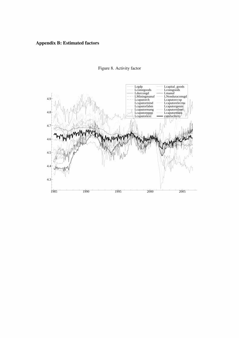
considering only one factor for each sub-group. Figure 8, 9 and 10 reported in the Appendix B
demonstrate that cumulative factors seem to sufficiently present the corresponding variables in
level.
3.2 Traditional MS-VAR
We first evaluate Japanese monetary policy using the MS-VAR model following Fujiwara
(2006) with four variables such as output y, the price level p,the money stock m and bond yields
l with a longer sample. The main difficulty concerns the determination of the number of regimes
which characterize better the behavior of the studied time series. In a second step the best
specification among various MS-VAR model should be determined.
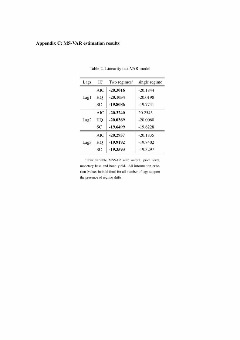
The test for linearity by taking the linear model as the null hypothesis (there is a single
regime) and the regime-switching model as the alternative. The usual tests, namely LR tests,
LM and Walds tests, cannot be conducted since the nuisance parameter is identified only under
the alternative. Several works studied the problem of statistical inference when the nuisance
parameters are non-identified under the null hypothesis. Hansen (1992) and Garcia (1998) pro-
posed a non-standard likelihood ratio test (NSLR). This test is calculated as a correction on the
p-value of a standard likelihood ratio test. This method does not give exact critical values but
only a lower bound for the limiting distribution of a standard LR statistic. Since the null pa-
rameter space contains only two subsets Cho and White (2007) showed that the NSLR test is
not valid if the boundary conditions are ignored. Moreover, Cho and White (2007)’s test (QLR)
is applicable on specific models which do not include the MSVAR. In this paper we therefore
perform other tests like Log-likelihood or information criterion. The null hypothesis is clearly
11The results are available upon request.
17
rejected as shown in Table 2 in the Appendix C. The two regime model is therefore maintained.
In next step we identify the best specification among various MS-VAR models. In this
case the LR test can performed without causing problem. The alternative hypothesis MSIAH-
VAR specification is tested against the other possible specifications namely MSI, MSIA and
MSIH models for different lags.
The likelihood ratio test (Appendix C, Table3) suggests that an MSIAH-VAR model fits
better the data than others MSI-VAR specifications for two and three lags. Consequently, the
study applies the Markov switching MSIAH-VAR model in which intercepts, parameters au-
toregressions and variance covariance matrices are allowed to switch between regimes. The lag
length is chosen to be two in order to have serially uncorrelated residuals. This lag length is
supported by AIC and HQ criterion (Appendix C, Table4). Next, according to Table 5 in the
Appendix C that shows the transition matrix, the two regimes are highly persistent. Regime
dependent impulse responses will then be an interesting tool to analyze the monetary policy of
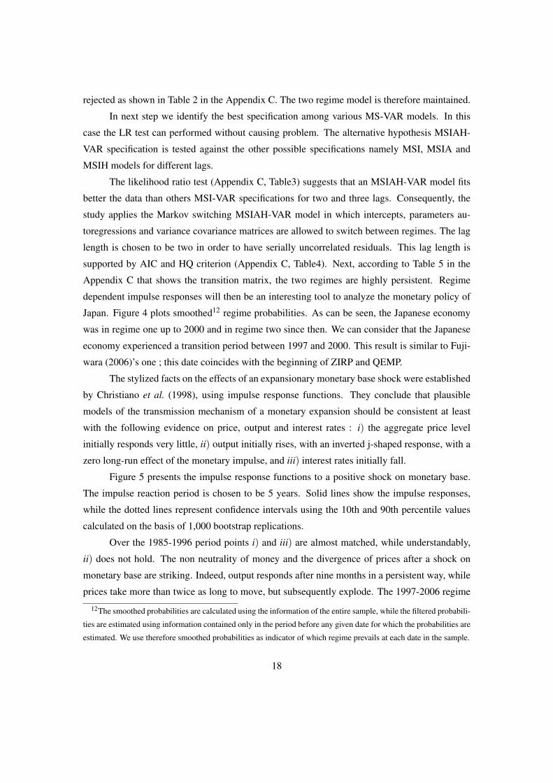
Japan. Figure 4 plots smoothed12 regime probabilities. As can be seen, the Japanese economy
was in regime one up to 2000 and in regime two since then. We can consider that the Japanese
economy experienced a transition period between 1997 and 2000. This result is similar to Fuji-
wara (2006)’s one ; this date coincides with the beginning of ZIRP and QEMP.
The stylized facts on the effects of an expansionary monetary base shock were established
by Christiano et al. (1998), using impulse response functions. They conclude that plausible
models of the transmission mechanism of a monetary expansion should be consistent at least
with the following evidence on price, output and interest rates : i) the aggregate price level
initially responds very little, ii) output initially rises, with an inverted j-shaped response, with a
zero long-run effect of the monetary impulse, and iii) interest rates initially fall.
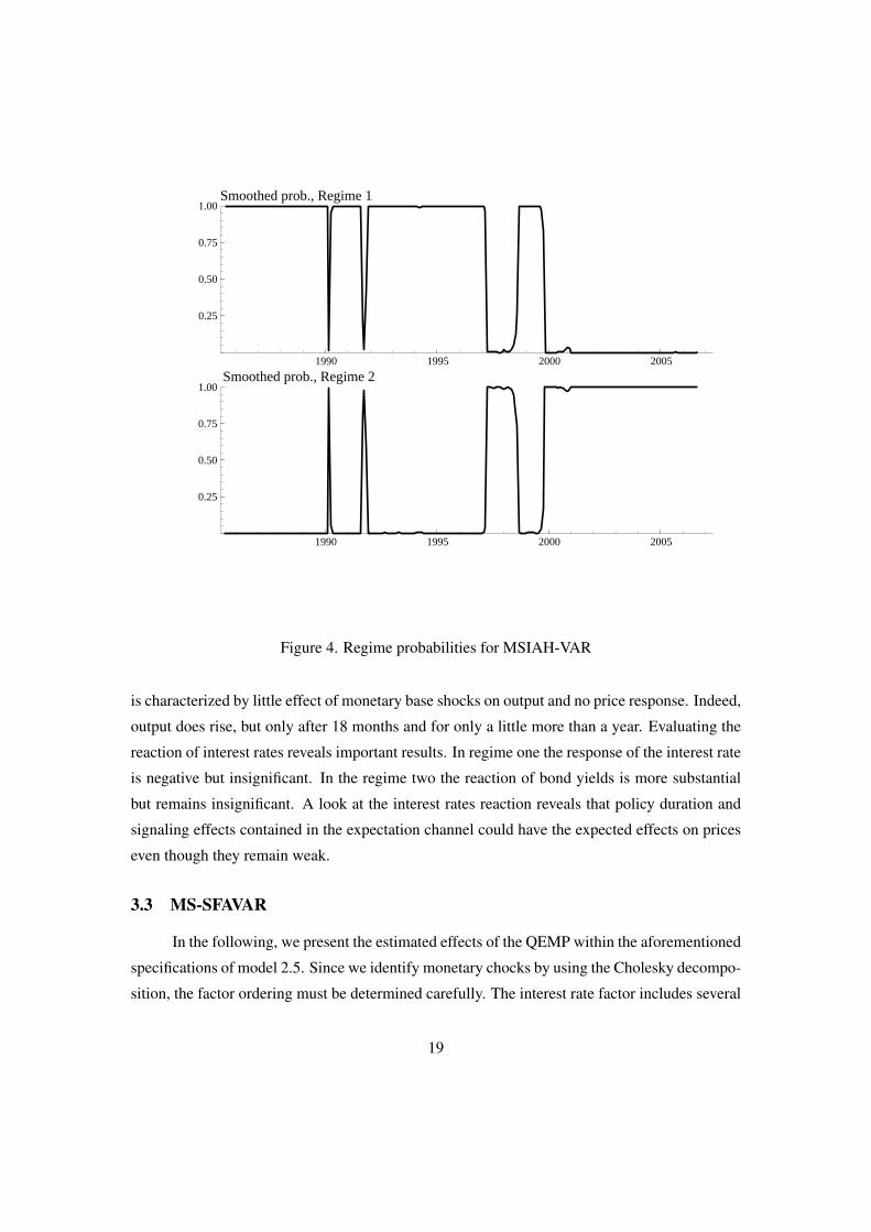
Figure 5 presents the impulse response functions to a positive shock on monetary base.
The impulse reaction period is chosen to be 5 years. Solid lines show the impulse responses,
while the dotted lines represent confidence intervals using the 10th and 90th percentile values
calculated on the basis of 1,000 bootstrap replications.
Over the 1985-1996 period points i) and iii) are almost matched, while understandably,
ii) does not hold. The non neutrality of money and the divergence of prices after a shock on
monetary base are striking. Indeed, output responds after nine months in a persistent way, while
prices take more than twice as long to move, but subsequently explode. The 1997-2006 regime
12The smoothed probabilities are calculated using the information of the entire sample, while the filtered probabili-
ties are estimated using information contained only in the period before any given date for which the probabilities are
estimated. We use therefore smoothed probabilities as indicator of which regime prevails at each date in the sample.
18
1990 1995 2000 2005
0.25
0.50
0.75
1.00Smoothed prob., Regime 1
1990 1995 2000 2005
0.25
0.50
0.75
1.00Smoothed prob., Regime 2
Figure 4. Regime probabilities for MSIAH-VAR
is characterized by little effect of monetary base shocks on output and no price response. Indeed,
output does rise, but only after 18 months and for only a little more than a year. Evaluating the
reaction of interest rates reveals important results. In regime one the response of the interest rate
is negative but insignificant. In the regime two the reaction of bond yields is more substantial
but remains insignificant. A look at the interest rates reaction reveals that policy duration and
signaling effects contained in the expectation channel could have the expected effects on prices
even though they remain weak.
3.3 MS-SFAVAR
In the following, we present the estimated effects of the QEMP within the aforementioned
specifications of model 2.5. Since we identify monetary chocks by using the Cholesky decompo-
sition, the factor ordering must be determined carefully. The interest rate factor includes several
19
0 1 2 3 4 5
−0.5
0.0
0.5 Y
0 1 2 3 4 5
0.00
0.25Y
0 1 2 3 4 5
0.0
0.1
0.2
0.3P
0 1 2 3 4 5
0.0
0.1 P
0 1 2 3 4 5
0.5
1.0
1.5MB
0 1 2 3 4 5
0
1MB
0 1 2 3 4 5
−0.05
0.00
0.05 Bond yields
0 1 2 3 4 5
−0.05
0.00
0.05Bond yields
Figure 5. Impulse responses to a monetary shock for MS-VAR
long-term rates that contain expectations on economy. Because the monetary authorities can re-
act only to the current state of the economy, the interest rate factor is ordered after the monetary
base. We consider therefore the following ordering of factors : real activity factor, prices factor,
monetary base and interest rate factor. Information criteria (Appendix D, Table6) suggest that
the model is non-linear.
From table 7 and table 8 in the Appendix D, a MSIAH-FAVAR specification is suggested
by the LR test and the lag length supported by two information criteria is two. As can be seen
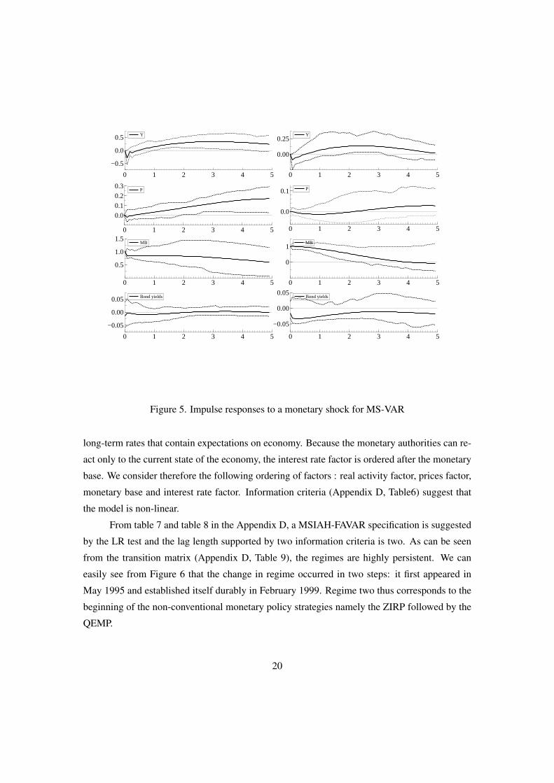
from the transition matrix (Appendix D, Table 9), the regimes are highly persistent. We can
easily see from Figure 6 that the change in regime occurred in two steps: it first appeared in
May 1995 and established itself durably in February 1999. Regime two thus corresponds to the
beginning of the non-conventional monetary policy strategies namely the ZIRP followed by the
QEMP.
20
1985 1990 1995 2000 2005
0.25
0.50
0.75
1.00
Smoothed prob., regime 1
1985 1990 1995 2000 2005
0.25
0.50
0.75
1.00
Smoothed prob., regime 2
Figure 6. Regime probabilities for MS-FAVAR
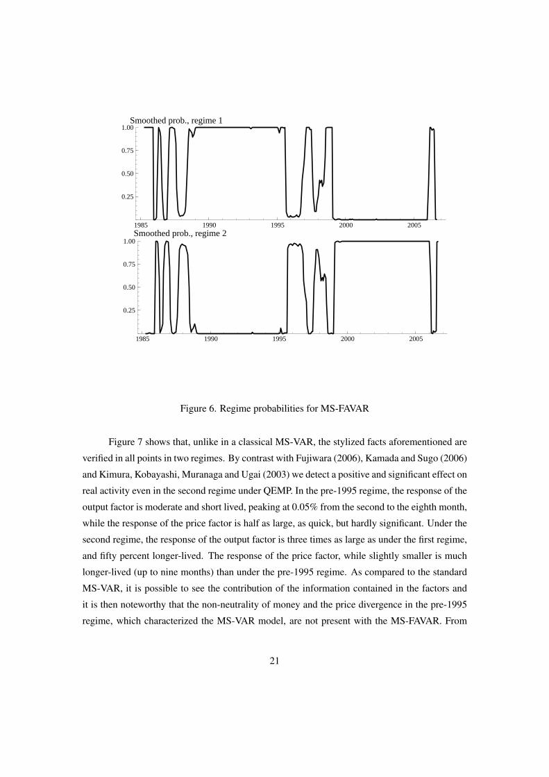
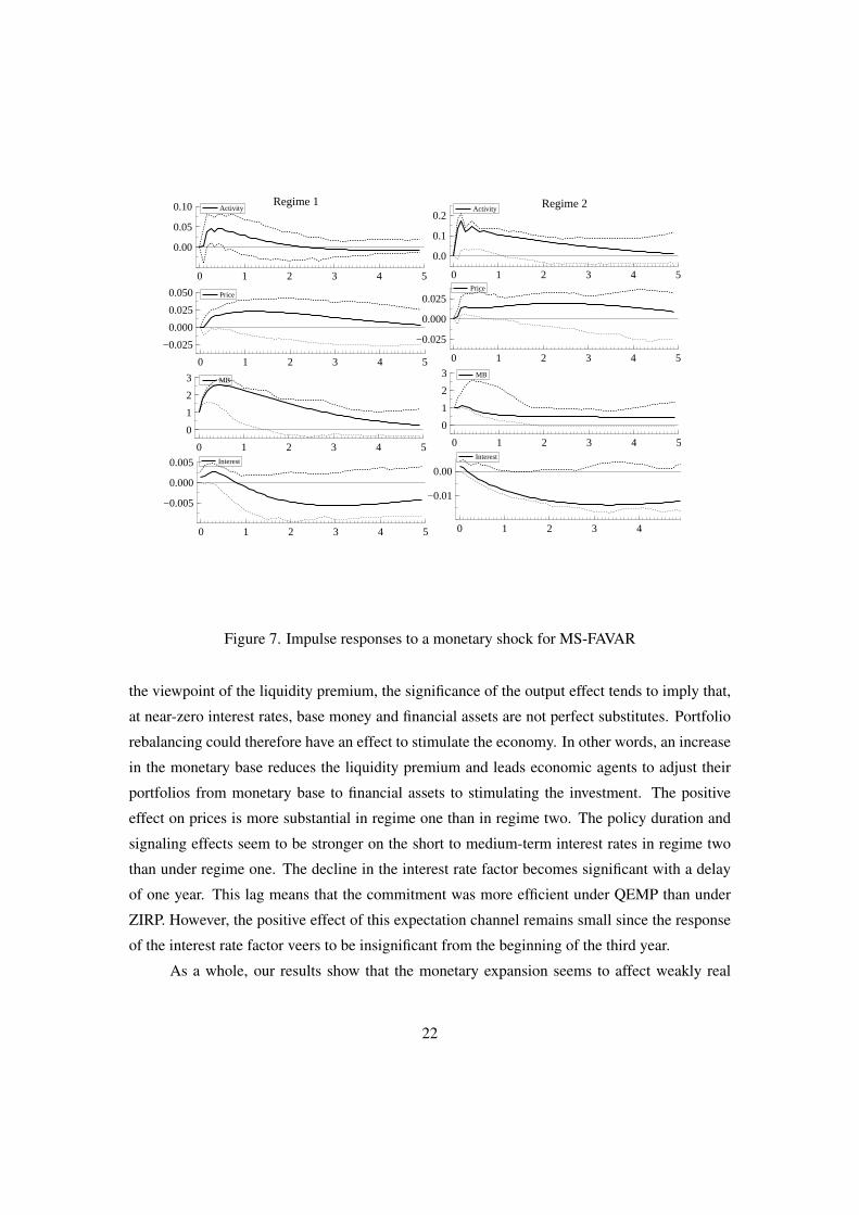
Figure 7 shows that, unlike in a classical MS-VAR, the stylized facts aforementioned are
verified in all points in two regimes. By contrast with Fujiwara (2006), Kamada and Sugo (2006)
and Kimura, Kobayashi, Muranaga and Ugai (2003) we detect a positive and significant effect on
real activity even in the second regime under QEMP. In the pre-1995 regime, the response of the
output factor is moderate and short lived, peaking at 0.05% from the second to the eighth month,
while the response of the price factor is half as large, as quick, but hardly significant. Under the
second regime, the response of the output factor is three times as large as under the first regime,
and fifty percent longer-lived. The response of the price factor, while slightly smaller is much
longer-lived (up to nine months) than under the pre-1995 regime. As compared to the standard
MS-VAR, it is possible to see the contribution of the information contained in the factors and
it is then noteworthy that the non-neutrality of money and the price divergence in the pre-1995
regime, which characterized the MS-VAR model, are not present with the MS-FAVAR. From
21
0 1 2 3 4 5
0.0
0.1
0.2Regime 2 Activity
0 1 2 3 4 5
0.00
0.05
0.10 Regime 1Activity
0 1 2 3 4 5
−0.025
0.000
0.025Price
0 1 2 3 4 5
−0.025
0.000
0.025
0.050 Price
0 1 2 3 4 5
0
1
2
3 MB
0 1 2 3 4 5
0
1
2
3 MB
0 1 2 3 4 5
−0.01
0.00
Interest
0 1 2 3 4 5
−0.005
0.000
0.005 Interest
Figure 7. Impulse responses to a monetary shock for MS-FAVAR
the viewpoint of the liquidity premium, the significance of the output effect tends to imply that,
at near-zero interest rates, base money and financial assets are not perfect substitutes. Portfolio
rebalancing could therefore have an effect to stimulate the economy. In other words, an increase
in the monetary base reduces the liquidity premium and leads economic agents to adjust their
portfolios from monetary base to financial assets to stimulating the investment. The positive
effect on prices is more substantial in regime one than in regime two. The policy duration and
signaling effects seem to be stronger on the short to medium-term interest rates in regime two
than under regime one. The decline in the interest rate factor becomes significant with a delay
of one year. This lag means that the commitment was more efficient under QEMP than under
ZIRP. However, the positive effect of this expectation channel remains small since the response
of the interest rate factor veers to be insignificant from the beginning of the third year.
As a whole, our results show that the monetary expansion seems to affect weakly real
22
activity and prices. The effectiveness of quantitative easing remains limited, considering the
amount of liquidity injected in the economy and the effort made by the BOJ to gain in credibility
and to guide private sector expectation and behavior.
4 conclusion
During the Great Stagnation in Japan, academic economists almost unanimously recom-
mended that, under a liquidity trap, the only way for monetary authorities to try and revive
the economy was to force-feed banks with base money. In this paper we propose a FAVAR
approach combined with a Markov Switching method in order to analyze the effectiveness of
Japanese monetary policy. We implemented a two-step approach. In a first step, structural fac-
tors are estimated from subset databases representing different economic concepts. In a second
step, a Markov-switching model was estimated by EM algorithm method.
Three main conclusions can be drawn from this work. First, this paper is the first to show
that when the Bank of Japan did start to follow such advice, through its quantitative easing
policy, such a strategy did help revive output growth and price inflation. Such results contrast
with almost all available empirical evidence on the effects of such policy. Such a contrast does
not stem from our use of regime-switching analysis, but rather from our use of factor analysis
in order to account for the myriad of variables which may have been interacting and propelled
by this new monetary policy of the BOJ. Second, by contrast with the MS-VAR approach, our
MS-FAVAR allowed us to detect changes in monetary policy mechanism in a credible way ;
structural change occurred in February 1999 after a period of transition starting in May 1995.
Third, our results show that the non-neutrality of money and the price divergence in the pre-1995
regime, which characterized the MS-VAR model, are not present with the MS-FAVAR.
Results presented here confirm thus the idea that exploiting a larger and more realistic informa-
tion set reveals to be better to model the monetary policy behavior.
In future work, we plan to use this approach in order to investigate in detail the trans-
mission mechanism of Japanese monetary policy. The Interest rate factor seems to be operative
and responsible for the monetary policy influence. However, this factor can be affected by both
the expectation and the portfolio rebalancing channels suggested by the QEMP. It will be thus
interesting to determine the size of the effect of every transmission channel.
23
References
Bayoumi, Tamim. 2001. The morning after: explaining the slowdown in Japanese growth in
the 1990s. Journal of International Economics, 53(2), 241–259. http://ideas.repec.
org/a/eee/inecon/v53y2001i2p241-259.html.
Belviso, Francesco, and Milani, Fabio. 2006. Structural Factor-Augmented VARs (SFAVARs)
and the Effects of Monetary Policy. Topics in Macroeconomics, 6(3), 1443–1443. http:
//ideas.repec.org/a/bep/mactop/v6y2006i3p1443-1443.html.
Bernanke, Ben, Boivin, Jean, and Eliasz, Piotr S. 2005. "Measuring the Effects of Monetary Pol-
icy: A Factor-augmented Vector Autoregressive (FAVAR) Approach". The Quarterly Jour-
nal of Economics, 120(1), 387–422. http://ideas.repec.org/a/tpr/qjecon/
v120y2005i1p387-422.html.
Bernanke, Ben S. 2000. Comment on America’s Historical Experience with Low Inflation.
Journal of Money, Credit and Banking, 32(4), 994–97. http://ideas.repec.org/a/
mcb/jmoncb/v32y2000i4p994-97.html.
Cho, Jin Seo, and White, Halbert. 2007. Testing for Regime Switching. Econo-
metrica, 75(6), 1671–1720. http://ideas.repec.org/a/ecm/emetrp/
v75y2007i6p1671-1720.html.
Christiano, Lawrence J., Eichenbaum, Martin, and Evans, Charles L. 1998. Monetary Policy
Shocks: What Have We Learned and to What End? Feb. http://ideas.repec.org/
p/nbr/nberwo/6400.html.
Doz, Catherine, Giannone, Domenico, and Reichlin, Lucrezia. 2006. A Two-step estimator
for large approximate dynamic factor models based on Kalman filtering. http://ideas.
repec.org/p/ema/worpap/2006-23.html.
Eggertsson, Gauti B., and Woodford, Michael. 2003. The Zero Bound on Interest Rates and
Optimal Monetary Policy. Brookings Papers on Economic Activity, 34(2003-1), 139–235.
http://ideas.repec.org/a/bin/bpeajo/v34y2003i2003-1p139-235.
html.
Ehrmann, Michael, Ellison, Martin, and Valla, Natacha. 2003. Regime-dependent im-
pulse response functions in a Markov-switching vector autoregression model. Eco-
nomics Letters, 78(3), 295–299. http://ideas.repec.org/a/eee/ecolet/
v78y2003i3p295-299.html.
Forni, M., M. Hallin M. Lippi, and Reichlin, L. 2005. The generalized dynamic factor model:
one-sided estimation and forecasting. Journal of the American Statistical Association, 100.
Fujiwara, Ippei. 2006. Evaluating monetary policy when nominal interest rates are almost zero.
Journal of the Japanese and International Economies, 20(3), 434–453. http://ideas.
repec.org/a/eee/jjieco/v20y2006i3p434-453.html.
Giannone, Domenico, Reichlin, Lucrezia, and Small, David. 2005. Nowcasting GDP and
Inflation: The Real Time Informational Content of Macroeconomic Data Releases. Aug.
http://ideas.repec.org/p/cpr/ceprdp/5178.html.
Hamilton, James D. 1989. A New Approach to the Economic Analysis of Nonstationary Time
Series and the Business Cycle. Econometrica, 57(2), 357–84. http://ideas.repec.
org/a/ecm/emetrp/v57y1989i2p357-84.html.
Hamilton, James D. 1994. Rational Expectations and the Economic Consequences of Changes
in Regime. Nov. http://ideas.repec.org/p/cdl/ucsdec/94-24.html.
Ito, Takatoshi, and Mishkin, Frederic S. 2004. Two Decades of Japanese Monetary Policy and
the Deflation Problem. Nov. http://ideas.repec.org/p/nbr/nberwo/10878.
html.
Ito, Takatoshi, and Yabu, Tomoyoshi. 2007. What prompts Japan to intervene in the
Forex market? A new approach to a reaction function. Journal of International
Money and Finance, 26(2), 193–212. http://ideas.repec.org/a/eee/jimfin/
v26y2007i2p193-212.html.
Kamada, K., and Sugo, T. 2006. Evaluating the Japanese Monetary Policy under the Non-
Negativity Constraint on Nominal Short-Term Interests Rates. Sep.
Kamada, Koichiro, and Masuda, Kazuto. 2001. Effects of Measurement Error on the Output
Gap in Japan. Monetary and Economic Studies, 19(2), 109–54. http://ideas.repec.
org/a/ime/imemes/v19y2001i2p109-54.html.
Kimura, T., H. Kobayashi J. Muranaga, and Ugai, H. 2003. The Effect of the Increase in the
Monetary Base on Japan’s Economy at Zero Interest Rates: An Empirical Analysis. 276–312.
Krolzig, Hans-Martin. 1997. Markov-Switching Vector Autoregressions. Modeling, Statistical
Inference and Application to Business Cycle Analysis.
Krugman, Paul. 2000. Thinking About the Liquidity Trap. Journal of the Japanese and Inter-
national Economies, 14(4), 221–237. http://ideas.repec.org/a/eee/jjieco/
v14y2000i4p221-237.html.
McCallum, Bennett T. 2000. Theoretical Analysis Regarding a Zero Lower Bound on Nominal
Interest Rates. http://ideas.repec.org/p/nbr/nberwo/7677.html.
Orphanides, Athanasios, and Wieland, Volker. 2000. Efficient Monetary Policy Design near
Price Stability. Journal of the Japanese and International Economies, 14(4), 327–365. http:
//ideas.repec.org/a/eee/jjieco/v14y2000i4p327-365.html.
Sims, Christopher A. 1980. Macroeconomics and Reality. Econometrica, 48(1), 1–48. http:
//ideas.repec.org/a/ecm/emetrp/v48y1980i1p1-48.html.
Sims, Christopher A, Stock, James H, and Watson, Mark W. 1990. Inference in Linear Time
Series Models with Some Unit Roots. Econometrica, 58(1), 113–44. http://ideas.
repec.org/a/ecm/emetrp/v58y1990i1p113-44.html.
Stock, James H, and Watson, Mark W. 2002. Macroeconomic Forecasting Using Diffusion
Indexes. Journal of Business & Economic Statistics, 20(2), 147–62. http://ideas.
repec.org/a/bes/jnlbes/v20y2002i2p147-62.html.
Stock, James H., and Watson, Mark W. 2005. Implications of Dynamic Factor Models for VAR
Analysis. July. http://ideas.repec.org/p/nbr/nberwo/11467.html.
Svensson, Lars E. O. 2000. The Zero Bound in an Open Economy: A Foolproof Way of Escaping
from a Liquidity Trap. Aug. http://ideas.repec.org/p/hhs/iiessp/0687.
html.
Svensson, Lars E. O. 2003. Escaping from a Liquidity Trap and Deflation: The Foolproof Way
and Others. Journal of Economic Perspectives, 17(4), 145–166. http://ideas.repec.
org/a/aea/jecper/v17y2003i4p145-166.html.
Ugai, Hiroshi. 2007. Effects of the Quantitative Easing Policy: A Survey of Empirical Analyses.
Monetary and Economic Studies, 25(1), 1–48. http://ideas.repec.org/a/ime/
imemes/v25y2007i1p1-48.html.
Appendix
Appendix A: The data set
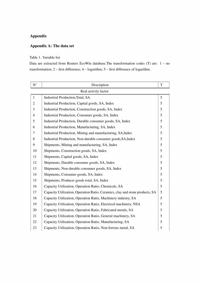
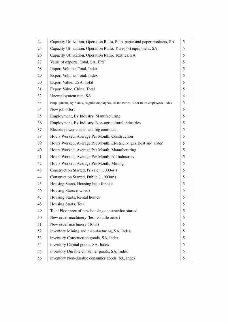
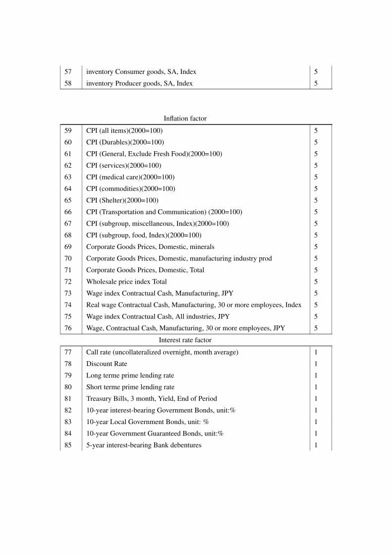
Table 1. Variable list
Data are extracted from Reuters EcoWin database.The transformation codes (T) are: 1 – no
transformation; 2 – first difference; 4 – logarithm; 5 – first difference of logarithm.
N◦ Description T
Real activity factor
1 Industrial Production,Total, SA. 5
2 Industrial Production, Capital goods, SA, Index 5
3 Industrial Production, Construction goods, SA, Index 5
4 Industrial Production, Consumer goods, SA, Index 5
5 Industrial Production, Durable consumer goods, SA, Index 5
6 Industrial Production, Manufacturing, SA, Index 5
7 Industrial Production, Mining and manufacturing, SA,Index 5
8 Industrial Production, Non-durable consumer goods,SA,Index 5
9 Shipments, Mining and manufacturing, SA, Index 5
10 Shipments, Construction goods, SA, Index 5
11 Shipments, Capital goods, SA, Index 5
12 Shipments, Durable consumer goods, SA, Index 5
13 Shipments, Non-durable consumer goods, SA, Index 5
14 Shipments, Consumer goods, SA, Index 5
15 Shipments, Producer goods total, SA, Index 5
16 Capacity Utilization, Operation Ratio, Chemicals, SA 5
17 Capacity Utilization, Operation Ratio, Ceramics, clay and stone products, SA 5
18 Capacity Utilization, Operation Ratio, Machinery industry, SA 5
19 Capacity Utilization, Operation Ratio, Electrical machinery, NSA 5
20 Capacity Utilization, Operation Ratio, Fabricated metals, SA 5
21 Capacity Utilization, Operation Ratio, General machinery, SA 5
22 Capacity Utilization, Operation Ratio, Manufacturing, SA 5
23 Capacity Utilization, Operation Ratio, Non-ferrous metal, SA 5
24 Capacity Utilization, Operation Ratio, Pulp, paper and paper products, SA 5
25 Capacity Utilization, Operation Ratio, Transport equipment, SA 5
26 Capacity Utilization, Operation Ratio, Textiles, SA 5
27 Value of exports, Total, SA, JPY 5
28 Import Volume, Total, Index 5
29 Export Volume, Total, Index 5
30 Export Value, USA, Total 5
31 Export Value, China, Total 5
32 Unemployment rate, SA 4
33 Employment, By Status, Regular employees, all industries, 30 or more employees, Index 5
34 New job offert 5
35 Employment, By Industry, Manufacturing 5
36 Employment, By Industry, Non-agricultural industries 5
37 Electric power consumed, big contracts 5
38 Hours Worked, Average Per Month, Construction 5
39 Hours Worked, Average Per Month, Electricity, gas, heat and water 5
40 Hours Worked, Average Per Month, Manufacturing 5
41 Hours Worked, Average Per Month, All industries 5
42 Hours Worked, Average Per Month, Mining 5
43 Construction Started, Private (1,000m2) 5
44 Construction Started, Public (1,000m2) 5
45 Housing Starts, Housing built for sale 5
46 Housing Starts (owned) 5
47 Housing Starts, Rental homes 5
48 Housing Starts, Total 5
49 Total Floor area of new housing construction started 5
50 New order machinery (less volatile order) 5
51 New order machinery (Total) 5
52 inventory Mining and manufacturing, SA, Index 5
53 inventory Construction goods, SA, Index 5
54 inventory Capital goods, SA, Index 5
55 inventory Durable consumer goods, SA, Index 5
56 inventory Non-durable consumer goods, SA, Index 5
57 inventory Consumer goods, SA, Index 5
58 inventory Producer goods, SA, Index 5
Inflation factor
59 CPI (all items)(2000=100) 5
60 CPI (Durables)(2000=100) 5
61 CPI (General, Exclude Fresh Food)(2000=100) 5
62 CPI (services)(2000=100) 5
63 CPI (medical care)(2000=100) 5
64 CPI (commodities)(2000=100) 5
65 CPI (Shelter)(2000=100) 5
66 CPI (Transportation and Communication) (2000=100) 5
67 CPI (subgroup, miscellaneous, Index)(2000=100) 5
68 CPI (subgroup, food, Index)(2000=100) 5
69 Corporate Goods Prices, Domestic, minerals 5
70 Corporate Goods Prices, Domestic, manufacturing industry prod 5
71 Corporate Goods Prices, Domestic, Total 5
72 Wholesale price index Total 5
73 Wage index Contractual Cash, Manufacturing, JPY 5
74 Real wage Contractual Cash, Manufacturing, 30 or more employees, Index 5
75 Wage index Contractual Cash, All industries, JPY 5
76 Wage, Contractual Cash, Manufacturing, 30 or more employees, JPY 5
Interest rate factor
77 Call rate (uncollateralized overnight, month average) 1
78 Discount Rate 1
79 Long terme prime lending rate 1
80 Short terme prime lending rate 1
81 Treasury Bills, 3 month, Yield, End of Period 1
82 10-year interest-bearing Government Bonds, unit:% 1
83 10-year Local Government Bonds, unit: % 1
84 10-year Government Guaranteed Bonds, unit:% 1
85 5-year interest-bearing Bank debentures 1
86 Government Benchmarks, 10 Year, Average 1
87 Government Benchmarks, 2 year, End of Period 1
88 Leading Index, Tokyo interbank offered rates (3 months) 1
89 Government Bond Futures Listed Yield on TSE (10 years) 1
90 Average Contracted Interest Rates on Loans and Discounts of Domestically Licensed Banks
(New)
1
91 Average Contracted Interest Rates on Loans and Discounts of Domestically Licensed Banks,
City Banks (short-term)
1
92 Average Contracted Interest Rates on Loans and Discounts of Domestically Licensed Banks,
Regional Banks (short-term)
1
93 Average Contracted Interest Rates on Loans and Discounts of Domestically Licensed Banks,
City Banks (Long-term)
1
94 Average Contracted Interest Rates on Loans and Discounts of Domestically Licensed Banks,
Regional Banks (Long-term)
1
95 Average interest rate on certificate of deposit of all banks 1
Appendix B: Estimated factors
Figure 8. Activity factor
1985 1990 1995 2000 2005
4.3
4.4
4.5
4.6
4.7
4.8
4.9
Lrgdp Lconstgoods Ldurcongd LMiningmanuf Lcaputorch Lcaputormind Lcaputorfabm Lcaputormang Lcaputorpppp Lcaputortext
Lcapital_goods Lconsgoods Lmanuf LNonduraconsgd Lcaputorccsp Lcaputorelecma Lcaputorgenm Lcaputornfmet Lcaputortrans cumfactivity
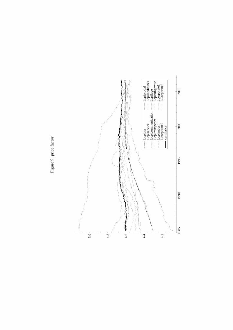
Figu
re9.
pric
efa
ctor
1985
1990
1995
2000
2005
4.2
4.4
4.6
4.8
5.0
Lcp
idur
L
cpis
ervi
ce
Lcp
icom
mun
icat
ion
Lcp
itran
spco
m
Lcp
isub
grf
Lco
rpor
ate2
cu
mfp
rice
Lcp
ipro
daf
Lcp
imed
icin
es
Lcp
iloge
L
cpis
ubgr
mis
c L
corp
orat
e1
LC
orpo
rate
3
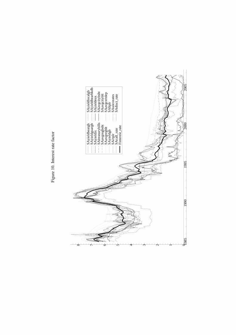
Figu
re10
.Int
eres
trat
efa
ctor
1985
1990
1995
2000
2005
012345678
SAyi
eldb
earg
b SA
yiel
dgua
rgb
SAyi
eldi
x SA
trea
sury
bills
SA
avgr
egbs
ht
SAav
greg
blt
SAyi
eldg
b SA
ctpl
r SA
call_
rate
Fi
nter
est_
rate
SAyi
eldl
ocal
gb
SAyi
eldb
earb
kdb
SAyi
elde
ux
SAav
gcity
bsht
SA
avgc
itybl
t SA
avgc
ertd
ep
SAltp
lr
SAun
cora
tes
SAdi
sct_
rate
Appendix C: MS-VAR estimation results
Table 2. Linearity test:VAR model
Lags IC Two regimesa single regime
Lag1
AIC -20.3016 -20.1844
HQ -20.1034 -20.0198
SC -19.8086 -19.7741
Lag2
AIC -20.3240 20.2545
HQ -20.0369 -20.0060
SC -19.6499 -19.6228
Lag3
AIC -20.2957 -20.1835
HQ -19.9192 -19.8402
SC -19.3593 -19.3297
aFour variable MSVAR with output, price level,
monetary base and bond yield. All information crite-
rion (values in bold font) for all number of lags support
the presence of regime shifts.
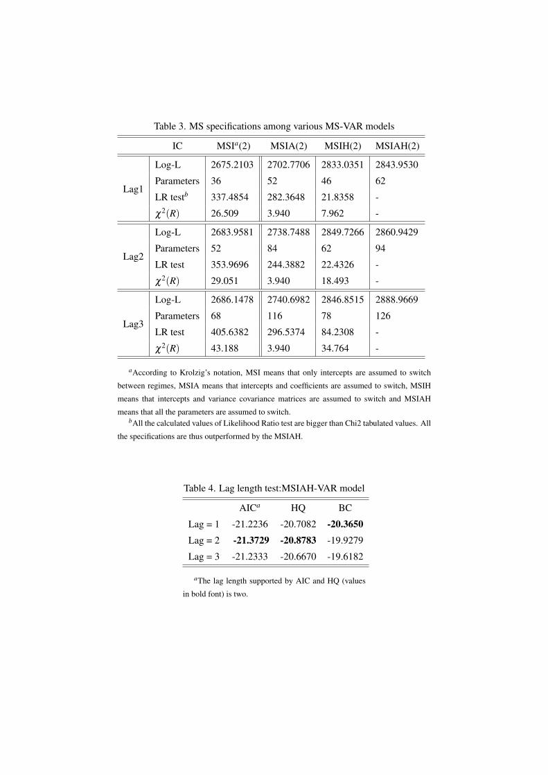
Table 3. MS specifications among various MS-VAR models
IC MSIa(2) MSIA(2) MSIH(2) MSIAH(2)
Lag1
Log-L 2675.2103 2702.7706 2833.0351 2843.9530
Parameters 36 52 46 62
LR testb 337.4854 282.3648 21.8358 -
χ2(R) 26.509 3.940 7.962 -
Lag2
Log-L 2683.9581 2738.7488 2849.7266 2860.9429
Parameters 52 84 62 94
LR test 353.9696 244.3882 22.4326 -
χ2(R) 29.051 3.940 18.493 -
Lag3
Log-L 2686.1478 2740.6982 2846.8515 2888.9669
Parameters 68 116 78 126
LR test 405.6382 296.5374 84.2308 -
χ2(R) 43.188 3.940 34.764 -
aAccording to Krolzig’s notation, MSI means that only intercepts are assumed to switch
between regimes, MSIA means that intercepts and coefficients are assumed to switch, MSIH
means that intercepts and variance covariance matrices are assumed to switch and MSIAH
means that all the parameters are assumed to switch.bAll the calculated values of Likelihood Ratio test are bigger than Chi2 tabulated values. All
the specifications are thus outperformed by the MSIAH.
Table 4. Lag length test:MSIAH-VAR model
AICa HQ BC
Lag = 1 -21.2236 -20.7082 -20.3650Lag = 2 -21.3729 -20.8783 -19.9279
Lag = 3 -21.2333 -20.6670 -19.6182
aThe lag length supported by AIC and HQ (values
in bold font) is two.
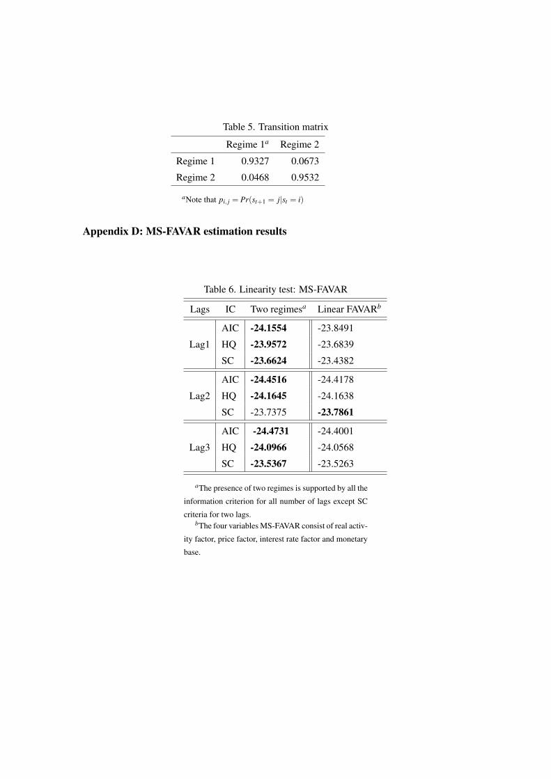
Table 5. Transition matrix
Regime 1a Regime 2
Regime 1 0.9327 0.0673
Regime 2 0.0468 0.9532
aNote that pi, j = Pr(st+1 = j|st = i)
Appendix D: MS-FAVAR estimation results
Table 6. Linearity test: MS-FAVAR
Lags IC Two regimesa Linear FAVARb
Lag1
AIC -24.1554 -23.8491
HQ -23.9572 -23.6839
SC -23.6624 -23.4382
Lag2
AIC -24.4516 -24.4178
HQ -24.1645 -24.1638
SC -23.7375 -23.7861
Lag3
AIC -24.4731 -24.4001
HQ -24.0966 -24.0568
SC -23.5367 -23.5263
aThe presence of two regimes is supported by all the
information criterion for all number of lags except SC
criteria for two lags.bThe four variables MS-FAVAR consist of real activ-
ity factor, price factor, interest rate factor and monetary
base.
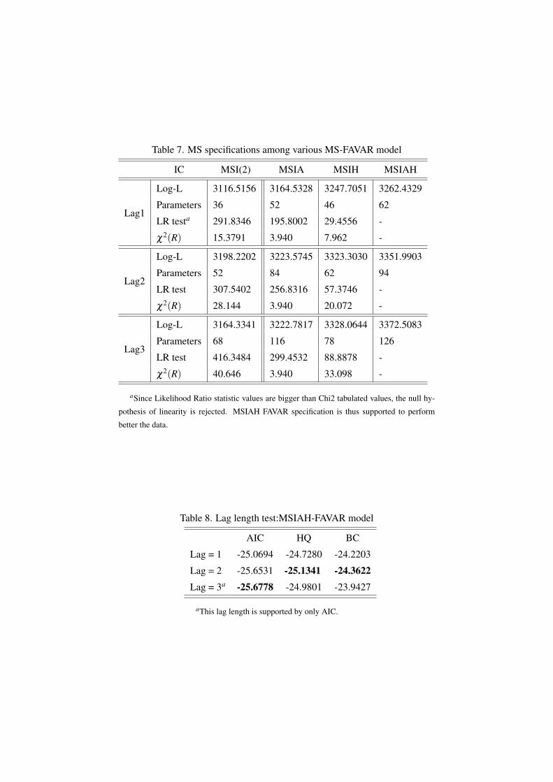
Table 7. MS specifications among various MS-FAVAR model
IC MSI(2) MSIA MSIH MSIAH
Lag1
Log-L 3116.5156 3164.5328 3247.7051 3262.4329
Parameters 36 52 46 62
LR testa 291.8346 195.8002 29.4556 -
χ2(R) 15.3791 3.940 7.962 -
Lag2
Log-L 3198.2202 3223.5745 3323.3030 3351.9903
Parameters 52 84 62 94
LR test 307.5402 256.8316 57.3746 -
χ2(R) 28.144 3.940 20.072 -
Lag3
Log-L 3164.3341 3222.7817 3328.0644 3372.5083
Parameters 68 116 78 126
LR test 416.3484 299.4532 88.8878 -
χ2(R) 40.646 3.940 33.098 -
aSince Likelihood Ratio statistic values are bigger than Chi2 tabulated values, the null hy-
pothesis of linearity is rejected. MSIAH FAVAR specification is thus supported to perform
better the data.
Table 8. Lag length test:MSIAH-FAVAR model
AIC HQ BC
Lag = 1 -25.0694 -24.7280 -24.2203
Lag = 2 -25.6531 -25.1341 -24.3622Lag = 3a -25.6778 -24.9801 -23.9427
aThis lag length is supported by only AIC.

Table 9. Transition matrix
Regime 1 Regime 2
Regime 1 0.9069 0.0333
Regime 2 0.0931 0.9667