Embed Size (px)
Citation preview

THE EFFECTS OF ADSORPTION ON INJECTION INTO
AND PRODUCTION FROM VAPOR DOMINATED
GEOTHERMAL RESERVOIRS
a dissertation
submitted to the department of petroleum engineering
and the committee on graduate studies
of stanford university
in partial fulfillment of the requirements
for the degree of
doctor of philosophy
By
John Wirt Hornbrook
January, 1994

c© Copyright 1998
by
John Wirt Hornbrook
ii

I certify that I have read this thesis and that in my opin-
ion it is fully adequate, in scope and in quality, as a
dissertation for the degree of Doctor of Philosophy.
Dr. Roland N. Horne(Principal Adviser)
I certify that I have read this thesis and that in my opin-
ion it is fully adequate, in scope and in quality, as a
dissertation for the degree of Doctor of Philosophy.
Dr. Paul Kruger
I certify that I have read this thesis and that in my opin-
ion it is fully adequate, in scope and in quality, as a
dissertation for the degree of Doctor of Philosophy.
Dr. Martin J. Blunt
Approved for the University Committee on Graduate
Studies:
iii
Abstract
An analysis was undertaken on the effects of adsorption on geothermal reservoir in-
jection performance. Thermodynamic properties of adsorbate were determined so
pressure depletion in reservoirs affected by adsorption could be modeled accurately.
A semi-analytical solution was constructed for isothermal vapor flow with a sorbing
phase present. Similarity analysis was used to isolate the effects of adsorbed mass and
the rate of change of adsorbed mass. Vapor flow in a porous medium in the presence
of a sorbing phase was solved numerically to determine the validity of the isothermal
assumption made in the analytical derivation and to study other thermal effects of
adsorption. An analysis of the heat balance for fluids flowing in geothermal systems
was used to determine the heat effects of adsorption at a boiling front and for single
phase vapor flow.
Production characteristics of an injected tritiated water tracer were studied for the
Geysers geothermal reservoir. Effects of tracer sorption, diffusion, and partitioning
were included to determine the relative importance of each effect and to explain field
tracer production characteristics.
Semi-analytical results indicate that effects of adsorption on pressure are signifi-
cant for a wide range of adsorption isotherms. The slope of the adsorption isotherm
is shown to be much more significant than the magnitude of adsorbed mass.
Numerical results indicate that the isothermal assumption is valid for vapor dom-
inated flow in geothermal reservoirs. The numerical scheme is also shown to agree
well with analytical results for a wide range of conditions.
The effects of adsorption on the propagation of injected tracer are shown to be
insignificant for a linear system. By use of stream tube modeling of a long-term tracer
iv

test at the Geysers geothermal reservoir, adsorption effects are shown not to be the
likely explanation for the observed spread in tracer production data.
v

Acknowledgements
I gratefully acknowledge the guidance I received from my advisor, Dr. Roland N.
Horne. He provided much valuable insight and helped to steer my research in the
right direction.
I thank my dissertation defense committee comprised of Dr. Paul Kruger, Dr.
Martin J. Blunt, Dr. Paul Roberts, and Dr. William E. Brigham. Special thanks go
to Dr. Kruger and Dr. Blunt for serving as readers. I also thank Dr. Brigham for
providing career and academic advice throughout my stay at Stanford.
It was an honor and a great pleasure to have worked with Dr. Henry J. Ramey,
Jr. He was a brilliant engineer and teacher and one of the nicest people I have ever
met.
My office mates, Rafael E. Guzman and Marco R. Thiele, were always available to
help me work through difficult problems, give advice, or just shoot the breeze when
I needed a break. They helped make my stay at Stanford memorable and enjoyable.
Funding for this project was provided, in part, by the Department of Energy,
Geothermal Division, under contract number DEFG0790ID12934. I gratefully ac-
knowledge their financial support.
Finally, I thank my parents, Charles and Marilyn Hornbrook, and my brother
and sister-in-law, Marc and Rosemary Hornbrook. When the research seemed like a
little too much or my finances began to run low they were always there to help. I
appreciate their support very much.
vi
Contents
Abstract iv
Acknowledgements vi
1 Introduction 1
1.1 Fundamentals of Storage and Flow in Geothermal Reservoirs . . . . . 4
1.2 Outline of Research . . . . . . . . . . . . . . . . . . . . . . . . . . . . 5
2 Thermodynamics of Geothermal Fluids 7
2.1 The Vapor Phase . . . . . . . . . . . . . . . . . . . . . . . . . . . . . 9
2.2 The Liquid Water Phase . . . . . . . . . . . . . . . . . . . . . . . . . 11
2.3 The Retained Liquid Phases . . . . . . . . . . . . . . . . . . . . . . . 11
2.3.1 Adsorbed and Capillary Retained Liquid . . . . . . . . . . . . 12
2.3.2 Density of the Retained Liquid Phases . . . . . . . . . . . . . 20
2.3.3 Thermal Properties of the Retained Liquid Phases . . . . . . . 23
2.3.4 Summary of Thermodynamic Properties . . . . . . . . . . . . 29
3 Analysis of the Energy Balance 31
3.1 Validity of Thermal Equilibrium Assumption . . . . . . . . . . . . . . 31
3.2 Effects of Adsorbed Phase on The Heat Transfer Mechanism . . . . . 33
3.3 The Energy Balance . . . . . . . . . . . . . . . . . . . . . . . . . . . 35
4 Semi-Analytical Model 39
4.1 Derivation of Analytical Solution . . . . . . . . . . . . . . . . . . . . 39
vii

4.1.1 Analysis of Adsorption Pressure Effects. . . . . . . . . . . . . 44
4.1.2 Similarity Analysis . . . . . . . . . . . . . . . . . . . . . . . . 46
4.1.3 Solution Procedure . . . . . . . . . . . . . . . . . . . . . . . . 49
4.2 Pressure Depletion Effects of an Adsorbed Phase . . . . . . . . . . . 51
4.2.1 Effects of Adsorbate Density on Pressure Depletion . . . . . . 52
5 Numerical Model 56
5.1 Single-Phase Liquid Flow Without Adsorption Effects . . . . . . . . . 58
5.2 Single-Phase Vapor Flow . . . . . . . . . . . . . . . . . . . . . . . . . 60
5.2.1 Validity of Isothermal Flow Assumption . . . . . . . . . . . . 61
5.2.2 Comparison with Analytical Solution - Adsorbed Phase Absent 63
5.2.3 Comparison with Analytical Solution - Adsorbed Phase Present 65
5.3 Modeling Tracer Response . . . . . . . . . . . . . . . . . . . . . . . . 67
5.3.1 Effects of Adsorption on Tracer Propagation . . . . . . . . . . 68
5.3.2 Effects of Diffusion Partitioning on Tracer Propagation . . . . 82
5.3.3 Effects of Preferential Partitioning on Tracer Propagation . . . 88
6 The Geysers Geothermal Reservoir 90
6.1 Geysers Reservoir Properties . . . . . . . . . . . . . . . . . . . . . . . 93
6.2 Injection at the Geysers . . . . . . . . . . . . . . . . . . . . . . . . . 95
6.2.1 History of Injection at the Geysers . . . . . . . . . . . . . . . 97
6.2.2 Effects of Injection on Adsorbate Recharge . . . . . . . . . . . 105
6.3 Tracer Studies at the Geysers . . . . . . . . . . . . . . . . . . . . . . 106
6.3.1 Effects of Adsorption on Geysers Tracer Tests . . . . . . . . . 106
7 Conclusions 116
Nomenclature 119
References 123
A Computational Data 131
viii

B Computer Programs 137
ix

List of Tables
2.1 Density Variation Between Condensed and Saturated Liquid Phases . 21
3.1 Thermal Diffusivity of Water . . . . . . . . . . . . . . . . . . . . . . . 38
5.1 Thermal Effects of Adsorbed Phase . . . . . . . . . . . . . . . . . . . 64
6.1 Geysers Reservoir Properties . . . . . . . . . . . . . . . . . . . . . . . 94
6.2 Well Production Data . . . . . . . . . . . . . . . . . . . . . . . . . . 108
6.3 OS-23 Stream tube data. . . . . . . . . . . . . . . . . . . . . . . . . . 112
A.1 Well OS-23 Tracer Production Data . . . . . . . . . . . . . . . . . . . 132
x

List of Figures
2.1 Fluid distributions in a geothermal porous medium . . . . . . . . . . 7
2.2 Vapor phase pressure lowering (after Udell [66]) . . . . . . . . . . . . 11
2.3 Geysers pore cumulative volume vs. pore radius (from Micromeritics
[37]) . . . . . . . . . . . . . . . . . . . . . . . . . . . . . . . . . . . . 15
2.4 Liquid phase pressure lowering (after Udell [66]) . . . . . . . . . . . . 17
2.5 Geysers adsorption isotherm at 120 ◦C (after Shang [65]) . . . . . . . 18
2.6 Geysers liquid saturation with constant liquid density. . . . . . . . . . 19
2.7 Specific volume of saturated water . . . . . . . . . . . . . . . . . . . . 20
2.8 Retained liquid density as a function of pressure (Geysers sample) . . 22
2.9 Geysers liquid saturation with variable liquid density. . . . . . . . . . 23
2.10 Rate of change of radius with respect of volume (Geysers sample) . . 25
2.11 Surface extension effects on the heat of vaporization . . . . . . . . . . 26
2.12 Liquid compression effects on the heat of vaporization . . . . . . . . . 27
2.13 Pore drying effects on the heat of vaporization . . . . . . . . . . . . . 28
2.14 Effects of pore size and temperature on the heat of vaporization . . . 29
3.1 Time required for thermal equilibration of injected fluid . . . . . . . . 34
4.1 Compressibility of steam at 200 C . . . . . . . . . . . . . . . . . . . . 42
4.2 Compressibility of steam at 300 C . . . . . . . . . . . . . . . . . . . . 43
4.3 Langmuir isotherms for a range of shape factors, c . . . . . . . . . . . 45
4.4 Size of the mass rate of change term in the nonlinear term . . . . . . 46
4.5 Similarity function for a range of adsorption isotherms . . . . . . . . 49
4.6 Early time depletion effects of adsorption . . . . . . . . . . . . . . . . 52
xi

4.7 Late time depletion effects of adsorption . . . . . . . . . . . . . . . . 54
4.8 Comparison with Geysers isotherm . . . . . . . . . . . . . . . . . . . 54
4.9 Comparison with Geysers isotherm (early time) . . . . . . . . . . . . 55
4.10 Comparison with Geysers isotherm (late time) . . . . . . . . . . . . . 55
5.1 Pressure histories for constant compressibility flow. . . . . . . . . . . 60
5.2 Vapor pressure histories under different thermal conditions. . . . . . . 62
5.3 Analytical and numerical solutions with no adsorption . . . . . . . . 65
5.4 Analytical and numerical solutions with constant adsorption . . . . . 66
5.5 Analytical and numerical solutions with Langmuir adsorption . . . . 67
5.6 Schematic of numerical core with tracer in vapor phase. . . . . . . . . 71
5.7 Tracer production histories with tracer in vapor phase. . . . . . . . . 71
5.8 Tracer production histories with tracer in vapor phase. . . . . . . . . 72
5.9 Schematic of numerical core with tracer in adsorbed phase. . . . . . . 73
5.10 Tracer production histories with tracer in adsorbed phase. . . . . . . 74
5.11 Tracer profiles for steady state conditions. . . . . . . . . . . . . . . . 75
5.12 Tracer profiles for transient conditions. . . . . . . . . . . . . . . . . . 76
5.13 Tracer production for early initiation of injector. . . . . . . . . . . . . 78
5.14 Tracer production for midlife injection initiation. . . . . . . . . . . . . 79
5.15 Tracer production for late initiation of injector. . . . . . . . . . . . . 80
5.16 Tracer production from injector (pi = 8 MPa). . . . . . . . . . . . . . 80
5.17 Tracer production from injector (pi = 4 MPa). . . . . . . . . . . . . . 81
5.18 Tracer production from injector (pi = 0.101 MPa). . . . . . . . . . . . 81
5.19 Schematic of porosity in a geothermal reservoir. . . . . . . . . . . . . 83
5.20 Pressure profiles for diffusion tracer delay. . . . . . . . . . . . . . . . 87
6.1 Location of the Geysers geothermal field (from Koenig [38]) . . . . . 91
6.2 Geysers production (from Barker, et. al. [7]) . . . . . . . . . . . . . . 92
6.3 Unit location at the Geysers (from Barker, et. al. [7]) . . . . . . . . . 98
6.4 LPA well locations (from Enedy, et. al. [22]) . . . . . . . . . . . . . . 101
6.5 F-4 observation well pressures (from Enedy, et. al. [22]) . . . . . . . . 102
6.6 LPA monthly flowrate (from Enedy, et. al. [22]) . . . . . . . . . . . . 103
xii

6.7 Schematic of well placement for streamline generation. . . . . . . . . 109
6.8 DX-8 tracer study streamlines. . . . . . . . . . . . . . . . . . . . . . . 109
6.9 Streamlines for DX-8/OS-23 well pair. . . . . . . . . . . . . . . . . . 110
6.10 Tritium production from OS-23 (from UNOCAL [67]) . . . . . . . . . 113
6.11 Mass concentration of produced tritium (from UNOCAL [67]) . . . . 114
6.12 Mass concentration of producted tritium (stream tube model) . . . . 115
A.1 Gas law deviation factors for steam. . . . . . . . . . . . . . . . . . . . 131
xiii

Chapter 1
Introduction
In the current era of environmental awareness, geothermal energy represents an excel-
lent and significant alternative to conventional energy resources. With increasingly
strict clean air standards and concern over the long term effects of pollution from
fossil fuels, geothermal exploration and development has been increasing. Reed and
McLarty [48] estimated that, as of 1992, geothermal resources accounted for about 1
billion dollars of annual revenue and displaced over 30 million barrels of imported oil.
They also estimated that about 7 % of the electrical energy needs in California were
met by geothermal sources.
In addition to the United States, significant geothermal development has taken
place in the Philippines, Mexico, Italy, New Zealand, and Japan. Most U.S. develop-
ment has taken place in the western states with 18 resource sites currently operating
in California, Nevada, and Utah, accounting for over 2700 MW of electrical generation
capacity.
Geothermal reservoirs may be described as vapor-dominated, liquid-dominated,
or hot dry rock reservoirs. Vapor-dominated geothermal reservoirs are characterized
by low pressures and high temperatures which requires that all or most of the resident
fluid is in the form of superheated or saturated steam. Electrical generation from the
reservoirs is accomplished by simply producing steam into conventional turbines to
drive electrical generators.
At somewhat lower temperatures are liquid-dominated geothermal reservoirs. In
1

CHAPTER 1. INTRODUCTION 2
these systems most of the resident fluid is in the form of liquid. Electrical generation is
accomplished either by partially flashing the produced water to steam for subsequent
flow through turbines, or by using heat from the produced water to vaporize a more
volatile liquid and using the generated vapor to power turbines.
Hot dry rock geothermal reservoirs consist of high temperature rock bodies with
insufficient liquid flow to carry the heat to the surface. Injection of water into arti-
ficially induced fractures to produce steam for electrical generation is the method of
heat extraction in these systems.
This research focuses on vapor-dominated reservoirs. Specifically, the Geysers
geothermal reservoir, the largest developed geothermal steam resource in the world,
was studied to determine the effects of adsorption on injection into this type of
geothermal reservoir. Methods generally applied to oil and gas reservoirs were used
to determine the characteristics of geothermal reservoirs when an adsorbed phase is
present.
As in oil and gas reservoirs, the fluids in geothermal reservoirs are depletable.
The difference between depletion of petroleum and geothermal reservoirs is that the
energy usually is not depleted from geothermal reservoirs even when all the fluid has
been produced. The energy stored in geothermal reservoirs is in the form of heat,
and, due to the high heat capacity and total mass of the formation itself, most of the
heat stored in geothermal reservoirs cannot be removed under primary production.
It is common, therefore, to inject produced water back into the reservoir to maximize
the energy extraction.
To design effective injection and production programs for geothermal reservoirs,
the physics of the flow in the reservoirs must be understood. However, understanding
this flow is not an easy task. Geothermal reservoirs are, in general, highly fractured
and heterogeneous, and the transport of fluids is influenced strongly by heat diffusion
and by the presence of liquid retained in the porous matrix which acts as a mass
source for the produced fluids. This retained liquid may be in the form of capillary
condensed water or liquid adsorbed onto the rock grains.
The first stage in understanding the physics of flow in geothermal reservoirs is
to understand the isothermal flow of fluids in porous and fractured media. The

CHAPTER 1. INTRODUCTION 3
petroleum engineering literature is replete with analyses of this subject.
The second stage in understanding flow in geothermal systems is to understand the
simultaneous transport of fluid and heat in porous media. Beginning with the work of
Whiting and Ramey [71], numerous researchers have studied transport and storage in
geothermal reservoirs. Crank [17] presented a mathematical analysis of the simulta-
neous diffusion of pressure and heat. Brigham and Morrow [12] applied gas reservoir
volumetric analysis to geothermal reservoirs with excellent results. Herkelrath, et. al.
[34] and Moench and Atkinson [49] presented models for the simultaneous diffusion
of fluid and heat in one dimensional systems and matched experimental data. Pruess,
et. al. [56] presented an analytical solution for heat transfer at a boiling front, while
Fitzgerald and Woods [24], Fitzgerald and Woods [25], Woods and Fitzgerald [73],
and Doughty and Pruess [20] presented similarity solutions describing the flow of
water, vapor, and heat in geothermal reservoirs. Pruess [55] studied heat transfer at
the boiling front and Pruess and Narasimhan [57] considered flow in fractured vapor-
dominated reservoirs. All of the research described above assumed no retained liquid
phase. Thus, in much research carried out on fluid and mass transfer, an important
element is missing.
The third stage in understanding flow in geothermal systems is to understand the
effects of retained liquid on the flow of fluids and heat in porous media. Retained
liquid (adsorption) effects have been studied for a number of vapor storage systems.
Lin and Ma [42], Bojan, et. al. [10], and Pogorelov and Churmayev [54] provided
theoretical analyses of adsorption in an array of porous media. Blazek, et. al. [9]
studied the effects of adsorption in methane storage tanks. Morrow [50], Schettler,
et. al. [63], Lane, et. al. [39], and Calson and Mercer [14] studied the effects of
gas adsorption in low permeability gas reservoirs. Hawkins, et. al. [33], Anbarci
and Ertekin [4], Nguyen [53], Matranga, et. al. [43], Matranga, et. al. [44], Bhatia
[8], and McElhiney, et. al. [47] studied the effects of adsorption in coal-bed methane
reservoirs. The research listed above shows that in methane storage systems, coal-bed
methane reservoirs, and low permeability gas reservoirs, adsorption of vapor can play
a major role on the storage and pressure depletion characteristics in these systems.
For geothermal reservoirs, the same systematic analysis of adsorption effects is not
CHAPTER 1. INTRODUCTION 4
yet complete.
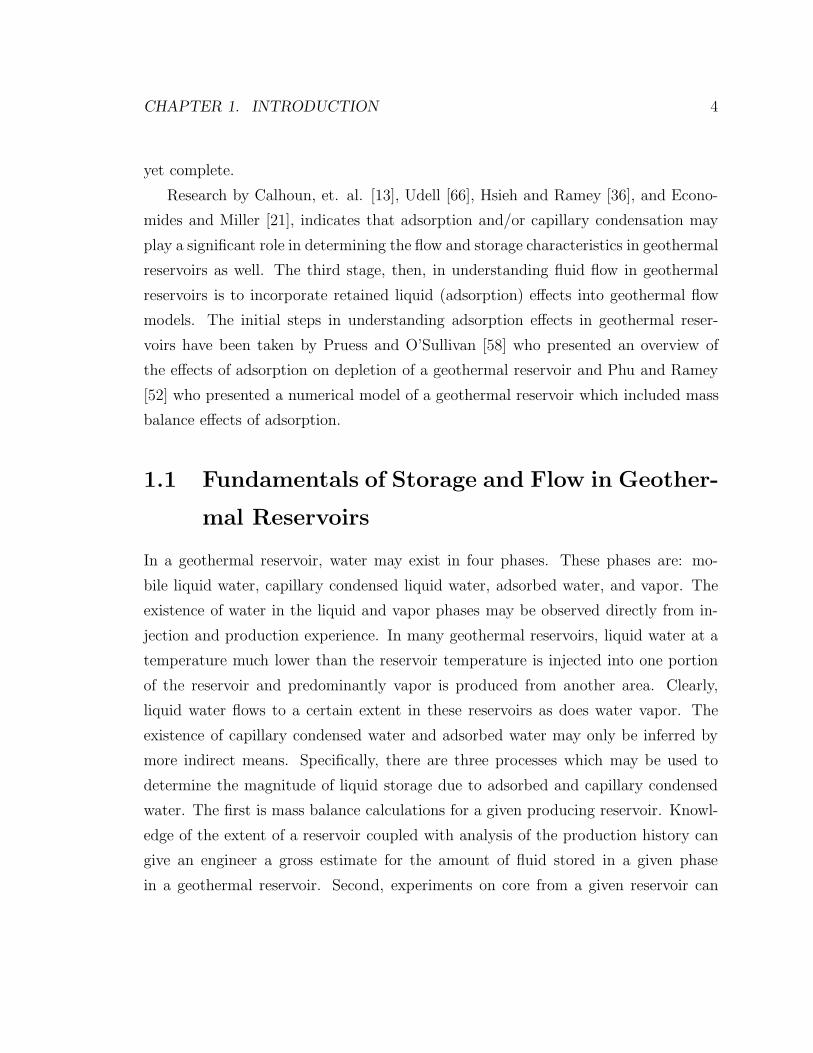
Research by Calhoun, et. al. [13], Udell [66], Hsieh and Ramey [36], and Econo-
mides and Miller [21], indicates that adsorption and/or capillary condensation may
play a significant role in determining the flow and storage characteristics in geothermal
reservoirs as well. The third stage, then, in understanding fluid flow in geothermal
reservoirs is to incorporate retained liquid (adsorption) effects into geothermal flow
models. The initial steps in understanding adsorption effects in geothermal reser-
voirs have been taken by Pruess and O’Sullivan [58] who presented an overview of
the effects of adsorption on depletion of a geothermal reservoir and Phu and Ramey
[52] who presented a numerical model of a geothermal reservoir which included mass
balance effects of adsorption.
1.1 Fundamentals of Storage and Flow in Geother-
mal Reservoirs
In a geothermal reservoir, water may exist in four phases. These phases are: mo-
bile liquid water, capillary condensed liquid water, adsorbed water, and vapor. The
existence of water in the liquid and vapor phases may be observed directly from in-
jection and production experience. In many geothermal reservoirs, liquid water at a
temperature much lower than the reservoir temperature is injected into one portion
of the reservoir and predominantly vapor is produced from another area. Clearly,
liquid water flows to a certain extent in these reservoirs as does water vapor. The
existence of capillary condensed water and adsorbed water may only be inferred by
more indirect means. Specifically, there are three processes which may be used to
determine the magnitude of liquid storage due to adsorbed and capillary condensed
water. The first is mass balance calculations for a given producing reservoir. Knowl-
edge of the extent of a reservoir coupled with analysis of the production history can
give an engineer a gross estimate for the amount of fluid stored in a given phase
in a geothermal reservoir. Second, experiments on core from a given reservoir can

CHAPTER 1. INTRODUCTION 5
yield actual measurements of the adsorbed and capillary condensed phases. The rel-
ative amounts of adsorbate and capillary condensed phase may also be deduced from
experimental results as will be discussed in Chapter 2. Third, an application of the
physics of capillary behavior may be used to determine whether a capillary condensed
phase or an adsorbed phase is present for a given range of pore sizes. When used to-
gether, the three processes described above can provide a better understanding of the
distributions, thermodynamics, and relative amounts of the adsorbed and capillary
condensed phases present.
Accurate determination of the characteristics and relative amounts of each of the
phases present in geothermal reservoirs is of paramount importance to understand
flow in these reservoirs.
Despite the extensive research directed at flow in geothermal reservoirs, no gener-
ally applicable determination of adsorptive effects has yet been presented. Most of the
previous work has focused on specific reservoirs or has been carried out by numerical
means under very specific conditions. There is a need, therefore, to determine, in a
general way, the effects of a retained liquid phase on the pressure response and flow
characteristics in geothermal reservoirs. This research develops that general approach
and applies it to flow in the Geysers geothermal reservoir.
1.2 Outline of Research
To meet the overall objectives, the research was performed in several sections:
1. Thermodynamics of Geothermal Fluids. Thermodynamic properties of
adsorbed and capillary condensed liquid were studied in detail to determine their
properties for subsequent modeling. At present, there is some confusion as to
the differences, if any, between adsorbed and condensed phases. In this section,
differences between the two phases were explained. Quantitative conclusions
were drawn as to the relative volumes of adsorbed and capillary condensed fluids
at the Geysers and the implications for fluid thermodynamics were examined.

CHAPTER 1. INTRODUCTION 6
2. Analysis of the Energy Balance. One method of extending the producing
life of a geothermal reservoir is to inject surface water into the reservoir to
replace produced mass. It is unclear whether a retained liquid phase plays a
significant role in the propagation of the boiling liquid front or if it affects the
heat transfer in the reservoir. In this section, a dimensional analysis of heat
effects was carried out to determine heat effects of a retained liquid phase.
3. Semi-Analytical Model. Adsorbed liquid mass as a function of pressure is
available in the form of adsorption isotherms. A straightforward method of
determining the effects of this adsorbed mass on pressure would allow simple
determination of adsorption effects. An analytical solution was derived for
single-phase vapor flow in the presence of a retained liquid phase.
4. Numerical Model. To model tracer production characteristics and to check
thermal assumptions not easily modeled analytically, a numerical solution is
needed. A one-dimensional implicit pressure, explicit saturation and tempera-
ture finite difference model was developed to model vapor flow in the presence
of an adsorbed phase.
5. The Geysers Geothermal Reservoir. In an attempt to track injected fluids
and to infer reservoir characteristics, tracer is often injected into geothermal
reservoirs along with recharge fluids. Unfortunately, due to the complicated
nature of the tracer production histories, interpretation is often difficult. The
purpose of this section was to determine the role of retained liquids on the pro-
duction history of injected tracer. Tracer histories from the Geysers geothermal
reservoir were modeled and conclusions were reached about the importance of
several factors in the propagation of tracer.

Chapter 2
Thermodynamics of Geothermal
Fluids
Before flow in geothermal reservoirs can be comprehensively analyzed, the different
fluid phases must be defined and their thermodynamics understood. The fluids stud-
ied are free liquid, free vapor, capillary condensed liquid, and adsorbed liquid. When
all four fluid phases are present in a geothermal reservoir, fluid distributions are as
shown schematically in Figure 2.1.
AAAAAAAAAAAAAAAAAAAAAAAAAAAAAAAAAAAA
AAAAAAAAAAAAAA
AAAAAAAAAAAAAAAA
AAAAAAAAAAAAAAAA
AAAAAAAAAAAAAAAAAAAAAAAAAAAAAAAAAAAAAAAAAAAAAAAAAAAAAAAAAAAAAAAAAAAAAAAAAAAAAA
AAAA Vapor
Liquid Water
AAAAAAAA
Condensed Water
Adsorbed Water
10-8 mRock
Figure 2.1: Fluid distributions in a geothermal porous medium
7
CHAPTER 2. THERMODYNAMICS OF GEOTHERMAL FLUIDS 8
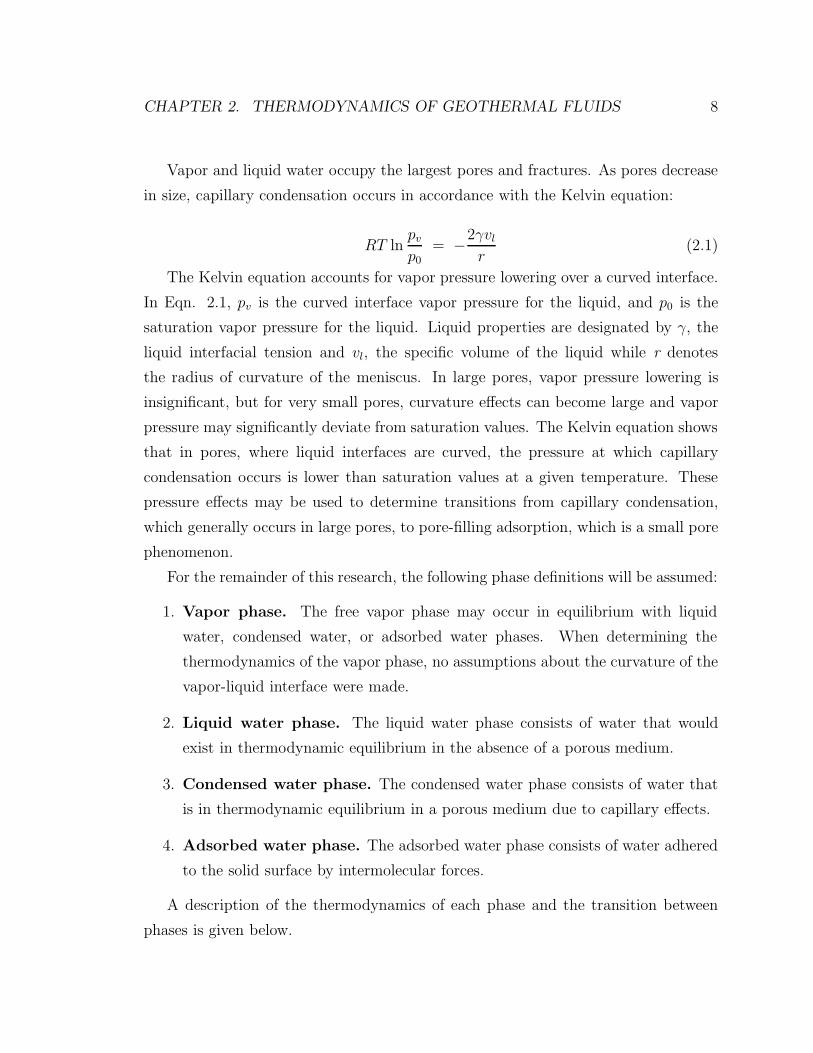
Vapor and liquid water occupy the largest pores and fractures. As pores decrease
in size, capillary condensation occurs in accordance with the Kelvin equation:
RT lnpv
p0= −2γvl
r(2.1)
The Kelvin equation accounts for vapor pressure lowering over a curved interface.
In Eqn. 2.1, pv is the curved interface vapor pressure for the liquid, and p0 is the
saturation vapor pressure for the liquid. Liquid properties are designated by γ, the
liquid interfacial tension and vl, the specific volume of the liquid while r denotes
the radius of curvature of the meniscus. In large pores, vapor pressure lowering is
insignificant, but for very small pores, curvature effects can become large and vapor
pressure may significantly deviate from saturation values. The Kelvin equation shows
that in pores, where liquid interfaces are curved, the pressure at which capillary
condensation occurs is lower than saturation values at a given temperature. These
pressure effects may be used to determine transitions from capillary condensation,
which generally occurs in large pores, to pore-filling adsorption, which is a small pore
phenomenon.
For the remainder of this research, the following phase definitions will be assumed:
1. Vapor phase. The free vapor phase may occur in equilibrium with liquid
water, condensed water, or adsorbed water phases. When determining the
thermodynamics of the vapor phase, no assumptions about the curvature of the
vapor-liquid interface were made.
2. Liquid water phase. The liquid water phase consists of water that would
exist in thermodynamic equilibrium in the absence of a porous medium.
3. Condensed water phase. The condensed water phase consists of water that
is in thermodynamic equilibrium in a porous medium due to capillary effects.
4. Adsorbed water phase. The adsorbed water phase consists of water adhered
to the solid surface by intermolecular forces.
A description of the thermodynamics of each phase and the transition between
phases is given below.

CHAPTER 2. THERMODYNAMICS OF GEOTHERMAL FLUIDS 9
2.1 The Vapor Phase
When liquid water is present in a geothermal reservoir, all small pores are occupied by
either adsorbed or condensed phases which leaves only the largest pores, those unaf-
fected by capillary effects, to be filled with liquid water and vapor. Thus, when liquid
water is present, flat surface thermodynamics are valid for the vapor phase. When
liquid water is not present and the vapor phase interfaces directly with either the con-
densed or adsorbed phase, thermodynamics of the vapor phase are altered somewhat
from standard flat-surface values. Udell [66] showed that for a given temperature, the
effective pressure lowering in the liquid and vapor phases may be calculated.
The pressure difference between liquid and vapor phases across a curved interface
is given by:
pv − pl =2γ
re(2.2)
where the effective pore radius is given by:
re =r
cos θ(2.3)
Udell [66] showed that, in a porous medium, both the vapor and the liquid exist in
a superheated state. Therefore, in a porous medium, the physical and thermodynamic
properties of both vapor and liquid differ from their properties in the absence of a
porous medium. By equating the chemical potentials of the two phases (which is
necessary for thermodynamic equilibrium) it is possible to derive an expression for
vapor pressure lowering in the system. The chemical potential, µ for vapor phase
may be written as:
µv = µ0 −∫ p0
pv
vvdp (2.4)
and, assuming the vapor specific volume, vv may be written in terms of the ideal gas
law, Eqn. 2.4 may be written as,
µv = µ0 − RT lnp0
pv(2.5)

CHAPTER 2. THERMODYNAMICS OF GEOTHERMAL FLUIDS 10
Analogous to the chemical potential balance for the vapor phase, the liquid phase
potential balance is written:
µl = µ0 −∫ p0
pl
vldp (2.6)
and, if the liquid phase is assumed incompressible, Eqn. 2.6 may be rewritten as,
µl = µ0 − (p0 − pl)vl (2.7)
For thermodynamic equilibrium, the chemical potentials in the liquid and vapor
phases must be equal. Thus, by equating the expressions obtained in Eqns. 2.5 and
2.7 and substituting Eqn. 2.2, the following expression for the vapor pressure lowering
is obtained:
2γ
re= RTρl ln
po
pv− (po − pv) (2.8)
Eqn. 2.8 is analogous to the Kelvin equation and is equivalent when the saturation
pressure, po, is equal to the pressure in the vapor phase, pv. As will be shown, this
assumption is usually a good one. It is noted that the Kelvin equation in its common
form, Eqn. 2.1 makes the assumption that pressure lowering in the vapor phase is
small. Eqn. 2.8 does not make that assumption a priori. Thus, it is possible to
investigate the effects of the presence of a porous medium on the properties of the
vapor phase.
For the range of pore sizes in which vapor is likely to occur, vapor pressure lowering
is quite small. Udell [66] reported that, for radii greater than 0.1 µm, vapor pressure
lowering is less than 0.1 percent. Figure 2.2 shows pressure lowering in the vapor phase
for a range of temperatures and pore sizes. The ordinate in Figure 2.2 is written as
the deviation from saturation pressure. Each curve endpoint corresponds to the point
at which Eqn. 2.8 predicts a liquid pressure of 0 (this result will be explained in detail
later). Based on results shown in Figure 2.2, vapor thermodynamics may be assumed
to be flat surface thermodynamics regardless of fluid saturation with very little loss
of accuracy.

CHAPTER 2. THERMODYNAMICS OF GEOTHERMAL FLUIDS 11
10-6
10-5
10-4
10-3
10-2
10-1
1
(po -
pv)
/ po
10-9 10-8 10-7 10-6 10-5 10-4
re (m)
100 C
200 C
300 C
Figure 2.2: Vapor phase pressure lowering (after Udell [66])
Steam properties tabulated by the National Institute of Standards and Technology
(NIST) [26] were used in this research for vapor properties.
2.2 The Liquid Water Phase
By definition, the liquid water phase is the water phase which is unaffected by capillary
curvature. Thus, if a flowing liquid phase is present, the thermodynamics of that phase
may be determined from standard thermodynamic tables. In all the calculations made
here, it was assumed that the liquid water phase was pure water with no dissolved
salts.
2.3 The Retained Liquid Phases
To model the flow of fluids in the presence of a condensed or adsorbed phase (re-
tained liquid phase), a minimum of two characteristics of the adsorbed fluids must be
known. First, a relationship between system pressure and mass of adsorbate must be
known. This information is determined by adsorption isotherms and by estimates of

CHAPTER 2. THERMODYNAMICS OF GEOTHERMAL FLUIDS 12
the adsorbate density. Second, knowledge of the internal energy and heat of adsorp-
tion (condensation) is necessary to accurately model heat effects of fluid flow in the
presence of an adsorbing (condensing) phase.
No thermodynamic tables of retained water phase exist, and it is unlikely that
any tables will ever be compiled since liquid retention characteristics are matrix de-
pendent. Thus, to determine thermodynamics of the adsorbed phase, it is necessary
to make inferences from measurable quantities in a given porous medium.
2.3.1 Adsorbed and Capillary Retained Liquid
In 1968, Ramey [59] showed that, in the Geysers geothermal reservoir, the volume of
the reservoir was too small to store all of its mass as water vapor. In other words,
even though all production from the Geysers had been vapor, the fluid must be
stored as water in the reservoir. This conclusion led to the paradox that liquid water
must exist in the Geysers reservoir at a pressure and temperature at which liquid
water can not exist under normal conditions. The “paradox of the Geysers” led
numerous authors, among them White [70] to speculate that either a separate liquid
water source, external to the vapor dominated reservoir, is responsible for recharge
in the Geysers, or storage in the Geysers is accomplished by capillary retained or
adsorbed water which, due to vapor-pressure lowering may exist as a liquid under
conditions which would normally specify vapor. Subsequent research has failed to
find any evidence of a hidden water source recharging the Geysers while a number
of investigations have shown retention of water within the reservoir itself to be the
most plausible mass storage source. It is, however, the way that this fluid is stored
and the effects of the the storage that have yet to be fully characterized.
In 1941, Leverett [41] discussed the principles of capillarity and defined the term
“capillary pressure” as the difference in pressure between the wetting and non-wetting
phases in a porous medium. During the following years, several authors presented
experimental and theoretical analyses of capillary pressure effects under a number of
conditions. It was the desire of Calhoun [13], et. al. [13] in 1949 to “amplify” existing
capillary pressure correlations by extending measurements to systems with very low

CHAPTER 2. THERMODYNAMICS OF GEOTHERMAL FLUIDS 13
liquid saturations and by expanding the range of liquids studied. Calhoun [13] pre-
sented a series of measurements of vapor pressure lowering and capillary pressure as
a function of water saturation and showed that vapor pressure lowering may be very
significant in small pores. Since Calhoun’s [13] measurements extend to extremely
low water saturations, they seem to indicate that capillary condensation is the sole
mechanism for vapor pressure lowering in porous media. However, Hsieh and Ramey
[35] pointed out in 1978 that at low liquid saturations, the vapor pressure lowering
reported by Calhoun [13] was actually due to adsorption rather than to capillary
effects. Hsieh and Ramey [35] defined a theoretical limit to vapor condensation to
correspond to a pore of radius equal to the radius of a water molecule. This min-
imum pore radius as defined by Hsieh and Ramey [35] is 2 A. By calculating the
vapor pressure lowering expected in a pore of this size, they defined a maximum va-
por pressure lowering due to capillary retention. Many of Calhoun’s [13] reported
values of vapor pressure lowering were actually greater than the maximum possible
reported by Hsieh and Ramey [35], thus leading to the conclusion that, for a given
porous medium, saturation below a certain point is controlled by adsorption rather
than capillary condensation.
Subsequent work has focused on accurate determination of the pore size at which
adsorption becomes the dominant process in pore filling. In 1982, Ramsay and Booth
[60] measured pore sizes in oxide sols and gels by neutron scattering and nitrogen
adsorption. By comparing measured fluid volumes and pore sizes, they concluded
that the transition radius at which adsorption pore filling begins is 1.4 nm (14 A).
In 1986, Evans et. al. [23] showed that the transition from adsorption to capillary
condensation is not accurately modeled by the Kelvin equation. They showed that
the influence of the solid surface and the small confining volume on fluid properties
may strongly affect the accuracy of the Kelvin equation below 2 nm (20 A). In 1990,
Ramsay and Wing [61] measured water vapor sorption in porous silica and ceria gels
by both a mass approach, and by neutron scattering methods. They were able to
show that in microporous solids, pore filling adsorption of water vapor commences at
pore radii of about 3.5 nm (35 A). The experiments were carried out at 150 ◦C so
they are directly applicable to geothermal systems. Experiments in mesoporous solids

CHAPTER 2. THERMODYNAMICS OF GEOTHERMAL FLUIDS 14
indicated that single and multi-layer adsorption are important in pores of radius as
large as 12 nm (120 A).
So, measurement of fluid distributions of adsorbed and capillary condensed fluids
are available in a variety of porous materials. These measurements may be used as
an aid in determining the likely fluid distributions in geothermal reservoirs. However,
direct measurement of fluid saturations and pore size distributions in geothermal
reservoirs are necessary to accurately determine the relative amounts of adsorbed
and capillary condensed liquids in these reservoirs.
In 1981, in an early attempt to determine the amount of adsorbed liquid in geother-
mal reservoirs, Hsieh and Ramey [36] showed that in many dry steam geothermal
reservoirs, surface adsorption may be the most important mechanism in vapor pres-
sure lowering and mass storage. They also found adsorption to be a significant stor-
age mechanism in geothermal reservoirs and, under certain conditions, in natural gas
reservoirs. Their work was carried out in consolidated and unconsolidated sandstone
so it was not directly applicable to geothermal reservoirs.
Direct measurement of adsorption/capillary retention in the Geysers reservoir has
been carried out by Shang and Horne [64] and Micromeritics Instrument Corpora-
tion [37]. In a series of experiments designed to measure the mass storage effects of
adsorption and the effects of temperature on adsorption, Shang and Horne [64] have
presented a number of measurements of liquid retention in Geysers geothermal core
material. In consideration of reported adsorption isotherms, simple reasoning leads to
the conclusions that at a zero pressure, liquid retention is at a minimum for a given
porous medium and is often zero. At a pressure just greater than the saturation
pressure, the sample must be at 100 % liquid saturation. Finally, at the saturation
pressure, the saturations of liquid and vapor are determined by flat surface thermo-
dynamics. Since it is known that both adsorption and capillary condensation occur
in a porous medium, the “adsorption” isotherm must contain information on both
the adsorbed amount and the capillary condensed amount between relative pressures
of zero and one. (Adsorption isotherms are commonly reported in terms of “relative
pressure” which is the system pressure divided by the saturation pressure). In fact,
Correa [64] showed that an “adsorption” isotherm may be created by combining the
CHAPTER 2. THERMODYNAMICS OF GEOTHERMAL FLUIDS 15
theoretical saturation vs. pressure data of adsorbed and capillary condensed liquid.
Thus, from a saturation standpoint, an adsorption isotherm may be considered as
an adsorbate/condensate isotherm containing information about both an adsorbed
phase and a condensed phase.
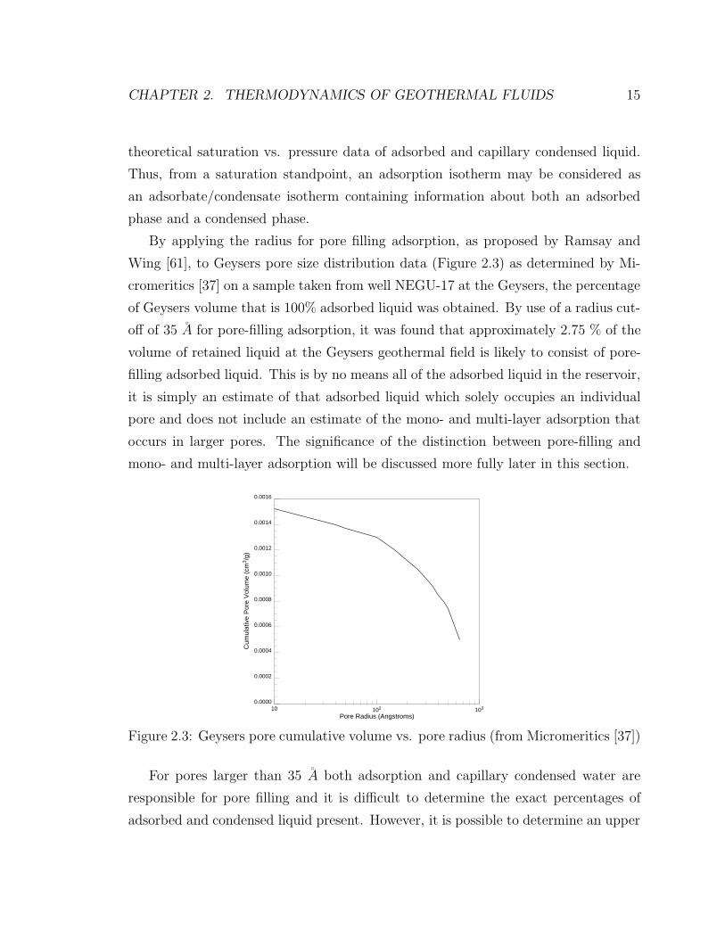
By applying the radius for pore filling adsorption, as proposed by Ramsay and
Wing [61], to Geysers pore size distribution data (Figure 2.3) as determined by Mi-
cromeritics [37] on a sample taken from well NEGU-17 at the Geysers, the percentage
of Geysers volume that is 100% adsorbed liquid was obtained. By use of a radius cut-
off of 35 A for pore-filling adsorption, it was found that approximately 2.75 % of the
volume of retained liquid at the Geysers geothermal field is likely to consist of pore-
filling adsorbed liquid. This is by no means all of the adsorbed liquid in the reservoir,
it is simply an estimate of that adsorbed liquid which solely occupies an individual
pore and does not include an estimate of the mono- and multi-layer adsorption that
occurs in larger pores. The significance of the distinction between pore-filling and
mono- and multi-layer adsorption will be discussed more fully later in this section.
0.0000
0.0002
0.0004
0.0006
0.0008
0.0010
0.0012
0.0014
0.0016
Cum
ulat
ive
Por
e V
olum
e (c
m3/g
)
10 102 103
Pore Radius (Angstroms)
Figure 2.3: Geysers pore cumulative volume vs. pore radius (from Micromeritics [37])
For pores larger than 35 A both adsorption and capillary condensed water are
responsible for pore filling and it is difficult to determine the exact percentages of
adsorbed and condensed liquid present. However, it is possible to determine an upper

CHAPTER 2. THERMODYNAMICS OF GEOTHERMAL FLUIDS 16
limit on pore size for which adsorption is likely to occur.
Udell [66] pointed out that when capillary condensation occurs in a porous medium,
both liquid and vapor exist in a superheated state which changes the shape of the
two phase region and results in the existence of both the liquid and vapor phases
at pressures lower than predicted by flat surface thermodynamics. The combination
of Eqns. 2.8 and 2.2 yields an expression for the liquid phase pressure in terms of
saturation pressure, liquid properties, and pore size at a given temperature.
p0 − pl = RTρl lnp0
pl + 2γre
(2.9)
Eqn. 2.9 allows calculation of the liquid pressure as a function of pore size. In
general, the liquid pressure decreases with a decrease in the pore radius. In the limit,
as pore size decreases and capillary pressure increases, pressure in the liquid phase
eventually is reduced to zero. The point at which liquid phase pressure is reduced to
zero is assumed to correspond to a transition in which retained liquid changes from
capillary retention dominated to adsorption dominated. This assumption is made for
three reasons. First, as shown by Hsieh and Ramey [35], the theoretical critical radius
below which capillary condensation cannot occur (pore radius equivalent to that of a
water molecule) yields negative pressures when used in Eqn. 2.9. Second, the pore
sizes at which pore filling adsorption occurs as measured by Ramsay and Wing [61]
also yield negative liquid pressures when used in Eqn. 2.9. Third, the largest pore size
shown to have a significant amount of adsorbed phase present as shown by Ramsay
and Wing [61] yields a negative pressure when used in Eqn. 2.9. This mesoporous
radius (120 A) is near the transition pore radius described above. Therefore, both
theoretical and experimental results confirm the assumption that below a pore radius
which would result in a negative liquid pressure, adsorption effects are large.
For the range of pore sizes shown, pressure lowering in the vapor phase is insignif-
icant while the pressure lowering in the liquid phase is quite large. Figure 2.4 shows
liquid-phase pressure lowering for a range of pore sizes and temperatures. Significant
liquid pressure lowering occurs and liquid pressure is shown to go to zero at radii
which depend upon the system temperature. Hsieh and Ramey [35] showed that, in
very small pores, vapor pressure lowering as measured by Calhoun, et. al. [13] was

CHAPTER 2. THERMODYNAMICS OF GEOTHERMAL FLUIDS 17
greater than the computed maximum for a pore of the same dimension as a water
molecule. Udell [66] showed that for the large vapor pressure lowering effects com-
puted by Hsieh and Ramey [35], corresponding liquid phase pressures calculated by
Eqn. 2.9 were negative. These two results taken together led Udell [66] to conclude
that the radius at which liquid pressure is calculated to be zero corresponds to the
point at which some other mechanism besides capillary condensation occurs in the
pore (i.e. the onset of adsorption). Thus, for pores larger than those at which liquid
pressure is driven to zero (critical capillary radius), it may be assumed that retained
liquid is 100% capillary condensed water. Additionally, it is assumed in this research
that for pores of radius less than the critical capillary radius, adsorption is a sig-
nificant pore filling mechanism. These assumptions are supported by the results of
Ramsay and Wing [61], cited above, that, in mesoporous solids, adsorption may be
a significant pore filling mechanism in pores as large as 120 A which is very near to
the critical capillary radius computed by Eqn. 2.9.
0.0
0.2
0.4
0.6
0.8
1.0
p l/p
o
10-9 10-8 10-7 10-6 10-5 10-4
re (m)
300 C 200 C 100 C
Figure 2.4: Liquid phase pressure lowering (after Udell [66])
Using an average reservoir temperature for the Geysers of 230 ◦C, the critical
capillary radius is 200 A. By use of pore size distribution data from the Geysers, the
percentage of retained liquid which may be described as capillary condensed liquid is
approximately 75% by volume.
CHAPTER 2. THERMODYNAMICS OF GEOTHERMAL FLUIDS 18
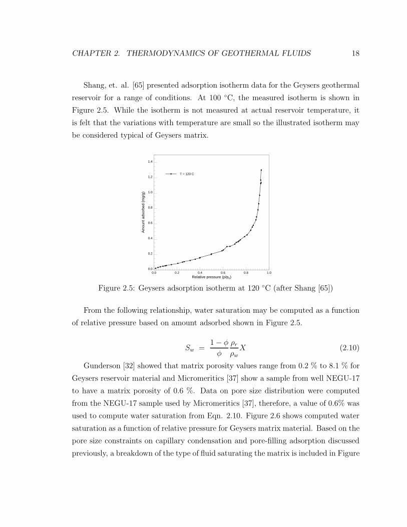
Shang, et. al. [65] presented adsorption isotherm data for the Geysers geothermal
reservoir for a range of conditions. At 100 ◦C, the measured isotherm is shown in
Figure 2.5. While the isotherm is not measured at actual reservoir temperature, it
is felt that the variations with temperature are small so the illustrated isotherm may
be considered typical of Geysers matrix.
0.0
0.2
0.4
0.6
0.8
1.0
1.2
1.4
Am
ount
ads
orbe
d (m
g/g)
0.0 0.2 0.4 0.6 0.8 1.0Relative pressure (p/po)
a a aaaa
aa
aaa
aaa
aa
aa
a aaaaaa
aa
a
aa
a
a
a
a
a
aa
a
a
a T = 120 C
Figure 2.5: Geysers adsorption isotherm at 120 ◦C (after Shang [65])
From the following relationship, water saturation may be computed as a function
of relative pressure based on amount adsorbed shown in Figure 2.5.
Sw =1− φ
φ
ρr
ρw
X (2.10)
Gunderson [32] showed that matrix porosity values range from 0.2 % to 8.1 % for
Geysers reservoir material and Micromeritics [37] show a sample from well NEGU-17
to have a matrix porosity of 0.6 %. Data on pore size distribution were computed
from the NEGU-17 sample used by Micromeritics [37], therefore, a value of 0.6% was
used to compute water saturation from Eqn. 2.10. Figure 2.6 shows computed water
saturation as a function of relative pressure for Geysers matrix material. Based on the
pore size constraints on capillary condensation and pore-filling adsorption discussed
previously, a breakdown of the type of fluid saturating the matrix is included in Figure
CHAPTER 2. THERMODYNAMICS OF GEOTHERMAL FLUIDS 19
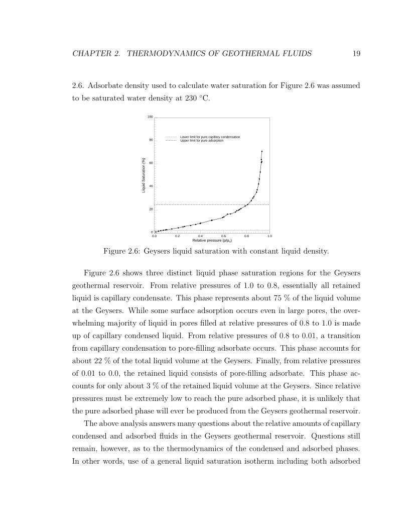
2.6. Adsorbate density used to calculate water saturation for Figure 2.6 was assumed
to be saturated water density at 230 ◦C.
0
20
40
60
80
100
Liqu
id S
atur
atio
n (%
)
0.0 0.2 0.4 0.6 0.8 1.0Relative pressure (p/po)
a a a aaaa
a aaa
aaa
aa
aa
a aaaaaa
aa
a
aa
aa
a
a
a
aaa
a
Lower limit for pure capillary condensationUpper limit for pure adsorption
Figure 2.6: Geysers liquid saturation with constant liquid density.
Figure 2.6 shows three distinct liquid phase saturation regions for the Geysers
geothermal reservoir. From relative pressures of 1.0 to 0.8, essentially all retained
liquid is capillary condensate. This phase represents about 75 % of the liquid volume
at the Geysers. While some surface adsorption occurs even in large pores, the over-
whelming majority of liquid in pores filled at relative pressures of 0.8 to 1.0 is made
up of capillary condensed liquid. From relative pressures of 0.8 to 0.01, a transition
from capillary condensation to pore-filling adsorbate occurs. This phase accounts for
about 22 % of the total liquid volume at the Geysers. Finally, from relative pressures
of 0.01 to 0.0, the retained liquid consists of pore-filling adsorbate. This phase ac-
counts for only about 3 % of the retained liquid volume at the Geysers. Since relative
pressures must be extremely low to reach the pure adsorbed phase, it is unlikely that
the pure adsorbed phase will ever be produced from the Geysers geothermal reservoir.
The above analysis answers many questions about the relative amounts of capillary
condensed and adsorbed fluids in the Geysers geothermal reservoir. Questions still
remain, however, as to the thermodynamics of the condensed and adsorbed phases.
In other words, use of a general liquid saturation isotherm including both adsorbed

CHAPTER 2. THERMODYNAMICS OF GEOTHERMAL FLUIDS 20
and condensed liquid is not possible until the properties (density, internal energy,
latent heat) of the adsorbate and condensate are understood.
2.3.2 Density of the Retained Liquid Phases
To accurately determine the pressure effects of a retained liquid phase, the density of
the retained liquid must be modeled accurately. For modeling of fluid flow in specific
geothermal reservoirs, information on the relative amounts of retained liquid must be
combined with information on liquid properties to determine the best way of modeling
retained liquid properties.
Density of the Capillary Condensed Liquid
Extrapolation of the liquid specific volume curve provides information on the density
of capillary condensed liquid. Condensed liquid phase specific volumes are shown as
a function of pressure in Figure 2.7.
0
5
10
15
20
25
Pre
ssur
e (M
Pa)
0.000 0.001 0.002 0.003 0.004 0.005Specific Volume (m^3/kg)
Bubble-Point CurveT = 100 CT = 200 CT = 300 C
Figure 2.7: Specific volume of saturated water
Due to the low compressibility of liquid water, at a given temperature, density
changes very little from liquid at saturated conditions to superheated conditions which
exist in capillary condensed liquids.
CHAPTER 2. THERMODYNAMICS OF GEOTHERMAL FLUIDS 21
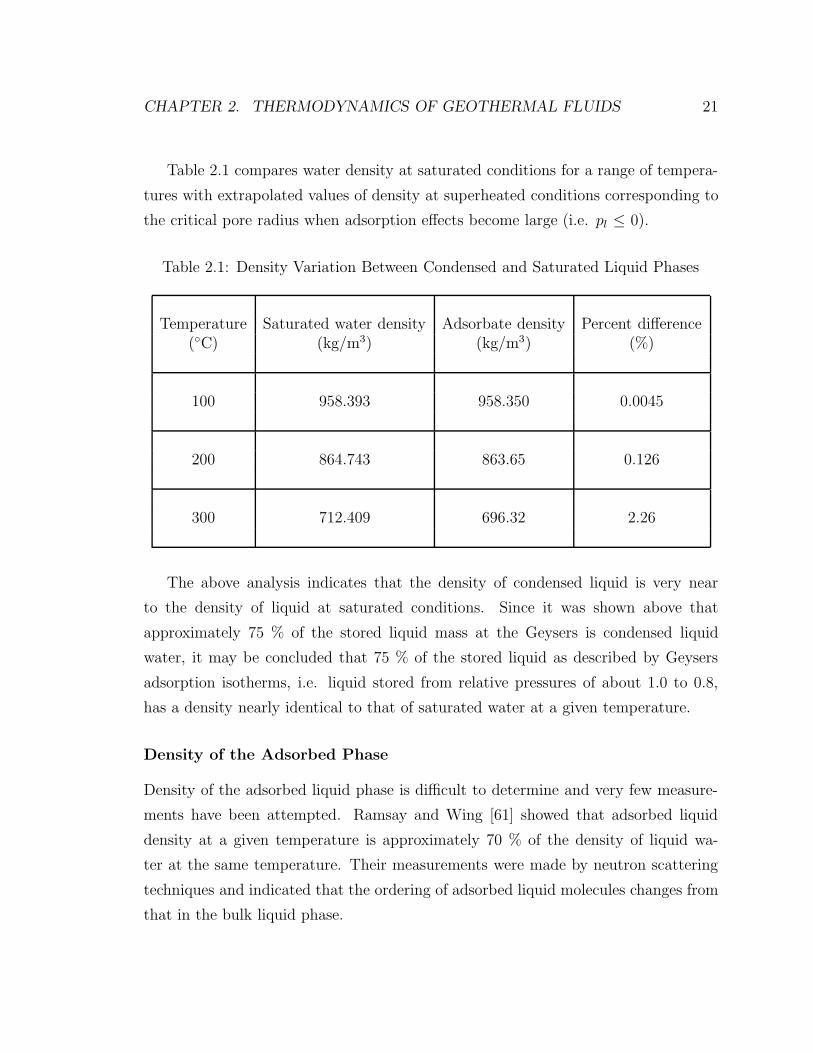
Table 2.1 compares water density at saturated conditions for a range of tempera-
tures with extrapolated values of density at superheated conditions corresponding to
the critical pore radius when adsorption effects become large (i.e. pl ≤ 0).
Table 2.1: Density Variation Between Condensed and Saturated Liquid Phases
Temperature Saturated water density Adsorbate density Percent difference(◦C) (kg/m3) (kg/m3) (%)
100 958.393 958.350 0.0045
200 864.743 863.65 0.126
300 712.409 696.32 2.26
The above analysis indicates that the density of condensed liquid is very near
to the density of liquid at saturated conditions. Since it was shown above that
approximately 75 % of the stored liquid mass at the Geysers is condensed liquid
water, it may be concluded that 75 % of the stored liquid as described by Geysers
adsorption isotherms, i.e. liquid stored from relative pressures of about 1.0 to 0.8,
has a density nearly identical to that of saturated water at a given temperature.
Density of the Adsorbed Phase
Density of the adsorbed liquid phase is difficult to determine and very few measure-
ments have been attempted. Ramsay and Wing [61] showed that adsorbed liquid
density at a given temperature is approximately 70 % of the density of liquid wa-
ter at the same temperature. Their measurements were made by neutron scattering
techniques and indicated that the ordering of adsorbed liquid molecules changes from
that in the bulk liquid phase.

CHAPTER 2. THERMODYNAMICS OF GEOTHERMAL FLUIDS 22
At the Geysers, as shown above, less than 3% of the retained liquid phase is likely
due to pore-filling adsorbed liquid. The range in relative pressures at which this phase
is dominant (0.0 to 0.01) is also quite low and it is unlikely that production of this
low density fluid will ever take place. Therefore, the liquid mass stored as low density
adsorbate can be ignored in most geothermal modeling efforts at the Geysers.
Density in the Capillary/Adsorbed Phase Transition
In the previous two sections, the density of the pure capillary condensed liquid and
the pure adsorbed phases have been established. It has also been shown that, at the
Geysers geothermal reservoir, these two phases, in essentially pure form, account for
about 78% of the stored liquid mass. The remaining liquid, accounting for 22% of
the liquid mass, is made up of both adsorbed vapor and condensed liquid. Assuming
a linear transition from condensed liquid to adsorbed liquid, it is possible to deter-
mine the density of liquid consisting of both condensate and adsorbate. Figure 2.8
shows density of the retained liquid phase as a function of pressure for the Geysers
geothermal reservoir. A similar analysis may be applied to other geothermal reser-
voirs. Effects of density assumptions for the retained liquid phase are discussed in
Chapter 4.
400
500
600
700
800
900
1000
Ret
aine
d liq
uid
dens
ity (
kg/m
3)
0.0 0.2 0.4 0.6 0.8 1.0p/po
Temp. = 200 CTemp. = 250 CTemp. = 300 C
Figure 2.8: Retained liquid density as a function of pressure (Geysers sample)

CHAPTER 2. THERMODYNAMICS OF GEOTHERMAL FLUIDS 23
Figure 2.9 shows liquid saturation inferred for the Geysers rock sample as com-
puted with Eqn. 2.10 with the varying liquid density shown in Figure 2.8. On the
same figure are water saturation values computed under the assumption of constant
water density. As may be observed, only very small differences are obtained by using
varying retained liquid densities.
0
20
40
60
80
100
Liqu
id S
atur
atio
n (%
)
0.0 0.2 0.4 0.6 0.8 1.0Relative pressure (p/po)
a a a aaaa
a aaa
aaa
aa
aa
a aaaaaa
aa
a
aa
aa
a
a
a
aaa
a
bb b
bbbb
bbb
bb
bbbb
bb
b bbbbbb
bb
b
bb
bb
b
b
b
bbb
b
a
bSaturation curve with constant adsorbate densitySaturation curve with variable adsorbate densityLower limit for pure capillary condensationUpper limit for pure adsorption
Figure 2.9: Geysers liquid saturation with variable liquid density.
2.3.3 Thermal Properties of the Retained Liquid Phases
To model heat effects of a retained liquid phase, accurate modeling of the internal
energy and the heat of vaporization/desorption of the phase is necessary. Defay and
Prigogine [19] showed that the heat of vaporization/desorption in a porous medium
may be expressed by:
hT,pv = ∆eh0 +2vl
r
[σ − T
dσ
dT
]− 2σT
r
dvl
dT+
2σvlT
r2
(∂r
∂T
)ξ
(2.11)
Eqn. 2.11 does not distinguish between capillary condensed fluid and adsorbed
fluid. Instead, it includes all heat effects generated by the phase transition of liquid
to vapor in an initially liquid filled pore. Distinguishing between thermal character-
istics of condensed and adsorbed fluids is achieved by use of pore size distribution

CHAPTER 2. THERMODYNAMICS OF GEOTHERMAL FLUIDS 24
information. The first term in Eqn. 2.11 represents the heat of evaporation of water
with no liquid curvature effects included and may be expressed as:
∆eho = RT 2∂ ln po
∂T(2.12)
The second term in Eqn. 2.11 expresses the added heat due to the extension of the
liquid surface by capillary curvature. The third term includes the heat of compression
of the water due to capillary condensation. The fourth term expresses the the added
heat due to an increase in the solid surface area as the pore is emptied. The fourth
term is not straightforward to evaluate since it depends on the pore distribution in
the solid matrix and the corresponding amount of adsorbed liquid associated with
that range of pore sizes. The pore-dependent term is defined as:
(∂r
∂T
)ξ
=dr
dVl
· ∂vl
∂T· nl (2.13)
where, dr/dVl is obtained from pore size measurements and, nl is a measure of the
amount adsorbed or condensed.
In this research, a pore size distribution measured from a Geysers rock sample was
used as a basis for determining the effects of pore drying on the heat of vaporization.
Nitrogen adsorption was used for determining pore size distributions and adsorbed
mass in. All measurements were carried out by Micromeritics [37] on a sample taken
from well NEGU-17 at the Geysers. In the sample studied, porosity was determined
to be 0.6 % which is consistent with matrix porosity reported by Gunderson [32].
Pore volume as a function of pore radius is shown in Figure 2.3. The rate of change
of radius with respect to pore volume as a function of radius (needed in Eqn. 2.11) is
shown in Figure 2.10. Worth noting from Figure 2.3 is the fact that pores of radius
less than 50 A contribute very little to the total pore volume.
Figure 2.11 shows the magnitude of heat effects due to the extension of the liquid
interface as surface curvature occurs. As liquid is evaporated from a curved interface,
more energy is required than in evaporation of an uncurved interface due to an in-
creased stretching of the curved interface. As is shown in Figure 2.11, heat effects due

CHAPTER 2. THERMODYNAMICS OF GEOTHERMAL FLUIDS 25
to surface stretching are quite small. The maximum addition to the heat of vapor-
ization due to surface stretching is about 2 %. Heat effects due to surface stretching
are assumed to terminate when pore filling adsorption dominates (re ≈ 35 A) since
adsorbate is assumed to exist as a separate phase.
0.00
0.05
0.10
0.15
0.20
0.25dr
/dV
l (m
kg/
m3)
101 102 103
Pore Size (Angstrom)
Figure 2.10: Rate of change of radius with respect of volume (Geysers sample)

CHAPTER 2. THERMODYNAMICS OF GEOTHERMAL FLUIDS 26
0
1
2
3
4
5
Per
cent
age
of F
lat-
Sur
face
Hea
t of V
apor
izat
ion
(%)
102 103 104
Pore Radius (Angstrom)
100 C200 C300 C
Figure 2.11: Surface extension effects on the heat of vaporization

CHAPTER 2. THERMODYNAMICS OF GEOTHERMAL FLUIDS 27
0
1
2
3
4
5
Per
cent
age
of F
lat-
Sur
face
Hea
t of V
apor
izat
ion
(%)
102 103 104
Pore Radius (Angstrom)
100 C200 C300 C
Figure 2.12: Liquid compression effects on the heat of vaporization
Figure 2.12 shows the magnitude of heat effects due to the capillary compres-
sion of condensed liquid. Figure 2.12 shows that more heat is required to evaporate
capillary condensed liquid than flat-surface condensed liquid since attractive forces
between fluid particles have been increased. The increase in evaporation energy is
shown, however, to be small. The maximum effects of capillary compression on heat
of vaporization are shown to be a 0.5 % increase. Heat effects due to capillary com-
pression are assumed to terminate when pore filling adsorption dominates (re ≈ 35 A)
since adsorbate is assumed to exist as a separate phase with no capillary compression
effects.
Figure 2.13 shows the magnitude of heat effects due to an increase in the solid
surface area as the pore is emptied. In other words, this figure shows the added
energy needed to dry a pore as liquid recedes. Figure 2.13 shows that more heat is
required to evaporate liquid retained in pores since liquid/solid attractive forces must
be overcome. The magnitude of this term will vary with material tested but it is
shown to be large for Geysers core material in very small pores. Heat effects due to
pore drying influence the heat of vaporization for the entire range of pore sizes and,
therefore, include the effects of both evaporation and desorption. The curves shown
in Figure 2.13 are not smooth due to data used in calculating the curves. The rate

CHAPTER 2. THERMODYNAMICS OF GEOTHERMAL FLUIDS 28
0
20
40
60
80
100
Per
cent
age
of F
lat-
Sur
face
Hea
t of V
apor
izat
ion
(%)
101 102 103 104
Pore Radius (Angstrom)
100 C200 C300 C
Figure 2.13: Pore drying effects on the heat of vaporization
of change of radius with respect to pore volume, shown in Figure 2.10, was used to
compute pore drying effects and the roughness in the curve translated to roughness
in the heat of pore drying curve shown in Figure 2.13.
Figure 2.14 shows the heat of vaporization for water as a function of pore radius
for a range of temperatures. A notation is included in the figure to denote the 100 A
pore radius. About 90 % of Geysers liquid resides in pores of radius larger than 100
%. It is clear from Figure 2.14 that most of the liquid in the Geysers reservoir may be
considered saturated liquid from a heat balance standpoint. For very small pores, the
heat of vaporization effects can become large, but for a large range of pore sizes, heat
of vaporization effects are not significant. Comparison of heat of vaporization effects
with pore size distribution data at the Geysers shows that the heat of vaporization
for about 80 % of the liquid stored varies from flat surface values by only about 3
%. Further, less than 1 % of the stored liquid has heat of vaporization values varying
from flat surface values by more than 15 %. These results lead to the conclusion
that, for most of the liquid stored at the Geysers, heat of vaporization does not vary
significantly from saturated liquid values at a given temperature. Therefore, it is
reasonable to use heat of vaporization values based on flat surface thermodynamics.

CHAPTER 2. THERMODYNAMICS OF GEOTHERMAL FLUIDS 29
2000000
2200000
2400000
2600000
2800000
3000000
3200000
3400000
3600000
3800000
4000000
Hea
t of V
apor
izat
ion
(J/k
g)
10-9 10-8 10-7 10-6
Pore Radius (Angstrom)
aaaaa
bbbbbccccc
a
b
c
100 C (Porous medium values)200 C (Porous medium values)300 C (Porous medium values)Radius representing 90% of adsorbed mass at Geysers100 C (Flat surface values)200 C (Flat surface values)300 C (Flat surface values)
Figure 2.14: Effects of pore size and temperature on the heat of vaporization
Finally, Eqn. 2.11 shows that the increase in heat of vaporization is a surface phe-
nomenon. In other words, the properties of the bulk retained liquid do not change
significantly as liquid condenses, only the surface forces change. This observation,
combined with the result that the vast majority of the liquid stored at the Geysers
has thermal properties within a few percent of saturated water leads us to the con-
clusion that it may be assumed that the internal energy of the retained liquid phase
is the same as the internal energy of the bulk liquid phase. So, from a heat balance
standpoint, adsorbed and capillary condensed liquid may be considered identical to
liquid water at saturated conditions.
2.3.4 Summary of Thermodynamic Properties
Analysis of the thermodynamics of retained liquids in geothermal reservoirs indicates
that the properties may vary significantly from the properties of saturated liquid. It
is shown that for pore sizes present in geothermal reservoirs, both density and heat
of vaporization may be significantly altered.
Density of the capillary condensed phase varies from saturated density in large
pores (re ≈ 104A at 300 ◦C) to slightly less than saturated density in extremely small
pores (re ≈ 50 A at 300 ◦C). Table 2.1 shows that the maximum density difference

CHAPTER 2. THERMODYNAMICS OF GEOTHERMAL FLUIDS 30
is 2.26%. Even without any knowledge of the pore size distribution in a geothermal
reservoir, density differences for the capillary condensed liquid were shown to be
negligible.
Pore-filling adsorbate density was shown to be significantly less than saturated
liquid density at a given temperature but, for the Geysers reservoir, was shown to
account for a very small fraction of the total mass. Based on a simple linear relation,
a relationship between retained liquid density and relative pressure was derived for
the Geysers geothermal reservoir.
Heat of vaporization of the adsorbed phase varies from the heat of vaporization of
liquid water in large pores (re ≥ 104A) to a maximum of about 1.5 times that value
in the smallest pores that may be occupied by a water molecule (re ≈ 2A). Internal
energy effects were shown to be small since heat of vaporization effects are shown
to be surface, rather than bulk liquid, dependent (Eqn. 2.11). Also, since internal
energy of the vapor phase is shown to be virtually identical to the internal energy of
vapor in the absence of a porous medium and heat of vaporization effects are shown
to be small in the Geysers geothermal reservoir, it is inferred that the internal energy
of the liquid phase must also be similar to the internal energy of a liquid phase in the
absence of a porous medium.
Thus, thermal properties of retained liquid at the Geysers were shown to be nearly
identical to the properties of liquid water at saturated conditions.

Chapter 3
Analysis of the Energy Balance
In computing the heat balance in geothermal reservoirs, a number of assumptions are
commonly made. First, the assumption of thermal equilibrium is made whether an
adsorbed phase is present or not. No calculations have been presented to determine
if this is a good assumption for a range of conditions. Second, assumptions about
the sizes of various terms in the energy balance on flow through porous media are
often made without justification. A systematic analysis of the sizes of terms in the
energy balance is needed to determine which terms may be neglected under a range
of conditions. Third, the influence of an adsorbed phase on the fate of injected water
must be studied to determine if the presence of an adsorbed phase significantly effects
the rate of boiling of injected water.
The assumption of thermal equilibrium was tested, the relative importance of each
term in the overall energy balance was determined, and the fate of injected water was
studied for a range of conditions.
3.1 Validity of Thermal Equilibrium Assumption
In most studies of flow in geothermal reservoirs, the assumption of instantaneous
thermal equilibrium is made. In other words, the time for the diffusion of heat
from the matrix to the liquid is assumed to be much less than the residence time
of the fluid. To test the validity of this common assumption, a comparison of fluid
31

CHAPTER 3. ANALYSIS OF THE ENERGY BALANCE 32
velocity with heat diffusion velocity was carried out for a range of reservoir conditions.
Computations were made for the flow of single phase liquid and for the flow of liquid
in the presence of an adsorbed phase.
Single-phase fluid flow may be modeled by Darcy’s law:
v =k
µ
dp
dx(3.1)
Since most geothermal reservoirs are characterized by fracture porosity, pores may
be approximated by a slit. For simplicity, heat conduction in a slit was modeled by
heat conduction across a space spanned by two parallel planes as given by Carslaw
and Jaeger [15]:
T (y, z) =4To
π
∞∑n=0
(1
2n + 1
)exp
(−κ(2n + 1)2π2t/l2
)sin
[(2n + 1)πy
l
](3.2)
where; To is the initial temperature, and l is the separation between the parallel planes
(i.e. the fracture width), y is the distance measured from one of the planes, and κ,
the thermal diffusivity, is defined as the ratio of thermal conductivity, kt, and the
heat capacity per unit volume, ρCp.
κ =kt
ρCp(3.3)
To compare fluid residence time to characteristic heat diffusion time, reservoir
rock and fluid characteristics must be assumed. Data for this analysis was taken from
the range of properties at the Geysers geothermal field. From pressure data at the
Geysers collected by Barker et. al. [7], a maximum pressure gradient of about 450
Pa/m was obtained. At 230 ◦C, fluid viscosity is 0.116×10⁻³ Pa·s and permeability
can range from about 1×10⁻¹² m2 in large pores and fractures to about 1×10⁻¹⁶
m2 in the matrix. Based on these ranges of values, a range in fluid velocity may be
calculated and used to determine fluid residence time before the onset of boiling. The
range of liquid velocity was computed from 4×10⁻⁶ m/s in large pores and fractures
to 4×10⁻¹⁰ m/s in the reservoir matrix.
CHAPTER 3. ANALYSIS OF THE ENERGY BALANCE 33
When cool injectate is heated by contact with hot rock, the thermal diffusivity
of the liquid changes. Computation of the thermal diffusivity of water over a range
of temperatures was carried out to determine the magnitude of this variation and
to determine if one value of thermal diffusivity could be used in thermal diffusion
computations. Table 3.1 shows the tabulated values of the thermal diffusivity of
water. The thermal diffusivity is shown to reach a maximum at about 150 ◦C and
it may also be observed that the diffusivity does not vary much for a wide range
of temperatures. In fact, diffusivity values do not vary by more than 11% from the
diffusivity value calculated at 50 ◦C. Therefore, the thermal diffusivity of liquid water
at 50 ◦C, (1.563×10⁻⁷) was used in thermal calculations.
A dimensionless temperature was defined as:
T =T
To
(3.4)
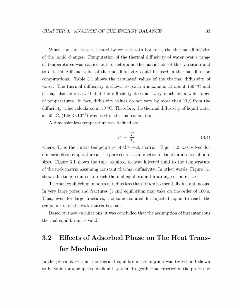
where, To is the initial temperature of the rock matrix. Eqn. 3.2 was solved for
dimensionless temperature at the pore center as a function of time for a series of pore
sizes. Figure 3.1 shows the time required to heat injected fluid to the temperature
of the rock matrix assuming constant thermal diffusivity. In other words, Figure 3.1
shows the time required to reach thermal equilibrium for a range of pore sizes.
Thermal equilibrium in pores of radius less than 10 µm is essentially instantaneous.
In very large pores and fractures (1 cm) equilbrium may take on the order of 100 s.
Thus, even for large fractures, the time required for injected liquid to reach the
temperature of the rock matrix is small.
Based on these calculations, it was concluded that the assumption of instantaneous
thermal equilibrium is valid.
3.2 Effects of Adsorbed Phase on The Heat Trans-
fer Mechanism
In the previous section, the thermal equilibrium assumption was tested and shown
to be valid for a simple solid/liquid system. In geothermal reservoirs, the process of

CHAPTER 3. ANALYSIS OF THE ENERGY BALANCE 34
0.0
0.2
0.4
0.6
0.8
1.0
Dim
ensi
onle
ss T
empe
ratu
re a
t Por
e C
ente
r
10-4 10-3 10-2 10-1 1 10 102
Time (s)
r = 1.0 µmr = 10.0 µmr = 100.0 µmr = 1.0 mmr = 1.0 cm
Figure 3.1: Time required for thermal equilibration of injected fluid
boiling injected liquid is a complicated process which may be affected by the presence
of an adsorbed phase. In this section, the influence of the adsorbed phase on the heat
transfer mechanism was studied and conclusions were drawn about the effects of an
adsorbed phase on the boiling of injected fluids.
An expression for the heat transfer coefficient in a porous material was derived by
Navruzov [51]:
h =kf
δf
(3.5)
where, kf is the thermal conductivity of the liquid in the pore and δf is the thin liquid
layer near the solid surface over which most of the thermal resistance is concentrated.
In porous systems with no adsorbed phase present, the thermal conductivity is that of
water at a given temperature and pressure. When an adsorbed phase is present, heat
transfer will be altered by a thin film of adsorbed water at a temperature different
than that of injected water. Table 3.1 presents the thermal conductivity of saturated
water for a range of temperatures. The maximum variation in thermal conductivity
over a range of temperatures likely in geothermal reservoirs is always less that 15

CHAPTER 3. ANALYSIS OF THE ENERGY BALANCE 35
%. Therefore, assuming that the thickness is constant over which heating resistance
occurs, the maximum variation in heat transfer is also 15 %. When an adsorbed
phase is present, the temperature and, therefore, the thermal conductivity of the
adsorbed phase must be larger than the thermal conductivity of the injected water.
This means that the effect of an adsorbed phase on the heat transfer to injected
water is an increase in the transfer rate resulting in more rapid boiling than without
adsorption, thus enhancing the validity of the thermal equilibrium assumption. This
increase in heat transfer is small, however, limited to a 15 % increase over the transfer
rate without an adsorbed phase present.
3.3 The Energy Balance
A detailed analysis of the energy balance is necessary to determine the effects of an
adsorbed phase on the storage and transfer of energy in geothermal reservoirs. The
purpose of this section is to study the heat balance to determine the size of each term
and the range of conditions for which each term is important. Information on the
importance of each term may then be used in modeling the flow of geothermal fluids.
Garg and Pritchett [27] performed an analysis of an energy balance for geothermal
reservoirs in the absence of an adsorbed phase. Their work was used as a basis from
which to study the heat balance with an adsorbed phase present.
In deriving the energy balance it was assumed that the rock matrix is incompress-
ible (i.e. porosity is constant). The incompressible matrix assumption is a good one
in most geothermal reservoirs which are usually characterized by very small fracture
porosity. It was also assumed that the fluids and the rock matrix are in local thermal
equilibrium. The assumptions of local thermal equilibrium was shown to be valid
earlier in this chapter where it was proven that equilibrium between the rock matrix
and the flowing fluids occurs rapidly in low porosity systems. The complete energy
balance for flow in a geothermal reservoir is:
∂
∂t[(1− φ)ρrEr + φSwρwEw + φSvρvEv + φSaρaEa]
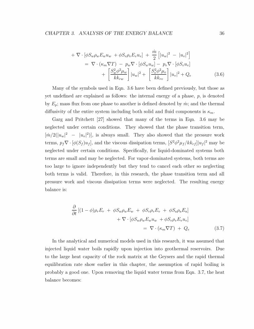
CHAPTER 3. ANALYSIS OF THE ENERGY BALANCE 36
+ ∇ · [φSwρwEwuw + φSvρvEvuv] +m
2
[|uw|2 − |uv|2
]= ∇ · (κm∇T ) − pw∇ · [φSwuw]− pv∇ · [φSvuv]
+
[S2
wφ2µw
kkrw
]|uw|2 +
[S2
vφ2µv
kkrv
]|uv|2 + Qe (3.6)
Many of the symbols used in Eqn. 3.6 have been defined previously, but those as
yet undefined are explained as follows: the internal energy of a phase, p, is denoted
by Ep; mass flux from one phase to another is defined denoted by m; and the thermal
diffusivity of the entire system including both solid and fluid components is κm.
Garg and Pritchett [27] showed that many of the terms in Eqn. 3.6 may be
neglected under certain conditions. They showed that the phase transition term,
[m/2(|uw|2 − |uv|2)], is always small. They also showed that the pressure work
terms, pf∇ · [φ(Sf)uf ], and the viscous dissipation terms, [S2φ2µf/kkrf ]|uf |2 may be
neglected under certain conditions. Specifically, for liquid-dominated systems both
terms are small and may be neglected. For vapor-dominated systems, both terms are
too large to ignore independently but they tend to cancel each other so neglecting
both terms is valid. Therefore, in this research, the phase transition term and all
pressure work and viscous dissipation terms were neglected. The resulting energy
balance is:
∂
∂t[(1− φ)ρrEr + φSwρwEw + φSvρvEv + φSaρaEa]
+ ∇ · [φSwρwEwuw + φSvρvEvuv]
= ∇ · (κm∇T ) + Qe (3.7)
In the analytical and numerical models used in this research, it was assumed that
injected liquid water boils rapidly upon injection into geothermal reservoirs. Due
to the large heat capacity of the rock matrix at the Geysers and the rapid thermal
equilibration rate show earlier in this chapter, the assumption of rapid boiling is
probably a good one. Upon removing the liquid water terms from Eqn. 3.7, the heat
balance becomes:
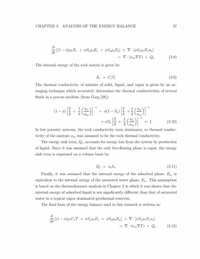
CHAPTER 3. ANALYSIS OF THE ENERGY BALANCE 37
∂
∂t[(1− φ)ρrEr + φSvρvEv + φSaρaEa] + ∇ · [φSvρvEvuv]
= ∇ · (κm∇T ) + Qe (3.8)
The internal energy of the rock matrix is given by:
Er = CrTr (3.9)
The thermal conductivity of mixture of solid, liquid, and vapor is given by an av-
eraging technique which accurately determines the thermal conductivities of several
fluids in a porous medium (from Garg [28]):
(1− φ)[2
3+
1
3
(κr
κm
)]−1
+ φ(1− Sv)[2
3+
1
3
(κa
κm
)]−1
+ φSv
[2
3+
1
3
(κv
κm
)]−1
= 1 (3.10)
In low porosity systems, the rock conductivity term dominates, so thermal conduc-
tivity of the mixture κm was assumed to be the rock thermal conductivity.
The energy sink term, Qe, accounts for energy lost from the system by production
of liquid. Since it was assumed that the only free-flowing phase is vapor, the energy
sink term is expressed on a volume basis by:
Qe = uvhv (3.11)
Finally, it was assumed that the internal energy of the adsorbed phase, Ea, is
equivalent to the internal energy of the saturated water phase, Ew. This assumption
is based on the thermodynamic analysis in Chapter 2 in which it was shown that the
internal energy of adsorbed liquid is not significantly different than that of saturated
water in a typical vapor dominated geothermal reservoir.
The final form of the energy balance used in this research is written as:
∂
∂t[(1− φ)ρrCrT + φSvρvEv + φSaρaEw] + ∇ · [φSvρvEvuv]
= ∇ · (κm∇T ) + Qe (3.12)

CHAPTER 3. ANALYSIS OF THE ENERGY BALANCE 38
Table 3.1: Thermal Diffusivity of Water
Temp Cp ρ K κ(◦C) (J/kg·K) (kg/m3) (W/m·K) (m2/s)
20.0 4170.9 1000.0 0.60023 1.439×10⁻⁷
50.0 4172.7 989.73 0.64537 1.563×10⁻⁷
70.0 4170.9 979.50 0.66503 1.635×10⁻⁷
100.0 4170.9 960.22 0.68125 1.686×10⁻⁷
120.0 4239.0 945.05 0.68547 1.711×10⁻⁷
150.0 4170.9 919.05 0.68446 1.732×10⁻⁷
200.0 4170.9 866.60 0.66553 1.716×10⁻⁷
250.0 4170.9 799.10 0.62140 1.601×10⁻⁷

Chapter 4
Semi-Analytical Model
In analyzing the effects of adsorption on flow through porous media, it is important
to isolate, as clearly as possible, the effects of adsorption so the physics of adsorption-
influenced flow may be fully understood. Derivation of the conservation equation for
fluid flow with adsorption leads to a highly nonlinear equation which may be solved
either numerically or by analytical methods. While there are benefits to solving the
equation in either way, an analytical solution is preferred because adsorption effects
are more clearly isolated and the effects of adsorption may be studied without the
use of costly and complicated numerical simulation.
In this case, due to the highly nonlinear nature of the equation to be solved, a
purely analytical solution was found to be impossible without oversimplification of the
problem. Therefore, a semi-analytical procedure was used which couples the method
of similarity analysis with finite difference solution of an ordinary differential equation.
Similarity analysis was used because it allows the partial differential equation for
vapor flow with adsorption to be solved in a general manner and allows for separation
of adsorption effects.
4.1 Derivation of Analytical Solution
The conservation of mass for isothermal vapor flow with an adsorption phase present
is expressed as:
39
CHAPTER 4. SEMI-ANALYTICAL MODEL 40
φ∂ρv(1− Sa)
∂t+ φρa
∂Sa
∂t+ ∇ · (uvρv) = 0 (4.1)
The first two terms in the above equation describe the time rate of change of vapor
and adsorbate mass, respectively. Since adsorbate does not flow freely, the third term
involves only free vapor. Rearranging Eqn. 4.1 and imposing the restriction of one
dimensional flow:
φ∂(ρv − ρvSa)
∂t+ φρa
∂Sa
∂t+
∂
∂x(uvρv) = 0 (4.2)
The adsorbate saturation, Sa is pressure dependent and is described by an ad-
sorption isotherm, X(p):
Sa =1− φ
φ
ρr
ρaX(p) (4.3)
Upon substitution of Eqn. 4.3 into Eqn. 4.2 and simplifying:
[1−
(1− φ
φ
)ρr
ρa
X
]∂ρv
∂t+
[(1− φ
φ
)ρr
ρa
(ρa − ρv)
]∂X
∂t+
1
φ
∂
∂x(uvρv) = 0 (4.4)
Eqn. 4.4 may be simplified further by observing:
∂X
∂t=
∂ρv
∂t
∂X
∂ρv
(4.5)
Substitution of Eqn. 4.5 into Eqn. 4.4 yields:
[{1−
(1− φ
φ
)ρr
ρaX} + {∂X
∂ρv
(1− φ
φ
)ρr
ρa(ρa − ρv)}
]∂ρv
∂t+
1
φ
∂
∂x(uvρv) = 0
(4.6)
Vapor velocity is obtained from Darcy’s law:
uv = − k
µv
∂p
∂x(4.7)
Upon substitution of Eqn. 4.7 into Eqn. 4.6:

CHAPTER 4. SEMI-ANALYTICAL MODEL 41
φA(p)∂ρv
∂t=
∂
∂x
(kρv
µv
∂p
∂x
)= 0 (4.8)
where the nonlinear adsorption term, A(p), is given by:
A(p) = {1−(
1− φ
φ
)ρr
ρa
X} + {∂X
∂ρv
((1− φ
φ
)ρr −
(1− φ
φ
)ρrρv
ρa
)} (4.9)
Pressure and density of the vapor are related by the real gas law:
pV = znRvT (4.10)
ρv =Mp
zRvT(4.11)
The continuity equation, Eqn. 4.8, may be written in terms of pressure by using
the real gas law. Substituting the expression for vapor density, Eqn. 4.11 into Eqn.
4.8, the continuity equation becomes:
∂
∂x
[1
µz
∂p2
∂x
]=
φA(p)cv
kz
∂p2
∂t(4.12)
It is important to understand the form of the compressibility term, cv. First,
since vapor compressibility is much larger that rock compressibility, the total system
compressibility in a vapor dominated system is approximated by the vapor compress-
ibility. Second, the form of the vapor compressibility is determined by analysis over
a range of temperature and pressure. The expression for vapor compressibility is:
cv =−1
V
(∂V
∂p
)T
=1
ρv
(∂ρv
∂p
)T
(4.13)
Combining Eqns. 4.13 and 4.11 leads to the following general expression for
compressibility:
cv =1
p− 1
z
dz
dp(4.14)
For the range of pressure encountered in geothermal reservoirs, compressibility may
be closely approximated by:

CHAPTER 4. SEMI-ANALYTICAL MODEL 42
cv =1
p(4.15)
Figures 4.1 and 4.2 compare NIST [26] tabulated steam viscosity and viscosity
approximated by 1/p for a range of pressures at 200 and 300 ◦C, respectively. The
figures confirm the assumption that for the temperatures and pressures found in most
geothermal reservoirs, compressibility may be approximated by 1/p. This approxi-
mation may be used in Eqn. 4.12.
0
2
4
6
8
10
12
Com
pres
sibi
lity
(1/M
Pa)
0.0 0.2 0.4 0.6 0.8 1.0 1.2 1.4 1.6 1.8 2.0Pressure (MPa)
Compressibility of Steam at 200 C
NIST values1/p
Figure 4.1: Compressibility of steam at 200 C
Eqn. 4.12 is quite nonlinear in its current form. Viscosity (µ), compressibility
(c), the adsorptive nonlinear term (A(p)), and the gas deviation factor (z) are all
functions of pressure. To eliminate some of the nonlinearities and to simplify the
expression somewhat, the real gas pseudopressure derived by Al-Hussainy, Ramey,
and Crawford [3] was introduced:
m(p) =∫ p
pb
2p
µzdp (4.16)
Use of Eqn. 4.16 in Eqn. 4.12 leads to the continuity equation in terms of pseudo-
pressure:

CHAPTER 4. SEMI-ANALYTICAL MODEL 43
0
2
4
6
8
10
12
Com
pres
sibi
lity
(1/M
Pa)
0 1 2 3 4 5Pressure (MPa)
Compressibility of Steam at 300 C
NIST values1/p
Figure 4.2: Compressibility of steam at 300 C
∂2m(p)
∂x2=
φA(p)cvµ
k
∂m(p)
∂t(4.17)
Eqn. 4.17 is still highly nonlinear. By introduction of Agarwal pseudotime [2],
the remaining pressure dependent terms (except for the adsorptive nonlinear term)
are eliminated. The Agarwal pseudotime [2] has been altered to include the constant
porosity and permeability terms.
ta(p) =∫ p
pb
k[
dtdp
]φµct
dp (4.18)
Substitution of Eqn. 4.18 into 4.17 leads to:
∂2m(p)
∂x2= A(p)
∂m(p)
∂ta(p)(4.19)
Now, the only nonlinear effects are those due to adsorptive effects and are completely
isolated in the nonlinear term, A(p).
For a semi-infinite linear reservoir producing at a constant pressure well, the
boundary conditions for Eqn. 4.19 may be written:

CHAPTER 4. SEMI-ANALYTICAL MODEL 44
Inner Boundary : m(p)(x = 0, t) = m(pw) (4.20)
Outer Boundary : m(p)(x →∞, t) = m(pi) (4.21)
Initial Condition: m(p)(x, t = 0) = m(pi) (4.22)
4.1.1 Analysis of Adsorption Pressure Effects.
By studying the relative sizes of components of the nonlinear term, A(p) given in
Eqn. 4.9, it is possible to determine the importance of various adsorption effects.
The nonlinear adsorptive term is influenced by both the amount of fluid adsorbed
(the second term on the right in Eqn. 4.9) and by the rate at which this fluid either
adsorbs or desorbs (the third term on the right in Eqn. 4.9).
A range of adsorption isotherms were used to compute A(p) over a range of reser-
voir temperatures. Langmuir isotherms with widely varying shapes and magnitudes
were used to determine adsorption effects. An analysis follows on the relative sizes of
the terms in the adsorptive nonlinear function, A(p).
Adsorption Isotherms
A Langmuir model was chosen to represent adsorption isotherms. This model was
used because a large range of isotherm shapes are easily modeled. Langmuir isotherms
usually described by the following relationship:
X(p/ps) =p/ps
a + bp/ps(4.23)
Correa and Ramey [16] showed that the Langmuir equation, Eqn. 4.23 can be rewrit-
ten in a different form:
X(p/ps) = d
[cp/ps
1 + (c− 1)p/ps
](4.24)
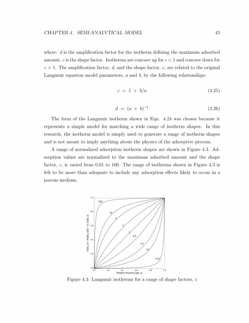
CHAPTER 4. SEMI-ANALYTICAL MODEL 45
where: d is the amplification factor for the isotherm defining the maximum adsorbed
amount, c is the shape factor. Isotherms are concave up for c < 1 and concave down for
c > 1. The amplification factor, d, and the shape factor, c, are related to the original
Langmuir equation model parameters, a and b, by the following relationships:
c = 1 + b/a (4.25)
d = (a + b)−1 (4.26)
The form of the Langmuir isotherm shown in Eqn. 4.24 was chosen because it
represents a simple model for matching a wide range of isotherm shapes. In this
research, the isotherm model is simply used to generate a range of isotherm shapes
and is not meant to imply anything about the physics of the adsorptive process.
A range of normalized adsorption isotherm shapes are shown in Figure 4.3. Ad-
sorption values are normalized to the maximum adsorbed amount and the shape
factor, c, is varied from 0.01 to 100. The range of isotherms shown in Figure 4.3 is
felt to be more than adequate to include any adsorption effects likely to occur in a
porous medium.
0.0
0.2
0.4
0.6
0.8
1.0
X(p
/p_s
) =
dc(
p/p_
s)/[1
+ (
c-1)
p/p_
s]
0.0 0.2 0.4 0.6 0.8 1.0Relative Pressure (p/p_s)
0.01
0.1
0.2
0.5
1
2
5
10
100
Figure 4.3: Langmuir isotherms for a range of shape factors, c
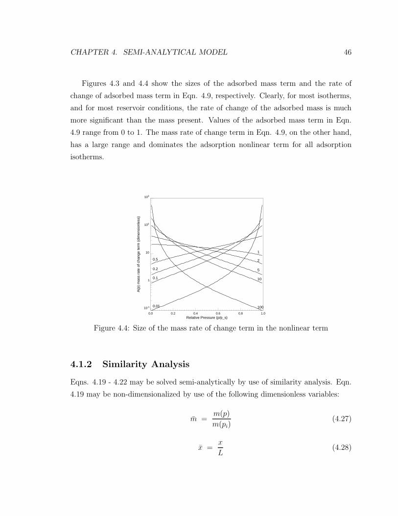
CHAPTER 4. SEMI-ANALYTICAL MODEL 46
Figures 4.3 and 4.4 show the sizes of the adsorbed mass term and the rate of
change of adsorbed mass term in Eqn. 4.9, respectively. Clearly, for most isotherms,
and for most reservoir conditions, the rate of change of the adsorbed mass is much
more significant than the mass present. Values of the adsorbed mass term in Eqn.
4.9 range from 0 to 1. The mass rate of change term in Eqn. 4.9, on the other hand,
has a large range and dominates the adsorption nonlinear term for all adsorption
isotherms.
10-1
1
10
102
103
A(p
) m
ass
rate
of c
hang
e te
rm (
dim
ensi
onle
ss)
0.0 0.2 0.4 0.6 0.8 1.0Relative Pressure (p/p_s)
100
10
5
2
1
0.5
0.2
0.1
0.01
Figure 4.4: Size of the mass rate of change term in the nonlinear term
4.1.2 Similarity Analysis
Eqns. 4.19 - 4.22 may be solved semi-analytically by use of similarity analysis. Eqn.
4.19 may be non-dimensionalized by use of the following dimensionless variables:
m =m(p)
m(pi)(4.27)
x =x
L(4.28)

CHAPTER 4. SEMI-ANALYTICAL MODEL 47
t =t(p)
L2(4.29)
Upon substitution of Eqns. 4.27 - 4.29 into Eqn. 4.19 a dimensionless equation is
obtained:
∂2m
∂x2= A(m)
∂m
∂t(4.30)
with dimensionless boundary conditions:
Inner Boundary : m(x = 0, t) =m(pw)
m(pi)= mo (4.31)
Outer Boundary : m(x →∞, t) = 1 (4.32)
Initial Condition: m(x, t = 0) = 1 (4.33)
The partial differential equation, Eqn. 4.30, may be converted to an ordinary
differential equation by assuming the the dimensionless pseudopressure may be ex-
pressed as:
m = Θ(t)f(η) (4.34)
where η is the similarity expression:
η =x
2√
t(4.35)
The constant inner boundary condition (Eqn. 4.20) specifies the value of Θ(t):
Θ(t) = mo (4.36)
Upon substitution of Eqns. 4.34 - 4.36 into Eqn. 4.30 an ordinary differential
equation is obtained:
d2f
dη2+ 2ηA(f)
df
dη= 0 (4.37)

CHAPTER 4. SEMI-ANALYTICAL MODEL 48
with boundary conditions:
Inner Boundary : f(η → 0) = 1 (4.38)
Outer Boundary : f(η →∞) =1
mo
(4.39)
Eqn. 4.37 must be solved by numerical methods for two reasons. First, the
boundary conditions represent values of f(η) at two different boundaries so numerical
methods must be employed to determine the shape of the function between endpoints.
Second, the nonlinear term, A(f) is not solved analytically, but, rather, is solved by
means of table lookup so a numerical scheme is necessary to introduce accurate values
of A(f). A finite difference solution was chosen for this purpose since the solution, f,
is a simple function of η.
In discretized form Eqn. 4.37 becomes:
[fi+1 − 2fi + fi−1
h2
]+ ηA(f)
[fi+1 − fi−1
h
]= 0 (4.40)
where, h represents a discrete step in η. Eqn. 4.40 may be written in matrix form
and solved numerically:
β1 α1
γ1 β2 α2
γ3 β3 α3
· · ·· · ·
γN−2 βN−2 αN−2
γN−1 βN−1
f1
f2
f3
··
fN−2
fN−1
=
−γ1f0
0
0
··0
−αN−1fN−1
(4.41)
Entries in the matrix are:
αi =
[1
h2+
ηA(f)
h
](4.42)

CHAPTER 4. SEMI-ANALYTICAL MODEL 49
βi =[− 2
h2
](4.43)
γi =
[1
h2− ηA(f)
h
](4.44)
Solution of Eqn. 4.41 for several adsorption isotherm shapes yields a range of
curves for f(η) vs. η as a function of the shape factor describing the adsorbed phase.
The computed similarity functions are shown in Figure 4.5. The shape factors used
correspond to those shown in Figure 4.3.
0
2000
4000
6000
8000
10000
f(η)
0.0 0.5 1.0 1.5 2.0 2.5η
a
a
a
a
a
a
a
aa
a a a a a
a No adsorbed phased = 0.0010, c = 0.01d = 0.0010, c = 0.10d = 0.0010, c = 0.20d = 0.0010, c = 0.50d = 0.0010, c = 1.00d = 0.0010, c = 2.00d = 0.0010, c = 5.00d = 0.0010, c = 10.0d = 0.0010, c = 100.
Figure 4.5: Similarity function for a range of adsorption isotherms
4.1.3 Solution Procedure
The matrix problem that was solved is shown in Eqns. 4.41 through 4.44. The
tridiagonal matrix problem was solved by use of the Thomas algorithm. Since the
problem is nonlinear, an iterative procedure was used.
1. Initial guesses of f(η) vs. η are made. The lower boundary of f(η) = 1 is
fixed at η = 0. The upper boundary of f(η) = 1/m0 is fixed at an arbitrary η

CHAPTER 4. SEMI-ANALYTICAL MODEL 50
sufficiently large that errors are not introduced (selection of the upper boundary
of η is discussed more fully later in this section).
2. The initial guesses for f(η) are distributed in a linear fashion between the fixed
endpoints. The initial guesses for the f(η) are saved as old values.
3. The nonlinear adsorption function, A(f), is determined each f(η). In order to
simplify the computation of A(f), a table lookup procedure is employed. Most
terms in the nonlinear adsorption term are easily obtained in terms of pressure,
so a table lookup procedure allows simple evaluation of the nonlinear term.
• Since f(η) is a unique function of pressure, p, a table lookup method was
employed to determine pressure for each value of f(η).
• Based upon the pressure obtained by table lookup, the density and gas
compressibility factor are obtained by table lookup based on pressure.
• By using the data obtained from table lookup, the nonlinear adsorption
term is computed for each f(η).
4. Using the computed values for the nonlinear adsorption term the matrix prob-
lem is solved for f(η) at each node. These computed values are are saved as a
new array of f(η).
5. For each node, the new values of f(η) are compared to the old values of f(η). If
agreement is within some arbitrarily small tolerance, the iteration procedure is
stopped. If agreement is not within that tolerance, new values of f(η) are saved
as old values, nonlinear adsorption term values are updated and the computa-
tion procedure is continued.
6. The process of computing f(η) continues until old and new values are arbitrarily
close. A tolerance in f(η) of 10−3 was used in this research which corresponds
to a tolerance of about 8 × 10⁻³ MPa in pressure.
Discretization of the solution domain (η) and setting the outer boundary are
arbitrary. For this research, a fine grid was used to ensure accuracy of the solution.

CHAPTER 4. SEMI-ANALYTICAL MODEL 51
Since the analytical solution was to be used as a check for the numerical solution, the
grid size was set at 10−3 m·s−0.5.
The outer boundary, which approximates an infinite outer boundary, must be
sufficiently large that the solution is not influenced artificially. In order to ensure that
the outer boundary does not affect the solution procedure, a sensitivity analysis on
the effects of the outer boundary was performed. By increasing the placement of the
outer boundary (increasing the largest η) and comparing the solutions, it was found
that past a sufficiently large outer boundary, further perturbations in the boundary
resulted in immeasurably small changes in the solution. Based on the sensitivity
analysis, an outer boundary location of η = 10.0 was found to be sufficiently large for
the range of cases studied here.
4.2 Pressure Depletion Effects of an Adsorbed Phase
Figure 4.6 shows the effects of adsorption on early time pressure depletion. Initial
pressure depletion time may either be delayed or enhanced by the presence of an
adsorbed phase depending on the shape of the adsorption isotherm. Concave down
shaped isotherms (c < 1) tend to increase the rate of early time pressure depletion
while concave up shaped isotherms (c > 1) decrease the rate of early time pressure
depletion. Figure 4.6 shows that initial depletion delays due to concave up isotherm
shapes may be an order of magnitude or greater. Initial depletion accelerations in
pressure due to concave down isotherm shapes, on the other hand, are small.
Figure 4.6 also shows that strongly concave down isotherms (c = 100) may cause
drawdown to occur more quickly than in an identical system with no adsorbed phase
present.
At late times, the same general trends are noted. Figure 4.7 shows that the
presence of an adsorbed phase can significantly decrease the pressure decline in a
geothermal reservoir. Late time pressure data show that the slope of pressure decline
is also decreased by the presence of an adsorbed phase. As shown in Figure 4.7 the
time to reach a given pressure level increases when an adsorbed phase is present and
the magnitude of this difference increases with time. This implies that the rate of

CHAPTER 4. SEMI-ANALYTICAL MODEL 52
5
6
7
8
9
10
Pre
ssur
e (M
Pa)
0 100 200 300 400 500Time (s)
a aaaaaaaaaaaaaa
a
a
a
a
a
a
a
a
d = 0.001, c = 0.01d = 0.001, c = 0.1d = 0.001, c = 0.2d = 0.001, c = 0.5d = 0.001, c = 1.0d = 0.001, c = 2.0d = 0.001, c = 5.0d = 0.001, c = 10.0d = 0.001, c = 100.0No adsorption
Figure 4.6: Early time depletion effects of adsorption
depletion is reduced by the presence of an adsorbed phase.
An adsorption isotherm typical of the Geysers geothermal reservoir (Section 2.3.1,
Figure 2.5) was used to determine the semi-analytical solution and was compared to
solutions generated with Langmuir isotherms. This comparison was carried out to
determine the validity of using the Langmuir isotherm to model adsorption isotherms
in the Geysers. Figure 4.8 shows pressure histories for a system influenced by ad-
sorption which follows a range of adsorption isotherms. In three of the cases, the
Langmuir model is used while in one of the cases, a measured Geysers isotherm is
used. It is shown that, except for errors at high pressures where the shape of the
Geysers isotherm was assumed, the Langmuir model creates pressure depletion ef-
fects almost identical to those created by measured Geysers isotherms. Early time
pressure response is highlighted in Figure 4.9 and late time data is presented in Figure
4.10.
4.2.1 Effects of Adsorbate Density on Pressure Depletion
In Chapter 2 it was shown that the density of the adsorbed phase may be significantly
different than the density of saturated liquid water at a given temperature. In this

CHAPTER 4. SEMI-ANALYTICAL MODEL 53
section, the effects of this density variation on pressure depletion were investigated. It
was found that over the entire depletion history, no noticeable difference in pressure
was obtained by using a variable density for the adsorbed phase as opposed to assum-
ing the adsorbate density is constant over the range of depletion pressures. Therefore,
the assumption that adsorbate density is the same as saturated water density is valid
from a modeling standpoint.

CHAPTER 4. SEMI-ANALYTICAL MODEL 54
0.0
0.2
0.4
0.6
0.8
1.0
1.2
1.4
1.6
1.8
2.0
Pre
ssur
e (M
Pa)
2000000 3000000 4000000 5000000 6000000 7000000 8000000Time (s)
a
a
a
a
a
a
d = 0.001, c = 0.01d = 0.001, c = 0.1d = 0.001, c = 0.2d = 0.001, c = 0.5d = 0.001, c = 1.0d = 0.001, c = 2.0d = 0.001, c = 5.0d = 0.001, c = 10.0d = 0.001, c = 100.0No adsorption
Figure 4.7: Late time depletion effects of adsorption
0
2
4
6
8
10
Pre
ssur
e (M
Pa)
102 103 104 105 106 107
Time (s)
Langmuir: d = 0.0015, c = 0.01Langmuir: d = 0.0015, c = 0.1Langmuir: d = 0.0015, c = 0.2Geysers adsorption
Figure 4.8: Comparison with Geysers isotherm
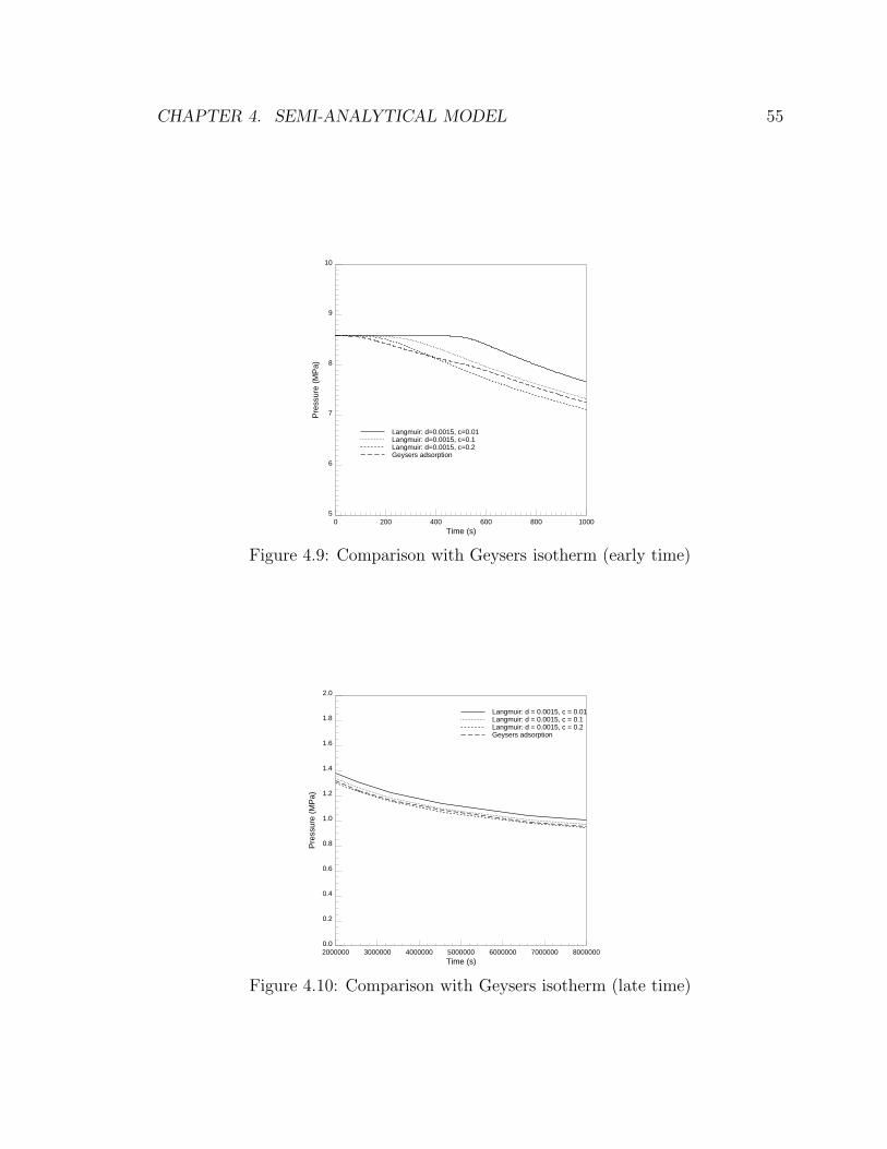
CHAPTER 4. SEMI-ANALYTICAL MODEL 55
5
6
7
8
9
10
Pre
ssur
e (M
Pa)
0 200 400 600 800 1000Time (s)
Langmuir: d=0.0015, c=0.01Langmuir: d=0.0015, c=0.1Langmuir: d=0.0015, c=0.2Geysers adsorption
Figure 4.9: Comparison with Geysers isotherm (early time)
0.0
0.2
0.4
0.6
0.8
1.0
1.2
1.4
1.6
1.8
2.0
Pre
ssur
e (M
Pa)
2000000 3000000 4000000 5000000 6000000 7000000 8000000Time (s)
Langmuir: d = 0.0015, c = 0.01Langmuir: d = 0.0015, c = 0.1Langmuir: d = 0.0015, c = 0.2Geysers adsorption
Figure 4.10: Comparison with Geysers isotherm (late time)

Chapter 5
Numerical Model
A numerical solution for flow through porous media was used to study the more com-
plex thermal effects, which are not easily studied by analytical means, and also as a
means to keep track of the fate of injected tracer. A three stage verification process
was followed in the numerical investigation. First, an isothermal material balance
was used to verify the numerical model for a fluid of constant compressibility without
adsorption. This constant compressibility model was checked against existing ana-
lytical solutions. Second, the more complicated vapor flow without adsorption effects
was simulated under both non-isothermal and isothermal conditions. Results were
compared to determine the validity of the isothermal assumption in the analytical
derivation. Third, numerical results for a wide range of adsorption isotherms were
compared to the analytical results discussed in Chapter 4 to verify accuracy of the
model for a range of reservoir conditions.
Analysis of tracer propagation for a range of reservoir adsorption conditions was
used to determine general effects of an adsorbed phase on the propagation of injected
tracer.
Numerical analysis was carried out on an example represented by a core with the
following properties:
1. Length = 4.0 m.
2. Width = 0.1 m.
56

CHAPTER 5. NUMERICAL MODEL 57
3. Height = 0.1 m.
4. Porosity = 0.05.
5. Permeability = 1.0× 10⁻¹⁶ m2 to 1.0× 10⁻¹² m2.
6. Rock Compressibility = 0.0.
7. Rock Density = 2720.0 kg/m3.
8. Initial Temperature = 300 ◦C.
9. Initial Pressure = 0.101 MPa to 7.0 MPa.
10. Production Boundary = Constant Pressure or Constant Flow Rate.
11. Outer Boundary = No Flow, Constant Pressure, or Constant Flow Rate.
Fluid properties were calculated from the National Institute for Standards and
Technology (NIST) thermophysical database for steam [26].
Numerical Solution Technique
All simulations performed in this chapter were carried out in a linear model 4 m
in length, and used grid blocks of constant height and width with the number of
grid blocks varying depending on the problem solved. The time step size also varied
depending on the size of the grid block and the maximum fluid velocity in the problem
modeled. The time step size was selected at the beginning of each simulation based
on the grid block size and the maximum velocity such that the Courant number never
exceeded 1. The Courant number is defined as:
C =uf∆t
∆x(5.1)
Thus, the constraint on time step size was based on the relationship:
C ≤ 1.0 (5.2)

CHAPTER 5. NUMERICAL MODEL 58
In each of the following sections, the discretizations in both space and time are
provided for the particular problem discussed.
Solution of the linear flow problem requires solution of a tridiagonal matrix for
pressure at each iteration level. The Thomas algorithm was employed for matrix
solution in this research. Saturation is calculated explicitly based on pressure in each
block so matrix solution for saturation was not necessary.
5.1 Single-Phase Liquid Flow Without Adsorption
Effects
The conservation equation for single-phase fluid flow through porous media is:
φ∂ρfSf
∂t+ ∇ · (ρfuf) = 0 (5.3)
Eqn. 5.3 was discretized and solved with water compressibility and viscosity
assumed constant. Darcy’s law was assumed to model the flux of fluid in a porous
media.
uf =kkrf
µf
∇p (5.4)
The discretized flow equation for a one dimensional single-phase, single component
system with constant grid block size may be written as follows for a fully implicit
formulation:
[Tfi+1/2(pfi+1 − pfi) − Tfi−1/2(pfi − pfi−1)
]ν+1 − ∆x
∆t[∆t(φfiρfiSfi)]
− qν+1fi = 0 (5.5)
where, fluid transmissibility, Tf , is defined as:
Tfi =kikrfiρfi
µfi∆x(5.6)
and the time operator, ∆t, operates as follows:
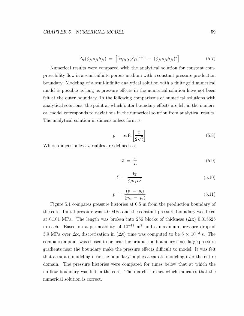
CHAPTER 5. NUMERICAL MODEL 59
∆t(φfiρfiSfi) =[(φfiρfiSfi)
ν+1 − (φfiρfiSfi)ν]
(5.7)
Numerical results were compared with the analytical solution for constant com-
pressibility flow in a semi-infinite porous medium with a constant pressure production
boundary. Modeling of a semi-infinite analytical solution with a finite grid numerical
model is possible as long as pressure effects in the numerical solution have not been
felt at the outer boundary. In the following comparisons of numerical solutions with
analytical solutions, the point at which outer boundary effects are felt in the numeri-
cal model corresponds to deviations in the numerical solution from analytical results.
The analytical solution in dimensionless form is:
p = erfc
[x
2√
t
](5.8)
Where dimensionless variables are defined as:
x =x
L(5.9)
t =kt
φµctL2(5.10)
p =(p − pi)
(pw − pi)(5.11)
Figure 5.1 compares pressure histories at 0.5 m from the production boundary of
the core. Initial pressure was 4.0 MPa and the constant pressure boundary was fixed
at 0.101 MPa. The length was broken into 256 blocks of thickness (∆x) 0.015625
m each. Based on a permeability of 10−12 m2 and a maximum pressure drop of
3.9 MPa over ∆x, discretization in (∆t) time was computed to be 5 × 10⁻³ s. The
comparison point was chosen to be near the production boundary since large pressure
gradients near the boundary make the pressure effects difficult to model. It was felt
that accurate modeling near the boundary implies accurate modeling over the entire
domain. The pressure histories were compared for times below that at which the
no flow boundary was felt in the core. The match is exact which indicates that the
numerical solution is correct.

CHAPTER 5. NUMERICAL MODEL 60
2.0
2.2
2.4
2.6
2.8
3.0
3.2
3.4
3.6
3.8
4.0
Pre
ssur
e (M
Pa)
0 20 40 60 80 100Time (S)
Numerical Solution - 256 BlocksAnalytical Solution: Comp. Error Function Soln.
Figure 5.1: Pressure histories for constant compressibility flow.
5.2 Single-Phase Vapor Flow
Single-phase vapor flow was studied under isothermal and non-isothermal conditions
and both with and without adsorption effects included. The material balance for va-
por flow with adsorption is similar to Eqn. 5.3 with an added adsorption accumulation
term.
φ∂ρvSv
∂t+ φ
∂ρaSa
∂t+ ∇(ρvuv) = 0 (5.12)
The discretized form of Eqn. 5.12 may be expressed as:
[Tvi+1/2(pvi+1 − pvi) − Tvi−1/2(pvi − pvi−1)
]ν+1 − ∆x
∆t[∆t(φviρviSvi)]
− ∆x
∆t[∆t(φaiρaiSai)] − qν+1
fi = 0 (5.13)
where the adsorbate saturation may be written in terms of an adsorption isotherm,
X(p), which relates mass adsorbed to pressure:

CHAPTER 5. NUMERICAL MODEL 61
Sai =1− φ
φ
ρai
ρrX(pi) (5.14)
Eqn. 5.13 was solved for pressure by use of an implicit finite difference scheme.
Adsorbate saturation was updated based on the iteration level pressure and was
allowed to change until the solution converged.
In all vapor flow numerical computations described in this chapter, (∆x) was
chosen to be 0.015625 m. Based on a permeability of 10−12 m2 and a maximum
pressure drop of 3.9 MPa over ∆x, discretization in (∆t) was computed to be 1 ×10⁻³ s. The relationship between ∆x and ∆t was based on the Courant number
constraint shown in Eqn. 5.2. Vapor viscosity at 2.0 MPa was used to calculate
velocity used in determining the Courant number.
A heat balance was used to calculate temperature changes in the system under
single-phase flow conditions. Temperature changes were computed explicitly and at
each iteration level. Convergence of the heat balance was required before pressure
convergence was allowed. The heat balance used (as explained in Chapter 4) was:
∂
∂t[(1− φ)ρrEr + φSvρvEv + φSaρaEa] +
∂
∂x[φSvρvEvuv]
= ∇ · (κm∇T ) + Qe (5.15)
Eqn. 5.15 neglects a number of terms which are included in the complete heat balance
(Chapter 4). Since only adsorbate and vapor phases were present, the water/vapor
phase change term was neglected but heat effects of the adsorbed phase were included.
Also, pressure work and viscous dissipation terms were neglected since they have been
shown to be small and to counteract each other [27].
5.2.1 Validity of Isothermal Flow Assumption
To simplify the the analytical description of adsorption effects as described in the
previous chapter, flow was assumed to be isothermal. In this section, numerical
solutions including thermal effects for a wide range of flow conditions were used to
determine the validity of the isothermal assumption.
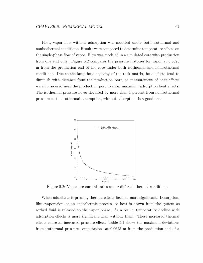
CHAPTER 5. NUMERICAL MODEL 62
First, vapor flow without adsorption was modeled under both isothermal and
nonisothermal conditions. Results were compared to determine temperature effects on
the single-phase flow of vapor. Flow was modeled in a simulated core with production
from one end only. Figure 5.2 compares the pressure histories for vapor at 0.0625
m from the production end of the core under both isothermal and nonisothermal
conditions. Due to the large heat capacity of the rock matrix, heat effects tend to
diminish with distance from the production port, so measurement of heat effects
were considered near the production port to show maximum adsorption heat effects.
The isothermal pressure never deviated by more than 1 percent from nonisothermal
pressure so the isothermal assumption, without adsorption, is a good one.
1.0
1.5
2.0
2.5
3.0
3.5
4.0
Pre
ssur
e (M
PA
)
0 50 100 150 200 250 300Time (S)
Isothermal ConditionsNonisothermal Conditions
Figure 5.2: Vapor pressure histories under different thermal conditions.
When adsorbate is present, thermal effects become more significant. Desorption,
like evaporation, is an endothermic process, so heat is drawn from the system as
sorbed fluid is released to the vapor phase. As a result, temperature decline with
adsorption effects is more significant than without them. These increased thermal
effects cause an increased pressure effect. Table 5.1 shows the maximum deviations
from isothermal pressure computations at 0.0625 m from the production end of a

CHAPTER 5. NUMERICAL MODEL 63
core with an adsorbing phase present. Thermal simulations were carried out in a
core initially near a relative pressure of 1.0. Results shown in Table 5.1 were ob-
tained using a range of adsorption isotherms which encompass all magnitudes and
shapes considered in this research. It is felt that the adsorption temperature effects
considered here include a sufficient range of isotherms that they may be considered
general. Thermal effects were shown to influence pressure depletion from a simulated
core. Pressure variations from the isothermal case were shown to range from about
4 % to a maximum of about 10 %. In general, thermal pressure effects were shown
to be large when the slope of the isotherm is large and small when the slope of the
isotherm is small. Large isotherm slopes indicate a high rate of desorption as pres-
sure is decreased which means a high rate of vaporization and a subsequent large
heat loss due to the endothermic nature of adsorption. Since thermal effects never
translated to pressure changes from isothermal conditions of more than 10 %, even
when adsorbate saturation is very large, the isothermal assumption was assumed to
be valid. Although pressure is affected by thermal effects which are not included in
the analytical solution, these effects have been shown to be very small and do not
impact the validity of the analytical results.
Results shown Table 5.1 indicate that when large amounts of adsorbed phase are
initially present, thermal effects may strongly influence the pressure depletion in a
core. For low initial adsorbed phase saturations, thermal effects on pressure depletion
are small.
In Chapter 4, the isothermal assumption was made in deriving the analytical
solution. Results shown in Table 5.1 indicate that the isothermal assumption is a
good one.
5.2.2 Comparison with Analytical Solution - Adsorbed Phase
Absent
In this section, analytical results were compared with numerical calculations for single-
phase vapor flow in the absence of a desorbing liquid phase.
Figure 5.3 shows pressure histories at 0.5 m from the production end of a test

CHAPTER 5. NUMERICAL MODEL 64
Table 5.1: Thermal Effects of Adsorbed Phase
Maximum adsorbate saturation Langmuir Maximum pressure effect(%) Shape factor (%)
33.0 0.01 7.0
33.0 1.0 5.0
33.0 100 3.5
67.0 100 10.0
67.0 100 6.5
67.0 100 5.0
core computed analytically and numerically. Vapor was produced from the production
boundary under the constraint of constant pressure (0.101 MPa). The outer boundary
was no flow for the numerical solution and infinite for the analytical solution. Initial
pressure was 8 MPa and temperature of the system was held at 300 ◦C. Permeability
was assumed to be 10−12 m2. The agreement between analytical and numerical results
is excellent. Slight disagreement at late times is due to outer boundary effects in the
numerical solution.

CHAPTER 5. NUMERICAL MODEL 65
4
5
6
7
8
9
Pre
ssur
e (M
PA
)
0 200 400 600 800 1000 1200 1400Time (S)
Analytical SolutionNumerical Solution
Figure 5.3: Analytical and numerical solutions with no adsorption
5.2.3 Comparison with Analytical Solution - Adsorbed Phase
Present
The adsorbed phase is included by using an adsorption isotherm which defines ad-
sorbed mass as a function of pressure for a given temperature. Adamson [1] showed
that adsorption isotherms may take many shapes depending on the matrix material
and pore configuration and a method of generalizing the effects is needed. Compari-
son of the numerical and analytical solutions is used to verify the numerical treatment
of adsorption effects.
Constant Adsorbed Saturation
Pressure effects of constant adsorbed saturation corresponding to chemically sorbed
liquid were computed both analytically and numerically to determine whether the
effects of the presence of adsorbate without mass transfer are accurately modeled.
Figure 5.4 shows pressure histories calculated numerically and analytically. Boundary
and initial conditions and core properties are identical to those used in the previous
section.

CHAPTER 5. NUMERICAL MODEL 66
4
5
6
7
8
9
Pre
ssur
e (M
PA
)
0 200 400 600 800 1000 1200Time (S)
Analytical: X = 0.01Numerical: X = 0.01
Figure 5.4: Analytical and numerical solutions with constant adsorption
Numerical and analytical computations shown in Figure 5.4 show excellent agree-
ment except at late times when boundary effects are felt in the numerical solution.
These results indicate that effects of the adsorbed mass without mass transfer are
modeled accurately by numerical methods.
Variable Adsorbed Saturation
The mass transfer between adsorbate and vapor also must be modeled in order to
fully quantify adsorption effects. Numerical and analytical computations were made
for pressure decline in a simulated core with an adsorbed phase present for a range of
adsorption isotherm shapes. Numerical and analytical results were compared. Figure
5.5 shows pressure histories computed analytically and numerically for vapor flow in
the presence of an adsorbed phase described by a Langmuir isotherm (d = 0.001, c
= 0.01). The numerical solution matches the analytical solution almost exactly.
The series of comparisons between analytical and numerical solutions described
above indicates that the numerical scheme used accurately calculates the pressure
response in a geothermal reservoir for all conditions of relevance.

CHAPTER 5. NUMERICAL MODEL 67
6.0
6.5
7.0
7.5
8.0
8.5
9.0
Pre
ssur
e (M
PA
)
0 200 400 600 800 1000 1200 1400Time (S)
Analytical: d = 0.001, c = 0.01Numerical: d = 0.001, c = 0.01
Figure 5.5: Analytical and numerical solutions with Langmuir adsorption
This check on the numerical results justifies the use of the numerical scheme in
determining the fate of tracer introduced into a geothermal reservoir to track tracer
flowing in the vapor phase.
5.3 Modeling Tracer Response
Modeling of the propagation of tracer is important because it highlights the different
mechanisms that control the rate at which tracer is transported by vapor in a porous
medium. The three mechanisms considered in this research were adsorption, diffusion
partitioning, and preferential partitioning. Adsorption may effect the transport of
tracer in two ways. First, if the adsorbed phase is not desorbing rapidly, it may cause
an increase in propagation rate of the vapor and of the tracer due to a reduction in the
area available for flow. Second, if the vapor carrying tracer adsorbs, the propagation
of tracer may be slowed and the concentration of tracer in the vapor phase reduced.
Thus, adsorption affects tracer propagation by affecting the transport of the fluid in
which it resides (in this research, the vapor phase).
CHAPTER 5. NUMERICAL MODEL 68
Diffusion partitioning may occur when a tracer is introduced into a porous medium
in which one or more fluids reside. Diffusion of the tracer into the resident fluid may
delay the tracer even though vapor flow rate may be unaffected or even enhanced.
Thus, diffusion partitioning may occur whether adsorption occurs or not.
Preferential partitioning occurs when the tracer properties are such that it prefer-
entially resides in one phase over another. In this research, preferential partitioning
would occur if it was shown that tritiated water (HTO) has different boiling charac-
teristics than pure water. In this chapter, the properties of T2O, HTO, and water
are studied to determine the likelihood of preferential partitioning of tritiated water
into either the liquid or vapor phase.
Each of the mechanisms for tracer delay were investigated to determine the likely
effects of each on tracer tests. To determine the effects of an adsorbed phase on tracer
production characteristics, the capability for keeping track of an injected tracer was
introduced into the numerical model.
5.3.1 Effects of Adsorption on Tracer Propagation
Since the tracer considered in this research is tritiated water which behaves very much
like water, the propagation of tracer may be modeled identically to the propagation
of a water component:
yn+1i Ti+1/2(pi+1 − pi)
n+1 − yn+1i−1 Ti−1/2(pi − pi−1)
n+1 −∆x
∆t
[(yviφviρviSvi)
n+1 + (yviφviρviSvi)n]−
∆x
∆t
[(yaiφaiρaiSai)
n+1 + (yaiφaiρaiSai)n]
+
yinjQinj − yprodQprod = 0 (5.16)
In Eqn. 5.16 pressures, saturations, and fluid properties determined at the end of
each time step in the computation of mass transport of vapor are used to compute
the mass fraction of injected mass in the vapor phase, yv in each block. To calculate
mass fraction in the vapor phase explicitly, a relation is needed between the mass
fraction in the adsorbed phase and in the vapor phase.

CHAPTER 5. NUMERICAL MODEL 69
It was assumed that the mass fraction of injected tracer in the adsorbed phase
is a weighted average of the fraction adsorbed at the old time step and the change
in adsorbed mass over the time step. In equation form, the mass fraction in the
adsorbed phase is given by:
yn+1a =
yn+1v ∆tSa + yn
aSna
Sn+1a
(5.17)
The weighted mass average for tracer concentration is important because it allows
numerical experiments to determine how adsorption of injected tracer affects the
propagation and eventual recovery of the tracer. The adsorption process is commonly
described as being a layering process in which layers of molecules of adsorbed liquid
are laid down, one on top of the other, until adsorptive forces become too weak
to hold more layers. In this static model, each layer is assumed to be stationary
in the adsorbed phase. If this model were used, it would be necessary to release the
adsorbed tracer in a layer-by-layer fashion in the reverse order of deposition. However,
adsorption is not a stationary layering process even though it may be considered
as such from a mass standpoint. In reality, adsorbed molecules are mobile in the
adsorbed phase [1], so mixing within the adsorbed phase is constantly occurring.
Thus, while adsorption of an injected tracer occurs at the concentration of tracer
in the vapor phase, desorption of tracer occurs at a diluted concentration due to
the presence of previously adsorbed liquid which mixes with adsorbed tracer. In this
section, then, the effects of tracer propagation due solely to the adsorption phenomena
are investigated. Later, the effects of diffusion and preferential partitioning will be
investigated.
Loss of injected tracer by radioactive decay was also considered in tracer compu-
tations. At the end of each time level, the total amount of injected tracer was reduced
by means of an exponential decay term:
ynf = yn
f e−kt (5.18)
For tritium, the decay constant, k, is 1.83× 10⁻⁹s−1 which gives rise to a half-life
of about 12 years. Since tritium is a long-lived conservative tracer, and most tracer

CHAPTER 5. NUMERICAL MODEL 70
tests are of short duration, decay of tritium tracer is usually negligible. In the cases
considered here, radioactive decay was immeasurably small.
A series of numerical experiments were carried out to determine the effects of
the presence of an adsorbed phase on tracer transport. These experiments were
designed to investigate all aspects of tracer transport in porous media. The effects of
initial distributions of tracer were studied. Tracer propagation under steady-state and
transient conditions were compared and the reservoir pressure at initiation of tracer
injection was varied to determine the effects of initial conditions on tracer propagation.
Finally, the effects of preferential partitioning of tracer on the propagation of injected
tritiated water were investigated.
Effects of Initial Tracer Distributions
A series of numerical experiments were carried out on a representation of one-dimensional
flow in a core at an initial pressure of 8.58 MPa and initial temperature of 300 ◦C.
These initial values of pressure and temperature correspond, approximately, to sat-
urated conditions. One end of the 4 m long core was closed and the other end was
produced at a constant pressure of 0.101 MPa. Thus, simple depletion of the core
was modeled. The core was broken into 32 blocks of length 0.125 m. In the first
series of tests, the vapor in the first block (closed end) was assumed to be tracer and
the production of this tracer from the output end of the core was computed. These
numerical tests correspond to a physical situation in which injected tracer stays en-
tirely in the vapor phase with no tracer adsorbing. A schematic of the numerical core
with assumed fluid saturations is shown in Figure 5.6. Figure 5.7 shows production
histories for a series of adsorption isotherms as compared to the production history
for tracer with no adsorbed phase present. For the numerical experiments illustrated
in Figure 5.7, the maximum adsorbed amount was assumed to be 0.001 grams of
adsorbed liquid per gram of rock.
Figure 5.8 compares the production histories for a range of isotherms with the
maximum adsorbed amount assumed to be 0.01 grams of adsorbed liquid per gram of
rock. Figures 5.7 and 5.8 both show that, in general, tracer in the vapor phase is pro-
duced more quickly when an adsorbed phase is present. Both magnitude of adsorption

CHAPTER 5. NUMERICAL MODEL 71
. . .
. . .
No Flow Boundary
Constant PressureProduction
AAAAAA
AAAAAAAAA
AAAAAA
AAAAAA
AAAAAA
AAAAAAAAA
AAAAAA
AAAAAA
Vapor Phase
AAAA
Adsorbed Phase
Tracer in the Vapor Phase
Figure 5.6: Schematic of numerical core with tracer in vapor phase.
10-10
10-9
10-8
10-7
10-6
10-5
10-4
10-3
Tra
cer
Pro
duct
ion
Rat
e (k
g/s)
0 20 40 60 80 100Time (s)
No AdsorptionLangmuir: d=0.001, c=0.01Langmuir: d=0.001, c=1.00Langmuir: d=0.001, c=100.
Figure 5.7: Tracer production histories with tracer in vapor phase.

CHAPTER 5. NUMERICAL MODEL 72
and the shape of the controlling isotherm are shown to affect tracer propagation.
10-10
10-9
10-8
10-7
10-6
10-5
10-4
10-3
Tra
cer
Pro
duct
ion
Rat
e (k
g/s)
0 20 40 60 80 100Time (s)
No AdsorptionLangmuir: d=0.01, c=0.01Langmuir: d=0.01, c=1.00Langmuir: d=0.01, c=100.
Figure 5.8: Tracer production histories with tracer in vapor phase.
Figure 5.7 shows accelerated tracer breakthrough for concave down (c = 100)
isotherms and a delay in tracer breakthrough for concave up (c = 0.01) and linear
(c = 1) isotherms. As pressure is depleted from the far end of the core, desorption
occurs to replace the produced mass and, simultaneously, vapor from the closed end
of the core begins to flow toward the pressure sink. When an immobile adsorbed
phase is present, vapor is forced to flow through a smaller area and, therefore, vapor
flow velocity is increased for a given pressure drop. For concave down isotherms, the
mass replacement due to desorption is not rapid enough to overcome the increased
flow rate of vapor due to a decreased flow path, and tracer propagation is increased.
For linear isotherms, the two effects almost cancel and breakthrough times are not
strongly altered. For concave up isotherms desorption mass replacement becomes
dominant so pressure depletion in the vapor phase is slowed and tracer propagation
is slowed as well.
Figure 5.8 shows the same general effects as described above in Figure 5.7. How-
ever, since adsorption mass is greater in the system shown in Figure 5.8, the mass

CHAPTER 5. NUMERICAL MODEL 73
effects of adsorption are magnified.
In a second series of numerical experiments, tracer was assumed to exist, initially,
only in the adsorbed phase in the block nearest the no flow boundary (Figure 5.9).
Fluid was produced from the other end of the core at a constant pressure of 0.101 MPa.
Figure 5.10 shows production rate histories for a series of isotherms when tracer was
assumed to initially reside in the adsorbed phase. Both mass adsorbed and the shape
of the adsorption isotherms were shown to alter the production history of tracer. For
comparison purposes, since mass adsorbed varies with the Langmuir magnitude factor,
d, the concentration was altered so initial mass in place was equal. As when tracer
was confined to the vapor phase, concave up isotherms (c < 1) cause delays in tracer
breakthrough for a given adsorbed mass. Comparison of tracer production controlled
by isotherms having the same shape but with different magnitudes of adsorbed mass
show that increased adsorbed mass also contributes to the production delay, but does
not have a strong influence on the shape of the tracer production.
. . .
. . .
No Flow Boundary
Constant PressureProduction
AAAAAA
AAAAAAAAA
AAAAAA
AAAAAA
AAAAAA
AAAAAAAAA
AAAAAA
AAAAAA
Vapor Phase
AAAA
Adsorbed Phase
AATracer in the Adsorbed Phase
Figure 5.9: Schematic of numerical core with tracer in adsorbed phase.
Preliminary investigations indicate that the presence of an adsorbed phase can
have a number of effects on propagation of tracers through porous media. Depending
on the shape of the controlling isotherm, the pressure of the system, preferential phase

CHAPTER 5. NUMERICAL MODEL 74
10-10
10-9
10-8
10-7
10-6
10-5
10-4
10-3
10-2
Tra
cer
Pro
duct
ion
Rat
e (k
g/s)
0 20 40 60 80 100Time (s)
Langmuir: d=0.001, c=0.01Langmuir: d=0.001, c=1.00Langmuir: d=0.01, c=0.01Langmuir: d=0.01, c=1.00
Figure 5.10: Tracer production histories with tracer in adsorbed phase.
residence of the tracer, the production characteristics of tracer can be significantly
altered. To determine the likely effects of an adsorbed phase on propagation of
injected tracer, a series of numerical experiments were carried out in which a slug of
tracer was injected into a core and transport of the tracer was calculated. A range
of initial conditions, controlling isotherms, and injection and production rates were
used.
Steady-State Flow
In the following series of numerical representations of slug tests, both injection and
production rates were held constant at 0.01 kg/s. Injection and production were
allowed to continue without introduction of tracer until steady state conditions were
obtained. When steady state flow was reached, a 0.001 kg slug of tracer was injected.
The tracer propagation is shown in Figure 5.11 as a series of tracer concentration
profiles in the vapor phase. Numerical runs were carried out for a series of adsorption
isotherms and were compared. Results show that for steady state conditions, diffusion
of the tracer is not strongly affected by the presence of an adsorbed phase, but
convection of the tracer can be significantly increased by an adsorbed phase relative

CHAPTER 5. NUMERICAL MODEL 75
to convection in the absence of an adsorbed phase. Diffusion is not strongly influenced
because, under steady state conditions, neither adsorption nor desorption is occurring,
so no fluid retardation is taking place. Only linear isotherms are highlighted in Figure
5.11 because, since no adsorption nor desorption is taking place, the shape factor of
the isotherm does not influence the propagation of tracer. The magnitude factor of
the isotherm, however, does affect tracer propagation, although these effects are not
large. Comparison of tracer profiles at 21 seconds for isotherms with d = 0.001 and
d = 0.01 indicate that a ten-fold increase in adsorbed mass causes a two-fold increase
in vapor phase velocity. Therefore, while adsorbed mass does affect steady-state
propagation of tracer, these effects are considered small.
0.0
0.2
0.4
0.6
0.8
1.0
Mas
s F
ract
ion
of T
race
r in
Vap
or P
hase
0.0 0.5 1.0 1.5 2.0 2.5 3.0 3.5 4.0Distance from Injector (m)
Time = 20s: No AdsorptionTime = 21s: No AdsorptionTime = 20s: Langmuir: d=0.001, c=1.0Time = 21s: Langmuir: d=0.001, c=1.0Time = 20s: Langmuir: d=0.01, c=1.0Time = 21s: Langmuir: d=0.01, c=1.0
Figure 5.11: Tracer profiles for steady state conditions.
Transient Flow
In the next series of slug tests, the core initial pressure was set at 5.0 MPa and a
0.001 kg slug of tracer was injected upon initiation of injection so transient adsorption
effects could be studied. Injection and production rates were both 0.01 kg/s. Figure
5.12 shows tracer propagation in the core under these transient conditions.
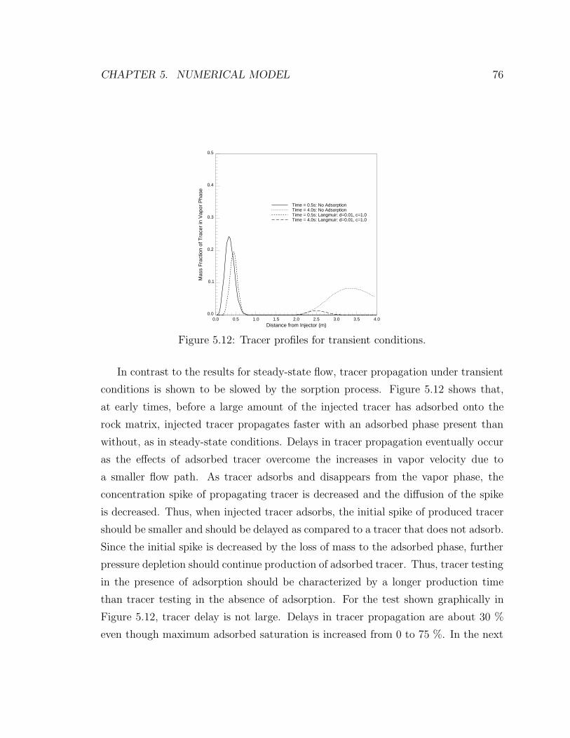
CHAPTER 5. NUMERICAL MODEL 76
0.0
0.1
0.2
0.3
0.4
0.5
Mas
s F
ract
ion
of T
race
r in
Vap
or P
hase
0.0 0.5 1.0 1.5 2.0 2.5 3.0 3.5 4.0Distance from Injector (m)
Time = 0.5s: No AdsorptionTime = 4.0s: No AdsorptionTime = 0.5s: Langmuir: d=0.01, c=1.0Time = 4.0s: Langmuir: d=0.01, c=1.0
Figure 5.12: Tracer profiles for transient conditions.
In contrast to the results for steady-state flow, tracer propagation under transient
conditions is shown to be slowed by the sorption process. Figure 5.12 shows that,
at early times, before a large amount of the injected tracer has adsorbed onto the
rock matrix, injected tracer propagates faster with an adsorbed phase present than
without, as in steady-state conditions. Delays in tracer propagation eventually occur
as the effects of adsorbed tracer overcome the increases in vapor velocity due to
a smaller flow path. As tracer adsorbs and disappears from the vapor phase, the
concentration spike of propagating tracer is decreased and the diffusion of the spike
is decreased. Thus, when injected tracer adsorbs, the initial spike of produced tracer
should be smaller and should be delayed as compared to a tracer that does not adsorb.
Since the initial spike is decreased by the loss of mass to the adsorbed phase, further
pressure depletion should continue production of adsorbed tracer. Thus, tracer testing
in the presence of adsorption should be characterized by a longer production time
than tracer testing in the absence of adsorption. For the test shown graphically in
Figure 5.12, tracer delay is not large. Delays in tracer propagation are about 30 %
even though maximum adsorbed saturation is increased from 0 to 75 %. In the next
CHAPTER 5. NUMERICAL MODEL 77
series of tests, the magnitude of this production delay is studied for a wide range of
adsorption isotherms and initial conditions.
Effects of Initial Condition
A series of slug tests was designed to investigate the influence of initial conditions on
the transient effects of tracer sorption. These tests were used to illustrate the mag-
nitude of tracer delay by adsorption, the amount of dispersion associated with tracer
propagation, and the combined effects of initial pressure and adsorption isotherm on
propagation of tracer. For all runs in this section, isotherms used were described by a
Langmuir model with d = 0.01. The Langmuir shape factor, c, was varied from 0.01
to 100.0. Initial conditions in the core were then varied. Injection was described by
a constant pressure boundary set to a maximum of 2 MPa greater than initial pres-
sure and production was described by a constant pressure boundary of 0.101 MPa
(atmospheric conditions). In all runs described in this section, the injection well was
switched to production after tracer breakthrough at the production well. By compar-
ing the the tracer production histories for the producer and the converted injector,
conclusions are reached about the propagation of injected tracer for a range of initial
conditions.
In the first test, the initial pressure was set at 7.0 MPa. This condition corresponds
to initiation of tracer injection very early in the production life of a reservoir. Figure
5.13 shows the tracer rate histories at the production well for a series of isotherms.
Clearly, both the adsorbed mass and the shape of the describing isotherm affect tracer
propagation. When the isotherm is concave down (c = 100.0) nearly maximum adsor-
bate saturation is reached before initiation of injection. Therefore, the injected tracer
is forced to flow through a smaller effective channel and, as a result breakthrough
occurs more quickly and the concentration of produced tracer is higher. For concave
up isotherms (c = 0.01) most of the adsorption occurs at pressures higher than 7 MPa
for a reservoir at 300 ◦C so the breakthrough time is not strongly affected. However,
subsequent adsorption of injected tracer reduces the concentration of tracer in the
production stream.

CHAPTER 5. NUMERICAL MODEL 78
10-8
10-7
10-6
10-5
10-4
10-3
Tra
cer
prod
uctio
n ra
te (
kg/s
)
0 10 20 30 40 50Time (s)
No adsorbed phaseLangmuir; d = 0.01, c = 0.01Langmuir; d = 0.01, c = 100.
Figure 5.13: Tracer production for early initiation of injector.
In the second test, the initial pressure was set at 4.0 MPa. This condition cor-
responds to initiation of injection half way through the production life of a reservoir
which starts at saturated conditions. Figure 5.14 shows the tracer rate histories at
the production well for a range of conditions. For concave down (c = 100) isotherms,
the breakthrough of tracer is accelerated compared to a no adsorption case since ad-
sorbate saturation reduces the flow path area available for vapor flow. Initiation of
injection at 4 MPa does not allow significant adsorption which might increase the
diffusion of the produced tracer spike. Similarly, breakthrough of tracer for concave
up (c = 0.01) isotherms is also accelerated relative to a no adsorption case for the
reasons described above. In neither case is the magnitude of the adsorption spike
significantly affected since very little adsorption or desorption takes place.
In the third test, the initial pressure was set at 0.101 MPa. This condition corre-
sponds to initiation of tracer injection very late in the productive life of a reservoir
which starts at saturated conditions. Figure 5.15 shows the tracer rate histories at the
production well for a range of isotherms when injection is carried out at a constant
pressure of 2.101 MPa. For strongly concave down isotherms (c = 100), no tracer

CHAPTER 5. NUMERICAL MODEL 79
10-8
10-7
10-6
10-5
10-4
10-3
Tra
cer
prod
uctio
n ra
te (
kg/s
)
0 10 20 30 40 50Time (s)
No adsorbed phaseLangmuir; d = 0.01, c = 0.01Langmuir; d = 0.01, c = 100.
Figure 5.14: Tracer production for midlife injection initiation.
breaks through at the production well due to the large rate of adsorption of injectate
at low pressures. For concave up isotherms (c = 0.01), the tracer production response
is almost identical in shape to the no adsorption case but the magnitude is reduced
slightly and the breakthrough is slightly retarded due to the adsorption of a small
amount of injectate.
For the tracer production runs shown in Figures 5.13 through 5.15, tracer effects
are shown to depend on the conditions at which injection of tracer is initiated. Only
for cases of injection initiation very late in the life of the reservoir are adsorption
delay effects shown to occur.
For the initial conditions described above, a second set of runs were made in which
the injector was switched to a producer upon breakthrough of tracer at the production
well. Figures 5.16, 5.17, and 5.18 show the subsequent production of tracer from the
converted injection well for initial reservoir pressures of 8 MPa, 4 MPa, and 0.101
MPa, respectively.

CHAPTER 5. NUMERICAL MODEL 80
10-8
10-7
10-6
10-5
10-4
10-3
Tra
cer
prod
uctio
n ra
te (
kg/s
)
0 20 40 60 80 100Time (s)
No adsorbed phaseLangmuir; d = 0.01, c = 0.01Langmuir; d = 0.01, c = 100.
Figure 5.15: Tracer production for late initiation of injector.
10-10
10-9
10-8
10-7
10-6
10-5
10-4
10-3
Pro
duct
ion
rate
of i
njec
ted
trac
er (
kg/s
)
0 20 40 60 80 100Time (s)
No AdsorptionLangmuir: d=0.01, c=0.01Langmuir: d=0.01, c=100.0
Figure 5.16: Tracer production from injector (pi = 8 MPa).

CHAPTER 5. NUMERICAL MODEL 81
10-10
10-9
10-8
10-7
10-6
10-5
10-4
Pro
duct
ion
rate
of i
njec
ted
trac
er (
kg/s
)
0 20 40 60 80 100Time (s)
No AdsorptionLangmuir: d=0.01, c=0.01Langmuir: d=0.01, c=100.0
Figure 5.17: Tracer production from injector (pi = 4 MPa).
10-10
10-9
10-8
10-7
10-6
10-5
Pro
duct
ion
rate
of i
njec
ted
trac
er (
kg/s
)
0 20 40 60 80 100Time (s)
No AdsorptionLangmuir: d=0.01, c=0.01Langmuir: d=0.01, c=100.0
Figure 5.18: Tracer production from injector (pi = 0.101 MPa).

CHAPTER 5. NUMERICAL MODEL 82
5.3.2 Effects of Diffusion Partitioning on Tracer Propagation
To determine the likelihood of diffusion partitioning of tracer, investigations must be
carried out about the sizes of the diffusive flux and the convective flux of the tracer
in a given porous medium. In many reservoirs, the diffusive flux of a tracer in one
dimension is described by the following form of Fick’s Law:
vdiff = −Dmol∂C
∂x(5.19)
In Eqn. 5.19, vdiff represents the diffusional flux of tracer, Dmol is the molecular
diffusivity of the tracer, and the gradient of tracer concentration is expressed by
∂C/∂x. Fick’s law is written for diffusion in a bulk liquid and molecular diffusivities
are generally expressed in terms of bulk liquid in the absence of a porous medium.
When a porous medium is present, the diffusivity is decreased due to tortuosity of the
porous medium. The diffusivity of tritiated water through water is reported by Leap
[40] to be about 2.3 ×10⁻⁵cm2/s. However, in a porous medium, the diffusivity is
expected to be much lower. In a porous medium, both the porosity and the tortuosity
of the medium cause a reduction in the diffusivity. In very small pores for which the
pore radius approaches the mean free path of the liquid molecule, the diffusivity is
reduced even further. Geankoplis [29] reports that the diffusivity coefficient in porous
medium is related to the bulk phase diffusivity by the following relationship:
Dpore = Dbulk
[φ
a2
](5.20)
where, a is the actual pore length per distance in the direction of diffusion.
Eqn. 5.20 shows that the porous media diffusivity is a function of the porosity, φ,
and the tortuosity (denoted by a) of the porous media. In many geothermal reservoirs,
especially the Geysers, there are two types of porosity, fracture and bulk. It is usually
assumed that flow occurs in the fractures and storage in the form of condensed and
adsorbed liquid occurs in the bulk porosity matrix. Figure 5.19 shows a schematic of
the porosity in a geothermal reservoir.
Porosities reported by Gunderson [32] show that porosity for a large region of
reservoir in the Geysers is around 5 %. However, much of the total porosity is from

CHAPTER 5. NUMERICAL MODEL 83
AAAAAAAAAAAAAAAAAAAAAAAAAAAAAAAAAAAAAAAAAAAAAAAAAAAAAAAAAAAAAAAAAAAAAAAAAAAAAAAAAAAAAAAAAAAAAAAAAAAAAAAAAAAAAAAAAAAAAAAAAAAAAAAAAAAAAAAAAAAAAAAAAAAAAAAAAAAAAAAAAAAAAAAAAAAAAAAAAAAAAA
Widely distributed vugs and intergranular voids.
AAConcentration of vugs and intergranular voids near fracture.
AA Mineralized fracture.
Vugs within mineralized fracture.
Young fracture.
Figure 5.19: Schematic of porosity in a geothermal reservoir.
fracture porosity and a very small portion comes from the interparticle porosity of
the system. Gunderson [32] also points out that fractures are usually separated by
several centimeters. Therefore, when tracer is injected into a geothermal reservoir,
it preferentially flows in the vapor phase in the fractures, but diffuses into the in-
terparticle porosity along the fractures (Figure 5.19). Based on the description of
Geysers porosity provided by Gunderson [32] and the diffusion model in Eqn. 5.20
an estimate of the diffusivity of tritiated water into the matrix surrounding fractures
was computed. Making the conservative assumptions that interparticle porosity is 1
%, and that the measure of pore tortuosity, a, is 2, the diffusivity of tritiated water
is estimated to be 5.8 ×10⁻¹⁰ m2/s.
The diffusivity of tritiated water into the porous matrix and the permeability of
the porous medium were then used to evaluate the relative sizes of the convective
and diffusive terms to determine whether diffusion partitioning is significant at the
Geysers.
Assuming that bulk flow occurs in fractures and adsorbed liquid is stored in smaller
CHAPTER 5. NUMERICAL MODEL 84
pores surrounding the fracture (an assumption consistent with observed pore distribu-
tions in many geothermal reservoirs) diffusion into the porous matrix was compared
with convection in the fracture. Eqn. 5.19 was used with the diffusivity of tritiated
water computed as above to calculate the rate at which tritiated water diffuses into
a 1 cm long pore with a maximum concentration gradient. In other words, the diffu-
sive flux computed for the maximum concentration gradient was used so a maximum
diffusive flux was computed. The maximum diffusion rate was found to be 5.8×10⁻⁸
m/s. If Darcy’s law is assumed to approximate the flow rate in the fractures, convec-
tion rates ranging from 2.9× 10⁻⁵ to 2.9× 10⁻⁹ m/s were computed for the range of
permeabilities measured at the Geysers. Thus, except in extremely low permeability
regions, the convective flux is significantly greater than the diffusive flux. Further-
more, since only a maximum diffusive flux was used in the comparison, it is probable
that the time to reach a concentration equilibrium between a tracer in flowing vapor
and adsorbed liquid by diffusion alone is much too large for the assumption of instan-
taneous concentration equilibrium between vapor and adsorbed liquid to be valid for
the range of permeability at the Geysers. However, for the lower permeable portions
of the reservoir, the equilibrium assumption is probably valid, so investigation of the
effects of diffusion partitioning is necessary. So, for permeabilities in the range 10−15
- 10−16 m2, the assumption of instantaneous concentration equilibrium between the
vapor and adsorbed liquid is probably true in the Geysers. An analytical solution
for tracer convection, dispersion, and diffusion partitioning was derived based on a
similar derivation by Antunez [5]. The purpose of deriving this analytical solution
is to isolate the effects of diffusion partitioning of tracer into adsorbed liquid. Pre-
viously, the effects of adsorption were isolated from diffusion effects and were shown
to be small. Here, the effects of diffusion are isolated from adsorption effects. The
following assumptions were made for the derivation:
1. The adsorbed phase is immobile.
2. The vapor and adsorbed phase saturations are constant. This assumption sep-
arates the effects of diffusion from those of adsorption.
3. The tracer partitions instantly and equally between vapor and adsorbed liquid
CHAPTER 5. NUMERICAL MODEL 85
phases by diffusion.
4. The formation is homogeneous and isotropic.
5. Flow is linear.
6. Dispersion is proportional to the local velocity: K = |v|
In a derivation analogous to that of Antunez [5], the mass conservation equation
for tracer propagating in a porous medium was found to be:
∂2C
∂x2− uv
K
∂C
∂x=
(Svρv + Saρa
KρvSv
)∂C
∂t(5.21)
Eqn. 5.21 was solved with the following initial and boundary conditions:
C(x, t = 0) = 0 (5.22)
C(x = 0, t) = Co (5.23)
C(x →∞, t) → ∞ (5.24)
After manipulation, the final form of the equation may be written: (for detailed
derivation, the reader is referred to Antunez [5])
C(x, t)
Co=
1
2exp
[xuv
K
]erfc
x√
Svρv+Saρa
KSvρv
2√
t−
uv
K
√t
2√
Svρv+Saρa
KSvρv
+1
2exp
[xuv
K
]erfc
x√
Svρv+Saρa
KSvρv
2√
t+
uv
K
√t
2√
Svρv+Saρa
KSvρv
(5.25)
At late time, the second term in Eqn. 5.25 becomes negligible, so under these
conditions, the solution for tracer concentration reduces to:
C(x, t)
Co
=1
2exp
[xuv
K
]erfc
x√
Svρv+Saρa
KSvρv
2√
t−
uv
K
√t
2√
Svρv+Saρa
KSvρv
(5.26)

CHAPTER 5. NUMERICAL MODEL 86
In Eqns. 5.25 and 5.26, uv refers to the steady state vapor velocity, C stands for
the concentration of tracer, and K denotes the dispersion coefficient. In order to use
the equations, their validity in geothermal reservoirs was tested. Volumetric flow rate
was modeled by Darcy’s law for single-phase flow.
qsc =kATscp
µzTpsc
dp
dx(5.27)
For a pressure drop between the reservoir, pe, and the well, pw, Eqn. 5.27 may be
written:
qsc =kATsc
µzTpsc
p2e − p2
w
2(xe − xw)(5.28)
which may be rearranged to the following form:
qsc =kATsc
µzT pscp
pe − pw
(xe − xw)(5.29)
In Eqn. 5.29, p is the arithmetic average reservoir pressure while µ and z are
calculated at the root mean square average pressure. These assumptions have been
shown to be valid by Brigham [11] as long as there are not large variations in reservoir
pressure or fluid properties.
The Geysers reservoir was chosen as a model for determining the effects of diffusion
partitioning in tracer transport. Reservoir properties from sources cited throughout
this report have been used in the following computations. An average pressure of
3.325 MPa was computed from a far-field pressure of 3.9 MPa and a well pressure
of 2.75 MPa. Average values of viscosity and compressibility factor were found to
be 1.76 ×10⁻⁵ Pa·s and 0.86, respectively. Over the pressure range considered, the
viscosity varied by 1 % and the compressibility factor varied by 5% so the model
assumed for the computation of vapor velocity is valid (Eqn. 5.29).
It was shown above that diffusion effects become large with respect to convection
only for permeabilities on the order of 10−15 - 10−16 m2. Therefore, this range was
used in computing the volumetric flux of vapor. For the range in permeabilities used,
the volumetric flux of vapor varies from 4 ×10⁻⁶ to 4 ×10⁻⁷ m3/m2 · sThe velocity, computed as:
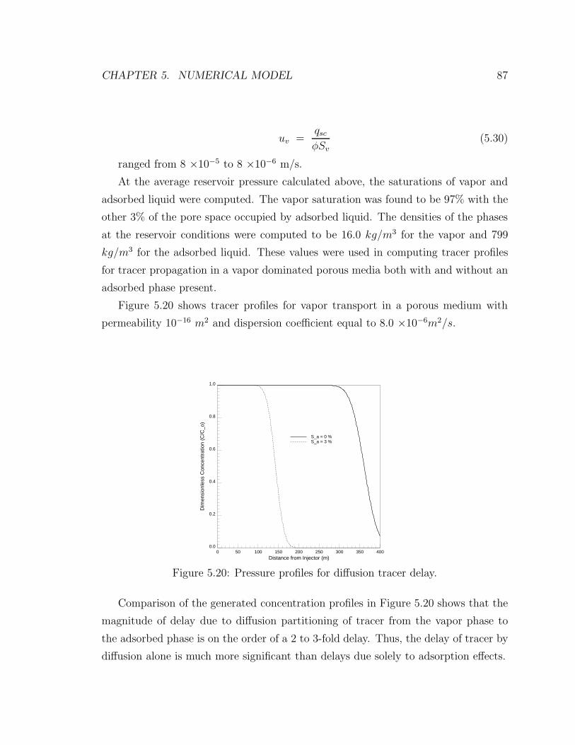
CHAPTER 5. NUMERICAL MODEL 87
uv =qsc
φSv(5.30)
ranged from 8 ×10⁻⁵ to 8 ×10⁻⁶ m/s.
At the average reservoir pressure calculated above, the saturations of vapor and
adsorbed liquid were computed. The vapor saturation was found to be 97% with the
other 3% of the pore space occupied by adsorbed liquid. The densities of the phases
at the reservoir conditions were computed to be 16.0 kg/m3 for the vapor and 799
kg/m3 for the adsorbed liquid. These values were used in computing tracer profiles
for tracer propagation in a vapor dominated porous media both with and without an
adsorbed phase present.
Figure 5.20 shows tracer profiles for vapor transport in a porous medium with
permeability 10−16 m2 and dispersion coefficient equal to 8.0 ×10⁻⁶m2/s.
0.0
0.2
0.4
0.6
0.8
1.0
Dim
ensi
onle
ss C
once
ntra
tion
(C/C
_o)
0 50 100 150 200 250 300 350 400Distance from Injector (m)
S_a = 0 %S_a = 3 %
Figure 5.20: Pressure profiles for diffusion tracer delay.
Comparison of the generated concentration profiles in Figure 5.20 shows that the
magnitude of delay due to diffusion partitioning of tracer from the vapor phase to
the adsorbed phase is on the order of a 2 to 3-fold delay. Thus, the delay of tracer by
diffusion alone is much more significant than delays due solely to adsorption effects.

CHAPTER 5. NUMERICAL MODEL 88
5.3.3 Effects of Preferential Partitioning on Tracer Propaga-
tion
One of the main problems in using tracers to determine flow characteristics in porous
media is that, often, tracers do not behave exactly like the fluid they are designed to
track. In geothermal reservoirs, tritium is a commonly used tracer. It is used because,
in the form in which it is carried through water (HTO), its characteristics are almost
identical to those of water for a range of conditions [45]. However, even given the
similarities between tritiated water and ordinary water, partitioning is often cited as
a possible explanation for tracer diffusion during injection tests.
Greenkorn [30] and Deem, et. al. [18] showed that adsorption of tritiated water
by sandstone is of the same order as would be expected for water. In determining
the partitioning of tritiated water between the vapor and liquid phases, the control-
ling characteristics are the temperature-pressure relationship of the tracer and the
density of the tracer. If the temperature-pressure characteristics of the tracer are
significantly different than the liquid it is designed to track, the tracer will boil at dif-
ferent reservoir conditions and will, therefore partition differently between the liquid
and vapor. If the densities of the tracer and tracked liquid are significantly different,
the heavier liquid will preferentially tend to remain in the liquid phase even if boiling
characteristics of the fluid are similar. Matsunaga and Nagashima [46] showed that,
for a range of temperatures from 20 to 300 ◦C, the vapor pressure of T2O varied by
a maximum of 2.5 % from pure water values. Also, for temperatures below 180 ◦C,
T2O is actually more likely to partition into the vapor phase than the liquid phase
based upon the temperature-pressure characteristics of the fluid. In vapor dominated
reservoirs, temperatures are well above saturated conditions so boiling partitioning
should not occur at all.
The density of gaseous T2O was shown to be different than steam at temperatures
likely in geothermal reservoirs. In the range of temperatures found in the Geysers (230◦C - 250 ◦C) the density of T2O is 20 % greater than steam. It is sometimes assumed
that the density differences between water and tritiated water will cause tritiated
water to partition into the liquid phase. However, the saturation curve described

CHAPTER 5. NUMERICAL MODEL 89
above clearly shows that the boiling characteristics of T2O are almost identical to
those of water. Thus, while the density of tritiated water in the liquid and vapor form
may be up to 20 % larger than for water, the boiling characteristics are unaffected
by the density differences of the liquids.
When using tritium as a tracer in geothermal reservoirs, it is introduced into the
reservoir in the form of tritiated water, not as T2O. Since there is only one tritium
atom in a molecule of HTO, the boiling characteristics of tritiated water are even
closer to water than are those of T2O. So, since the boiling properties of tritiated
water are almost identical to those of water, it may be concluded that tritiated water
tracer does not tend to move into either the liquid or vapor phase in preference
to water. Therefore, preferential partitioning does not influence the propagation of
tracer.
Chapter 6
The Geysers Geothermal Reservoir
The Geysers geothermal field is the largest developed geothermal resource in the
world. It is located in the Mayacmas range about 120 kilometers north of San Fran-
cisco near Santa Rosa, California (Figure 6.1). The Geysers field lies in dry, moun-
tainous terrain and is characterized by several areas of surface thermal activity.
The Geysers field was discovered in 1847 and commercial use of the hot surface
waters in spas began in the 1860’s. Production of Geysers steam for generation of
electricity began in the 1920’s with the drilling of eight shallow wells between 1921
and 1925. The wells were drilled to depths of 60 to 190 m and steam pressures of
1.0 to 2.1 MPa were encountered. The development resulted in the generation of 35
kW of electrical power which was used by a local resort spa. The project had many
problems and was abandoned in the early 1930’s.
No further development of the Geysers took place until 1955 when modern devel-
opment of the field began. Large scale development began in the 1960’s and continued
at an accelerated rate until the late 1980’s when steep pressure decline in the field
curtailed development. Geysers energy production peaked in the late 1980’s at a gross
capacity of about 2200 MWe. Reddy and Goldemberg [62] estimate that the energy
needs of an average American home are about 1 kW so energy production from the
Geysers supports the equivalent of about 2.2 million homes. Therefore, the Geysers
represents a significant energy resource.
Barker, et. al. [7] summarized the growth in generation capacity at the Geysers
90
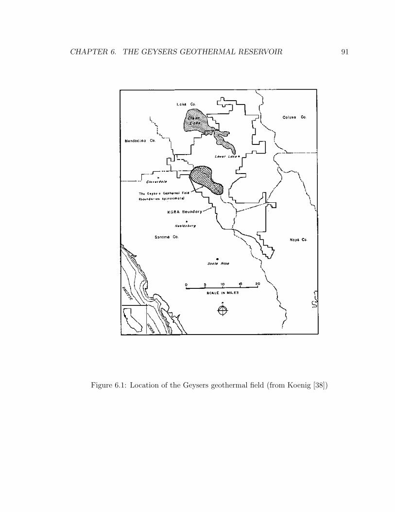
CHAPTER 6. THE GEYSERS GEOTHERMAL RESERVOIR 91
Figure 6.1: Location of the Geysers geothermal field (from Koenig [38])

CHAPTER 6. THE GEYSERS GEOTHERMAL RESERVOIR 92
as occurring in three phases:
1. Phase I: From 1960 to 1968, 82 MW of generation capacity was added at an
average of 10 MW per year.
2. Phase II: From 1969 to 1981, 861 MW of generation capacity was added at an
average of 67 MW per year.
3. Phase III: From 1982 to 1988, 861 MW of generation capacity was added at
an average of 150 MW per year.
The accelerated rate at which the Geysers has been developed has had an effect
on the production decline in the field. In approximately 1987, during Phase III
development, listed above, well production decline rates began to steepen. Figure
6.2 (from Barker, et. al. [7]) shows mass production and net electrical generation for
leases held by UNOCAL, Magma Power Co. and Thermal Power Co. (UMT). For the
period shown in Figure 6.2, UMT leases accounted for almost all of the production
at the Geysers. Field flow rate and electrical generation decline are shown to occur
at 1987.
Figure 6.2: Geysers production (from Barker, et. al. [7])
The seemingly obvious reason for fieldwide production decline is that over pro-
duction has resulted in an increase in decline rate. However, it is not clear that

CHAPTER 6. THE GEYSERS GEOTHERMAL RESERVOIR 93
extrapolation at decline rates currently experienced will yield accurate production
forecasts. The proven existence of an adsorbed phase may significantly alter the pro-
duction decline of the reservoir even if production is maintained at current levels. By
characterizing the pressure effects of an adsorbed phase in geothermal reservoirs, the
general depletion characteristics of a geothermal reservoir are determined. Then, by
applying general results to known adsorptive characteristics at the Geysers, long-term
effects of adsorption on depletion at the Geysers may be determined.
In Chapter 4, the general depletion effects of an adsorbed phase in a geothermal
reservoir are shown. In Chapter 5, the general effects of an adsorbed phase on the
injection and subsequent production of a tracer are highlighted. In this chapter,
the effects of an adsorbed phase on depletion and the simultaneous injection and
production at the Geysers geothermal reservoir are studied by making use of field
data.
6.1 Geysers Reservoir Properties
The Geysers reservoir is heterogeneous and there is a large range in properties over
the reservoir. A number of studies have attempted to determine Geysers reservoir
properties and the range of values is shown in Table 6.1.
The reservoir properties listed in Table 6.1 include data sampled at widely sep-
arated portions of the field, and at widely varying times. These values, however,
provide a framework within which adsorption effects at the Geysers can be analyzed.
In numerical experiments carried out in this chapter, reservoir properties are varied
within the ranges presented above to determine the likely fate of injected tracer.

CHAPTER 6. THE GEYSERS GEOTHERMAL RESERVOIR 94
Table 6.1: Geysers Reservoir Properties
Property Range of Values
Pressure [7] 1.2 - 3.6 MPa
Temperature [72] [21] 230 - 250 ◦C
Porosity [32] 0.6− 5.8%
Permeability [7] 5× 10⁻¹⁸ − 1.8× 10⁻¹³ m2
Rock Density [21] [65] 2650 - 2720 kg/m3
Rock Thermal Conductivity [69] 1.26 - 3.60 W/(m ◦ C)
Rock Heat Capacity [34] 1.30× 10³ kJ/(m3 ◦C)
CHAPTER 6. THE GEYSERS GEOTHERMAL RESERVOIR 95
6.2 Injection at the Geysers
The method of cooling tower condensate disposal and mass replacement in the Gey-
sers has been injection of surface water and condensed produced vapor. To assess the
effectiveness of the injection program, knowledge of the fate of injected fluid is neces-
sary. In particular, the information necessary for evaluation of an injection program
includes knowledge of injector/producer connectivity and the potential for recharge
of the Geysers adsorbed liquid.
Connectivity between an injector and producer determines the velocity with which
injected fluid will travel between the injector and producer. As the fluid velocity
increases and the distance between the injector and producer decrease, the residence
time of the fluid decreases resulting in reduced heat transfer to the injected fluid and
a reduced exploitation of heat reserves.
Recharge of the adsorbed liquid through injection is accomplished by increas-
ing reservoir pressure and increasing the adsorbed mass as dictated by the porous
medium’s characteristic adsorption isotherm.
A method for keeping track of injected fluids is to inject a tracer along with the
injectate; and, by recording subsequent production of tracer in surrounding wells,
information on well connectivity and recharge potential may be inferred. Gulati, et.
al., [31] pointed out five objectives in running a tracer survey:
1. To determine if any of the injected water is vaporizing.
2. To determine how much of the injected water is being produced as steam at the
nearby production wells.
3. To determine the regional flow pattern of fluid in the reservoir.
4. To determine if the efficiency of water vaporization is declining or staying con-
stant with time.
5. To determine if the regional flow pattern will undergo a substantial change when
new units go on stream.

CHAPTER 6. THE GEYSERS GEOTHERMAL RESERVOIR 96
To these five objectives, a sixth may be added which may hold great significance
for production from the Geysers and other geothermal reservoirs.
6. To determine the effects of vapor adsorption on the production delay of injected
fluid.
Gulati, et. al., [31] go on to point out necessary characteristics of the tracer used
to meet the six objectives listed above. The characteristics related to the physical
properties of the tracer are:
1. It should not be adsorbed on the rocks.
2. Its phase should change only when the phase of the injected water changes.
3. When liquid with a certain concentration of tracer vaporizes, both vapor and
liquid should have the same tracer concentration. [i.e. the tracer should not
preferentially partition into either the vapor or liquid phase.]
4. The half life of tracer (if radioactive) should be more than one year because
significant quantities might appear at production wells for a year or more.
In light of current evidence that liquid adsorption occurs to a fairly significant
degree in Geysers reservoir rock, the first characteristic listed above should be altered
to “It should not tend to adsorb to a greater degree than the phase in which it
resides”. In other words, an injected tracer should not selectively partition into any
of the liquid phases present in the reservoir. An analysis carried out in Chapter 5
show that preferential partitioning effects are insignificant and may be ignored.
Finally, the half-life of tritium is about 12.5 years, thus it is a conservative tracer
which does not decay appreciably over the life of most tracer tests.
The data summarized above indicates the following properties for tritiated water
(HTO):
1. HTO does not adsorb on solid surfaces to a greater degree than water. There-
fore, preferential adsorption of HTO will not occur in reservoir tracer tests.

CHAPTER 6. THE GEYSERS GEOTHERMAL RESERVOIR 97
2. Since the vapor pressure curve for HTO is nearly identical to that of water, the
vaporization characteristics of HTO can be considered to be the same as those
of water. Also, since phase partitioning is dependent upon the vaporization
characteristics of a given fluid, partitioning is shown to be insignificant.
3. Most tracer tests last far less than 12.5 years, so the radioactive decay of tritium
is usually negligible.
The characteristics of tritium tracer, therefore, are ideally suited to tracer analysis
in geothermal reservoirs. An analysis of the effects of adsorption on propagation of an
injected tracer was carried out within the context of the six objectives listed above.
Results of tracer analysis were used to determine the effects of mass replacement due
to injection.
6.2.1 History of Injection at the Geysers
In 1991, UNOCAL prepared a summary of injection projects carried out at the Gey-
sers. The report is an excellent source for information about the history of injection
at the Geysers and future plans for injection. For the remainder of this chapter, un-
less otherwise referenced, injection information is taken from the UNOCAL injection
report [68]. A detailed map of the Geysers geothermal field showing operators of the
field and the location of power generation plants (Figure 6.3) is provided by Barker,
et. al. [7]. Unit locations roughly coincide with the location of power generation
plants. Figure 6.3 is used as a reference for well locations throughout the rest of this
chapter.
Reinjection of cooling tower condensate began at the Geysers in 1969 with an
injection to production ratio of 5 %. At initiation of the injection program, all
injectate was cooling tower condensate. In 1980, fresh water injection, extracted
from Big Sulphur Creek, was initiated into the Units 1-6 area. A second fresh water
facility began providing fresh water for injection in 1983. Fresh water injection peaked
at 7 % in 1983 while total injection (including condensate) has stayed fairly constant
at 20 - 25 % since the early 70’s.
CHAPTER 6. THE GEYSERS GEOTHERMAL RESERVOIR 98
Figure 6.3: Unit location at the Geysers (from Barker, et. al. [7])
CHAPTER 6. THE GEYSERS GEOTHERMAL RESERVOIR 99
In general, two injection strategies have been used at the Geysers – deep injection
and shallow injection. In deep injection, outlying wells with deep steam entries are
used as injectors to minimize downward channeling of liquid water to nearby wells.
Effects of deep injection are often difficult to quantify and while some short term ben-
efits have been observed, it has been assumed that most of the benefits are long term
[68]. The shallow injection strategy uses injection wells with steam entries higher
than surrounding wells and relies on the vaporization of injected water as it chan-
nels toward surrounding production wells. Since breakthrough of shallow injectate
is usually fairly rapid, benefits of shallow injection are generally short term. In the
following sections, specific injection operations at the Geysers, for which data was
collected, are described and the future of injection is discussed.
Unit 17 Injection
Injection into the Unit 17 area at the Geysers began in March, 1988, through well
DX-72. Unit 17 injection was a deep injection project so effects were expected to be
long term. In 1991, surrounding well rates were analyzed to determine the effects of
injection. Wells DX-28 and DX-64 experience increased flow rates by 8 kilopounds
per hour (kph) each and each well experienced a reduction in decline rate. Decline
rate reduction in DX-28 was between 12.5% and 9.6% while decline rate reduction in
DX-64 was about 12.5%. Wells DX-63 and DX-23 experienced temporary production
increases, but decline rates were not altered on a long term basis.
Based on the production responses described above, effects of deep well injection
were shown to have slight short-term effects (rate increase of 10 kph), and slightly
greater long term flow rate effects (increases of 16 kph). Slight long term decline rate
effects were also observed (decline rate reduction of 4%).
Unit 14 Injection
Another deep injection project was undertaken in the Unit 14 area of the Geysers
field. The project was initiated in 1983 with injection of condensate and fresh water
into GDCF 117A-19, GDC-18, and GDC-1. By 1987, production and thermal decline
CHAPTER 6. THE GEYSERS GEOTHERMAL RESERVOIR 100
in the reservoir indicated that injection should be curtailed. From 1987 through
1989, injection was limited to GDCF 117A-19 to allow the area to recover thermally.
Following thermal recovery, low pressure, high heat conditions were evident in the
Unit 14 area and injection was restarted in GDC-18. While high injection rates were
maintained, a positive production response was noticed in offset wells but a lack of
injection water reduced the effectiveness of the injection program. By 1992, only 10%
of injectate had been recovered, but analysis of the injection program is continuing.
Unit 9-10 Injection
Injection at a rate of 500 gpm into LF-2 began on February 14, 1992. This injection
program represented UNOCAL’s first shallow injection project and was expected to
produce short term results. Within two months of injection, seven offset production
wells showed production increases totaling a 6% return of injected condensate. The
nearest producer, LF-39, watered out very quickly after its early production increases
and was shut-in. The Unit 9-10 injection program is currently being monitored for
further injection effects.
Low Pressure Area Injection
Enedy, et. al. [22] described an injection project in the southeast Geysers. Data used
in this section is from their report.
On September 20, 1989, a large scale injection program was initiated in the south-
east Geysers with injection into C-11 [22] (Figure 6.4).
Although C-11 experienced several shut-in periods, production at about 800 gpm
was maintained until June 4, 1990 when a five month shut-in period ensued. Injection
was restarted for 8 days on August 8, 1990 and the test was concluded in November,
1990. Injection was directed at a Low Pressure Area (LPA) which was characterized
by a low reservoir pressure (<1.5 MPa) and a high reservoir temperature (230 ◦C).
Injection rate into C-11 is shown in Figure 6.5.
A total of 2 billion (9.1 × 10⁸ kg) of condensate was injected into the LPA via
C-11. The injection program had two major effects. First, reservoir pressure in the
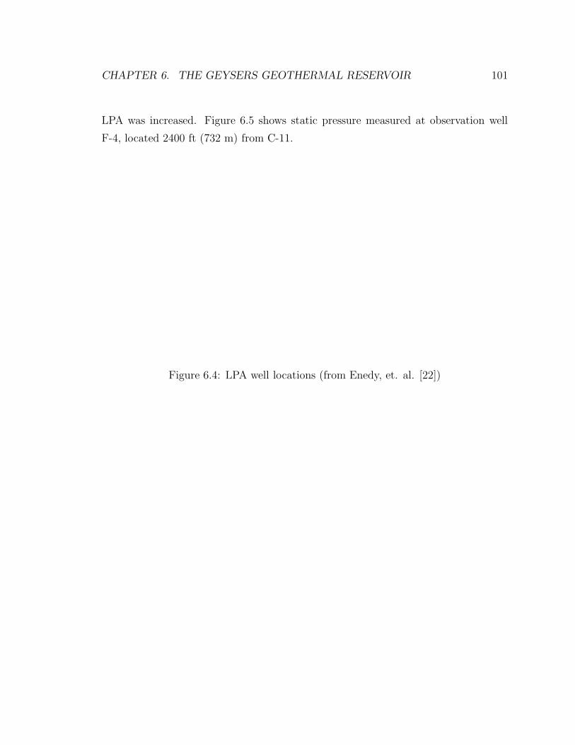
CHAPTER 6. THE GEYSERS GEOTHERMAL RESERVOIR 101
LPA was increased. Figure 6.5 shows static pressure measured at observation well
F-4, located 2400 ft (732 m) from C-11.
Figure 6.4: LPA well locations (from Enedy, et. al. [22])

CHAPTER 6. THE GEYSERS GEOTHERMAL RESERVOIR 102
Figure 6.5: F-4 observation well pressures (from Enedy, et. al. [22])

CHAPTER 6. THE GEYSERS GEOTHERMAL RESERVOIR 103
Second, the injection program resulted in increases in both mass and energy pro-
duction rate. Figure 6.6 shows monthly production rates for wells owned by the three
operators in the LPA. Wells owned by Calpine were declining at a 25 % rate before
injection began but soon after injection, production rates began to incline at a 58 %
rate. UNOCAL wells, declining at 5 % before injection, went on a 21 % incline after
injection. And, NCPA wells switched from a 35 % decline to a 61 % incline due to
the C-11 injection program.
Figure 6.6: LPA monthly flowrate (from Enedy, et. al. [22])
A 20 MW increase in steam production within 5 months of injection was noted by
Enedy, et. al. [22]. Thus, heat extraction was increased due to injection into C-11.
The LPA injection program demonstrated that injection can be used as a means
to increase production from the Geysers reservoir and increase the efficiency of heat
extraction from the reservoir. An analysis of the LPA injection project in terms of
adsorbed mass replacement is carried out later in this chapter.
The Future of Injection at the Geysers
Design of future injection projects at the Geysers will depend on the results of earlier
injection projects and on results from research aimed at understanding the effects of
injection on recharge.
CHAPTER 6. THE GEYSERS GEOTHERMAL RESERVOIR 104
Currently, operators at the Geysers are considering numerous injection options but
uncertainty about the usefulness of injection makes decisions about these programs
difficult. Under consideration are injection programs using ground water, surface
water, treated waste water, and cooling tower condensate. Ground water extraction
from the Cobb Mountain and Clear Lake volcanics is being considered as a possible
water supplement for injection at the Geysers and extraction programs and costs are
currently being evaluated.
Surface water is another possible source of injection water at the Geysers. Several
water sources, Kelsey Creek, Putah Creek, and Big Sulphur Creek, are currently being
considered for development as water sources. High costs and difficulties in obtaining
water rights present obstacles to these sources.
UNOCAL, Lake County, Calpine, NCPA, and PG&E are currently considering
construction of a pipeline to transport treated waste water to the Geysers from Lake
County. As with ground water and surface water sources, costs of treated waste water
are high and may prove to be too expensive for use at the Geysers.
Currently, most of the injected water at the Geysers comes from cooling tower
condensation. Between 20% and 25% of produced water is collected and reinjected.
Projects for increasing condensate recovery efficiency are costly and it is doubtful
that it will be economically possible to increase injection of cooling tower condensate.
Uncertainty about development of injection programs is due, in large part, to
uncertainties about the usefulness of water injection at the Geysers. While ongoing
field studies are being used to further determine the observable short term effects
of injection, the current research is aimed at determining the long term effects due
to adsorption. During injection of water, pressure increases in the reservoir lead to
an increase in the adsorbed mass. Determination of the magnitude of this added
adsorbed mass is useful in determining the long term storage and production effects
of an injection program. To quantify the recharge of adsorbed mass at the Geysers,
field pressure data and tracer production data were used.

CHAPTER 6. THE GEYSERS GEOTHERMAL RESERVOIR 105
6.2.2 Effects of Injection on Adsorbate Recharge
Based on data gathered in the LPA injection test, estimates of the recharge of the
adsorbed mass in the Geysers geothermal reservoir due to injection were prepared
in this study. An overview of the LPA is shown in Section 6.2.1. Enedy, et. al.
[22] analyzed test data to determine the potential for reinjection to increase reservoir
pressure and increase steam production. However, they did not analyze the potential
for recharge of adsorbed mass. In this section, data from the LPA injection test is
used to estimate the recharge of adsorbed mass accomplished in a typical injection
project.
In the LPA injection test, reservoir pressures, as measured at the wellhead in ob-
servation well F-4, increased from 1.03 MPa at the initiation of injection to 1.31 MPa
at the end of the test. Assuming an average reservoir temperature of 230 ◦C, the rel-
ative pressure was increased from 0.3685 to 0.4687. Based on the Geysers adsorption
isotherm shown in Section 2.3.1, Figure 2.5, this increase in pressure corresponds to
an increase in adsorbed mass from 0.15 mg/g to 0.18 mg/g. Thus, the adsorbed mass
was increased by 0.03 mg/g.
Enedy, et. al. [22] reported the area of the LPA as 790 acres or 3.2 × 10⁶ m2.
Open well intervals were reported in three wells in the LPA. Open hole thickness in
well 956A-2 was reported as 975 m, in well F-6 as 1036 m, and in well C-11 as 1933 m.
Assuming a reservoir thickness of 2000 m and assuming that the entire thickness of
the reseroir is available for flow, an effective LPA volume of 6.4 × 10⁹ m3 is obtained.
Rock density was assumed to be 2.72 × 10⁶ g/m3. Based on the volume of rock and
the rock density, the mass of rock in the LPA is 1.74 × 10¹⁶ g. It was shown above
that the amount of increase of adsorbed mass based on the F-4 well pressure rise is
0.03 mga/gr. Assuming the pressure rise was uniform in over the LPA, the increase
in adsorbed mass is computed as 5.2 × 10¹¹ g.
Total mass injected into the LPA through injector C-11 was reported by Enedy,
et. al. [22] as about 2 billion pounds or 9.1 × 10¹¹ g. Thus, using the mass adsorbed
shown above, the estimated mass adsorbed is about 57 % of the total mass injected.
The above calculations, while approximate, indicate that the mass adsorbed in an
injection project at the Geysers may be a large fraction of the injected mass.
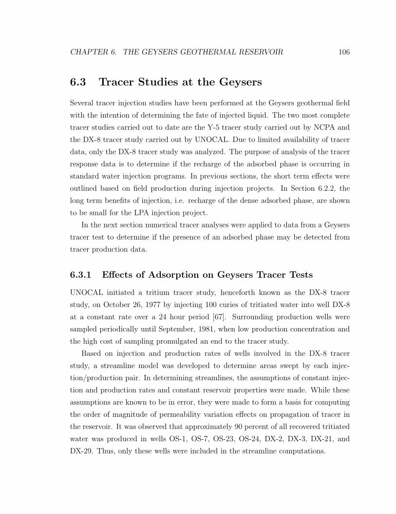
CHAPTER 6. THE GEYSERS GEOTHERMAL RESERVOIR 106
6.3 Tracer Studies at the Geysers
Several tracer injection studies have been performed at the Geysers geothermal field
with the intention of determining the fate of injected liquid. The two most complete
tracer studies carried out to date are the Y-5 tracer study carried out by NCPA and
the DX-8 tracer study carried out by UNOCAL. Due to limited availability of tracer
data, only the DX-8 tracer study was analyzed. The purpose of analysis of the tracer
response data is to determine if the recharge of the adsorbed phase is occurring in
standard water injection programs. In previous sections, the short term effects were
outlined based on field production during injection projects. In Section 6.2.2, the
long term benefits of injection, i.e. recharge of the dense adsorbed phase, are shown
to be small for the LPA injection project.
In the next section numerical tracer analyses were applied to data from a Geysers
tracer test to determine if the presence of an adsorbed phase may be detected from
tracer production data.
6.3.1 Effects of Adsorption on Geysers Tracer Tests
UNOCAL initiated a tritium tracer study, henceforth known as the DX-8 tracer
study, on October 26, 1977 by injecting 100 curies of tritiated water into well DX-8
at a constant rate over a 24 hour period [67]. Surrounding production wells were
sampled periodically until September, 1981, when low production concentration and
the high cost of sampling promulgated an end to the tracer study.
Based on injection and production rates of wells involved in the DX-8 tracer
study, a streamline model was developed to determine areas swept by each injec-
tion/production pair. In determining streamlines, the assumptions of constant injec-
tion and production rates and constant reservoir properties were made. While these
assumptions are known to be in error, they were made to form a basis for computing
the order of magnitude of permeability variation effects on propagation of tracer in
the reservoir. It was observed that approximately 90 percent of all recovered tritiated
water was produced in wells OS-1, OS-7, OS-23, OS-24, DX-2, DX-3, DX-21, and
DX-29. Thus, only these wells were included in the streamline computations.

CHAPTER 6. THE GEYSERS GEOTHERMAL RESERVOIR 107
Streamline model
In developing the streamline model, the following assumptions were made:
1. Steady-state conditions prevail.
2. The line source approximation may be used to determine pressure at a point in
the reservoir (i.e. flow is two-dimensional).
3. Total mass injected exactly balances total mass produced.
4. Fluid velocity may be calculated by Darcy’s law.
While production and injection rates of the wells considered in this study varied
over the period of interest, average rates were determined from early time data.
Production rates of the 8 production wells were summed and the average injection
rate was subtracted from this total. The remaining injection rate was assumed to
come from outside the study area. In order to introduce fluids from the surrounding
area, 12 imaginary wells were positioned around the study to provide the excess mass.
Table 6.2 lists the rates used in computing streamlines and the percentage of tracer
recovered from the production well.
Figure 6.7 shows a schematic of well locations used to develop the DX-8 stream-
lines.
Streamlines were computed in a stepwise fashion by use of the following procedure:
1. An injector is chosen as a basis for computing streamlines. In this case, DX-8
was chosen.
2. A series of flow vectors are assumed to leave the injector for a range of angles.
These angles are chosen as a starting point for tracking injected fluid particles
and are completely arbitrary. The length of the flow vector is small so the
streamline is smooth.
3. Starting at the end of the initial arbitrary flow vector, the pressure gradients
in the x and y directions are calculated from the derivative of the exponential

CHAPTER 6. THE GEYSERS GEOTHERMAL RESERVOIR 108
Table 6.2: Well Production Data
Well Name Flow Rate Tracer Recovered(kg/s) (% of total recovered)
DX-8 -43.4 0.0
OS-1 12.6 19.05
OS-7 13.5 3.52
OS-23 17.4 33.74
OS-24 20.0 10.79
DX-2 8.7 7.29
DX-3 5.6 7.64
DX-21 8.3 3.77
DX-29 13.5 2.38
integral solution. Pressure derivatives are calculated for the sum of all wells in
the system.
4. The resulting pressure gradient at the point in the reservoir is used to calculate
the velocity for the next flow vector.
5. Using the velocity and the predetermined vector length, a new small flow vector
is drawn.
6. This process is repeated over small steps until the head of a vector coincides with
the coordinates of a production well at which point the streamline is complete.
Figure 6.8 shows developed streamlines for the DX-8 tracer study.

CHAPTER 6. THE GEYSERS GEOTHERMAL RESERVOIR 109
Imaginary WellInjector Producer
DX-8
OS-1
OS-23
OS-24
OS-7
DX-3
DX-29
DX-2
DX-21
100 m
Figure 6.7: Schematic of well placement for streamline generation.
OS-1
OS-23
OS-24
OS-7
DX-3 DX-29
DX-2DX-21
100 m
Figure 6.8: DX-8 tracer study streamlines.

CHAPTER 6. THE GEYSERS GEOTHERMAL RESERVOIR 110
Computation of Tracer Propagation
A numerical computation of tracer response for the DX-8/OS-23 well pair on com-
puted stream tubes for that well pair was used to demonstrate the effects of adsorption
on tracer response at the Geysers. Tracer production was simulated both with and
without an adsorbed phase present. Simulations were carried out with the numeri-
cal model discussed in Chapter 5. Figure 6.9 shows computed stream tubes for the
DX-8/OS-23 well pair. The stream tubes were computed as described in the previous
section.
OS-23
DX-8
100 m
Figure 6.9: Streamlines for DX-8/OS-23 well pair.
Each stream tube shown in Figure 6.9 was approximated by a linear flow path.
Each stream tube length was computed as the mid-tube length between injector
and producer. The average width of each tube was computed by assuming unit
thickness in each tube, computing the volume of the tube, and then constructing
linear approximations of each tube with a constant width such that the volume of
the tube remained constant. After linearizing each tube, individual tube data was
computed as shown in Table 6.3. The height of the linearized stream tubes was
computed by matching the initial breakthrough time of the tracer. By using a trial

CHAPTER 6. THE GEYSERS GEOTHERMAL RESERVOIR 111
method, it was found that using a height of 1 m, initial breakthrough time of the
tracer was closely matched if a permeability of 5.8 × 10⁻¹⁵ m2 was used in tube
number 10 (Table 6.3). The breakthrough time can also be matched by simultaneously
increasing the permeability and block height. However, since little information on
the thickness of the permeable region is known and the permeability is within the
reported permeability range in the Geysers (Table 6.1), a 1 m block height was used
in all numerical simulations.
For all numerical calculations performed in this chapter, the space dimension was
broken into 100 blocks. Thus, in the shortest tube, the block thickness (∆x) was
about 3.5 m while in the longest tube, ∆x was about 4.7 m. In order to ensure that
the Courant number did not exceed 1, a maximum velocity was computed based on
Geysers data. Using a maximum permeability of 10−12 m2, a maximum pressure drop
across a block of 1.15 MPa, and a minimum block thickness of 3.5 m, a maximum
time step of about 200 s was computed. In all simulations carried out in this section,
a time step of 100 s was used.
Production data and details about sampling were provided by UNOCAL [67].
Production rate and tracer production data for well OS-23 are summarized in Table
A.1. Production rates and concentration of radioactive tracer were measured at the
well-head. Steam samples were taken from a vent on the well, condensed, stored in a
6 ml bottle and sent in for analysis. A Hewlett-Packard Model 3375 Tricarb Liquid
Scintillation Spectrometer was used to measure the amount of radioactivity in the
sample. The rate of radioactivity produced from the well is computed by use of the
following equation:
1 count/(min · 6 ml) = 3.4954× 10⁻⁸ ×G (µCi/s) (6.1)
where the production rate, G, is specified in units of lb/hr. Based upon Eqn. 6.1,
the radioactivity production rate of from well OS-23 is shown in Figure 6.10.
The mass concentration of tritium in the OS-23 production stream was calcu-
lated by use of the following relationship between radioactivity of tritium and its
concentration in water:

CHAPTER 6. THE GEYSERS GEOTHERMAL RESERVOIR 112
Table 6.3: OS-23 Stream tube data.
Tube Number Mid-Tube Length (m) Average Width (m)
1 405.1 7.1
2 385.6 6.6
3 374.3 6.5
4 365.9 6.4
5 359.7 5.9
6 355.2 6.1
7 352.4 6.0
8 351.1 5.9
9 351.4 6.1
10 353.1 5.6
11 356.4 6.2
12 361.4 6.5
13 368.3 6.5
14 377.1 6.3
15 388.2 7.0
16 401.8 7.3
17 418.5 7.1
18 439.3 8.1
19 465.8 8.6

CHAPTER 6. THE GEYSERS GEOTHERMAL RESERVOIR 113
3.2× 10⁻¹² Ci
1.0 kg water=
3 atoms T
1018 atoms H(6.2)
Use of tabulated mass production rates, Qm, and concentration production, Qc,
may be used to determine the radioactive concentration on a mass basis, Rc:
Rc
[Ci
kg
]= Qc
[Ci
s
]/Qm
[kg
s
](6.3)
Eqn. 6.2 may be used to determine the mass fraction of tritium tracer in the
produced water at a given point in time. These data transformations were performed
on radioactivity production data for well OS-23 and the results are shown in Figure
6.11. The figure represents tracer concentration at the production well without the
influences of a variable production rate included. These concentration values may be
used to model tracer transport in the reservoir.
0.0
0.1
0.2
0.3
0.4
0.5
Tra
cer
prod
uctio
n ra
te (
µCi/s
)
0 200 400 600 800 1000 1200 1400Time (Days post injection)
Figure 6.10: Tritium production from OS-23 (from UNOCAL [67])
A series of numerical runs were made to determine the propagation of tracer from
the injection well, DX-8, to the production well, OS-23. Since it is known that per-
meability varies widely in the Geysers (see Table 6.1), a range of permeabilities were

CHAPTER 6. THE GEYSERS GEOTHERMAL RESERVOIR 114
10-4
10-3
10-2
10-1
Tra
cer
conc
entr
atio
n (g
/g)
0 200 400 600 800 1000 1200 1400Time (Days post injection)
Figure 6.11: Mass concentration of produced tritium (from UNOCAL [67])
used in the generated stream tubes to determine if transmissibility effects can explain
the long tail in tracer production response. Additionally, since variable permeability
results in a variation in flow rates through the tubes, constant pressure boundary
conditions were selected so tubes with high permeability would receive more injected
fluid than tubes with lower permeability. Barker, et. al. [7] showed that reservoir
pressure in the DX-8 area at initiation of the injection program ranged from about 2.0
MPa in the southwest section of the study area to just under 3.5 MPa in the northeast
section. Based on this data, an average initial pressure of 2.75 MPa was assumed for
the well pair studied. By 1981, at the completion of the tracer test, pressures ranged
from 1.7 MPa in the southwest, to 3.1 MPa in the northeast. Injection pressure was
assumed to be approximately the saturation pressure at 250 ◦C, 3.9 MPa, and the
production pressure was assumed to remain constant at 1.0 MPa. Unfortunately, the
injection rate was not closely monitored during the injection of tracer, so the injec-
tion concentration is unknown. The concentration was assumed, therefore to be 1.0
and breakthrough concentrations were then normalized to the initial breakthrough
concentrations measured in the DX-8 study.

CHAPTER 6. THE GEYSERS GEOTHERMAL RESERVOIR 115
Based on the initial and boundary conditions described above and using the range
of permeabilities shown in Table 6.1, a series of runs were made assuming the largest
permeability in the center tube (tube 10) and decreasing permeability outward (to-
ward tubes 1 and 19). Figure 6.12 shows the composite concentration of tritium at
the production block for the stream tube model shown in Figure 6.9. Two sets of
runs were made; one with adsorption effects and one without. Comparison of the
two computed concentration curves shows that adsorption has very minor effects on
tracer propagation. Figure 6.12 indicates that tracer velocity is slightly increased
since very little adsorption of tracer occurs near the injector and very little pres-
sure support from desorption occurs near the producer. Clearly, the delay in tracer
transport shown in Figure 6.11 can be easily explained in terms of permeability an
geometric variation.
10-4
10-3
10-2
10-1
Tra
cer
Con
cent
ratio
n
0 200 400 600 800 1000 1200 1400Time (Days post injection)
Measured concentrationsComputed concentrations - Without adsorptionComputed concentrations - With adsorption
Figure 6.12: Mass concentration of producted tritium (stream tube model)
Based on the minor influences an adsorbed phase was shown to have on the prop-
agation of tracer in Chapter 5, it is clear that the injected fluid delay can be affected
much more strongly by permeability variations than by the presence of an adsorbed
phase.

Chapter 7
Conclusions
Conclusions about the effects of an adsorbed phase in geothermal reservoirs in general
and in the Geysers geothermal reservoir in particular are summarized below.
1. It has been shown that the density of adsorbed liquid residing in geothermal
reservoirs may be significantly lower than the density of saturated liquid water
at the same temperature. In pores filled with adsorbed liquid, density of the
adsorbed liquid may be as small as 70 % of the density of saturated liquid. It
has been shown that this pore filling adsorption phenomena almost certainly
occurs in geothermal reservoirs.
2. Based upon pore size distributions in a geothermal reservoir, the saturations of
capillary dominated and adsorption dominated liquid can be determined.
3. Using pore size distributions from the Geysers geothermal reservoir, it has been
shown that, while adsorbed phase density may be significantly different from
saturated liquid density, the volume occupied by adsorbed liquid is sufficiently
small that no significant differences in liquid saturation estimates are caused.
4. Based on the pore size distribution and adsorption isotherm characterizing a
porous medium, the density of the retained liquid phase may be determined as
a function of pressure. This data may be used in modeling.
116

CHAPTER 7. CONCLUSIONS 117
5. It was shown that the heat of vaporization in the Geysers geothermal reservoir
can vary from the value at saturated conditions to about 1.5 times that value
in very small pores.
6. Variations in heat of vaporization in the Geysers are shown to be largely due
to the adsorption of liquid molecules and not due to surface stretching or liquid
compression phenomena.
7. Due to low volumes represented by very small pores, it was concluded that at
the Geysers, values of both the heat of vaporization of adsorbed liquid water and
the internal energy may be assumed to be their values at saturated condition
for modeling purposes with little loss of accuracy.
8. The assumption of instantaneous thermal equilibrium in a geothermal reservoir
was shown to be valid in the presence of adsorption. For fracture-like pores of
width up to 1 mm, thermal equilibrium is almost instantaneous.
9. The heat transfer rate between rock and injected liquid is shown to be affected
slightly by the presence of an adsorbed phase. Heat transfer may be increased
by 15 % by the presence of an adsorbed phase. Thus, with an adsorbed phase
present, the validity of the thermal equilibrium assumption is enhanced.
10. By using a range of Langmuir isotherms, it was demonstrated that the nonlinear
effects of an adsorbed phase on pressure depletion in a geothermal reservoir are
due to the rate of change of mass stored and not on the value of the mass stored.
Thus, pressure support is obtained when the slope of the controlling isotherm
is large regardless of the mass adsorbed.
11. Real gas pseudopressure and the pseudotime may be used along with a simi-
larity analysis to solve for adsorption pressure effects in a geothermal reservoir.
The highly nonlinear partial differential equation describing such flow can be
simplified to a nonlinear ordinary differential equation.
12. Initial pressure drawdown and the rate of pressure depletion have been shown
to be significantly affected by the presence of an adsorbed phase. Time to initial

CHAPTER 7. CONCLUSIONS 118
pressure drawdown may be delayed by an order of magnitude by an adsorbed
phase.
13. By use of a measured adsorption isotherm from the Geysers, it has been shown
that pressure depletion effects may be modeled closely using a Langmuir ad-
sorption model.
14. The isothermal flow assumption used in deriving the analytical solution was
shown to be valid for low porosity geothermal systems. A wide range of adsorbed
masses and adsorption isotherm shapes were tested.
15. The effects of adsorption on tracer propagation were shown to be dependent on
isotherm shape and initial conditions. A flat isotherm over the range of pressures
experienced during injection of tracer results in very small influences on tracer
propagation. Tracer transport may even be increased due to the presence of
an adsorbed phase. At most, tracer delays due to adsorption were shown to be
about 30 %.
16. Diffusion partitioning of tritated water tracer was shown to significantly delay
the propagation of injected tracer. For a 3 % adsorbed phase saturation, tracer
transport was shown to be 2 to 3 times slower than when no adsorbed phase
was present.
17. Since the saturation curve for T2O is nearly identical to that of ordinary water,
it was concluded that preferential partitioning of tritium does not occur in vapor
dominated reservoirs. Preferential partitioning refers to partitioning into either
the vapor or liquid phases due to differences in boiling characteristics.
18. Estimates of recharge of the adsorbed phase during injection at the Geysers
indicate that a large fraction of injected fluid becomes adsorbed liquid.
19. Permeability variations were shown to have much larger effects on tracer prop-
agation than adsorption, diffusion partitioning of tracer, or preferential parti-
tioning of tracer.

Nomenclature
English Variables
Variable Description Units
A Nonlinear term dimensionlessc Compressibility 1/kPac Langmuir shape factor dimensionlessC Heat capacity kJ/kg · ◦Cd Langmuir magnification factor dimensionlessE Internal energy kJ/kgh Enthalpy kJ/kgk Permeability mdK Thermal conductivity kJ/s · m · ◦CL Characteristic length mn Number of moles dimensionlessp Pressure bar
119
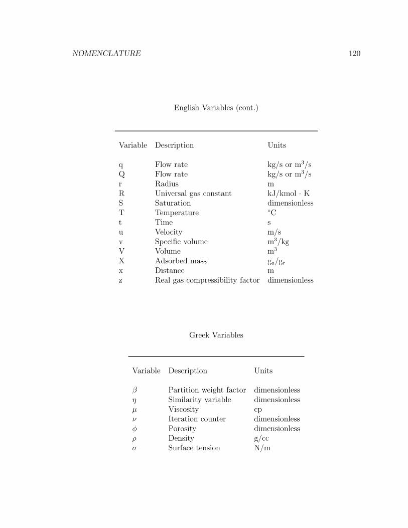
NOMENCLATURE 120
English Variables (cont.)
Variable Description Units
q Flow rate kg/s or m3/sQ Flow rate kg/s or m3/sr Radius mR Universal gas constant kJ/kmol · KS Saturation dimensionlessT Temperature ◦Ct Time su Velocity m/sv Specific volume m3/kgV Volume m3
X Adsorbed mass ga/gr
x Distance mz Real gas compressibility factor dimensionless
Greek Variables
Variable Description Units
β Partition weight factor dimensionlessη Similarity variable dimensionlessµ Viscosity cpν Iteration counter dimensionlessφ Porosity dimensionlessρ Density g/ccσ Surface tension N/m
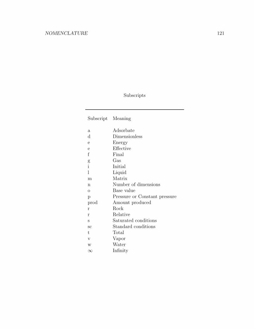
NOMENCLATURE 121
Subscripts
Subscript Meaning
a Adsorbated Dimensionlesse Energye Effectivef Finalg Gasi Initiall Liquidm Matrixn Number of dimensionso Base valuep Pressure or Constant pressureprod Amount producedr Rockr Relatives Saturated conditionssc Standard conditionst Totalv Vaporw Water∞ Infinity

NOMENCLATURE 122
Conversion Factors
Units Conversion Multiplier Units
g × 2.205× 10−3 = lbg/cm3 × 32.17 = lb/ft3
J × 9.481× 10−4 = Btum × 3.281 = ftm2 × 1012 = Darcym3 × 35.31 = DarcyN × 0.2248 = lbPa × 1.45× 10−4 = psiPa × 9.9931× 10−6 = barPa × 9.869× 10−6 = atmPa s × 999.60 = cpW s × 3.413 = BTU/hr

Bibliography
[1] Adamson, A. W.: Physical Chemistry of Surfaces, fifth edition, John Wiley &
Sons, Inc. (1990).
[2] Agarwal, R. G.: “Real Gas Pseudo-Time – A New Function for Pressure Buildup
Analysis of MHF Gas Wells,” paper SPE 8279 presented at the 1979 SPE Annual
Meeting, Las Vegas, NV, Sept., 23-26.
[3] Al-Hussainy, R., Ramey, H. J., Jr., and Crawford, P. B.: “The Flow of Real
Gases Through Porous Media,” J. Pet. Tech., Trans., AIME (May 1966) No.
237, 637–642.
[4] Anbarci, K. and Ertekin, T.: “A Simplified Approach for In-Situ Characteri-
zation of Desorption Properties of Coal Seams,” paper SPE 21808 presented at
the 1991 Rocky Mountain Regional Meeting and Low-Permeability Reservoirs
Symposium, Denver, April 15-17.
[5] Antunez, E. U.: Semi-Analytic Approach to Analyze Single Well Tracer Tests,
PhD dissertation, Stanford University (1984).
[6] Aziz, K. and Settari, A.: Petroleum Reservoir Simulation, Applied Science
(1979).
[7] Barker, B. J., Gulati, M. S., Bryan, M. A., and Riedel, K. L.: “Geysers Reservoir
Performance,” Geothermal Resources Council Transactions, Vol. 13 (1989) 349–
367.
123

BIBLIOGRAPHY 124
[8] Bhatia, S. K.: “Modeling the Pore Structure of Coal,” AIChE Journal (1987)
33, No. 10, 1707–1718.
[9] Blazek, C. F., Jasionowski, W. J., and Tiller, A. J.: “Charge/Discharge Char-
acteristics of High-Capacity Methane Adsorption Storage Systems,” Proceed-
ings: 25th Intersociety Energy Conversion Engineering Conference – IECEC ’90,
IEEE, IEEE Service Center (Aug 1990) 306–314.
[10] Bojan, M. J., Vernov, A. V., and Steele, W. A.: “Simulation Studies of Adsorp-
tion in Rough-Walled Cylindrical Pores,” Langmuir (1992) 8, 901–908.
[11] Brigham, W. E.: “Reservoir Engineering Class Notes,” Stanford Unversity
(1989).
[12] Brigham, W. E. and Morrow, W. B.: “p/z Behavior for Geothermal Steam
Reservoirs,” Society of Petroleum Engineers Journal (Dec. 1977) 407–412.
[13] Calhoun, J. C., Jr. and Lewis, M., Jr.: “Experiments on the Capillary Properties
of Porous Solids,” Trans. AIME (1949) No. 2640, 931–937.
[14] Carlson, E. S. and Mercer, J. C.: “Devonian Shale Gas Production: Mechanisms
and Simple Models,” Journal of Petroleum Technology (April 1991) 476–482.
[15] Carslaw, H. S. and Jaeger, J. C.: Conduction of Heat in Solids, second edition,
Clarendon Press, Oxford (1959).
[16] Correa, A. and Ramey, H. J., Jr.: “Quarterly Report, January - March 1993,
Stanford Geothermal Program,” Stanford Unversity (May 1993).
[17] Crank, J.: The Mathematics of Diffusion, Oxford, Clarendon Press (1964).
[18] Deem, R. L. and Farouq-Ali, S. M.: “Adsorption and Flow of Multiple Tracers
in Porous Media,” paper SPE CIM-9926 presented at the 1968 19th Annual
Technical Meeting of Petroleum Society of CIM, Calgary, Canada, May 7-10.
[19] Defay, R. and Prigogine, I.: Surface Tension and Adsorption, second edition, J.
W. Arrowsmith, Ltd. (1966).

BIBLIOGRAPHY 125
[20] Doughty, C. and Pruess, K.: “A Similarity Solution for Two-Phase Water, Air,
and Heat Flow Near a Linear Heat Source in a Porous Media,” Journal of
Geophysical Research (February 10 1992) 97, No. B2, 1821–1838.
[21] Economides, M. J. and Miller, F. G.: “The Effects of Adsorption Phenomena
in the Evaluation of Vapor Dominated Geothermal Reservoirs,” Geothermics
(1985) 14, No. 1, 3–27.
[22] Enedy, S., Enedy, K., and Maney, J.: “Reservoir Response to Injection in the
Southeast Geysers,” Monograph on the Geysers Geothermal Field, C. Stone
(ed.), Geothermal Resources Council (1992) 211–219.
[23] Evans, R., Marconi, U. M. B., and Tarazona, P.: “Capillary Condensation and
Adsorption in Cylindrical and Slit-like Pores,” Journal of Chemical Society,
Faraday Transactions II (1986) 82, 1763–1787.
[24] Fitzgerald, S. D. and Woods, S. D.: “The Injection of Water Into and Extrac-
tion of Vapour From a Geothermal Reservoir,” Technical Report, Cambridge
Unversity, England (July 1992).
[25] Fitzgerald, S. D. and Woods, S. D.: “Vapour Generation in Hot Permeable
Rock Through Injection of Water,” Proceedings: 17th Annual Workshop on
Geothermal Reservoir Engineering, Stanford University (January 1992).
[26] Gallagher, J. and Haar, L.: NIST Thermophysical Properties of Water
(STEAM), National Institute of Standards and Technology (September 1988).
[27] Garg, S. K. and Pritchett, J.: “On Pressure-Work, Viscous Dissipation and
the Energy Balance Relation for Geothermal Reservoirs,” Advances in Water
Resources (1977) 1, No. 1, 41–47.
[28] Garg, S. K., Brownell, D. H., Jr., and Pritchett, J. W.: “Shock-Wave Propaga-
tion in Fluid-Saturated Porous Media,” Journal of Applied Physics (1975) 46,
702.

BIBLIOGRAPHY 126
[29] Geankoplis, C.: Mass Transfer Phenomena, Holt, Rinehart and Winston, New
York (1972).
[30] Greenkorn, R. A.: “Experimental Study of Waterflood Tracers,” paper SPE 169
presented at the 1961 SPE Annual Meeting, Dallas, TX, Oct., 8-11.
[31] Gulati, M. S., Lipman, S. C., and Strobel, C. J.: “Tritium Tracer Survey at the
Geysers,” Geothermal Resources Council, Transactions (1978) 2, 237–239.
[32] Gunderson, R. P.: “Porosity of Reservoir Graywacke at the Geysers,” Mono-
graph on the Geysers Geothermal Field, C. Stone (ed.), Geothermal Resources
Council (1992) 89–93.
[33] Hawkins, J. M., Schraufnagel, R. A., and Olszewski, A. J.: “Estimating Coalbed
Gas Content and Sorption Isotherm Using Well Log Data,” paper SPE 24905
presented at the 1992 SPE Annual Technical Conference and Exhibition, Wash-
ington, Oct. 4-7.
[34] Herkelrath, W. N., Moench, A. F., and O’Neal, C. F.: “Laboratory Investiga-
tions of Steam Flow in a Porous Medium,” Water Resources Research (1983)
19, No. 4, 931–937.
[35] Hsieh, C. H. and Ramey, H. J., Jr.: “An Inspection of Experimental Data
on Vapor Pressure Lowering in Porous Media,” Geothermal Resources Council,
Transactions (1978) 2, 295–296.
[36] Hsieh, C. H and Ramey, H. J., Jr.: “Vapor-Pressure Lowering in Geothermal
Systems,” paper SPE 9926 presented at the 1981 SPE Annual Technical Confer-
ence and Exhibition, Bakersfield, Nov., 15.
[37] King, T.: Pore Size Distribution Analysis, Micromeritics Instrument Corpora-
tion (April 1993).
[38] Koenig, J. B.: “History and Development at The Geysers Geothermal Field,”
Monograph on the Geysers Geothermal Field, C. Stone (ed.), Geothermal Re-
sources Council (1992) 7–18.

BIBLIOGRAPHY 127
[39] Lane, H. S., Lancaster, D. E., and Watson, A. T.: “Characterizing the Role of
Desorption in Gas Production from Devonian Shales,” Energy Sources (1991)
13, 337–359.
[40] Leap, D. I.: “Apparent Relative Retardation of Tritium and Bromide in
Dolomite,” Ground Water (1992) 30, No. 4, 549–558.
[41] Leverett, M. C.: “Capillary Behavior in Porous Solids,” Petroleum Technology
(August 1940) No. 1223, 152–169.
[42] Lin, Y. and Ma, Y. H.: “A Comparative Chromatographic Study of Liquid
Adsorption and Diffusion in Microporous and Macroporous Adsorbents,” Ind.
Eng. Chem. Res. (1989) 28, 622–630.
[43] Matranga, K. R., Myers, A. L., and Glandt, E. D.: “Storage of Natural Gas
by Adsorption on Activated Carbon,” Chemical Engineering Science (1992) 47,
No. 7, 1569–1579.
[44] Matranga, K. R., Stella, A., Myers, A. L., and Glandt, E. D.: “Molecular
Simulation of Adsorbed Natural Gas,” Separation Science and Technology (1992)
27, No. 14, 1825–1836.
[45] Matsunaga, N.: “Saturation Vapor Pressure and Critical Constants of H20,
D20, and T20,” International Journal of Thermophysics (Nov. 1987) 8, No. 6,
681–694.
[46] Matsunaga, N. and Nagashima, A.: “Estimation of the Thermodynamic Prop-
erties of Dense Gaseous D2O and T2O by a Modified Corresponding States Prin-
ciple,” Ind. Eng. Chem. Res. (June 1988) 27, No. 6, 998–1003.
[47] McElhiney, J. E., Koenig, R. A., and Schraufnagel, R. A.: “Evaluation of
Coalbed-Methane Reserves Involves Different Techniques,” Oil & Gas Journal
(Oct., 30 1989) 87, No. 44, 63–72.
[48] McLarty, L. and Reed, M. J.: “The U.S. Geothermal Industry: Three Decades
of Growth,” Energy Sources (1992) 14, No. 4, 443–455.

BIBLIOGRAPHY 128
[49] Moench, A. F. and Atkinson, P. G.: “Transient-Pressure Analysis in Geothermal
Steam Reservoirs with an Immobile Vaporizing Liquid Phase,” Geothermics
(1978) 7, 253–264.
[50] Morrow, N. R., Cather, M. E., Buckley, J. S., and Dandge, V.: “Effects of Drying
on Absolute and Relative Permeabilities of Low-Permeability Gas Sands,” paper
SPE 21880 presented at the 1991 Rocky Mountain Regional Meeting and Low-
Permeability Reservoirs Symposium, Denver, April 15-17.
[51] Navruzov, Y. V.: “Heat Transfer to Liquids Boiling in Porous Structures,” Heat
Transfer – Soviet Research (1986) 18, No. 2, 123–128.
[52] Nghiem, C. P. and Ramey, H. J., Jr.: “One-Dimensional Steam Flow in Porous
Media under Desorption,” Proceedings: 16th Annual Workshop on Geothermal
Reservoir Engineering, Stanford University (Jan. 1991).
[53] Nguyen, V. U.: “A Fortran Program for Modeling Methane Gas Desorption
from Coal,” Computers and Geosciences (1989) 15, No. 5, 695–707.
[54] Pogorelov, A. G. and Churmayev, O. M.: “Unsteady-State Models of Sorp-
tion Processes, as Exemplified by the Desulfurization of Natural Gas,” Fluid
Mechanics – Soviet Research (1990) 19, No. 2, 54–62.
[55] Pruess, K.: “Heat Transfer in Fractured Geothermal Reservoirs with Boiling,”
Water Resources Research (1983) 19, No. 1, 201–208.
[56] Pruess, K., Calore, C., Celati, R., and Wu, Y. S.: “An Analytical Solution
for Heat Transfer at a Boiling Front Moving Through a Porous Medium,” Int.
Journal of Heat Mass Transfer (1987) 30, No. 12, 2595–2602.
[57] Pruess, K. and Narasimhan, T. N.: “On Fluid Reserves and the Production of
Superheated Steam From Fractured, Vapor-Dominated Geothermal Reservoirs,”
Journal of Geophysical Research (Nov. 1982) 87, No. B11, 9329–9339.
[58] Pruess, K. and O’Sullivan, M.: “Effects of Capillarity and Vapor Adsorption in
the Depletion of Vapor-Dominated Geothermal Reservoirs,” Proceedings: 17th

BIBLIOGRAPHY 129
Annual Workshop on Geothermal Reservoir Engineering, Stanford University
(January 1992).
[59] Ramey, H. J., Jr.: “Adsorption in Vapor-Dominated Systems,” Proceedings:
Department of Energy Geothermal Program Review VIII (April 1990).
[60] Ramsay, J. D. and Booth, B. O.: “Determination of Structure in Oxide Sols and
Gels from Neutron Scattering and Nitrogen Adsorption Measurements,” Journal
of Chemical Society, Faraday Transactions I (1983) 79, 681–694.
[61] Ramsay, J. D. and Wing, G.: “Small Angle Neutron Scattering Investigations
of Water Sorption in Porous Silica and Ceria Gels,” Journal of Colloid and
Interface Science (Feb. 1991) 141, No. 2, 475–485.
[62] Reddy, A. K. N. and Goldemberg, J.: “Energy for the Developing World,”
Energy for Planet Earth: Readings from Scientific American Magazine, J. Piel
(ed.), W. H. Freeman and Company, New York (1991) 59–72.
[63] Schettler, P., Parmely, C. R., and Lee, W. J.: “Gas Storage and Transport in
Devonian Shales,” SPE Formation Evaluation (Sept. 1989) 4, No. 3, 371–376.
[64] Shang, S. and Horne, R. N.: “Quarterly Report, January - March 1993, Stanford
Geothermal Program,” Stanford Unversity (May 1993).
[65] Shang, S., Horne, R. N., and Ramey, H. J., Jr.: “Experimental Study of Wa-
ter Vapor Adsorption on Geothermal Reservoir Rocks,” Stanford Geothermal
Program Technical Report, Stanford Unversity (December 1993).
[66] Udell, K. S.: “The Thermodynamics of Evaporation and Condensation in Porous
Media,” paper SPE 10779 presented at the 1982 California Regional Meeting of
SPE, San Francisco, March, 24-26.
[67] UNOCAL: “DX-8 Tritium Study,” DOE report (January 1991).
[68] UNOCAL: “Unocal Position Report on Injection,” Draft report (1992).

BIBLIOGRAPHY 130
[69] Walters, M. and Combs, J.: “Heat Flow in the Geysers-Clear Lake Geothermal
Area of Northern California, U.S.A.,” Monograph on the Geysers Geothermal
Field, C. Stone (ed.), Geothermal Resources Council (1992) 43–53.
[70] Geothermal Energy, D. E. White (ed.), Stanford University Press (1973) Ch. 4,
69–94.
[71] Whiting, R. L. and Ramey, H. J., Jr.: “Application of Material and Energy
Balances to Geothermal Steam Production,” paper SPE 1949 presented at the
1967 SPE Annual Meeting, Houston, Oct. 1-4.
[72] Williamson, K. H.: “Reservoir Simulation of the Geysers Geothermal Field,”
Proceedings: 15th Annual Workshop on Geothermal Reservoir Engineering,
Stanford University (Jan. 1990).
[73] Woods, A. W. and Fitzgerald, S. D.: “The Generation of Vapour in a Hot
Rock through Injection of Cold Water,” Technical Report, Cambridge Unversity,
England (April 1992).

Appendix A
Computational Data
Numerical computations in this research used gas compressibility factors computed
by the National Institute of Standards and Technology [26]. Figure A.1 shows gas
compressibility factors for steam for a range of pressures and temperatures.
0.65
0.70
0.75
0.80
0.85
0.90
0.95
1.00
z =
pv/
nRT
0 1 2 3 4 5 6 7 8Pressure (MPa)
T = 200 CT = 225 CT = 250 CT = 275 CT = 300 C
Figure A.1: Gas law deviation factors for steam.
Tracer production data used in Chapter 6 were provided by UNOCAL [67]. Table
A.1 shows the mass production rate and measured radioactivity of produced water
for well OS-23.
131
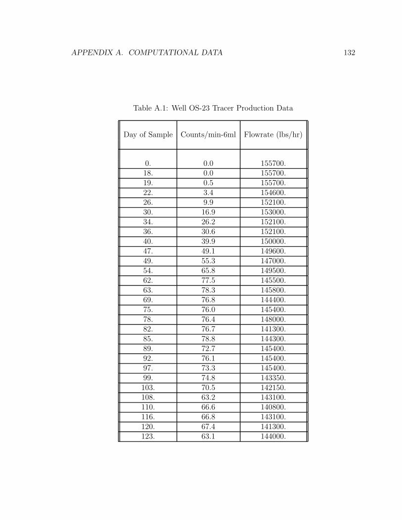
APPENDIX A. COMPUTATIONAL DATA 132
Table A.1: Well OS-23 Tracer Production Data
Day of Sample Counts/min-6ml Flowrate (lbs/hr)
0. 0.0 155700.18. 0.0 155700.19. 0.5 155700.22. 3.4 154600.26. 9.9 152100.30. 16.9 153000.34. 26.2 152100.36. 30.6 152100.40. 39.9 150000.47. 49.1 149600.49. 55.3 147000.54. 65.8 149500.62. 77.5 145500.63. 78.3 145800.69. 76.8 144400.75. 76.0 145400.78. 76.4 148000.82. 76.7 141300.85. 78.8 144300.89. 72.7 145400.92. 76.1 145400.97. 73.3 145400.99. 74.8 143350.103. 70.5 142150.108. 63.2 143100.110. 66.6 140800.116. 66.8 143100.120. 67.4 141300.123. 63.1 144000.

APPENDIX A. COMPUTATIONAL DATA 133
Day of Sample Counts/min-6ml Flowrate (lbs/hr)
125. 61.6 139400.131. 55.6 141750.135. 53.9 142200.138. 98.3 142200.142. 94.8 63100.145. 94.1 62500.149. 88.4 19300.152. 84.7 19800.155. 89.2 147900.160. 54.9 62300.166. 54.3 116800.173. 85.6 39800.180. 53.2 152000.187. 44.8 152000.199. 36.1 140700.201. 44.1 140700.209. 41.0 144900.224. 43.0 144000.229. 42.9 145800.236. 45.2 143100.244. 52.3 60400.252. 54.4 73900.258. 63.7 38900.265. 45.5 144400.272. 34.3 147000.280. 41.9 146934.285. 42.7 149131.

APPENDIX A. COMPUTATIONAL DATA 134
Day of Sample Counts/min-6ml Flowrate (lbs/hr)
292. 48.6 146418.299. 47.1 132655.305. 47.6 137570.314. 44.0 115000.320. 67.3 141000.327. 65.6 101000.335. 43.9 107100.344. 42.9 134300.348. 41.4 132700.352. 38.6 133400.359. 35.0 137100.366. 48.2 139600.376. 40.2 136200.384. 55.5 86800.390. 40.5 144300.397. 37.3 136700.404. 35.2 134700.412. 34.6 131400.418. 33.9 137500.427. 34.1 133800.433. 38.6 133800.439. 39.8 128400.446. 35.9 128100.453. 35.1 128800.460. 38.2 127900.467. 36.2 133300.474. 48.3 131300.

APPENDIX A. COMPUTATIONAL DATA 135
Day of Sample Counts/min-6ml Flowrate (lbs/hr)
481. 38.2 131300.488. 36.6 131300.497. 37.9 131300.502. 35.6 131300.509. 37.8 132900.515. 36.2 133000.524. 35.5 134800.530. 47.7 50400.538. 30.8 137100.546. 34.2 116700.551. 30.5 101900.558. 47.1 101900.565. 41.6 60000.580. 38.2 53000.593. 23.9 125000.607. 31.2 122500.629. 18.2 136800.642. 19.2 104400.657. 18.3 114668.705. 14.8 117126.723. 11.9 117126.734. 11.4 117126.749. 7.0 107700.763. 16.5 107700.782. 14.1 109040.843. 3.3 118220.920. 3.9 135690.

APPENDIX A. COMPUTATIONAL DATA 136
Day of Sample Counts/min-6ml Flowrate (lbs/hr)
1007. 2.0 135690.1036. 6.1 135690.1120. 4.2 135690.1295. 4.4 135690.1331. 7.5 135690.1420. 3.8 135690.

Appendix B
Computer Programs
The following program was used for numerical computations in the semi-analytical
model (Chapter 4).
**************************************************************************
* SOLVES NONLINEAR ODE. *
* *
* JOHN W. HORNBROOK *
* STANFORD UNIVERSITY *
**************************************************************************
*
Parameter (NX = 10000)
Implicit Real*8 (A-H,O-Z)
Real*8 F(NX), X(NX), DXDF(NX), ALPHA(NX), BETA(NX), GAMMA(NX),
* RHS(NX), A(NX), FNEW(NX), ETA(NX), FOLD(NX), DPDRO(NX),
* PRESS(NX), FTAB(NX), PRESSURE(NX), ROV(NX), ROPRESS(NX),
* DENSV(NX), ZPRESS(NX), ZTAB(NX)
Open (Unit=7,File=’INPUT’,Status=’OLD’)
Open (Unit=8,File=’output’,Status=’UNKNOWN’)
Open (Unit=9,File=’fetatable’,Status=’OLD’)
Open (Unit=10,File=’rotable’,Status=’OLD’)
Open (Unit=11,File=’ztable’,Status=’OLD’)
*
137
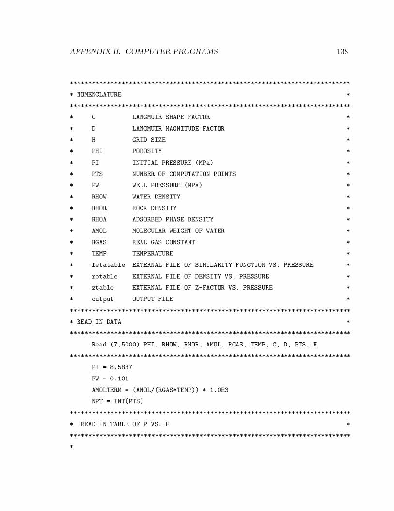
APPENDIX B. COMPUTER PROGRAMS 138
****************************************************************************
* NOMENCLATURE *
****************************************************************************
* C LANGMUIR SHAPE FACTOR *
* D LANGMUIR MAGNITUDE FACTOR *
* H GRID SIZE *
* PHI POROSITY *
* PI INITIAL PRESSURE (MPa) *
* PTS NUMBER OF COMPUTATION POINTS *
* PW WELL PRESSURE (MPa) *
* RHOW WATER DENSITY *
* RHOR ROCK DENSITY *
* RHOA ADSORBED PHASE DENSITY *
* AMOL MOLECULAR WEIGHT OF WATER *
* RGAS REAL GAS CONSTANT *
* TEMP TEMPERATURE *
* fetatable EXTERNAL FILE OF SIMILARITY FUNCTION VS. PRESSURE *
* rotable EXTERNAL FILE OF DENSITY VS. PRESSURE *
* ztable EXTERNAL FILE OF Z-FACTOR VS. PRESSURE *
* output OUTPUT FILE *
****************************************************************************
* READ IN DATA *
****************************************************************************
Read (7,5000) PHI, RHOW, RHOR, AMOL, RGAS, TEMP, C, D, PTS, H
****************************************************************************
PI = 8.5837
PW = 0.101
AMOLTERM = (AMOL/(RGAS*TEMP)) * 1.0E3
NPT = INT(PTS)
****************************************************************************
* READ IN TABLE OF P VS. F *
****************************************************************************
*
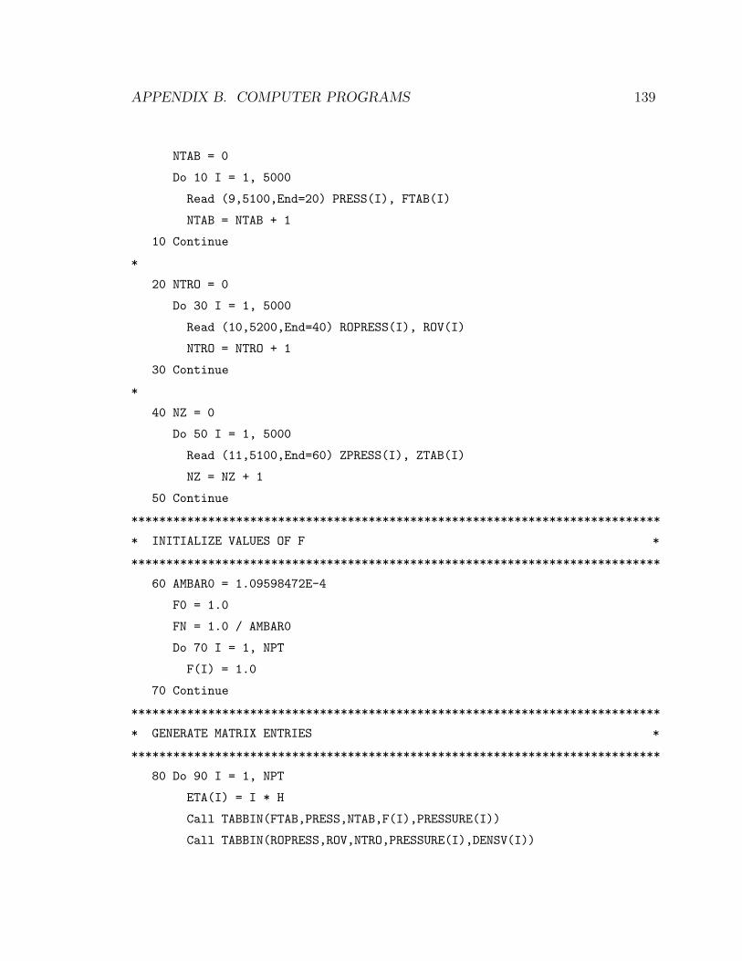
APPENDIX B. COMPUTER PROGRAMS 139
NTAB = 0
Do 10 I = 1, 5000
Read (9,5100,End=20) PRESS(I), FTAB(I)
NTAB = NTAB + 1
10 Continue
*
20 NTRO = 0
Do 30 I = 1, 5000
Read (10,5200,End=40) ROPRESS(I), ROV(I)
NTRO = NTRO + 1
30 Continue
*
40 NZ = 0
Do 50 I = 1, 5000
Read (11,5100,End=60) ZPRESS(I), ZTAB(I)
NZ = NZ + 1
50 Continue
****************************************************************************
* INITIALIZE VALUES OF F *
****************************************************************************
60 AMBAR0 = 1.09598472E-4
F0 = 1.0
FN = 1.0 / AMBAR0
Do 70 I = 1, NPT
F(I) = 1.0
70 Continue
****************************************************************************
* GENERATE MATRIX ENTRIES *
****************************************************************************
80 Do 90 I = 1, NPT
ETA(I) = I * H
Call TABBIN(FTAB,PRESS,NTAB,F(I),PRESSURE(I))
Call TABBIN(ROPRESS,ROV,NTRO,PRESSURE(I),DENSV(I))
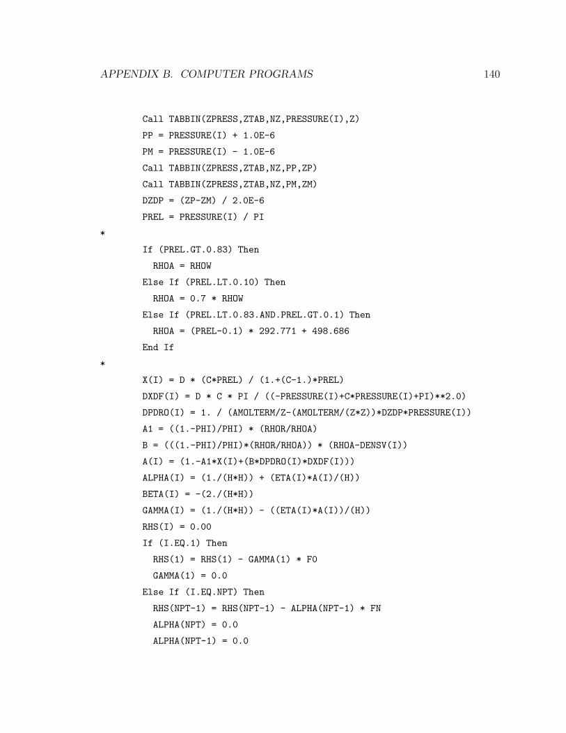
APPENDIX B. COMPUTER PROGRAMS 140
Call TABBIN(ZPRESS,ZTAB,NZ,PRESSURE(I),Z)
PP = PRESSURE(I) + 1.0E-6
PM = PRESSURE(I) - 1.0E-6
Call TABBIN(ZPRESS,ZTAB,NZ,PP,ZP)
Call TABBIN(ZPRESS,ZTAB,NZ,PM,ZM)
DZDP = (ZP-ZM) / 2.0E-6
PREL = PRESSURE(I) / PI
*
If (PREL.GT.0.83) Then
RHOA = RHOW
Else If (PREL.LT.0.10) Then
RHOA = 0.7 * RHOW
Else If (PREL.LT.0.83.AND.PREL.GT.0.1) Then
RHOA = (PREL-0.1) * 292.771 + 498.686
End If
*
X(I) = D * (C*PREL) / (1.+(C-1.)*PREL)
DXDF(I) = D * C * PI / ((-PRESSURE(I)+C*PRESSURE(I)+PI)**2.0)
DPDRO(I) = 1. / (AMOLTERM/Z-(AMOLTERM/(Z*Z))*DZDP*PRESSURE(I))
A1 = ((1.-PHI)/PHI) * (RHOR/RHOA)
B = (((1.-PHI)/PHI)*(RHOR/RHOA)) * (RHOA-DENSV(I))
A(I) = (1.-A1*X(I)+(B*DPDRO(I)*DXDF(I)))
ALPHA(I) = (1./(H*H)) + (ETA(I)*A(I)/(H))
BETA(I) = -(2./(H*H))
GAMMA(I) = (1./(H*H)) - ((ETA(I)*A(I))/(H))
RHS(I) = 0.00
If (I.EQ.1) Then
RHS(1) = RHS(1) - GAMMA(1) * F0
GAMMA(1) = 0.0
Else If (I.EQ.NPT) Then
RHS(NPT-1) = RHS(NPT-1) - ALPHA(NPT-1) * FN
ALPHA(NPT) = 0.0
ALPHA(NPT-1) = 0.0

APPENDIX B. COMPUTER PROGRAMS 141
End If
90 Continue
****************************************************************************
* SOLVE MATRIX PROBLEM *
****************************************************************************
NPTM = NPT - 1
Call THOMAS(BETA,ALPHA,GAMMA,RHS,FNEW,NPTM)
****************************************************************************
* CHECK FOR CONVERGENCE *
****************************************************************************
DIFMAX = ABS(FNEW(1)-F(1))
Do 100 I = 1, NPT
If (FNEW(I).LT.0.0) Then
FNEW(I) = 0.00000
End If
DIF = ABS(FNEW(I)-F(I))
If (DIF.GT.DIFMAX) Then
ID = I
DIFMAX = DIF
End If
100 Continue
DIFTOL = 0.001
If (DIFMAX.GT.DIFTOL) Then
Do 110 I = 1, NPT
If (FNEW(I).LT.0.0) Then
F(I) = 0.000000
Else
F(I) = FNEW(I)
End If
110 Continue
Go To 80
Else
Go To 120

APPENDIX B. COMPUTER PROGRAMS 142
End If
****************************************************************************
* WRITE RESULTS *
****************************************************************************
120 Do 130 I = 1, NPT
FOLD(I) = FNEW(I)
130 Continue
Do 140 I = 1, NPT
Write (8,5300) ETA(I), FNEW(I)
140 Continue
Stop
5000 Format (///5F10.2///5F10.2///F10.2)
5100 Format (E18.4,E18.4)
5200 Format (T12,E13.4,E12.4)
5300 Format (E15.8,5X,E10.4)
End
The following program was used for the simulation of vapor flow in the presence of a
sorbing phase (Chapter 5).
**************************************************************************
* SIMULATES THE FLOW OF VAPOR IN A LINEAR SYSTEM *
* WITH CONSTANT PRESSURE INNER BOUNDARY AND NO *
* FLOW OUTER BOUNDARY. THERMAL EFFECTS ARE INCLUDED. *
* *
* JOHN W. HORNBROOK *
* STANFORD UNIVERSITY *
**************************************************************************
*
Parameter (NX = 300)
Implicit Real*8 (A-H,O-Z)
Real*8 PV(NX), PVO(NX), RHOV(0:NX), VOL(NX), RHOVAV(NX),
* VISCV(NX), VISCVAV(NX), RKRV(NX), AVP(NX), BVP(NX), CVP(NX),
* PSAT(NX), ENINTAN(NX), UV(NX), ENT(NX,NX), B(NX,NX),

APPENDIX B. COMPUTER PROGRAMS 143
* C(NX,NX), RHOVN(NX), AREA(NX), DTVPDPVIP(NX), PSATN(NX),
* DPV(NX), QV(NX), RKRVUP(NX), PVN(NX), VISCVN(NX), RKRVN(NX),
* UVN(NX), DRHOVDPI(NX), DTVPDPVI(NX), DTVMDPVI(NX),
* DTVMDPVIM(NX), DACCNDP(NX), TV(NX), DRODP(NX), DSINKDPI(NX),
* DACCDP(NX), DFLOWDPI(NX), FLOWV(NX), SA(NX), SAN(NX),
* XOLD(NX), XNEW(NX), RHS(NX), RHSACC(NX), SV(NX), SVN(NX),
* DTVDP(NX), DADSDP(NX), RHOA(NX), RHOAN(NX), ENINTV(0:NX),
* TVTEMP(NX), RHSADS(NX), ENINTVN(NX), COND(0:NX), VW(0:NX),
* VV(0:NX), AV(NX), BV(NX), DQDP(NX), DKROMUDP(NX),
* PRESSURE(NX), CV(NX), ENTH(NX), DENSV(NX), VVISC(NX),
* ENTHV(NX), ENTHVN(NX), DXDP(NX), DSRODP(NX), TEMPV(NX),
* TEMPVN(NX), ENINTA(NX),
Common /UNITS/ IT, ID, IP, IH, FT, FD, FP, FH, /UNITC/ NT, ND, NP,
* NH
Common /PARAMS/ TS, DS, PS, Z0, ASS, SSS, RSS, ALPHA(4), BETA(4)
Common /PROPS/ P, AD, GD, HD, UD, SD, CVD, CPD, DPDD, DPDT, DVDT,
* W, CJTT, CJTH
Common /ACONST/ WM, GASCON, TZ, AA, Z, DZ, Y
Open (Unit=7,File=’INPUTADS’,Status=’OLD’)
*
Open (Unit=8,File=’press.out’,Status=’UNKNOWN’)
Open (Unit=9,File=’temp.out’,Status=’UNKNOWN’)
Open (Unit=10,File=’sat.out’,Status=’UNKNOWN’)
****************************************************************************
* NOMENCLATURE *
****************************************************************************
* A SPECIFIES ADSORBED PHASE *
* AREA BLOCK AREA *
* COND THERMAL CONDUCTIVITY *
* DP DELTA PRESSURE *
* DT TIME STEP SIZE *
* DX BLOCK THICKNESS *
* ENINT INTERNAL ENERGY *

APPENDIX B. COMPUTER PROGRAMS 144
* ENTH ENTHALPY *
* N DENOTES NEW TIME ITERATION VALUE *
* O DENOTES OLD TIME ITERATION VALUE *
* P PRESSURE *
* PSAT SATURATION PRESSURE *
* Q MASS FLUX *
* RHO DENSITY *
* RKR RELATIVE PERMEABILITY *
* T TRANSMISSIBILITY *
* TEMP TEMPERATURE *
* U VELOCITY *
* V SPECIFIES VAPOR PHASE *
* VISC VISCOSITY *
* VOL BLOCK VOLUME *
* press.out PRESSURE OUTPUT FILE *
* temp.out TEMPERATURE OUTPUT FILE *
* sat.out SATURATION OUTPUT FILE *
****************************************************************************
* READ IN DATA *
****************************************************************************
Read (7,5000) TMAX, DTMIN, RKRVMAX, SVP, IBCFLG, ALEN, HEIGHT,
* WID, DT, BLK, PERM, CR, PHI, VQ, TEMP, SVI, PVI, AVWO, AVW1,
* AVW2, AVW3, IOPT, IT, ID, IP, IH, DERIVDP, ITMAX, ALANG,
* BLANG, RHOR, ISOCHK, PWF, NB1, NB2, NB3, T1, T2, T3, XB,
* XSLOPE
****************************************************************************
* INITIALIZE BLOCK VALUES *
****************************************************************************
NBLK = INT(BLK)
NBLKP = NBLK + 1
DX = ALEN / BLK
*
Do 10 I = 1, NBLK

APPENDIX B. COMPUTER PROGRAMS 145
SV(I) = SVI
PV(I) = PVI
PVO(I) = PV(I)
PVN(I) = PV(I)
TEMPV(I) = TEMP
TEMPVN(I) = TEMP
10 Continue
*
If (IBCFLG.EQ.1) Then
PV(NBLK) = PWF
PVN(NBLK) = PWF
End If
*
****************************************************************************
* START OUTER LOOP *
****************************************************************************
TIME = 0.0
20 TIME = TIME + DT
ITKOUNT = 0
30 ITKOUNT = ITKOUNT + 1
****************************************************************************
* CALCULATE SATURATION PRESSURES IN EACH BLOCK *
****************************************************************************
Do 40 I = 1, NBLK
40 Continue
****************************************************************************
* CALCULATE ROCK AND FLUID PROPERTIES FOR EACH BLOCK *
****************************************************************************
Do 50 I = 1, NBLK
VOL(I) = DX * WID * HEIGHT
AREA(I) = HEIGHT * WID
* CALCULATE ADSORBATE PROPERTIES
*
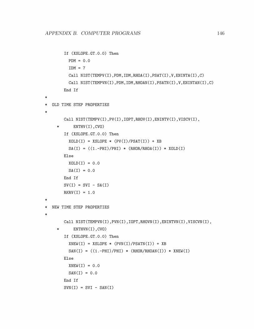
APPENDIX B. COMPUTER PROGRAMS 146
If (XSLOPE.GT.0.0) Then
PDM = 0.0
IDM = 7
Call NIST(TEMPV(I),PDM,IDM,RHOA(I),PSAT(I),V,ENINTA(I),C)
Call NIST(TEMPVN(I),PDM,IDM,RHOAN(I),PSATN(I),V,ENINTAN(I),C)
End If
*
* OLD TIME STEP PROPERTIES
*
Call NIST(TEMPV(I),PV(I),IOPT,RHOV(I),ENINTV(I),VISCV(I),
* ENTHV(I),CVO)
If (XSLOPE.GT.0.0) Then
XOLD(I) = XSLOPE * (PV(I)/PSAT(I)) + XB
SA(I) = ((1.-PHI)/PHI) * (RHOR/RHOA(I)) * XOLD(I)
Else
XOLD(I) = 0.0
SA(I) = 0.0
End If
SV(I) = SVI - SA(I)
RKRV(I) = 1.0
*
* NEW TIME STEP PROPERTIES
*
Call NIST(TEMPVN(I),PVN(I),IOPT,RHOVN(I),ENINTVN(I),VISCVN(I),
* ENTHVN(I),CVO)
If (XSLOPE.GT.0.0) Then
XNEW(I) = XSLOPE * (PVN(I)/PSATN(I)) + XB
SAN(I) = ((1.-PHI)/PHI) * (RHOR/RHOAN(I)) * XNEW(I)
Else
XNEW(I) = 0.0
SAN(I) = 0.0
End If
SVN(I) = SVI - SAN(I)

APPENDIX B. COMPUTER PROGRAMS 147
RKRVN(I) = 1.0
50 Continue
****************************************************************************
* CALCULATE AVERAGE DENSITY AND VISCOSITY AT BLOCK CONNECTION *
****************************************************************************
RHOVAV(1) = 0.0
RHOVAV(NBLKP) = 0.0
VISCVAV(1) = 0.0
VISCVAV(NBLKP) = 0.0
Do 60 I = 2, NBLK
PVNAVG = (PVN(I-1)+PVN(I)) / 2.0
Call NIST(TEMPVN(I),PVNAVG,IOPT,RHOVAV(I),EN,VISCVAV(I),ENT,CV)
60 Continue
****************************************************************************
* CALCULATE TRANSMISSIBILITIES BETWEEN BLOCKS *
****************************************************************************
TV(1) = 0.0
TV(NBLKP) = 0.0
Do 70 I = 2, NBLK
RKRVUP(I) = 1.0
TV(I) = (PERM*RKRVUP(I)*RHOVAV(I)) / (DX*VISCVAV(I))
If (I.EQ.NBLK) Then
TV(NBLK) = (PERM*RKRVUP(NBLK-1)*RHOVN(NBLK-1)) / (DX*
* VISCVN(NBLK-1))
End If
70 Continue
****************************************************************************
* CALCULATE DERIVATIVES IN TV(I+) WITH RESPECT TO PV(I) *
****************************************************************************
DTVPDPVI(1) = 0.0
DTVPDPVI(NBLKP) = 0.0
Do 80 I = 2, NBLK
IM = I - 1

APPENDIX B. COMPUTER PROGRAMS 148
FRONT = PERM * RKRVUP(I) / DX
PVIP = PVN(IM) + DERIVDP
PVIM = PVN(IM) - DERIVDP
Call NIST(TEMPVN(I),PVIM,IOPT,RHOVM,EN,VISCVM,ENT,CV)
Call NIST(TEMPVN(I),PVIP,IOPT,RHOVP,EN,VISCVP,ENT,CV)
TVP = FRONT * (RHOVN(I)+RHOVP) / (VISCVN(I)+VISCVP)
TVM = FRONT * (RHOVN(I)+RHOVM) / (VISCVN(I)+VISCVM)
DTV = TVP - TVM
DPP = 2.0E6 * DERIVDP
DTVPDPVI(I) = DTV / DPP
80 Continue
****************************************************************************
* CALCULATE DERIVATIVES IN TV(I+) WITH RESPECT TO PV(I+1) *
****************************************************************************
DTVPDPVIP(1) = 0.0
DTVPDPVIP(NBLKP) = 0.0
Do 90 I = 2, NBLK
IM = I - 1
FRONT = PERM * RKRVUP(I) / DX
PVIP = PVN(I) + DERIVDP
PVIM = PVN(I) - DERIVDP
Call NIST(TEMPVN(I),PVIM,IOPT,RHOVM,EN,VISCVM,ENT,CV)
Call NIST(TEMPVN(I),PVIP,IOPT,RHOVP,EN,VISCVP,ENT,CV)
TVP = FRONT * (RHOVP+RHOVN(IM)) / (VISCVP+VISCVN(IM))
TVM = FRONT * (RHOVM+RHOVN(IM)) / (VISCVM+VISCVN(IM))
DTV = TVP - TVM
DPP = 2.0E6 * DERIVDP
DTVPDPVIP(I) = DTV / DPP
90 Continue
****************************************************************************
* CALCULATE DERIVATIVES IN TV(I-) WITH RESPECT TO PV(I) *
****************************************************************************
DTVMDPVI(1) = 0.0

APPENDIX B. COMPUTER PROGRAMS 149
DTVMDPVI(NBLKP) = 0.0
Do 100 I = 2, NBLK
IM = I - 1
FRONT = PERM * RKRVUP(I) / DX
PVIP = PVN(I) + DERIVDP
PVIM = PVN(I) - DERIVDP
Call NIST(TEMPVN(I),PVIM,IOPT,RHOVM,EN,VISCVM,ENT,CV)
Call NIST(TEMPVN(I),PVIP,IOPT,RHOVP,EN,VISCVP,ENT,CV)
TVP = FRONT * (RHOVN(IM)+RHOVP) / (VISCVN(IM)+VISCVP)
TVM = FRONT * (RHOVN(IM)+RHOVM) / (VISCVN(IM)+VISCVM)
DTV = TVP - TVM
DPP = 2.0E6 * DERIVDP
DTVMDPVI(I) = DTV / DPP
100 Continue
****************************************************************************
* CALCULATE DERIVATIVES IN TV(I-) WITH RESPECT TO PV(I-1) *
****************************************************************************
DTVMDPVIM(1) = 0.0
DTVMDPVIM(NBLKP) = 0.0
Do 110 I = 2, NBLK
IM = I - 1
FRONT = PERM * RKRVUP(I) / DX
PVIP = PVN(IM) + DERIVDP
PVIM = PVN(IM) - DERIVDP
Call NIST(TEMPVN(I),PVIM,IOPT,RHOVM,EN,VISCVM,ENT,CV)
Call NIST(TEMPVN(I),PVIP,IOPT,RHOVP,EN,VISCVP,ENT,CV)
TVP = FRONT * (RHOVP+RHOVN(I)) / (VISCVP+VISCVN(I))
TVM = FRONT * (RHOVM+RHOVN(I)) / (VISCVM+VISCVN(I))
DTV = TVP - TVM
DPP = 2.0E6 * DERIVDP
DTVMDPVIM(I) = DTV / DPP
110 Continue
****************************************************************************

APPENDIX B. COMPUTER PROGRAMS 150
* CALCULATE DERIVATIVES OF DENSITY AND X IN BLOCK I W.R.T. PV(I) *
****************************************************************************
Do 120 I = 1, NBLK
PVP = PVN(I) + DERIVDP
PVM = PVN(I) - DERIVDP
Call NIST(TEMPVN(I),PVM,IOPT,RHOVNM,EN,VISCVM,ENT,CV)
Call NIST(TEMPVN(I),PVP,IOPT,RHOVNP,EN,VISCVP,ENT,CV)
DRO = RHOVNP - RHOVNM
DPP = 2.0E6 * DERIVDP
DRODP(I) = DRO / DPP
*
If (XSLOPE.GT.0.0) Then
XUP = XSLOPE * (PVP/PSAT(I)) + XB
XDWN = XSLOPE * (PVM/PSAT(I)) + XB
DELTAX = XUP - XDWN
DXDP(I) = DELTAX / DPP
Else
XUP = 0.0
XDWN = 0.0
DELTAX = 0.0
DXDP(I) = 0.0
End If
*
If (XSLOPE.GT.0.0) Then
SAUP = ((1.-PHI)/PHI) * (RHOR/RHOA(I)) * XUP
SADN = ((1.-PHI)/PHI) * (RHOR/RHOA(I)) * XDWN
SVUP = SVI - SAUP
SVDN = SVI - SADN
DSRO = SVUP * RHOVNP - SVDN * RHOVNM
DSRODP(I) = DSRO / DPP
Else
SAUP = 0.0
SADN = 0.0

APPENDIX B. COMPUTER PROGRAMS 151
SVUP = 0.0
SVDN = 0.0
DSRO = 1.0 * (RHOVNP-RHOVNM)
DSRODP(I) = DSRO / DPP
End If
120 Continue
****************************************************************************
* CONSTRUCT AV(I) TERMS *
****************************************************************************
DFLOWDPI(1) = DTVPDPVI(2) * (PVN(2)-PVN(1)) - TV(2)
DFLOWDPI(NBLK) = 0.0
Do 130 I = 2, NBLK - 1
IUP = I + 1
IM = I - 1
*
* FLOW TERM
*
DFLOWDPI(I) = DTVPDPVI(IUP) * (PVN(IUP)-PVN(I)) - DTVMDPVI(I) *
* (PVN(I)-PVN(IM)) - TV(IUP) - TV(I)
130 Continue
*
* ACCUMULATION TERM AND ADSORPTION TERMS
*
Do 140 I = 1, NBLK
DACCDP(I) = (PHI*DX/DT) * (DSRODP(I))
DADSDP(I) = ((1.-PHI)*RHOR*DX/DT) * (DXDP(I))
140 Continue
*
* AV(I)
*
Do 150 I = 1, NBLK
AV(I) = DFLOWDPI(I) - DACCDP(I) - DADSDP(I)
150 Continue
APPENDIX B. COMPUTER PROGRAMS 152
****************************************************************************
* CONSTRUCT BV(I) TERMS *
****************************************************************************
BV(NBLK) = 0.0
BV(NBLK-1) = 0.0
Do 160 I = 1, NBLK - 2
IUP = I + 1
BV(I) = DTVPDPVIP(IUP) * (PVN(IUP)-PVN(I)) + TV(IUP)
160 Continue
****************************************************************************
* CONSTRUCT CV(I) TERMS *
****************************************************************************
CV(1) = 0.0
Do 170 I = 2, NBLK - 1
IM = I - 1
CV(I) = (-1.) * (DTVMDPVIM(I)*(PVN(I)-PVN(IM))) + TV(I)
170 Continue
****************************************************************************
* CONSTRUCT THE RIGHT HAND SIDE VECTOR *
****************************************************************************
*
* FLOW TERM
*
FLOWV(1) = TV(2) * 1.0E6 * (PVN(2)-PVN(1))
FLOWV(NBLK) = 0.0
Do 180 I = 2, NBLK - 1
IUP = I + 1
IM = I - 1
FLOWV(I) = TV(IUP) * 1.0E6 * (PVN(IUP)-PVN(I)) - TV(I) * 1.0E6 *
* (PVN(I)-PVN(IM))
180 Continue
*
* ACCUMULATION TERM AND ADSORPTION TERM

APPENDIX B. COMPUTER PROGRAMS 153
*
Do 190 I = 1, NBLK - 1
RHSACC(I) = (DX/DT) * PHI * (SVN(I)*RHOVN(I)-SV(I)*RHOV(I))
RHSADS(I) = (DX/DT) * PHI * (SAN(I)*RHOAN(I)-SA(I)*RHOA(I))
190 Continue
*
Do 200 I = 1, NBLK - 1
RHS(I) = FLOWV(I) - RHSACC(I) - RHSADS(I)
RHS(I) = -RHS(I)
200 Continue
****************************************************************************
* SOLVE MATRIX PROBLEM *
****************************************************************************
NBMINUS = NBLK - 1
Call THOMAS(AV,BV,CV,RHS,DPV,NBMINUS)
****************************************************************************
* CALCULATE VELOCITY IN EACH BLOCK AND MASSS FLOW RATE FROM LAST BLOCK *
****************************************************************************
*
QV(NBLK-1) = (PERM*RKRVUP(NBLK-1)*RHOVN(NBLK-1)*AREA(NBLK-1)) * ((
* PVN(NBLK-1)-PVN(NBLK))*1.0E6) / ((DX/2.)*VISCVN(NBLK-1))
Do 210 I = 1, NBLK - 1
VVTEMP = (PERM*RKRVUP(NBLK-1)/(VISCVN(NBLK-1)*DX)) * (PVN(I)-
* PVN(I+1)) * 1.0E6
VV(I) = ABS(VVTEMP)
210 Continue
****************************************************************************
* COMPUTE HEAT BALANCE *
****************************************************************************
If (ISOCHK.EQ.1) Then
Do 220 I = 1, NBLK
*
SV(0) = 0.0
APPENDIX B. COMPUTER PROGRAMS 154
RHOV(0) = 0.0
ENINTV(0) = 0.0
VV(0) = 0.0
*
SV(NBLK+1) = 0.0
RHOV(NBLK+1) = 0.0
ENINTV(NBLK+1) = 0.0
VV(NBLK+1) = 0.0
*
TEMPV(NBLK+2) = 0.0
TEMPV(NBLK+1) = 0.0
TEMPV(0) = 0.0
TEMPV(-1) = 0.0
*
COND(0) = 0.0
COND(NBLK+1) = 0.0
IUP = I + 1
IPP = I + 2
IM = I - 1
IMM = I - 2
Call HEATBV(DX,DT,PHI,SV(I),SVN(I),RHOV(I),RHOVN(I),
* ENINTV(I),ENINTVN(I),RHOR,ENINTR,ENINTRN,PERM,RKRV(I),
* MDOT,VV(I),SV(IP),RHOV(IUP),ENINTV(IUP),VV(IUP),SV(IM),
* RHOV(IM),ENINTV(IM),VV(IM),PV(I),TEMPV(I),TEMPV(IPP),
* TEMPV(IMM),VISCV(I),COND(IM),COND(IUP),TRN,VOL(I),QV(I),
* ENTHVN(I),SA(I),SAN(I),RHOA(I),RHOAN(I),ENINTA(I),
* ENINTAN(I))
TEMPVN(I) = TRN
220 Continue
End If
****************************************************************************
* CHECK FOR MAXIMUM DELTA PV *
****************************************************************************

APPENDIX B. COMPUTER PROGRAMS 155
DPVMAX = ABS(DPV(1))
Do 230 I = 1, NBLK
If (ABS(DPV(I)).GT.DPVMAX) Then
DPVMAX = ABS(DPV(I))
End If
230 Continue
****************************************************************************
* CHECK FOR MAXIMUM RIGHT HAND SIDE *
****************************************************************************
RHSMAX = ABS(RHS(1))
Do 240 I = 1, NBLK
If (ABS(RHS(I)).GT.RHSMAX) Then
RHSMAX = ABS(RHS(I))
End If
240 Continue
****************************************************************************
* CHECK TO SEE THAT DPV AND RHS VALUES ARE WITHIN TOLERANCES *
****************************************************************************
RHSTOL = 1.0E-8
DPVTOL = 1.000
If (RHSMAX.LE.RHSTOL.AND.DPVMAX.LE.DPVTOL) Then
Do 250 I = 1, NBLK
PVN(I) = PVN(I) + DPV(I) * 1.0E-6
PV(I) = PVN(I)
TEMPV(I) = TEMPVN(I)
250 Continue
****************************************************************************
* WRITE OUTPUT *
****************************************************************************
*
* HISTORIES
*
Write (8,5100) TIME, PVN(1)

APPENDIX B. COMPUTER PROGRAMS 156
Write (9,5100) TIME, TEMPVN(2)
Write (10,5100) TIME, SAN(3)
****************************************************************************
If (TIME.GE.TMAX) Then
Go To 270
Else
Go To 20
End If
Else
Do 260 I = 1, NBLK
PVN(I) = PVN(I) + DPV(I) * 1.0E-6
260 Continue
If (ITKOUNT.GE.ITMAX) Then
Print *, ’MAXIMUM ITERATION CONSTRAINT EXCEEDED’
Else
Go To 30
End If
End If
270 Stop
5000 Format (///4F10.2,I10///3F10.2,2E15.2///2E10.2,3F10.2///5F10.2///
* F10.2,4I10///I10,F10.2,I10,F10.2,F10.2///F10.2,I10,F10.2,2I10
* ///I10,4F10.2,///F10.2)
5100 Format (E15.8,5X,E20.9)
5200 Format (I10,5X,F15.4)
End
The following subroutine was used to calculate the heat balance for the flow of vapor
in the presence of a sorbing phase.
********************************************************************
* *
* CALCULATES HEAT BALANCE FOR VAPOR FLOW *
* *
* JOHN W. HORNBROOK *
APPENDIX B. COMPUTER PROGRAMS 157
* STANFORD UNIVERSITY
********************************************************************
Subroutine HEATBV(DX,DT,PHI,SV,SVN,RHOV,RHOVN,ENINTV,ENINTVN,RHOR,
* ENINTR,ENINTRN,PERM,RKV,MDOT,VV,SVP,RHOVP,ENINTVP,VVP,SVM,
* RHOVM,ENINTVM,VVM,PV,TEMP,TEMPP,TEMPM,TEMPNI,TEMPNUP,TEMPNDN,
* VISCV,CONDM,CONDP,TRN,VOL,Q,ENTH,SA,SAN,RHOA,RHOAN,ENINTA,
* ENINTAN)
Implicit Real*8 (A-H,O-Z)
Real*8 NINE
CPR = 1.017
CONDR = 2.5
********************************************************************
* NOMENCLATURE *
********************************************************************
* CONDR ROCK CONDUCTIVITY *
* CPR ROCK SPECIFIC HEAT *
* DT TIME STEP SIZE *
* DX BLOCK THICKNESS *
* ENINTA ADSORBATE INTERNAL ENERGY AT OLD TIME STEP *
* ENINTAN ADSORBATE INTERNAL ENERGY AT NEW TIME STEP *
* ENINTVM VAPOR INTERNAL ENERGY IN DOWNSTREAM BLOCK *
* ENINTVP VAPOR INTERNAL ENERGY IN UPSTREAM BLOCK *
* ENTH ENTHALPY OF PROUCED FLUID *
* PERM PERMEABILITY *
* PHI POROSITY *
* Q MASS FLOW RATE OUT OF PRODUCTION BLOCK *
* RHOR ROCK DENSITY *
* RHOV VAPOR DENSITY AT OLD TIME STEP *
* RHOVM VAPOR DENSITY AT DOWNSTREAM BLOCK *
* RHOVP VAPOR DENSITY AT UPSTREAM BLOCK *
* SA ADSORBED PHASE SATURATION AT OLD TIME STEP *
* SAN ADSORBED PHASE SATURATION AT NEW TIME STEP *
* SVM VAPOR PHASE SATURATION AT DOWNSTREAM BLOCK *

APPENDIX B. COMPUTER PROGRAMS 158
* SVP VAPOR PHASE SATURATION AT UPSTREAM BLOCK *
* TEMP TEMPERATURE AT OLD TIME STEP *
* TRN TEMPERATURE AT NEW TIME STEP *
* VOL BLOCK VOLUME *
* VVP VAPOR VELOCITY IN UPSTREAM BLOCK *
* VVM VAPOR VELOCITY IN DOWNSTREAM BLOCK *
********************************************************************
*
ONE = (RHOR/DT) * (((1.-PHI)*CPR*TRN)-((1.-PHI)*CPR*TEMP))
*
THREE = (1./DT) * ((SVN*PHI*RHOVN*ENINTVN)-(SV*PHI*RHOV*ENINTV))
*
FOUR = (1./DT) * ((SAN*PHI*RHOAN*ENINTAN)-(SA*PHI*RHOA*ENINTA))
*
FIVE = (CONDR/DX) * (TEMPNUP-2.*TEMPNI+TEMPNDN)
*
SIX = (1./(2.*DX)) * ((PHI*SVP*RHOVP*ENINTVP*VVP)-(PHI*SVM*RHOVM*
* ENINTVM*VVM))
*
NINE = 1.0E3 * (PV/(2.*DX)) * ((PHI*SVP*VVP)-(PHI*SVM*VVM))
*
ELEVEN = 1.0E-3 * ((SV**2.)*(PHI**2.)*VISCV*(VV**2.)) / (PERM*RKV)
*
FLUX = Q * (ENTH) / VOL
*
RHS = (-THREE-FOUR+FIVE-SIX-NINE+ELEVEN-FLUX)
RHSMOD1 = (DT/RHOR) * RHS
RHSMOD2 = RHSMOD1 + ((1.-PHI)*CPR*TEMP)
TRN = RHSMOD2 / ((1.-PHI)*CPR)
Return
End

APPENDIX B. COMPUTER PROGRAMS 159
A number of subroutines are not included in this text but can be found elsewhere.
Subroutine NIST is available from the National Institute of Standards and Technology
[26] and subroutines THOMAS and TABBIN which solve a tridiagonal matrix and
perform linear interpolation, respectively, are available from Aziz and Settari [6].