THE ESTIMATION OF COMPONENTS OF HOUSEHOLD

INCOMES AND EXPENDITURES: A Methodological Guide based on the Ghana Living Standards Survey,

1991/1992 and 1998/1999

GHANA STATISTICAL SERVICE, ACCRA OCTOBER 2000

ii

Copyright © 2000 Ghana Statistical Service

Ghana Statistical Service P O Box GP 1098

Accra

iii

THE ESTIMATION OF COMPONENTS OF HOUSEHOLD INCOMES AND EXPENDITURES:

A Methodological Guide based on the Ghana Living Standards Survey, 1991/1992 and 1998/1999

Harold Coulombe Andrew McKay

October 2000 Acknowledgements: This work has also greatly benefited from earlier contributions from Jeff Round from the University of Warwick. The authors are grateful to the Data Processing staff at the Statistical Service for their great hospitality and continuous support; and to Gabrielle Cournoyer for her excellent research assistance. This work has been undertaken with financial support by the Ghana Statistical Service, through the World Bank, and also partly by the European Union.

iv

PREFACE This report represents a description of the methodology used in the estimation of the components of the household income and expenditure in the fourth round of the Ghana Living Standards Surveys (GLSS 4). The main purpose of this report is to assist users of the GLSS 4 results to understand the way the various household income and expenditure components were calculated. It is therefore most useful when read in conjunction with the main report. The GLSS 4 is the latest of four nationwide living standards surveys conducted by the Ghana Statistical Service on a wide range of topics including demographic characteristics of the population, education, health employment and time use, migration, housing conditions, household agriculture and non-farm businesses. The main objective of the GLSS is to provide benchmark data on the living standards of the population as well as monitor and evaluate progress made by planners and policy makers in raising and sustaining those standards. The GLSS 4, however, focused on labour force. This report has been prepared by Harold Coulombe and Andrew D. Mckay with technical support from the World Bank and the Ghana Statistical Service. We also wish to acknowledge with thanks the support provided by the European Union.

DR. K. A. TWUM-BAAH (AG. GOVERNMENT STATISTICIAN AND PROJECT TECHNICAL DIRECTOR)

v

CONTENTS

1. Introduction ................................................................................................................................. 1

2. Household Income and Expenditure Concepts........................................................................... 2

3. Components of Income and Expenditure.................................................................................... 4

4. Calculation of Income and Expenditure Components in Practice.............................................. 8

5. Statistical Summary of the GLSS 1 and GLSS 2 Estimates..................................................... 12

Appendix 1. Sources and Methods for the Calculation of Income and Expenditure Aggregates .. 19

Appendix 2. Estimation of Imputed Rental Values for Housing ................................................. 29

Appendix 3. Description of Variables .......................................................................................... 32

Appendix 4. Definition of Aggregates and Subaggregates .......................................................... 39

Appendix 5. Aide-Mémoire to Programs and Data Sets .............................................................. 44

1

I. INTRODUCTION

The aim of the present study is to estimate components of income and expenditure at the household level based on the results of the third and fourth round of the Ghana Living Standards Survey, conducted by the Ghana Statistical Service in 1991/1992 and 1998/1999 respectively. This is a multidimensional household survey collecting information on a wide variety of household and individual level variables, including detailed information on incomes and expenditures. This document seeks to explain the construction of a coherent and consistent set of estimates of household incomes and expenditures based on the information collected by these surveys. Estimates of household income and expenditure are of interest for a wide variety of statistical and analytical purposes. One of the most obvious may be for the estimation of household welfare and of poverty; however, given the wide variety of purposes for which information on components of household income and expenditure may be required, the aim here has been to construct a detailed and flexible hierarchy of estimates at different levels of aggregation. While the focus of this document is primarily on relatively aggregate household income and expenditure components, in fact a whole series of more disaggregated estimates have also been produced in the calculation process. These more disaggregated components are likely to be of interest in their own right for many purposes; further, their availability permits the construction of alternative aggregate components as users see fit. This document should be read in conjunction with the third and fourth round GLSS household questionnaires, to which it often refers; the same overall questionnaire structure was used for both surveys although some small differences can be found in few sections of the questionnaire. The text of the document discusses in general terms the conceptual issues underlying the estimation of household income and expenditure components in a household accounting framework (Section 2), sets out a description of the aggregate level components which have been estimated (Section 3), explains the calculation procedure which has been adopted (Section 4), and presents a statistical summary of aspects of the estimation process for the GLSS 3 and 4 surveys (Section 5). More technical details are provided in the five appendices, which provide detailed information on the contents of the aggregate level components (Appendix 1), on the estimation of imputed housing rents (Appendix 2), descriptions of the subaggregate level variables (Appendix 3), definitions of the subaggregates and aggregates (Appendix 4), and a concise description of the SAS computer programs used to carry out the calculation procedures as set out in Section 4 (Appendix 5). It should be noted that this document, and the programs which accompany it, relate only to the last two rounds of results of the Ghana Living Standards Survey. The questionnaires used for the first two rounds of the GLSS differ a lot from the ones used here; however, the appropriate procedures and the general structure of the programs required are essentially the same. A document similar to the present one explaining the GLSS 1 and 2 aggregates can be obtained from the Ghana Statistical Service.

2

2. HOUSEHOLD INCOME AND EXPENDITURE CONCEPTS1

Income and expenditure aggregates at the household level are most conveniently considered within the context of a broader system of accounts that focus on the household as a producer, consumer and accumulator of assets and liabilities. In such a framework, it is easier to understand the inevitable boundary problems inherent in defining what should be included or excluded in the different components of household incomes and expenditures. These problems, which arise at both the conceptual and the practical level, have been tackled in most systems of national accounts and, in particular, in the United Nations System of National Accounts (SNA), where the issues involved for the household sector were again reconsidered in the 1993 revision and continue to be considered subsequently. Similar issues arise in the present exercise, even though the focus here is on individual households rather than on the household sector in aggregate (as in the national accounts). In fact, the household-level estimates for Ghana to which this note refers are derived using more or less conventional national accounting definitions of what constitutes household incomes and expenditures. However, the unusually wide scope of the Ghana Living Standards Survey is designed to provide much more information on the economic activities of households than is often the case in household surveys, so the estimates derived are more readily obtainable from this one source. This particularly applies to the information relating to the household as a producing unit which, hitherto, has been a relatively neglected area in such surveys even though many households in developing countries are engaged directly in production activities. From the standpoint of the household accounts, and especially the estimated components reported on in this note, this implies the need to explicitly introduce a household production account. This then impinges on the household income and expenditure account in that its balance, net revenue from household production activities, constitutes a component of household income. In this context it is helpful to maintain a distinction between agricultural and non-agricultural household production activity; and this is reflected in the choice of income aggregates. Apart from transfer income referred to shortly, household members typically derive their income in two ways. First, they sell their labour services to other production units in the economy and receive wages or salaries in return, either in cash or in kind. Secondly, they may receive income from production assets which they own. In practice a major source of this is rent on the ownership of dwellings; either actual rent, or in the case of owner occupied dwellings, imputed rent. Income from own account production activities is intermediate between these two in that it represents a return to both labour and capital services provided by the household. In practice it usually difficult to calculate the return to each of these factors individually, but in any case the distinction is unimportant for the present exercise. Non factor income can arise as transfers between households or as a receipt or transfer from other institutions such as government (e.g. educational scholarships). Such income receipts may be highly transient and it may be difficult to distinguish them from capital transfers at the margin (e.g. gifts received and dowry). This is a good illustration of why it might be valuable to compile both current and capital accounts for households. Any transaction or transfer that may be excluded from one account would be automatically included in the other and hence any

1 The conceptual issues raised in the construction of estimates of components of household incomes and expenditures are discussed in more detail in M. Johnson, A.D. McKay and J.I. Round, Income and Expenditure in a System of Household Accounts: Concepts and Definitions, SDA Working Paper No. 10, World Bank, Washington D.C., September 1990.

3

arbitrariness in determining the boundary for the income (and expenditure) aggregates (within the strict context of the current account) would, at least in part, be offset by the inclusion of the capital account. Each of the current and capital accounts should balance with household savings constituting the derived or balancing item that is common to both. Consequently, the combined current and capital accounts should balance overall and household savings would net out through consolidation. For present purposes only current account aggregates have been derived because it would be difficult or impossible in practice to estimate a complete set of capital accounts from the information provided by the survey2. On the expenditure side of the household (current) accounts, in addition to recorded cash expenditures (on food, services, housing, etc.) the survey provides information on household consumption of home produced goods (and services). Clearly, this is especially important in respect of subsistence agriculture but it is conceptually no different for domestic consumption of the output of non-farm production activities. Likewise, non cash incomes in kind (e.g. housing subsidies) should be included as an imputed expenditure. These expenditures also appear as an element of income, as indicated earlier. The need to make these imputations is generally accepted in principle, although in many cases it is difficult to obtain estimates in practice and they are frequently excluded from many countries' national accounts estimates. In the present case, however, the GLSS survey results offer some scope for imputing values of such incomes and expenditures, and these estimates are included in the household level aggregates for Ghana. A final area of conceptual development where a departure from existing conventions may arise concerns the treatment of consumer durables. Viewing the household as a consumer, national accounting conventions treat all purchases of durable goods as a current expenditure. Houses would be a capital purchase, however, since they are regarded as generating housing services which, for owner occupiers, would constitute both an income and an expenditure stream. A legitimate question can be posited as to whether other consumer durables (cooking and heating appliances, etc.) may be treated similarly and, if so, what might be the most appropriate method of imputing consumption flows or 'use values'. The estimates for Ghana include some estimates of 'use values' for durable goods. Unfortunately for reasons explained later, these use values have had to be based on assumed depreciation rates and are thus not entirely satisfactory. This is an area where further research and statistical enquiry may be necessary, including changes in questionnaire design, before there can be an improvement in methods of estimation.

2 For example, no information is available on stockbuilding by households, which may be especially important for households engaged in own-account production activities.

4

3. COMPONENTS OF INCOME AND EXPENDITURE Detailed estimates of income and expenditure components at the household level may be sought at many levels of disaggregation. For present purposes it has proved convenient to assemble estimates of six categories of income and six categories of expenditure; these are referred to as aggregates and are selected in such a way as to combine elements which are logically similar in nature in ways which will be potentially useful for analysis3. In addition, estimates are provided of the detailed components which make up these aggregates, referred to as subaggregates; these will also be important for many analytic purposes for which more detailed information is required. These subaggregates, although they may exist at different levels of aggregation, bear a much closer relationship to the income and expenditure variables actually collected in the questionnaire. This section focuses primarily on the aggregates, describing the content and scope of the estimates. Detailed sources and methods for each of these categories are described in Appendix 1. The subaggregate variables are referred to only in general terms; more detailed information on the subaggregates is provided in Appendix 3 (which provides a listing) and Appendix 4 (which defines the subaggregates and explains their correspondence with the aggregates). INCOME CATEGORIES (1) Income from employment In many households there may be more than one individual who is an active member of the labour force. Moreover, such individuals may undertake more than one economic activity during any year, any week, or indeed, at any period of time. This income category relates solely to employee compensation (either in cash or imputed in kind) with annual estimates of such income being computed for each individual household member. It may well be that an individual is not only an employee but also works in an own household enterprise or on own account. These latter incomes are included elsewhere (in income categories (2) or (3)). This category is strictly confined to employee compensation whether the employment is in a corporate enterprise or an unincorporated family run activity operated by a member of some other household, and whether or not this is the principal or secondary occupation of the individual. (2) Household agricultural income Household members engaged in own account agricultural activities receive income derived either explicitly from the sale of cash crops or livestock products, or implicitly from the consumption of homegrown agricultural produce. To obtain this measure of income two approaches are possible. First, an estimate of the total input costs of such agricultural activity (seeds, fertilizer, feed etc.), inclusive of wages paid to non household members and an allowance for the depreciation of capital assets, may be deducted from an estimate of the value of gross output. Secondly, estimates of self employment income from agricultural activity may be obtained directly. The two estimates are not necessarily equally reliable; while both have been estimated here, the former is considered preferable in this case. Either way, the incomes 3 It should be noted that there is an important revision in the names and composition of these aggregates, compared with those used in the earlier exercise based on GLSS 3.

5

generated represent a combination of returns to both labour and productive capital owned and operated by household members. (3) Non-farm self employment income This constitutes all income from own account activities other than those that are agriculture based. The principles for deriving the estimates are the same, however. Estimates of total household income can be obtained by estimating the value of gross output (inclusive of an imputed value of any home consumption or of commodities transacted in kind) and subtracting the current cost of all inputs other than factor services provided by the household and its members, including an allowance for the depreciation of capital assets owned and employed by them. The survey, however, permits two other alternative estimates to be constructed, one based on direct information on self employment income and the other on a direct question about profits; in fact, in this case these latter estimates are judged much preferable to the first estimate which, more often than not, gives negative income estimates. The direct question on profits is probably the best estimate. As with agricultural income (category (2)) this income category will constitute a return to both labour and capital supplied by the household. However, households may operate more than one unincorporated business enterprise and the GLSS questionnaire allows income estimates to be made for up to three such enterprises. These are totalled for each household. (4) Income from rent A further element of factor income received by households relates to rent. This includes actual income received from leasing land, equipment, buildings or dwellings. In addition, imputed rent has to be included especially in regard to owner occupied dwellings, with a corresponding imputed expenditure on dwelling services (see expenditure category (8)). These estimates of imputed rents were based on the predictions of hedonic equations, which related the actual or potential rental value of dwellings to their characteristics and amenities. (5) Income from remittances This income category relates to current transfers received by households from other households. In addition to the conventional concept of remittances, that is payments in the form of cash or goods, this category also includes an imputation corresponding to the provision to a household of rent-free or subsidised accommodation by another household (including cases in which the dwelling is occupied by squatters). The latter item represents a current transfer paid in kind and a value is imputed to such transfers based on the hedonic equation referred to above. In each case it is assumed that these remittances in cash or kind are not due to be repaid. If remittances are due to be repaid then they should not be included here but should be included instead in the capital account. While the validity of this assumption cannot be checked using the survey results, it seems a reasonable assumption given that most remittances are made as part of the “extended family system” within which there is generally no economic obligation for repayment. (6) Other Income

6

All other incomes received are aggregated into this final component. It includes a mixture of transfers and factor incomes of various kinds from outside the household sector, covering elements such as social security, pension receipts, educational scholarships, together with dividends on investments, interest on savings and certain windfall gains. In this instance, the majority of the items recorded in the GLSS questionnaire as 'miscellaneous income' are included in this category although it may be arguable in some cases whether they might be more appropriately treated as a capital receipt rather than as income. EXPENDITURE CATEGORIES (7) Food expenditure (actual) Expenditure on food by households is a relatively straightforward category of household expenditure. Although individual commodity level estimates are available from the questionnaire, and are included among the subaggregates, this component consists of a simple aggregation of them over all items. It should be noted that this estimate is based on several visits. (8) Housing expenditure (actual and imputed) This component includes actual expenditure on rent, an imputed rental value for owner-occupied dwellings, an imputation of rent for those households who receive subsidised or rent-free housing from employers, relatives or others, and an imputation of rent for those who neither own nor rent their dwellings (such as squatters). Each of these three types of imputations is made on the basis of the hedonic equation previously referred to, except in the case of housing subsidies provided by employers for which a valuation is available separately. In the case of each of these imputations, exactly analogous elements are included among the income components. (9) Other expenditure (actual) This category of household expenditure on goods and services contains an aggregate of all consumption expenditure made in monetary form, except for that on food and housing (already included in components (7) and (8) above respectively). It includes such elements as clothing and footwear, household management, personal care products, energy and fuels, health and education, other services, and infrequent expenditures (eg. jewellery). (10) Food expenditure (imputed) This component covers two types of imputation, firstly the domestic consumption of own output by households engaged in agricultural production, and secondly the value of any wage income received by household members in the form of food. In both cases the valuations for these imputations are supplied by respondents, in principle using market prices. Both of these imputations are also included among the income aggregates (categories (2) and (1) respectively). (11) Other expenditure (imputed) This is an analogue of category (10) for non food items, including domestic consumption of the

7

output of household non-farm enterprises, and wage payment in kind received in any form other than food or housing (the latter being included in category (8) above). Again market price valuations of these elements are supplied by respondents, and corresponding imputations are included among the income aggregates. In addition, however, it includes an estimate of the 'use value' of durable goods (as opposed to expenditure on durable goods per se). In line with increasing trends in current practice, purchases of durable goods are considered to represent capital expenditures with 'use values' or consumption flows being estimated here essentially as the depreciation of these capital assets. As a consequence of this, 'use values' appear as a current expenditure although incomes of households are unaffected. (12) Expenditure on remittances An item consistent with the treatment of remittances received (category (5)) is the transfer payment of remittances to other households. These are estimated directly from survey responses to questions concerning payments in money and in kind. Unfortunately, it is not possible to estimate the counterpart of the second type of transfer included in the income category, that is the provision by households of rent-free or subsidised housing to other households. However, the same problem arises as with its income counterpart in that current and capital remittances cannot satisfactorily be distinguished.

8

4. CALCULATION OF INCOME AND EXPENDITURE COMPONENTS IN PRACTICE The previous section has described the income and expenditure components at the aggregate level which are to be estimated based on the third and fourth rounds of the GLSS surveys. However, the calculation of these components is anything but trivial. In general, the income and expenditure variables are collected at a highly disaggregated level, partially in order to (hopefully) facilitate more accurate estimates of aggregate variables and partially because this disaggregated information is of interest in its own right. There is thus the need for a process of aggregation. Prior to this, however, three other issues must be taken into account4. Firstly, the variables collected in the questionnaire relate to a variety of different reference periods, so that there is a need for a process of standardisation, expressing all variables on a consistent annual basis but taking due account of intra-year variations (eg. due to seasonality) as much as this is practically possible. Secondly, outliers have to be identified and re-estimated across the sample. Thirdly, missing values of the variables should be re-estimated where appropriate. This section describes the procedures used for these four aspects of standardisation, outliers, missing values and aggregation; the programs (written using the software SAS) used to conduct these various stages are briefly described in Appendix 5. This calculation procedure may be represented by the following four stages, each of which corresponds to a series of programs, and which should logically be carried out in this order. (i) Standardisation As noted above, the income and expenditure variables collected by the questionnaire generally relate to a range of different reference periods; for example, earnings may be quoted per week, per month, per year etc. In this stage of the calculation procedure all income and expenditure variables are expressed on a consistent annual basis. For many such variables this process is trivial because they are already quoted by respondents on an annual basis. This applies to many of the less regular and less frequent sources of income (such as educational scholarships) and types of expenditure (such as remittances paid out). In other cases the reference period is shorter than a year, and so the responses need to be converted onto an annual basis. An example of this is where wage rates are quoted with a reference period of less than one year; in such cases it is necessary to multiply the unit wage by the amount of time devoted to the occupation over the year. Another example is where expenditures, recalled over a short period, need to be grossed up. In some instances this is a straightforward multiplication by an appropriate factor, but in some cases an allowance for seasonality was considered necessary to take into account the number of months in which an item was not consumed. A major difference between GLSS 3 and GLSS 4 concerns the number of visit used to estimate food expenditure (in cash and imputed) and the frequently purchased non-food items. In GLSS 3, eleven visits were made in urban areas, while only eight were made in rural localities. In GLSS 4, the number of visit was the same through out the country, at six. These different numbers of visits imply different recall periods. At the aggregate level, a correction factor was 4 We implicitely assume that a detailed process of initial data cleaning, in which such issues as inconsistent responses and non-applicable instances were dealt with. This was indeed carefully done by the GSS data processing staff.

9

apply to take into account the memory loss occuring when reporting for a longer recall period. A study for Ghana by Scott and Ameuvegbe5 found that, on average, respondents forgot 2.9% of expenditure for each day by which the recall period was lengthened (up to seven days). Given this evidence, this figure was used to estimate each household’s expenditure on frequent purchases in GLSS 3 would have been had the same recall period been used as for GLSS 4. Therefore, three of the expenditure aggregates files (AGG7, AGG9 and AGG10) have uncorrected and corrected figures. Our preferred figures are the corrected ones. While most of these annualization calculations are straightforward, a small number of specific cases cause some more difficulty. A notable case is the estimation of revenue from the sale of crops, carried out by multiplying the quantity sold by the unit price. The problem here is that the questionnaire allows the units for the quantity and the price to be different, and in many such instances appropriate conversion factors are not available. In such cases it was necessary to set revenue from the sale of the crop in question as missing and then re-estimate it later. The imputation of a rental value for dwellings which are occupied by their owners, provided by relatives or other private individuals on a rent-free or subsidised basis, or which are neither rented nor owned by the household, is based on the predictions of a hedonic equation which related actual and potential rental values of dwellings to their characteristics and amenities. Finally, the annual flow of services (use values) from consumer durable goods and the value of depreciation of households' producer durable goods are both estimated on the basis of assumed depreciation rates. More information on the assumptions made is provided in Appendix 1. Following this stage of the calculation all income and expenditure variables have been expressed on a consistent annual basis. This is now the appropriate point for the second and third stages of data cleaning, the treatment of outliers and missing values among the variables. (ii) The treatment of outliers Now that the income and expenditure variables have been standardised they may be compared across households. This means that it is now possible to search for any outliers which may be present among these standardised variables. The search for outliers was conducted based on the frequency distribution of the logarithm of the income or expenditure variable in question at the level of five “localities”: Accra, Other Urban, Rural-Coastal, Rural-Forest and Rural-Savannah. The logarithmic transformation was applied, given the tendency of income and expenditure variables to have a frequency distribution corresponding more closely to the log-normal distribution than to the normal distribution. After applying this transformation, outliers were then deemed to be those observations lying more than three standard deviations above the mean value, both the mean and the standard deviation being calculated for the transformed distribution. Having excluded these outliers from further calculations, this process was then repeated with the new mean and standard deviation and any further outliers were identified and re-estimated. Note that at both stages the possibility of outliers at the lower tail was not considered6. 5 Scott, C. and B. Amenuvegbe (1990), “Effect of Recall Duration on Reporting of Household Expenditures: An Experimental Study in Ghana”, Social Dimensions of Adjustment Working Paper No. 6, World Bank, Washington D.C. 6 Note that this procedure represents a significant change from the outlier identification and re-estimation procedure originally adopted, which was based on the untransformed distribution. The new procedure was adopted after an examination of the effects of the original procedure showed that it had been classifying as outliers many observations which appeared legitimate, and because of the tendency of most of the variables to display a rightward skewed frequency distribution corresponding more closely to the log-normal rather than that to the normal distribution. The new procedure adopted results in fewer outliers being identified in general.

10

Observations identified as outliers at either stage were re-estimated as the cross household locality mean value of the original (untransformed) distribution estimated excluding the outliers identified, and based on the same five locality classification. This process was conducted at the most disaggregated level, as far as reasonably possible. In the case of variables which have commodity or other codes associated with them (such as food expenditure or revenue from the sale or crops) the search and re-estimation procedures were generally applied at the individual commodity level. For expenditure variables considered likely to depend on household size (such as food expenditure), similar processes of outlier identification and re-estimation were used, but based on per capita rather than household level values of the variables. The replacement value was then estimated as the per capita mean of the untransformed distribution, excluding the outliers, multiplied by the size of the household in question. However, in applying an automated procedure of this nature for the identification of outliers, attention needs to be paid to its effects in small samples, in which the estimates of the mean and standard deviation will be very imprecise. In order to check that the procedure adopted did not lead to any perverse effects for variables having a small number of observations, the frequency distribution for all variables having less than thirty observations was listed before and after the outlier procedure to ensure both that no obvious outliers remained uncorrected among these variables, and that no apparently reasonable values had been classified as outliers and re-estimated. (iii) The treatment of zero and missing observations The stages of the calculation discussed hitherto relate exclusively to situations in which respondents have reported a value for a variable. However, many instances of non-reponse to questions will occur, which generally appear in the data sets as missing observations. Two reasons for this may be identified, and it is important that these are distinguished in practice because the interpretation is quite different in each case. Firstly, non-reponse may arise because the respondent was unable or unwilling to answer a particular question, or because the data entry operator failed to enter the data for that question. This may be interpreted as a genuine missing value. However, non-reponse may also arise because a question was non applicable and so, given the skip pattern of the questionnaire, was not posed. In the case of monetary variables this is best interpreted as a zero value. Indeed, because it will be involved in the subsequent stage of aggregation, it is important that in such instances the variable in question is set explicitly to zero. These two reasons for non-reponse may be distinguished in practice using the skip pattern of the questionnaire. Non-applicable instances thereby identified are set explicitly to zero. Having done so, genuine missing values are then identified by default. It is highly desirable that these genuine missing values be re-estimated to enable all aggregates to be estimated (including zero values) for all households; this is particularly the case given that there are likely to be systematic patterns in the occurrence of missing values. The re-estimate, which has been used in these calculations is the mean value of the standardised variable in the locality in question (using the same five localities as above), these means being calculated at the commodity level where considered appropriate. As with outliers, for those expenditures deemed to be likely to depend on household size, the re-estimate used is the mean per capita

11

value in the locality multiplied by the size of the household in question. These procedures should deal with the majority of cases of missing values. However, for a small number of cases missing values may remain even after the application of the above procedure, if the locality mean for a variable cannot be calculated because the only observations in the locality are missing. It this instances the missing values were replaced with the national level mean (or the national per capita mean multiplied by the household size in appropriate instances). At this stage of the calculation, the income and expenditure variables from the questionnaire have now been standardised, the outliers and missing values have been re-estimated and zero values explicitly identified. As such the variables are now ready for aggregation (as well as being suitable for many analytic purposes in their own right). (iv) Aggregation The income and expenditure aggregates calculated have been described in Section 3 above, and are defined in detail in Appendix 3. A number of different aspects are involved in their calculation and are based on the variables generated by the preceding stages of the calculation. In some cases aggregation takes place within a data set, summing over different commodity codes for example. In other instances variables from different data sets have to be combined. When this latter takes place it generally becomes necessary to increase the size of both data sets to the full sample size. This is because records for some households may not be present in one or other of the data sets because the corresponding section of the questionnaire was not relevant to the household and so was skipped completely. This means that the new households introduced by this procedure should be assigned zero values for the relevant variables. The final outcome of this procedure is to give twelve data sets, containing estimates of the twelve income and expenditure aggregates, including zero values where appropriate and including alternative estimates for some aggregates (see Section 3).

12

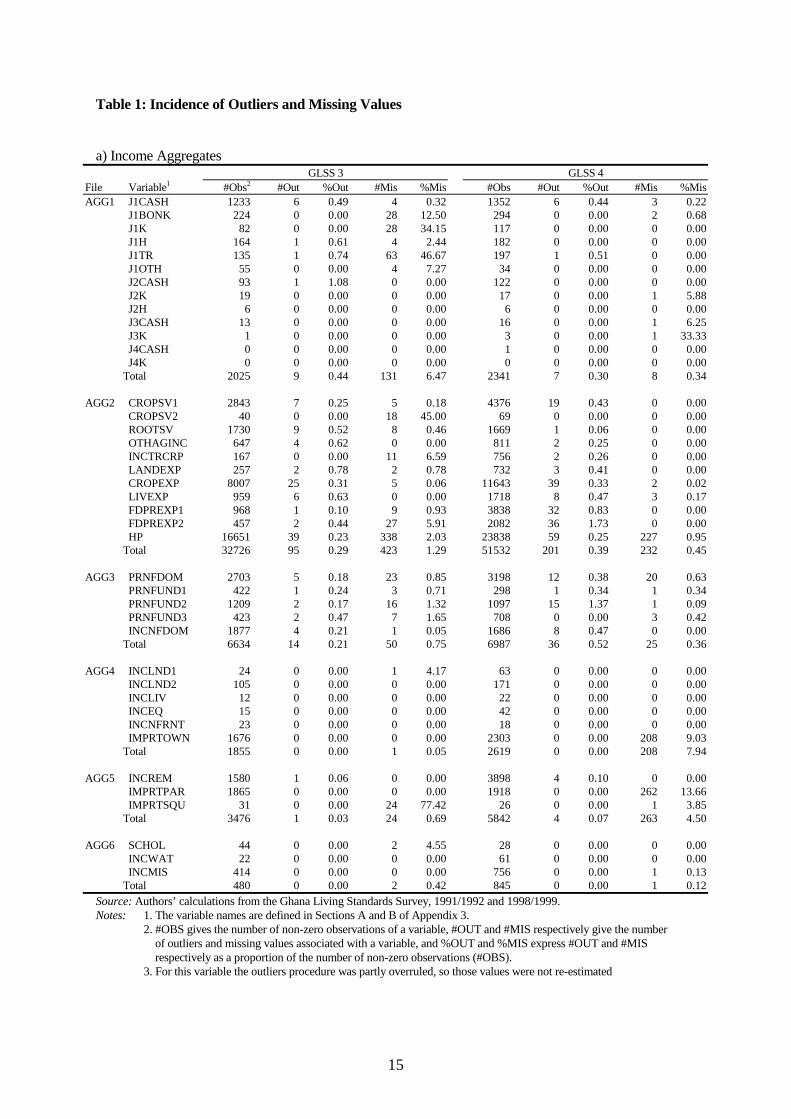
5. STATISTICAL SUMMARY OF THE GLSS 3 AND GLSS 4 ESTIMATES This section summarises some of the statistical results obtained from executing the programs on the two GLSS data sets, including a summary of the effects of the application of the procedures for treating outliers and missing values. Its purpose is not to provide an economic analysis of the results obtained, nor to provide a detailed description of the sources of incomes and components of expenditures of households. Instead, the sole purpose is to provide a broad tabular summary of the main features from a statistical viewpoint. Following our initial cleaning, the GLSS 3 data set included 4552 households which had been surveyed between the third quarter of 1991 to the third quarter of 1992, while the GLSS 4 data set contained 5998 households surveyed between April 1998 and March 1999. All incomes and expenditures are recorded in current prices, which means that no direct allowance is made for the effect of price inflation and seasonal variation on the transaction values attributed to households surveyed at different stages of each twelve month period. For present purposes this is likely to have little effect on the summary statistics because the survey was carried out in all localities and across all socio economic strata at all times throughout the year. So it may be assumed that relative differences net out. However, the effect of inflation will have an important bearing on the comparison of mean values of the various aggregates between GLSS rounds 3 and 4. (i) Outliers and missing values The incidence of outliers and missing values can be observed in Tables 1 and 2. Table 1 shows the number of outliers and missing values for each variable, that is, the number of households for which that variable was counted as an outlier or was missing, together with the number of non-zero observations for that variable. Computing outliers and missing values as a percentage of the number of non-zero observations (rather than the total number inclusive of zeros) gives a much better appreciation of their relative incidence. The variables are grouped according to the aggregates of which they form a component part, so at the aggregate level the number of observations, outliers and missing values are simply the corresponding totals of the component variables. Clearly, for some variables (and aggregates) the number of (non-zero) observations exceeds the number of households because they include more than one item. For example, FOODEXP (expenditure on food paid in cash) relates to expenditures at the individual item level. The outliers routine generates, overall, relatively few outlier values at the variable level, and this generally applies also to the numbers of outliers at the aggregate level. At the level of the aggregates the largest percentage of outliers in GLSS 3 is associated with AGG1 (income from employment) amounting to 0.44%, in GLSS 4 it is associated with AGG3 (actual and imputed rental income) amouting to 0.52%. Indeed, at the variable level only four variables show percentages of outliers in excess of 1.0% in GLSS 3 and three in GLSS 4. So it can be concluded that the outlier routine is not too invasive. As regards missing values, again in GLSS 3 the aggregate AGG1 (income from employment) figures prominently as the one most affected in terms of relative incidence, in GLSS 4 the aggregate AGG8 (expenditure on housing actual and imputed) is most affected. In GLSS 3, 6.47% of AGG1 (non-zero) observations of this aggregate were recorded as having one or more component variables missing, while in GLSS 4 the corresponding figure for AGG8 was 9.17%. These percentages conceal a considerable

13

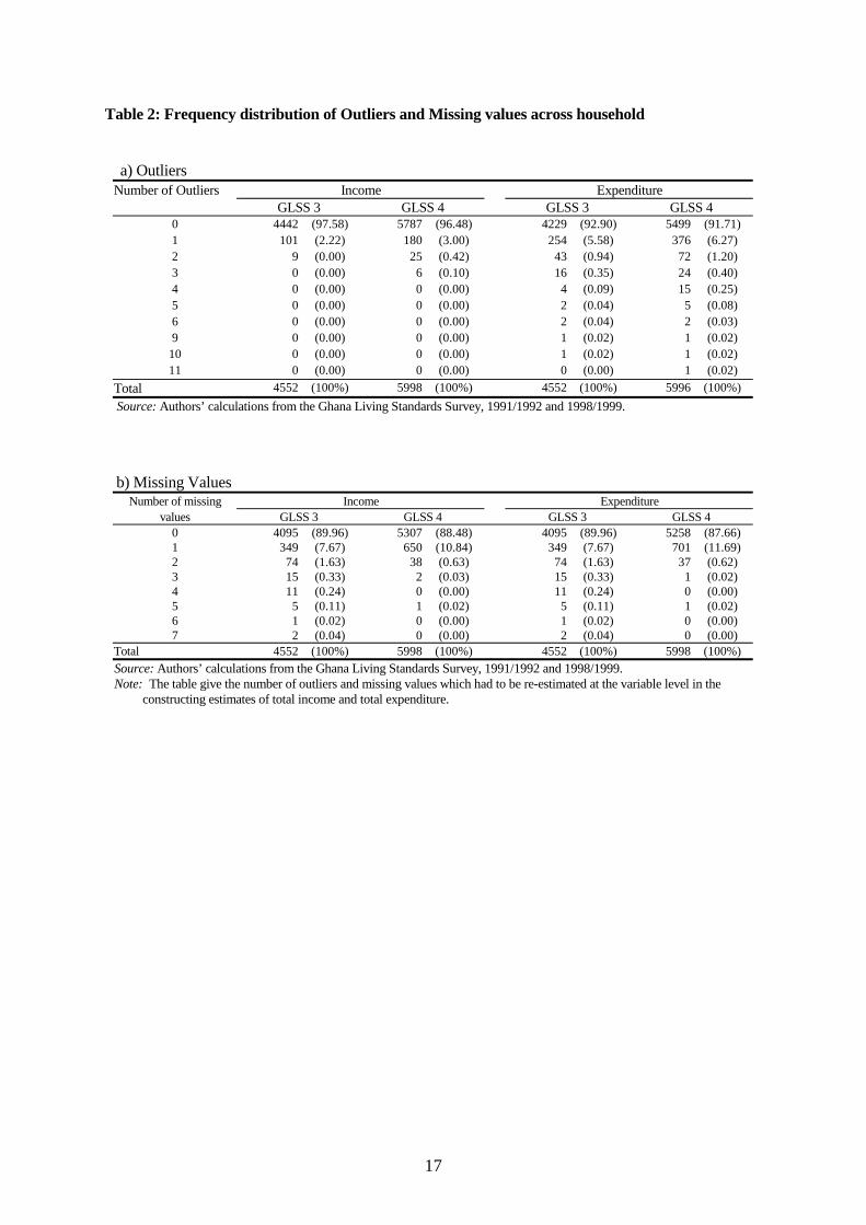
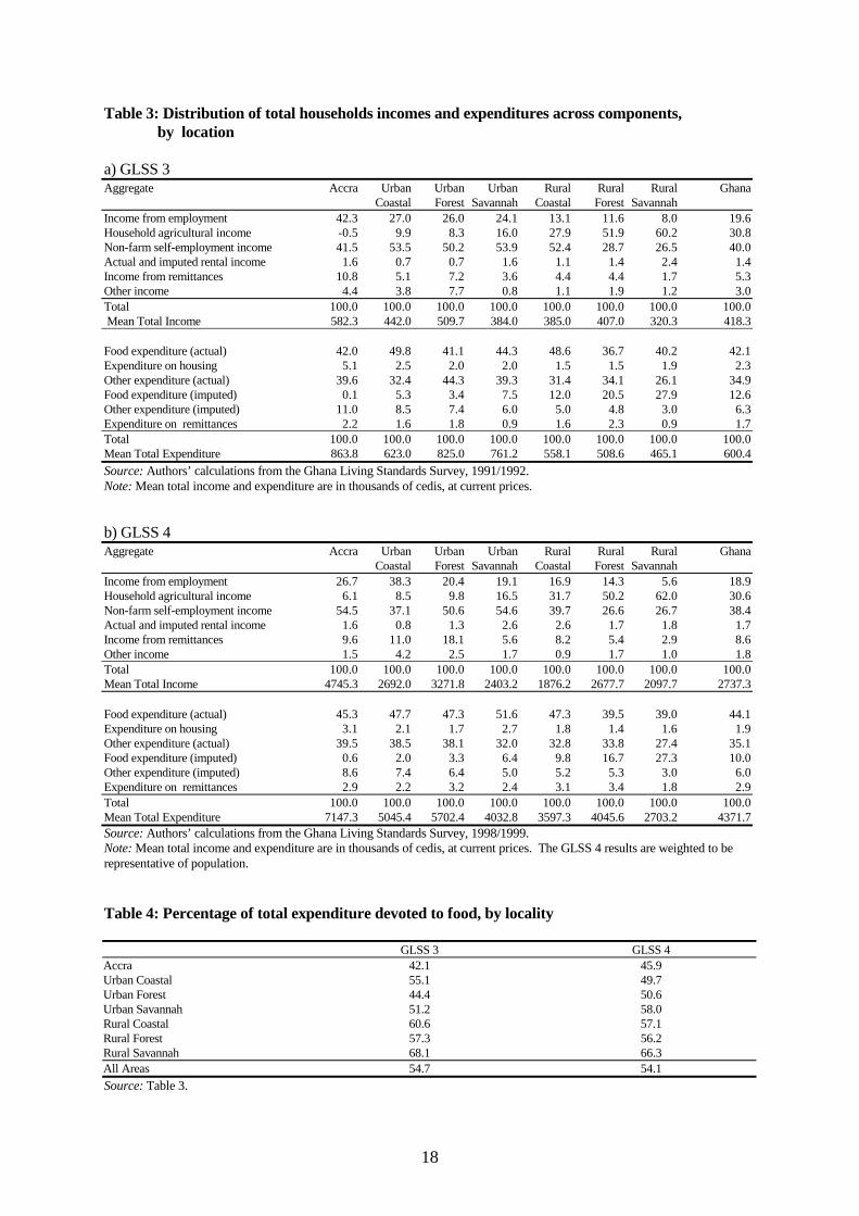
amount of variation at the variable level. For example, in GLSS 4, 35.9 perent of observations of the variable IMPRTEMP (value of imputed rental services paid by employers) were missing, although from a small number of observations. Tables 2a and 2b show the incidence of outliers and missing values affecting the estimates of total income and total expenditure as a frequency distribution across households. In order to construct this table, the variables were separately grouped according to whether they contributed to income or to expenditure aggregates. Table 2a shows the results for outliers and it can be seen that, in the case of expenditure aggregates for GLSS 3, 4529 of 4552 households (93%) were unaffected by outliers in any of the expenditure aggregates, while 254 households recorded one outlier, 43 households recorded 2 outliers, etc. When it is recalled that there are many more variables (and hence observations) for expenditures than for incomes, it is perhaps not too surprising that there are some households with 4 or more outliers in the expenditure aggregates but at most 3 outliers in the income aggregates. As regards missing values, Table 2b shows that, again, few households are affected by more than one missing value. However, unlike for outliers, the income variables are as affected by missing values than the expenditure variables and there are many cases of households contributing more than two missing values. (ii) Aggregates Table 3 shows in summary form the mean values of the twelve “standardised” income and expenditure aggregates, for each round of the surveys analysed, and these are further subdivided according to seven broad locality groups: Accra, Urban Coastal, Urban Forest, Urban Savannah, Rural Coastal, Rural Forest and Rural Savannah areas. The means are calculated over all households; in other words, they include households with zero values. Overall, across Ghana as a whole, it can be observed that the recorded mean total income rose by 555% between rounds 3 and 4 whereas mean total expenditure increased by 629%, both figures being expressed in nominal terms. Obviously, these figures would be meaningful to the extent it is possible to correct for the important inflation that occurred between the two rounds. Such figures are presented and discussed in the Poverty Profile (Ghana Statistical Service, 2000, Poverty Trends in Ghana in the 1990s). Table 3 also shows great stability in the percentages of incomes and expenditures derived from different sources. The most meaningful difference in the income side, is the income from remittances component which increases from 5.3% of total income to 8.6%. On the expenditure side, food expenditure paid in cash increase its share of total expenditure from 42.1% to 44.1%, but the imputed food expenditure declines from 12.6% to 10.0%. As a result the proportion of total expenditure devoted to food is stable overall, although its composition between the cash and the imputed part changes as seen in Table 4. These percentages shown in Table 4 are based on food and total expenditures, both of which are inclusive of actual and imputed items. These percentages are highest in rural areas and lowest in Accra, in both rounds 3 and 4, and the imputed food expenditure component is highest in rural areas and lowest in Accra, as one might expect. Differences between localities in the patterns of incomes and expenditures also reveal some degree of consistency between rounds, although the differences in these patterns between rounds are obviously affected by quite marked changes in individual aggregates as referred to earlier.

14

A broad comparison between the mean income and expenditure aggregates reveals the expected shortfall of recorded income below expenditure. The shortfall is quite pronounced, however, and the locality breakdown reveals quite marked variations between localities. The shortfall is most pronounced in Accra, and smallest in rural areas, a fact which may perhaps be explained by the relatively greater importance of imputations which are added to both incomes and expenditures of households in rural areas compared with urban areas. In any case, all of these issues require further analysis in order to identify the nature and source of any underestimation of incomes and/or overestimation of expenditures.

15

Table 1: Incidence of Outliers and Missing Values a) Income Aggregates

GLSS 3 GLSS 4 File Variable1 #Obs2 #Out %Out #Mis %Mis #Obs #Out %Out #Mis %Mis AGG1 J1CASH 1233 6 0.49 4 0.32 1352 6 0.44 3 0.22 J1BONK 224 0 0.00 28 12.50 294 0 0.00 2 0.68 J1K 82 0 0.00 28 34.15 117 0 0.00 0 0.00 J1H 164 1 0.61 4 2.44 182 0 0.00 0 0.00 J1TR 135 1 0.74 63 46.67 197 1 0.51 0 0.00 J1OTH 55 0 0.00 4 7.27 34 0 0.00 0 0.00 J2CASH 93 1 1.08 0 0.00 122 0 0.00 0 0.00 J2K 19 0 0.00 0 0.00 17 0 0.00 1 5.88 J2H 6 0 0.00 0 0.00 6 0 0.00 0 0.00 J3CASH 13 0 0.00 0 0.00 16 0 0.00 1 6.25 J3K 1 0 0.00 0 0.00 3 0 0.00 1 33.33 J4CASH 0 0 0.00 0 0.00 1 0 0.00 0 0.00 J4K 0 0 0.00 0 0.00 0 0 0.00 0 0.00 Total

2025 9 0.44 131 6.47 2341 7 0.30 8 0.34

AGG2 CROPSV1 2843 7 0.25 5 0.18 4376 19 0.43 0 0.00 CROPSV2 40 0 0.00 18 45.00 69 0 0.00 0 0.00 ROOTSV 1730 9 0.52 8 0.46 1669 1 0.06 0 0.00 OTHAGINC 647 4 0.62 0 0.00 811 2 0.25 0 0.00 INCTRCRP 167 0 0.00 11 6.59 756 2 0.26 0 0.00 LANDEXP 257 2 0.78 2 0.78 732 3 0.41 0 0.00 CROPEXP 8007 25 0.31 5 0.06 11643 39 0.33 2 0.02 LIVEXP 959 6 0.63 0 0.00 1718 8 0.47 3 0.17 FDPREXP1 968 1 0.10 9 0.93 3838 32 0.83 0 0.00 FDPREXP2 457 2 0.44 27 5.91 2082 36 1.73 0 0.00 HP 16651 39 0.23 338 2.03 23838 59 0.25 227 0.95 Total

32726 95 0.29 423 1.29 51532 201 0.39 232 0.45

AGG3 PRNFDOM 2703 5 0.18 23 0.85 3198 12 0.38 20 0.63 PRNFUND1 422 1 0.24 3 0.71 298 1 0.34 1 0.34 PRNFUND2 1209 2 0.17 16 1.32 1097 15 1.37 1 0.09 PRNFUND3 423 2 0.47 7 1.65 708 0 0.00 3 0.42 INCNFDOM 1877 4 0.21 1 0.05 1686 8 0.47 0 0.00 Total

6634 14 0.21 50 0.75 6987 36 0.52 25 0.36

AGG4 INCLND1 24 0 0.00 1 4.17 63 0 0.00 0 0.00 INCLND2 105 0 0.00 0 0.00 171 0 0.00 0 0.00 INCLIV 12 0 0.00 0 0.00 22 0 0.00 0 0.00 INCEQ 15 0 0.00 0 0.00 42 0 0.00 0 0.00 INCNFRNT 23 0 0.00 0 0.00 18 0 0.00 0 0.00 IMPRTOWN 1676 0 0.00 0 0.00 2303 0 0.00 208 9.03 Total

1855 0 0.00 1 0.05 2619 0 0.00 208 7.94

AGG5 INCREM 1580 1 0.06 0 0.00 3898 4 0.10 0 0.00 IMPRTPAR 1865 0 0.00 0 0.00 1918 0 0.00 262 13.66 IMPRTSQU 31 0 0.00 24 77.42 26 0 0.00 1 3.85 Total

3476 1 0.03 24 0.69 5842 4 0.07 263 4.50

AGG6 SCHOL 44 0 0.00 2 4.55 28 0 0.00 0 0.00 INCWAT 22 0 0.00 0 0.00 61 0 0.00 0 0.00 INCMIS 414 0 0.00 0 0.00 756 0 0.00 1 0.13 Total 480 0 0.00 2 0.42 845 0 0.00 1 0.12

Source: Authors’ calculations from the Ghana Living Standards Survey, 1991/1992 and 1998/1999. Notes: 1. The variable names are defined in Sections A and B of Appendix 3. 2. #OBS gives the number of non-zero observations of a variable, #OUT and #MIS respectively give the number

of outliers and missing values associated with a variable, and %OUT and %MIS express #OUT and #MIS respectively as a proportion of the number of non-zero observations (#OBS).

3. For this variable the outliers procedure was partly overruled, so those values were not re-estimated

16

b) Expenditure Aggregates

GLSS 3 GLSS 4 File Variable #Obs #Out %Out #Mis %Mis #Obs #Out %Out #Mis %Mis AGG7

FOODEXP 95985 100 0.10 0 0.00 153307 177 0.12 0 0.00

AGG8 IMPRTOWN 1676 0 0.00 0 0.00 2303 0 0.00 208 9.03 IMPRTPAR 1865 0 0.00 24 1.29 1918 0 0.00 262 13.66 RENTPAID 879 9 1.02 10 1.14 1183 10 0.85 10 0.85 IMPRTSQU 31 0 0.00 0 0.00 26 0 0.00 1 3.85 IMPRTEMP 67 0 0.00 0 0.00 64 0 0.00 23 35.94 Total

4518 9 0.20 34 0.75 5494 10 0.18 504 9.17

AGG9 WATB1 561 3 0.53 8 1.43 649 6 0.92 10 1.54 WATB2 854 2 0.23 12 1.41 1675 12 0.72 0 0.00 ELECB 1148 9 0.78 0 0.00 2150 7 0.33 0 0.00 GARB 69 1 1.45 8 11.59 225 22 9.78 14 6.22 EDUCEXP3 5978 0 0.00 9 0.15 8387 2 0.02 4 0.05 DAYEXPD 29726 57 0.19 0 0.00 52290 96 0.18 0 0.00 YREXP 53432 179 0.34 47 0.09 78624 294 0.37 2 0.00 MISCEXP 742 8 1.08 0 0.00 2648 9 0.34 0 0.00 Total

92510 259 0.28 84 0.09 146648 448 0.31 30 0.02

AGG10 HP 16651 39 0.23 338 2.03 23838 59 0.25 227 0.95 J1K 82 0 0.00 28 34.15 117 0 0.00 0 0.00 J2K 19 0 0.00 1 5.26 17 0 0.00 1 5.88 J3K 1 0 0.00 0 0.00 3 0 0.00 1 33.33 J4K 0 0 0.00 0 0.00 0 0 0.00 0 0.00 Total

16753 39 0.23 367 2.19 23975 59 0.25 229 0.96

AGG11 J1H 164 1 0.61 5 3.05 182 0 0.00 0 0.00 J1OTH 55 0 0.00 4 7.27 34 0 0.00 0 0.00 J2H 6 0 0.00 0 0.00 6 0 0.00 0 0.00 INCNFDOM 1877 4 0.21 1 0.05 1686 8 0.47 0 0.00 USEVAL 9806 42 0.43 79 0.81 16459 47 0.29 30 0.18 Total

11908 47 0.39 89 0.75 18367 55 0.30 30 0.16

AGG12 REMITEXP 1844 0 0 0 0.00 4377 2 0.05 0 0.00 Source: Authors’ calculations from the Ghana Living Standards Survey, 1991/1992 and 1998/1999. Notes: 1. The variable names are defined in Sections A and B of Appendix 3. 2. #OBS gives the number of non-zero observations of a variable, #OUT and #MIS respectively give the number of outliers and missing values associated with a variable, and %OUT and %MIS express #OUT and #MIS respectively as a proportion of the number of non-zero observations (#OBS). 3. For this variable the outliers procedure was partly overruled, so those values were not re-estimated .

17

Table 2: Frequency distribution of Outliers and Missing values across household a) Outliers

Number of Outliers Income Expenditure GLSS 3 GLSS 4 GLSS 3 GLSS 4

0 4442 (97.58) 5787 (96.48) 4229 (92.90) 5499 (91.71) 1 101 (2.22) 180 (3.00) 254 (5.58) 376 (6.27) 2 9 (0.00) 25 (0.42) 43 (0.94) 72 (1.20) 3 0 (0.00) 6 (0.10) 16 (0.35) 24 (0.40) 4 0 (0.00) 0 (0.00) 4 (0.09) 15 (0.25) 5 0 (0.00) 0 (0.00) 2 (0.04) 5 (0.08) 6 0 (0.00) 0 (0.00) 2 (0.04) 2 (0.03) 9 0 (0.00) 0 (0.00) 1 (0.02) 1 (0.02)

10 0 (0.00) 0 (0.00) 1 (0.02) 1 (0.02) 11 0 (0.00) 0 (0.00) 0 (0.00) 1 (0.02)

Total 4552 (100%) 5998 (100%) 4552 (100%) 5996 (100%) Source: Authors’ calculations from the Ghana Living Standards Survey, 1991/1992 and 1998/1999. b) Missing Values

Number of missing Income Expenditure values GLSS 3 GLSS 4 GLSS 3 GLSS 4

0 4095 (89.96) 5307 (88.48) 4095 (89.96) 5258 (87.66) 1 349 (7.67) 650 (10.84) 349 (7.67) 701 (11.69) 2 74 (1.63) 38 (0.63) 74 (1.63) 37 (0.62) 3 15 (0.33) 2 (0.03) 15 (0.33) 1 (0.02) 4 11 (0.24) 0 (0.00) 11 (0.24) 0 (0.00) 5 5 (0.11) 1 (0.02) 5 (0.11) 1 (0.02) 6 1 (0.02) 0 (0.00) 1 (0.02) 0 (0.00) 7 2 (0.04) 0 (0.00) 2 (0.04) 0 (0.00)

Total 4552 (100%) 5998 (100%) 4552 (100%) 5998 (100%) Source: Authors’ calculations from the Ghana Living Standards Survey, 1991/1992 and 1998/1999. Note: The table give the number of outliers and missing values which had to be re-estimated at the variable level in the constructing estimates of total income and total expenditure.

18

Table 3: Distribution of total households incomes and expenditures across components, by location a) GLSS 3 Aggregate Accra Urban

Coastal Urban Forest

Urban Savannah

Rural Coastal

Rural Forest

Rural Savannah

Ghana

Income from employment 42.3 27.0 26.0 24.1 13.1 11.6 8.0 19.6 Household agricultural income -0.5 9.9 8.3 16.0 27.9 51.9 60.2 30.8 Non-farm self-employment income 41.5 53.5 50.2 53.9 52.4 28.7 26.5 40.0 Actual and imputed rental income 1.6 0.7 0.7 1.6 1.1 1.4 2.4 1.4 Income from remittances 10.8 5.1 7.2 3.6 4.4 4.4 1.7 5.3 Other income 4.4 3.8 7.7 0.8 1.1 1.9 1.2 3.0 Total 100.0 100.0 100.0 100.0 100.0 100.0 100.0 100.0 Mean Total Income 582.3 442.0 509.7 384.0 385.0 407.0 320.3 418.3 Food expenditure (actual) 42.0 49.8 41.1 44.3 48.6 36.7 40.2 42.1 Expenditure on housing 5.1 2.5 2.0 2.0 1.5 1.5 1.9 2.3 Other expenditure (actual) 39.6 32.4 44.3 39.3 31.4 34.1 26.1 34.9 Food expenditure (imputed) 0.1 5.3 3.4 7.5 12.0 20.5 27.9 12.6 Other expenditure (imputed) 11.0 8.5 7.4 6.0 5.0 4.8 3.0 6.3 Expenditure on remittances 2.2 1.6 1.8 0.9 1.6 2.3 0.9 1.7 Total 100.0 100.0 100.0 100.0 100.0 100.0 100.0 100.0 Mean Total Expenditure 863.8 623.0 825.0 761.2 558.1 508.6 465.1 600.4 Source: Authors’ calculations from the Ghana Living Standards Survey, 1991/1992. Note: Mean total income and expenditure are in thousands of cedis, at current prices. b) GLSS 4 Aggregate Accra Urban

Coastal Urban Forest

Urban Savannah

Rural Coastal

Rural Forest

Rural Savannah

Ghana

Income from employment 26.7 38.3 20.4 19.1 16.9 14.3 5.6 18.9 Household agricultural income 6.1 8.5 9.8 16.5 31.7 50.2 62.0 30.6 Non-farm self-employment income 54.5 37.1 50.6 54.6 39.7 26.6 26.7 38.4 Actual and imputed rental income 1.6 0.8 1.3 2.6 2.6 1.7 1.8 1.7 Income from remittances 9.6 11.0 18.1 5.6 8.2 5.4 2.9 8.6 Other income 1.5 4.2 2.5 1.7 0.9 1.7 1.0 1.8 Total 100.0 100.0 100.0 100.0 100.0 100.0 100.0 100.0 Mean Total Income 4745.3 2692.0 3271.8 2403.2 1876.2 2677.7 2097.7 2737.3 Food expenditure (actual) 45.3 47.7 47.3 51.6 47.3 39.5 39.0 44.1 Expenditure on housing 3.1 2.1 1.7 2.7 1.8 1.4 1.6 1.9 Other expenditure (actual) 39.5 38.5 38.1 32.0 32.8 33.8 27.4 35.1 Food expenditure (imputed) 0.6 2.0 3.3 6.4 9.8 16.7 27.3 10.0 Other expenditure (imputed) 8.6 7.4 6.4 5.0 5.2 5.3 3.0 6.0 Expenditure on remittances 2.9 2.2 3.2 2.4 3.1 3.4 1.8 2.9 Total 100.0 100.0 100.0 100.0 100.0 100.0 100.0 100.0 Mean Total Expenditure 7147.3 5045.4 5702.4 4032.8 3597.3 4045.6 2703.2 4371.7 Source: Authors’ calculations from the Ghana Living Standards Survey, 1998/1999. Note: Mean total income and expenditure are in thousands of cedis, at current prices. The GLSS 4 results are weighted to be representative of population. Table 4: Percentage of total expenditure devoted to food, by locality GLSS 3 GLSS 4 Accra 42.1 45.9 Urban Coastal 55.1 49.7 Urban Forest 44.4 50.6 Urban Savannah 51.2 58.0 Rural Coastal 60.6 57.1 Rural Forest 57.3 56.2 Rural Savannah 68.1 66.3 All Areas 54.7 54.1 Source: Table 3.

19

APPENDIX 1: SOURCES AND METHODS FOR THE CALCULATION OF INCOME AND EXPENDITURE AGGREGATES

A detailed description of how the income and expenditure aggregates were constructed from the variables collected by the GLSS questionnaire is set out below. As explained in Section 4 of the text, the method used was to calculate incomes and expenditures at a highly disaggregated level and to construct the aggregates listed in the text by summation over individuals, commodities or other categories as appropriate. In most cases the subaggregates required could be derived directly from the survey responses; only a few involved more complicated or subjective estimation or imputation, such as imputations of rent, estimation of the depreciation of capital assets and of the use values of durable goods. All estimates relate to a twelve-month time period even though they have often been calculated by grossing up survey responses relating to a shorter time period. Such calculations will be clear in the details shown below. In some instances there is sufficient information available from the survey to derive more than one estimate of the subaggregates. These may be viewed either as providing a consistency check and hence as some measure of accuracy of one a priori preferred estimate or as a means of arriving at an overall estimate which might be some combination of the two estimates. The treatment differed according to the subaggregate in question, and details are given in the relevant section below. Questions in the survey questionnaire are referred to as in the following examples: S5BQ10 relates to question 10 in Section 5B, S4Q11 to question 11 in Section 4, etc. Although both questionnaires (GLSS 3 and GLSS 4) are very similar, some of the sections and therefore the question references are different. We are using the GLSS 4 questionnaire in the following description. (1) Income from employment This category of income is more generally referred to as employee compensation. The survey elicits responses on up to four jobs undertaken in the past twelve months. For individuals whose primary job of the past twelve months involved working as an employee of a non-household individual or enterprise (this being deduced from S4BQ4), income received in cash, in kind and as bonuses from this job were calculated. Monetary payment in a given time unit (chosen by the respondent) is recorded (S4BQ6) as is the value of any bonuses received (S4BQ12); the value of bonuses was only included in the final aggregate when this was reported as being additional to the previously stated cash payment. The value of these two types of earnings over the past twelve months was estimated using the information on time spent at work (S4BQ7 in the same time unit chosen by the respondent in the question S4BQ6). Regarding payment in kind, information is collected on the value of remuneration received in a specified time unit in the forms of food/animals, subsidised housing, subsidised transport and other forms is given (S4BQ15, S4BQ17, S4BQ19, S4BQ21 respectively). Some individuals may have had a secondary activity in the past twelve months which provided some employment income (as opposed to self employment income, this determined by question S4CQ12). For such individuals figures for payment in money and total payment in kind were calculated by multiplying the amounts received in a given time unit (S4CQ10 and S4CQ15 respectively) by the time spent on the job in the previous year, measured in the same time units (weeks per year, S4CQ6; hours per week, S4CQ7). The

20

same procedure was used to calculate the employment income from a third (from S4DQ9, S4DQ14 multiplying by the amount received in a given unit of S4DQ5, weeks per year and S4DQ6, hours per week) and a fourth occupation (from S4EQ9, S4EQ14 multiplying by the amount received in a given unit of S4EQ5, weeks per year and S4EQ6, hours per weeks). The sum of employment income from the primary, secondary, tertiary and quaternary jobs of the past twelve months provides an estimate of annual employment income at the individual level. Of course, annual employment income is liable to be underestimated for many individuals. (2) Household agricultural income (i) Revenues The revenue from the sale of crops was estimated for each crop by the value of the sales given by the respondent (S8CQ8 and S8CQ11). Revenue from the sale of roots, fruits and vegetable are estimated for each category by the value of the sales in the last two weeks (S8CQ26) and annualized. Revenue from other agricultural income in cash or in kind are also taken into consideration (S8EQ1-9). For food products made by processing or transforming homegrown crops, the revenue for each category was estimated by the value of the sales in the last two weeks (S8GQ12) and then annualised. Finally, a valuation of domestic consumption of own agricultural production should be included. In GLSS 3 information on domestic consumption of own agricultural production for each household was collected using seven recalls at two-day intervals in rural areas, and ten recalls at three-day intervals in urban areas. In GLSS 4, the number of recall periods was standard at five across all areas; with a recall of five days. This estimate is calculated without the enumerator’s first visit which is unbounded and seen as less precise compared to the other bounded recall periods (S8HQ4-8). The individual quantities recorded are then multiplied by the value of each item (S8HQ10), summed across the period for each food item, and then multiplied up by 365/27 (GLSS 3, urban), 365/12 (GLSS 3, rural) or 365/25 (GLSS 4). These annual estimates were then summed across all food items to give the estimate of the household’s annual expenditure on imputed food. Thus the usual problem of imputing the value of such consumption is circumvented because respondents are asked to value their consumption at market prices. Of course, this valuation may not be very reliable, but it will almost certainly be more reliable than an attempt to impute the opportunity cost without access to detailed local price information. These different types of revenues were aggregated over all commodities in each case and then summed to give agricultural revenue at the household level. Admittedly, this may exclude some items which ought to be classified as revenue such as the value of output paid as factor income or given away. However such revenues would also appear as costs and would therefore cancel out when the net income figure is calculated, so their omission ought not to affect the final estimate. (ii) Costs

21

Current rental expenditure on land over the past twelve months is given directly (S8BQ9). This figure does, however, include rental payments made as part of a sharecropping or similar arrangement, and it is unfortunately not possible to identify such instances. Strictly, rental payments made by sharecroppers should not be included among the costs since the value of the corresponding output is unlikely to be included among the revenues. Net household agricultural income will thus be understated for households farming as sharecroppers if the associated rental payments have been deducted. Such arrangements tend to be most prevalent in the traditional sector, especially cocoa production. But since overall the majority of rental payments are made in monetary form, it was decided to include rental payments on land among agricultural costs for all households. An alternative approach would have been to assume that all farming households operating primarily in the traditional sector are sharecroppers, while those in the modern sector pay rent in cash (again the availability of the subaggregates enables users to redefine the aggregate in this way if they so wish). Expenditure over the past twelve months on a wide range of inputs for crop production is directly given by (S8FQ2). Expenditure on labour and other costs over the past two weeks on inputs for producing transformed food products is recorded for each category of product (S8GQ7, S8GQ9 respectively), and is included in the costs side of the production account, assuming these expenditures to be additional to those on inputs for crops. These last two expenses categories needed to be annualised. Current expenditures over the past twelve months on nine categories of inputs for livestock rearing and fishing are also included (S8FQ2). Finally, depreciation of farm equipment was estimated geometrically with a depreciation rates estimated based on Ghanaian accounting conventions on the time taken for “full depreciation” of an asset.7 Full depreciation was taken to mean the reduction of an asset to 10% of its initial value. The value of depreciation expenses over the past year was then estimated by multiplying the current value of an item of equipment (S8AQ35) by the factor δi/(1 - δi) for items with a depreciation rate of δi for item i. The assumed annual geometric depreciation rates for different items of agricultural equipment are show below, along with the corresponding write-off period in years. Depreciation rates of agricultural equipment Item of farm equipment Depreciation rate (%) Write-off period

Tractors 25 % 8 years

Ploughs 54 % 3 years

Trailers/carts, farm vehicles (excluding tractors) 40 % 4-5 years

Other animal and other tractors drawn equipment, sprayers, net, safety equipment and other farm equipment.

35 % 5-6 years

Source: National Accounts, Ghana Statistical Service.

If anything, these depreciation allowances are likely to be overstated (and hence profits correspondingly understated), being based on an accounting convention (which is typically conservative in this area). However, because of the element of arbitrariness in the estimation

7 We are grateful to Dr. K.A. Twum-Baah and Mr. Oti Duah of the Ghana Statistical Service for supplying us with this information on Ghanaian accounting conventions, both for agricultural equipment and for the assets of non-farm enterprises.

22

of depreciation, gross income from agricultural activity and the estimate of depreciation have been recorded separately; thus net income may be estimated as the difference between the former and the latter. Gross income was calculated as the sum of the revenues (including the valuation of domestic consumption) minus all of the input costs specified above (other than depreciation). It is also possible to make a second estimate of agricultural income using information in Section 4 (labour) and Section 8H (home-produced food consumption) of the survey. Payment in monetary form received by household members is recorded for their first, second, third and fourth occupation in the past twelve months, irrespective of whether this income was earned from wage employment or self-employment. For each individual the total of each of these money incomes earned by working in agricultural self employment can be estimated. An estimate of household agricultural income may be computed by aggregating this estimate of agricultural self-employment income across all household members, and adding the value of any consumption of home produced food. Such an estimate is likely to be unreliable, and the former is preferred for present purposes; however, both have been estimated and included in the data set, as well as the estimate of depreciation. (3) Non-farm self employment income Information is provided for each of up to three enterprises owned and operated wholly or partially by the household. Three estimates of this aggregate have been made, each of which are recorded. The most obvious approach is to compute the difference between total revenues and total (current) costs, and to aggregate this over all enterprises owned by the household. Total revenues consist of payments received in cash or in kind as well as the value of any output consumed domestically. For enterprises which were operational in the two weeks between the two survey interviews, revenue received in cash and revenue received in kind were estimated by multiplying revenue received in the past two weeks (S10DQ1, S10DQ3 respectively) by 365/14 multiplied by the proportion of the year for which the enterprise operated (S10AQ6/12). The estimate of the value of domestic consumption of output was similarly based on the estimated value of such consumption in the past two weeks (S10DQ5). One slight problem with the latter is the vagueness of the question which means that it is not clear whether domestic consumption is valued at producer or market prices by respondents; also it does not allow the distinction to be drawn between consumption of output and consumption of input stocks. For enterprises which did not operate in the two weeks preceding the interview a question is asked on total revenue in cash and in kind usually received during a two week period (S10DQ6). This was converted into an annual value by multiplying by the product of 365/14 and the proportion of the year for which the enterprise operated (S10AQ6/12 again). The estimate of the value of the domestic consumption of output was similarly based on the estimated value of such consumption that is usually consumed by the household over a two week period (S10DQ10). The costs that should be deducted from these revenues are total current input expenditures and (if net income is to be estimated) an estimate of depreciation of fixed capital. The former is calculated by working out expenditure for each enterprise on each of 14 categories of inputs by multiplying the expenditures (S10BQ5 or S10BQ6 or S10CQ7) by the appropriate annualisation factor and by the number of months for which the enterprise operated (S10AQ6) expressed as a fraction of 12. Enterprises that did not operate in the past two

23

weeks, there expenditures were calculated in the same manner using questions S10BQ12-14. Depreciation allowances were estimated from the current market value of the assets in question (S10CQ2) in the same manner as with agricultural capital items. The depreciation rates used were again based informally on Ghanaian accounting conventions in the same way as described for agricultural equipment. In line with standard practice it was assumed that the depreciation rate of stocks of unsold goods was zero. As in the case of agricultural income, gross income and estimated depreciation have been recorded, so that net income may be calculated as the difference between these items. In practice, as noted in the text above (page 5), and in common with the experience of LSMS questionnaires in other African countries, this estimate clearly gives a major underestimation of income from this source; a majority of the resulting income estimates are found to be negative, often significantly so. A number of possible explanations may be advanced for this massive underestimation. For example, expenditures on inputs may be overstated due to double-counting in instances in which an input purchased primarily for one enterprise is used for other enterprises or for domestic purposes; also it is possible that some of the input expenditures made in kind should have a counterpart on the revenue side which is not recorded (i.e. if payment is made in the form of the enterprises' own products). Another possibility is that the revenue figures supplied by respondents may already be quoted net of input expenditures (or at least some input expenditures) in many cases. In view of these problems, two alternative estimates of non-farm self employment income have been made. One such estimate was calculated using the direct responses on the profits of enterprises. The value of net revenue used for household purposes and the value of any “retained” profits after these household expenditures have been made are recorded in the questionnaire (S10EQ1, S10EQ4, S10EQ6 and S10EQ8), each for a time period chosen by the respondent. These were converted into monthly values, from which annual figures were estimated by multiplying by the number of months in which the enterprise was operating. This second estimate of non-farm self employment income was then calculated by adding the value of domestic consumption of the output of each of the enterprises, on the assumption that this would not have be taken into account in the profit figures reported by respondents. The resulting estimate of profits is presumably gross in the sense that it does not allow for capital consumption, as it is highly unlikely that depreciation will have been taken into account in the responses, so net profits may be obtained by deducting the depreciation estimate. However, this second estimate of non-farm self-employment income will not be totally satisfactory either, partly because of the difficulty respondents are likely to have in estimating the profits of these unincorporated enterprises and partly because the questionnaire does not ask about the extent of the losses made by non-profitable enterprises. A third estimate of non-farm self-employment income (again expressed gross) may be made from the responses on self-employment income in Section 4 in all cases in which the indicated occupation is anything other than agriculture. Having identified such instances, annual self-employment income may be estimated in an exactly analogous manner to that used for agricultural self employment income above. Individuals may undertake more than one non-agricultural self-employment activity, so that in general self employment income should be added over first, second, third and fourth occupations.

24

These self-employment incomes were aggregated over all individuals in the household, and was added to the value of domestic consumption of output, calculated as above. All three estimates of gross incomes have been recorded along with the estimate of depreciation to allow users to choose which estimate to use, and whether income should be gross or net. As noted above the resulting estimates suggest that the second and third method of estimation, while probably still subject to significant error, give much more credible results. (4) Actual and imputed rental income This component comes from the rental of farming :income received from land (S8AQ15), from sharecropping (S8AQ18), from renting livestock (S8AQ31) and from leasing farm equipment (S8AQ37) and from non-farming equipment (S10DQ12) over the past twelve months; where the latter needs to be aggregated over different types of equipment. The sum of these latter incomes is likely to be an underestimate in many cases, as it does not cover all possible sources of rental income. It also includes an imputation of rent for owner-occupied dwellings. The imputations have been made based on the predictions of a hedonic regression equation, which was estimated by regressing rental values of dwellings on indicators of their characteristics and amenities, the rental values used for the dependent variable is the actual rental values (for renting households). A single hedonic equation was estimated for each round covering all localities in order to have a large number of observations, but including both locality and time period dummy variables, the latter on a monthly basis given the high rate of inflation. Besides these dummy variables, the other explanatory variables included were indicators of the size, quality of construction and amenities of the dwelling. The results – in case of GLSS 4 – are presented in Appendix 2. This income component is then calculated by the simple addition of the actual and imputed rental elements. (5) Income from remittances For remittances in the form of cash, food or other goods, the respondent is asked to record the value of each remittance received in the past twelve months (S11BQ9, S11BQ10, S11BQ11 respectively). These different transfers were summed to give an estimate of the total value of such remittances received. There is, however, the possibility that these responses will include capital as well as current remittances, a problem for which no obvious correction can be made8. Only remittances made by non-members of the household (absent or not) had been taken into account. For transfers received in the form of subsidised or free housing provided by other households, whether voluntarily or involuntarily (as in the case of squatters), the hedonic equation referred to under component (4) above has again been used to estimate the rental value of the household's dwelling given its characteristics. Unfortunately, however, in the case of partially subsidised housing, no information is available on the percentage of subsidy provided; such cases have had to be treated in the same way as rent-free provision of housing, 8 There is a question in the survey about whether some or all of the remittance is due to be repaid, but even when the response is positive the proportion of the remittance to be repaid is unknown. All remittances have been treated as current transfers, although a small minority might be partially or fully capital transfers.

25

that is assuming a transfer equal in magnitude to the entire rental value of the dwelling. In these cases the magnitude of the implicit transfer will certainly be overestimated, but the necessary information to correct for this overestimation is not available (a corresponding overestimation will also be made on the expenditure side in these cases). The component is calculated as the sum of the values of these two different types of inter-household transfers. (6) Other income This component includes an estimate of household income received from educational scholarships, derived from the education section of the questionnaire (Section 2), plus various miscellaneous incomes reported in Section 11C. Information on educational scholarships is collected at the individual level (S2AQ16), so that the household level estimate of this element is derived by aggregating these responses over all household members. In addition to income from scholarships, incomes in cash or in kind from the following sources reported in the “miscellaneous income” section of the questionnaire are also included in this component: social security (S11CQ1); state pension (S11CQ2); other income from central government (S11CQ3); retirement benefits (S11CQ4) or other income from other sources excluding Susu (S11CQ6). Each of these is directly recorded in the survey responses. Dowry or inheritance (S11CQ5) was dropped from the calculation as it should be seen as a capital transfer more than an income. It should be noted that the contents of the “other income from other sources excluding Susu” category are unclear and there remains the possibility that some capital receipts will be included in addition to current incomes. (7) Food expenditure (actual) In GLSS 3 information on food expenditures for each household was collected using seven recalls at two-day intervals in rural areas, and ten recalls at three-day intervals in urban areas. In GLSS 4, the number of recall periods was standard at five across all areas; with a recall of five days. This estimate is calculated without the enumerator’s first visit which is unbounded and seen as less precise compared to the other bounded recall periods (S9BQ2-6). The individual amounts recorded were summed across the period for each food item, and then multiplied up by 365/27 (GLSS 3, urban), 365/12 (GLSS 3, rural) or 365/25 (GLSS 4). These annual estimates were then summed across all food items to get the estimate of the household’s annual expenditure on food. It should be noted that alcohol and tobacco items were recorded in the same section as food items, but were transfer to non-food aggregates during the computing process. Since no account is taken of the number of months when a particular food item is purchased, the estimate of each household’s annual expenditure on an individual food item is likely to be over-estimated for those households which did purchased the food item during the survey period, but which do not purchase it in all months of the year. However, this over-estimate for some households will be counterbalanced by a corresponding under-estimation for those households which do consume the food item in some months although they did not consume any during the survey period. Although the overall variation between households will be exaggerated, the estimate of total and mean household expenditure should be unbiased, since the survey work was spread throughout the year.

26

(8) Expenditure on housing This component includes actual expenditure on rent by households, plus a series of imputations, each of which have a counterpart on the income side. Actual rent includes both payments in cash (S7CQ1) and in kind (S7CQ3), which are estimated by annualizing the values provided by respondents by simply multiplying by the appropriate factor given the time units used by respondents. Among the imputed rents, the value of housing subsidies paid by employers is estimated in the same way as on the income side (see under component (1)); all other imputations are estimated based on the predictions of the hedonic rental equation previously referred to (see under component (4)). These latter imputations cover the case of owner-occupied dwellings, cases in which a household's dwelling is provided by a relative or other private individual on a rent-free or subsidised basis, and cases in which the household claims neither to rent nor to own their dwelling. The overall expenditure component is calculated as the sum of all these different types of actual and imputed rent, although in the vast majority of cases only one of them is applicable to any one household. (9) Other expenditure (actual) This is an aggregation of three different types of expenditure, as follows. (i) Expenditure on household utilities This includes expenditure on water, electricity and garbage disposal. Respondents give the amount of their last water bill and the time period covered (S7DQ4) from which the amount of expenditure was annualized. It is also necessary to take into account the possibility that the household may have paid to acquire water from a private water vendor, a neighbour or a standpipe. This second component of expenditure on water is calculated by the amount paid to these outlets in the past two weeks (S7DQ5) and is then annualized. Annual expenditure on electricity was estimated by annualizing the amount of the last bill and the time period covered (S7DQ9). Similarly, annual expenditure on garbage disposal was estimated by the amount of the respondents last bill (S7DQ12). Each of these estimates will overstate the cross household variance (though hopefully not the mean) if the last bill happens to be atypical; one cause of this could be due to seasonal factors. (ii) Expenditure on education Various expenditures on education (school and registration fees; contributions to parents'/teachers’ associations; uniforms and sports clothes; books and school supplies; transport to and from school; food, board and lodging at school; other educational expenditure; other in-kind expenses) are recorded for each individual over the past 12 months (S2AQ6-13).9 Expenditure on education was therefore estimated by aggregating the different items of expenditure referred to above and summing over individuals in the household. (iii) Daily and annual expenses Daily expenses relate to non-food items which will typically be purchased on a frequent basis. For those items expected to be purchased frequently, information was sought by the interviewer during each visit to the household on the amount spent since the last visit; there 9 Note that it is implicitly assumed that any educational scholarships received are used to finance these items of educational expenditure, so that it would not be appropriate to view these scholarships as generating an additional imputed expenditure.

27

were thus seven recall periods in rural areas, each of two days, and 10 recall periods in urban areas, each of three days. In GLSS 4, the number of recall periods was standard at five across all areas; with a recall of five days. This estimate is calculated without the enumerator’s first visit which is unbounded and seen as less precise compared to the other bounded recall periods (S9A2Q2-6). The cross household variance of these expenditures will again be overstated if items in a category are only infrequently purchased i.e. less than once a fortnight, or if their expenditure pattern exhibits seasonality. Annual expenses relate to non-food items purchased less frequently and not included elsewhere. Expenditure on those goods are recorded for the past 12 months (S9A1Q1). Each of the items in Section 9A1 of the questionnaire has been included in this component with the exception of furniture and fixtures, including floor coverings (405- 409), appliances (411- 415 and 417), hospital expenditure accommodation (511), transport and communication (601- 603), and recreation, entertainment, education and cultural service (701-704). Those categories excluded have been already taken account of elsewhere, or represent capital, not current, expenditure. These “annual expenditures” were recorded during a single visit. (10) Food expenditure (imputed) This comprises an imputation of the consumption by households of home-produced food, plus the value of any wage income received by household members in the form of food, the latter being aggregated over all individuals in the household. Each is estimated as on the income side (see under components (2) and (1) respectively). (11) Other expenditure (imputed) This is analogous to component (10), including both household consumption of home-produced non-food items and wage income in kind paid in forms other than food or housing (the categories of subsidised transport and other forms referred to under component (1) above), but additionally includes an imputation of the consumption flow derived by households from consumer durable goods they own. The former elements have been estimated as on the income side (see under components (3) and (1) above); the latter has been estimated based on the depreciation of the consumer durable goods, assuming a geometric rate of 20% per annum. The choice of this rate was arbitrary; an attempt was made to use information available in the questionnaire on the age, purchase value and current value of durable goods to estimate average depreciation rates for each good, but this gave highly unsatisfactory results, probably due to the very high and variable rates of inflation over recent years in Ghana. The 20% depreciation rate was therefore adopted, and the flow of consumption services derived from a durable good was therefore estimated as one quarter (0.2/(1 - 0.2)) of its current value (from S12BQ4). Four items (house, land, shares and boat) were deleted as they cannot be considered as consumer durable goods. Furthermore, two other items (canoes and outboard motors) were not recorded in this aggregates, but in aggregate 2 since they should be seen as farm assets. (12) Expenditure on remittances The value of each of the remittances made by households in the previous year is recorded by the amount of cash (S11AQ10), the value in food (S11AQ11) and the value in goods (S11AQ12). The figure for total remittances was calculated as the sum of these factors.

28

APPENDIX 2: ESTIMATION OF IMPUTED RENTAL VALUES FOR HOUSING The widely accepted accounting practice suggested by the United Nations (A System of National Accounts, UN 1993) views the inhabitants of owner-occupied housing as the owners of a productive asset from which they derive consumption value. This is usually treated as its rental value and is added to both the income and expenditure sides of the current account. Moreover, in most developing countries, a non-negligible proportion of households receive their dwellings free of charge (or at a non-cost-recovery fee) from either their family or their employer, and a few are squatters. For example, in the fourth round of GLSS, 42 percent of households owned their dwelling, while 20 and 2 percent respectively obtained it from their family or their employers, and less tham one percent were squatters, the remaining 36 percent being households who paid a rent. In the third and fourth round of the GLSS, information can be obtained for only one of these groups: the amount paid by households who rent (tenants). No information at all is provided by the questionnaire for 64 percent of households, and it is desirable to impute a value in these cases to reflect the housing services which these households are receiving. One way to approximate the rental market value of their dwelling is to estimate an hedonic equation relating the information on rental values of rented to their characteristics and amenities. This equation can then be used to impute a value to the remainder of our sample given the available information on the characteristics and amenities of each dwelling. ESTIMATION OF THE HEDONIC EQUATION Using the Ordinary Least Squares technique, we specify an equation in which the annualized rental value of a dwelling (previously cleaned of any outliers), is a function of three groups of variables: the location, time of interview and the characteristics and amenities of the dwelling. The location variables correspond to one of the following seven areas: Accra, Urban Coastal, Urban Forest, Urban Savannah, Rural Coastal, Rural Forest or Rural Savannah. These location variables should capture part of the differentials in land values . The time variables are linked to the month in which the interview took place and capture inflation. It should be noted that the time coefficients were not used directly, but were used instead to estimate the coefficient on a trend variable in housing price, thereby implying a smooth evolution of rental values over time. Finally, a list of dwelling characteristics and amenities was included such as the type of light and water sources, type of toilets, and whether the floor is in concrete or tiled, as well as the size of the dwelling. It must be noted that, except for the size of the house, all these variables are dichotomous (e.g. a variable takes the value 1 if the dwelling has piped water or 0 if not). This technique has the advantage of using all the information available to get an estimate of the value of housing services, but also has some drawbacks. In rural areas there are only a few rented dwellings, hence few observations. Table A2.1 presents the regression results, in case of GLSS 4. The fit of the equation at 45% is respectable for cross-section data. Since the dependent variable is in logarithmic form, all the coefficients of the dichotomous variables can be interpreted as their effect in percentage terms on housing rent. For example, a coefficient of 1.227 for Accra means that dwellings in Accra are on average 123 per cent more costly to rent, after having controlled for the other variables. The imputed rent derived from prediction based on this regression is presented in Table A2.2 below.

29

Since, by definition, the regression technique produces a smooth imputation, the outlier procedure was only applied on the actual rent paid by tenants and not to the imputed component. However, missing values, which result from one or more of the explanatory variables being missing for the household in question, were re-estimated in the usual way as the locality mean value. The resulting imputations, plus the estimates of actual rental payments, form the basis of the “Expenditure on Housing” aggregate, and, for each imputed expenditure, corresponding imputations are included among the income aggregates. Appendix 1 provides further details on the treatment of the imputations relating to housing on the income side of the current account. Table A2.1: Regression results from hedonic equation Variable Coefficient t-Ratio Constant 8.989 30.269 Accra 1.227 8.175 Urban Coastal 0.301 1.964 Urban Forest 0.444 3.014 Urban Savannah 0.560 3.448 Rural Coastal 0.369 2.433 Rural Savannah 0.179 1.244 Domicile (=1 if single-family home, 0 otherwise)

0.068 0.557

Water-1 (=1 if private piped source, 0 otherwise)

0.215 4.184

Water-2 (=1 if public mechanic source, 0 otherwise)

-0.047 -0.912

Toilet (=1 if flush toilet, 0 otherwise) 0.184 2.721 Light (=1 if electricity used, 0 otherwise)

0.371 7.196

Floor (=1 if build with cement or tile, 0 otherwise)

-0.054 -0.531

LOG(Area) (in squared meters) 0.719 5.013 LOG(Area)2 -0.046 -2.121 R2 0.445 Number of observations 1182 Source: Authors’ calculations from the Ghana Living Standards Survey, 1998/1999.

30

Table A2.2: Mean actual and imputed rents, by locality and by rental group, GLSS 4, (cedis per household) Accra Urban

Coastal Urban Forest

Urban Savannah

Rural Coastal

Rural Forest

Rural Savannah

All

Number of observations Owned 153 97 188 96 427 927 623 2511 Paid by family 214 199 321 59 114 260 26 1193 Actual rent paid 217 250 260 81 353 713 306 2180 Paid by employers 28 8 6 4 3 33 5 87 Squatters 8 5 5 0 2 7 0 27 All 620 559 780 240 899 1940 960 5998 Means Owned 248 853 84 039 96 295 106 818 60 510 50 308 46 333 73 341 Paid by family 202 082 101 375 97 401 95 787 84 907 65 743 43 931 107 618 Actual rent paid 178 178 62 049 80 056 85 282 52 955 45 950 34 385 63 203 Paid by employers 227 800 64 911 97 238 97 372 91 166 48 293 34 099 112 604 Squatters 179 669 56 537 88 515 0 23 808 58 615 0 86 590 All 210 880 78 903 91 147 97 548 60 569 51 509 42 284 77 664 Source: Authors’ calculations from the Ghana Living Standards Survey, 1998/1999.

31

APPENDIX 3: DESCRIPTION OF VARIABLES A. CONTENTS OF THE FILES INC*: DISAGGREGATED HOUSEHOLD INCOME VARIABLES (expressed on an annual basis) INC1 SCHOL = Value of educational scholarship (at individual level) INC2 J1CASH = Employment income in cash, main job

J1SECASH = Self-employment income in money, main job J1BONC = Bonus inc in money pay, main job J1BONK = Bonus not inc in money, main job J1K = Employment income in kind, main job J1H = Employment income as subsd housing, main job J1TR = Employment income as subsd transport, main job J1OTH = Employment income in other forms, main job (all variables at individual level)

INC3 J2CASH = Employment income cash, 2nd job

J2SECASH = Self-employment income in cash, 2nd job J2K = Employment income in food/animals, 2nd job J2H = Employment income as housing/transport/other, 2nd job (all variables at individual level)

INC4 J3CASH = Employment income cash, 3rd job

J3SECASH = Self-employment income in cash, 3rd job J3K = Employment income in kind, 3rd job (all variables at individual level)

INC5 J4CASH = Employment income cash, 4th job

J4SECASH = Self-employment income in cash, 4th job J4K = Employment income in kind, 4th job (all variables at individual level)

INC6 INCWAT = Income from water sold (at household level) INC7 INCLND1 = Income from renting out land INCLND2 = Income from sharecropping (both at household level) INC8 INCLIV = Income from renting out livestock (at household level) INC9 INCEQ = Income from renting out agricultural equipment (at level of each individual

item) INC10 CROPSV1 = Revenue from sale of cash crops - main outlet

CROPSV2 = Revenue from sale of cash crops - other outlet (both at level of each individual crop)

INC11 ROOTSV = Revenue from sale of roots/fruit/vegetables (at level of each individual

crop) INC12 OTHAGINC = Revenue from other agricultural income (at household level)

32

INC13 INCTRCRP = Revenue from transformed crops (at level of each individual product) INC14 INCNFC = Revenue in cash from non-farm enterprises INCNFK = Revenue in goods/services from non-farm enterprises INCNFDOM = Value of output of non-farm enterprises consumed domestically INCNFRNT = Non-farm rent income PRNFDOM = Profit of non-farm enterprises used within household PRNFUND1 = Profit of non-farm enterprises paid to other households PRNFUND2 = Profit of non-farm enterprises saved PRNFUND3 = Profit of non-farm enterprises for other uses (at level of each

enterprise) INC15 INCREM = Income from remittances (at level of each individual remittance) INC16 INCMISC = Miscellaneous income (at level of each individual category)

33

B. CONTENTS OF THE FILES EXP*: DISAGGREGATED HOUSEHOLD EXPENDITURE VARIABLES (expressed on an annual basis) EXP1 EDUCEXP = Expenditure on education (at individual level) EXP2 WATB1 = Water bill - 1 WATB2 = Water bill - 2 ELECB = Electric bill GARB = Garbage disposal bill (at household level) EXP3 LANDEXP = Expenditure on renting farm land (at level of individual farm) EXP4 CROPEXP = Expenditure on crop inputs (at level of each individual input) EXP5 LIVEXP = Expenditure on livestock inputs (at level of each individual input) EXP6 FDPREXP1 = Labour costs on food processing

FDPREXP2 = Other costs on food processing (both at level of each individual product)

EXP7 HP = Consumption of home production EXP8 YREXP = Less frequent non-food expenditure (at level of each item purchased) EXP9 DAYEXP = Frequent non-food expenditure EXP10 FOODEXP = Food expenditure (actual) EXP11 NFINP = Exp. on inputs of non-farm enterprises (at level of each expenditure item) EXP12 EQDEPN = Depreciation of farm equipment (at level of each individual item) EXP13 ASSDEPN = Depreciation of non-farm capital assets (at level of asset type within each

enterprise) EXP14 REMITEXP = Expenditure on remittances (at level of each individual remittance) EXP15 MISCEXP = Miscellaneous expenditure (at household level) EXP16 USEVAL = Use value of durable goods (at level of each type of asset/good) EXP17 RENTPAID = Actual rental payment in cash and kind (at household level) EXP18 IMPRTOWN = Value of imputed rental services - household owner (at household

level) EXP19 IMPRTPAR = Value of imputed rental services - paid by parents (at household

level) EXP20 IMPRTEMP = Value of imputed rental services - paid by employers (at household

34

level) EXP21 IMPRTSQU = Value of imputed rental services - squatter (at household level)

35

C. CONTENTS OF THE FILES SUBAGG*: SUBAGGREGATES OF HOUSEHOLD INCOMES AND EXPENDITURES

All variables are at the household level, except those in the files SUBAGG2, SUBAGG3, SUBAGG4 and SUBAGG5, which are at the individual level. SUBAGG1 SCHOL1 = Value of scholarship, last 12 months SUBAGG2 J1TOT = Total wage income main job – past 12 months SUBAGG3 J2TOT = Total wage income 2nd job – past 12 months SUBAGG4 J3TOT = Total wage income 3rd job – past 12 months SUBAGG5 J4TOT = Total wage income 4th job – past 12 months SUBAGG6 FD = Total wage income paid in food HO = Total wage income paid in housing GD = Total wage income paid in other forms SUBAGG7 SEFARM = Farm self employment income SUBAGG8 SENONF = Non-farm self employment income SUBAGG9 WATINC = Income from water sold SUBAGG10 LNDINC1 = Income from renting out land LNDINC2 = Income from sharecropping SUBAGG11 LIVINC = Income from renting out livestock SUBAGG12 EQINC = Income from renting out agricultural equipment SUBAGG13 CRPINC1 = Revenue from sale of cash crops – main outlet CRPINC2 = Revenue from sale of cash crops – other outlet SUBAGG14 ROOTINC = Revenue from sale of roots/fruit/vegetables SUBAGG15 INCOTHAG = Revenue from other agricultural source SUBAGG16 TRCRPINC = Revenue from the sale of transformed crop products SUBAGG17 NFCINC = Revenue in cash from non-farm enterprises NFKINC = Revenue in goods/services of non-farm enterprises NFDOMINC = Value of non-farm enterprise products consumed domestically PROFITNF = Profit of non-farm enterprises for own purposes NFRNTINC = Non-farm rent income SUBAGG18 REMINC = Income from remittances

36

SUBAGG19 MISCINC = Miscellaneous income SUBAGG20 EXPEDUC = Expenditure on educational items SUBAGG21 HHUTILS = Expenditure on household utilities SUBAGG22 EXPLAND = Expenditure on renting farm land SUBAGG23 EXPCROP = Expenditure on crop input SUBAGG24 EXPLIV = Expenditure on livestock inputs SUBAGG25 EXPFDPR1 = Labour costs on food processing EXPFDPR2 = Other costs on food processing SUBAGG26 HOMEPRO = Consumption of home-produced food SUBAGG27 EXPYEAR = Less frequent non-food expenditure SUBAGG28 EXPDAY = Frequent non-food exp. SUBAGG29 EXPFOOD = Food expenditure (actual) SUBAGG30 INPNF = Expenditure on non-farm enterprises SUBAGG31 DEPNEQ = Depreciation of farming equipment SUBAGG32 DEPNASS = Depreciation of non-farm capital assets SUBAGG33 EXPREMIT = Expenditure on remittances SUBAGG34 EXPMISC = Miscellaneous expenditure SUBAGG35 VALUSE = Use value of durable goods SUBAGG36 RENT1 = Imputed rent - household owner SUBAGG37 RENT2 = Imputed rent - paid by parents SUBAGG38 RENT3 = Actual rent in cash and kind SUBAGG39 RENT4 = Imputed rent - paid by employers SUBAGG40 RENT5 = Imputed rent - squatters

37

D. CONTENTS OF THE FILES AGG*: AGGREGATES OF HOUSEHOLD INCOMES AND EXPENDITURES

All variables are at the household level AGG1 TOTEMP = Income from employment AGG2 AGRI1 = HH agricultural income (1)

AGRI1C = HH agricultural income (1)- corrected (see note below) AGRI2 = HH agricultural income (2) AGRI2C = HH agricultural income (2)- corrected (see note below) HHAGDEPN = Depreciation of farm equipment

AGG3 NFSEY1 = Gross non-farm self-employment income (1) NFSEY2 = Gross non-farm self-employment income (2) NFSEY3 = Gross non-farm self-employment income (3) NFDEPN = Non-farm capital assets depreciation AGG4 IMPRT = Actual and imputed rental income AGG5 REMITINC = Income from remittances AGG6 OTHERINC = Other income AGG7 EXPFOOD = Food expenditure (actual)

EXPFOODC = Food expenditure (actual) – corrected (see note below) AGG8 HOUSEXP = Expenditure on housing AGG9 OTHEXP = Other expenditure (actual)

OTHEXPC = Other expenditure (actual) – corrected (see note below) AGG10 IMPFOOD = Imputed food expenditure

IMPFOODC = Imputed food expenditure – corrected (see note below) AGG11 IMPNFEXP = Other expenditure (imputed) AGG12 EXPREMIT = Expenditure on remittances Note: the “corrected” label in files AGG2, AGG7, AGG9 and AGG10 refers to correction for differences in recall duration between urban and rural areas in GLSS 3 on one hand, and between GLSS 3 and GLSS 4 on the other hand. See Section 4 for further discussion.

38

APPENDIX 4: DEFINITION OF AGGREGATES AND SUBAGGREGATES A. DEFINITION OF SUBAGGREGATE VARIABLES IN SUBAGG* FILES SUBAGG1 SCHOL1 = Aggregation of SCHOL (INC1) over all individuals SUBAGG2 J1TOT = J1CASH+J1BONK+J1K+J1H+J1TR=J1OTH (all from INC2) SUBAGG3 J2TOT = J2CASH + J2K+J2H (both from INC3) SUBAGG4 J3TOT = J3CASH+J3K (both from INC4) SUBAGG5 J4TOT = J4CASH+J4K (both from INC5) SUBAGG6 FD = J1K+J2K+J3KI+J4KI (from respectively INC2, INC3 and definition

below) HO = J1H+J2HO+J3HO+J4HO (from INC2 and definition below) GD = J1TR+J1OTH+J2TROTH+J3TROTH+J4TROTH (from INC2 and definition below) SM = MJ1K+MJ1H+MJ1TR+MJ1OTH PK = MJ1K/SM PH = MJ1H/SM PTROTH = (MJ1TR+MJ1OTH)/SM J2HO = (PH/(PH+PTROTH))*J2H J2TROTH = (PRTOTH/(PH+PTROTH))*J2H IF J2HO LE .Z THEN J2HO = 0 IF J2TROTH LE .Z THEN J2TROTH = 0 J3KI = PK*J3K J3HO = PH*J3K J3TROTH = PROTH*J3K J4KI = PK*J4K J4HO = PH*J4K J4TROTH = PTROTH*J4K SUBAGG7 SEFARM = Aggregation of J1SECASH+ J2SECASH+ J3SECASH+

J4SECASH (from INC2, INC3, INC4 and INC5 respectively),for agricultural activities

only, over all members of the household. SUBAGG8 SENONF = Aggregation of J1SECASH+ J2SECASH+ J3SECASH+

J4SECASH (from INC2, INC3, INC4 and INC5 respectively), for non-agricultural

activities only, over all members of the household. SUBAGG9 WATINC = INCWAT (INC6)

39

SUBAGG10 LNDINC1 = INCLND1 (INC7) LNDINC2 = INCLND2 (INC7) SUBAGG11 LINVINC = INCLIV (INC8) SUBAGG12 EQINC = INCEQ (INC9) SUBAGG13 CRPINC1 = Aggregation of CROPSV1 (INC10) over all crops CRPINC2 = CROPSV2 (INC10) over all crops SUBAGG14 ROOTINC = Aggregation of ROOTSV (INC11) over all products SUBAGG15 INCOTHAG = Aggregation of OTHAGINC (INC12) over all products SUBAGG16 TRCRPINC = INCTRCRP (INC13) SUBAGG17 NFCINC = Aggregation of INCNFC (INC14) over all enterprises NFKINC = Aggregation of INCNFK (INC14) over all enterprises NFDOMINC = Aggregation of INCNFDOM (INC14) over all enterprises

PROFITNF = Aggregation of (PRNFDOM + PRNFUND1+ PRNFUND2+ PRNFUND3, all from INC14) over all firms

NFRNTINC = Aggregation of INCNFRNT (INC14) over all enterprises SUBAGG18 REMINC = Aggregation of INCREM (INC15) over all remittances SUBAGG19 MISCINC = Aggregation of INCMISC (INC16) SUBAGG20 EXPEDUC = Aggregation of EDUCEXP (EXP1) over all individuals SUBAGG21 HHUTILS = WATB1+WATB2 + ELECB + GARB (all from EXP2) SUBAGG22 EXPLAND = Aggregation of LANDEXP (EXP3) SUBAGG23 EXCROP = Aggregation of CROPEXP (EXP4) SUBAGG24 EXPLIV = Aggregation of LIVEXP (EXP5) SUBAGG25 EXPFDPR1 = Aggregation of FDPREXP1 (EXP6) EXPFDPR2 = Aggregation of FDPREXP2 (EXP6) SUBAGG26 HOMEPRO = HP (EXP7) over all products SUBAGG27 EXPYEAR = Aggregation of YREXP (EXP8) over all categories SUBAGG28 EXPDAY = DAYEXP (EXP9) over all categories SUBAGG29 EXPFOOD = FOODEXP (EXP10) SUBAGG30 INPNF = Aggregation of NFINP (EXP11)

40

SUBAGG31 DEPNEQ = Aggregation of EQDEPN (EXP12) over all categories SUBAGG32 DEPNASS = Aggregation of ASSDEPN (EXP13) over all enterprises and asset

categories SUBAGG33 EXPREMIT = Aggregation of REMITEXP (EXP14) over all remittances SUBAGG34 EXPMISC = Aggregation of MISCEXP (EXP15) over all categories

SUBAGG35 VALUSE = Aggregation of USEVAL (EXP16) over all categories SUBAGG36 RENT1 = IMPRTOWN (EXP18) SUBAGG37 RENT2 = IMPRTPAR (EXP19) SUBAGG38 RENT3 = RENTPAID (EXP17) SUBAGG39 RENT4 = IMPRTEMP (EXP20) SUBAGG40 RENT5 = IMPRTSQU (EXP21)

41

B. DEFINITION OF AGGREGATE VARIABLES IN AGG* FILES AGG1 TOTEMP = J1TOT + J2TOT + J3TOT + J4TOT

(from files SUBAGG2 to SUBAGG5 respectively) AGG2 AGRI1 = CRPINC1 + CRPINC2 + ROOTINC + INCOTHAG + TRCRPINC

+HOMEPRO - EXPLAND - EXCROP - EXLIV - EXPFDPR1 - EXPFDPR2 AGRI1C= CRPINC1 + CRPINC2 + ROOTINC + INCOTHAG +TRCRPINC

+HOMEPROC - EXPLAND - EXCROP - EXLIV - EXPFDPR1 - EXPFDPR2 (from files SUBAGG13 to SUBAGG16, SUBAGG26, SUBAGG22 to

SUBAGG25 respectively) AGRI2 = HOMEPRO + SEFARM (from SUBAGG26 and

SUBAGG7 respectively) AGRI2C = HOMEPROC + SEFARM (from SUBAGG26 and SUBAGG7

respectively) HHAGDEPN = DEPNEQ (SUBAGG31) AGG3 NFSEY1 = NFCINC + NFKINC + NFDOMINC INPNF (all from SUBAGG17, except INPNF which is from SUBAGG30) NFSEY2 = PROFITNF + NFDOMINC (both from SUBAGG17) NFSEY3 = SENONF (SUBAGG8) + NFDOMINC (SUBAGG17) NFDEPN = DEPNASS (SUBAGG32) AGG4 IMPRT = LNDINC1 + LNDINC2 + LIVINC + EQINC + NFRNTINC +

RENT1 (from files SUBAGG10, SUBAGG10, SUBAGG11, SUBAGG12,

SUBAGG17 and SUBAGG36 respectively) AGG5 REMITINC = REMINC (SUBAGG18) + RENT2 (SUBAGG37) + RENT5

(SUBAGG40) AGG6 OTHERINC = SCHOL1 (SUBAGG1) + WATINC (SUBAGG9) + MISCINC

(SUBAGG19) AGG7 EXPFOOD = EXPFOOD (SUBAGG29) EXPFOODC = EXPFOODC (SUBAGG29) AGG8 HOUSEXP = RENT1 + RENT2 + RENT3 + RENT5 + HOUEMPL (= MAX (

HO, RENT4)) (from files SUBAGGG36, SUBAGG37, SUBAGG38 and SUBAGG40

respectively) AGG9 OTHEXP = HHUTILS + EXPEDUC + EXPDAY + EXPYEAR + EXPMISC OTHEXPC = HHUTILS + EXPEDUC + EXPDAYC + EXPYEAR +

EXPMISC (from files SUBAGG21, SUBAGG20, SUBAGG28, SUBAGG27 and SUBAGG34 respectively)

AGG10 IMPFOOD = HOMEPRO + FD (from SUBAGG26 AND SUBAGG6) IMPFOODC = HOMEPROC + FD (from SUBAGG26 AND SUBAGG6)

42

AGG11 IMPNFEXP = GD + NFDOMINC + VALUSE (from respectively SUBAGG6,SUBAGG17 and SUBAGG35) AGG12 EXPREMIT = EXPREMIT (SUGAGG33)

43

APPENDIX 5: AIDE-MEMOIRE TO PROGRAMS AND DATA SETS This concise appendix provides a quick refresher of the structure of the programs which lead to the creation of aggregate income and expenditure data sets. The above diagram represents the order in which the programs were run and it is followed by a short description of these. The GLSS 4 case is illustrated, but a similar set of programmes was also done to compute income and expenditure components for GLSS 3.

INC1G4.SAS

↓↓↓↓ INC2G4.SAS

↓↓↓↓ INC3G4.SAS

↓↓↓↓ INC4G4.SAS

HOUSEG4.SAS

EXP1G4.SAS

↓↓↓↓ EXP2G4.SAS

↓↓↓↓ EXP3G4.SAS

↓↓↓↓ EXP4G4.SAS

↓↓↓↓ ↓↓↓↓ ↓↓↓↓

AGGREGATE GH4.SAS

HOUSEG4.SAS: Carries out the calculations necessary for the estimation of the imputed rent, this being based on a hedonic regression equation. Also, because of its special treatment, the annualization, outliers re-estimation, missing values detection and its re-estimation of housing service values are all performed in this file. Thus the data sets GLSS 4.E17 to GLSS 4.E21, GLSS 4.EE17 to GLSS 4.EE21, GLSS 4.EEE17 to GLSS 4.EEE21, and GLSS 4.EXP17 to GLSS 4.EXP21 are produced. INC1G4.SAS: Annualizes all the income variables, which are saved in data sets GLSS 4.I1 to GLSS 4.I16. EXP1G4.SAS: Annualizes all the expenditure variables (except those done in HOUSEG4.SAS), which are saved in data sets GLSS 4.E1 to GLSS 4.E16. INC2G4.SAS: Re-estimates outliers from the previously created files with their locality means. The outcomes are stored in data sets GLSS 4.II1 to GLSS 4.II16 EXP2G4.SAS: Re-estimates outliers from the previously created files with their locality means. The outcomes are stored in data sets GLSS 4.EE1 to GLSS 4.EE16. INC3G4.SAS: Identifies the genuine missing values for the income components by distinguishing them from the non-applicable ones given the skip pattern of the questionnaire. The results are saved in data sets GLSS 4III1 to GLSS 4.III16

44

EXP3G4.SAS: Identifies the genuine missing values for the expenditure components by distinguishing them from the non-applicable ones given the skip pattern of the questionnaire. The results are saved in data sets GLSS 4EEE1 to GLSS 4.EEE16. INC4G4.SAS: Re-estimates the genuine missing values previously identified by replacing them with their locality mean, so that all aggregates may be estimated (including zero values) for all households. Data sets GLSS 4.INC1 to GLSS 4.INC16 contains the results. EXP4G4.SAS: Re-estimates the genuine missing values previously identified by replacing them with their locality mean, so that all aggregates may be estimated (including zero values) for all households. Data sets GLSS 4.EXP1 to GLSS 4.EXP16 contains the results. The variables have now been standardised, outliers and missing have been values re estimated and zero values explicitly identified. As such the variables are now ready for aggregation. AGGREGATE GH4.SAS: Starts by aggregating the 17 income components and 21 expenditure components at the household level to form the sub-aggregate data sets GLSS 4.SUBAGG1 to GLSS 4.SUBAGG40, then regroups these into 6 income aggregates and 6 expenditure aggregates stored in data sets GLSS 4.AGG1 to GLSS 4.AGG12.