The Evolving Causal Structure of Equity Risk FactorsGabriele D’Acuntogabriele.dacunto@isi.it

Sapienza University of Rome, ItalyISI Foundation, Turin, Italy

Paolo Bajardipaolo.bajardi@isi.itISI FoundationTurin, Italy

Francesco Bonchifrancesco.bonchi@isi.it

ISI Foundation, Turin, ItalyEurecat, Barcelona, Spain

Gianmarco De Francisci Moralesgdfm@isi.it

ISI FoundationTurin, Italy

ABSTRACTIn recent years, multi-factor strategies have gained increasing pop-ularity in the financial industry, as they allow investors to have abetter understanding of the risk drivers underlying their portfolios.Moreover, such strategies promise to promote diversification andthus limit losses in times of financial turmoil. However, recent stud-ies have reported a significant level of redundancy between thesefactors, which might enhance risk contagion among multi-factorportfolios during financial crises. Therefore, it is of fundamentalimportance to better understand the relationships among factors.

Empowered by recent advances in causal structure learning meth-ods, this paper presents a study of the causal structure of financialrisk factors and its evolution over time. In particular, the data weanalyze covers 11 risk factors concerning the US equity market,spanning a period of 29 years at daily frequency.

Our results show a statistically significant sparsifying trend ofthe underlying causal structure. However, this trend breaks downduring periods of financial stress, in which we can observe a densi-fication of the causal network driven by a growth of the out-degreeof the market factor node. Finally, we present a comparison withthe analysis of factors cross-correlations, which further confirmsthe importance of causal analysis for gaining deeper insights inthe dynamics of the factor system, particularly during economicdownturns.

Our findings are especially significant from a risk-managementperspective. They link the evolution of the causal structure of equityrisk factors with market volatility and a worsening macroeconomicenvironment, and show that, in times of financial crisis, exposureto different factors boils down to exposure to the market risk factor.

CCS CONCEPTS• Mathematics of computing → Causal networks; Time seriesanalysis; • Applied computing→ Economics.

Permission to make digital or hard copies of all or part of this work for personal orclassroom use is granted without fee provided that copies are not made or distributedfor profit or commercial advantage and that copies bear this notice and the full citationon the first page. Copyrights for components of this work owned by others than theauthor(s) must be honored. Abstracting with credit is permitted. To copy otherwise, orrepublish, to post on servers or to redistribute to lists, requires prior specific permissionand/or a fee. Request permissions from permissions@acm.org.ICAIF’21, November 3–5, 2021, Virtual Event, USA© 2021 Copyright held by the owner/author(s). Publication rights licensed to ACM.ACM ISBN 978-1-4503-9148-1/21/11. . . $15.00https://doi.org/10.1145/3490354.3494370

KEYWORDSCausal Discovery, Structure Learning, Networks Dynamics, RiskPremiaACM Reference Format:Gabriele D’Acunto, Paolo Bajardi, Francesco Bonchi, and Gianmarco DeFrancisci Morales. 2021. The Evolving Causal Structure of Equity Risk Fac-tors. In 2nd ACM International Conference on AI in Finance (ICAIF’21), No-vember 3–5, 2021, Virtual Event, USA. ACM, New York, NY, USA, 8 pages.https://doi.org/10.1145/3490354.3494370

1 INTRODUCTIONMulti-factor investing strategies have gained wide adoption duringthe last decade, as they allow investors to have a better under-standing of the risk drivers underlying a portfolio. Such strategiespromise to promote diversification and thus limit drawdown dur-ing financial turmoils [32, 34]. However, out of hundreds existingfactors, only a small number is truly significant in explaining thecross-section of stock returns [19, 21]. Therefore, an importantopen question across both financial research and industry concernsfactors redundancy. In particular, the adoption by researchers of dif-ferent testing approaches (e.g., panel vs. cross-sectional regression),and the presence of model selection biases as those entailed byomitted variables, may contribute to the publication of new redun-dant factors. Motivated by these observations, we aim at gaininginsights into the underlying dynamics of risk factor interactions byleveraging recent advances in causal structure learning [48]. Moreprecisely, starting from the known results about correlations amongfactors [19, 21], in the spirit of Reichenbach’s principle of commoncause [41], we investigate whether there is an underlying causalstructure within the universe of considered financial factors, andhow this structure evolves over time.

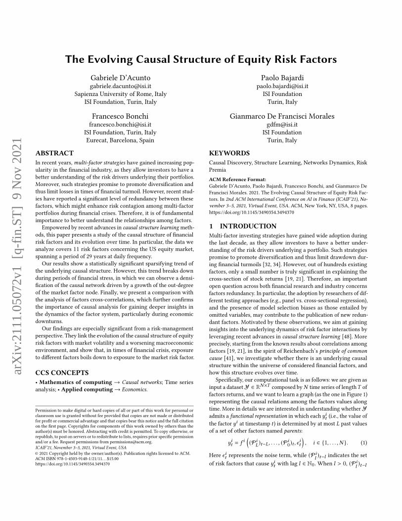
Specifically, our computational task is as follows: we are given asinput a datasetY ∈ R𝑁×𝑇 composed by𝑁 time series of length𝑇 offactors returns, and we want to learn a graph (as the one in Figure 1)representing the causal relations among the factors values alongtime. More in details we are interested in understanding whetherYadmits a functional representation in which each 𝑦𝑖𝑡 (i.e., the value ofthe factor 𝑦𝑖 at timestamp 𝑡 ) is determined by at most 𝐿 past valuesof a set of other factors named parents:

𝑦𝑖𝑡 = 𝑓 𝑖((P𝑖

𝐿)𝑡−𝐿, . . . , (P𝑖0)𝑡 , 𝜖

𝑖𝑡

), 𝑖 ∈ {1, . . . , 𝑁 }. (1)

Here 𝜖𝑖𝑡 represents the noise term, while (P𝑖𝑙)𝑡−𝑙 indicates the set

of risk factors that cause 𝑦𝑖𝑡 with lag 𝑙 ∈ N0. When 𝑙 > 0, (P𝑖𝑙)𝑡−𝑙

arX

iv:2

111.

0507

2v1

[q-

fin.

ST]

9 N

ov 2

021

ICAIF’21, November 3–5, 2021, Virtual Event, USA D’Acunto, et al.

Figure 1: An example of the causal graph among equity riskfactors along time with maximum lag 𝐿 = 2.

may contain 𝑦𝑖𝑡−𝑙 as well. Conversely, as we cannot observe causal

effects from present to past, (P𝑖0)𝑡 can neither contain 𝑦𝑖𝑡 nor 𝑦

𝑗𝑡 if

𝑦𝑖𝑡 ∈ (P 𝑗

0)𝑡 , otherwise it would be impossible to define the direc-tion of the causal relation. More in general, we require the set ofEquations (1) to be acyclic, which means that feedback loops amongvariables are forbidden. This assumption plays a key role in causalinference since it allows to set causes apart from effects.

In case the aforementioned functional forms are assumed to belinear, by using matrix notation, Equations (1) can be compactlywritten as a structural vector autoregressive model (SVAR)

y𝑡 =𝐿∑︁𝑙=0

W𝑙y𝑡−𝑙 + 𝝐𝑡 , (2)

where y𝑡 ∈ R𝑁 is a column vector constituted by the observationsat time 𝑡 ,W𝑙 ∈ R𝑁×𝑁 are the matrices of lagged causal effects withlag 𝑙 up to maximum lag 𝐿, such that𝑤𝑙

𝑖 𝑗≠ 0 iff 𝑦

𝑗

𝑡−𝑙 ∈ (P𝑖𝑙)𝑡−𝑙 . In

addition, the matrix of instantaneous causal effects W0 respectsthe acyclicity requirement mentioned above. Finally, 𝝐𝑡 ∈ R𝑁 isthe column vector of random disturbances at time 𝑡 .

We remark that Equation (2) should not be read as a usual sys-tem of equations, but rather as a set of functions describing howcertain factors determine others. Indeed, the model is said to bestructural since it allows to compute variables (effects) by means oflinear functions of other endogenous variables (causes), by takinginto account both instantaneous and lagged relations (also referredto as inter-layer connections). In particular, the previous modelcan be thought of as a combination of a structural equation model(SEM [38]) and a vector autoregressive model (VAR [46]).

Finally, note that Equation (2) entails a directed acyclic graph(DAG) in which there is a weighted edge from 𝑦

𝑗

𝑡−𝑙 ∈ (P𝑖𝑙)𝑡−𝑙 (with

𝑙 ≥ 0) to𝑦𝑖𝑡 : this is the causal graph of factors along time as depictedin Figure 1.

In order to study the evolution of such non-stationary system, weestimate Equation (2) by adopting a sliding window approach andperforming a regression analysis on the inferred causal networks.Our data covers 11 risk factors concerning the US equity market,over a period of 29 years at daily frequency. Our main results canbe summarized as follows:

• Causal interactions between factors exhibit a statistically sig-nificant sparsification trend along time, with anomalies inperiods of financial turmoil.

• We expose a relationship between the density of the causalnetworks and investor sentiment. In particular, we show thatperiods of worsening sentiment and business cycle phase (seeSection 3.2) are associated with a densification of the causalnetwork. This phenomenon is driven by a growth in the out-degree of the market risk factor.

• Finally, we conduct a comparative study between causationand correlation among factors. Our findings highlight howcausal analysis better describes the importance of the marketfactor among the considered risk factors. Besides, while ac-cording to correlation analysis, the business cycle indicator isnot related to the evolution of the factorial system, the study ofcausal structures reveals a statistically significant relationshipwith a 95% confidence level.

The rest of the paper is organized as follows. Section 2 providesthe background about factor investing and causal discovery. Sec-tion 3 describes the data used to conduct the analysis and presentsour methodology. Section 4 reports the results of our analysis. Fi-nally, Section 5, provides a discussion on our results together withsome direction for future investigation.

2 RELATEDWORKAn equity risk factor is a variable able to explain the cross-section ofexpected stock returns, i.e., how the expected return varies amongstocks. Its significance is usually assessed via the usage of linearregression models [12]. Factor investing is well rooted in finance, inparticular it dates back to the first asset pricing model, the CapitalAsset Pricing Model (CAPM), introduced by Sharpe [43]. CAPMlooks at stock returns through the exposure to one factor, the mar-ket beta, and introduces a precise definition of risk and how itdrives expected stock returns. Successively, Fama and French [17]found out that the exposure to small cap stocks (SMB) and cheaper,under-priced stocks (HML) provide two additional sources of risknot captured by CAPM. Based on these evidences, an enormousamount of research has been produced on factor investing, and hun-dreds of potential factors have been proposed [13, 22, 26, 35]. Thisabundance of proposed factors has opened an important questionacross both financial research and industry concerning their redun-dancy. As already mentioned, Feng et al. [19] and Harvey and Liu[21] recently pointed out that only a small number of the existingfactors is truly significant in explaining stock returns cross-section.Our study of risk factor interactions fits into this stream of research,and in particular tackles the problem by exploiting recent advancesin causal learning [37].

The possibility of examining a system under interventions (i.e.,counterfactual analysis) makes causal analysis a powerful tool forstudying complex systems [39]. However, in many cases, the under-lying causal structure is unknown, and it is not possible to carry outrandomized experiments in order to study the system at hand un-der distribution changes. Therefore, the interest in inferring causalstructures from observational data, also known as causal structurelearning, has been significantly growing during recent years.

Causal structure learning algorithms can be classified into threemain families: (i) constraint-based approaches, which make use ofconditional independence tests to establish the presence of an edgebetween two nodes [29, 47]; (ii) score-based methods, which use

The Evolving Causal Structure of Equity Risk Factors ICAIF’21, November 3–5, 2021, Virtual Event, USA

several search procedures in order to optimize a certain score func-tion [10, 23, 28]; (iii) structural causal models, which express a vari-able at a certain node as a function of its parents [8, 27, 40, 44, 45].Additionally, as highlighted in Section 1, whenever we are dealingwith a process that evolves over time, temporal ordering drivesthe causal inference procedure. Nevertheless, the main issue con-cerns the estimation of instantaneous effects, which must satisfythe acyclicity requirement. With regards to Equation (2), this meansthat W0 must entail the structure of a DAG.

However, it is common to deal with non-Gaussian data. Forinstance, this is the case of equity time series which show het-eroscedasticity (i.e., the variance of the stock returns varies overtime) and volatility clustering (i.e., large (small) swings in stockprices tend to group together) [6].

This observation implies that there is additional information, notdescribed by the covariance matrix, that can be exploited to retrieveW0. Consequently, by leveraging a non-gaussianity assumption of𝝐𝑡 , a series of linear non-Gaussian methods to estimate the modelin Equation (2) have been proposed in the past years [31, 36]. Inparticular, in this study we employ VAR-LiNGAM [31], as providedby the python package lingam1 made available by authors.

Econophysics, is an interdisciplinary effort devoted at analyzingthe risk contagion among financial institutions by representingthe financial system as a network [4], Our analysis differs fromEconophysics as we do not focus on financial institutions, andinstead aim to understand the dynamics of the factorial network,which captures sources of risk largely accepted and widely used byinvestors. In addition, we look for causal relationships between theobserved variables by means of a machine learning causal modelthat, differently from existing work [5], allows us to evaluate thepresence of instantaneous causal effects as well.

3 DATA AND METHODOLOGYIn this section, we first introduce the financial risk factors andprovide some information about the factor dataset Y. Then, wefocus on the additional variables selected as indicators of changes inboth investor expectation and business cycle evolution. Finally, wepresent the adopted causal inference approach and introduce thegeneralized linear model (GLM) regression we employ to analyzethe model results.

3.1 Financial factorsWe consider 11 risk factors at daily frequency concerning theUS equity market. The choice to use equity factors from the lat-ter market is driven by the greater availability of data and thehigher presence of results in the financial literature that can becompared to those we obtain. More precisely, we deal with 7306daily observations spanning 29 years, from 2 January 1991 to 31December 2019. We include in our analysis the following publishedrisk factors, gathered directly from the websites of authors: Ex-cess Market Return (Mkt-RF) [33], Small Minus Big (SMB) and HighMinus Low (HML) [17], Momentum (UMD) [9], HML Devil (HMLDev) [2], Robust Minus Weak (RMW) and Conservative Minus Ag-gressive (CMA) [18], HXZ Investment (R-IA) and HXZ Profitability

1https://github.com/cdt15/lingam

−4000 −2000 0 2000 4000Lag

0.0

0.2

0.4

0.6

0.8

Co

rrel

ati

on

valu

e

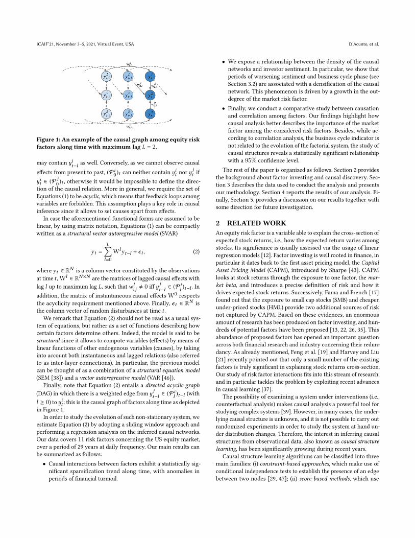
Figure 2: Cross-correlation function between CMA (Conser-vative Minus Aggressive) and R-IA (HXZ Investment).

(R-ROE) [25], Betting Against Beta (BAB) and Quality Minus Junk(QMJ) [3].

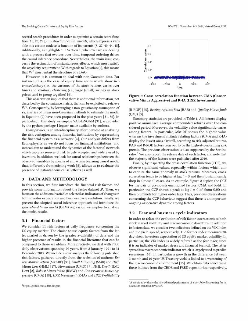
Summary statistics are provided in Table 1. All factors displaypositive annualised average compounded returns over the con-sidered period. Moreover, the volatility value significantly variesamong factors. In particular, Mkt-RF shows the highest valuewhereas the investment attitude relating factors (CMA and R-IA)display the lowest ones. Overall, according to risk-adjusted returns,BAB and R-ROE factors turn out to be the highest-performing riskpremia. The previous observation is also supported by the Sortinoratio.2 We also report the release date of each factor, and note thatthe majority of the factors were published after 2010.

Finally, by inspecting the cross-correlation function (CCF), weobserve significant values, especially within factors which aimto capture the same anomaly in stock returns. Moreover, cross-correlation tends to be higher at lag 𝑙 = 0 and then to significantlydrop in almost all cases. As an example, Figure 2 depicts the CCFfor the pair of previously-mentioned factors, CMA and R-IA. Inparticular, the CCF shows a peak at lag 𝑙 = 0 of about 0.90 andthen plummets for higher order lags. Thus, previous observationsconcerning the CCF behaviour suggest that there is an importantongoing associative dynamic among factors.

3.2 Fear and business cycle indicatorsIn order to relate the evolution of risk factor interactions to bothstock market volatility and macroeconomic downturn, in additionto factors data, we consider two indicators defined on the VIX Indexand the yield spread, respectively. The former index measures 30-day-ahead investors expectation of US equity market volatility. Inparticular, the VIX Index is widely referred as the fear index, sinceit is an indicator of market stress and financial turmoil. The latterspread is a macroeconomic indicator which is largely used to predictrecessions [16]. In particular a growth in the difference between3-month and 10-year US Treasury yield is linked to a worsening ofthe macroeconomic environment [15]. We obtain data concerningthese indexes from the CBOE and FRED repositories, respectively.

2A metric to evaluate the risk-adjusted performance of a portfolio discounting for itsdownside standard deviation.

ICAIF’21, November 3–5, 2021, Virtual Event, USA D’Acunto, et al.

Table 1: Summary statistics for the analyzed factors at daily frequency. Average compounded return, volatility, risk adjustedreturn, and Sortino Ratio are annualised.

Mkt-RF SMB HML RMW CMA R-IA R-ROE BAB HML-dev UMD QMJ

Avg Comp. Ret. (%) 7.68 0.67 2.10 3.89 2.14 2.23 5.35 9.43 0.65 5.17 4.46Volatility (%) 17.46 9.17 9.61 7.29 6.53 6.60 7.43 11.01 10.46 13.39 7.97Risk Adj. Ret. (%) 0.44 0.07 0.22 0.53 0.33 0.34 0.72 0.86 0.06 0.39 0.56Sortino Ratio (%) 0.62 0.10 0.32 0.79 0.47 0.48 1.04 1.21 0.09 0.53 0.83Skew -0.15 -0.22 0.43 0.26 -0.44 -0.72 -0.11 -0.34 0.52 -0.23 0.20Kurtosis 8.34 3.91 9.05 7.71 11.44 15.92 5.84 11.72 11.47 24.57 8.701st %-ile (%) -2.98 -1.46 -1.67 -1.28 -1.10 -1.08 -1.41 -2.20 -1.73 -2.52 -1.305th %-ile (%) -1.72 -0.91 -0.83 -0.66 -0.57 -0.57 -0.68 -0.97 -0.88 -1.20 -0.71Min -8.95 -4.71 -4.39 -3.02 -5.94 -6.88 -3.96 -6.29 -7.00 -9.46 -3.74Max 11.35 3.78 4.83 4.49 2.53 2.75 3.26 7.94 6.35 14.53 5.04

Publication year 1972 1993 1993 2015 2015 2014 2014 2014 2013 1997 2013

Starting from these two indexes, we build fear and business cyclez-scores as follows.We first define theΔVIX historical expected short-fall for the 𝑘-th inference sample period 𝑆𝑘 : ΔVIX-𝐸𝑆𝑘 = E[V95

𝑘],

defined over V95𝑘

= {𝑣𝑖 ∈ 𝑆𝑘 |𝑣𝑖 > 𝑣95𝑘

}, where 𝑣95𝑘

is the 95-percentile value of the percent change between VIX Index closingand opening daily values. By computing ΔVIX-𝐸𝑆𝑘 we quantifythe extreme values of the daily volatility swing over the inferenceperiod 𝑆𝑘 . Next, we measure the extent to which such a value isunusual with respect to past observations. Therefore, we define:

f-zscore =ΔVIX-𝐸𝑆𝑘 − `10𝑌

𝑘

𝜎10𝑌𝑘

with `10𝑌𝑘

and 𝜎10𝑌𝑘

being the 10-year rolling average and standarddeviation of ΔVIX-𝐸𝑆𝑘 respectively.

For the business cycle z-score, we first evaluate the extreme valuesof the 3M10Y yield spread for sample 𝑆𝑘 , i.e., 3M10Y-𝐸𝑆𝑘 = E[B95

𝑘],

defined over B95𝑘

= {𝑏𝑖 ∈ 𝑆𝑘 |𝑏𝑖 > 𝑏95𝑘

}, where, 𝑏95𝑘

is the 95-percentile value of the difference between the 3-month and 10-yearUS Treasury daily rates. Thus, we define the z-score as:

bc-zscore =Δ3M10Y-𝐸𝑆𝑘 − `10𝑌

𝑘

𝜎10𝑌𝑘

where `10𝑌𝑘

and 𝜎10𝑌𝑘

represent the 10-year rolling average andstandard deviation of Δ3M10Y-𝐸𝑆𝑘 respectively.

3.3 Causal inference procedure and regressionmodel

As mentioned earlier, to study the dynamic of the causal structurealong time, we adopt a sliding window approach. More precisely,we divide the overall analysis period into windows 𝑆𝑘 of length18 months each, with a sliding step of 3 months, obtaining 111inference periods 𝑆𝑘 .

As described in Section 2, we apply the VAR-LiNGAM algo-rithm to infer the causal model. In particular, the algorithm firstfits a VAR model on the data, and then estimates on the regressionresiduals a linear non-Gaussian causal inference method, the Di-rectLiNGAM [45]. Other existing linear non-Gaussian approachesleverage independent component analysis (ICA [30]) to estimate

the matrix of instantaneous causal effectW0. The DirectLiNGAMmodel was proposed to solve the potential convergence issues ofICA-based methods [24]. After the fit of VAR model on data, sup-pose to regress the residuals associated with factor 𝑗 on those offactor 𝑖 , ∀𝑗 ∈ {1, . . . , 𝑁 } | 𝑗 ≠ 𝑖 . Then, the residual 𝑧𝑖 is exoge-neous to the system if it is independent of the regression residual𝑟 𝑖𝑗= 𝑧 𝑗 − (𝑐𝑜𝑣 (𝑧 𝑗 , 𝑧𝑖 )/𝑣𝑎𝑟 (𝑧𝑖 ))𝑧𝑖 . The algorithm starts with an

empty causal ordering set O and, iteratively, appends the variablewhich is the most independent of its residual. The procedure stopswhen 𝑁 − 1 insertions have been made.

In each sample period, we apply the model by selecting thenumber of lags according to the BIC criterion [42]: the resultingmaximum lag 𝐿 is equal to 1 for every sample. Subsequently, wevalidate the estimated causal coefficients by running a permutationtest, i.e., resampling with replacement, with a significance levelequal to 95%. In addition, the total number of permuted samples perperiod is 5000, the length of the generated samples equals that of theinference period (18 months) and we do not apply any thresholdingto the resulting significant coefficients. Since we are interested incomparing the information provided by causal inference with thatcoming from correlation analysis, the same methodology is usedto estimate correlation networks, by replacing the estimation ofEquation (2) with the Pearson correlation coefficient.

Once we retrieve both causal and correlation network structures,we analyse their temporal evolution by means of a regression anal-ysis. We set as dependent variable 𝑑 the number of network edgesand as covariates the following three variables: time (measured indays), f-zscore, and bc-zscore. Moreover, since 𝑑 ∈ N0, we employa Poisson log-linear model specified by the following GLM [1]:

𝑙𝑜𝑔(𝑑) = 𝛽0 +3∑︁

𝑖=1

𝛽𝑖 · 𝑓𝑖 , (3)

from which we have 𝑑 = 𝑒𝛽0 ·∏3𝑖=1 𝑒

𝛽𝑖 ·𝑓𝑖 , where 𝑓𝑖 are the regres-sors mentioned before. Therefore, according to Equation (3), a unitincrease in the independent variable 𝑓𝑖 is associated with a multi-plicative effect 𝑒𝛽𝑖 on 𝑑 . As a consequence, if 𝛽𝑖 = 0, the growth of𝑓𝑖 does not affect that of 𝑑 . Furthermore, if 𝛽𝑖 > 0 then 𝑑 increasesas 𝑓𝑖 grows, and conversely if 𝛽𝑖 < 0 it decreases.

The Evolving Causal Structure of Equity Risk Factors ICAIF’21, November 3–5, 2021, Virtual Event, USA

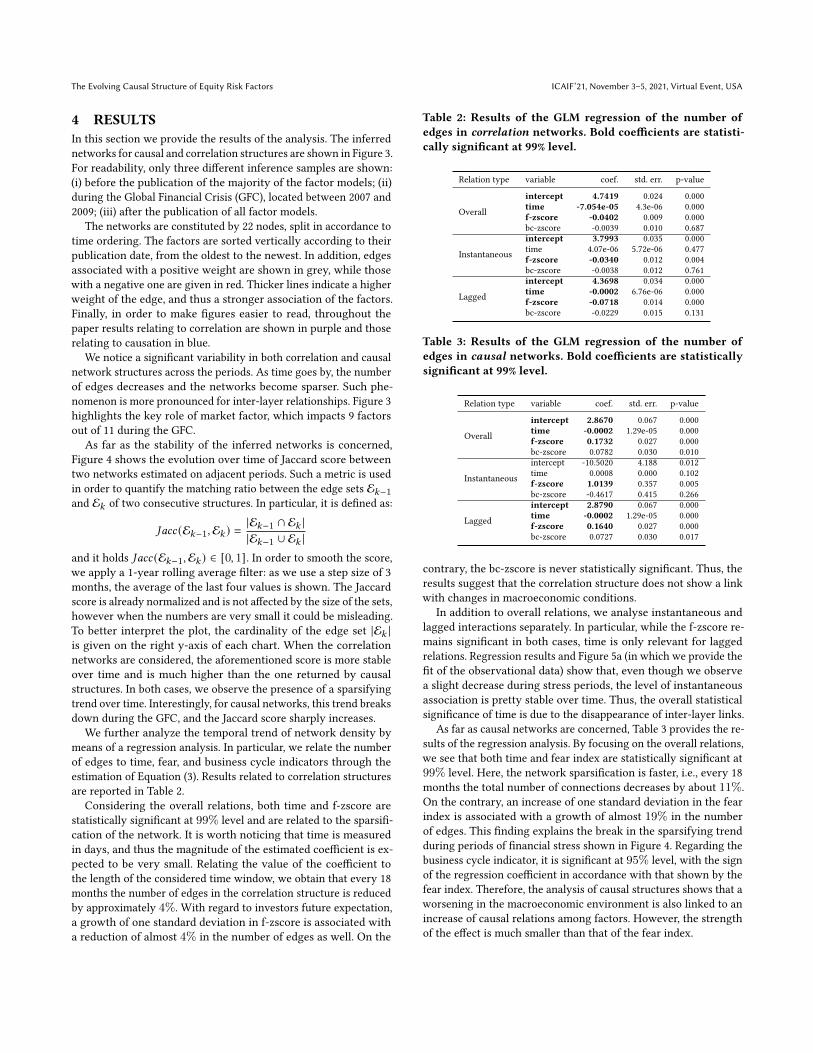
4 RESULTSIn this section we provide the results of the analysis. The inferrednetworks for causal and correlation structures are shown in Figure 3.For readability, only three different inference samples are shown:(i) before the publication of the majority of the factor models; (ii)during the Global Financial Crisis (GFC), located between 2007 and2009; (iii) after the publication of all factor models.

The networks are constituted by 22 nodes, split in accordance totime ordering. The factors are sorted vertically according to theirpublication date, from the oldest to the newest. In addition, edgesassociated with a positive weight are shown in grey, while thosewith a negative one are given in red. Thicker lines indicate a higherweight of the edge, and thus a stronger association of the factors.Finally, in order to make figures easier to read, throughout thepaper results relating to correlation are shown in purple and thoserelating to causation in blue.

We notice a significant variability in both correlation and causalnetwork structures across the periods. As time goes by, the numberof edges decreases and the networks become sparser. Such phe-nomenon is more pronounced for inter-layer relationships. Figure 3highlights the key role of market factor, which impacts 9 factorsout of 11 during the GFC.

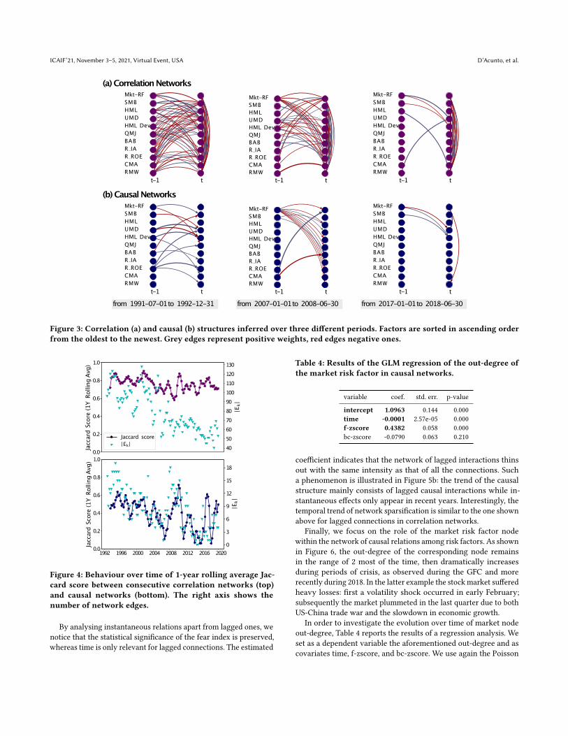
As far as the stability of the inferred networks is concerned,Figure 4 shows the evolution over time of Jaccard score betweentwo networks estimated on adjacent periods. Such a metric is usedin order to quantify the matching ratio between the edge sets E𝑘−1and E𝑘 of two consecutive structures. In particular, it is defined as:

𝐽𝑎𝑐𝑐 (E𝑘−1, E𝑘 ) =|E𝑘−1 ∩ E𝑘 ||E𝑘−1 ∪ E𝑘 |

and it holds 𝐽𝑎𝑐𝑐 (E𝑘−1, E𝑘 ) ∈ [0, 1]. In order to smooth the score,we apply a 1-year rolling average filter: as we use a step size of 3months, the average of the last four values is shown. The Jaccardscore is already normalized and is not affected by the size of the sets,however when the numbers are very small it could be misleading.To better interpret the plot, the cardinality of the edge set |E𝑘 |is given on the right y-axis of each chart. When the correlationnetworks are considered, the aforementioned score is more stableover time and is much higher than the one returned by causalstructures. In both cases, we observe the presence of a sparsifyingtrend over time. Interestingly, for causal networks, this trend breaksdown during the GFC, and the Jaccard score sharply increases.

We further analyze the temporal trend of network density bymeans of a regression analysis. In particular, we relate the numberof edges to time, fear, and business cycle indicators through theestimation of Equation (3). Results related to correlation structuresare reported in Table 2.

Considering the overall relations, both time and f-zscore arestatistically significant at 99% level and are related to the sparsifi-cation of the network. It is worth noticing that time is measuredin days, and thus the magnitude of the estimated coefficient is ex-pected to be very small. Relating the value of the coefficient tothe length of the considered time window, we obtain that every 18months the number of edges in the correlation structure is reducedby approximately 4%. With regard to investors future expectation,a growth of one standard deviation in f-zscore is associated witha reduction of almost 4% in the number of edges as well. On the

Table 2: Results of the GLM regression of the number ofedges in correlation networks. Bold coefficients are statisti-cally significant at 99% level.

Relation type variable coef. std. err. p-value

Overallintercept 4.7419 0.024 0.000time -7.054e-05 4.3e-06 0.000f-zscore -0.0402 0.009 0.000bc-zscore -0.0039 0.010 0.687

Instantaneousintercept 3.7993 0.035 0.000time 4.07e-06 5.72e-06 0.477f-zscore -0.0340 0.012 0.004bc-zscore -0.0038 0.012 0.761

Laggedintercept 4.3698 0.034 0.000time -0.0002 6.76e-06 0.000f-zscore -0.0718 0.014 0.000bc-zscore -0.0229 0.015 0.131

Table 3: Results of the GLM regression of the number ofedges in causal networks. Bold coefficients are statisticallysignificant at 99% level.

Relation type variable coef. std. err. p-value

Overallintercept 2.8670 0.067 0.000time -0.0002 1.29e-05 0.000f-zscore 0.1732 0.027 0.000bc-zscore 0.0782 0.030 0.010

Instantaneousintercept -10.5020 4.188 0.012time 0.0008 0.000 0.102f-zscore 1.0139 0.357 0.005bc-zscore -0.4617 0.415 0.266

Laggedintercept 2.8790 0.067 0.000time -0.0002 1.29e-05 0.000f-zscore 0.1640 0.027 0.000bc-zscore 0.0727 0.030 0.017

contrary, the bc-zscore is never statistically significant. Thus, theresults suggest that the correlation structure does not show a linkwith changes in macroeconomic conditions.

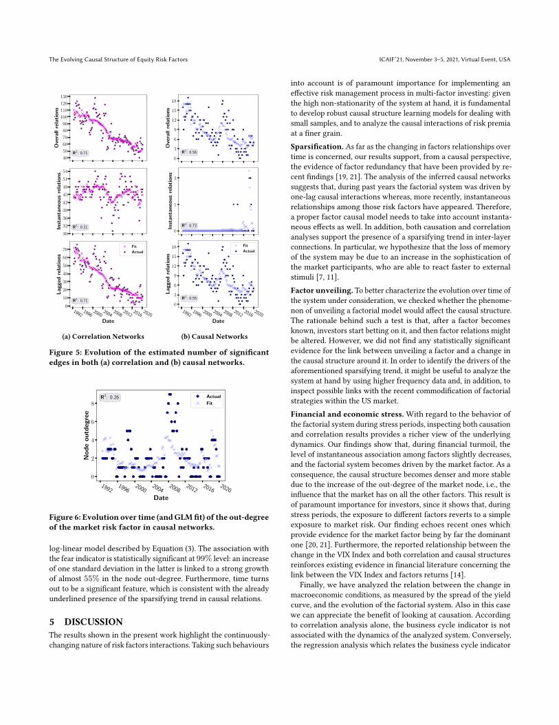
In addition to overall relations, we analyse instantaneous andlagged interactions separately. In particular, while the f-zscore re-mains significant in both cases, time is only relevant for laggedrelations. Regression results and Figure 5a (in which we provide thefit of the observational data) show that, even though we observea slight decrease during stress periods, the level of instantaneousassociation is pretty stable over time. Thus, the overall statisticalsignificance of time is due to the disappearance of inter-layer links.

As far as causal networks are concerned, Table 3 provides the re-sults of the regression analysis. By focusing on the overall relations,we see that both time and fear index are statistically significant at99% level. Here, the network sparsification is faster, i.e., every 18months the total number of connections decreases by about 11%.On the contrary, an increase of one standard deviation in the fearindex is associated with a growth of almost 19% in the numberof edges. This finding explains the break in the sparsifying trendduring periods of financial stress shown in Figure 4. Regarding thebusiness cycle indicator, it is significant at 95% level, with the signof the regression coefficient in accordance with that shown by thefear index. Therefore, the analysis of causal structures shows that aworsening in the macroeconomic environment is also linked to anincrease of causal relations among factors. However, the strengthof the effect is much smaller than that of the fear index.

ICAIF’21, November 3–5, 2021, Virtual Event, USA D’Acunto, et al.

Mkt-RFSMBHMLUMDHML DevQMJBABR IAR ROECMARMW

t-1 t

Mkt-RFSMBHMLUMDHML DevQMJBABR IAR ROECMARMW

t-1 t

Mkt-RFSMBHMLUMDHML DevQMJBABR IAR ROECMARMW

t-1 t

Mkt-RFSMBHMLUMDHML DevQMJBABR IAR ROECMARMW

t-1 t

Mkt-RFSMBHMLUMDHML DevQMJBABR IAR ROECMARMW

t-1 t

Mkt-RFSMBHMLUMDHML DevQMJBABR IAR ROECMARMW

t-1 t

(a)CorrelationNetworks

(b)CausalNetworks

from 1991-07-01to 1992-12-31 from 2007-01-01to 2008-06-30 from 2017-01-01to 2018-06-30

Figure 3: Correlation (a) and causal (b) structures inferred over three different periods. Factors are sorted in ascending orderfrom the oldest to the newest. Grey edges represent positive weights, red edges negative ones.

1992 1996 2000 2004 2008 2012 2016 20200.0

0.2

0.4

0.6

0.8

1.0

JaccardScore(1YRolling

Avg)

0

3

6

9

12

15

18

|Ek|

0.0

0.2

0.4

0.6

0.8

1.0

JaccardScore(1YRolling

Avg)

405060708090100110120130

|Ek|

Jaccard score|Ek|

Figure 4: Behaviour over time of 1-year rolling average Jac-card score between consecutive correlation networks (top)and causal networks (bottom). The right axis shows thenumber of network edges.

By analysing instantaneous relations apart from lagged ones, wenotice that the statistical significance of the fear index is preserved,whereas time is only relevant for lagged connections. The estimated

Table 4: Results of the GLM regression of the out-degree ofthe market risk factor in causal networks.

variable coef. std. err. p-value

intercept 1.0963 0.144 0.000time -0.0001 2.57e-05 0.000f-zscore 0.4382 0.058 0.000bc-zscore -0.0790 0.063 0.210

coefficient indicates that the network of lagged interactions thinsout with the same intensity as that of all the connections. Sucha phenomenon is illustrated in Figure 5b: the trend of the causalstructure mainly consists of lagged causal interactions while in-stantaneous effects only appear in recent years. Interestingly, thetemporal trend of network sparsification is similar to the one shownabove for lagged connections in correlation networks.

Finally, we focus on the role of the market risk factor nodewithin the network of causal relations among risk factors. As shownin Figure 6, the out-degree of the corresponding node remainsin the range of 2 most of the time, then dramatically increasesduring periods of crisis, as observed during the GFC and morerecently during 2018. In the latter example the stockmarket sufferedheavy losses: first a volatility shock occurred in early February;subsequently the market plummeted in the last quarter due to bothUS-China trade war and the slowdown in economic growth.

In order to investigate the evolution over time of market nodeout-degree, Table 4 reports the results of a regression analysis. Weset as a dependent variable the aforementioned out-degree and ascovariates time, f-zscore, and bc-zscore. We use again the Poisson

The Evolving Causal Structure of Equity Risk Factors ICAIF’21, November 3–5, 2021, Virtual Event, USA

40

50

60

70

80

90

100

110

120

130

Ove

rall

rela

tio

ns

R2: 0.71

30

33

36

39

42

45

48

51

54

Inst

an

tan

eou

sre

lati

on

s

R2: 0.21

19921996

20002004

20082012

20162020

Date

0

10

20

30

40

50

60

70

La

gg

edre

lati

on

s

R2: 0.71

Fit

Actual

(a) Correlation Networks

0

3

6

9

12

15

18

Ove

rall

rela

tio

ns

R2: 0.56

0

1

2

Inst

an

tan

eou

sre

lati

on

s

R2: 0.73

19921996

20002004

20082012

20162020

Date

0

3

6

9

12

15

18

La

gg

edre

lati

on

s

R2: 0.55

Fit

Actual

(b) Causal Networks

Figure 5: Evolution of the estimated number of significantedges in both (a) correlation and (b) causal networks.

19921996

20002004

20082012

20162020

Date

0

2

4

6

8

No

de

ou

tdeg

ree

R2: 0.26 Actual

Fit

Figure 6: Evolution over time (andGLMfit) of the out-degreeof the market risk factor in causal networks.

log-linear model described by Equation (3). The association withthe fear indicator is statistically significant at 99% level: an increaseof one standard deviation in the latter is linked to a strong growthof almost 55% in the node out-degree. Furthermore, time turnsout to be a significant feature, which is consistent with the alreadyunderlined presence of the sparsifying trend in causal relations.

5 DISCUSSIONThe results shown in the present work highlight the continuously-changing nature of risk factors interactions. Taking such behaviours

into account is of paramount importance for implementing aneffective risk management process in multi-factor investing: giventhe high non-stationarity of the system at hand, it is fundamentalto develop robust causal structure learning models for dealing withsmall samples, and to analyze the causal interactions of risk premiaat a finer grain.Sparsification. As far as the changing in factors relationships overtime is concerned, our results support, from a causal perspective,the evidence of factor redundancy that have been provided by re-cent findings [19, 21]. The analysis of the inferred causal networkssuggests that, during past years the factorial system was driven byone-lag causal interactions whereas, more recently, instantaneousrelationships among those risk factors have appeared. Therefore,a proper factor causal model needs to take into account instanta-neous effects as well. In addition, both causation and correlationanalyses support the presence of a sparsifying trend in inter-layerconnections. In particular, we hypothesize that the loss of memoryof the system may be due to an increase in the sophistication ofthe market participants, who are able to react faster to externalstimuli [7, 11].Factor unveiling. To better characterize the evolution over time ofthe system under consideration, we checked whether the phenome-non of unveiling a factorial model would affect the causal structure.The rationale behind such a test is that, after a factor becomesknown, investors start betting on it, and then factor relations mightbe altered. However, we did not find any statistically significantevidence for the link between unveiling a factor and a change inthe causal structure around it. In order to identify the drivers of theaforementioned sparsifying trend, it might be useful to analyze thesystem at hand by using higher frequency data and, in addition, toinspect possible links with the recent commodification of factorialstrategies within the US market.Financial and economic stress. With regard to the behavior ofthe factorial system during stress periods, inspecting both causationand correlation results provides a richer view of the underlyingdynamics. Our findings show that, during financial turmoil, thelevel of instantaneous association among factors slightly decreases,and the factorial system becomes driven by the market factor. As aconsequence, the causal structure becomes denser and more stabledue to the increase of the out-degree of the market node, i.e., theinfluence that the market has on all the other factors. This result isof paramount importance for investors, since it shows that, duringstress periods, the exposure to different factors reverts to a simpleexposure to market risk. Our finding echoes recent ones whichprovide evidence for the market factor being by far the dominantone [20, 21]. Furthermore, the reported relationship between thechange in the VIX Index and both correlation and causal structuresreinforces existing evidence in financial literature concerning thelink between the VIX Index and factors returns [14].

Finally, we have analyzed the relation between the change inmacroeconomic conditions, as measured by the spread of the yieldcurve, and the evolution of the factorial system. Also in this casewe can appreciate the benefit of looking at causation. Accordingto correlation analysis alone, the business cycle indicator is notassociated with the dynamics of the analyzed system. Conversely,the regression analysis which relates the business cycle indicator

ICAIF’21, November 3–5, 2021, Virtual Event, USA D’Acunto, et al.

to the causal structure of the factorial system displays a statisti-cally significant relationship with a 95% confidence level. Indeed,similarly to the results of the volatility analysis, the worsening ofmacroeconomic environment is associated with a growth in thenumber of network arcs. Therefore, looking at the causation al-lows to better inspect the evolution of the system during negativeeconomic phases.Future work. The results in this paper contribute to make someprogress in understanding the relationships among risk factors.However, several questions remain open. As an example, it wouldbe interesting to study the interactions among risk factors belong-ing to different equity markets. Moreover, our analysis concernsonly the equity asset class. Thus, enlarging the considered set offactors, by including risk premia concerning other asset classesas well, could help in taking into consideration also inter-assetclass dynamics. Finally, by construction, causal networks enablestudying the response of the system at hand under interventions.Therefore, it would be interesting to exploit the attained results tosetup a suitable stress testing procedure for multi-factor portfolios.

ACKNOWLEDGMENTSThe authors acknowledge the support from Intesa Sanpaolo Innova-tion Center. The funder had no role in study design, data collectionand analysis, decision to publish, or preparation of the manuscript.

REFERENCES[1] Alan Agresti. 2018. An introduction to categorical data analysis. John Wiley &

Sons. 74–90 pages.[2] Clifford Asness and Andrea Frazzini. 2013. The devil in HML’s details. The

Journal of Portfolio Management 39, 4 (2013), 49–68.[3] Clifford S Asness, Andrea Frazzini, and Lasse Heje Pedersen. 2019. Quality minus

junk. Review of Accounting Studies 24, 1 (2019), 34–112.[4] Marco Bardoscia, Paolo Barucca, Stefano Battiston, Fabio Caccioli, Giulio Cimini,

Diego Garlaschelli, Fabio Saracco, Tiziano Squartini, and Guido Caldarelli. 2021.The Physics of Financial Networks. arXiv preprint arXiv:2103.05623 (2021).

[5] Monica Billio, Mila Getmansky, AndrewW Lo, and Loriana Pelizzon. 2012. Econo-metric measures of connectedness and systemic risk in the finance and insurancesectors. Journal of financial economics 104, 3 (2012), 535–559.

[6] Tim Bollerslev. 1986. Generalized autoregressive conditional heteroskedasticity.Journal of econometrics 31, 3 (1986), 307–327.

[7] Jonathan Brogaard, Terrence Hendershott, and Ryan Riordan. 2014. High-frequency trading and price discovery. The Review of Financial Studies 27, 8(2014), 2267–2306.

[8] Peter Bühlmann, Jonas Peters, Jan Ernest, et al. 2014. CAM: Causal additivemodels, high-dimensional order search and penalized regression. Annals ofstatistics 42, 6 (2014), 2526–2556.

[9] Mark M Carhart. 1997. On persistence in mutual fund performance. The Journalof finance 52, 1 (1997), 57–82.

[10] David Maxwell Chickering. 2002. Optimal structure identification with greedysearch. Journal of machine learning research 3, Nov (2002), 507–554.

[11] Tarun Chordia, T Clifton Green, and Badrinath Kottimukkalur. 2018. Rent seekingby low-latency traders: Evidence from trading on macroeconomic announce-ments. The Review of Financial Studies 31, 12 (2018), 4650–4687.

[12] John H Cochrane. 2009. The Cross-section: CAPM and Multifactor Models. InAsset pricing (Revised edition). Princeton university press, Chapter 20, 435–449.

[13] John H Cochrane. 2011. Presidential address: Discount rates. The Journal offinance 66, 4 (2011), 1047–1108.

[14] Robert B Durand, Dominic Lim, and J Kenton Zumwalt. 2011. Fear and theFama-French factors. Financial Management 40, 2 (2011), 409–426.

[15] Arturo Estrella and Gikas A Hardouvelis. 1991. The term structure as a predictorof real economic activity. The journal of Finance 46, 2 (1991), 555–576.

[16] Arturo Estrella and Frederic S Mishkin. 1996. The yield curve as a predictor ofUS recessions. Current issues in economics and finance 2, 7 (1996).

[17] Eugene F Fama and Kenneth R French. 1993. Common risk factors in the returnson stocks and bonds. Journal of financial economics 33, 1 (1993), 3–56.

[18] Eugene F Fama and Kenneth R French. 2015. A five-factor asset pricing model.Journal of financial economics 116, 1 (2015), 1–22.

[19] Guanhao Feng, Stefano Giglio, and Dacheng Xiu. 2020. Taming the factor zoo: Atest of new factors. The Journal of Finance 75, 3 (2020), 1327–1370.

[20] Stefano Giglio and Dacheng Xiu. 2017. Inference on risk premia in the presence ofomitted factors. Technical Report. National Bureau of Economic Research.

[21] Campbell R. Harvey and Yan Liu. 2021. Lucky factors. Journal of FinancialEconomics (2021). https://doi.org/10.1016/j.jfineco.2021.04.014

[22] Campbell R Harvey, Yan Liu, and Heqing Zhu. 2015. . . . and the cross-section ofexpected returns. The Review of Financial Studies 29, 1 (2015), 5–68.

[23] David Heckerman, Dan Geiger, and David M Chickering. 1995. Learning Bayesiannetworks: The combination of knowledge and statistical data. Machine learning20, 3 (1995), 197–243.

[24] Johan Himberg, Aapo Hyvärinen, and Fabrizio Esposito. 2004. Validating the inde-pendent components of neuroimaging time series via clustering and visualization.Neuroimage 22, 3 (2004), 1214–1222.

[25] Kewei Hou, Chen Xue, and Lu Zhang. 2015. Digesting anomalies: An investmentapproach. The Review of Financial Studies 28, 3 (2015), 650–705.

[26] Kewei Hou, Chen Xue, and Lu Zhang. 2017. Replicating Anomalies. TechnicalReport. National Bureau of Economic Research.

[27] Patrik Hoyer, Dominik Janzing, Joris M Mooij, Jonas Peters, and BernhardSchölkopf. 2008. Nonlinear causal discovery with additive noise models. Advancesin neural information processing systems 21 (2008), 689–696.

[28] Biwei Huang, Kun Zhang, Yizhu Lin, Bernhard Schölkopf, and Clark Glymour.2018. Generalized score functions for causal discovery. In Proceedings of the 24thACM SIGKDD International Conference on Knowledge Discovery & Data Mining.1551–1560.

[29] Biwei Huang, Kun Zhang, Jiji Zhang, Joseph Ramsey, Ruben Sanchez-Romero,Clark Glymour, and Bernhard Schölkopf. 2020. Causal discovery from heteroge-neous/nonstationary data. Journal of Machine Learning Research 21, 89 (2020),1–53.

[30] Aapo Hyvarinen. 1999. Fast and robust fixed-point algorithms for independentcomponent analysis. IEEE transactions on Neural Networks 10, 3 (1999), 626–634.

[31] Aapo Hyvärinen, Kun Zhang, Shohei Shimizu, and Patrik O Hoyer. 2010. Estima-tion of a structural vector autoregression model using non-gaussianity. Journalof Machine Learning Research 11, 5 (2010).

[32] Antti Ilmanen and Jared Kizer. 2012. The Death of Diversification Has BeenGreatlyExaggerated. The Journal of Portfolio Management 38, 3 (2012), 15–27.

[33] Michael C Jensen, Fischer Black, and Myron S Scholes. 1972. The capital assetpricing model: Some empirical tests. In Studies in the Theory of Capital Markets.Praeger Publishers Inc.

[34] Philipp J Kremer, Andreea Talmaciu, and Sandra Paterlini. 2018. Risk minimiza-tion in multi-factor portfolios: What is the best strategy? Annals of OperationsResearch 266, 1 (2018), 255–291.

[35] R David McLean and Jeffrey Pontiff. 2016. Does academic research destroy stockreturn predictability? The Journal of Finance 71, 1 (2016), 5–32.

[36] Alessio Moneta, Doris Entner, Patrik O Hoyer, and Alex Coad. 2013. Causalinference by independent component analysis: Theory and applications. OxfordBulletin of Economics and Statistics 75, 5 (2013), 705–730.

[37] Judea Pearl. 2009. Causality. Cambridge university press.[38] Jonas Peters, Dominik Janzing, and Bernhard Schlkopf. 2017. Elements of Causal

Inference: Foundations and Learning Algorithms. The MIT Press. 33–41 pages.[39] Jonas Peters, Dominik Janzing, and Bernhard Schlkopf. 2017. Elements of Causal

Inference: Foundations and Learning Algorithms. The MIT Press. 1–14 pages.[40] Jonas Peters, Joris M Mooij, Dominik Janzing, and Bernhard Schölkopf. 2014.

Causal discovery with continuous additive noise models. Journal of MachineLearning Research (2014).

[41] Hans Reichenbach. 1956. The Direction of Time. University of California Press.[42] Gideon Schwarz et al. 1978. Estimating the dimension of a model. Annals of

statistics 6, 2 (1978), 461–464.[43] William F Sharpe. 1964. Capital asset prices: A theory of market equilibrium

under conditions of risk. The journal of finance 19, 3 (1964), 425–442.[44] Shohei Shimizu, Patrik O. Hoyer, Aapo Hyvärinen, and Antti Kerminen. 2006. A

Linear Non-Gaussian Acyclic Model for Causal Discovery. J. Mach. Learn. Res. 7(Dec. 2006), 2003–2030.

[45] Shohei Shimizu, Takanori Inazumi, Yasuhiro Sogawa, Aapo Hyvärinen, Yoshi-nobu Kawahara, Takashi Washio, Patrik O Hoyer, and Kenneth Bollen. 2011.DirectLiNGAM: A direct method for learning a linear non-Gaussian structuralequation model. The Journal of Machine Learning Research 12 (2011), 1225–1248.

[46] Christopher A Sims. 1980. Macroeconomics and reality. Econometrica: journal ofthe Econometric Society (1980), 1–48.

[47] Peter Spirtes, Clark N Glymour, Richard Scheines, and David Heckerman. 2000.Causation, prediction, and search. MIT press.

[48] Matthew J Vowels, Necati Cihan Camgoz, and Richard Bowden. 2021. D’ya likeDAGs? A Survey on Structure Learning and Causal Discovery. arXiv preprintarXiv:2103.02582 (2021).