Embed Size (px)
Citation preview
FACTA UNIVERSITATIS (NIS)
SER.: ELEC. ENERG. vol. 24, no. 3, December 2011, 451-482
The EXOR Gate Under Uncertainty: A Case Study
Svetlana N. Yanushkevich, An Hong Tran, Golam Tangim,Vladimir P. Shmerko, Elena N. Zaitseva and Vitaly Levashenko
Abstract: Probabilistic AND/EXOR networks have been defined, in the past, as aclass of Reed-Muller circuits, which operate on random signals. In contemporarylogic network design, it is classified asbehavioral notation of probabilistic logicgates and networks. In this paper, we introduce additional notations of probabilis-tic AND/EXOR networks:belief propagation, stochastic, decision diagram, neuro-morphicmodels, andMarkov random fieldmodel. Probabilistic logic networks, and,in particular, probabilistic AND/EXOR networks, known as turbo-decoders (used incell phones and iPhone) are in demand in the coding theory. Another example is in-telligent decision support in banking and security applications. We argue that thereare two types of probabilistic networks: traditional logicnetworks assuming randomsignals, andbelief propagationnetworks. We propose the taxonomy for this design,and provide the results of experimental study. In addition,we show that in forth-coming technologies, in particular, molecular electronics, probabilistic computing isthe platform for developing the devices and systems for low-power low-precise dataprocessing.
Keywords: AND-EXOR networks; probabilistic computation; belief propagationnetwork; decision diagram; neuromorphic network; Markov random field.
1 Introduction
The elementary Boolean function EXOR (Fig. 1) is notable in logic design becauseit is a basic operation of Reed-Muller techniques (an arbitrary Boolean function can
Manuscript received July 3, 2011. An earlier version of this paper was presented at the ReedMuller 2011 Workshop, May 25-26, 2011, Gustavelund Conference Centre, Tuusula, Finland.
S. N. Yanushkevich, A. H. Tran, G. Tangim, and V. P. Shmerko are with the De-partment of Electrical and Computer Engineering, University of Calgary, Canada, (e-mail:[email protected]). E. N. Zaitseva and V. Levashenko are with the Department of In-formatics, University of Zilina, Slovakia, (e-mail:[email protected]).
Digital Object Identifier: 10.2298/FUEE1103451Y
451

452 S. N. Yanushkevich et al.:
be implemented using EXOR and AND operations, and constant “1”) [29]. It is alsothe most often operation used in testing, coding techniques, and encryption[25].
Various fault-tolerant techniques for Reed-Muller have been proposed recently,in particular, [21]. However they cannot solve the problems, related to ran-dom intrinsic noise, which is observed in ultra deep submicron and predictablenanoscale devices. Moreover, there are various physical and chemical phenomenain nanospace, which can be directly encoded as EXOR function [22]. A three-dimensional implementation of EXOR functions has been proposed in [23].
Two-input EXOR gate (Nonequivalence)
Truth table Denotation Implementationx1 x2 f0 0 00 1 11 0 11 1 0
x1
x2
f
x1
x2 f
Two-input XNOR gate (Equivalence)
Truth table Denotation Implementation
x1 x2 f0 0 10 1 01 0 01 1 1
x1 x2
f
x1
x2 f
Fig. 1. Specification of two input EXOR gatef = x1⊕ x2, and XNOR gatef = x1⊕x2, givendeterministic inputs: the truth table, graphical denotation, and AND/OR implementation.
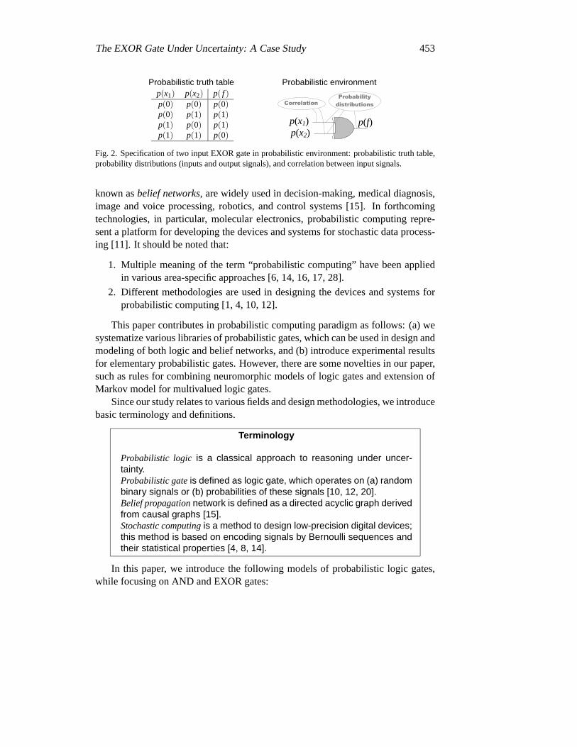
The deterministic model of EXOR gate (Fig. 1) operates on noise-free signals.Focus of this paper is the behavior of EXOR function in probabilistic environment,which is defined by replacing deterministic signals whith random signals. Specif-ically, when noise is allowed, input signals are applied to EXOR gate with somelevel of probability. Probabilistic models assume, that correct output signals arecalculated with some level of probability. Behavior of EXOR gate in probabilisticenvironment is completely described by probability distribution functions. Inputprobabilities are derived from these functions in the form of probabilistic truth ta-ble (Fig. 2). For simplification, it is also often assumed that the input signals areuncorrelated and independent. This problem in more general meaning is known asprobabilistic computation.
There are various fields, where probabilistic computing is the key technique.For example, in communication, the best error correcting technique, knownas turbocoding, is based on probabilistic data processing [1]. The devices and systems,
The EXOR Gate Under Uncertainty: A Case Study 453
Probabilistic truth table Probabilistic environmentp(x1) p(x2) p( f )p(0) p(0) p(0)p(0) p(1) p(1)p(1) p(0) p(1)p(1) p(1) p(0)
p(x1) p(x2)
p(f)
Correlation Probability
distributions
Fig. 2. Specification of two input EXOR gate in probabilistic environment: probabilistic truth table,probability distributions (inputs and output signals), and correlation between input signals.
known asbelief networks, are widely used in decision-making, medical diagnosis,image and voice processing, robotics, and control systems [15]. In forthcomingtechnologies, in particular, molecular electronics, probabilistic computing repre-sent a platform for developing the devices and systems for stochastic dataprocess-ing [11]. It should be noted that:
1. Multiple meaning of the term “probabilistic computing” have been appliedin various area-specific approaches [6, 14, 16, 17, 28].
2. Different methodologies are used in designing the devices and systems forprobabilistic computing [1, 4, 10, 12].
This paper contributes in probabilistic computing paradigm as follows: (a) wesystematize various libraries of probabilistic gates, which can be used in design andmodeling of both logic and belief networks, and (b) introduce experimental resultsfor elementary probabilistic gates. However, there are some novelties in ourpaper,such as rules for combining neuromorphic models of logic gates and extension ofMarkov model for multivalued logic gates.
Since our study relates to various fields and design methodologies, we introducebasic terminology and definitions.
Terminology
Probabilistic logic is a classical approach to reasoning under uncer-tainty.Probabilistic gateis defined as logic gate, which operates on (a) randombinary signals or (b) probabilities of these signals [10, 12, 20].Belief propagationnetwork is defined as a directed acyclic graph derivedfrom causal graphs [15].Stochastic computingis a method to design low-precision digital devices;this method is based on encoding signals by Bernoulli sequences andtheir statistical properties [4, 8, 14].
In this paper, we introduce the following models of probabilistic logic gates,while focusing on AND and EXOR gates:
454 S. N. Yanushkevich et al.:
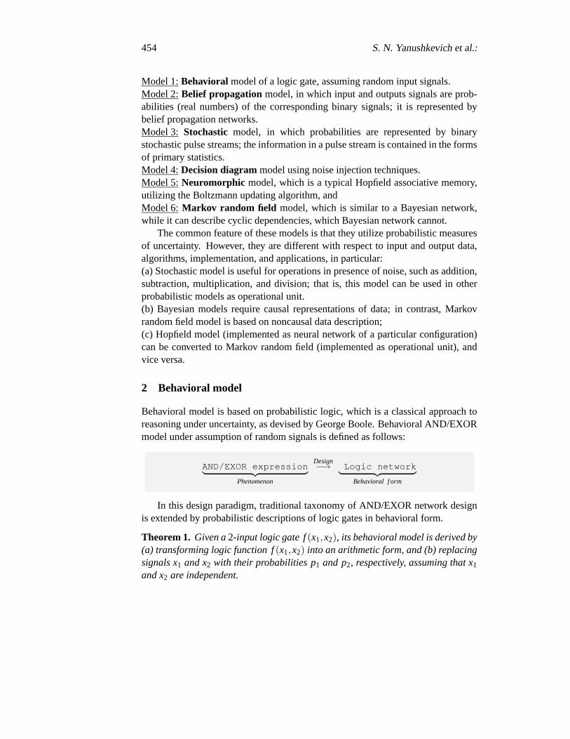
Model 1:Behavioral model of a logic gate, assuming random input signals.Model 2:Belief propagation model, in which input and outputs signals are prob-abilities (real numbers) of the corresponding binary signals; it is represented bybelief propagation networks.Model 3: Stochastic model, in which probabilities are represented by binarystochastic pulse streams; the information in a pulse stream is contained in the formsof primary statistics.Model 4:Decision diagrammodel using noise injection techniques.Model 5:Neuromorphic model, which is a typical Hopfield associative memory,utilizing the Boltzmann updating algorithm, andModel 6: Markov random field model, which is similar to a Bayesian network,while it can describe cyclic dependencies, which Bayesian network cannot.
The common feature of these models is that they utilize probabilistic measuresof uncertainty. However, they are different with respect to input and output data,algorithms, implementation, and applications, in particular:(a) Stochastic model is useful for operations in presence of noise, such as addition,subtraction, multiplication, and division; that is, this model can be used in otherprobabilistic models as operational unit.(b) Bayesian models require causal representations of data; in contrast, Markovrandom field model is based on noncausal data description;(c) Hopfield model (implemented as neural network of a particular configuration)can be converted to Markov random field (implemented as operational unit),andvice versa.
2 Behavioral model
Behavioral model is based on probabilistic logic, which is a classical approach toreasoning under uncertainty, as devised by George Boole. Behavioral AND/EXORmodel under assumption of random signals is defined as follows:
AND/EXOR expression︸ ︷︷ ︸
Phenomenon
Design−→ Logic network
︸ ︷︷ ︸
Behavioral f orm
In this design paradigm, traditional taxonomy of AND/EXOR network designis extended by probabilistic descriptions of logic gates in behavioral form.
Theorem 1. Given a2-input logic gate f(x1,x2), its behavioral model is derived by(a) transforming logic function f(x1,x2) into an arithmetic form, and (b) replacingsignals x1 and x2 with their probabilities p1 and p2, respectively, assuming that x1
and x2 are independent.

The EXOR Gate Under Uncertainty: A Case Study 455
Note that in behavioral model,p1 andp2 are the probabilities of signalsx1 andx2 being logic “1”, respectively. Proof of this theorem follows from the propertiesof probabilities for independent random events and the properties of arithmeticforms of Boolean functions.
Example 1. Let the inputs x1 and x2 of the 2-input EXOR gate be mutually inde-pendent with probabilities of being “1” p1 and p2, respectively. The behavioralmodel represents the probability of the output being logic “1” and is derived fromthe truth table of EXOR function:
p = (1− p1)p2︸ ︷︷ ︸
For x1 = 0,x2 = 1
+ p1(1− p2)︸ ︷︷ ︸
For x1 = 1,x2 = 0
= p1 + p2−2p1p2.
or by transforming the EXOR function into the arithmetic form, x1⊕ x2 = x1 +x2 + 2x1x2 and replacing xi with pi , i = 1,2, that is, p1 + p2−2p1p2. Supposingp1 = 0.8, p2 = 0.9, the logic “1” at the output is produced with probability p=0.8+0.9−2×0.8·0.9 = 0.26.
3 Belief propagation model
In the belief propagation model, any phenomenon must first be described incausalform, and then, using probabilistic relationships, transformed into a belief propa-gation network:
Phenomenon −→Causalmodel
︸ ︷︷ ︸
Propositions
Design−→
Beliefnetwork
︸ ︷︷ ︸
Computing
Causal modeling attempts to resolve question about possible causes so as toprovide explanation of phenomena (effects) as the result of previous phenomena(causes). Causal knowledge is modeled using the causal networks, in which thenodes represent propositions (or variables), the arcs signify directdependenciesbetween the linked propositions, and the strengths of these dependenciesare quan-tified by conditional probabilities. A Bayesian network is a type of belief networkthat captures the way the propositions relate to each other probabilistically.
The simplest form of the belief propagation model is as follows. Ifk eventsB1,B2, . . . ,Bk constitute a partition of the sample spaceS, such thatP(Bi) 6= 0 fori = 1,2, . . . ,k, then, for any eventsBr andA of Ssuch thatP(A) 6= 0,

456 S. N. Yanushkevich et al.:
P(Br |A)︸ ︷︷ ︸
Posterior
= P(A|Br)︸ ︷︷ ︸
Likelihood
×
Prior︷ ︸︸ ︷
P(Br)
P(A)︸︷︷︸
Evidence
wherer = 1,2, . . .k; P(Br |A) is a revisedor aposteriorprobability;P(A|Br) is thelikelihood of Br with respect toA; P(A) is theevidence factorand can be viewedas merely a scale factor, that guarantees that the posterior probabilities sum to one,as all good probabilities must.
This belief propagation form, or Bayesian principle, advises on how to updateprobabilities, once such a conditional probability structure has been adapted, givenappropriate prior probabilities.
Let the nodes of a graph represent random variablesX = {x1, . . . ,xm}, and thelinks between the nodes represent direct causal dependencies. ABayesian beliefnetworksis based on afactoredrepresentation of joint probability distribution.
3.1 Probabilistic logic gates for belief propagation model
Belief propagation model is implemented using probabilistic logic gates, whichoperate on probabilities (real numbers). The general design taxonomy of thesegates is as follows:
Probabilistic logic gate for belief propagation model
A two-input probabilistic logic gate with random inputs, x1 ∈ {0,1}, x2 ∈{0,1}, and random output, y∈ {0,1}, is defined as a computational unit,that performs computations as follows:
p(y) = α ∑x1
∑x2
p(x1)p(x2) f (x1,x2,y) (1)
where p(x1), p(x2), and p(y) are the probability distributions of binaryinputs x1, x2, and output y∈ {0,1}, respectively;f (x1,x2,y) ∈ {0,1} is the binary function called compatibility truth table,that indicates the truth of logic function y, i.e. f (x1,x2,y) = 1 if y is true,and f (x1,x2,y) = 0 otherwise; andα ∈ {0,1} is an appropriate scale factor.
Equation 1 shows how the probability distribution of the output random variableY is derived from probability distributions of input random variablesX1 andX2.Using the parametrization property of the functionf (x1,x2,y) ∈ {0,1}, a library ofprobabilistic logic gates is defined.
The EXOR Gate Under Uncertainty: A Case Study 457
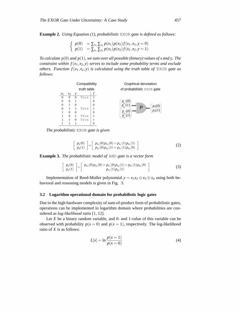
Example 2. Using Equation (1), probabilisticEXOR gate is defined as follows:{
p(0) = ∑x1 ∑x2p(x1)p(x2) f (x1,x2,y = 0)
p(1) = ∑x1 ∑x2p(x1)p(x2) f (x1,x2,y = 1)
To calculate p(0) and p(1), we sum over all possible (binary) values of x and y. Theconstraint within f(x1,x2,y) serves to include some probability terms and excludeothers. Function f(x1,x2,y) is calculated using the truth table ofEXOR gate asfollows:
Compatibility Graphical denotation
truth table of probabilistic EXOR gatex1 x2 y f0 0 0 TRUE 10 0 1 00 1 0 00 1 1 TRUE 11 0 0 01 0 1 TRUE 11 1 0 TRUE 11 1 1 0
py(0) py(1)
x1 p (0) x1 p (1)
x2 p (0) x2 p (1)
P
The probabilisticEXOR gate is given
[py(0)py(1)
]
=
[px1(0)px2(0)+ px1(1)px2(1)px1(0)px2(1)+ px1(1)px2(0)
]
(2)
Example 3. The probabilistic model ofAND gate is a vector form[
py(0)py(1)
]
=
[px1(0)px2(0)+ px1(0)px2(1)+ px1(1)px2(0)
px1(1)px2(1)
]
(3)
Implementation of Reed-Muller polynomialy = x1x2⊕ x3⊕ x4 using both be-havioral and reasoning models is given in Fig. 3.
3.2 Logarithm operational domain for probabilistic logic gates
Due to the high hardware complexity of sum-of-product form of probabilistic gates,operations can be implemented in logarithm domain where probabilities are con-sidered aslog-likelihood ratio[1, 12].
Let X be a binary random variable, and 0- and 1-value of this variable can beobserved with probabilityp(x = 0) andp(x = 1), respectively. The log-likelihoodratio ofX is as follows:
L[x] = lnp(x = 1)
p(x = 0)(4)

458 S. N. Yanushkevich et al.:
Table 1. The sum-of-product and log-likelihood forms of AND and EXOR probabilistic logic gatemodels.
S u m - o f - p r o d u c t m o d e l
Probabilistic AND Probabilistic EXOR
py(0) py(1)
x1 p (0) x1 p (1)
x2 p (0) x2 p (1)
P py(0)
py(1)
x1 p (0) x1 p (1)
x2 p (0) x2 p (1)
P
x1 x2 y f0 0 0 10 0 1 00 1 0 10 1 1 01 0 0 11 0 1 01 1 0 01 1 1 1
x1 x2 y f0 0 0 10 0 1 00 1 0 00 1 1 11 0 0 01 0 1 11 1 0 11 1 1 0
Probabilistic model: see equation (2) Probabilistic model: see equation (3
L o g - l i k e l i h o o d m o d e l
Probabilistic AND Probabilistic EXOR
L[x1] P L[x2]
L[y]
L[x1] L[x2]
L[y] P
L[y] = L[x1x2]
= MAX (|L[x1]|, |L[x2]|)
L[y] = L[x1⊕x2]
= SGN(L[x1])SGN(L[x2])
×MIN (|L[x1]|, |L[x2]|)
The probabilityp(x = 0) can be recovered from Equation 4:
p(x = 0) =eL[x]
1+eL[x]
Operations in the logarithm domain are specified by properties of log-likelihoodratio model of probabilistic logic gate (Equation 4), in particular, multiplication ofreal numbers is translating into additions.
The AND and EXOR probabilistic logic gates based on log-likelihood ratiomodel (Equation 4) are used to design belief propagation networks.
Example 4. The design goal of decoder of turbo error correcting codes is to prop-agate the belief efficiently. Specifically, the sign and magnitude of|L[x]| (belief) areestimated, and then improving these estimates using the local redundancy of the

The EXOR Gate Under Uncertainty: A Case Study 459
Design example: Reed-Muller Design example: Reed-Mullernetwork design using network design using
behavioral model reasoning modelGiven:
(a) a switching function y= x1x2⊕x3⊕x4,(b) the binary input signals x1,x2,x3, and
x4 are independent,(c) the probabilities of 1’s in the input
streams,p(x1) = p(x2) = p(x3) = p(x4) = 0.8
Design a probabilistic logic network us-ing behavioral model, and calculate p(y).
Given:
(a) a switching function y = x1x2⊕x3⊕x4,(b) the input binary signals x1,x2,x3, and x4
are independent,(c) the probabilities of the input signals,
px1(0) = · · ·= px4(0) = 0.2 and px1(1) =· · ·= px4(1) = 0.8.
Design a probabilistic logic network to imple-ment function y using reasoning model, andcalculate p(y).
Solution:Step 1: Design Type I probabilistic logicnetwork:
x3 x4
y2
x1 x2
y1
y3
Random binary inputs
p(x1)
p(x2)
p(x3)
p(x4)
p(y1) p(y2)
p(y3)
Random binary output
Solution: Step 1: Design Type II probabilisticlogic network:
Input probabilities
Output probability
P
P
y3 p (0) y3
p (1)
y2 p (0) p (1) y2
y1 p (0) p (1) y1
x1 p (0) x1 p (1) x2
p (0)
x2 p (1) x3
p (0) x3 p (1) x4
p (0) x4
p (1)
P
Step 2: Using behavioral models
p(y1) =p(x1)p(x2) = 0.8×0.8 = 0.64
p(y2) =p(x3)+ p(x4)−2p(x3)p(x4)
=0.8+0.8−2×0.8×0.8 = 0.32
p(y3) =p(y1)+ p(y2)−2p(y1)p(y2)
=0.64+0.32−2×0.64×0.32
= 0.5504
Step 2: Using Equations 2 and 3[
py1(0)py1(1)
]
=
[ 0.2·0.2+0.2·0.8+0.8·0.2 = 0.36
0.8×0.8 = 0.64
]
[py2(0)py2(1)
]
=
[ 0.2×0.2+0.8×0.8 = 0.68
0.2×0.8+0.8×0.2 = 0.32
]
[py3(0)py3(1)
]
=
[ 0.36·0.68+0.64·0.32= 0.4496
0.36·0.32+0.64·0.68= 0.5504
]
Fig. 3. Reed-Muller probabilistic network design using behavioral (left) and reasoning (right) models.
code. The result of this belief propagation can be written as iterative process:
Lt+1[x] = Lt [x]+ p(x), t = 1,2, . . . ,m,
where p(x) is the probabilistic quantity, orextrinsicinformation about x.
In Table 1, the log-likelihood ratio model is given for two-input AND andEXOR gates assuming that binary variablesx1 andx2 are statistically independent.
460 S. N. Yanushkevich et al.:
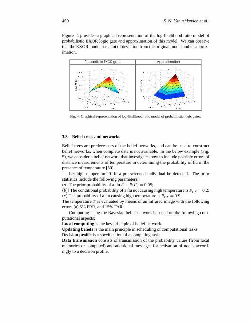
Figure 4 provides a graphical representation of the log-likelihood ratio model ofprobabilistic EXOR logic gate and approximation of this model. We can observethat the EXOR model has a lot of deviation from the original model and its approx-imation.
Probabilistic EXOR gate Approximation
Fig. 4. Graphical representation of log-likelihood ratio model of probabilistic logic gates.
3.3 Belief trees and networks
Belief trees are predecessors of the belief networks, and can be usedto constructbelief networks, when complete data is not available. In the below example (Fig.5), we consider a belief network that investigates how to include possible errors ofdistance measurements of temperature in determining the probability of flu in thepresence of temperature [30].
Let high temperatureT in a pre-screened individual be detected. The priorstatistics include the following parameters:(a) The prior probability of a fluF is P(F) = 0.05;(b)] The conditional probability of a flu not causing high temperature isPT|F = 0.2;(c) The probability of a flu causing high temperature isPT|F = 0.9.The temperatureT is evaluated by means of an infrared image with the followingerrors (a) 5% FRR, and 15% FAR.
Computing using the Bayesian belief network is based on the following com-putational aspects:Local computing is the key principle of belief network.Updating beliefs is the main principle in scheduling of computational tasks.Decision profile is a specification of a computing task.Data transmissionconsists of transmission of the probability values (from localmemories or computed) and additional messages for activation of nodes accord-ingly to a decision profile.

The EXOR Gate Under Uncertainty: A Case Study 461
Reasoning with Bayesian networks is done by updating beliefs, that is, comput-ing the posterior probability distributions, given new information, calledevidence.The basic idea is that new evidence has to be propagated to the other parts of thenetwork.
Fundamental expansion for belief networks
A Bayesian belief networks is a graphical representation of a chain rule;that is, a factored representation of joint probability distribution in the form
P(x1,x2, . . . ,xn) =
=
Factored form︷ ︸︸ ︷
P(x1)×P(x2|x1)× . . . ,P(xn|x1, . . . ,xn−1)
= ∏i
P(xi |x1,x2, . . . ,xi−1)
︸ ︷︷ ︸
Chain rule
⇔m
∏i=1
P(xi |Par(Xi)
︸ ︷︷ ︸
Graphical representation
where Par(Xi) denotes a set of parent nodes of the random variable xi . Thenodes outside Par(Xi) are conditionally independent of xi .
Prior
PT |F =0.8 PT |F =0.2 PT |F =0.1 PT |F =0.9
PF =0.05 PF =0.95
000 001 010 011
PM |T PM |T =0.15 PM |T
PM |T =0.95 M M
PM |T PM |T =0.15
PM |T PM |T =0.95
M M
T T
100 101 110 111
Posterior (belief) probabilities
High temperature
Measure
Layer 1
Layer 2
Layer 3
F
Infrared camera
Image processing
Fig. 5. Probabilistic network as belief tree.
4 Stochastic model
Stochastic model is a typical computational paradigm, which utilizes statistical av-eraging in data representation and manipulation, such as addition, subtraction, mul-tiplication, and division. Because of data averaging, these operations are highlyimmune to noise.

462 S. N. Yanushkevich et al.:
A binary stochastic pulse stream is defined as a sequence of binary digits,orbits. The information in a pulse stream is contained in the primary statistics ofthe bit stream, or the probability of any given bit in the stream being a logic 1.Hence, the output of a gate is generally in the form of a nonstationary Bernoullisequence (random process of repeated trials with two possible outcomes;this pro-cess is characterized by the binomial distribution) [8, 4, 10]. Such a sequence canbe considered in probabilistic terms as adeterministic signal with superimposednoise. Suppose that the statistical characteristics of these streams are known, andcan be measured. These streams carry a signal by statistical characteristics (a singleevent carries very little information, which is not enough for decision making).
Example 5. Let the binary variables x1 and x2 correspond to the stochastic pulsesignals with the means E(x1) and E(x2). Suppose that these pulse streams areindependent. It is possible to find some logic operations that correspondto the sumE(x1)+E(x2) and the product E(x1)×E(x2).
If the input stochastic streams are independent (technically, this means thatindependent generators of random pulses are used with some additionaltools fordecorrelation of signals), and are represented byE(x1) andE(x2), the output ofgate is described by the equationE( f ) = E(x1)×E(x2). The values are normalizedinto the range[0,1].
Pulse stream
E(x1)
Pulse stream E(x2)
E( f )
Pulse stream
Fig. 6. Stochastic pulse stream model of computing.
The stochastic computer introduces its own errors in the form ofrandom vari-ance. If we observe a sequence ofN logic levels andk of them are 1, then theestimated probability is ˆp = k/N. The sampling distribution of the value ofk is bi-nomial, and, hence, the standard deviation of the estimated probability ˆp from thetrue probabilityp is σ(p) = [p(1− p)/N]1/2. Therefore, the accuracy in estimationof the generated probability increases as the square root of the length, or time, ofcomputation.
Let p1 = E(x1) andp2 = E(x2), then:(a) The AND gatef = x1x2 is modeled byE( f ) = p1p2, if input pulse streams are

The EXOR Gate Under Uncertainty: A Case Study 463
independent, and byE( f ) = p1p2 +Kx1,x2 otherwise;(d) The EXOR gatef = x1⊕x2 is modeled byE( f ) = p1+ p2−2p1p2, if the inputpulse streams are independent, and byE( f ) = p1+ p2−2p1p2−2Kx1,x2 otherwise.(e) The XNOR gatef = x1⊕x2 is modeled byE( f ) = 1− p1− p2 +2p1p2 if theinput pulse streams are independent. Here,Kx1,x2 is correlation function.
The precision of computing depends on the size of the stochastic sequence.This effect can be evaluated by standard statistical techniques. LetX be a binomialrandom variable; then the limiting form of the distribution is the normal distribu-tion. Given a precision of computationε, the result of computing must satisfy theequation|k/n− p(x)| ≤ ε. The confidence interval is
−ε√
np(x)q(x)
≤k−np(x)
√
np(x)q(x)≤ ε
√n
p(x)q(x)
The size of Bernoulli stream isn = (zα2
pq/ε)2. In practice, the sizen variesfrom hundreds to thousands, depending on the required precision of computations.
The most reasonable stochastic pulse encoding models areone-bit addersandone-bit multipliers. A simple rule for describing the model is used, such that itreplaces the Boolean variablexi in an arithmetic equation by the meanE[xi ] of thestochastic sequence [8, 14, 17, 28].
5 Decision diagram model
A decision diagram is a graphical data structure in the form of a rooted directedacyclic graph, consisting of the root node, a set of non-terminal nodesand a set ofterminal (constant) nodes connected via directed edges (links). The topology of adecision diagram is characterized by the parameters such as size, numberof non-terminal nodes, number of links, and shape. The computing paradigm underlyingdecision diagrams is based on the hierarchical decomposition of a logic function(each level corresponds to a single variable). Each path from the rootnode to aterminal node represents a term in the algebraic description of the function.
An arbitrary logic function can be implemented using decision diagrams, inwhich nodes are multiplexers, or switches. The library of multiplexer-basedimple-mentations is given in Fig. 7. This model is a good candidate for implementationusing molecular switches [11].
5.1 Experiments
The goal of this experiment is to model some unreliable gates with the introductionof noise of various scales and observe the deviation of the output value from the

464 S. N. Yanushkevich et al.:
AND gate EXOR gate
x1
x2
f ⇒
f
0 1 s(x1)
f
0 I2(x2)
x1
x2
f
⇒
f
0 1 s(x1)
f
I1(x2)
f = 0×s∨ I2×s= x1x2 f = I1×s∨ I1×s= x1⊕x2
x1
1
0
x2
f
0 1
0 1 x1
1
f
0 1
x2 0 1 0 1
x2
0 0
Fig. 7. Switch based AND/EXOR library.
actual one. We consider line noise (any line connecting nodes of the diagram)and node noise (any node within diagram) models. The noise (r) is either additive(modeled via OR gate) or multiplicative (modeled via AND gate). The latter noisemodel is shown in the form of AND gates, added to the lines and to the selectedinput of multiplexers in Fig. 8a.
1
0 1
f
0 1 x1
r
x2
0
r r r
1
x1
x2
r
0 1
f
0 1
0
(a) (b)
Fig. 8. Complete (a) and one-line (b) noise-injected AND gate model.
Fig. 9 shows the results of simulation of the output probability (axis Z) forAND (a) and EXOR (b) while varying multiplicative noise on one line only. Theline between terminal node 1 and the lower MUX was chosen for for AND gatemodel, and the line between terminal node 1 and the lower right MUX for EXORgate model, whilep(x1 = 1) = 1 (inputx1 is constant 1), and the probabilitiesp(x2)andp(r) vary between 0 and 1 on axes X and Y.

The EXOR Gate Under Uncertainty: A Case Study 465
(a) (b)
Fig. 9. Graphical representation of the probabilistic AND (a) and EXOR (b) model based on noise-injected decision diagram.
6 Neuromorphic model
Neuromorphic networks are hardware implementation of artificial neural networks,they resemble cooperative phenomena, and can process probabilistic, noisy, or in-consistent information [13].
The Hopfield computing paradigm is based on the concept ofenergy minimiza-tion in a stochastic system [9]. Control over the type of logic function is exercisedby the thresholdθ and the weightswi ∈ {1,−1} in the arithmetic sum representingthe output value,f = w1×x1 +w2×x2−θ .
Hopfield networks are capable of reliable computing, despite imperfect neuroncells and degradation of their performance. This is because the degraded neuroncells store information (in weights, thresholds, and topology) in adistributed(orredundant) manner. A single “portion” of information is not encoded in a singleneuron cell but is rather spread over many. Boolean function is computedvia aprocess called “simulated annealing”. A value of a Boolean function, given anassignment of its Boolean variables, is computed through relaxation of the neuroncells in the network, while the initial “temperature” of the network is given.
A set of fundamental two-input logic functions can be implemented as a three-node Hopfield network. The logic functions AND and EXOR are shown in Table 2.The logic function AND can be implemented using a three-node Hopfield network,and EXOR requires a four-node Hopfield network. The Boolean function of alogic gate is encoded in the energy function, using connection weights and neuronthreshold. The energy function of the network is defined as follows:
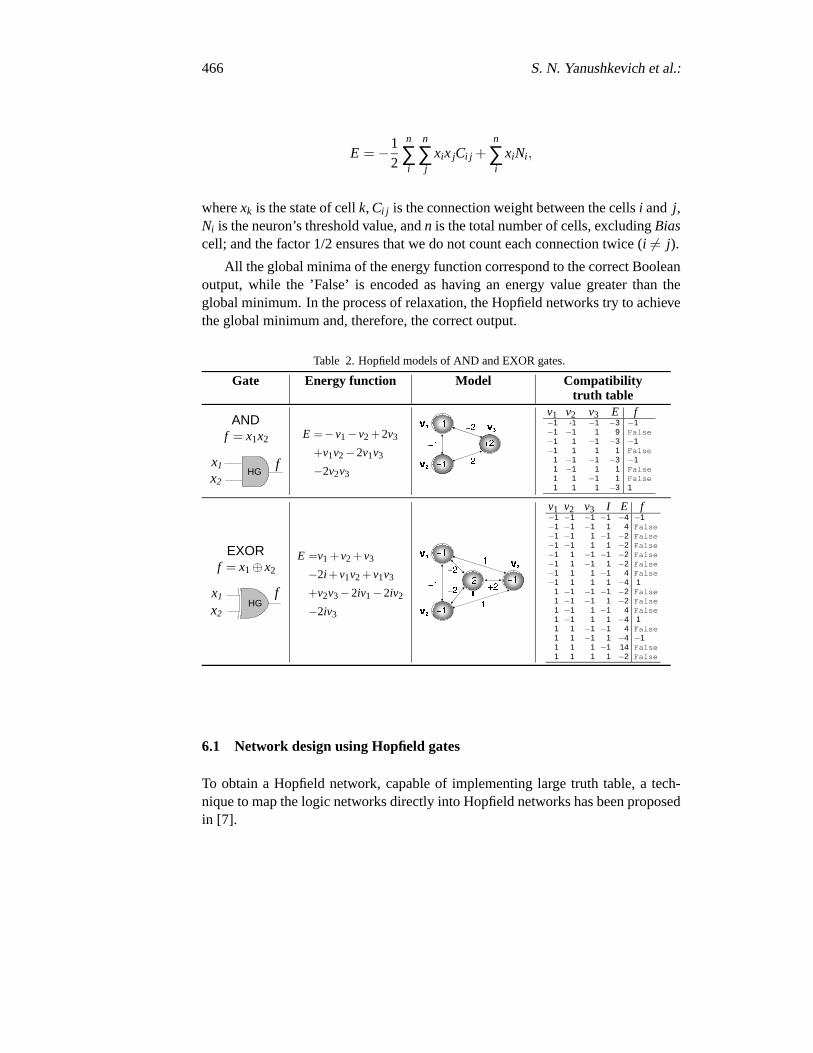
466 S. N. Yanushkevich et al.:
E =−12
n
∑i
n
∑j
xix jCi j +n
∑i
xiNi ,
wherexk is the state of cellk, Ci j is the connection weight between the cellsi and j,Ni is the neuron’s threshold value, andn is the total number of cells, excludingBiascell; and the factor 1/2 ensures that we do not count each connection twice (i 6= j).
All the global minima of the energy function correspond to the correct Booleanoutput, while the ’False’ is encoded as having an energy value greater than theglobal minimum. In the process of relaxation, the Hopfield networks try to achievethe global minimum and, therefore, the correct output.
Table 2. Hopfield models of AND and EXOR gates.
Gate Energy function Model Compatibilitytruth table
ANDf = x1x2
x1
x2
f HG
E =−v1−v2 +2v3
+v1v2−2v1v3
−2v2v3
v1 v2 v3 E f−1 -1 −1 −3 −1−1 −1 1 9 False−1 1 −1 −3 −1−1 1 1 1 False
1 −1 −1 −3 −11 −1 1 1 False1 1 −1 1 False1 1 1 −3 1
EXORf = x1⊕x2
x1
x2
f HG
E =v1 +v2 +v3
−2i +v1v2 +v1v3
+v2v3−2iv1−2iv2
−2iv3
v1 v2 v3 I E f−1 −1 −1 −1 −4 −1−1 −1 −1 1 4 False−1 −1 1 −1 −2 False−1 −1 1 1 −2 False−1 1 −1 −1 −2 False−1 1 −1 1 −2 False−1 1 1 −1 4 False−1 1 1 1 −4 1
1 −1 −1 −1 −2 False1 −1 −1 1 −2 False1 −1 1 −1 4 False1 −1 1 1 −4 11 1 −1 −1 4 False1 1 −1 1 −4 −11 1 1 −1 14 False1 1 1 1 −2 False
6.1 Network design using Hopfield gates
To obtain a Hopfield network, capable of implementing large truth table, a tech-nique to map the logic networks directly into Hopfield networks has been proposedin [7].

The EXOR Gate Under Uncertainty: A Case Study 467
Rule I: Hopfield gate merging
Connecting an output of one Hopfield gate to the input of another (cas-cading the gates) is performed by merging the corresponding “output”cell of the first gate with the “input” cell of the second one. The thresholdvalue of the new cell is the cumulative threshold of the merged cells.
Rule II: Hopfield gate merging
Connecting an output of one Hopfield gate to the input of another (cas-cading the gates), while the second input of the other gate is also theinput of the first one, is performed by merging the corresponding “out-put” cell of the first gate with the “input” cell of the second one, as wellas the both ”input” cells. The threshold value of the two new cells is thecumulative threshold of the merged cells.
Example 6. Rule I: While connecting AND and EXOR gate, both cells G1 aremerged in a new cell, which threshold value is 2+1=3, obtained by adding thethreshold values of the merged cells (Fig. 10, upper plane).
A p p l i c a t i o n o f m e r g i n g R u l e I
−−−−1
−−−−1
2
2
2
−−−−1
X1
X2
G1G1G1G1
ANDANDANDAND
+
1
1
1
−−−−1
−−−−1
−−−−1
G1G1G1G1
X3
G2
XXXXOROROROR
−−−−2 2
2
2
=
=
Fig. 10. Taxonomy of neuromorphic AND/EXOR network design: application of merging rules inimplementation of functionf = x1x2⊕x3.
Example 7. Rule II: Input x2 is common for both AND and EXOR gates, so theircascading involves merging gates X2 and G1, and their threshold are cumulativevalues, -1+1=0 and 2+1=3, respectively (Fig. 10, lower plane).
6.2 Noise Model for the Hopfield networks
In this paper, to investigate fault tolerance of the Hopfield networks, a discretenoise is added in the form of noise probability. Noise probability is defined here as

468 S. N. Yanushkevich et al.:
A p p l i c a t i o n o f m e r g i n g R u l e II
−−−−1
−−−−1
2
2
2
−−−−1
X1
XXXX2222
G1G1G1G1
ANDANDANDAND
+
1
1
1
−−−−1
−−−−1
−−−−1
G1G1G1G1
X3X3X3X3
G2
XXXXOROROROR
−−−−2 2
2
2
=
=
Fig. 10. (Continue) Taxonomy of neuromorphic AND/EXOR network design: application of mergingrules in implementation of functionf = x1x2⊕x3.
the probability that a neuron cell is affected by noise resulting in a bit flip, called“a state flip” in terms of Hopfield networks. In other words, change of the stateis modelled by the uniformly distributed discrete random signal. For example,noise level 0.1 (10%) means that the probability of changing the current state of theneuron cell is 0.1.
There are two updating rules that applies to the Hopfield network: (a) the Hop-field deterministic rule, and (b) stochastic Boltzmann rule, or simulated annealing.For example, the Boltzmann updating rule is based on assumption of an uncertaintyof state of a particular cell during the updating process. Instead of settingthe stateof cell k deterministically, the process uses the probabilityp(k) that cellk takesstate 1. It implies the following steps: (a) Select temperatureT; (b) Randomly se-lect a cellk, (c) Calculate∆E(k) = ∑n
i xicik−Nk. If ∆E(k) > 0, then calculate theprobability that cellk takes state 1:p(k) = 1
1+e−∆E(k)/T . Else set the state of cellkto -1; (d) Repeat steps (b) through (d) until the state of cell does not change for acertain interval (this is also called stable state condition), for example, 20 iterations.
6.3 Experimental Results
In this study, we have compared the robustness of the Hopfield models for EXORgate using the 4-node Hopfield EXOR gate (f = x⊕ y), and the alternative imple-mentations of EXOR: one in the form off = xy∨ xy using the network of one2-node Hopfield NOT gate, two 3-node AND gates and one 3-node OR gate, andanother in the formf = x ·xy∨xy·y.
Example 8. Given the node noise probability ranging between 0 and0.5, the num-ber of iteration to reach the stable state vary for the EXOR Hopfield gate itself

The EXOR Gate Under Uncertainty: A Case Study 469
(Figure 11, A), and for the implementation of EXOR on a network of NOT, ANDand OR gates (B), as well as a network of NAND, AND and OR gates. The lattertwo seem to need less iteration, while the noise level increases beyond 0.2, andis significantly different for noise level 0.5. The EXOR gate itself (which requiresfour neurons) required much more iterations to achieve the correct output, whilethe networks of NOT, AND, OR or NAND gates, each consisting of two (NOTonly)or three neurons), connected in the network with total 10 (B) and 15 neurons (C),respectively, are mush faster to reach the stable state.
Fig. 11. Behavioral characteristics of neuromorphic model: X and Y axes correspond the level ofnoise and number of required iterations to reach stable state condition, respectively; the curves A, Band C correspond to EXOR gate, and the network of NOT, AND, OR, and NAND, AND and OR,implementing the same EXOR function, respectively.
On the other hand, even if the EXOR Hopfield gate is much slower in achievingthe stable condition, it is more robust than the network of AND, OR or NANDgates, implementing the same function EXOR.
Example 9. Given the node noise probability ranging between 0 and0.5, the prob-ability of achieving the correct output is better for the EXOR Hopfield gate itself(Figure 12, A), and for the implementation of EXOR on a network of NAND, ANDand OR gates (C), while the probability of achieveing the correct output forthenetwork of NOT, AND and OR gates (B) is only around 0.6.
Another experimental study of performance on the Hopfield networks, imple-menting simple AND-EXOR expressions, have been performed using the circuitsx1x2⊕ x3x4. This experiment compares the probability of achieving the correctoutput of the benchmark, for both logic network and Hopfield network with noise.
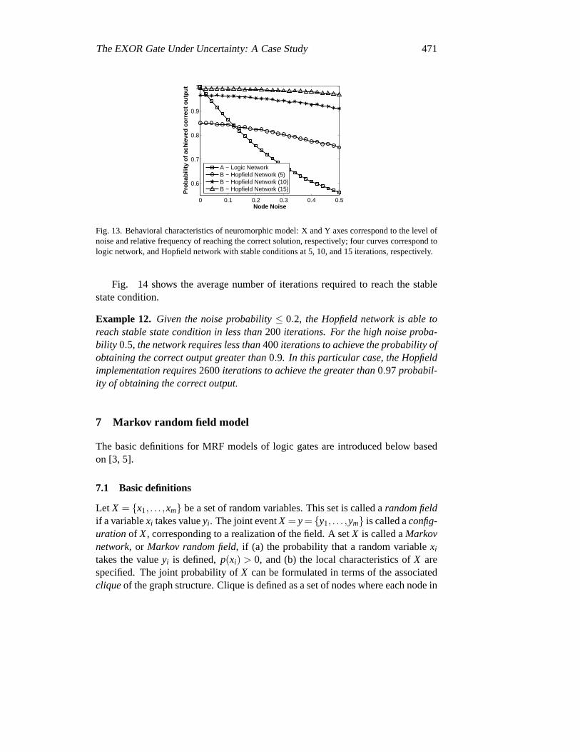
Fig. 13 shows the probability of correct output with respect to the noise prob-ability ranging from 0 to 0.5. The stable state condition for the Hopfield network
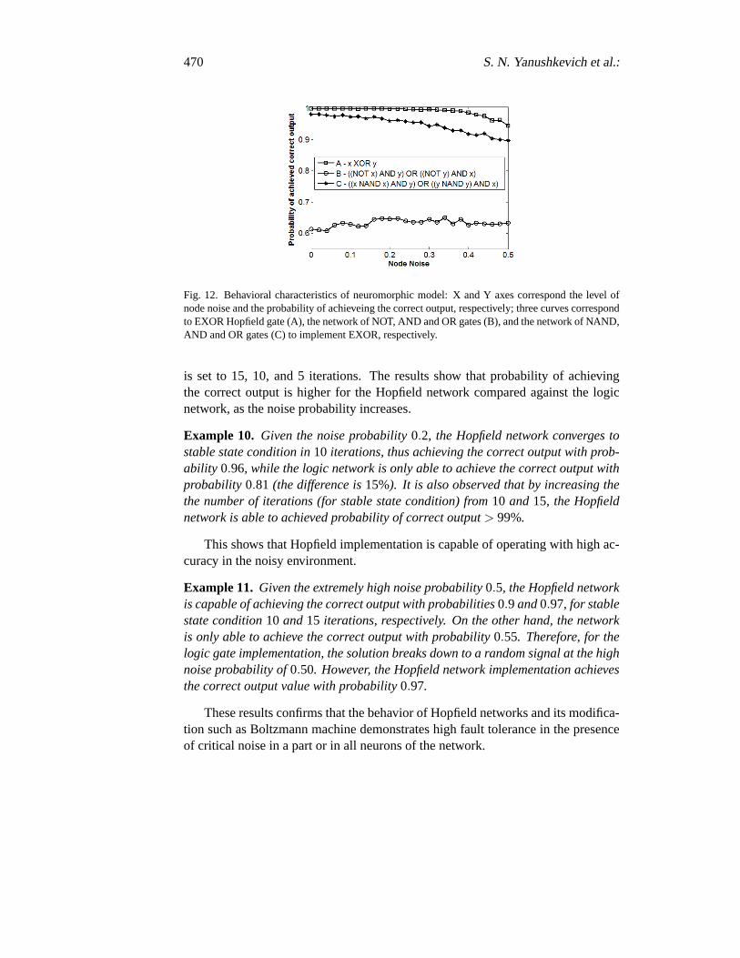
470 S. N. Yanushkevich et al.:
Fig. 12. Behavioral characteristics of neuromorphic model: X and Y axes correspond the level ofnode noise and the probability of achieveing the correct output, respectively; three curves correspondto EXOR Hopfield gate (A), the network of NOT, AND and OR gates (B), andthe network of NAND,AND and OR gates (C) to implement EXOR, respectively.
is set to 15, 10, and 5 iterations. The results show that probability of achievingthe correct output is higher for the Hopfield network compared against the logicnetwork, as the noise probability increases.
Example 10. Given the noise probability0.2, the Hopfield network converges tostable state condition in10 iterations, thus achieving the correct output with prob-ability 0.96, while the logic network is only able to achieve the correct output withprobability 0.81 (the difference is15%). It is also observed that by increasing thethe number of iterations (for stable state condition) from10 and15, the Hopfieldnetwork is able to achieved probability of correct output> 99%.
This shows that Hopfield implementation is capable of operating with high ac-curacy in the noisy environment.
Example 11. Given the extremely high noise probability0.5, the Hopfield networkis capable of achieving the correct output with probabilities0.9 and0.97, for stablestate condition10 and15 iterations, respectively. On the other hand, the networkis only able to achieve the correct output with probability0.55. Therefore, for thelogic gate implementation, the solution breaks down to a random signal at the highnoise probability of0.50. However, the Hopfield network implementation achievesthe correct output value with probability0.97.
These results confirms that the behavior of Hopfield networks and its modifica-tion such as Boltzmann machine demonstrates high fault tolerance in the presenceof critical noise in a part or in all neurons of the network.
The EXOR Gate Under Uncertainty: A Case Study 471
0 0.1 0.2 0.3 0.4 0.5
0.6
0.7
0.8
0.9
1
Node Noise
Pro
babi
lity
of a
chie
ved
corr
ect o
utpu
t
A − Logic NetworkB − Hopfield Network (5)B − Hopfield Network (10)B − Hopfield Network (15)
Fig. 13. Behavioral characteristics of neuromorphic model: X and Y axes correspond to the level ofnoise and relative frequency of reaching the correct solution, respectively; four curves correspond tologic network, and Hopfield network with stable conditions at 5, 10, and 15 iterations, respectively.
Fig. 14 shows the average number of iterations required to reach the stablestate condition.
Example 12. Given the noise probability≤ 0.2, the Hopfield network is able toreach stable state condition in less than200 iterations. For the high noise proba-bility 0.5, the network requires less than400iterations to achieve the probability ofobtaining the correct output greater than0.9. In this particular case, the Hopfieldimplementation requires2600iterations to achieve the greater than0.97probabil-ity of obtaining the correct output.
7 Markov random field model
The basic definitions for MRF models of logic gates are introduced below basedon [3, 5].
7.1 Basic definitions
Let X = {x1, . . . ,xm} be a set of random variables. This set is called arandom fieldif a variablexi takes valueyi . The joint eventX = y= {y1, . . . ,ym} is called aconfig-urationof X, corresponding to a realization of the field. A setX is called aMarkovnetwork, or Markov random field, if (a) the probability that a random variablexi
takes the valueyi is defined,p(xi) > 0, and (b) the local characteristics ofX arespecified. The joint probability ofX can be formulated in terms of the associatedcliqueof the graph structure. Clique is defined as a set of nodes where each node in

472 S. N. Yanushkevich et al.:
0 0.1 0.2 0.3 0.4 0.50
500
1000
1500
2000
2500
3000
Connection and Functional Noise
Ave
rage
num
ber
of It
erat
ions
A − 15 IterationsB − 10 IterationsC − 5 Iterations
Fig. 14. Behavioral characteristics of neuromorphic model: X and Y axes correspond the level ofnoise and number of required iterations to reach stable state condition, respectively; three curvescorrespond to 5, 10, and 15 iterations, respectively.
the set connects to other nodes in the graph. The conditional probability ofa nodeonly depends on its neighborhood. This model considers the effects of noise andother uncertainty factors on a node by considering the conditional probabilities ofenergy values with respect to its clique.
7.2 Concept of energy of a logic function
In MRF model, computing the simplest logic operations in the presence of noise,such as NOT, AND, NAND, OR, is performed using notation of energy. The “en-ergy” of a logic function is accumulated by “potentials” of cliques. This terminol-ogy comes from statistical physics.
Given a cliquec ∈ C, a clique potential, Vc(x), is a non-negative real-valuedfunction of this particular clique. It follows from this definition that a logic functionmust be represented in a particular form, such that arithmetic operations areusedinstead of logic ones.
Example 13. A complete graph with three nodes v1,v2 and v3 is a clique, becauseall distinct pairs of nodes, v1,v2, v1,v3, and v2,v3 are neighbors.
A sum of clique potentials,Vc(x), over all possible cliquesC is called theenergyfunction, and is denoted as
E(x) = ∑c∈C
Vc(x) (5)
The energy function is a quantitative measure of the global quality of the solu-tion; the correct solution corresponds to the maximum of energy function. Note

The EXOR Gate Under Uncertainty: A Case Study 473
that in this paper, we consider logic primitivesf (x1,x2), which are represented bycomplete graph (a single clique model); that is, energyE(x) is equal to a cliquepotential:E(x) = Vc=1(x) = V(x).
Gibbs joint probability distributionor Gibbs random field, is defined in theform
p(X = x) =1Z
exp
(E(x)kT
)
(6)
whereZ is a scaling factor (to normalize the total probability to 1) andkT is thetemperature factor (in physics view,T is “temperature”, andk is Boltzmann con-stant).
Given a joint probability distributionp(x1, . . . ,xr), themarginal distributionis defined as follows:
p(x1, . . . ,xs) = ∑xs+1,...,xr
p(x1, . . . ,xr), s≤ r
Marginal distribution can be viewed as a projection of the joint distribution on asmaller set of variables.
Hence, Gibbs random fields is defined by a joint probability. On the contrary,the MRF is based on a conditional probability. The equivalence between theMRFand the Gibbs random field can be established by the following theorem.
Hammersley-Clifford theorem states that a set of random variablesX ={x1, . . . ,xs} is a MRF, if and only ifX is Gibbs distributed. That is, the globalprobabilistic characteristics can be computed using local interactions via factoriza-tion. Specifically, the joint probability of an MRF can be constructed from thelocalconditional probabilities.
Logic function is incorporated into a Markov network using anarithmeticforms[24, 23].
7.3 Algorithm for synthesis of MRF models of logic gates
Given the compatibility truth vectorU of a Boolean functionf of n variables, thevector of coefficientsA = (a1,a2, . . . ,an) is calculated using the arithmetic trans-form [23]:
A = A2n ·U (7)
where matrixA2n is formed as follows
A2n =n⊗
j=1
A2 j , A21 =[
1 0−1 1
]

474 S. N. Yanushkevich et al.:
Arithmetic formof r-input,x1,x2, . . . ,xr , logic gatef , given by spectral coeffi-cients,a1,a2, . . . ,an is defined by the polynomial:
f =2r−1
∑i=0
ai · (xi11 · · · xir
r ), (8)
where i j is the j-th bit 1,2, . . . , r, in the binary representation of the indexi =
i1i2 . . . ir ; xi jj = 1 if i j = 0, andx
i jj = x j if i j = 1.
Example 14. Arithmetic representation of a 3-input logic gate (n= 3) is definedby Equation (8) as follows: f= a0 + a1x3 + a2x2 + a3(x2x3)+ a4x1 + a5(x1x3)+a6(x1x2)+a7(x1x2x3).
Consider a 2-input logic gate of a functionL. The algorithm for designing theMRF model of this gate is as follows.
The MRF model design for a 2-input logic gate
Input data: (a) Graph model {v1,v2,v3} (complete graph) and(b) function L.Step 1: Form the compatibility truth table.Step 2: Calculate the energy function, E(v), usingFourier-like transform, in particular, arithmetictransform (7).Step 3: Specify Gibbs distribution (6) by substitutingthe energy function, E(v), into it.Step 4: Calculate the marginal probability distributionof the output node.Output: An MRF model of L gate.
Designing the MRF model for the AND gate is illustrated by the followingexample (Fig. 15).
Table 3 provides design results for two-input OR and EXOR gate. It is shownin Table 3, that the valid input/output states have higher clique energies than invalidstates to maximize the probability of a valid energy state at the nodes:E(v) of validstates is 1, and for any invalid state, this value is 0. The logic margin in this caseis the difference between the probabilities of occurrence of a logic low anda logichigh, which, if high, leads to a higher probability of correct computation.
Further applying the belief propagation algorithm, the energy distributions andentropy at different nodes of the network can be calculated [24].
These MRF models show that maximization of logic state probability can beviewed as a process of energy maximization. Note that energy minimization pro-cess can be achieved by sign manipulation in compatibility truth table and Gibbs

The EXOR Gate Under Uncertainty: A Case Study 475
Design example:MRF model for logic 2-input AND gate
Given:
(a) Complete noncausal graph, {v1,v2,v3}(b) Logic function of gate L
Design an MRF model of L gate.Solution:Step 1: Form the compatibility truth table:
v1 v2 v3 U Comment0 0 0 10 0 1 0 Undesirable0 1 0 10 1 1 0 Undesirable1 0 0 11 0 1 0 Undesirable1 1 0 0 Undesirable1 1 1 1
Step 2: Calculate the energy function, U(v):(a) Calculate a clique potential using arithmetic transform (7):
A = A23 ·U =
1 0 0 0 0 0 0 0−1 1 0 0 0 0 0 0−1 0 1 0 0 0 0 0
1 −1 −1 1 0 0 0 0−1 0 0 0 1 0 0 0
1 −1 0 0 −1 1 0 01 0 −1 0 −1 0 1 0−1 1 1 −1 1 −1 −1 1
10101001
=
1−1
0000−1
2
(b) Convert the vector of coefficients A into algebraic form using equation (8):E(v) = 1−v3−v1v2 +2v1v2v3Step 3: Specify Gibbs distribution:
p(v1,v2,v3) =1Z
exp
(1−v3−v1v2 +2v1v2v3
kT
)
Step 4: (a) Calculate marginal distribution by summing over all possible states of v1:
p(v2,v3) =1Z1
∑v1∈0,1
exp
(1−v3−v1v2 +2v1v2v3
kT
)
=1Z1
[
exp
(1−v3
kT
)
+exp
(1−v3−v2 +2v2v3
kT
)]
Fig. 15. MRF-based model for AND gate.

476 S. N. Yanushkevich et al.:
(b) Calculate marginal distribution of v3 by summing over all possible states of v2:
p(v3) =1Z2
∑v2∈0,1
[
exp
(1−v3
kT
)
+exp
(1−v3−v2 +2v2v3
kT
)]
=1Z2
[
3exp
(1−v3
kT
)
+exp
(v3
kT
)]
0 0.2 0.4 0.6 0.8 10
0.1
0.2
0.3
0.4
0.5
Output, V3
Pro
babi
lity,
p(V
3)
kT=0.1kT=0.25kT=0.5kT=1
Fig. 15. (Continue) MRF-based model for AND gate.
distribution. Therefore, a bistable storage element with feedback is an appropriatehardware architecture for binary logic [19, 31].
8 Conclusion and discussion
An extended vision of probabilistic network design, including probabilistic AND-EXOR networks, is introduced. This interdisciplinary view includes the field ofcoding for error correction based on statistical techniques, and belief networks fordecision making. In these fields, data processing is based on probabilistic andstatistic techniques, using both discrete and analog technology for implementationof computing networks over the libraries of probabilistic logic gates.
There exists a diversity in terminology related to probabilistic computing. Forexample, the term “probabilistic EXOR gate” addresses the following meanings:
(a) traditional EXOR gate assuming random input and output signals (we pro-posed to distinguish this meaning as “behavioral model”), and
(b) computing device which operates with probabilities (real numbers) with re-spect to EXOR switching function (in our systematization, it is a “ beliefmodel”).

The
EX
OR
Gate
Under
Uncertainty:
AC
aseS
tudy477
Table 3. Components of the MRF model of binary gates.
Gate Graph model Compatibility Clique potential Probabilistictruth table (arithmetic form of gate) behavior
x1
x2
f
f = x1∨x2
f
x2
x1 v1
v2
v3
v1 v2 v3 U 0 0 0 1 0 0 1 0 0 1 0 0 0 1 1 1 1 0 0 0 1 0 1 1 1 1 0 0 1 1 1 1
U =[1 0 0 1 0 1 0 1]T
A =[1 −1 −1 2 −1 2 1−2]T
E(v) =1−v1−v2−v3 +v1v2
+2v1v3 +2v2v3−2v1v2v3
0 0.2 0.4 0.6 0.8 10
0.1
0.2
0.3
0.4
0.5
Output, V3
Pro
babi
lity,
p(V
3)
kT=0.1kT=0.25kT=0.5kT=1
x1
x2
f
f = x1⊕x2
f
x2
x1 v1
v2
v3
v1 v2 v3 U 0 0 0 1 0 0 1 0 0 1 0 0 0 1 1 1 1 0 0 0 1 0 1 1 1 1 0 1 1 1 1 0
U =[1 0 0 1 0 1 1 0]T
A =[1 −1 −1 2 −1 2 2−4]T
E(v) =1−v1−v2−v3 +2v1v2
+2v1v3 +2v2v3−4v1v2v3
0 0.2 0.4 0.6 0.8 10
0.05
0.1
0.15
0.2
0.25
0.3
0.35
Output, V3
Pro
babi
lity,
p(V
3)
kT=0.1kT=0.25kT=0.5kT=1
478 S. N. Yanushkevich et al.:
Thus, the main goal of our study was to systematize the known approachesto probabilistic logic gate design. We compared six models of probabilistic logicgates: behavioral, belief network, decision diagram, stochastic, neuromorphic, andMarkov random field. In traditional logic network design, the behavior model dom-inates. However, there are other forms of probabilistic description of logicgate be-havior in the presence of noise, for example [6]. These models are relatively new,and have been introduced in the context of computational models for noveldeepsubmicron and nano technologies.
Different design taxonomies are required to construct logic networks using li-braries of probabilistic gates. Theoretical platform of these techniques istraditionallogic design, extended by probabilistic and statistical methods.
We mentioned only two hardware-centered belief networks: Bayesian networksfor security applications, such as real time decision-support assistants [30], andstochastic decoder for turbo code [1, 2, 12]. The requirements to the performance,power consumption, and size of these devices, especially for mobile systems(cellphones, iPODs, hand players, personal computers, etc.) are very strict. However,these are low-precision computations which can be considered as a key argumentfor analog implementation of these devices. Note that new technologies, suchasmolecular electronics, are based on inherently analog phenomena. In addition,random physical and chemical phenomena explain why probabilistic computationis a natural way in the era of nano technology [10, 11].
One of the feasible candidates for future technologies is neuromorphic net-works [13]. The neuromorphic model, based on Hopfield network with Boltzmannupdating rule [27], is robust to noise, as shown in this paper via experimental study.The latter confirm that the behavior of Hopfield networks and its modification,theBoltzmann machine, demonstrates high fault tolerance in the presence of criticalnoise in a part or in all nodes and interconnects of the network.
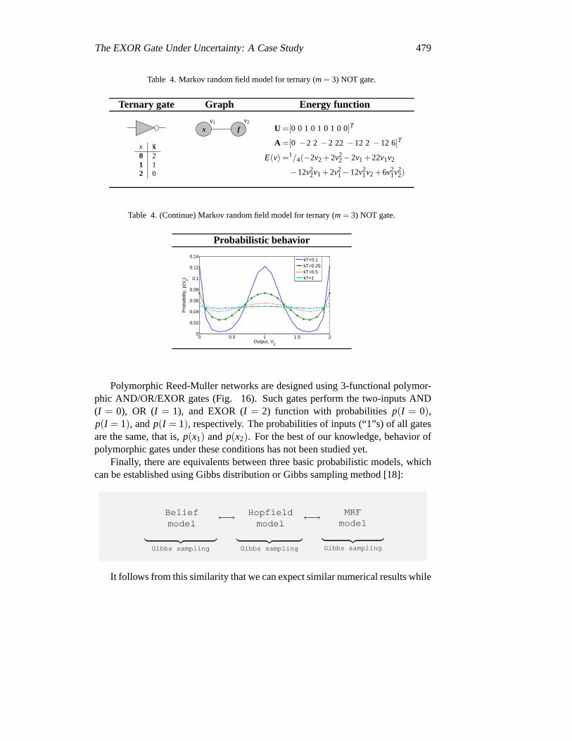
However, multivalued extension of Hopfield-based logic networks is verycom-plicated. In contrast, the MRF model can be easy generalized for multivalued logic.Example is given in Table 4. We used 0-polarity arithmetic transforms for the 3-valued NOT gate [23]. Extension for an arbitrary library of multivalued gates isstraightforward.
Other models of fault-tolerant logic gates exist, for example,polymorphicgatesfor sensor-based systems [26]. Polymorphic gate is a multi-functional logicdevicethat performs logic functionf j , j = 1,2, . . . ,m, if its control input is activated byvalueI j of the signal. In particular, 2-function polymorphic gate is defined as fol-lows:
2-function gate=
{f1, if I1 control value;f2, if I2 control value.
The EXOR Gate Under Uncertainty: A Case Study 479
Table 4. Markov random field model for ternary (m= 3) NOT gate.
Ternary gate Graph Energy function
x x0 21 12 0
f x
v1 v2
U =[0 0 1 0 1 0 1 0 0]T
A =[0 −2 2 −2 22 −12 2 −12 6]T
E(v) =1/4(−2v2 +2v22−2v1 +22v1v2
−12v22v1 +2v2
1−12v21v2 +6v2
1v22)
Table 4. (Continue) Markov random field model for ternary (m= 3) NOT gate.
Probabilistic behavior
0 0.5 1 1.5 20
0.02
0.04
0.06
0.08
0.1
0.12
0.14
Output, V2
Pro
babi
lity,
p(V
2)
kT=0.1kT=0.25kT=0.5kT=1
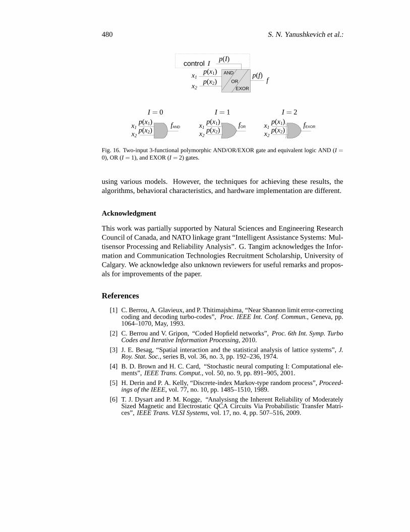
Polymorphic Reed-Muller networks are designed using 3-functional polymor-phic AND/OR/EXOR gates (Fig. 16). Such gates perform the two-inputs AND(I = 0), OR (I = 1), and EXOR (I = 2) function with probabilitiesp(I = 0),p(I = 1), andp(I = 1), respectively. The probabilities of inputs (“1”s) of all gatesare the same, that is,p(x1) andp(x2). For the best of our knowledge, behavior ofpolymorphic gates under these conditions has not been studied yet.
Finally, there are equivalents between three basic probabilistic models, whichcan be established using Gibbs distribution or Gibbs sampling method [18]:
Beliefmodel
︸ ︷︷ ︸
Gibbs sampling
←→Hopfieldmodel
︸ ︷︷ ︸
Gibbs sampling
←→MRF
model
︸ ︷︷ ︸
Gibbs sampling
It follows from this similarity that we can expect similar numerical results while
480 S. N. Yanushkevich et al.:
x1
x2 f
AND
OR
I
p(f)
p(I)
p(x1)
p(x2)
control
EXOR
I = 0
x1
x2
fAND p(x1) p(x2)
I = 1
x1
x2
fOR p(x1) p(x2)
I = 2
x1
x2
fEXOR p(x1) p(x2)
Fig. 16. Two-input 3-functional polymorphic AND/OR/EXOR gate and equivalent logic AND (I =0), OR (I = 1), and EXOR (I = 2) gates.
using various models. However, the techniques for achieving these results, thealgorithms, behavioral characteristics, and hardware implementation are different.
Acknowledgment
This work was partially supported by Natural Sciences and Engineering ResearchCouncil of Canada, and NATO linkage grant “Intelligent Assistance Systems: Mul-tisensor Processing and Reliability Analysis”. G. Tangim acknowledges theInfor-mation and Communication Technologies Recruitment Scholarship, University ofCalgary. We acknowledge also unknown reviewers for useful remarks and propos-als for improvements of the paper.
References
[1] C. Berrou, A. Glavieux, and P. Thitimajshima, “Near Shannon limit error-correctingcoding and decoding turbo-codes”,Proc. IEEE Int. Conf. Commun.,Geneva, pp.1064–1070, May, 1993.
[2] C. Berrou and V. Gripon, “Coded Hopfield networks”,Proc. 6th Int. Symp. TurboCodes and Iterative Information Processing, 2010.
[3] J. E. Besag, “Spatial interaction and the statistical analysis of lattice systems”,J.Roy. Stat. Soc.,series B, vol. 36, no. 3, pp. 192–236, 1974.
[4] B. D. Brown and H. C. Card, “Stochastic neural computing I: Computational ele-ments”, IEEE Trans. Comput., vol. 50, no. 9, pp. 891–905, 2001.
[5] H. Derin and P. A. Kelly, “Discrete-index Markov-type random process”,Proceed-ings of the IEEE, vol. 77, no. 10, pp. 1485–1510, 1989.
[6] T. J. Dysart and P. M. Kogge, “Analysisng the Inherent Reliability of ModeratelySized Magnetic and Electrostatic QCA Circuits Via Probabilistic Transfer Matri-ces”, IEEE Trans. VLSI Systems, vol. 17, no. 4, pp. 507–516, 2009.

The EXOR Gate Under Uncertainty: A Case Study 481
[7] S. T. Chakradhar, V. D. Agrawal, and M. L. Bushnell, Neural Models and Algo-rithms for Digital Testing. Kluwer, Dordrecht, 1991.
[8] B. R. Gaines, “Stochastic computing systems”, in “Advances in Information Sys-tems Science”, J. T. Tou, Ed., Plenum, New York, vol. 2, chap.2, pp. 37–172, 1969.
[9] J. J. Hopfield, “Neural networks and physical systems with emergent collectivecomputational abilities”,Proceedings of National Academy of Sciences, USA, vol.79, pp. 2554–2558, 1982.
[10] S. E. Lyshevski, S. N. Yanushkevich, V. P. Shmerko, et al., “Computing Paradigmsfor Logic Nanocells.”,J. Computational and Theoretical Nanoscience, vol. 5, pp.2377–2395, 2008.
[11] S. E. Lyshevski, V. P. Shmerko, M. A. Lyshevski, et al., “Neuronal processing,reconfigurable neural networks and stochastic computing”,Proc. IEEE Conf. Nan-otechnology, Arlington, TX, 2008.
[12] H.-A. Loeliger, F. Lustenberger, M. Helfenstein, et al., “Probability propagationand decoding in analog VLSI”,IEEE Trans. Inf. Theory,vol.47, no.2, pp.837–843,2001.
[13] C. Mead, “Neuromorphic electronic systems”,Proc. IEEE, vol. 78, no 10, pp.1629–1639, 1990.
[14] C. L. Janer, J. M. Quero, J. G. Ortega, et al., “Fully parallel stochastic computationarchitecture”,IEEE Trans. Signal Processing, vol. 44, no. 8, pp. 2110–2117, 1996.
[15] F. V. Jensen,Bayesian Networks and Decision Graphs,Springer, 2001.
[16] A. A. Mullin, “Stochastic combinational relay switching circuits and reliability”,IRE Trans. Circuit Theory, vol. 6, no. 1, pp. 131–133, 1959.
[17] A. F. Murray and A. V. W. Smith, “Asynchronous VLSI neural networks usingpulse-stream arithmetic”,IEEE J. of Solid, vol. 23, no. 3, pp. 688–697, 1988.
[18] P. Myllymaki, “Using Bayesian networks for incoporating probabilistic a prioryknowledge into Boltzmann machines”,Proc. SOUTH Conf., pp. 97–102, Orlando,1994.
[19] K. Nepal, R. I. Bahar, J. Mundy, W. R. Patterson, et al., “Designing NanoscaleLogic Circuits Based on Markov Random Fields”,J. Electronic Testing: Theoryand Applications, vol. 23, pp. 255–266, 2007.
[20] K. P. Parker and E. J. McCluskey, “Probabilistic treatment of general combinationalnetworks”, IEEE Trans. Comput., vol. 24, no. 6, pp. 668–670, 1981.
[21] U. Kalay, D. V. Hall, and M. A. Perkowski, “A minimal universal test set for self-test of EXOR-sum-of-products circuits”,IEEE Trans. on Comput., Vol. 49, Issue 3,pp. 267 - 276, 2000.
[22] P. W. K. Rothemund, N. Paradakis, and E. Winfree, “Algorithmic self-assembly ofDNA Sierpinski triangles”, PloS Biology — www.plosbiology.org, vol.2, issue 12,e424, pp. 2041–2053, 2004.
[23] V. P. Shmerko, S. N. Yanushkevich, and S. E. Lyshevski,Computer Arithmetics forNanoelectronics, Taylor & Francis/CRC Press, Boca Raton, FL, 2009.
[24] S. Shukla and R. I. Bahar (Eds.), “Nano, Quantum and Molecular Computing: Im-plications to High Level Design and Validation”, Kluwer, 2004.
[25] S. Stankovic and J. Astola, “Representation of Resilient Boolean Functions UsingBinary Decision Diagrams”,Proc. Reed-Muller 2011 Workshop, Tuusula, Finland,pp. 93-98, May 2011.

482 S. N. Yanushkevich et al.:
[26] A. Stoica, R. Zebulum, and D. Keymeulen, “Polymorphic electronics”, Proc. 4thInt. Conf. Evolvable systems: from biology to hardware, Tokyo, Japan, 2001, pp.291-001.
[27] A. H. Tran, S. N. Yanushkevich, S. E. Lyshevski, et al. “Fault Tolerant Comput-ing Paradigm for Random Molecular Phenomena: Hopfield Gatesand Logic Net-works”, IEEE Int. Symp. Multi-Valued Logic, pp. 93 - 98, 2011.
[28] D. E. Van Den Bout and T. K. Miller III, “A digital architecture employingstochastism for the simulation of Hopfield neural nets”,IEEE Trans. Circuits andSyst., vol. 36, no. 5, pp. 32–738, 1989.
[29] S. N. Yanushkevich and V. P. Shmerko, “Teaching Reed-Muller techniques in intro-ductory classes on logic design”,FACTA Universitatis., ser. Elec. Energ., vol. 20,no. 3, pp. 331–065, 2007.
[30] S. N. Yanushkevich, A. Stoica, and V. P. Shmerko, “Experience of design and pro-totyping of a multi-biometric early warning physical access control security system(PASS) and a training system (T-PASS)”,Proc. 32nd Annual IEEE Industrial Elec-tronics Society Conf.,Paris, 2006.
[31] I-C. Wey, Y-G. Chen, C-H Yu, et al., “Design and Implementation of Cost-EffectiveProbabilistic-Based Noise-Tolerant VLSI Circuits”,IEEE Trans. Circuits and Syst.,vol. 56, no. 11, pp. 2411–2424, 2009.