May 10, 2001

The Fable of the Bees Revisited:Causes and Consequences of the U.S. Honey Program

Mary K. MuthResearch Triangle Institute

Randal R. RuckerMontana State University

Walter N. ThurmanNorth Carolina State University

Ching-Ta ChuangNational Taiwan Ocean University

Abstract: In his 1973 paper, Steven Cheung discredited the “fable of the bees” by demonstrating thatmarkets for beekeeping services exist and that they function well. Although economists heededCheung’s lessons, policy makers did not. The honey program—the stated purpose of which was topromote the availability of pollination services—operated for almost 50 years, supporting the price ofhoney through a variety of mechanisms. Its effects were minor before the 1980s but then becameimportant with annual government expenditures near $100 million for several years. Reforms of theprogram in the late 1980s reduced its market effects and budget costs, returning it to its original role asa minor commodity program. The 1996 Farm Bill formally eliminated the honey program, whichredirected lobbying efforts toward enacting trade restrictions and obtaining annual relief through theappropriations process. We measure the historical welfare effects of the program during its various

incarnations, examine its frequently stated public interest rationale—the encouragement of honeybeepollination, and interpret its history in light of economic theories of regulation.

1The term “fable of the bees” refers to earlier work by Mandeville (1705), which was not connected withexternalities.

The Fable of the Bees Revisited: Causes and Consequences of the U.S. Honey Program

“It has been said that if one dies and goes to heaven and wants to come back to Earth and have eternal life, come back as a federal program”

Rep. Harris W. Fawell (R-Ill, House of Representatives, August 6, 1993).

I. Introduction

In 1973, Steven Cheung recounted the history to that time of what he termed “the fable of the

bees” in economic thought.1 Earlier writers (Meade, 1952; Bator, 1958) had used beekeeping and

apple farming as examples of reciprocal externalities: apple blossom nectar provides food for bees and

the foraging activity of bees pollinates apple blossoms. By stipulating that apple farmers and

beekeepers do not transact, Meade and Bator inferred that the pair of externalities resulted in an

underprovision of both apples and honey.

Cheung’s central point was that the stipulated facts of Meade and Bator’s story, and therefore

the claim of externalities, are fictional—there are well-developed markets in which beekeepers and

growers of crops transact regularly. Arguably, his most persuasive piece of evidence that

interdependencies have been internalized through market transactions is his observation that one needs

only open the Yellow Pages of the phone book in certain Washington towns and find listings there for

pollination services. He went on to analyze data from a small number of beekeepers and concluded

that the markets for pollination services function well: that observed fees reflect both the pollination

value of the bees’ activities and the nectar value of the pollinated crop.

2

While Cheung’s analysis of Washington beekeeping did not disprove the existence of

externalities in other situations, it did sound a caution against the use of blackboard economics for

policy analysis. He illustrated a central point of Coase’s celebrated 1960 paper: that the transaction

costs of market exchange determine the existence and extent of externalities and that to understand

transaction costs (hence externalities) one must understand the institutional details of the market under

consideration.

However, while Cheung may have discredited the bees-and-apples example to the satisfaction

of certain academic economists, his influence did not spread to policy makers. At the time Cheung

wrote, there existed a real policy counterpart to the externality argument, namely the U.S. honey price

support program. Its specific purpose, according to its legislative history, was to promote the

production of pollination on the grounds that markets underprovide such services. (Interestingly,

pollination services were not subsidized, as one might propose from the blackboard. Rather, the price

of its complementary output—honey—was supported.) Cheung was aware of the program and

correctly argued that it had minimal influence at the time. In the 30 years since he wrote, however, the

honey program has had major effects in honey and pollination markets and, for a relatively minor

commodity, has generated substantial government expenses. Largely as a result of these expenses, the

honey program was eliminated in the 1996 Farm Bill. Since then, honey producers have successfully

lobbied for other forms of support through trade restrictions and through the annual appropriations

process.

An analysis of this program—its causes and effects from cradle to grave and beyond—is the

focus of our paper. With respect to the causes of the honey program, the fact that it has gone through a

3

2Previous work has addressed aspects of the honey program. Willett and French (1991) and Smargiassi andWillett (1989) considered the effects of the support program on honey producers, but neither measured explicitly theprogram’s welfare effects or studied its political economy. Our analysis, which extends work by Chuang (1992), doesboth.

3For seminal articles in this literature, see Stigler (1971), Peltzman (1976), and Becker (1983). For applications tofarm subsidies, see Gardner (1987) and Rucker and Thurman (1990).

complete birth-to-death cycle makes it relatively unique among long-lived U.S. commodity programs.

Lessons learned from it should prove useful for understanding aspects of other programs. With respect

to its effects, we find the usual commodity program distortions in the honey market—taxpayers lose and

a relatively small number of commercial beekeepers obtain substantial gains (between $10,000 and

$20,000 annually per participating producer) for a brief period in the 1980s. Interestingly, we find that

domestic consumers also benefitted from the program.2

Widely accepted economic models of regulators’ behavior hold that for a given industry, a

political equilibrium will be established that balances at the margin the competing interests of consumers,

producers, and taxpayers.3 Shocks to the industry of various sorts can induce adjustments to a new

political equilibrium. Below we recount and interpret the history of the honey program from the

perspective of such a political economic model. We conclude that the underlying political equilibrium of

support for beekeeping is a stable one. The post-World War II history of the industry is characterized

by short periods of out-of-equilibrium levels of support, followed by the re-institution in various guises

of a modest subsidy.

The paper proceeds as follows. In Section II, a model of the honey program is presented in

which the history of the support program is interpreted. A welfare accounting follows, considering the

effects of policy on both honey and pollination markets. Section III examines the political economy of

4

4See Hoff and Willett (1994) for a detailed description of the program and its history. A packer purchase programthat operated in 1950 and 1951 is not shown here, but we describe its operation in Section III.

the program. In Section IV, we summarize our findings and draw a connection between the political

economy literature and work by Barzel that accentuates the seemingly limitless number of margins for

adjustment to changing conditions in non-political market settings.

II. The Honey Program: History and Economic Effects

We first develop a model of the U.S. honey market, recounting the effects of the honey support

program from 1952 through 1993. We then use the framework for estimating consumer and producer

benefits and taxpayer expenses and consider the indirect effects of the honey program on markets for

pollination.

II.A. A Model of the Honey Program’s Effects on Honey Markets

The methods by which honey producers participated in the honey support program evolved

over time. We represent the three primary regimes in figure 1.4 During the first, from 1952 to 1979,

the honey program was a standard commodity price support program (see Pasour, 1990). Producers

could place their honey under loan at a support price and then either forfeit the honey to the

government, keeping the original loan proceeds, or redeem the honey to sell it on the market (paying

back the loan plus interest). During this time the world price of honey, PW (assumed here to be

exogenous), was above the support price, PS. Producers had no incentive to forfeit their honey, and

the government costs of running the program amounted to administration costs and an interest rate

subsidy.

5

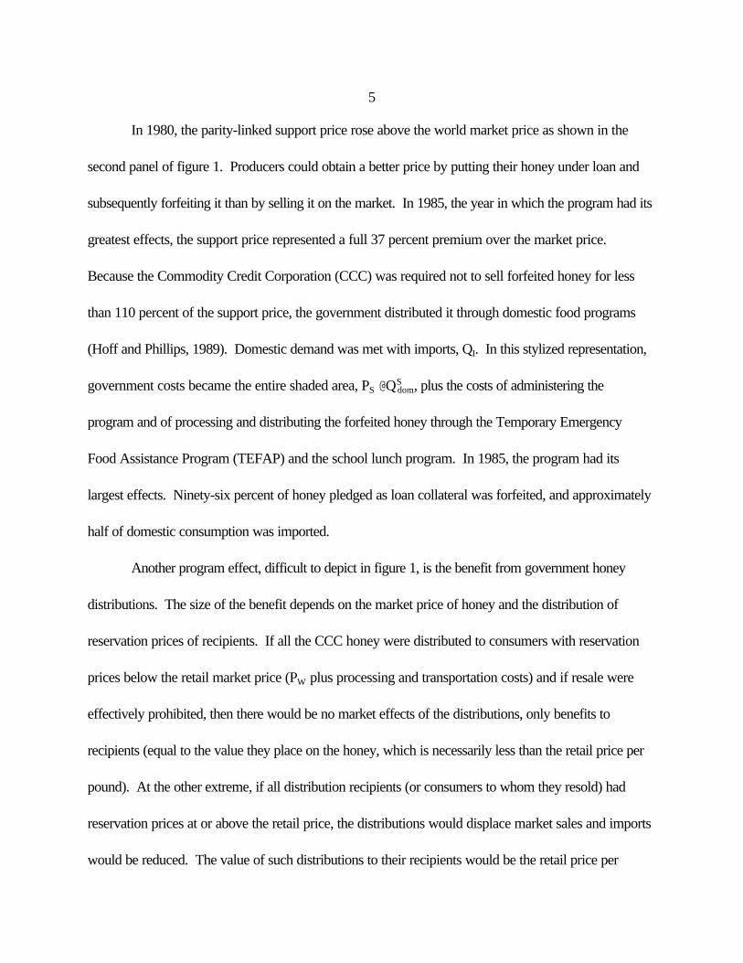
In 1980, the parity-linked support price rose above the world market price as shown in the

second panel of figure 1. Producers could obtain a better price by putting their honey under loan and

subsequently forfeiting it than by selling it on the market. In 1985, the year in which the program had its

greatest effects, the support price represented a full 37 percent premium over the market price.

Because the Commodity Credit Corporation (CCC) was required not to sell forfeited honey for less

than 110 percent of the support price, the government distributed it through domestic food programs

(Hoff and Phillips, 1989). Domestic demand was met with imports, QI. In this stylized representation,

government costs became the entire shaded area, PS @ QSdom, plus the costs of administering the

program and of processing and distributing the forfeited honey through the Temporary Emergency

Food Assistance Program (TEFAP) and the school lunch program. In 1985, the program had its

largest effects. Ninety-six percent of honey pledged as loan collateral was forfeited, and approximately

half of domestic consumption was imported.

Another program effect, difficult to depict in figure 1, is the benefit from government honey

distributions. The size of the benefit depends on the market price of honey and the distribution of

reservation prices of recipients. If all the CCC honey were distributed to consumers with reservation

prices below the retail market price (PW plus processing and transportation costs) and if resale were

effectively prohibited, then there would be no market effects of the distributions, only benefits to

recipients (equal to the value they place on the honey, which is necessarily less than the retail price per

pound). At the other extreme, if all distribution recipients (or consumers to whom they resold) had

reservation prices at or above the retail price, the distributions would displace market sales and imports

would be reduced. The value of such distributions to their recipients would be the retail price per

6

5Depending on the mechanisms by which free honey was distributed, the dissipation of the value of the freegood, and hence the welfare costs of the program, could be substantially understated. Systematic information onhoney distribution procedures is hard to come by because free food distribution programs were administered locally. A 1988 article from the Los Angeles Times gives an anecdotal account of the costs of free food distribution. Thearticle describes how the San Diego Food Bank distributed limited supplies of federal food—cheese, butter, dry milk,cornmeal, flour, and rice—in addition to honey:

“At one distribution site Friday, more than 400 people picked up allotments of butter, flour, milk andcornmeal.... Some arrived as early as 6 a.m. to be among the first in line for an 8 a.m. opening at Our Lady ofMt. Caramel Church in Rancho Penasquitos.

Debbie Johnston, a housewife and mother of three children, said she doesn’t mind standing in line so longbefore the distribution site opens each month if it means she can pick up items her family might otherwisehave to do without ... With two of her children in tow, Johnston was one of the first people in line, whichstretched midway into the church’s parking lot at one point. As she made her way through the churchdoors, picked up her family’s allocation of commodities—estimated to be worth about $10 at marketvalue—and headed to her car, hundreds of other people waited for their turn.” (“Shortages Hit Distributionof Surplus Foods,” Los Angeles Times, San Diego County Edition, 9/28/88) Note that if Ms. Johnston’sopportunity cost of time were $5 per hour, the value of her allocation was totally dissipated.

pound—the savings from replacing market purchases with distributions. But further, some or even all

of the value to recipients can be dissipated by the process of distribution. If distribution of free honey

entails queuing, then a portion of the value of the distributed honey will be dissipated and waiting time

costs should be counted among the resource costs of the program (see Barzel, 1974 and 1989, ch. 2).

In what follows, and due to the absence of appropriate data, we assume that queuing costs are zero

and base our welfare change estimates on that assumption, recognizing that this biases downward our

estimates of the program’s costs.5

The large market effects in the early 1980s were addressed by legislative modifications to the

program. Beginning with the 1986 crop year, Congress altered the honey program by dropping the

parity-based formula, setting a sequence of progressively lower support prices, and allowing for a

marketing loan option. In the third panel of figure 1, producers placed their honey under loan at the

support price, PS, and later redeemed it at the repayment rate, PR, in order to sell it at the world price,

7

PW. Producers who sold their honey on the market at PW received a subsidy equal to the difference

between the support price and the repayment rate. The per pound subsidy, PS ! PR, ranged from a

high of 23 cents in 1986 to a low of 5.9 cents in 1991. Government costs under the 1986 revisions

are represented by the shaded area (PS ! PR) @ QSdom. In addition, the government costs of processing

and distributing forfeited honey were reduced because producers forfeited less honey. Although it

appears that producers had little incentive to forfeit honey pledged as loan collateral, many continued to

do so, especially for the first couple of years after the program was altered. However, by 1992 only

2.8 percent of honey pledged as collateral was forfeited. Further alterations in the program for 1991

through 1993 allowed producers to receive a direct subsidy equal to PS ! PR without the pretense of

putting their honey under loan. These subsidies are also represented in the third panel of figure 1.

In late 1993, Congress reauthorized the program through 1998, but the 1994 and 1995

Appropriations Acts eliminated government expenditures for each of those fiscal years (see Hoff,

1995). When the Appropriations Committee chose not to fund the honey support program for 1994

and 1995, it no longer was possible for producers to forfeit honey pledged as collateral or to receive

payments of the difference between the support price and the repayment rate. During these years,

honey loans were loans in the ordinary sense; producers had to repay the loan proceeds with accrued

interest, and the honey program had little effect.

The honey program was eliminated in the 1996 Farm Bill. Since then, the domestic subsidy to

honey production has consisted largely of loans made to beekeepers at below-market interest rates.

Trade actions against honey imports from China, however, have also borne fruit. Most recently, the

8

6See Public Law 106-387, Section 812. These relief tools are essentially the same as those used for the honeyprogram between 1990 and 1993. A notable distinction is that the 2000 legislation only specifies payments for oneyear.

7Arguably, the price of the other primary beekeeping output, pollination services, should also be included in acolony response equation. We do not include such an effect for two reasons. First, pollination fees vary greatly bylocation and crop. Unlike honey, for which a national market exists, pollination fee data are intrinsically local and nosuitable national series exists. Second, we do not want to measure the welfare effects of changes in honey priceswith pollination fees held constant. Instead, we would like to measure the effects to all beneficiaries of a honey priceincrease. If, as we argue later, honey price support lowers equilibrium pollination fees, then the beneficiaries includefarmers who purchase pollination services. If variations in honey price are econometrically exogenous in our honeysupply equation, then the equation has a general equilibrium interpretation. Measured producer surplus changesinclude welfare gains to the beneficiaries of lower pollination fees (see Harberger, 1971, and Thurman, 1991).

essence of the early 1990's honey program was revived when appropriations were made for marketing

assistance loans and loan deficiency payments for the year 2000 crop of honey.6

II.B. Welfare Accounting in Honey Markets

Effects on Beekeepers

To estimate the effects of the honey program on beekeepers, we model the supply of honey in

the United States assuming that the stock of colonies maintained by U.S. beekeepers is affected by the

expected price of honey, other input costs associated with honey production, and costs of adjustment

represented by lagged colonies.7 We then estimate the hypothetical quantity of honey that would have

been supplied without the honey support program.

Expected honey producer prices will be influenced by government policy, which we address

econometrically by estimating expected honey prices differently for each of the phases of the honey

support program. For 1951 through 1980, we generate one-year-ahead expected honey prices from

an autoregressive (AR2) process in first differences. Beginning with 1981 and through the period of

large program effects, we assume that producers based their colony decisions on the support price,

which was known prior to the crop year. For 1986 through 1991, we calculate the expected honey

9

price as the support price plus the average producer price–repayment rate differential. The input cost

index included in the supply response equation is a weighted average of the wage component of prices

paid by farmers and the fuel and container components of the producer price index.

Estimation of the colony response equation is complicated by two limitations to the official

USDA data. The first is that colony numbers were not recorded during the years 1982 to 1985,

although price and cost data are available. The second limitation is that when the National Agricultural

Statistics Service (NASS) began again to collect colony data, it changed its method of data collection.

In the official estimates, the number of colonies dropped dramatically in 1986 by 1 million colonies,

from a prior level of approximately 4 million colonies. Conversations with USDA–NASS employees

confirm that changes were made in how the data are collected. Hoff and Phillips (1989) state that while

earlier estimates included colony counts from all beekeepers, the later years included counts only from

those beekeepers who maintained at least five colonies. In the Appendix, we describe a maximum

likelihood estimation method that enables us to account for the hiatus in data collection in the early

1980s and to parsimoniously estimate the effects of the change in survey methods. Our estimation

strategy parameterizes the change in methods as a one-time reduction in the number of colonies

counted. Our estimate of that reduction is 863,000 colonies with a standard error of 195,000 colonies.

In the welfare accounting that we present in tables 2 and 3, we adjust the official numbers with our

estimated undercount.

The results of the maximum likelihood estimation of the colony supply equation are presented in

table 1. We include the expected honey price and the input cost index in ratio form to impose

homogeneity. The estimated coefficient of 394.3 implies a short-run price elasticity of colony supply,

10

8For each year, we obtain the predicted difference in colony populations from the contemporaneous price effectand a lagged colony effect. We calculate the contemporaneous price effect by multiplying the price coefficient ofthe colony supply equation (394.3) by the difference between the support price and the expected producer price. Next, we calculate the lagged colony effect by multiplying the lagged colony coefficient (0.97) by the previous year’spredicted change in colony population. Because of the lagged colony effect, table 3 shows quantity supplied effectstailing off in 1994 and 1995, but we calculate no producer welfare effects in those years because the program had noeffect on price.

evaluated at the means of the data, of 0.052 and a long-run price elasticity of 2.01. These estimates

can be compared to the short-run and long-run elasticities of 0.024 and 0.242 reported by Willett and

French (1991). The estimates imply that beekeepers adjust the number of colonies slowly in response

to changes in expected producer prices.

To measure the effects of the program on producers, we determine first the level of colony

investment without price support and then multiply the number of predicted colonies by average colony

yields as reported by the USDA to obtain estimates of the hypothetical level of honey production

without the program. The table 1 estimates allow us to generate a dynamic prediction of the change in

colonies due to removing the honey price support.8 In figure 1, the level of production without the

support program corresponds to finding the point where the U.S. supply of honey intersects PW

(point d in the center panel of figure 1 and point i in the right panel of figure 1). The net benefits to

producers from the program are represented by area abcd for the years 1980 through 1985 and area

fghi for the years 1986 through 1993.

In table 2, the predicted reductions in colony populations range from about 6,000 colonies in

1981 (a 0.1 percent reduction) to 451,000 colonies in 1993 (a 12 percent reduction). The associated

predicted reductions in honey production range from 0.3 to 26.9 million pounds.

11

9In figure 1, we portray the supply of honey to the United States as perfectly elastic, but our estimates of domesticproducer benefits do not depend on this assumption. For the 1981 through 1985 period, the import elasticity isirrelevant because producers received the fixed support price. For the 1986 through 1993 period, producers receivedthe support price plus the differential between the world price and the loan repayment rate. Because the repaymentrate was adjusted in response to changes in the world price, the differential was relatively constant and the pricereceived by producers did not depend upon the world price.

Table 3 presents the net producer benefits. For 1981 through 1985, we calculate gross

producer benefits by multiplying honey forfeitures by the difference between the support price and the

producer price. For 1986 through 1990, we add to the value of forfeitures the direct subsidies paid on

honey that was placed under loan and then redeemed. For 1991 through 1993, we include all of the

above plus the value of direct subsidies paid on honey that was not placed under loan. We also

subtract a newly instituted Agricultural Stabilization and Conservation Service (ASCS) assessment of 1

percent of the support price. To obtain the estimates of net producer benefits presented in table 3, we

subtract the deadweight loss triangles, shown in figure 1, which we calculated using the predicted

reductions in production without the support program from table 2. Based on these calculations, net

producer benefits range from $0.3 million in 1981 to a peak of $40.3 million in 1987.9

Effects on Honey Consumers

Under the assumption that variations in net U.S. imports did not influence the world price,

consumers were affected by the honey program only through the distribution of CCC honey stocks.

Consumers who would have purchased honey on the market but instead receive free honey

distributions receive a benefit. Recipients who would not have purchased honey also receive a positive,

but smaller, benefit. Measurement of the welfare effect on consumers depends on measuring this

displacement (see also footnote 7 on the dissipation of value through queuing).

12

10Because a retail honey price was not published for the years 1980 to 1986, we constructed those prices based onthe observed relationship between the producer price and the retail price for the years 1950 through 1979 and 1987through 1992.

To measure the displacement, we hypothesize that domestic consumption of honey is directly

affected by the quantity of CCC distributions and a linear and quadratic time trend. We found in

alternative specifications that the price of honey, the price of its closest substitute (sugar), and income

had statistically insignificant effects and, importantly, their inclusion did not significantly alter the values

of the other estimated coefficients.10 The results of OLS estimation of the consumption equation are

presented in table 1. Of relevance to welfare measurement, CCC honey distributions had a significant

and substantial negative effect on honey consumption. Each additional pound of honey distributed by

the CCC is estimated to decrease per capita consumption of honey at the retail level by 0.76 of a

pound. CCC distributions did not offset per capita retail purchases pound for pound because some

recipients would not otherwise have purchased honey. (However, the CCC distributions coefficient is

not significantly different from –1 at conventional levels.) The linear and quadratic trend coefficients are

also significant and indicate a decreasing trend in honey consumption through 1982 and an increasing

trend thereafter. This trend roughly corresponds with the increased use of honey in processed food

products and, later, promotional efforts by the National Honey Board.

We use the estimated effect of CCC distributions on honey consumption to estimate the benefit

to consumers from the honey support program. We assume that the proportion of each pound of

CCC-distributed honey that offsets honey consumption from market sources is valued by consumers at

the retail price of honey. The remaining proportion of each pound—which goes to consumers who

would not otherwise have purchased this honey—we assume is valued at the lower retail price of sugar

13

11To make the calculations of benefits consistent for producers and consumers, we base the actual consumerbenefit calculations on forfeitures rather than on CCC distributions of honey. Because honey can be stored for a fewyears, CCC distributions lagged forfeitures.

12The calculations of consumer benefits assume that the supply of honey to the United States is perfectly elastic.One justification for this is that the United States imports only about 10 percent of world production. If, however,the supply of honey is upward sloping, our calculations may overstate the benefits to consumers between 1980 and1985 and understate the benefits after 1985. In the 1980 to 1985 period, imports of honey into the United Statesincreased greatly as producers forfeited greater quantities of honey. This effectively shifted out the excess demandfor honey by the United States. With an upward sloping excess supply curve, this would result in a higher worldprice for honey, which would translate into a higher retail price and a loss of surplus to those consumers who wouldhave purchased honey. In addition, the U.S. support program would then have effects on foreign consumers andproducers. Foreign consumers would suffer a loss in surplus and foreign producers would net a gain in surplus as aresult of the higher world price.

From 1986 on the situation is reversed. The relevant supply price to U.S. producers under this regime of thesupport program is the world price plus the support price-repayment rate differential. In this case, more honey ismarketed by U.S. producers and the excess demand for honey by the United States pivots in at the support price. With an upward sloping excess supply curve, the resulting equilibrium world price would decrease. Hence, domesticconsumers who purchase honey on the market would gain in surplus relative to our calculations. Foreign producerswould suffer a loss in surplus and foreign consumer surplus would increase.

as an approximation. The difference between the retail price of honey and the retail price of sugar for

these consumers represents a deadweight loss to society from CCC distributions.11 As shown in table

3, net consumer benefits reached a peak of $78 million in 1983 but declined to less than $1 million by

1990.12

Effects on Taxpayers and Net Benefits to Society

Taxpayers pay the cost of subsidizing beekeepers and distributing donated honey, including the

costs of storage, processing, handling, and transportation. One way to estimate distribution costs is to

use the markup between the retail honey price and the producer price, which was on average 31.2

cents per pound over the 1981 to 1995 period. We estimate the distribution cost component of

taxpayer expense as the product of the average markup and the number of pounds of honey forfeited

by producers. For 1981 through 1985, taxpayer expenses are these distribution costs plus the amount

14

paid to honey producers for forfeited honey. The cost of forfeited honey is represented by area bclk in

the middle panel of figure 1. For 1986 through 1990, taxpayer expenses are the sum of (1) the support

price–repayment rate differential for each pound of honey bought back from the CCC, and (2) the

distribution costs and producer receipts for forfeited honey. For 1991 through 1993, taxpayer

expenses are the costs associated with all of these components, plus the direct subsidy payments of the

support price–repayment rate differential collected on honey not put under loan, and less the 1 percent

ASCS assessment.

The resulting calculated taxpayer expenses are presented in table 3. The deadweight loss as a

result of the program, calculated as net consumer benefits plus net producer benefits minus taxpayer

expenses, also is reported in the last column of table 3. The years with the highest taxpayer expenses in

the early 1980s are associated with the largest net social losses. Alterations in the program as of 1986

reduced both taxpayer expenses and the net social loss. By the late 1980s, the benefits to consumers

and honey producers nearly offset the taxpayer expenses of the honey program.

II.C. The Effects of the Honey Subsidy on Pollination

The effects of the honey program in the honey market are relatively straightforward.

Consumers and producers trade in well-defined markets, and the welfare effects of market

interventions are, in principle, measurable. Less straightforward are the effects of the honey program

on consumers and producers of pollination services.

There are two types of beekeeping situations. There are those where the welfare gains from

contracting between beekeepers and farmers are less than the transaction costs. These are markets

with “pollination externalities”—markets in which increases in pollination services would generate net

15

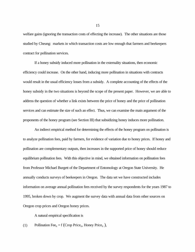
welfare gains (ignoring the transaction costs of effecting the increase). The other situations are those

studied by Cheung: markets in which transaction costs are low enough that farmers and beekeepers

contract for pollination services.

If a honey subsidy induced more pollination in the externality situations, then economic

efficiency could increase. On the other hand, inducing more pollination in situations with contracts

would result in the usual efficiency losses from a subsidy. A complete accounting of the effects of the

honey subsidy in the two situations is beyond the scope of the present paper. However, we are able to

address the question of whether a link exists between the price of honey and the price of pollination

services and can estimate the size of such an effect. Thus, we can examine the main argument of the

proponents of the honey program (see Section III) that subsidizing honey induces more pollination.

An indirect empirical method for determining the effects of the honey program on pollination is

to analyze pollination fees, paid by farmers, for evidence of variation due to honey prices. If honey and

pollination are complementary outputs, then increases in the supported price of honey should reduce

equilibrium pollination fees. With this objective in mind, we obtained information on pollination fees

from Professor Michael Burgett of the Department of Entomology at Oregon State University. He

annually conducts surveys of beekeepers in Oregon. The data set we have constructed includes

information on average annual pollination fees received by the survey respondents for the years 1987 to

1995, broken down by crop. We augment the survey data with annual data from other sources on

Oregon crop prices and Oregon honey prices.

A natural empirical specification is

(1) Pollination Feeit = f (Crop Priceit, Honey Priceit ),

16

13Pollination fees, crop prices, and honey prices are deflated (base year = 1991) for the empirical analysis.

where for crop i in year t, Pollination Feeit is the average pollination fee (in dollars per colony) reported

in the survey; Crop Priceit is the average crop price in Oregon (in dollars per pound); and Honey Priceit

is the average price of honey received by producers in Oregon (in dollars per pound).13

The expected sign of the coefficient on Crop Price is positive—an increase in the price of a

pollinated crop increases the VMP of pollination services, which should increase pollination fees in

equilibrium. We assume an upward sloping supply of bee colonies for annual variations in price. The

sign of the estimated coefficient on Honey Price is a priori ambiguous but is interesting as it provides

insights into the validity of the arguments made by proponents of the honey program. A negative sign is

consistent with the argument that an increase in honey prices increases the number of bees available for

pollination and that this increase in supply of pollination services reduces pollination fees. A positive

sign suggests that an increase in honey prices causes beekeepers to shift more of their colonies from

providing pollination services to producing honey, thereby reducing the supply of pollination services

and increasing pollination fees.

Beekeepers and landowners agree on pollination fees at the time colonies are placed in

orchards and fields, typically in the spring or early summer months. Because the fees are determined

prior to the time that actual crop prices for the year are known, fees must be based on expectations of

what crop prices will be. We use as a proxy for the expected crop price the crop price from the

previous year. Similarly, Oregon honey prices for year t are determined after pollination fees are

specified. In the presence of the honey price support program, however, each year’s honey price

17

14Note that we use the actual average honey price rather than the support price. Given that there were differentsupport prices for different grades of honey and given that support prices were binding during the period of ouranalysis, we assume that the observed average honey price was an appropriately weighted average of the varioussupport prices.

15The survey responses do not include fee information for all of the 11 crops for every year. Our data set iscomprised of the following: 9 observations on pears, sweet cherries, apples, cucumbers, blueberries, and radishseed; 8 observations on vetch seed; 7 observations on crimson clover seed and squash; and 6 observations on redclover seed and cranberries.

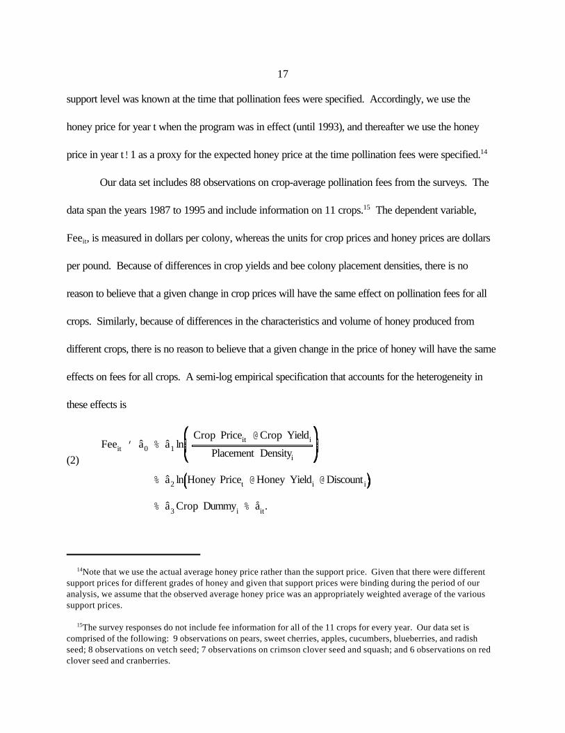
support level was known at the time that pollination fees were specified. Accordingly, we use the

honey price for year t when the program was in effect (until 1993), and thereafter we use the honey

price in year t!1 as a proxy for the expected honey price at the time pollination fees were specified.14

Our data set includes 88 observations on crop-average pollination fees from the surveys. The

data span the years 1987 to 1995 and include information on 11 crops.15 The dependent variable,

Feeit, is measured in dollars per colony, whereas the units for crop prices and honey prices are dollars

per pound. Because of differences in crop yields and bee colony placement densities, there is no

reason to believe that a given change in crop prices will have the same effect on pollination fees for all

crops. Similarly, because of differences in the characteristics and volume of honey produced from

different crops, there is no reason to believe that a given change in the price of honey will have the same

effects on fees for all crops. A semi-log empirical specification that accounts for the heterogeneity in

these effects is

(2)Feeit ' â0 % â1 ln

Crop Priceit @ Crop Yieldi

Placement Densityi

% â2 ln Honey Pricet @ Honey Yieldi @ Discount i

% â3 Crop Dummyi % åit.

18

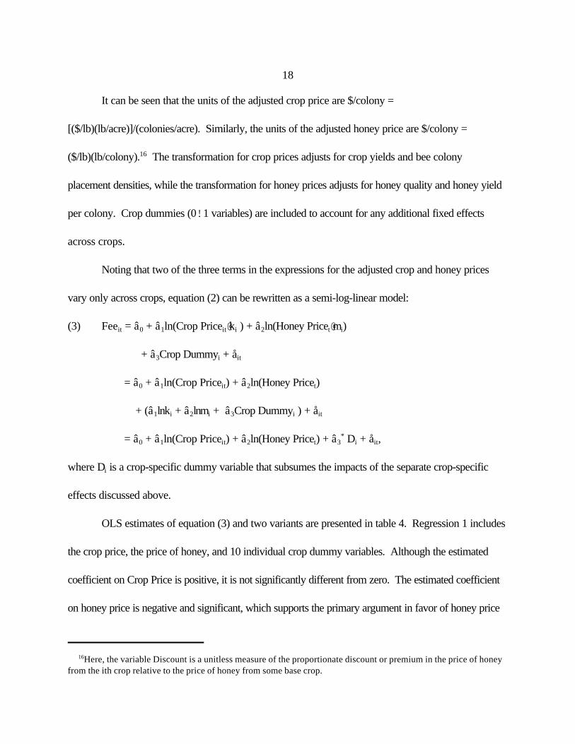
16Here, the variable Discount is a unitless measure of the proportionate discount or premium in the price of honeyfrom the ith crop relative to the price of honey from some base crop.

It can be seen that the units of the adjusted crop price are $/colony =

[($/lb)(lb/acre)]/(colonies/acre). Similarly, the units of the adjusted honey price are $/colony =

($/lb)(lb/colony).16 The transformation for crop prices adjusts for crop yields and bee colony

placement densities, while the transformation for honey prices adjusts for honey quality and honey yield

per colony. Crop dummies (0!1 variables) are included to account for any additional fixed effects

across crops.

Noting that two of the three terms in the expressions for the adjusted crop and honey prices

vary only across crops, equation (2) can be rewritten as a semi-log-linear model:

(3) Feeit = â0 + â1ln(Crop Priceit@ki ) + â2ln(Honey Pricet@mi)

+ â3Crop Dummyi + åit

= â0 + â1ln(Crop Priceit) + â2ln(Honey Pricet)

+ (â1lnki + â2lnmi + â3Crop Dummyi ) + åit

= â0 + â1ln(Crop Priceit) + â2ln(Honey Pricet) + â3* Di + åit,

where Di is a crop-specific dummy variable that subsumes the impacts of the separate crop-specific

effects discussed above.

OLS estimates of equation (3) and two variants are presented in table 4. Regression 1 includes

the crop price, the price of honey, and 10 individual crop dummy variables. Although the estimated

coefficient on Crop Price is positive, it is not significantly different from zero. The estimated coefficient

on honey price is negative and significant, which supports the primary argument in favor of honey price

19

17The only three crop dummy variables whose estimated coefficients are individually significantly different fromzero are those for red and crimson clover seed and vetch seed. The estimated coefficients for all three of these arenegative. Squash is the omitted category.

18Crops that are designated as honey producing crops are vegetable seed, red clover seed, crimson clover seed,vetch seed, raspberries, blueberries, and radish seed.

19Across all crops and years, the average pollination fee is $17.66. For crops that do not produce honey, theaverage fee is $22.96, compared to $11.00 for crops that do produce honey.

support: that an increase in the price of honey increases the availability of pollination services, thereby

driving down pollination fees. The crop dummy variables are jointly significant.17

With a full set of crop dummies, the crop price variable represents only the effects from time

series price variation. It cannot represent the possible effects of inter-crop variation in value. To

examine such an effect, regression 2 replaces the individual crop dummy variables with a 0–1 dummy

variable that is assigned a value of one if honey typically is produced when colonies are placed with the

crop.18 Because beekeepers earn revenues from the honey produced, the fees charged for placing

colonies with these crops are predicted to be less than for crops that yield no income to the beekeeper.

Thus, we predict a negative estimated coefficient for the Honey Crop variable. As can be seen from

table 4, this prediction is borne out by the highly significant coefficient on this variable. Further, the

estimated coefficient on the Crop Price variable becomes positive and significant, and the coefficient on

Honey Price remains negative and significant. The coefficient on the Honey Crop variable suggests that

the pollination fee for crops that produce honey is about $17 per colony less than for crops that

produce no honey.19 The results also suggest that a 10 percent increase in average honey prices causes

a decrease in pollination fees of about $2.50 per colony and that a 10 percent increase in crop prices

causes an increase in pollination fees of about $0.40 per colony.

20

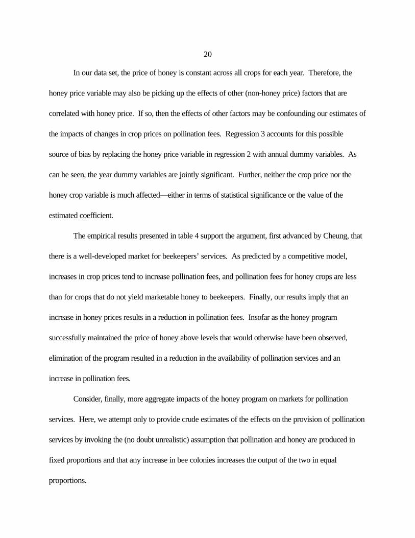
In our data set, the price of honey is constant across all crops for each year. Therefore, the

honey price variable may also be picking up the effects of other (non-honey price) factors that are

correlated with honey price. If so, then the effects of other factors may be confounding our estimates of

the impacts of changes in crop prices on pollination fees. Regression 3 accounts for this possible

source of bias by replacing the honey price variable in regression 2 with annual dummy variables. As

can be seen, the year dummy variables are jointly significant. Further, neither the crop price nor the

honey crop variable is much affected—either in terms of statistical significance or the value of the

estimated coefficient.

The empirical results presented in table 4 support the argument, first advanced by Cheung, that

there is a well-developed market for beekeepers’ services. As predicted by a competitive model,

increases in crop prices tend to increase pollination fees, and pollination fees for honey crops are less

than for crops that do not yield marketable honey to beekeepers. Finally, our results imply that an

increase in honey prices results in a reduction in pollination fees. Insofar as the honey program

successfully maintained the price of honey above levels that would otherwise have been observed,

elimination of the program resulted in a reduction in the availability of pollination services and an

increase in pollination fees.

Consider, finally, more aggregate impacts of the honey program on markets for pollination

services. Here, we attempt only to provide crude estimates of the effects on the provision of pollination

services by invoking the (no doubt unrealistic) assumption that pollination and honey are produced in

fixed proportions and that any increase in bee colonies increases the output of the two in equal

proportions.

21

20For seminal articles in this literature, see Stigler (1971), Peltzman (1976), and Becker (1983).

Table 3 reports our econometric estimates of the year-by-year changes in bee colonies induced

by honey price support. Due mainly to lagged adjustment, the largest absolute and proportionate

predicted changes occur late in our simulation period of 1981 to 1991. In 1981, our counterfactual

predicted decline in colony numbers absent the honey program is only one-tenth of a percent. By

1991, our predicted decline is over 6 percent. The fixed proportion assumption implies then that,

absent the honey program, pollination services would have been below actual levels by the same

percentages. Further, in 1991 the program raised the price of honey by 11 percent (see table 2). The

pollination fee regressions in table 4 imply that without the program, pollination fees would have been

about $3 higher.

III. The Political Economy of the Honey Program

Economic models of regulation suggest that for a given industry, a political equilibrium will be

established that balances at the margin competing interests of consumers, producers, and taxpayers.20

Shocks to the industry result in adjustments to a new political equilibrium. Below we recount and

interpret the history of the honey program from the perspective of such a model.

To date, there have been four life stages to the honey program. The birth of the program in the

early 1950s established a political equilibrium in which unrealized public pollination benefits were used

to justify the establishment of a relatively modest subsidy. The second stage was the mid-life crisis in

the 1980s in which events exogenous to the honey industry threw the political market out of equilibrium.

The market was re-equilibrated fairly quickly with subsequent changes to the program. The death of

22

the program came when the modest size of the beekeeping and honey industries, coupled with the

quaint public image of beekeeping, made the honey program a vulnerable political target. Important

factors in the demise of the program included a political climate critical of costly agricultural programs

and the geographic diversity of honey producers—they likely comprised an important constituent in

few, if any, politicians’ districts. Gardner (1987) argues that geographic concentration leads to greater

political support. The fourth (and current) stage of the honey program is the re-establishment of the

modest equilibrium level of support that prevailed from 1950 to 1980 but in the form of trade

restrictions and, most recently, marketing assistance loans and loan deficiency payments for the year

2000 crop.

Stage 1: Birth and Modest Support

The impetus for lobbying for honey price supports in the late 1940s came from two sources.

First, following the end of World War II there was a decline in the demand for honey that caused honey

prices to fall and, it was claimed, threatened to drive beekeepers out of business. Second, there was a

problem producing sufficient legume seed to meet the increased demand for cover crops as farmers

attempted to replenish soil nitrogen levels following World War II. Elaboration on each of these factors

follows.

During World War II, a high national priority was placed on the production of honey (as a

substitute for sugar) and beeswax (which was used for waterproofing military equipment) and also on

assuring an ample stock of bees for pollination of agricultural crops (U.S. Congress, House, 1949, p.

23

21In nominal terms, the average honey price (a weighted average of prices received by producers in wholesale andretail sales) fell by about 35 percent, while the honey producer price (the price received by producers for honey in 60-pound containers) appears to have fallen by about 50 percent (see table 5). Prices in 1949 were still considerablyhigher than they had been prior to the war.

22Statements in the 1949 subcommittee hearings regarding the importance of pollination and the role of honeybeesincluded claims that 80 percent of pollination was accomplished by honeybees (pp. 2, 6, 10, 11, 14, 16), that more than50 agricultural crops relied on pollination (p. 6), and that the value of pollination was 10 to 50 times the value ofhoney (p. 16).

2). Following the war, with the increased availability and falling price of sugar, the demand for honey

fell and the price of honey decreased dramatically between 1947 and 1949 (figure 2).21

Pleas for government price supports at a subcommittee hearing in April 1949 were based in

part on the hardships being borne by beekeepers who claimed to be unable to sell their honey for a

price that covered their costs of production. To a much greater extent, however, the pleas for support

were based on the damage to agriculture that would result from reductions in the pollination services if

substantial numbers of beekeepers failed. Experts who were asked to make the comparison all claimed

that the pollination services were much more valuable than the honey produced.22

At the time, soil nitrogen levels were widely depleted because during WWII farmers had

plowed up fields of nitrogen-replacing crops (clover, vetch, and alfalfa) to replace them with more

profitable nitrogen-depleting crops (tomatoes, sugar beets, corn, and cotton). After the war, farmers

looking to replenish their soil nitrogen levels found that legume seeds were in short supply. The supply

of imports was low because of high post-war demand in Europe. Further, although legume seed prices

were relatively high, yields were not high enough to make significant expanded domestic seed

production profitable.

24

The limited supply of legume seeds also resulted from a reduction in wild bee populations,

which was attributable to the use of new insecticides, the destruction of wild bee habitat, and the

drainage and burning of fence rows as new lands were brought into production. Because wild bees had

previously performed the pollination task with no involvement from farmers, farmers did not

immediately appreciate the importance of the decline.

Research in California in the late 1940s and early 1950s alleviated the dearth of legume seeds.

Prior to this time, the potential contribution of honeybees to seed production had not been realized, and

it appears that farmers were generally not willing to pay pollination fees for legume seeds. In 1949,

however, an innovative beekeeper and an adventuresome farmer—with support from researchers at the

University of California–Davis—demonstrated that intensive use of bees (five hives, rather than one or

two, per acre) increased yields dramatically (roughly 1,000 pounds per acre compared to state average

yields of about 220 pounds). Contemporary accounts of these events (Whitcombe, 1955), as well as

more recent academic research (Olmstead and Wooten, 1987), indicate that although both the

innovative beekeeper and farmer made short-run rents, markets adjusted very quickly to this news.

The supply of pollination services increased quickly, pollination fees rapidly adjusted to a competitive

level, and legume seed prices fell. Thus, it appears that legislative testimony in the late 1940s was

largely accurate regarding shortages of seed supplies, unwillingness of farmers to pay pollination fees for

legume seed production, and falling honey prices.

Given that the major focus of legislative testimony was on problems of pollination, a natural

question is why discussion centered on supporting the price of honey rather than on directly subsidizing

pollination services. While most testimony concerned honey supports, there was some discussion in the

25

23See, for example, the testimony of J. H. Davis from Arkansas and W. T. Gran from Ohio (U.S. Congress, 1949).

24There are few examples of government programs that provide farmers with direct per unit subsidy payments fortheir production activities. A plausible explanation that has been offered for not observing simple direct subsidypayments is that the transfer to farmers and the costs to taxpayers/consumers is too apparent (see Tullock, 1989;Magee, Brock, and Young, 1989; Antle and Johnson, 1990; Rucker, 1995). With price supports, quotas, and targetprice programs, the actual magnitude of the transfer to producers is more difficult to evaluate. The direct lump sumsubsidy payments implemented in the 1996 Farm Bill present a puzzle in this context.

25Hoff and Willett (1994, pp. 56-57) is the primary source of information on the early years of the honey program. The honey program also included export payments and payments for diverting honey to new uses in the early years. Exports averaged about 20 million pounds annually for the 5 years the export payments were in effect. The diversioncomponent of the program had little impact and was abandoned in 1954.

April 1949 hearings of possible pollination subsidy programs.23 Problems with pilot programs in Ohio

and Arkansas concerned the issue of whether to pay the subsidy to the landowner or to the beekeeper

and how to assure that the services claimed had indeed been provided. Another problem concerned

the source of funding for pollination-subsidizing programs. Fred Ritchie, speaking on behalf of the

USDA Production and Marketing Association, indicated that his agency did not feel it would be

appropriate to provide such funding under the auspices of the Conservation Reserve Program.24

The honey program was created in 1950. In 1950 and 1951, a packer purchase program was

in effect.25 In this program, packers who purchased eligible honey from beekeepers at announced

support prices were guaranteed a price equal to the support price plus an allowance for processing,

handling, and storage. During the 2 years the program was in effect, the CCC acquired about 25

million pounds of honey. As a result of industry dissatisfaction with the packer purchase program, the

26

26Dissatisfaction on the part of beekeepers apparently developed in part because in some regions packers did notenter into the program. In those regions, packers were under no obligation to pay beekeepers the support price.

27During some years, the honey program has also included a purchase option under which the producer couldsimply sell honey to the CCC at the support price. In 1975 and 1976, for example, the program included a purchaseagreement program but no loan program.

28In fact, farm prices in general were following a clear downward trend during the late 1940s and early 1950s (seeOrden, Paarlberg, and Roe, 1999, figure 3, p. 25).

nonrecourse loan program was initiated in 1952.26 There was virtually no honey forfeited to the CCC

during the period 1952 to 1980 (table 5), and the program was essentially unchanged until 1985.27

An important question for understanding the political economy of the honey program is “Why

did honey producers settle for a support price in the early 1950s that was set at levels that remained

below the market price for 30 years?” As indicated above, there was substantial discussion in the late

1940s of providing beekeepers with support because of falling honey prices. Figure 2 provides insights

into the expectations of beekeepers at the time of subcommittee hearings in 1949. Based on the

dramatic decline in honey prices between 1947 and 1949, a reasonable prediction as of 1949 would be

that honey prices would continue to fall.28 Producers therefore settled for a support price of 9 to 10

cents per pound, a price that was considerably higher than prices prior to World War II. When prices

leveled off at roughly the 1949 price, it turned out that the support price was slightly below the market

price and—with very few exceptions—remained below market levels for 30 years (see table 5,

columns 3 and 5). Without an industry-wide crisis to motivate changes in the program, beekeepers

apparently did not have the political clout to go back to Congress and obtain a higher support price.

Stage 2: Mid-Life Crisis and Adjustments

27

From 1981 to 1988, CCC takeovers increased dramatically, with takeovers for the period

1983 to 1985 averaging over 100 million pounds annually. The cause of this increase in CCC

takeovers was an increase in the support price to levels that exceeded the honey price received by

producers (table 5, columns 3 and 5). Producers placed their honey under loan, received the loan rate,

and then forfeited on the loan when market prices stayed below the loan rate. With no restrictions on

imports, little domestic honey was purchased, imports increased dramatically, and the CCC was faced

with the problem of how to dispose of large amounts of honey. Large Treasury costs resulted, and by

the early 1990s changes (described in Section II) had been made to the program to decrease those

costs. Testimony presented in 1992 and 1993 indicated that forecasts of costs of the honey program

for the foreseeable future were less than $10 million and declining.

Why did the support price increase to levels greater than the market price in the early 1980s,

and what changes were made in response to the resulting increased Treasury costs? To answer these

questions, it is important to know whether price supports increased in response to lobbying by

beekeepers or as a result of factors exogenous to the honey industry. Nominal and real honey price

series are shown in table 5. In nominal terms, the support price more than tripled between 1974 and

1984, while the producer price was roughly the same in those two years. In real terms, the support

price increased by about 33 percent during this period and the producer price fell by about 50 percent.

The reduction in the real producer price appears to be due to substantial shifts in the total supply of

honey—world production during the years 1986 to 1988 was more than 40 percent greater than during

28

29FAO Production Yearbooks, various issues.

30See Hoff (1995) and Comptroller General (1985).

31For information on the technical details of the calculation of parity prices during this period, see USDA’sAgricultural Handbook No. 365 (1970).

the years 1973 to 1975.29 Moreover, the concomitant increase in the support price was not due to

lobbying efforts by beekeepers. Rather, support prices increased as a result of the legislated formula

for calculating parity prices. During this period, the honey support price was legislated to be set by the

Secretary of Agriculture at levels between 60 and 90 percent of the parity price. In fact, for the entire

period from 1973 to 1985, the support price was set at the minimum of 60 percent of parity.30

Parity prices were calculated using an index of prices paid by farmers (both for production and

consumption) and in the inflationary late 1970s and early 1980s, these costs increased substantially,

thereby driving up the parity price for honey.31 Because the honey support price was already being set

at the minimum allowable level (60 percent of parity), honey support prices increased rapidly. In the

face of (roughly) constant nominal—and declining real—market prices, the rising support prices soon

exceeded market prices, thereby causing increased forfeitures, imports, and Treasury costs. The

problems faced by the honey program in the early 1980s thus appear to have resulted from events

beyond the control of beekeepers and other supporters of the honey program.

The honey program had a relatively small and dispersed constituent base. Supporters of the

program realized that it could not survive politically with huge stocks of honey and treasury costs in the

range of $80 to $100 million per year and reacted quickly to correct the program’s problems.

Proposals by critics in Congress and the administration to discontinue the program in the 1985 Farm

29

32The source of this estimate was a study by a group of Cornell entomologists (see Robinson, Nowogrodzki, andMorse, 1989). Morse and Calderone (2000) recently updated the estimates from the 1989 study and determined thatthe more recent value of pollination services is $14.6 billion. For a compelling criticism of the methodology used inthat study, see Muth and Thurman (1995), who argue that an estimate of $9.3 billion greatly overstates the value ofpollination services and that more plausible estimates are in the range of $600 million per year.

33For an instance in which this claim was made explicitly, see the response of Richard Adee, President of theAmerican Honey Growers Association, to questions from the subcommittee (U.S. House Subcommittee on Specialty

Bill were successfully fended off by program supporters. A compromise was reached in which the use

of parity prices was discontinued and support prices were reduced incrementally from 65.8 cents per

pound in 1984 to 50 cents per pound in 1994. In addition, marketing loans were implemented that

allowed producers to buy back their honey at prices less than the loan rate (see Section II). Under the

1990 Farm Bill, loan deficiency payments were implemented that allowed producers to receive the

difference between the loan rate and repayment rate without putting their honey under loan.

The net effects of these changes were to dramatically reduce forfeitures, imports, and Treasury

costs (see table 5). In subcommittee hearings in 1992, a spokesman for the USDA testified that

according to their forecasts the Treasury costs of the honey program would fall below $10 million by

1995 and would remain below that level for the foreseeable future (U.S. House Subcommittee on

Livestock, Dairy, and Poultry of the Committee on Agriculture, 1992). As in the late 1940s, a primary

argument made repeatedly in defense of the honey program was that without a support price for honey,

beekeepers would fail and huge costs would be borne by U.S. agriculture through adverse impacts on

pollination activities. An estimate of the value of pollination services that was cited repeatedly was $9.3

billion.32 Frequently in the discussions in these hearings it was implicitly assumed (and in some cases

explicitly asserted) that eliminating the honey program would result in the elimination of pollination

services and that the resulting costs would be the full $9.3 billion.33

30

Crops and Natural Resources, 1993, p. 12).

In subcommittee hearings held in 1993, the primary industry concerns were rapidly increasing

imports of low-priced Chinese honey and the newly empowered Clinton administration’s aversion to

the honey program. Suggestions made to correct the industry’s problems included placing restrictions

and tariffs on Chinese honey imports and changing the program back to a simple loan program (with no

low repayment rate provisions). Following these deliberations, the Omnibus Budget Reconciliation Act

of 1993 was enacted with the honey program still intact. A schedule for minimum honey loan rates was

set forth out to the 1998 honey crop, at which time the minimum loan rate was to be 47 cents (Hoff and

Willett, 1994, p. 58). The market loan and loan deficiency payment options remained in effect, and

declining loan payment limits to individual beekeepers were specified for the period 1994 to 1998.

Stage 3: The Death of the Honey Program

In October 1993, appropriations were denied for the honey program (P.L. 103-111). In June

1994, the GAO submitted an update of their 1985 report on the program to the House and Senate

subcommittees (Harman, 1994). The report concluded that “a price support for honey is not needed

for ensuring a supply of honeybees for pollination” (p. 9), that pollination markets were not fully

developed, and that the elimination of the price support for honey may result in the development of a

market for pollination services that “recognizes their full value to crop producers” (p. 10). The honey

program was eliminated under the 1996 Farm Bill.

31

34Sources for the following include two industry observers (a staffer for a member of the House ofRepresentatives and the current Executive Director of an active national association of beekeepers) who are familiarwith relevant political events, as well as subcommittee hearings and contemporary newspaper articles.

35For contemporary observers’ comments on the smallness of the savings associated with eliminating the honeyprogram, see, for example, “That Buzzing Sound,” The Washington Post, August 16, 1993 and Passell, “EconomicsScene: Special Interests...,” The New York Times, February 3, 1994. Direct payments under the wool and mohairprogram were also phased out at this time.

36For indications of the Clinton administration’s efforts to eliminate the program, see The Washington Post,November 24, 1992 and August 31, 1993 and Risen, “Is U.S. Stuck with Honey Subsidies?” the Los Angeles Times,March 21, 1993. See also U.S. Congress, House, April 1994 for repeated concerns regarding the Clintonadministration’s intentions to eliminate the program.

Why was the honey program eliminated in the 1990s? The impetus for the denial of

appropriations in 1993 appears to have come from two sources.34 The first was a bipartisan

Congressional coalition comprised of conservative urban Republicans from the Rust Belt and

Democrats from the Northeast. An objective of this coalition was to take on agricultural interests and

to eliminate costly agricultural commodity programs. The honey, wool and mohair, peanut, and sugar

programs all attracted the attention of the coalition. The honey program was their trophy, even though

by the time they succeeded in seeing it eliminated, the costs associated with the program were trivial

compared with many other programs.35

The second important source of pressure for the elimination of the honey program was the

Clinton administration. Early in his presidential campaign, “candidate Clinton, looking for one non-

defense program he could oppose without wincing” (Will, 1994) ridiculed the honey program as

wasteful and promised to eliminate it if elected. After taking office, President Clinton and his

administration continued their efforts to eliminate the program.36 These two sources of opposition,

executive and legislative, succeeded in cutting off funding for the program. The industry did not regroup

and there appears to have been virtually no discussion of the program in the hearings or debates for the

32

37Another factor that influenced public opinion regarding the honey program was its susceptibility to puns andjokes (e.g., sweet deals that stung the taxpayer, government can’t keep its sticky fingers out of honey; Congress’attack on the honey pot, etc.). Johnson (2000) discusses a subsidy program for gum naval stores that survived formany years after its political support seems to have disappeared. Thus, although subsidy programs may persist ontheir own inertia, the case of honey illustrates that they can also be vulnerable for idiosyncratic reasons.

38See Passell, “Economics Scene: Special Interests ...,” The New York Times, February 3, 1994.

1996 Farm Bill. The fact that the honey lobby was relatively weak and that both current and expected

future benefits were small proved to be important factors in the demise of the federal honey program.

Another important factor—that alternative methods of industry support were being pursued—is

discussed below.37

Stage 4: After-Life and Re-equilibration

What has been the regulatory response to the elimination of the honey program? The farm

spending bill that banned payments to honey producers for fiscal year 1993-1994 passed the Senate on

September 23, 1993 and the House on September 30, 1993. Pressure from the honey lobby for

substitute measures was being applied even before these were signed. On September 20, 1993,

President Clinton wrote a letter to the Chairman of the House Agriculture Committee, Kiki de La Garza

(who was a supporter of the honey program), apparently to make amends for the impending elimination

of funding for the program. In the letter, President Clinton acknowledged the concerns of the industry

regarding Chinese honey imports and invited an investigation of the impacts of these imports.38

In January 1994, the International Trade Commission (ITC) issued a report recommending that

beekeepers be given relief, in the form of tariffs on imported Chinese honey, under a Cold War statute

that allowed protection against imports of goods from Communist countries that disrupted U.S.

33

39See Honey from China, U.S. International Trade Commission Pub. 2715, January 1994. Investigation TA-406-13. The specific recommendation was for a 3-year tariff-rate quota: a quarterly quota of 12.5 million pounds of importsfrom China to be assessed a 25 percent tariff. Imports in a quarter greater than 12.5 million pounds were to beassessed a 50 percent tariff.

40See Passell, “Economics Scene: Battered but not Broken...,” The New York Times, April 13, 1995.

41In 3 of the 5 years since the quota was implemented, Chinese imports were considerably less than the quota,likely suggesting that the reference price floor was high enough to reduce U.S. demand for Chinese honey to levelsless than the import quota.

markets.39 Despite his letter inviting the investigation, President Clinton rejected the recommendation of

the ITC in April 1994.40 The honey lobby took another tack in a suit filed in October 1994, this time

claiming that China was selling honey in the U.S. market for less than fair market value. Both the ITC

and the Commerce Department made preliminary rulings in favor of domestic honey growers and

recommended that punitive tariffs of 150 percent be imposed on Chinese honey imports.

The ITC’s antidumping investigation of these issues was suspended in August 1995 when an

agreement was reached between the United States and the People’s Republic of China that called for

(1) a restriction on annual honey shipments to the United States to 43.925 million pounds (plus or

minus a maximum of 6 percent per year based upon U.S. honey market growth), and (2) a requirement

that China’s price to U.S. importers could be no less than 92 percent of a reference price, which was

to be the value-weighted average of import prices from all other countries. The reference price was to

be recalculated quarterly and constructed from the most recent 6 months of shipments. No

antidumping tariffs were imposed.

Table 6 indicates that Chinese imports have been limited to levels below the quota in each year

since the agreement was signed.41 Table 6 also shows that imports from Argentina have more than

offset the reduction in Chinese imports. In 1998, an amendment to the China–United States agreement

34

42Earlier, a recourse loan rate was in effect in 1994, 1995, and 1998-2000. The costs and impacts of these loan rates(which require repayment of loans) have been quite small, both because participation has been limited and becausethe only subsidy involved has been a below market interest rate on the loan amounts.

was adopted in response to concerns from the Chinese that during periods when the world honey price

was falling, the reference price—which was calculated for the most recent 6 months—was often high

enough that the Chinese could not sell their quota of honey in the United States. The agreement was

modified so that the reference price was calculated over the last 3 months of sales data. This

modification may be partly responsible for the increase in Chinese imports in 1999.

The agreement with China expired in August 2000. But new trade cases were brought almost

immediately against China and Argentina by, among others, the American Honey Producers

Association. They allege dumping by China and Argentina and the provision of export subsidies by the

government of Argentina. The ITC made a preliminary finding of material injury in the countervailing

duty case (USITC, November 2000), and the Department of Commerce held that countervailable

subsidies have been provided to Argentine honey producers by the government of Argentina (see

Department of Commerce, March 13, 2001). A duty rate of 6.55 percent on Argentine honey has

been approved.

The most recent form of subsidy has been appropriation for marketing assistance loans and loan

deficiency payments for the 2000 year honey crop. At this writing, these payments appear to amount

to a considerable 14 cents per pound, which may prove to be inconsistent with long-run equilibrium

levels of political support.42

What has happened in the honey and beekeeping industries since the elimination of funding for

the honey program in 1993? Table 5 indicates that nominal honey prices rose for a period and have

35

43Industry sources and available data indicate that the increase in U.S. honey prices in 1996 likely resulted fromboth a reduction in world production of honey and the restriction on imports of Chinese honey.

recently fallen back to earlier levels.43 Real honey prices currently are lower than they have been at any

time since the 1950s. The number of colonies is about 10 percent lower than in the early 1990s but

appears to have stabilized. There has been no clear trend in the amount of honey produced

domestically since 1993, and the level of net imports appears to be continuing to increase.

IV. Conclusion

During its first 30 years, the honey support program had little effect on honey markets. But in

the early 1980s, falling world prices and rising support prices combined to generate substantial effects.

As it became more profitable for producers to forfeit honey used as collateral for nonrecourse loans

than to sell their honey on the market, the government accumulated large quantities of honey, which

subsequently were donated to consumers. Our empirical analysis of honey markets suggests that each

pound of donated honey offset market sales of honey by about three quarters of a pound. In addition,

higher prices to producers increased annual production of honey by up to 27 million pounds, or

12 percent of actual production. Benefits to consumers and producers came at an annual taxpayer

expense of up to $103 million with annual deadweight losses of up to $13 million. Effects in closely

related markets for pollination services are illuminated by our empirical analysis of pollination fees. In

addition to showing that economic factors affect pollination fees in predictable ways, we find that

increases in honey prices result in reduced pollination fees. This finding is consistent with the arguments

made by lobbyists in support of the honey program.

36

With the 1996 Farm Bill, it appeared that the honey program was breathing its last. But the

honey lobby remained active, succeeding in August 1995 in obtaining price and quantity restrictions on

Chinese imports. Annual authority also was granted for recourse loans in several years after 1993,

although these likely had little effect on honey producers. Most recently, in October 2000,

appropriations were made to re-institute support mechanisms for the 2000 crop year honey that were

in effect in the early 1990s.

Beyond the calculations of welfare effects lie questions of political economy. Theories of

Stigler, Peltzman, and Becker suggest that political equilibria are established that equate at the margin

the competing interests of consumers, producers, and taxpayers. Exogenous shocks to an industry can

disrupt the equilibrium, setting in motion forces to establish a new equilibrium. In a different context,

Barzel argues that the margins for adjustment in competing for and specifying property rights in ordinary

(nonpolitical) markets are virtually countless. Our interpretation of the honey program provides a link

between these literatures. We document a series of political responses to exogenous shocks that, in

each case, restored the honey market to what appears to be its long-run equilibrium level of subsidy.

The context of these adjustments from 1952 through 1993 was the U.S. honey program. When the

modest level of support for the beekeeping industry through the honey program was terminated in

1993, a different policy margin became active—trade restrictions. At the time of this writing, trade

actions against Argentina have received preliminary approval and others against China and Argentina

are pending. Further, appropriations for supporting beekeeper incomes for the 2000 crop year have

been made. We predict that some form of subsidy will survive, consistent with the apparent long-run

37

equilibrium level of support. Given the virtually countless number of margins for adjustments in political

markets, however, we offer no predictions regarding the forms of future subsidies.

What lessons useful for understanding other programs might be learned from the honey

program? We believe that the broad history of agricultural subsidies is illuminated by the two ideas of

equilibrium in political markets and the limitless number of margins for adjustment in the political

definitions of property rights. The history of farm subsidies (see Luttrell, 1989, and Pasour, 1990) is

not one of stability but rather of continual shifts in the use of various policy tools (acreage restrictions,

production controls, price subsidies, and others) to establish and re-establish political equilibria. One

can usefully focus on the determinants of static political equilibria, as does Gardner (1987), but still

recognize that history matters—that policy options foreclosed by previous experience give way to new,

hard to predict, policy margins along which new equilibria are sought. The honey program is a case in

point.

References

Antle, John M. and Ronald N. Johnson. “Efficient Redistribution Reconsidered.” Unpublishedmanuscript, Agricultural Economics & Economics, Montana State University. October 1990.

Barzel, Yoram. “A Theory of Rationing by Waiting.” Journal of Law and Economics 17(1974): 73-96.

Barzel, Yoram. Economic Analysis of Property Rights. Cambridge University Press: Cambridge. 1989.

Bator, Francis M. “The Anatomy of Market Failure.” Quarterly Journal of Economics 72(1958):351-364.

Becker, Gary S. “A Theory of Competition among Pressure Groups for Political Influence.” Quarterly Journal of Economics 98(1983):371-401.

Chuang, Ching-Ta. “An Economic Welfare Analysis and Policy Evaluation of the US Honey Program. Ph.D. Dissertation.” North Carolina State University, Raleigh, North Carolina, 1992.

Cheung, Steven N.S. “The Fable of the Bees: An Economic Investigation.” Journal of Law andEconomics 16(1973):11-33.

Coase, Ronald. “The Problem of Social Cost.” Journal of Law and Economics 3(October 1960):1-44.

Comptroller General. “Federal Price Support for Honey Should Be Phased Out.” Report to theCongress of the United States. GAO/RCED-85-107. August 19, 1985.

FAO Production Yearbook, Rome, Food and Agriculture Organization of the United Nations, variousannual issues.

Frelow, Robert L., Jr. “Shortages Hit Distribution of Surplus Foods.” Los Angeles Times: SanDiego Edition. September 28, 1988, Metro; Part 2; Page 3; Column 1.

Gardner, Bruce L. “Causes of U.S. Farm Commodity Programs.” Journal of Political Economy95(April 1987): 290-310.

Harberger, Arnold G. “Three Basis Postulates for Applied Welfare Economics: An InterpretativeEssay.” Journal of Economic Literature 9(September 1971):785-97.

Harman, John W., Director, Food and Agriculture Issues, U.S. General Accounting Office, letter toSenators Dale L. Bumpers and Thad Cochran, Chairman and Ranking Minority Members ofthe Senate Subcommittee on Agriculture, Rural Development, and Related Agencies of theCommittee on Appropriations and to Representatives Richard J. Durbin and Joe Skeen,Chairman and Ranking Minority Members of the House Subcommittee on Agriculture, RuralDevelopment, Food and Drug Administration, and Related Agencies of the Committee onAppropriations, 8 June 1994.

Hoff, Frederic L. “Honey: Background for 1995 Farm Legislation.” USDA. ERS. AgriculturalEconomics Report Number 708. Washington, DC: April 1995.

Hoff, Frederic L. and F. Gray. “Honey: Background for 1985 Farm Legislation.” USDA. ERS.Agriculture Information Bulletin 465. Washington, DC: September 1984.

Hoff, Frederic L. and Jane K. Phillips. “Honey: Background for 1990 Farm Legislation.” WashingtonDC: USDA. ERS. Commodity Economics Division. Washington, DC: September 1989.

Hoff, Frederic L. and Lois S. Willett. “The U.S. Beekeeping Industry.” USDA. ERS. AgriculturalEconomic Report Number 680. Washington, DC: May 1994.

Johnson, Ronald N. “Declining Industries and the Persistence of Government Support Programs: TheQuiet Decline of Gum Naval Stores Production in the United States.” Journal of EconomicHistory 60(2000):995-1016.

LaFranier, Sharon. “Move to Eliminate Subsidy Causes Buzz of Confusion: Costlier Price Guarantees for Honey Inadvertently Endorsed by House.” The WashingtonPost, August 31, 1993 (final edition).

Luttrell, Clifton B. The High Cost of Farm Welfare. Cato Institute, Washington D.C., 1989.

Magee, Stephen P., William A. Brock, and Leslie Young. Black Hole Tariffs and EndogenousPolicy Theory: Political Economy in General Equilibrium. Cambridge University Press,1989.

Mandeville, Bernard. The Fable of the Bees: Or Private Vices, Public Benefits. Clarendon Press,Oxford, 1924. Originally published in 1714.

Meade, J.E. “External Economies and Diseconomies in a Competitive Situation.” Economic Journal5 (1952):54.

Morse, Roger A. and Nicholas W. Calderone. The Value of Honey Bees As Pollinators of U.S.Crops in 2000. Cornell University, Ithaca, NY, 2000.

Muth, Mary K. and Walter N. Thurman. “Why Support the Price of Honey?” Choices 2nd Quarter(1995): 13-17.

U.S. Department of Commerce, International Trade Administration. Money From Argentina. Washington, DC (2001): C 357-813

Olmstead, Alan L. and Donald Wooten. “Bee Pollination and Productivity Growth: The Case ofAlfalfa.” American Journal of Agricultural Economics 69 (February 1987): 56-63.

Orden, David, Robert Paarlberg, and Terry Roe. Policy Reform in American Agriculture: Analysisand Prognosis. Chicago: The University of Chicago Press, 1999.

Passell, Peter. “Economic Scene: Special Interests on the Attack. In This Case, They’reBeekeepers.” The New York Times (3 February 1994): sec. D, p. 2.

Passell, Peter. “Economics Scene: Battered but not Broken, the Honey Lobby is Back and Winning.” The New York Times (13 April 1995): sec. D, p. 2.

Pasour, E. C., Jr. Agriculture and the State: Market Processes and Bureaucracy. TheIndependent Institute, Oakland, California, 1990.

Peltzman, Sam. “Toward a More General Theory of Regulation.” Journal of Law and Economics19(1976):211-40.

Risen, James. “Is U.S. Stuck with Honey Subsidies?” Los Angeles Times, 21 March 1993, Sunday,home edition, sec. A, p. 1, col. 1.

Robinson, W.S., R. Nowogrodzki, and R.A. Morse. “The Value of Honey Bees as Pollinators of U.S.Crops.” American Bee Journal (June 1989): 411-23 (Part I) and (July 1989): 477-87 (PartII).

Rucker, Randal R. “Endogenous Policy Dynamics, the Visibility of Rents, and Changes in theTransferability of Production Rights: The Case of Flue-Cured Tobacco.” Unpublishedmanuscript, Agricultural Economics & Economics, Montana State University, 1995.

Rucker, Randal R. and Walter N. Thurman. “The Economic Effects of Supply Controls: The SimpleAnalytics of the U.S. Peanut Program.” Journal of Law and Economics 33 (1990): 483-515

Smargiassi, Mary and Lois S. Willett. “Incorporating Price Expectations in the Development of aProcessor Level Econometric Model of the U.S. Honey Industry for Policy Analysis.” A.E.Res. 89-25, Cornell University, Ithaca, NY: December 1989.

Stigler, George J. “The Theory of Economic Regulation.” Bell Journal of Economics andManagement Science 2(1971):3-21.

“That Buzzing Sound,” Washington Post, 16 August 1993.

“Trying to Sweeten Up Clinton To Keep a Honey Bee Subsidy,” Washington Post, 24 November1992.

Thurman, Walter N. “Applied General Equilibrium Welfare Analysis.” American Journal ofAgricultural Economics 73(1991):1508-1516.

Tullock, Gordon. The Economics of Special Privilege and Rent Seeking. Kluwer AcademicPublishers, 1989.

U.S. Department of Agriculture, Agriculture Statistics and National Honey Board Statistics,http://www.nhb.org/intl/INTL_4 Country1.gif and http://www.nhb.org/intl/SupplyProps2.gif.

U.S. Department of Agriculture, Major Statistical Series of the U. S. Department of Agriculture: How They are Constructed and Used, vol. 1, “Agricultural Prices and Parity,” (Washington,D.C.: GPO, October 1970), Agriculture Handbook No. 365.

U.S. House of Representatives, Committee on Agriculture. “Price Support for Honey.” H.R. 1768 andH.R. 2883, 81st Congress, 1st session, April 27, 1949.

U.S. House Subcommittee on Livestock, Dairy, and Poultry of the Committee on Agriculture, Reviewof the U.S. Honey Program, 102nd Congress, 30 July 1992. GPO: Washington D.C.: GPO, 1992.

U.S. House Subcommittee on Specialty Crops and Natural Resources. Review of Fiscal Year 1994Budget Proposal to Eliminate the Honey Price Support Program, 103rd Congress, 1stsess., 22 April 1993.

U.S. International Trade Commission, Honey from Argentina (Washington, D.C.: 2001), C 357-813.

U.S. International Trade Commission, Honey from China (Washington, D.C.: 1994), InvestigationTA-406-13, pub. 2715.

U.S. International Trade Commission, Honey from Argentina and China (Washington, D.C.:November 2000), Investigations 701-TA-402 and 731-TA-892-893, pub. 3369.

Whitcombe, Harry J. with John Scott Douglas. Bees Are My Business. Boston: G.P. Putnam’s Sons,1955.

Will, George F. “Honey, I Shrunk the Quotas.” Washington Post (6 February 1994).

Willett, Lois S. and Ben C. French. “An Econometric Model of the US Beekeeping Industry.” American Journal of Agricultural Economics 73(1991): 40-54.

Table 1. Bee Colony Response and Honey Consumption Equation Estimates, 1950-1995

Bee Colony Response:

Maximum Likelihood Estimates

Model: y(

t ' á % ã y (

t&1 % â pt % gt ,

yt ' y (

t , t ' 55, ...,81 ,

yt ' y (

t & A, t ' 82, ..., 95 .

yt is the number of bee colonies as reported by USDA; pt is the ratio of expected honey price to anindex of production costs; A is the adjustment for undercounting post 1981. Data on yt are missingfor the years 1982-1985. See the Appendix for model and estimation details.

Parameter: Coefficient (Standard Error)

áãâA

–160.80.974

394.3862.9

(121.6)(0.024)

(100.4)(195.1)

1st-order residual autocorrelation coefficient –0.28R-squared (1-SSE/SST) 0.983

Honey Consumption:

Ordinary Least Squares Estimates

Dependent Variable: Per Capita Honey Consumption

Regressors: Coefficient (Standard Error)Intercept 1.6271 (0.0443)Per Capita CCC Distributions –0.7648 (0.1337)Year –0.0326 (0.0042)(Year)2 0.0005 (0.0001)Durbin-Watson 1.412

Adjusted R2 0.8059

Table 2. Supply Effects of the Honey Support Program, 1981-1995Colonies Production

Year

ExpectedProducer

PriceWithoutProgram

($/lb)

ExpectedProducer

PriceWith

Program($/lb)

ActualLevela

(1000s)

PredictedChangeDue to

Program(1000s)

Actual AverageYield

Per Colony(lbs)

ActualLevelb

(mil lbs)

PredictedChange

Due to Program(mil lbs)

1981 0.560 0.574 4,213 6 44.1 185.8 0.3

1982 0.576 0.604 4,182 17 43.0 179.8 0.7

1983 0.575 0.622 4,156 35 43.0 178.7 1.5

1984 0.538 0.658 4,141 81 43.0 178.1 3.5

1985 0.482 0.653 4,122 145 43.0 177.2 6.2

1986 0.489 0.709 4,068 227 41.9 170.4 9.5

1987 0.554 0.679 4,053 268 50.4 204.3 13.5

1988 0.431 0.660 4,049 346 45.5 184.2 15.7

1989 0.482 0.633 4,163 388 30.6 127.4 11.91990 0.478 0.607 4,073 421 41.1 167.4 17.3

1991 0.544 0.607 4,044 430 48.2 194.9 20.7

1992 0.552 0.607 3,893 436 52.2 203.2 22.8

1993 0.522 0.607 3,739 451 59.6 222.8 26.9

1994 0.514 0.514 3,633 439 57.8 210.0 25.3

1995 0.511 0.511 3,511 427 58.9 206.8 25.1

aColony numbers are adjusted by adding 863,000 to the USDA-NASS estimates for 1982 through 1995 to reflect changes in data collection by the USDA. SeeAppendix for detail.bWe calculated “Actual Level of Production” by multiplying colony populations by average yields.

Table 3. Welfare Effects of the Honey Support Program, 1981-1995

Year

RetailHoneyPricea

($/lb)

SupportPrice($/lb)

RepaymentRate($/lb)

ProducerPrice($/lb)

Forfeitures(mil lbs)

QuantityBought

Back(mil lbs)

QuantityDirectly

Subsidized(mil lbs)

NetProducerBenefits(mil $)

NetConsumerBenefits(mil $)

TaxpayerExpenses

(mil $)

DeadweightLoss(mil $)

1981 0.883 0.574 0.566 35.2 20.0 0.3 27.1 31.2 3.8

1982 0.886 0.604 0.568 74.5 13.9 2.7 56.5 68.2 9.1

1983 0.852 0.622 0.544 106.4 7.2 8.2 78.4 99.4 12.8

1984 0.782 0.658 0.495 105.8 1.7 17.0 72.3 102.6 13.3

1985 0.754 0.653 0.475 98.0 4.0 16.9 64.6 94.6 13.0

1986 0.808 0.640 0.410 0.513 41.0 139.4 36.2 28.7 71.1 6.2

1987 0.791 0.610 0.404 0.465 52.7 165.3 40.3 36.3 82.6 6.1

1988 0.813 0.591 0.384 0.459 32.0 177.5 39.3 22.7 65.6 3.6

1989 0.793 0.564 0.384 0.463 2.8 158.9 27.8 2.0 31.1 1.3

1990 0.839 0.538 0.432 0.507 1.1 182.5 18.5 0.8 20.3 1.0

1991 0.789 0.538 0.479 0.538 3.2 109.7 85.7 9.8 2.3 13.2 1.1

1992 0.787 0.538 0.474 0.529 4.1 118.6 74.4 10.6 2.9 14.8 1.3

1993 0.813 0.538 0.470 0.512 16.4 120.4 77.0 11.8 11.8 26.2 2.7

1994 0.891 0.500b 0.000 0.502 0.0 73.4 0.0 0.0 0.0 0.0

1995 1.000 0.500b 0.000 0.664 0.0 64.4 0.0 0.0 0.0 0.0

aWe constructed retail honey prices for 1981 through 1986 based on the observed relationship between the retail price and the producer price over 1950-1979 and1987-1992.bThe support price in 1994 and 1995 was not a true support price because the loan program became a recourse loan program. That is, producers who took outloans at 50 cents per pound were required to pay the loans back with interest.

Table 4. Regression Results: Determinants of Pollination Fees

Dependent Variable: Pollination Fee ($/colony)

Variable

Regression 1 Regression 2 Regression 3

Coefficient(t-value)

Coefficient(t-value)

Coefficient(t-value)

Constant 8.51(1.13)

15.29(2.01)**

29.33(10.84)**

log of Crop Price 1.17(0.48)

3.78(3.43)**

4.14(3.92)**

log of Honey Price –28.16(–3.32)**

–24.70(–1.93)*

—

Honey Crop — –17.25(–8.43)**

–17.37(–8.84)**

Crop Dummy Variablesa 33.20** — —

Year Dummy Variablesa — — 2.51**

F Value 31.75 29.92 11.52

Adjusted R2 0.809 0.499 0.547

No. of observations 88 88 88

aNumber displayed is value of F-statistic for joint significance of the respective groups of dummy variables.

*Significant at 0.05 level; **Significant at 0.10 level (one-tailed test significance for Crop Price, Honey Crop, and Pollination Index; two-tailed for others).

Table 5. Honey Markets and Government Activities, 1939-1999

Year

TotalColonies(1000s)

(1)

HoneyProduction

(mil lbs)(2)

Honey ProducerPrice ($/lb)a

(3)

Average HoneyPrice ($/lb)a

(4)

Average HoneySupport

Price ($/lb)a

(5)

CPI(82-84=100)

(6)

Net Imports(mil lbs)

(7)

CCCTakeOver

(mil lbs)(8)

TreasuryCosts($ mil)

(9)1939 0.019 0.137 0.067 0.428 13.91940 0.013 0.093 0.061 0.436 14.01941 0.024 0.163 0.072 0.490 14.71942 0.092 0.564 0.138 0.847 16.31943 0.123 0.711 0.168 0.971 17.31944 0.132 0.750 0.177 1.006 17.61945 0.142 0.789 0.186 1.033 18.01946 0.202 1.036 0.244 1.251 19.51947 0.207 0.928 0.249 1.117 22.31948 0.134 0.556 0.179 0.743 24.11949 0.104 0.437 0.150 0.630 23.81950 5,612 233.0 0.102 0.423 0.153 0.635 0.090 0.373 24.1 2.9 7.4 NAb

1951 5,559 258.1 0.103 0.396 0.160 0.615 0.101 0.388 26.0 –4.5 17.8 NAb

1952 5,493 272.0 0.114 0.430 0.162 0.611 0.114 0.430 26.5 –14.9 7.0 NAb

1953 5,520 223.8 0.115 0.431 0.165 0.618 0.105 0.393 26.7 –23 0.5 NAb

1954 5,451 216.4 0.118 0.439 0.170 0.632 0.102 0.379 26.9 –15.1 0.0 NAb

1955 5,252 255.2 0.129 0.481 0.178 0.664 0.099 0.369 26.8 –10.6 0.0 NAb

1956 5,195 214.0 0.136 0.500 0.190 0.699 0.097 0.357 27.2 –13.4 0.0 NAb

1957 5,199 241.2 0.134 0.477 0.187 0.665 0.097 0.345 28.1 –15 0.1 NAb

1958 5,152 260.5 0.120 0.415 0.174 0.602 0.096 0.332 28.9 –18.5 2.0 NAb

1959 5,109 236.6 0.122 0.419 0.170 0.584 0.083 0.285 29.1 –8 0.0 NAb

1960 5,005 242.8 0.129 0.436 0.179 0.605 0.086 0.291 29.6 3 0.0 NAb

1961 4,992 255.9 0.132 0.441 0.180 0.602 0.112 0.375 29.9 1.8 1.1 0.0 1962 4,900 249.6 0.128 0.424 0.174 0.576 0.112 0.371 30.2 –5.9 0.0 0.1 1963 4,849 266.8 0.142 0.464 0.180 0.588 0.112 0.366 30.6 –22.5 0.0 –0.1 1964 4,840 251.2 0.138 0.445 0.186 0.600 0.112 0.361 31.0 –4 2.2 0.0 1965 4,718 241.8 0.132 0.419 0.178 0.565 0.112 0.356 31.5 –0.5 3.3 0.7 1966 4,646 241.6 0.131 0.404 0.174 0.537 0.114 0.352 32.4 –4.9 4.1 0.1 1967 4,635 215.8 0.124 0.371 0.156 0.467 0.125 0.374 33.4 5.1 5.4 –0.1

(continued)

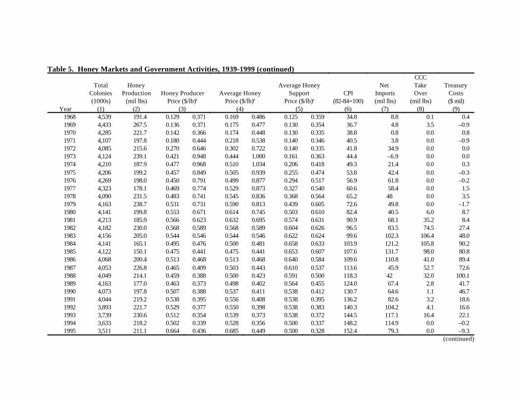
Table 5. Honey Markets and Government Activities, 1939-1999 (continued)

Year

TotalColonies(1000s)

(1)

HoneyProduction

(mil lbs)(2)

Honey ProducerPrice ($/lb)a

(3)

Average HoneyPrice ($/lb)a

(4)

Average HoneySupport

Price ($/lb)a

(5)

CPI(82-84=100)

(6)

Net Imports(mil lbs)

(7)

CCCTakeOver

(mil lbs)(8)

TreasuryCosts($ mil)

(9)1968 4,539 191.4 0.129 0.371 0.169 0.486 0.125 0.359 34.8 8.8 0.1 0.4 1969 4,433 267.5 0.136 0.371 0.175 0.477 0.130 0.354 36.7 4.8 3.5 –0.9 1970 4,285 221.7 0.142 0.366 0.174 0.448 0.130 0.335 38.8 0.8 0.0 0.8 1971 4,107 197.8 0.180 0.444 0.218 0.538 0.140 0.346 40.5 3.8 0.0 –0.9 1972 4,085 215.6 0.270 0.646 0.302 0.722 0.140 0.335 41.8 34.9 0.0 0.0 1973 4,124 239.1 0.421 0.948 0.444 1.000 0.161 0.363 44.4 –6.9 0.0 0.0 1974 4,210 187.9 0.477 0.968 0.510 1.034 0.206 0.418 49.3 21.4 0.0 0.3 1975 4,206 199.2 0.457 0.849 0.505 0.939 0.255 0.474 53.8 42.4 0.0 –0.3 1976 4,269 198.0 0.450 0.791 0.499 0.877 0.294 0.517 56.9 61.8 0.0 –0.2 1977 4,323 178.1 0.469 0.774 0.529 0.873 0.327 0.540 60.6 58.4 0.0 1.5 1978 4,090 231.5 0.483 0.741 0.545 0.836 0.368 0.564 65.2 48 0.0 3.5 1979 4,163 238.7 0.531 0.731 0.590 0.813 0.439 0.605 72.6 49.8 0.0 –1.7 1980 4,141 199.8 0.553 0.671 0.614 0.745 0.503 0.610 82.4 40.5 6.0 8.7 1981 4,213 185.9 0.566 0.623 0.632 0.695 0.574 0.631 90.9 68.1 35.2 8.4 1982 4,182 230.0 0.568 0.589 0.568 0.589 0.604 0.626 96.5 83.5 74.5 27.4 1983 4,156 205.0 0.544 0.546 0.544 0.546 0.622 0.624 99.6 102.3 106.4 48.0 1984 4,141 165.1 0.495 0.476 0.500 0.481 0.658 0.633 103.9 121.2 105.8 90.2 1985 4,122 150.1 0.475 0.441 0.475 0.441 0.653 0.607 107.6 131.7 98.0 80.8 1986 4,068 200.4 0.513 0.468 0.513 0.468 0.640 0.584 109.6 110.8 41.0 89.4 1987 4,053 226.8 0.465 0.409 0.503 0.443 0.610 0.537 113.6 45.9 52.7 72.6 1988 4,049 214.1 0.459 0.388 0.500 0.423 0.591 0.500 118.3 42 32.0 100.1 1989 4,163 177.0 0.463 0.373 0.498 0.402 0.564 0.455 124.0 67.4 2.8 41.7 1990 4,073 197.8 0.507 0.388 0.537 0.411 0.538 0.412 130.7 64.6 1.1 46.7 1991 4,044 219.2 0.538 0.395 0.556 0.408 0.538 0.395 136.2 82.6 3.2 18.6 1992 3,893 221.7 0.529 0.377 0.550 0.398 0.538 0.383 140.3 104.2 4.1 16.6 1993 3,739 230.6 0.512 0.354 0.539 0.373 0.538 0.372 144.5 117.1 16.4 22.1 1994 3,633 218.2 0.502 0.339 0.528 0.356 0.500 0.337 148.2 114.9 0.0 –0.2 1995 3,511 211.1 0.664 0.436 0.685 0.449 0.500 0.328 152.4 79.3 0.0 –9.3

(continued)

Table 5. Honey Markets and Government Activities, 1939-1999 (continued)

Year

TotalColonies(1000s)

(1)

HoneyProduction

(mil lbs)(2)

Honey ProducerPrice ($/lb)a

(3)

Average HoneyPrice ($/lb)a

(4)

Average HoneySupport

Price ($/lb)a

(5)

CPI(82-84=100)

(6)

Net Imports(mil lbs)

(7)

CCCTakeOver

(mil lbs)(8)

TreasuryCosts($ mil)

(9)1996 3,427 199.5 0.864 0.551 0.888 0.566 NAc NAc 156.9 140.7 0.0 –14.01997 3,494 196.5 0.722 0.450 0.752 0.469 NAc NAc 160.5 158.5 0.0 –1.51998 3,496 220.3 0.629 0.386 0.655 0.402 NAc NAc 163 122.0 0.0 0.01999 3,551 205.2 0.561 0.337 0.599 0.360 NAc NAc 166.6 161.0 0.0 2.4

a First price listed is the nominal price. Second price listed is the real price (1982-84=100).b Data not available.c Not applicable; no price supports during these years.

Sources:

Total Colonies: 1950-1987: Hoff and Phillips, 1990 (1988-1992: USDA, ERS Honey Background for 1995 Farm Legislation. 1993-1996: NASS, “Honey” annual issues 1995,1996, 1997). To account for changes in USDA data collection procedures, we added 863,000 to the official estimates from 1992 to 1999 (see appendix).

Honey Production: 1950-1991: Honey: Background for 1995 Farm Legislation by Frederic L. Hoff. 1992-1999: 2000 Agricultural Statistics(http://www.usda.gov/nass/pubs/agstats.htm).

Honey Producer Price (60 pound containers): 1939-1949: Estimates obtained using Average Honey Price (Producer Price = -.0504 + 1.0323·Average Honey Price, R2=.99. 1950-1959: ASCS Commodity Fact Sheet, June 1987. 1960-1986: ASCS Commodity Fact Sheet, October 1991. 1987-1999: NASS, "Honey,” annual issues.

Average Honey Price: 1939-1949: Agricultural Statistics, 1954, p. 90. 1950-1987: Hoff and Phillips, 1990. 1987-1991: NASS, “Honey,” annual issues. 1992-1999: 2000Agricultural Statistics (http://www.usda.gov/nass/pubs/agstats.htm). Average Honey Price is a weighted average of prices received by producers in wholesale and retail sales. Average Honey Price and Producer Price coincide 1982 to 1986 because data on retail sales were not collected.

Average Honey Support Price: 1950-1988: Hoff and Phillips, 1990. 1988-1995: USDA/ERS Sugar and Sweetener, Situation and Outlook Yearbook 1996. No support priceswere in effect after 1995.

CPI: Bureau of Labor Statistics Data (http://146.4.24/cgi-bin/surveymost).

Net Imports: 1950-1993: Honey: Background for 1995 Farm Legislation by Frederic L. Hoff. 1994-1999: Sugar: World Markets and Trade, USDA, FAS, annual issues(http://www.fas.usda.gov/htp2/sugar/1999/november/toc.html).

CCC Take Over: 1950-1984: Hoff and Phillips, 1990. 1985-1995: USDA Sugar and Sweetener, Situation and Outlook Yearbook 1996.

Treasury Costs: 1961-1984: Honey: Background for 1995 Farm Legislation by Frederic L. Hoff. Fiscal Year values. 1985-1995: Sugar and Sweetener, Situation and OutlookYearbook, December 1996. 1996-1999: History of Budgetary Expenditures of the Commodity Credit Corporation (http://www.fsa.usda.gov/dam/bud/indexccc.htm).

Table 6. U.S. Imports of Honey from China and Argentina, 1992-1999

1992 1993 1994 1995 1996 1997 1998 1999

China 60.0 76.6 64.5 27.5 42.7 25.2 26.9 47.9

Argentina 31.1 35.9 40.2 27.6 68.2 106.9 76.2 86.2

Total U.S.Imports

114.4 133.3 123.0 88.4 148.5 165.3 132.4 169.8a

aForecast

Source: USDA Agriculture Statistics and National Honey Board Statistics (http://www.nhb.org/intl/INTL_4Country1.gif and http://www.nhb.org/intl/SupplyProps2.gif).

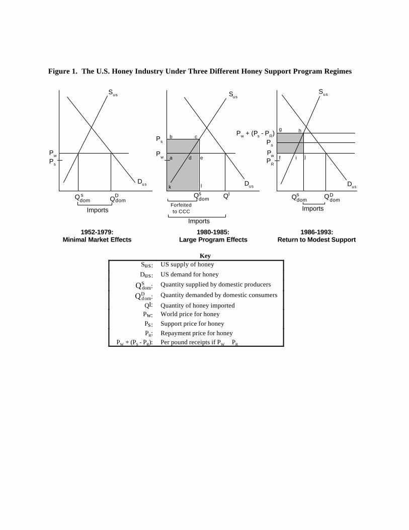
Sus

Pw

Ps

Dus

Pw + (Ps - PR)

Qsdom QD

dom

Imports

Qsdom QI

Forfeitedto CCC

Imports

dom Qdom

Imports

Q s D

1952-1979:Minimal Market Effects

1980-1985:Large Program Effects

1986-1993:Return to Modest Support

b

a

c

d e f i

l

g h

j

k

Sus

Pw

Ps

Dus

Sus

Dus

Pw

Ps

PR

Figure 1. The U.S. Honey Industry Under Three Different Honey Support Program Regimes

KeySus: US supply of honey

Dus: US demand for honey

QSdom: Quantity supplied by domestic producers

QDdom: Quantity demanded by domestic consumers

QI: Quantity of honey importedPw: World price for honeyPs: Support price for honeyPR: Repayment price for honey

PW + (PS - PR): Per pound receipts if PW Ö PR

1935 1940 1945 1950 1955 1960

Year

¢/lb

Producer Honey Price

Average Honey Price

Predicted Honey Price

0

5

10

15

20

25

30

Figure 2. Nominal Honey Prices, 1939-1959

(A2) y (

86 ' á (1%ã% ã2%ã3% ã4 ) % ã5 y(

81 % â (p86% ãp85% ã2 p84% ã3 p83% ã4 p82 )

% (å86% ãå85% ã2 å84% ã3å83% ã4å82) .

Appendix: Maximum Likelihood Estimation of the Colony Response Equation

We posit a partial adjustment model for the colony supply decision. This implies that the

current number of bee colonies is related to last year’s number of colonies and the current year’s ratio

of honey price to an index of production costs. The model is:

(A1) y (

t ' á % ã y(

t&1 % â p t % åt , t'51 ,... , 95,

where the åt are i.i.d. with Var(åt )= ó2. In (A1) denotes the true number of honeybee colonies andy(

t

pt denotes the price/cost ratio. The time index denotes year: “51” stands for “1951.”

Estimation of (A1) is complicated by the fact that colony numbers were not recorded for the

four years of 1982-1985. Prices and costs were recorded but there is no way to recover the

information on the dependent variable for the lost years. Further, because of the absence of , they(

85

observation for 1986 would need to be dropped in order to maintain the structure of a linear regression.

However, repeated back substitution of (A1) for the 1986 observation yields the following expression,

nonlinear in the parameters:

A second complication arises in trying to estimate the structural parameters from the observed

data. When the counting of honeybee colonies resumed in 1986, a change in data collection methods

yt(ã,A) ' yt & ãyt&1 , t ' 51, ..., 81

'yt & ã5 yt&1% A

(1% ã2% ã4

% ã6% ã8 )1/2

, t' 86

' yt & ãyt&1 % A(1& ã ) , t' 87,..., 95 ,

resulted in (at least) a level change in the number of colonies counted. It is reported in USDA

publications that small beekeepers were not surveyed under the new scheme. We model this change in

survey techniques as a fixed constant, A, by which post-1981 colony estimates understate the true

number of colonies:

(A3) yt ' y(

t & A, t' 82, ..., 95 ,

where yt denotes the recorded colony count. Prior to 1982, we assume that .yt ' y (

t

Substituting from (A3) into (A2) gives the following nonlinear regression model:

(A4) y t(ã, A) ' á d t(ã) % â p t(ã) % ut , t' 51, ...,81,86, ..., 95 ,

where

d t(ã) ' 1 , t Ö 86 ,

'1% ã% ã2% ã3% ã4

(1% ã2% ã4

% ã6% ã8 )1/2

, t ' 86 .

p t(ã) ' pt , t Ö 86 ,

'p86% ãp85% ã2 p84% ã3 p83% ã4 p82

(1% ã2% ã4

% ã6% ã8 )1/2

, t' 86 .

ln L(ã, A, á , â) ' &T2

ln(2ð%1) & lnó2 (ã, A, á , â) ,

The disturbance is i.i.d. with Var(ut) = ó2.

If the ut are assumed to be normally distributed, and if the nuisance parameter, ó2, is

concentrated out, the log-likelihood function for the model is:

where ó2 (ã, A, á, â) '1T j ( yt& á d t& âp t )2 .

The last expression shows that maximum likelihood is equivalent to nonlinear least squares. The ML

estimate of the colony response equation is shown in table 1.