PROGRAM ON THE GLOBAL DEMOGRAPHY OF AGING

Working Paper Series

The Fertility Transition Around the World -1950-2005

Holger Strulik and Sebastian Vollmer

March 2010

PGDA Working Paper No. 57 http://www.hsph.harvard.edu/pgda/working.htm

The views expressed in this paper are those of the author(s) and not necessarily those of the Harvard Initiative for Global Health. The Program on the Global Demography of Aging receives funding from the National Institute on Aging, Grant No. 1 P30 AG024409-06.

The Fertility Transition Around the World – 1950-2005

Holger Strulik∗ and Sebastian Vollmer∗∗

March 2010

Abstract. In this paper we analyze the distribution of fertility rates across the

world using parametric mixture models. We demonstrate the existence of twin

peaks and the division of the world’s countries in two distinct components: a

high-fertility regime and a low fertility regime. Whereas the significance of

twin peaks vanishes over time, the two fertility regimes continue to exists

over the whole observation period. In 1950 about two thirds of the world’s

countries belonged to the high-fertility regime and the rest constituted the

low-fertility regime. By the year 2005 this picture has reversed. Within both

the low- and the high-fertility regime the average fertility rate declined, with

a larger absolute decline within the high-fertility regime. Visually, the two

peaks moved closer together. For the low fertility-group we find both β- and

σ- convergence but we cannot establish any convergence pattern for the high

fertility regime. Overall our findings are difficult to reconcile with the standard

view of a fertility trap but they support the “differentiated take-off” view

established in the Unified Growth literature.

Keywords: Fertility, Convergence, Twin Peaks, Fertility Regimes, Unified

Growth.

∗Department of Economics, Brown University, Providence, RI 02912, USA, email: holger strulik@brown.eduand University of Hannover, Wirtschaftswissenschaftliche Fakultaet, 30167 Hannover, Germany; email:strulik@vwl.uni-hannover.de.∗∗Harvard University, Center for Population and Development Studies, 9 Bow Street, Cambridge, MA 02138;email: svollmver@hsph.harvard.edu.

1. Introduction

Over the last two hundred years of human history every successfully developing country

experienced a fertility transition: starting at initially high levels, fertility rates went down

towards a low plateau, sometimes below replacement level. This one-time demographic event

seems to be so inevitably linked with economic growth that many researchers are starting to

understand the fertility transition as a prerequisite for successful development (see Galor, 2005,

for an overview). In almost all cases the fertility transition was lead by a secular fall of mortality

rates so that it seems that decreasing mortality rates have caused fertility to fall. However, there

are certainly other forces at work as well since the specific pattern of the fertility transition differs

substantially across countries (see e.g. Chesnais, 1992, Lee, 2003, Reher, 2003).

The Western European countries and their Western offshoots (the U.S., Canada) experienced

the transition first around the end of the nineteenth century. One salient feature of their transi-

tion was the chronological proximity between the onsets of mortality decline and fertility decline

(0-10 years). This chronological association became much less visible for countries which ex-

perienced the fertility transition later. If the fertility decline took off in the 1980s or later it

followed the mortality decline with an average delay of 40-45 years (Reher, 2003). Until today,

some countries, notably from Sub-Saharan Africa, show so little tendency for declining fertility

that the question arises whether the fertility transition is indeed a world-wide phenomenon or

whether there exists a “fertility trap” that hinders some countries to follow the path of the

historical leaders.1

In the economics literature the catch up process is statistically assessed with tests for so

called β- and σ-convergence. These tools have been developed in the context of the take off

towards long-run income growth (Barro and Sala-i-Martin, 1992). But they are easily adapted to

analyze the fertility transition. Here, β-convergence applies if countries of initially high fertility

experience a stronger decline of fertility than countries of initially low fertility. σ-convergence

occurs if the cross-sectional dispersion, measured by the standard deviation of fertility, for a

group of countries declines over time. These concepts are not redundant. While β convergence

implies a tendency for σ convergence, it is not sufficient because countries are also affected by

1The notion of a fertility trap originates from Malthus (1798). Nelson (1956) is a first modern formulation of theidea as a locally stable equilibrium. See also, among others, Koegel and Prskawetz (2001) and Strulik (2004). Witha different notion of glacier-slow development (rather than local stability) the Malthusian trap is also discussedin the unified growth literature, see Galor (2005).

1

fertility unrelated shocks. In turn, the observation of decreasing dispersion does not necessarily

entail β-convergence. In the economics literature it is also an ongoing debate whether the

world income distribution is twin-peaked and wether there is “club convergence”, i.e. converging

income levels within specific groups of countries but diverging income levels between the these

groups or “convergence clubs”.2

Recently a couple of articles addressed the problem of converging or non-converging vital

rates across the world. Using histograms and inference from eyeballing, Wilson (2001) found

twin peaks of the distribution of world-wide population weighted fertility in the 1950s, which

vanished over time until the year 2000. From that he concluded that “we are moving into a

world where the distinction between developed and developing countries is of greatly diminished

relevance to fertility” and that “the overwhelming trend is for low fertility to become a general

feature of poor and rich countries”. Using the β- and σ-convergence criterion, Dorius (2008)

arrived at a much less optimistic conclusion by observing that countries began only recently

to converge towards less differentiated fertility rates. Using a set of inequality measures he

actually finds evidence for diverging fertility rates over the last half century. In a related study

on mortality, Bloom and Canning (2007) find evidence for a twin-peaked distribution and a

“mortality trap”. Using a mixture model they are able to identify a high mortality and a

low mortality regime and estimate the probability of being in the low-mortality regime to be

positively related to initial life-expectancy in 1963.

Here we take up from Bloom and Canning (2007) the idea of the world being divided in

different regimes and apply it to the fertility transition. Using a parametric mixture model

we are able to scrutinize these earlier convergence results. The method is particularly useful

since it does not a priori assign the world’s countries into different groups by imposing a certain

threshold, nor does it impose a particular assumption on the number of ”convergence clubs”.

Our results provide a rejoinder of the previous conflicting views on the fertility transition and

some interesting further results. Using modern econometric methods we confirm that the world’s

fertility distribution became indeed single-peaked after 1990. At the same time, however, we also

firmly established that from the beginning of our observation period in 1950 until the end in 2005

2The twin peak debate originated from Quah (1993, 1996), see also Jones (1997), Kremer et al. (2001), andFeyrer (2008). For a comprehensive introduction of β and σ-convergence see Chapter 11 of Barro and Sala-i-Martin (2004), for a broader discussion of convergence and convergence clubs see also Baumol (1986), Durlaufand Johnson (1995), Azariades (1996), Galor (1996), Pritchett (1997), and Pomeranz (2000). For the debate on alow level equilibrium or poverty trap see, among many others, Bloom and Canning (2003), Graham and Temple(2006), and Kray and Radatz (2007).

2

there exist two distinct components of the world fertility distribution: a high-fertility regime

and a low-fertility regime. Within both regimes fertility is falling over time albeit starting from

a much higher initial level in the high fertility regime. We also observe σ-convergence across the

world and within the low fertility regime but not within the high-fertility regime. Furthermore

we show β-convergence within the low-fertility regime but not within the high fertility regime.

These findings suggest the following assessment of the world fertility transition. For countries

within the low fertility regime there exists a strong tendency to converge towards a common

low fertility rate below replacement level. Initial fertility is a good predictor for future fertility

decline. The high-fertility regime, on the other hand, is not a convergence club and, consequently,

it is difficult to conceptualize the countries belonging to this regime as being stuck in a “high-

fertility” trap or, more formally, approaching a locally stable high-fertility-equilibrium. This

view is substantiated by the fact that most countries in the high-fertility group also experience

some decrease of fertility over time and, more importantly, by the fact that between 1950 and

2005 altogether 49 high-fertility countries were able to enter the low-fertility regime. Moreover,

initial fertility is not a good predictor for leaving the high-fertility group.

This assessment of the world fertility transition supports recent insights from unified growth

theory (see Galor 2005, 2009 for overviews). Using dynamic general equilibrium models with

demographic-economic feedback effects this literature argues that the view of the world as being

divided into clubs of countries diverging toward different locally stable equilibria, with initial

conditions (initial fertility rates) determining the direction of development, is misleading. In-

stead, unified growth theory suggests that all countries evolved from an epoch of quasi-stagnation

and high fertility towards high growth and low fertility and that geographic and biological fun-

damentals determine the timing of the take off towards high growth and low fertility.3

In other words, unified growth theory conceptualizes the world as divided in different regimes,

within one regime the take off is not yet visible, within the other regime we see convergence.

Potentially there could be a third regime consisting of countries on the way from the high-

fertility regime towards the low-fertility regime. Given that the movement between low and

high-fertility regime is sufficiently fast and/or that at each time interval there are sufficiently

few countries “on the move”, the movers are not discernable as a separate group, and there

3The unified growth view originates from Galor and Weil (2000). The differentiated take-off view was popularizedby Lucas (2000). See Strulik (2008a,b) for a theoretical approach on the geographical distribution of the onset offertility transition.

3

are just two regimes. In contrast to the fertility trap view, however, a country’s association

with the not-yet-converging regime is potentially temporary. A country’s initial fertility rate

is not a good predictor of the take-off because the differentiated take-off over time originates

from fundamentals rather than initial values. Only for countries which successfully entered the

low-fertility regime the theory predicts convergence as fertility rates during the initiated fertility

transition approach a low-level. This is exactly what we find confirmed in the data.

2. Data and Method

In the economics literature the notion of twin peaks in the cross-country income distribution

was introduced by Quah (1996). He interpreted the emergence of twin peaks as polarization of

the cross-country income distribution into a rich and a poor convergence club. Diagrammatically,

twin peaks can be observed by non-parametric kernel density estimation. But this method leaves

open the question of their econometric significance. For that purpose, Silverman (1981) showed

that the number of peaks of a kernel density estimator is a right-continuous, monotonically

decreasing function of the bandwidth for normal kernels. This allowed him to define the k-

critical bandwidth as the minimal bandwidth such that the density still has k peaks and not

yet k + 1 peaks. Based on the notion of the k-critical bandwidth, Silverman (1981) proposed a

bootstrap test for the hypothesis of k peaks against the alternative of more than k peaks. Bianchi

(1997) was the first to apply Silverman’s test to cross-country income data and he confirmed

Quah’s hypothesis.

More recently, Holzmann et al. (2007) pointed out that it is misleading to look at the number

of peaks of the cross-country income distribution. They show that simple rescaling of the

data (e.g. taking logs) produces a statistically significant triple peaked cross-country income

distribution. Countries which were previously assigned to Quah’s poor convergence club are

now considered middle-income on the log-scale, which obviously doesn’t make much sense for

economic interpretation. Holzmann et al. (2007) propose an alternative methodology which

is invariant to strictly monotonic transformation of the data and is thus robust towards this

shortcoming of the twin peaks approach. We are going to adopt their approach for the cross-

country distribution of fertility rates.

We use the United Nations World Population Prospects (2008 Revision) to obtain data on

the total fertility rate of 184 countries over the period of 1950 to 2005. The data comes in

4

eleven intervals of five year length and includes no missing values. Exploratory data analysis

with kernel density estimators reveals a twin peak phenomenon similar to income data and thus

requires similar techniques to model it.

Following Holzmann et al. (2007) and Vollmer et al. (2009) we model the cross-country

distribution of fertility rates as a finite mixture. In a two-component normal mixture, the

observations have density

f(x;α, µ1, µ2, σ1, σ2) = (1− α)φ(x;µ1, σ1) + αφ(x;µ2, σ2), (1)

with 0 ≤ α ≤ 1 and

φ(x;µ, σ) =1√

2πσ2exp

(−(x− µ)2

2σ2

).

We assume without loss of generality that µ1 ≤ µ2. φ(x;µ1, σ1) and φ(x;µ2, σ2) correspond to

the distributions of the two assumed sub-populations, and α and 1− α are interpreted as their

relative sizes.

Note that it is essential to set up a joint model for the two sub-populations, since we want

to investigate convergence within the complete distribution. The parameters α, µ1, µ2, σ1 and

σ2 are estimated from the data by the method of maximum likelihood. We allow for unequal

variances σ21 and σ22, because a likelihood ratio test shows that the simplifying assumption of

equal variances does not hold for all years.

One of our most important results that we establish below is that a mixture of two one-peaked

distributions can have one or two peaks. This is so because two distributions will overlap if

they are sufficiently close together such that the peaks of the two underlying distributions will

merge into one. Our methodology thus has the additional advantage that it can still identify

heterogeneity in cases where multiple peaks are not visible and/or a statistical test for their

significance fails. Moreover, we can calculate for each observation the posterior probabilities

p1 and p2 for belonging to the first or respectively second component of the mixture model.

This allows us to assign each observation to one of the components depending on which of the

two probabilities is higher. Movements between the components are of particular interest, this

essentially means that we observe p1 < p2 in one year and p2 > p1 in another year.

The likelihood function in finite normal mixtures with different variances is unbounded, thus,

a global maximizer of the likelihood function does not exist. However, when using reasonable

5

starting values maximization algorithms such as EM or quasi Newton find stable local maxima

of the log-likelihood function.

To substantiate our findings it is, of course, essential that we formally validate that there are

indeed two components necessary to model the data, i.e. that we test the hypothesis that there

are two components against the alternative that a single component is sufficient to describe the

world fertility distribution accurately. This turns out to be a quite difficult parametric testing

problem; see Chen and Chen (2003) for some history of attempts to solve it. Here, we will use

a novel approach, the EM-test developed by Chen and Li (2008) for normal mixtures in mean

and variance parameters, a test which overcomes many drawbacks of the simple likelihood ratio

test for the same problem. It was first introduced to the economic literature by Vollmer et al.

(2009). Details on the methodology are provided by Chen and Li (2008) and Vollmer et al.

(2009).

3. Results

We begin with testing for the number of components and the number of peaks of the world

fertility distribution. The test for the number of components finds that the hypothesis of just

one component can be rejected with a p-value smaller than 0.01 in all subperiods from 1950

to 2005. The test for the number of peaks is reported in Table 1. Over the whole observation

period the hypothesis of two peaks cannot be rejected in favor of more than two peaks. Thus

there are at most two peaks. Until 1990 we can firmly reject the hypothesis that there is just one

peak. Afterwards the second peak vanishes over time. In subperiod 1990-1995 the second peak

is still weakly significant at a 10 percent level, for the two latest intervals it becomes statistically

insignificant.

These observations reconcile the seemingly conflicting views on fertility convergence sketched

in the Introduction. A vanishing twin peak is compatible with the view of a world divided

into two different fertility regimes, one formed by the high-fertility component, the other by the

low-fertility component.

Using the results reported in Table 2 we can explain how the two-component distribution

morphed from twin-peaked towards single-peaked. Both component-means declined gradually

over time. While the mean of the high-fertility component declined from 6.47 to 4.39, the

mean of the low fertility component declined from an already low initial mean of 3.14 to 1.89

6

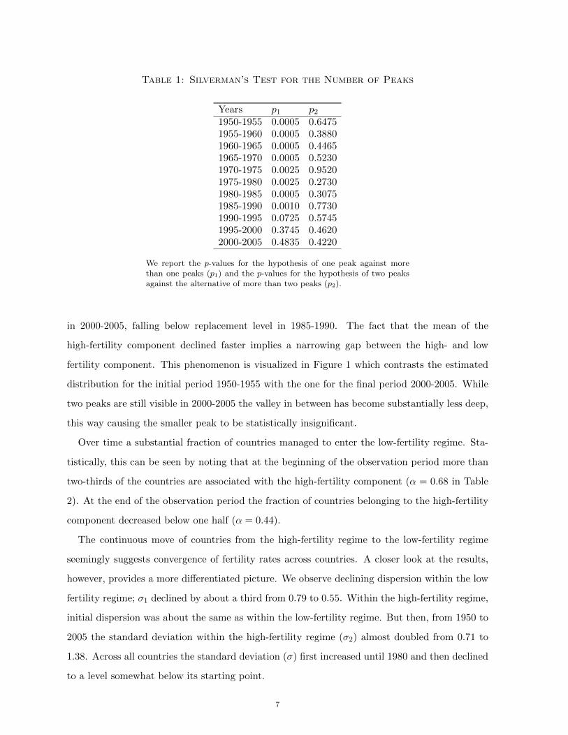
Table 1: Silverman’s Test for the Number of Peaks

Years p1 p21950-1955 0.0005 0.64751955-1960 0.0005 0.38801960-1965 0.0005 0.44651965-1970 0.0005 0.52301970-1975 0.0025 0.95201975-1980 0.0025 0.27301980-1985 0.0005 0.30751985-1990 0.0010 0.77301990-1995 0.0725 0.57451995-2000 0.3745 0.46202000-2005 0.4835 0.4220

We report the p-values for the hypothesis of one peak against morethan one peaks (p1) and the p-values for the hypothesis of two peaksagainst the alternative of more than two peaks (p2).

in 2000-2005, falling below replacement level in 1985-1990. The fact that the mean of the

high-fertility component declined faster implies a narrowing gap between the high- and low

fertility component. This phenomenon is visualized in Figure 1 which contrasts the estimated

distribution for the initial period 1950-1955 with the one for the final period 2000-2005. While

two peaks are still visible in 2000-2005 the valley in between has become substantially less deep,

this way causing the smaller peak to be statistically insignificant.

Over time a substantial fraction of countries managed to enter the low-fertility regime. Sta-

tistically, this can be seen by noting that at the beginning of the observation period more than

two-thirds of the countries are associated with the high-fertility component (α = 0.68 in Table

2). At the end of the observation period the fraction of countries belonging to the high-fertility

component decreased below one half (α = 0.44).

The continuous move of countries from the high-fertility regime to the low-fertility regime

seemingly suggests convergence of fertility rates across countries. A closer look at the results,

however, provides a more differentiated picture. We observe declining dispersion within the low

fertility regime; σ1 declined by about a third from 0.79 to 0.55. Within the high-fertility regime,

initial dispersion was about the same as within the low-fertility regime. But then, from 1950 to

2005 the standard deviation within the high-fertility regime (σ2) almost doubled from 0.71 to

1.38. Across all countries the standard deviation (σ) first increased until 1980 and then declined

to a level somewhat below its starting point.

7

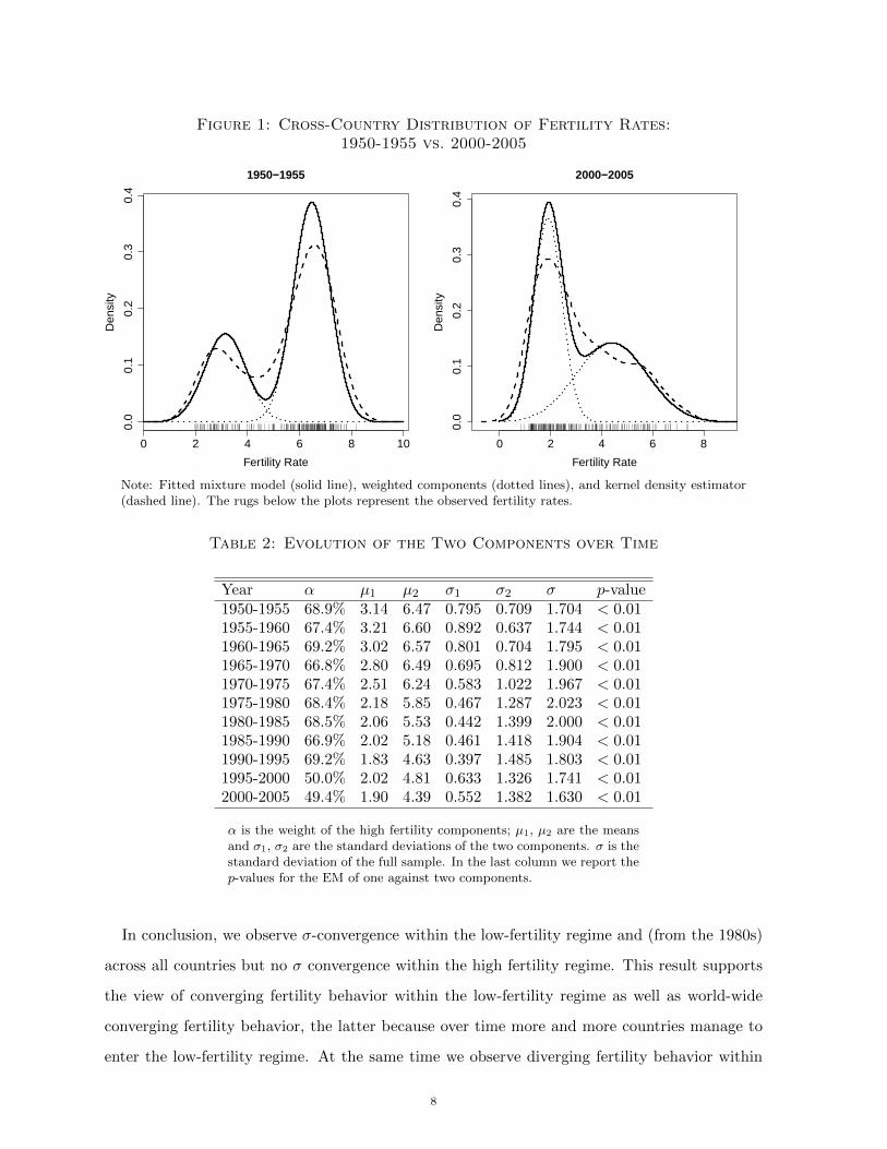
Figure 1: Cross-Country Distribution of Fertility Rates:1950-1955 vs. 2000-2005

0 2 4 6 8 10

0.0

0.1

0.2

0.3

0.4

1950−1955

Fertility Rate

Den

sity

0 2 4 6 80.

00.

10.

20.

30.

4

2000−2005

Fertility Rate

Den

sity

Note: Fitted mixture model (solid line), weighted components (dotted lines), and kernel density estimator(dashed line). The rugs below the plots represent the observed fertility rates.

Table 2: Evolution of the Two Components over Time

Year α µ1 µ2 σ1 σ2 σ p-value1950-1955 68.9% 3.14 6.47 0.795 0.709 1.704 < 0.011955-1960 67.4% 3.21 6.60 0.892 0.637 1.744 < 0.011960-1965 69.2% 3.02 6.57 0.801 0.704 1.795 < 0.011965-1970 66.8% 2.80 6.49 0.695 0.812 1.900 < 0.011970-1975 67.4% 2.51 6.24 0.583 1.022 1.967 < 0.011975-1980 68.4% 2.18 5.85 0.467 1.287 2.023 < 0.011980-1985 68.5% 2.06 5.53 0.442 1.399 2.000 < 0.011985-1990 66.9% 2.02 5.18 0.461 1.418 1.904 < 0.011990-1995 69.2% 1.83 4.63 0.397 1.485 1.803 < 0.011995-2000 50.0% 2.02 4.81 0.633 1.326 1.741 < 0.012000-2005 49.4% 1.90 4.39 0.552 1.382 1.630 < 0.01

α is the weight of the high fertility components; µ1, µ2 are the meansand σ1, σ2 are the standard deviations of the two components. σ is thestandard deviation of the full sample. In the last column we report thep-values for the EM of one against two components.

In conclusion, we observe σ-convergence within the low-fertility regime and (from the 1980s)

across all countries but no σ convergence within the high fertility regime. This result supports

the view of converging fertility behavior within the low-fertility regime as well as world-wide

converging fertility behavior, the latter because over time more and more countries manage to

enter the low-fertility regime. At the same time we observe diverging fertility behavior within

8

the high-fertility regime, a first indication that the high- fertility regime may be difficult to

interpret as a locally stable development trap.

The results for 1950-1955 and 2000-2005 are visualized in Figure 1 (c.f. Figure 4 in the

appendix for all other years). In 1950-1955 the peaks were equally wide, but the peak of the

high fertility regime is much higher than the peak of the low fertility regime because about

two thirds of the countries are assigned to the high fertility regime. The overlap of the two

distributions is very small. In 2000-2005 the two distributions have approximately the same

area (α ≈ 0.5). But the peak of the low fertility regime is tall and slim whereas the peak of

the high fertility regime is short and wide. The overlap between the two distributions is now

substantial. This explains why the second peak is not significant anymore (Table 1) although

still discernable in Figure 1.

Figure 2: Cross-Country Distribution of Fertility Rates: 1950-1955 vs.2000-2005

2 3 4 5 6 7 8

−5

−4

−3

−2

−1

0

Fertility in 1950−1955

Fer

tility

Cha

nge

1950−

2005

5.0 5.5 6.0 6.5 7.0 7.5 8.0

−5

−4

−3

−2

−1

0

High Fertility Regime

Fertility in 1950−1955

Fer

tility

Cha

nge

1950

−20

05

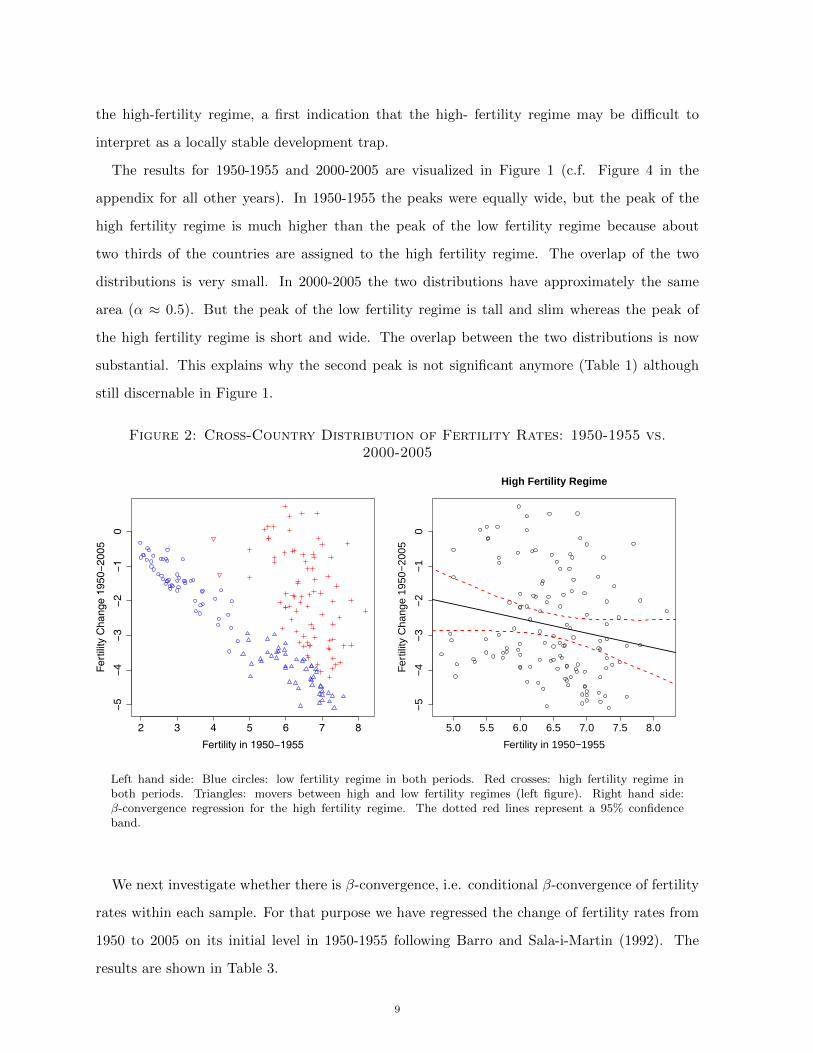
Left hand side: Blue circles: low fertility regime in both periods. Red crosses: high fertility regime inboth periods. Triangles: movers between high and low fertility regimes (left figure). Right hand side:β-convergence regression for the high fertility regime. The dotted red lines represent a 95% confidenceband.

We next investigate whether there is β-convergence, i.e. conditional β-convergence of fertility

rates within each sample. For that purpose we have regressed the change of fertility rates from

1950 to 2005 on its initial level in 1950-1955 following Barro and Sala-i-Martin (1992). The

results are shown in Table 3.

9

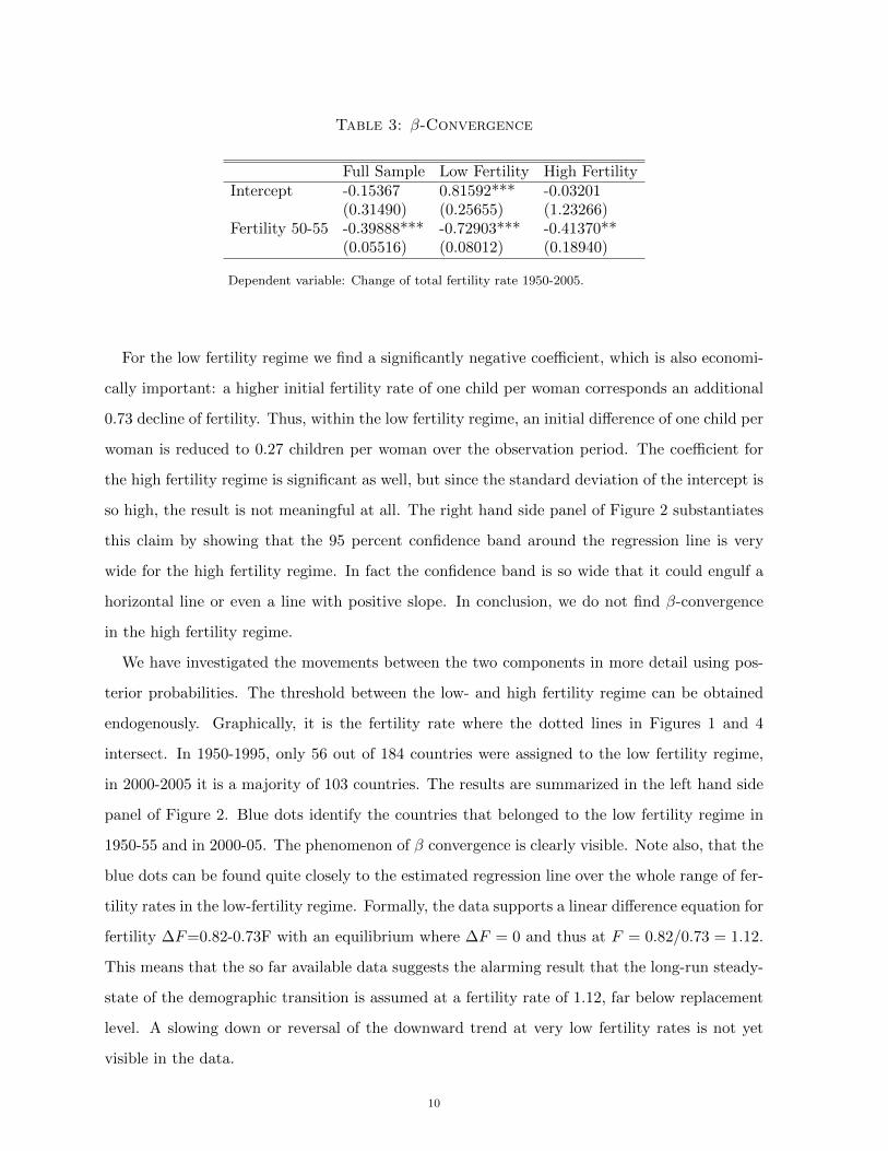
Table 3: β-Convergence

Full Sample Low Fertility High FertilityIntercept -0.15367 0.81592*** -0.03201

(0.31490) (0.25655) (1.23266)Fertility 50-55 -0.39888*** -0.72903*** -0.41370**

(0.05516) (0.08012) (0.18940)

Dependent variable: Change of total fertility rate 1950-2005.

For the low fertility regime we find a significantly negative coefficient, which is also economi-

cally important: a higher initial fertility rate of one child per woman corresponds an additional

0.73 decline of fertility. Thus, within the low fertility regime, an initial difference of one child per

woman is reduced to 0.27 children per woman over the observation period. The coefficient for

the high fertility regime is significant as well, but since the standard deviation of the intercept is

so high, the result is not meaningful at all. The right hand side panel of Figure 2 substantiates

this claim by showing that the 95 percent confidence band around the regression line is very

wide for the high fertility regime. In fact the confidence band is so wide that it could engulf a

horizontal line or even a line with positive slope. In conclusion, we do not find β-convergence

in the high fertility regime.

We have investigated the movements between the two components in more detail using pos-

terior probabilities. The threshold between the low- and high fertility regime can be obtained

endogenously. Graphically, it is the fertility rate where the dotted lines in Figures 1 and 4

intersect. In 1950-1995, only 56 out of 184 countries were assigned to the low fertility regime,

in 2000-2005 it is a majority of 103 countries. The results are summarized in the left hand side

panel of Figure 2. Blue dots identify the countries that belonged to the low fertility regime in

1950-55 and in 2000-05. The phenomenon of β convergence is clearly visible. Note also, that the

blue dots can be found quite closely to the estimated regression line over the whole range of fer-

tility rates in the low-fertility regime. Formally, the data supports a linear difference equation for

fertility ∆F=0.82-0.73F with an equilibrium where ∆F = 0 and thus at F = 0.82/0.73 = 1.12.

This means that the so far available data suggests the alarming result that the long-run steady-

state of the demographic transition is assumed at a fertility rate of 1.12, far below replacement

level. A slowing down or reversal of the downward trend at very low fertility rates is not yet

visible in the data.

10

Blue triangles in the left hand side panel of Figure 2 indicate countries that managed to

enter the low-fertility regime between 1950 and 2005. Interestingly, a number of countries with

very high initial fertility rates of more than seven managed to move into the low fertility regime

whereas some other countries with relatively low fertility rates (compared to the mean within the

high-fertility regime), i.e. countries with initial fertility rates around five, remained in the high-

fertility regime. This lets us conclude that the initial level of fertility is only a good predictor

for changes of fertility once the transition towards the low fertility regime has been made. The

take off towards the low fertility regime appears to be not predicted by the initial fertility rate.

Other, more fundamental forces are at work to determine the chronologically differentiated take

off across countries.

In Figure 3 we identify on a world map the countries which stayed in their initial regime

and the countries which managed to enter the low-fertility regime. In 1950-1955 most of Latin

America (except Argentina), Africa and Asia belonged to the high fertility regime. By 2000-

2005 most of Latin America and East Asia have transitioned into the low fertility regime, Africa

(except Morocco, Tunesia, Algeria, and South Africa), the Indian subcontinent and the Arabian

peninsula remained in the high fertility regime.

4. Conclusion

In this article we have investigated the evolution of the world fertility distribution and scruti-

nized the important question whether there is convergence of fertility behavior. For that purpose

we utilized a recently developed econometric machinery. Our most important findings are that

the world was and still is separated into a low-fertility regime and a high-fertility regime and

that this finding is consistent with the observation of a vanishing twin-peak. For the low fertility

regime we have demonstrated β- and σ-convergence, indicating an ongoing fertility transition

and that the countries belonging to this regime are indeed converging towards a common low

fertility rate below replacement level.

Within the high-fertility group we find neither β convergence nor σ-convergence. Actually,

countries belonging to this group seem to drift farther apart. Thus we find no evidence for a

“fertility trap” conceptualized as a locally stable equilibrium of underdevelopment. Again, the

notion of an absent fertility trap is consistent with the view of a world separated in different

11

fertility regimes. It supports the theoretical literature established by unified growth theory,

which argues in favor of a differentiated take off over time (rather than multiple equilibria).

Initial fertility rates are not a good predictor for the successful move towards the low fertility

regime. Yet quite a few countries managed this transition over last half century. This raises, of

course, the question, which are good predictors for the take off towards the low fertility regime.

We leave this question for future research. From inspection of the maps in Figure 3, geographic

location seems to be a good predictor, a conclusion that would be consistent with the theory of

a geographically differentiated take-off developed in Strulik (2008a,b).

An alarming finding is that our convergence results suggest that the fertility transition within

the low fertility regime is still ongoing at unchanged speed, with a predicted equilibrium at 1.12,

far below replacement level. Perhaps this assessment is too pessimistic and actual adjustment is

non-linear, with undershooting behavior and adjustment towards replacement level from below.

This view is theoretically supported by Strulik and Weisdorf (2008).

12

References

Azariadis, C., 1996, The economics of poverty traps, part one: Complete markets, Journal of

Economic Growth 1, 449-496.

Baumol, W., 1986, Productivity growth, convergence, and welfare, American Economic Review

76, 1072-1085.

Barro, R.J. and X. Sala-i-Martin, Economic Growth, 2nd ed., MIT Press, Cambridge, MA.

Bianchi, M., 1997, Testing for Convergence: Evidence from Non-Parametric Multimodality

Tests. Journal of Applied Econometrics 12, 393-409.

Bloom, D.E., D. Canning, and J. Sevilla, 2003, Geography and poverty traps, Journal of Eco-

nomic Growth 8, 355-378.

Bloom, D.E. and Canning, D., 2007, Mortality traps and the dynamics of health transitions,

Proceedings of the National Academy of Sciences 104, 16044-16049.

Chen, H. and J. Chen, 2003, Tests for homogeneity in normal mixtures with presence of a

structural parameter, Statistica Sinica 13, 351-365.

Chen, J. and P. Li, 2008, Hypothesis test for Normal Mixture Models: the EM Approach, Annals

of Statistics 37, 2523-2542.

Chesnais, J.-C., 1992, The Demographic Transition: Stages, Patterns, and Economic Implica-

tions, Oxford: Clarendon Press.

Dorius, S.F., 2008, Global convergence? A reconsideration of changing intercountry inequality

in fertility, Population and Development Review 34, 519-537.

Durlauf, S.N. and P. A. Johnson, 1995, Multiple Regimes and Cross-Country Growth Behavior,

Journal of Applied Econometrics 10, 365-384.

Galor, O., 1996, Convergence? Inferences from theoretical models, Economic Journal, 1056-

1069.

Galor, O. and D.N. Weil, 2000, Population, Technology, and Growth: From Malthusian Stagna-

tion to the Demographic Transition and Beyond, American Economic Review 90, pp. 806-828.

13

Galor, O., 2005, From stagnation to growth: unified growth theory, in: Handbook of Economic

Growth, Amsterdam: North-Holland.

Galor, O., 2009, Comparative economic development: insights from unified growth theory, 2008

Lawrence Klein Lecture, Discussion Paper, Brown University.

Graham, B.S. and J.R.W. Temple, 2006, Rich nations, poor nations: how much can multiple

equilibria explain?, Journal of Economic Growth 11, 5-41.

Holzmann, H., S. Vollmer and J. Weisbrod, 2007, Twin Peaks or Three Components? Discussion

Paper. University of Gottingen. Revised December 2009.

Jones, C.I., 1997, On the evolution of the world income distribution, Journal of Economic

Perspectives, 19-36.

Kogel, T., and A. Prskawetz, 2001, Agricultural productivity growth and escape from the

Malthusian trap, Journal of Economic Growth 6, 337-357.

Kraay, A., and C. Raddatz, 2007, Poverty traps, aid, and growth, Journal of Development

Economics 82, 315-347.

Kremer, M., A. Onatski, and J. Stock, 2001, Searching for prosperity, Carnagie-Rochester Con-

ference Series on Public Policy 55, 275-303.

Lee, R., 2003, The Demographic Transition: Three Centuries of Fundamental Change, Journal

of Economic Perspectives 17, 167-190.

Lucas, R.E. Jr., 2000, Some macroeconomics for the 21st century, Journal of Economic Per-

spectives 11(4), 159-168

Malthus, T.R., 1798, An Essay on the Principle of Population.

Nelson, R., 1956, A theory of the low-level equilibrium trap in under-developed economies,

American Economic Review 46, 894-908.

Pomeranz, K., 2000, The Great Divergence: China, Europe, and the Making of the Modern

World Economy, Princeton University Press, Princeton.

Pritchett, L., 1997, Divergence, big time, Journal of Economic Perspectives

14

Quah, D.T., 1993, Galton’s fallacy and tests of the convergence hypothesis, Scandinavian Journal

of Economics 95, 427-443.

Quah, D.T., 1996, Empirics for economic growth and convergence, European Economic Review

40, 1353-1375.

Reher, D.S., 2004, The Demographic transition revisited as a global process, Population, Space

and Place 10, 19-41.

Silverman, B., 1981, Using kernel density estimates to investigate multimodality, Journal of the

Royal Statistical Society Series B 43, 97-99.

Strulik, H., 2004, Economic growth and stagnation with endogenous health and fertility, Journal

of Population Economics 17, 433-453.

Strulik, H., 2008a, Geography, health, and the pace of demo-economic develoment, Journal of

Development Economics 86, 61-75.

Strulik, H., 2008b, Degrees of develoment, Discussion Paper, University of Hannover.

Strulik, H. and Weisdorf, J., 2008, Population, Food, and Knowledge: A Simple Unified Growth

Theory, Journal of Economic Growth 13, 169-194.

United Nations, Department of Economic and Social Affairs, Population Division, World Pop-

ulation Prospects: The 2008 Revision, New York, 2009, http://data.un.org/.

Vollmer, S., H. Holzmann, F. Ketterer and S. Klasen, 2009, Diverging Convergence in Unified

Germany, Discussion Paper, University of Hannover.

Wilson, C., 2001, On the scale of global demographic convergence 1950-2000, Population and

Development Review 27, 155-171.

15

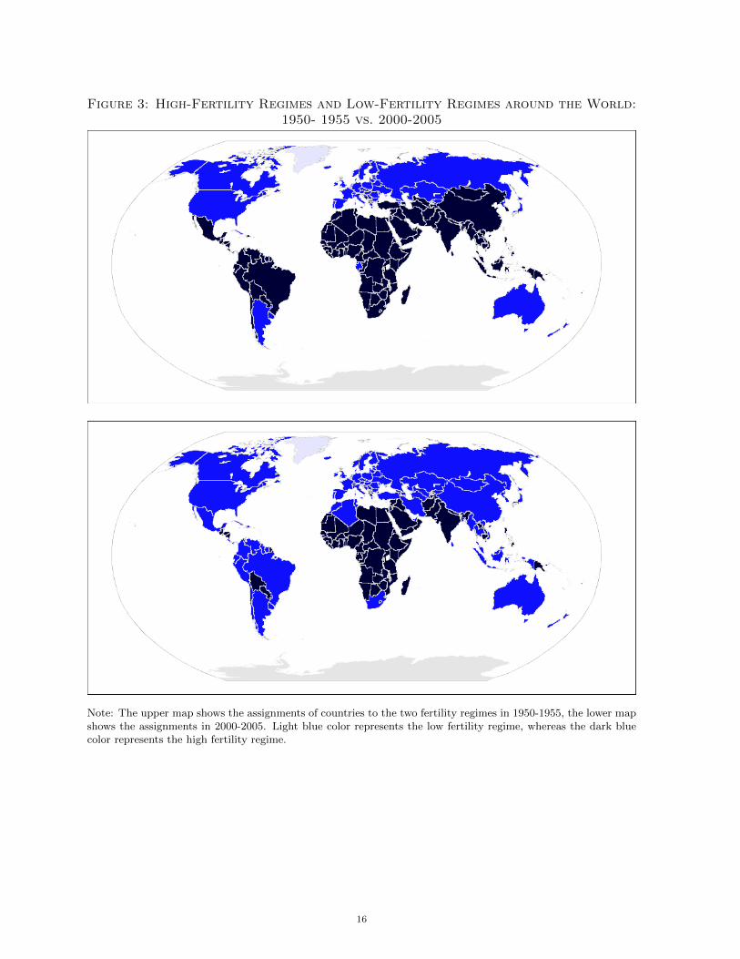
Figure 3: High-Fertility Regimes and Low-Fertility Regimes around the World:1950- 1955 vs. 2000-2005

Note: The upper map shows the assignments of countries to the two fertility regimes in 1950-1955, the lower mapshows the assignments in 2000-2005. Light blue color represents the low fertility regime, whereas the dark bluecolor represents the high fertility regime.

16

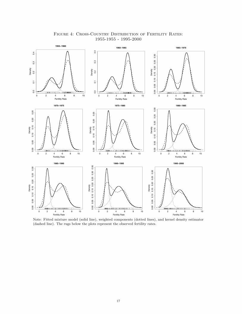
Figure 4: Cross-Country Distribution of Fertility Rates:1955-1955 - 1995-2000

0 2 4 6 8 10

0.0

0.1

0.2

0.3

0.4

1955−1960

Fertility Rate

Den

sity

0 2 4 6 8 100.

00.

10.

20.

30.

4

1960−1965

Fertility Rate

Den

sity

0 2 4 6 8 10

0.00

0.05

0.10

0.15

0.20

0.25

0.30

1965−1970

Fertility Rate

Den

sity

0 2 4 6 8 10

0.00

0.05

0.10

0.15

0.20

0.25

1970−1975

Fertility Rate

Den

sity

0 2 4 6 8 10

0.00

0.05

0.10

0.15

0.20

0.25

1975−1980

Fertility Rate

Den

sity

0 2 4 6 8 100.

000.

050.

100.

150.

200.

250.

30

1980−1985

Fertility Rate

Den

sity

0 2 4 6 8 10

0.00

0.05

0.10

0.15

0.20

0.25

0.30

1985−1990

Fertility Rate

Den

sity

0 2 4 6 8 10

0.00

0.05

0.10

0.15

0.20

0.25

0.30

0.35

1990−1995

Fertility Rate

Den

sity

0 2 4 6 8 10

0.00

0.05

0.10

0.15

0.20

0.25

0.30

1995−2000

Fertility Rate

Den

sity

Note: Fitted mixture model (solid line), weighted components (dotted lines), and kernel density estimator(dashed line). The rugs below the plots represent the observed fertility rates.

17