The First Housing Bubble?House Prices and Turnover in Amsterdam, 1582-1810∗

Matthijs Korevaar†

This draft: December 8, 2018

Abstract

This paper uses the setting of historical Amsterdam to investigate the origins ofbooms and busts in housing markets. Based on archival data from more than164,000 property transactions, I discuss the structure of the Amsterdam housingmarket and construct an annual house price (1604-1810) and turnover (1582-1810)index. I document the existence of various boom-bust cycles, and show that thesewere characterized by the same four features as modern cycles: momentum inprices, excess volatility of prices relative to fundamentals, but reversion over thelonger run, and a dynamic relationship between turnover and prices. Exploitingexogenous shocks in investor demand for housing, I show that excess liquidity canbe a major driver of housing cycles, in particular when accompanied by specula-tive behavior of investors. Changes in the availability of mortgage credit are notrequired for the creation of booms and busts: housing cycles appear in Amsterdamdespite inactivity in its mortgage markets.

Keywords: house prices, turnover, asset bubbles, urban economic history

JEL Codes: G12, R31, N23, N93

∗I want to thank Bram van Besouw, Piet Eichholtz, Rik Frehen, Oscar Gelderblom, Ad Knotter, DavidLing, Peter Koudijs, Jean-Laurent Rosenthal, Tim van der Valk (discussant), seminar participants at theUniversity of Florida, University of Bonn, Utrecht University and Maastricht University, and conferenceparticipants at the Cliometric Society Annual Meeting, World Economic History Congress, EEA AnnualMeeting for helpful comments and / or providing data. Special thanks go to the Amsterdam CityArchives, in particular Harmen Snel, and its volunteers, for the collection of the transaction data and forsmoothly dealing with various requests for archival data. The research leading to this paper has benefitedfrom funding of the Netherlands Organisation for Scientific Research under the Research Talent Schemeand an Exploratory Travel & Data Grant from the Economic History Association.†Department of Finance, Maastricht University School of Business and Economics, P.O. Box 616,

6200 MD Maastricht, The Netherlands, (email: m.korevaar@maastrichtuniversity.nl).

1 Introduction

Booms and busts in housing markets are some of the most disturbing and puzzling phe-

nomena in the economy. When US house prices rose dramatically in the early 2000s, few

imagined that a bubble was building up whose burst would lead to the largest recession in

the US economy since the Great Depression. Although the US housing bubble and subse-

quent crisis were by all means remarkable events, they do not stand alone. Kindleberger

and Aliber (2003) and Shiller (2015) point to various examples of real estate booms in

the 19th and 20th centuries, while Glaeser (2013) provided evidence of land speculation

in the US as early as the late-18th century.

Yet these booms and busts in housing are likely a much older phenomenon. In this

paper, I will show that Amsterdam experienced house price booms and busts reminiscent

of modern housing cycles as early as the 17th century: excessive price increases relative

to fundamentals, strong momentum effects, a positive price-turnover relationship, and,

eventually, large busts that returned prices to fundamentals. The purpose of this paper is

not to simply add another (earlier) example to the history of housing market cycles. Most

importantly, I will to exploit the setting of the historical Amsterdam housing market to

get a better understanding of what might drive dynamics in house prices and turnover,

and the existence of potential bubbles, over the longer run.

There are four reasons why historical Amsterdam is an ideal setting to do so. First,

and most importantly, we shall see that housing markets in the Dutch Republic were

highly developed and operated under almost the same set of institutions for about 250

years. There existed a developed system of sale registrations, of which many have survived

in local archives. In this paper, I will primarily draw upon data on real estate registrations

from Amsterdam. These registrations were kept from 1563 until February 1811, and

provide near-complete data on more than 164,000 real estate transactions. As a result,

it is for the first time possible to accurately reconstitute the long-term trajectory of both

house prices and turnover.

Second, the period of study coincides with the Golden Age of Amsterdam and the

Dutch Republic, and its later decline at the end of the 18th century (see De Vries and

Van der Woude, 1997). Correspondingly, Amsterdam’s real estate market was among the

1

most important in the world, and by far the largest in the Dutch Republic.

Third, Amsterdam already had highly developed capital markets. This is important,

since much of the recent literature on booms and busts in housing markets has focused

on how changes in credit conditions, mostly through mortgage activity, can generate

such cycles (e.g Mian and Sufi, 2009; Glaeser et al., 2012; Jorda et al., 2015; Favara and

Imbs, 2015; Favilukis et al., 2017). Interestingly, despite an extensive legal framework for

the provision of mortgages, mortgages were only used to finance a minority of housing

purchases, and even disappeared almost entirely towards the end of the 17th century.

Thus, historical Amsterdam provides a setting to test for the existence of housing booms

and busts in a market without mortgage financing.

Fourth, excluding the mortgage channel, I can exploit exogenous variation in investor

liquidity to assess the impact of excess liquidity on the creation of housing booms. This

variation arises from changes in public debt policies. At various points in time, the

government of Holland stopped issuing new debt, as public debt had reached very high

levels. As a result of this change, bondholders started to receive large amounts of cash

interest payments that they could not reinvest in their preferred instrument: Holland

bonds. However, contrary to much modern monetary policy, the decision to stop issuing

debt was exogenous to the state of the Amsterdam housing market: the wars that led to

these high levels of debt had little direct effect on the local economy, and housing market

fundamentals had been stable for many years.

I first combine the transactions data with other sources to present various stylized facts

of the housing market. I estimate indices of both house prices (1604-1810) and turnover

(1582-1810) to show that Amsterdam experienced three very large boom-bust cycles

during the 17th and 18th century during which house prices doubled or tripled before

reverting to their initial values. During most of these cycles, turnover and prices were

positively correlated. Second, like modern markets, there was significant momentum in

house prices, in particular during boom-bust cycles. Third, house prices were excessively

volatile relative to fundamentals like rent prices and wages, while reverting over the longer

run. Fourth, most real estate was owned for investment purposes: home-ownership in

Amsterdam was in 1805 about 14%, and concentrated among the wealthier in society.

Next to stocks and bonds, Amsterdam real estate was a major asset class. Fifth, contrary

2

to modern markets, mortgage markets played a small to non-existent role in the dynamics

of the housing market. While there was an extensive legal framework for the provision

of mortgages, they were only used in limited amounts in the 17th century, and had

disappeared entirely in the 18th century. Last, while population and housing supply

increased drastically in the late 16th and 17th century, they were more or less stagnant

from the 1680s onward.

The stylized facts reveal that, despite the absence of mortgage markets, Amsterdam

experienced boom-bust cycles similar to those observed in modern markets. In the second

part of the paper, I aim to identify the causes of these cycles and their specific character-

istics. Most of this analysis focuses on the late 17th and early- to mid-18th century, given

that standard demand and supply fundamentals moved very little in this period. I focus

in particular on the role of public debt in combination with the presence of speculators.

Absent modern banks, domestic governments bonds where the preferred saving instru-

ments of the rich of Holland. Holland issued these bonds in order to finance international

warfare. However, when tax capacity was reached to finance the growing debt burden,

Holland stopped increasing it. As a result, bondholders could not reinvest their interest

payments in new debt issues, and were left with large sums of cash money that had to be

invested in other assets. I show that this lead to a large boom in real estate prices, which

was further heightened by increased speculation in the market. When the government

again started issuing bonds, speculators disappeared, and prices rapidly reverted.

The combination of speculation with episodes of excess liquidity is able to explain

most of the long-term dynamics in prices and turnover. Modelling prices and turnover bi-

variate VAR model, I show that, beyond standard fundamentals, net flows to bondholders

significantly influence house price growth. Part of the momentum effect can be attributed

to persistence in these flows. However, in particular during the latter phases of booms,

there remain significant momentum and price-turnover effects. I argue these are best

understood in a model that combines lagged responses of buyers and sellers to market

conditions (e.g. Berkovec and Goodman, 1996; Genesove and Han, 2012) with optimistic

speculative buyers, in spirit of Piazzesi and Schneider (2009); DeFusco et al. (2017).

The findings of this paper allow to draw some parallels to the current state of the

housing market. Recently, house prices in Amsterdam have risen to unprecedented lev-

3

els, with an increase of more than 50% since 2013. However, although prices have kept

increasing, mortgage debt has stopped growing. Instead, price rises are attributed to the

increased and potentially speculative,demand of investors, who currently are purchasing

over 20 percent of properties in Amsterdam (Hekwolter et al., 2017; Droes et al., 2017).

One reason is that, as as a result of extended periods of low interest rates and uncon-

ventional monetary policy, they are looking for alternative assets to invest in. Although

this paper focuses on Amsterdam, these dynamics also play a role in other markets. For

example, Mills et al. (2017) document this particular phenomenon in the United States

single-family housing market.

1.1 Related Literature

This paper relates to several branches of the economic literature. First, it relates to a large

literature on the dynamics of booms and busts in housing markets. As explained in the

introduction, a major part of this literature has focused on the role of credit in house price

cycles. Most of these studies have focused on the role of mortgage credit in generating

housing booms, both in terms of changes in interest rates as well as changes in credit

standards (e.g. Mian and Sufi, 2009, 2011; Favara and Imbs, 2015). The consensus of these

papers is that the supply of mortgage credit can play a very important role in house price

dynamics. More broadly, other studies document strong general effects of interest rates

and monetary policy on house prices, such as Iacoviello (2005); Del Negro and Otrok

(2007); Jorda et al. (2015). This paper is also related to the theoretical work of Favilukis

et al. (2017), who find that financial market liberalization contributed strongly to the US

house price boom between 2000-2006, while they find limited spillovers of investments in

bond markets to house prices. Relative to these studies, the main contribution of this

paper is twofold: I can exclude mortgage markets as a potential driver of house prices,

and I exploit exogenous shocks in investor liquidity, originating from the bond market,

to show that excess liquidity of investors can cause housing booms.

A second part of this literature focuses on less rational explanations of housing

booms and busts. Recent examples include Piazzesi and Schneider (2009); Glaeser and

Nathanson (2017); Burnside et al. (2016); DeFusco et al. (2017). In most of these mod-

4

els, booms and busts are generated due to heterogeneity in the expectations of investors.

Boom-bust cycles appear if a sufficiently large number of investors has very rosy expecta-

tions of housing markets, or forms expectations by extrapolating past returns. Relative

to this literature, the main contribution of this paper is empirical: instead of focusing

only on a single episode, namely the recent boom-bust cycle in US house prices, I show

that speculation already played an important role in early boom-bust cycles.

The studies of Piazzesi and Schneider (2009); Burnside et al. (2016); DeFusco et al.

(2017) do not only focus on dynamics in house prices, but also incorporate dynamics in

turnover. Booms and busts in housing markets are generally described by strong relations

between house prices and turnover, and an extensive literature discusses the causes of

these relationships. The early work of Stein (1995), generalized in Ortalo-Magne and

Rady (2006), focused on the role of financing constraints. As house prices decrease due

to fundamental reasons, the financial position of existing homeowners gradually worsens,

such that a rising number of movers becomes financially constrained to move, as they do

not have sufficient liquidity to pay the downpayment for a mortgage. A second theory,

derived from Kahneman and Tversky (1979) and examined in Genesove and Mayer (2001),

suggests that loss aversion might drive the unwillingness of households to sell properties in

periods of low prices. The most popular group of theories, surveyed in Han et al. (2015),

describe the housing market as a search and matching market. Despite the similar nature

of these matching models, the suggested causes of the price-turnover relationship and their

corresponding empirical implications vary. One set of models has analyzed how changes in

the probability and quality of matches between buyers and sellers can induce price-volume

relationships (Krainer, 2001; Novy-Marx, 2009; Genesove and Han, 2012; Diaz and Jerez,

2013). Relationships between turnover and house prices might also arise dynamically,

as in Genesove and Han (2012) and Berkovec and Goodman (1996). In these models,

market participants observe transactions prices, but are not aware of current market

conditions. Hence, shocks in demand first propagate in turnover, and subsequently house

prices adjust. Lead-lag relationships also arise in the model of DeFusco et al. (2017), but

in their work these result from the behavior of speculative investors, who amplify volume

and prices initially, but retract when house price growth declines.

My findings indicate that dynamics in prices and turnover are likely fundamental to

5

housing market, and not merely a modern phenomenon: the empirical estimates of the

price-turnover relationship in Amsterdam are very similar to what is noted in modern

markets (Clayton et al., 2010; De Wit et al., 2013; Ling et al., 2015; Droes and Francke,

2017). In addition, I show that these do not require the presence of mortgage financing

constraints, as in Stein (1995) and Ortalo-Magne and Rady (2006). Existing empirical

studies have suggested there might be economic factors that are both related to house

prices and turnover, resulting in the observed correlation. The main factors that have

been suggested are income and mortgage interest rates, while for the United States Clay-

ton et al. (2010) argue for the importance of stock prices, and Ling et al. (2015) for

measures of sentiment. In this paper, in find little impact of these variables on the

price-turnover relationship, although I am unable to create actual measures of investor

sentiment.

Empirical studies on the dynamics of house prices of turnover so far have been confined

to study data from the past few decades. However, there are some studies that look at

the dynamics of real estate prices historically, or over the longer term. For housing,

the chapters in White et al. (2014) give a broad perspective on various developments

in historical real estate markets, with a specific focus on the cycles in the early 20th

century in the United States. Fishback et al. (2010) examine the impact of the Home

Owners’ Loan Corporation on housing markets in the 1930s. For farmland prices, Rajan

and Ramcharan (2015) and Jaremski and Wheelock (2018) investigate the importance of

credit in driving the boom and bust in US farmland prices in the 1920s. Virtually all these

studies emphasize the role of credit on the housing market. For house prices, Knoll (2017)

conducts an analysis of house prices and fundamentals for a panel of developed countries

from 1870-2015, and confirms the presence of excess volatility and return predictability

in house prices. The analysis of Knoll (2017) builds upon earlier work of Ambrose et al.

(2013), who investigate the behavior of Amsterdam house prices relative to fundamentals

from 1650 to the present, using Eichholtz (1997) index of house prices for the Herengracht.

They find that house prices can deviate significantly from fundamentals, most notably

rents, but that correction towards equilibrium can take decades. Although their long-run

results are striking, measurement error strongly influences their results before 1811: the

underlying house price index from Eichholtz (1997) contains in this period on average only

6

8 observations per year. Contrary to Eichholtz (1997), this study builds upon archival

data on all housing transactions in Amsterdam, thereby mitigating the small-sample

problem. Correspondingly, many of the cycles identified in this paper do not clearly

stand out in the index of Eichholtz (1997).

The scarcity of data is not the only difficulty in constructing long-run house prices

indices. A second challenge is to control for quality differences between the different homes

in the sample. This either requires detailed data on the characteristics of properties and

their prices, or repeat-sales data on the same homes (Bailey et al., 1963). Probably

the earliest attempt to construct a repeat-sales index has been Duon (1946), who made

a house price index for Paris in the 19th and early 20th century. More recently, Raff

et al. (2013) constructed a decadal house price index for Beijing from 1644 to 1840, while

Karagedikli and Tuncer (2016) study house prices in Ottoman Edirne in the 18th and

early 19th century. For the late 19th and 20th century, house price indices become much

more prevalent, and most of these have been compiled in Knoll et al. (2017). Prior to

the 20th century, most studies have focused on housing rents, given that data on these

is much easier to obtain: rents had to be paid in each period, and renting was typically

more common than owning. For an overview of these studies, see Eichholtz et al. (2017).

Relative to this literature, the main contribution of this paper is clear: the construction of

a new index. To the best of my knowledge, the index in this paper is the highest-quality

house price index available prior to the 20th century, and the very first to make estimates

of turnover.

The remainder of this paper is structured as follows. Section 2 provides the historical

context of the Amsterdam housing market, and introduces the data. Section 3 uses the

data to present various stylized facts of the housing market, including developments in

the newly-estimated house price and turnover indices. Section 4 investigates the causes

of the identified boom-bust cycles, and estimates an empirical model to account for the

dynamics in house prices and turnover. Section 5 concludes.

7

2 Data and Historical Background

The bulk of analysis in this paper is drawn from one major set of data: the registrations

of real estate transactions in Amsterdam. There existed a comprehensive and mandatory

system of real estate registrations in Holland since the 16th century (see Van Bochove

et al., 2015). This system likely evolved from medieval practices in the Southern Nether-

lands, where such registrations took place already in the medieval period. The central

authority in the registrations of real estate were local law courts (schepenbanken), where

aldermen (schepenen) ratified and registered each real estate transaction. Although there

were central laws governing the registration of mortgages and real estate in the Dutch re-

public, exact customs and practices varied slightly from place to place.1 For Amsterdam,

much of the practicalities and customs regarding the real estate and mortgage markets

can be found in the books of Rooseboom (1656) and Van Wassenaer (1737). These two

documents formed an important source for the remainder of this section.

In Amsterdam, the oldest surviving register of real estate sales dates from 1563, while

the last transactions were registered in February 1811, when the French changed the

system. In total, there were five different legal ways to transfer real estate. The first,

and by far the most common, were regular property sales. To ratify these sales, the

buyers and sellers had to appear in front of the aldermen, who created an act of ordinaris

kwijtschelding (ordinary remission). Buyers had to bring two guarantors for the transfer.

Buyers and sellers that were legally not allowed to transact property, such as women or

children, had to be represented by guardians. The acts followed a standard format, and

a full English transcription of one such act is given in Appendix A, for the purchase of

property by the painter Rembrandt. The acts contained the most important information

regarding the sales. First, they contained the date and the names of the buyer(s) and

seller(s) of the property, and sometimes also their profession. While representatives were

often listed as well, the names of the original and future owners of the property were

always mentioned. For example, if the owner had deceased, the seller(s) would be referred

to as the ’heir(s) of’ the original owner. The same applied for buyers and sellers not legally

allowed to transact property, such as women and children. Properties could have multiple

1Many of the applicable rules can be found in the placaatboeken, published in Cau et al. (1658), whichcontained ordonnances of the Dutch Republic

8

sellers, while multiple buyers occurred less frequently. Second, the act contained a short

description of the property, and its location. Most transactions are simply classified as

’house and land’, but sometimes the acts give more detail. It was also possible to own

only part of a property: many acts list that parts of properties were sold. Since homes

were not numbered in this period, the location was identified based on the name of the

street, a near point of interest and sometimes the names of the owners of the properties

right next to it. Unfortunately, the latter has not been collected in the database used for

this study. Last, and most importantly, the aldermen also included the transaction price

for each transfer. Unfortunately, this practice only started in 1637: for earlier periods,

no prices are available.

In case a homeowner defaulted on a private loan, which were full recourse, his property

could be transferred via an executie kwijtschelding. In this case, the property would sold

in a foreclosure auction organised by the City of Amsterdam, and the transfer registered

with the aldermen. Before this could happen, the creditors first had to seize of the assets

via the bailiff of Amsterdam, which would give the debtor (and homeowner) the possibility

to repay. If he did not, the aldermen provided the creditors a letter that would allow

them to auction the property. Creditors were not allowed to participate in the auction,

but had the right to buy the asset from the winner of the auction in case the proceedings

of the auction were not sufficient to fully repay the debt. The earliest registrations of

these executie kwijtscheldingen date from 1604 and already include transaction prices.

Because there was an extensive market for private credit, and real estate the most

important collateral for credit, it was possible that creditors still possessed claims on

properties that the debtor had already sold. Normally, creditors retained this claim until

one year after the purchase. However, to shorten this period, buyer and seller could agree

to sell via a procedure of willig decreet at the Court of Holland (see Van Iterson, 1939).

The sale would be announced publicly three times with intervals of 14 days, which would

give creditors the time to announce themselves, and settle the debt. Afterwards, the sale

would be registered and creditors would lose their claim on the asset, and could only be

paid directly by the debtor. Such a procedure also existed for foreclosures sales, when

the sale would be registered as onwillig decreet. Note that although not a foreclosure sale

in itself, willige decreten seem to have been used particularly when there was significant

9

concern that the debt would not be repaid: the number of decreten correlates closely

with the number of foreclosure sales.

The last way to transfer property was via the weeskamer (orphan chamber), a local

authority in charge of the asset management of orphans’ possessions. They had the

legal authority to registers property transactions involving the property of orphans, and

recorded those in their books of weesmeesterverkopingen. They were not registered with

the aldermen.

With the exception of onwillige decreten, the registers containing the property transfer

acts have almost entirely survived in the Amsterdam City Archives (ACA).2 The ordinaris

kwijtscheldingen registers are missing for some years in the 16th and 17th century.3 For

executie kwijtscheldingen, registers are missing prior to 1605, between 1622-1623 and from

1794-1795. The registers on willige decreten and weesmeesterverkopingen are complete.

Over the course of many years, the archive and its volunteers have recorded data on each

of the more than 150,000 real estate transactions that survived in the archives, and these

have been made available for the purpose of this study.4 Although no registrations of

onwillige decreten have remained in the Amsterdam Archives, these could be recovered

from the archives of the Court of Holland.5 These transactions were very uncommon: in

total, only 59 have occurred in Amsterdam.

Because this system of real estate registration existed in the entire Dutch Republic,

registrations have also survived for many other cities, and some of these have already been

digitalized. Beyond Amsterdam and various smaller settlements, real estate registrations

have also been digitalized for Dordrecht and Den Bosch. In Appendix C, I discuss these

sources and compare prices in these cities to Amsterdam.

2Sources: ACA 5061, inv. nrs. 2163-2182; ACA 5062 inv. nrs., 1-200; ACA 5066, inv. nrs. 1-58;ACA 5067, inv. nrs. 1-47; ACA 5073, inv. nrs. 910-931

3These cover the following years either partially or entirely: 1566-1581, 1589-1590, 1593-1595, 1602,1607-1608, 1613, 1628-1629, 1632-1637, 1640-1641, 1643-1644, 1660, 1664-1679, 1692, 1695, 1697 and1699

4I want to gratefully acknowledge the support of the ACA. Note that the registrations have been in-dexed, and can be found online at https://archief.amsterdam/indexen. Data on house prices, occupationsand various other variables is only available from the full database

5Source: Nationaal Archief 3.03.01.0, inv. nr. 3259

10

2.1 Real estate taxation

The system of real estate registration helped both to identify and define property own-

ership, and allowed for the taxation of real estate, which was among the most important

forms of taxation in the Dutch Republic. There were various different taxes on real estate,

which existed until the French changed the sytem of real estate registration and taxation

in the beginning of the 19th century.6 The first tax was the ordinaris verponding, which

was a tax on the rental revenue that could be generated from a property, independent of

tenure status or actual rental prices. Prior to 1733, this tax was 12.5% on the calculated

annual rental value. From 1734 until 1805, the tax was reduced to 8.33%.7 Records

of these taxes were organized by the aldermen, and most of these have survived in the

archives.8 The second tax was the extraordinaris verponding. This was a tax on the total

value of the property, and was 1% or 0.5% of total value. It was levied about once a year

on all homes in the city, but the frequency varied depending on the financing needs of

Holland. The tax continued to be levied until the early 19th century.9 The valuations of

each property were written down in the tax registers, but rarely updated: in the period

of study only in 1632 and 1732 completely new valuations occurred. In other years, only

homes that were newly constructed had to be revalued, as well as properties that were

split.

The taxation of property in Amsterdam differed from the practices in most modern

economies. In most countries, the tax system favors homeownership, because imputed

rents are not taxed or because mortgage interest can be deducted from taxable income.

Such policy-induced frictions between renting and owner-occupation were not present in

Amsterdam. This is important, since some theories on the price-turnover relationship,

most notably Krainer (2001) and Stein (1995), require frictions between owner-occupied

and rental markets for their results to hold. In addition, there is significant evidence that

such tax policies can have a significant effect on house prices and rents (Sommer and

Sullivan, 2018).

6Note that beyond specific real estate taxes, the Dutch government also frequently levied wealthtaxes, which included real estate (see e.g. Liesker and Fritschy, 2004)

7Effectively, this did not reduce taxes, since rent prices had increased substantially since 1632, whenthe last assessment of rental values was made

8Source: ACA 5044, inv. nrs. 228-4549Source: ACA 5045, inv. nr. 1-323

11

Although fiscal frictions between housing and rental markets were absent in Amster-

dam, there was one aspect of taxation similar to some modern markets: the presence of

transaction taxes. In Holland, such transaction taxes existed at least since the late 16th

century. Regular sales beared a 2.5% transaction tax, and notary records reveal that

this transaction tax was typically shared by buyers and sellers.10 For execution sales, the

transaction tax was 1.25%, because the seller could not contribute to the tax for obvious

reasons. In 1645, Amsterdam added a city transaction tax, amounting to 1.25% on reg-

ular sales and 0.625% for execution sales. Being a city tax, this tax was only levied on

homes sold within the walls of Amsterdam. In 1687, all transaction taxes were increased

by 10%, so that the total tax on regular sales was 4.125% and execution sales 2.0625%.

Very recent work of Best and Kleven (2017) shows, inspired by the model of Stein (1995),

that such transaction taxes can magnify the relationship between prices and turnover.

2.2 Housing supply: the historical expansion of Amsterdam

Any discussion of the historical housing market in Amsterdam cannot bypass the drastic

evolution of the city and its economy during the 16th and 17th century. In the 1570s,

Amsterdam was a small city with an estimated population of only 25,000 people (Nustel-

ing, 1985). After joining the Dutch Revolt against the Spanish in 1578, and aided by a

large inflow of refugees from the Spanish Southern Netherlands, the city started growing

substantially both economically and demographically. It was in this period that Ams-

terdam developed into the mercantile capital of the world: the Golden Age. From the

1580s until the 1660s, Amsterdam’s population increased to over 200,000, approximately

a quarter of the total population of Holland. To accomodate these increasing population

numbers, the city’s government started a coordinated expansion of the city, which has

been described extensively in Abrahamse (2010). This four-stage expansion took place

between 1585 and the late 17th century, and expanded the size and housing supply of

the city substantially.

The extensions of the city left a crucial mark on the developments in Amsterdam’s real

estate market. In the first place, the growth of the city significantly increased housing

10Source: ACA 30452, inv. no. 504

12

demand and supply, leading to increased activity in the real estate market. Second,

during the extensions, real estate investment boomed. Figure 1 presents statistics on

the annual transaction value in the Amsterdam housing market, in total and per capita

terms.11

Figure 1: Annual transaction value of Amsterdam real estate

1600 1650 1700 1750 1800

02

46

8

Tota

l Inv

estm

ent (

in m

illio

ns)

Total InvestmentPer Capita Investment 0

510

1520

2530

35

Inve

stm

ent p

er c

apita

Data is only for years in which data is complete or available for at least 6 months (with transactionsadjusted for missing months). If the number of transactions with a price is low (below 100), mean pricesare taken as moving averages

Per capita housing investments peaked in the late 1580s and early 1590s, when the

first and second extension of the city took place, and during the 1610s, when the third

major extension took place. It was during this extension, that the first part of Amster-

dam’s famous canal ring was constructed. Developments in total transaction value and

transaction value per capita were virtually the same since the 1660s, as the population

of Amsterdam did not change much after 1660. As a result of the stagnation, the city

was unable to sell all plots of land made available during the fourth extension of the city,

which took place in the second half of the 17th century. The city took its loss, and con-

verted part of these plots into gardens. These were only converted into residential areas

when population started expanding again in the late 19th century (Abrahamse, 2010).

11Population estimates are from Nusteling (1985) before 1680, and from Van Leeuwen and Oeppen(1993) for 1680-1810

13

The historical developments of Amsterdam’s housing stock have important implica-

tions for the cycles studied in this paper. First of all, house prices and turnover should

be strongly influenced by the extension of housing supply and demand in the 16th and

17th century (see also Knotter, 1987). Second, supply considerations can only play a

minor role in the evolution of prices and turnover in the 18th century, when population

and housing supply were more or less stagnant.

3 Stylized facts of the housing market

In order to gain a good overview of the evolution of the Amsterdam housing market, this

section presents five stylized facts of the development and structure of the housing market

of Amsterdam. First, I will estimate and discuss developments in prices and turnover.

Second, I will examine the presence of momentum and excess volatility in prices. Last, I

will discuss the scale and financing of real estate investments.

3.1 Developments in house prices and turnover

3.1.1 Index construction

To transform the transaction data into a house price index, I apply a repeat-sales method-

ology, modified from Bailey et al. (1963) and Case and Shiller (1987). Given the absence

of precise hedonic data, the only viable option is to rely on repeat-sales. I assume that the

transaction price of a home i in year t can be separated into the following five components:

Pit = Ai +Bt + Ti +Mt + eit (1)

Ai represents the quality of home i and is assumed to be invariant over time. Bt reflects

the current level of market prices, and is the parameter of interest. Ti and Mt are

dummies to account for both the type of sale as well as monthly seasonality. eit captures

transaction noise. Taking log differences of prices, the return on home i between time t

and time s can be written as follows:

pit − pis = βt − βs + τt − τs +mt −ms + εit − εis, s < t, ε ∼ N(0, σ2) (2)

14

This equation can be estimated for all transaction pairs using OLS, where the time

period (years), type of sale and transaction month are identified by dummy variables for

each period, type or month. These dummies take the value of 1 in period t and -1 in

period s. Ordinary sales occurring in January 1810 are chosen as baseline. To control for

heteroskedasticity that might arise due to differences in the holding periods, I apply the

Case and Shiller (1987) correction.

While the estimation procedure is relatively straightforward, the main complication

comes from the selection of the data: finding repeat sales of constant quality. Absent

street addresses, the only feasible way to identify repeat sales is to match buyers and

sellers: a buyer should eventually sell his property, either by himself or through his heirs.

However, this is far from trivial: not every person has a unique name and a person might

own multiple properties. In addition, there might be errors in the data due to spelling

mistakes or difficulties in the transcription of the old manuscripts. Nevertheless, this

painstaking procedure resulted in 72,000 matched observations, which seems a satisfactory

result given the original sample size of 164,373 transactions, and the strict requirements

on finding matches. A more detailed description of the matching procedure is given in

Appendix B.

To estimate the index, I only make use of residential observations that have a positive

price, and remove extreme outliers, as these are likely false positives or substantially

changed properties. Due to the low number of observations before 1625, annual standard

errors increase above 10%. To maintain precision, the index is at three-year frequency

between 1604-1625. After 1625, the index becomes increasingly precise, with a median

standard error of 2.8%. For the empirical models of this paper, I also estimate a bi-annual

house price index between 1611-1810.

The estimation of a turnover index is more straightforward: this only requires esti-

mates of the number of transactions and the number of homes in the city, which can be

retrieved from archival data and existing studies. The individual series are aggregated

in two different series: a series of execution turnover (foreclosure sales), which add data

from the onwillige decreten and the executie kwijtscheldingen (1605-1810), and a series

of ’ordinary’ turnover, using data from the ordinaris kwijtscheldingen (1582-1810). The

latter will be used for most of the empirical analysis in this paper, as these constitute

15

voluntary sales.12 Correspondingly, in the remainder of the paper, turnover will be used

to refer to ’ordinary’ turnover.

The main complication in the construction of these series arises from the fact that in

some years a substantial share of data is missing. If in a given year all data on ordinaris

kwijtscheldingen is missing, no estimation is made. If only part of the data is missing, the

number of transactions is estimated. Appendix B provides a more detailed discussion of

this estimation. It is most important to realize that, as a result of estimation and missing

data, the turnover series are less reliable during part 16th and 17th century.

3.1.2 Index developments

Figure 2 plots developments in nominal and real house prices, where the CPI (from

Van Zanden, 2009) is used as deflator, together with estimates of regular turnover and

foreclosure turnover. In the long-run, house prices have not changed much, while real

price declined.13 The average level of turnover (adding both voluntary and involuntary

sales) is about 3%, which makes market activity similar to what is reported for various

European countries today (Droes and Francke, 2017). The general decline in house prices

does not seem very surprising in the historical context: the index starts during the Dutch

Golden Age, while ending in the French period, which is widely considered as a period of

major crisis in the Dutch economy (De Vries and Van der Woude, 1997).

12Note that including foreclosure sales in total turnover does not change any of the results I document13The long-term developments in prices are simliar to the Herengracht index from Eichholtz (1997).

However, the Herengracht index from does not reveal the very strong boom-bust cycles of the indexin figure 2. The correlation of the log growth rates between the updated annual Herengracht index(Ambrose et al., 2013) and my index is also very low: 0.068. As indicated previously, this seems theresult of the low number observations in the Herengracht index, rather than differences in house prices atthe street level: an unreported index of all three major Amsterdam canals (Herengracht, Keizersgracht,Prinsengracht) almost entirely mimics Figure 2.

16

Figure 2: House prices and turnover, 1625-1810

1600 1650 1700 1750 1800

5010

015

020

0

Pric

e In

dex

(175

0=10

0)

Nominal pricesReal pricesRegular TurnoverForeclosure Turnover

0.00

0.01

0.02

0.03

0.04

0.05

0.06

0.07

Turn

over

Of course, the most interesting developments in house prices and turnover are over the

shorter-term: there are very strong cycles in both house prices and turnover. The first

cycle appeared in the 1580s and 1590s, coinciding with the first and second extension of

the city, which led to large activity in the real estate market. Plans for the third extension

of the city were made in 1609, when the 12-year truce in the Eighty Years’ War with the

Spanish started. At the same time, activity in the real estate market spiked again, most

notably for properties outside of the city walls, which were the subject of the planned

extensions. Prices increased during the 12-year truce, but started falling substantially

between 1625 and 1629, when nominal prices declined by 25% and real prices even by

45%. The subsequent recovery was strong, and likely constituted one of the largest booms

in Amsterdam housing history: between 1629 and 1645 nominal and real house prices

increased respectively by 133% and 180%, while turnover increased significantly as well.

Although there was a downward trajectory in prices during the late 1640s and early 1650s,

house prices remained at high levels, and increased towards the peak of the boom in 1664,

coinciding with the height of the Dutch Golden Age (De Vries and Van der Woude, 1997).

Until 1682, following significant political turbulence in the Republic, both nominal

and real house prices declined by more than 50%. The decline was particularly strong

following the Dutch ’year of disaster’ 1672: between 1672-1674 house prices decline by

17

8% per year in nominal terms and even 11% in real terms. Following the large decline,

the number of foreclosure sales spiked as well.

After more than 30 years of stable house prices, a second major boom-bust cycle starts

in 1714. Prices reach their peak in 1739, and reverted to their initial values by 1750.

Although less significant, turnover appears to have experienced a similar cycle. The last

major boom-bust cycle started in 1760, with the bust being particularly significant. After

the Batavian Revolution in 1795, which made the Republic almost entirely dependent on

France, prices declined in the following five years on average by 11% per year in nominal

terms and 13% in real terms. By 1810, nominal house prices had declined by more than

70% relative to 1786, and real prices even by 75%. Interestingly, this was also the only

period where turnover moved opposite to house prices. These increases in turnover were

mostly driven by relatively cheaper properties. It is thus very well possible that these

were distress sales, where low-income households sold their assets to obtain liquidity for

basic needs. However, over the entire sample the contemporaneous correlation between

house prices and turnover is positive and significant (r = 0.114).

Fact 1: Amsterdam experienced various significant boom-bust cycles in the 17th and

18th centuries, which affected both house prices and turnover. Over the very long-run,

prices and turnover did not move much

3.2 House price momentum

Since Case and Shiller (1989), it is widely known that house price developments contain

significant price momentum, and these momentum effects are one important characteristic

of housing booms and busts (Glaeser and Nathanson, 2014). To estimate whether such

momentum effects also existed in Amsterdam, I run simple regressions of current price

changes on lagged price changes. To take account of serial correlation arising as an artifact

of the noise in the estimation, I follow Case and Shiller (1989) and randomly split the

sample of repeat-sales in two parts: sample A and B. Subsequently, I regress log price

changes in sample A on lagged changes in sample B and vice versa, which by construction

should have uncorrelated errors. Table 1 reports the result using both one year and two

year changes. Columns 3 and 6 refer to regressions where the regular index is used.

18

Table 1: Momentum effects in Amsterdam, 1625-1810

Dependent variable:

∆Art ∆Brt ∆rt ∆2Art ∆2

Brt ∆2rt

∆Xrt−1 0.253∗∗∗ 0.183∗∗ 0.140∗ 0.517∗∗∗ 0.400∗∗∗ 0.502∗∗∗

(0.069) (0.071) (0.073) (0.068) (0.082) (0.090)Constant −0.003 0.0001 −0.003 −0.001 −0.001 −0.001

(0.006) (0.006) (0.005) (0.008) (0.008) (0.008)

Observations 184 184 184 92 92 92Adj. R-squared 0.063 0.030 0.014 0.385 0.198 0.249

Note: ∗p<0.1; ∗∗p<0.05; ∗∗∗p<0.01

Both at the one-year level, but in particular at the two year level there is strong

and highly significant evidence for momentum effects. There is some evidence that noise

in the one-year index leads to attenuation of the momentum effect, as Case and Shiller

(1989) suspected. At two-year levels, this is not the case, and momentum effects are in

the order of 0.5.

Fact 2: Amsterdam house prices displayed significant price momentum

3.3 Excess volatility of prices relative to rents and income

The two most common fundamentals to explain developments in house prices are rent

prices and income (examples include Himmelberg et al., 2005; Gallin, 2006, 2008; Camp-

bell et al., 2009; Ambrose et al., 2013; Sommer et al., 2013). Income might be related to

housing because it reflects the annual funds households have available to consume hous-

ing services. Rent prices should correlate with house prices, because both are subject to

the same demand and supply for housing. From an asset pricing perspective, rent prices

should be related to prices because they are the dividend on housing investments. Hence,

a standard discounted cash flow model implies that house prices (Pt) are related to rents

(Rt) as follows:

Pt = E

( T−t∑s=1

Rt+s

(1 +mt)s

)(3)

Although house prices do seem to respond to changes in these fundamentals, the con-

19

sensus in the literature for modern housing markets is that this only explains a small part

of the variation in house prices. This relates to a second characteristic of modern housing

booms and busts: excess volatility of prices relative to fundamentals, but reversion over

the longer run (Glaeser and Nathanson, 2014).

Figure 3 plots the level of house prices relative to rent prices and wages. The rent

price index is a repeat-rent index from Eichholtz et al. (2017), and wages are day wages

from Van Zanden (2009). To make the relation between rents and prices more clear, I

transformed the rent-price ratio to actual average gross yields using means of 750 gross

rental yields between 1799-1803 and 1737-1739. I collected these from archival records of

auctions that listed for each property the transaction price and rents.14

Figure 3: House prices and fundamentals

1600 1650 1700 1750 1800

5010

015

020

0

Pric

e In

dex

(175

0=10

0)

House pricesRent PricesDay WagesRental yield

0.05

0.10

0.15

0.20

Gro

ss r

enta

l yie

ld

Consistent with observations from modern markets, house prices are excessively volatile

relative to rents and wages. This can be confirmed statistically: the standard deviation

of annual nominal house price growth is 7.35%, while the standard deviation of nominal

rent and wage growth are respectively 2.16% and 0.51%.15 Second, although booms and

14Source: ACA 5068. For more information on these auctions, see Van Bochove et al. (2017). Bench-marking using actual gross yields from 1799-1803 implied the same gross yield in 1736-1739 as would beachieved when using actual 1736-1739 gross yields. This is reassuring for the quality of the index: if thehouse price index would contain any bias, this would not hold (as long as the rent price index does notcontain exactly the same bias. However, this is unlikely given that the repeat-rent index from Eichholtzet al. (2017) is solely based on well-maintained properties)

15Excess volatility can also be confirmed using predictability regressions. At various time horizons,

20

busts in house prices can last for extended periods of time, prices do seem to revert to

fundamentals over the longer term. These observations also hold if other measures of

income, such as GDP per capita (Van Zanden and Van Leeuwen, 2012), are used. While

GDP is substantially more volatile, it does not show any of the cyclical trends revealed

in house prices.

From an asset pricing point of view, the strong swings in rental yields also imply that

it is difficult to account for the variation in house prices using changes in cash flows. If

the discount rate mt is constant and gross yields are a good estimate for net yields, rental

yields should be constant if investor’s expectations are fully myopic. If investors have

perfect foresight, they should even correlate negatively with boom-bust cycles (since rent

prices also rise slightly during booms). Hence, to account for the booms and busts in

prices using discounted cash flow models we either need significant variation in discount

rates, running costs, or non-standard expectations of returns to housing investments (e.g.

Glaeser and Nathanson, 2017).

Fact 3: House prices were excessively volatile relative to rents and wages

3.4 Real estate as investment asset

The previous facts imply that the total value of Amsterdam real estate, and the returns

to investing in it, varied significantly over time. In order to get an idea of the significance

of these facts, it is important to identify how significant real estate investment was in the

first place. Using tax records identifying the number of homes,16 and mean sales prices

from the transactions data it is possible to make a relatively precise estimate of total real

estate value in Amsterdam. Between 1660 and 1810, when the number of properties in

the city is close to fixed, Amsterdam real estate was worth on average about 130 million

guilders. However, due to the large fluctuation in house prices the total value fluctuated

roughly between 50 and 200 million guilders.

These amounts imply that Amsterdam real estate was a significant asset class relative

to stocks and bonds. For example, the Dutch East India Company was only capitalized

with 6.3 million guilders in the early 17th century, and total stock capitalization reached

rent-prices ratios negatively predict future house price changes, consistent with Ambrose et al. (2013)16Source: ACA 5044

21

its maximum at 75 million guilders in 1720, although prices did not decline much af-

terwards. However, bond investment was much larger: the astronomous public debt of

Holland averaged 270 million guilders between 1660 and 1810, about 170% of GDP.17

Much of this debt was owned by citizens of Amsterdam (De Vries and Van der Woude,

1997).

Most Amsterdam real estate was owned by relatively wealthy people. Faber (1980)

studied 478 probate inventories of deceased persons between 1700-1709, and classified

these into wealth groups based on burial taxes, which were levied progressively per wealth

group. His analysis results in two important observations. First, his sample suggests that

more than half of the homes in Amsterdam were owned by the the richest 14% of society,

the first four groups of the burial tax, and that these were responsible for about 80%

of total real estate investment. In case persons from the lower income group owned real

estate, this was on average worth little, suggesting that non-wealthy families could only

purchase very small properties. Second, those that possessed real estate also invested

large sums of wealth in other assets. Between 1700-1709, about a third of their total

financial assets were invested in real estate, while the remaining was invested in other

securities, most likely government bonds. This is likely a lower bound: as can be seen

from figure 2, house prices were at very low levels in this period.

The relative wealth of homeowners is also confirmed by the low rate of home-ownership.

Unfortunately, 1805 is the only year in which it is possible to compute the actual home-

ownership rate, due to a one-time tax levied on all real estate units in the city. The

registers of this tax indicate for each residential unit whether it was owner-occupied or

not. 75% of the registers have survived in the archives, reporting on 41,247 real estate

units (2.3 per property), which I have all digitized.18 Of all residential units, 14% were

owner-occupied. Although these numbers seem relatively low for modern standards, it is

important to realize home-ownership in Amsterdam has only exceeded this figure in the

21st century. For most of the 20th century, home-ownership was just a few percent.

Fact 4: Amsterdam real estate was a major asset class, primarily owned by the rich

17Sources: Liesker and Fritschy (2004) and Van Zanden and Van Leeuwen (2012)18Source: ACA 5045

22

3.5 Mortgage financing

Much of the dynamics in recent housing booms and busts have been attributed to mort-

gage markets, both as a result of changing interest rates and changing credit standards.

In Amsterdam, there existed an extensive framework for the provision of private credit,

including mortgage financing. Absent modern banks, debt contracts were signed among

private persons, and often formally registered with the aldermen or a notary. There were

various types of debt contracts used, and for the purpose of this paper I will only focus on

mortgage financing. For a more detailed discussion of private credit markets in Holland,

see Gelderblom et al. (2017) and Van Bochove and Kole (2014).

It was by law required to register any loan that used a specific piece of real estate as

collateral with the aldermen, and the registers of these have survived in the archives.19 If

such a loan was used to finance a real estate purchase, it was referred to as a ’custingh’.

In practically all cases, these were supplied by the seller of the property. A ’custingh’ was

attractive to both borrower and lender: it was legally defined as the most senior debt

claim (see Cau et al., 1658), and, contrary to other loans registered with the aldermen,

free of tax.20

Such a ’custingh’ could be a short-term loan (schepenkennis) or a long-term loan

(losrente). Short-term mortgage loans were most commonly used to specify a payment

schedule for the real estate purchase, that did not involve interest payments.21 In some

cases, they had maturities of a few years and did required annual interest payments. Long-

term loans, losrenten, were annuities very similar to modern mortgages. They usually

did not specify a repayment schedule: the borrower had to pay the annual interest, and

could repay the principal at any time to end the annuity. The large majority of these

loans were used to finance real estate purchases.

To investigate whether these long-term mortgages could have had an impact on house

prices developments, I have counted the number of contracts in each of the registers of

19Source: ACA 5063 and 506520There was a mandatory 2.25% tax on other loans with the aldermen, and this tax could also (vol-

untary) be paid for non-registered loans (See ACA 5047). Any taxed loan would be senior to all otherloans, except for loans with custingh

21Very often, the buyer had to pay one third of the purchase price directly, one third in six months,and the last third in 12 months

23

losrenten (annuities) from 1629 until 1810.22 The large majority of these contracts were

used as long-term mortgages. Figure 4 plots the total number of real estate transactions (if

registers are complete), the annual number of contracts of losrenten (including transfers),

and the number of loans registered with the aldermen which were not specifically used to

purchase real estate. The latter are a subset of the total number of loans, and encompass

both schepenkennissen and losrenten, and are based on data from Gelderblom et al.

(2017).

Figure 4: Real estate transactions and private credit

●●

●

●●

●●●

●

●

●●

●

●

●●

●

●

●

●

●

●

●

●

●

●●

●

●

●

●

●

●

●●●

●

●

●

●●

●

●

●

●●

●

●

●

●

●

●

●

●

●

●

●●●

●

●●

●●●●●

●●

●

●●

●●

●

●●●

●

●

●

●

●

●

●

●●

●

●

●

●●

●●

●

●●

●

●●●

●

●

●

●

●

●●

●

●

●●

●

●

●

●

●

●

●●

●●

●

●●

●

●

●●

●●

●●

●

●

●●●●

●

●

●

●●●

●●

●

●

●

●

●●

●

●

●

●

●

●

●

●

●

●

●

●

1650 1700 1750 1800

050

010

0015

00

Num

ber

of T

rans

actio

ns

●●●●

●

●●

●●

●●●

●●●

●

●

●●●●

●●●

●

●●

●●●

●●●●

●

●●●●●

●

●

●

●●

●●

●●●●

●●●

●

●●●●●●●●●●

●●●●●●●●●

●●●●●●●●●●●●●●●●●●●●●●●●●●●●●●●●●●●●●●●●●●●●●●●●●●●●●●●●●●●●●●●●●●●●●●●●●●●●●●●●●●●●●●●●●●●●●●●●●●●●●●●●●●

●

●

●

●

●

●

●

●

Real EstateAnnuitiesAldermen loans (no kusting)Notarial loans

Figure 4 shows that even at the high point in the 17th century, the number of annuities

is still much less than the total number of transactions in the housing market, with about

20% of real estate transactions fully or partially financed using a long-term mortgage. At

the end of the 17th century, the mortgage market dries up entirely. This implies that the

majority of real estate purchases were financed using readily available cash. Although

limited in size, the sample of Faber (1980) confirms that most real estate owners possessed

large sums of direct cash or other liquid assets that could be sold to obtain the required

cash. The decrease in mortgage funding might have also coincided with a decline in home-

ownership: Ryckbosch (2016) shows for various other cities in the Low Countries that

home-ownership declined in the 17th century, while De Vries and Van der Woude (1997)

22Source: ACA 5065, inv. nrs. 22-34

24

argue that in the late 17th century a rentier class emerged, with capital increasingly

concentrated.

The fact that mortgages played a limited a role in the housing market does not

imply that there exist no links between housing markets and credit markets at all. Most

notably, home-owners might have used their home equity to secure debt. If that is the

case, private credit might expand as house price increase. Evidence from taxed loans,

discussed in Appendix D, indeed suggests this is the case. Nevertheless, registered private

credit was minor relative to the total size of the real estate market.

Fact 5: Amsterdam real estate purchases were rarely financed using mortgage credit

4 The causes of boom-bust dynamics in Amsterdam

In the first part of this paper, I have presented a descriptive overview of the housing

market in Amsterdam, showing that Amsterdam has experienced various boom-bust cy-

cles which share the same empirical characteristics as modern housing booms and busts.

However, contrary to modern markets, mortgage markets seem unable to explain any of

the variation in house prices, given their disappearance in the late 17th century. In this

part of the paper, I aim to identify other potential causes of these booms and busts.

For practical reasons, I will not be able to give a full explanation of each boom-bust

cycle that appeared durng the 200 years covered in this study: most of this is left for future

research. A detailed anatomy of each boom-bust cycle could easily fill a book and it would

be audacious to expect that a single paper could do so, particularly when comparing to

the enormous literature on the US boom-bust cycle. Instead, I will focus primarily on

the boom-bust cycle in the first half of the 18th century, and the two main factors that I

argue were responsible for it: excess cash liquidity of investors, and speculative buying.

Contrary to the boom-bust cycle in the 17th century, which coincided with the enormous

expansion of Amsterdam, and the bust at the end of the 18th century, which marked the

end of Amsterdam’s importance, the first half of the 18th century has been considered

a period of stagnation of the Dutch economy (De Vries and Van der Woude, 1997). As

a result, the relative stability of standard demand and supply factors makes it easier to

identify alternative causes of this particular cycle.

25

4.1 Public debt, investor liquidity and speculation

Before linking investor liquidity to house prices, it is important to take a closer look at

the evolution of the public finance of Holland and its crucial role in investment. A wide

range of studies, including Dormans (1991); De Vries and Van der Woude (1997); Liesker

and Fritschy (2004); Gelderblom and Jonker (2011), have explored the evolution of Dutch

public finance and its impact on economic growth and investment. Figure 5 reports the

evolution of annual public debt (Dormans, 1991) and interest payments (Liesker and

Fritschy, 2004), relative to total Holland GDP (Van Zanden and Van Leeuwen, 2012).

Shaded areas cover years when the Dutch Republic was engaged in war. Most Holland

debt was owned by domestic investors.

Figure 5: The evolution of Holland public debt

1600 1650 1700 1750 1800

010

020

030

040

050

0

GD

P /

Deb

t (in

mill

ions

)

05

1015

2025

Ann

ual i

nter

est p

aym

ents

(in

mill

ions

)

GDPDebtInterest payments

Notes: The large drop in interest payments in 1726 is the result of the direction deduction of the bondtax. Most of this tax was already introduced in 1687, but was prior to 1726 not directly deducted frominterest payments

In line with the existing historical literature, the figure shows various important char-

acteristics of Holland public debt. First, and most notably, debt-to-GDP ratios rose sub-

stantially in the 17th century and early 18th century, increasing to roughly 200 percent

of GDP. This ratio stayed relatively stable for most of the 18th century, and only started

26

to increase further in the 1780s and 1790s. In 1795, Holland debt was nationalized.23

Second, the growth in public debt can mostly be attributed to warfare. Given the high

costs of warfare, it was necessary to issue large sums of debt. It is important to note that

most of these wars had a limited direct impact on the Holland economy: they took place

at sea or at the borders of the Dutch Republic, far away from Amsterdam.24 Accordingly,

De Vries and Van der Woude (1997) argue that their main impact was the increasing debt

burden: to finance interest payments, taxes had to be raised substantially, providing a

strong drag on future growth (in spirit of Reinhart and Rogoff, 2009). Third, curiously,

Holland managed to decrease the actual interest rate payments on its debt, despite the

large increase in the debt-to-GDP ratio. Unfortunately, the complicated structure of

Dutch public debt and the variety of taxes imposed make it difficult to define a single

bond yield series (see Gelderblom and Jonker, 2011). However, Gelderblom and Jonker

(2011) show that issuing rates of Holland annuities dropped from 8.5 percent in 1600 to

just 2 percent at the end of the 17th century. At the start of the 18th century, bond

yields for these annuities fluctuated between 2 and 3 percent. They argue that bondhold-

ers were willing to accept these low interest rates, because they had substantial savings,

and had limited opportunities to invest these elsewhere after the economy slowed down

in the second part of the 17th century. Hence, much of the growth in Holland public debt

was made possible because wealthy citizens preferred to save their accumulated wealth

using domestic government bonds. As a result of this preference, bondholders rarely re-

deemed their debts (bondholdings could always be redeemed at par) and reinvested their

interest payments in new bond issues whenever possible (De Vries and Van der Woude,

1997; Gelderblom and Jonker, 2011).

The combination of these aspects of Dutch public finance has important implications

for the demand and supply of other financial assets. If debt levels were expanding, bond-

holders could reinvest their interest payments in new bond issues. If this was not possible,

or only partially, investors had to invest their money elsewhere. These considerations be-

came increasingly important throughout the 17th and early 18th century, as debt levels

23Dutch debt increased strongly after 1795, and when The Netherlands became an official part ofFrance (1810-1813), bondholders had to accept that only one third of interest was paid out. Debt wasrestructured in 1814, with further cuts on interest payments

24In his travels to Holland in 1729, Montesquieu even noted that the economy of Amsterdam was more”flourishing during war than during peace” (de Montesquieu and de Montesquieu, 1894)

27

and annual interest payments expanded, while the number of profitable investment op-

portunities disappeared. Figure 6 plots the developments in annual net flows towards

Holland bondholders (that is, interest payments plus changes in total debt) relative to

house prices and stock prices (from Golez and Koudijs, 2017). The first time that bond-

holders started receiving substantial sums of money was in the 1650s and early 1660s,

after the end of the Eighty Years War. De Vries and Van der Woude (1997) hypothesize

that much of this money might have funded the large construction boom in Amsterdam

in this period, identified in Knotter (1987), and lead to substantial house price increases.

A second period of large net transfers to bondholders occurred in the 1680s. Again,

the resumption of the extension of Amsterdam might have absorbed part of investors

increased demand for other assets (Abrahamse, 2010).

The most significant change in public debt policy took place in 1713. Following the

Nine Year’s War and the War of the Spanish Succession, which ended in 1713, public debt

had reached over 300 million guilders. The fiscal capacity to pay for the debt service had

been reached. Holland was, in the words of contemporary politician Van Slingelandt,

’burdened to sinking’ (Wagenaar, 1767). The government realized there was no other

option than to start reducing debt levels, and to refrain from further engagement in

warfare. As a consequence, bondholders would start receiving large sums of cash without

possibility of reinvestment in new bond issues.

This change provides an historical experiment to assess the impact of a large exogenous

liquidity shock on real estate prices. First, most bondholders lived in Amsterdam and

thus could also invest in its housing market. Second, the decision to stop borrowing

money was exogenous to the state of the housing market, which had been stable for 30

years: it was the result of high public debt. Third, while the 17th-century changes in

flows to bondholders coincided with the extensions of the city, there were no changes in

housing demand or supply that could distort the housing market, or absorb the additional

liquidity, in the 18th century. Population did not move much between 1714 and 1740

(Van Leeuwen and Oeppen, 1993), and tax records indicate that the supply of housing

stayed constant.25 Fourth, because homes were not financed using mortgages in this

25Data from Knotter (1987) indicate that there was still active construction going on in the 1720s,while the number of homes did not expand. Most of this investment was likely related to the renovationand beautification of homes on existing parcels.

28

period, the changes in the bond market did not affect the market for mortgage financing,

as would be the case in modern markets. Fifth, contrary to the 17th century, other

domestic investment opportunities were much more limited as the economy had stagnated.

Between 1714 and 1740, when the War of the Austrian Succession started and Holland

resumed borrowing large sums of money, about 294 million guilders flowed to Holland

bondholders. During the same period, house prices doubled, while about 110 million

guilders of real estate changed hands. Based on mean sales prices and the estimated

number of private properties in Amsterdam, the total value of Amsterdam real estate in-

creased by about 75 million guilders. This suggests that many of the flows to bondholders

were invested in Amsterdam real estate, and that, absent large changes in fundamentals,

this liquidity shock did nothing but inflating asset prices. Correspondingly, when the first

major new debt issues occurred in 1740 house prices started falling.

Figure 6: House prices, stock prices and net flows to bondholders

1600 1650 1700 1750 1800

5010

015

020

0

Nom

inal

inde

x (1

750=

100)

House pricesStock pricesNet flows to public debt holders

−20

−10

010

20

Net

flow

(in

mill

ions

)

Although the Amsterdam housing cycle of 1713-1750 coincided perfectly with the

change in debt policy, there are two potential arguments why the large flows of money

towards bondholders might not been enough to generate such an enormous boom-bust

cycle. First, when in the 1750s Holland again attempted to decrease its debt, this did not

lead immediately to a large housing boom, and the eventual boom was much smaller than

the boom between 1713-1739, despite similar levels of interest payments. One reason for

29

this is that Dutch investors could invest in a much broader set of financial assets in the

1750s, and increasingly invested their money abroad (e.g Carter, 1953). For example,

Dutch investors financed much of the Seven-Year-War between 1756 and 1763 (Schnabel

and Shin, 2004). Second, and most importantly, while stock prices rose initially much

faster than house prices, they peaked already in 1720 and started to decline slightly

afterwards. To understand why house prices continued to rise until 1739, while stock

prices stagnated or even declined, it is important to add one more factor: speculation.

4.1.1 Speculation

Existing studies have frequently linked the dismal state of public finances in the 1710s

to the build-up of speculative asset price booms. Most notably, the Mississippi and

South Sea Bubble in France and Britain are often attributed to large-scale debt-to-equity

conversions, that followed high levels of debt after the War of of the Spanish Succession

(e.g. Temin and Voth, 2004). Although the Dutch Republic did not engage in such a

conversion, and was much less affected by the 1720 bubble, it did experience significant

speculative trading in newly chartered insurance companies (Frehen et al., 2013). The

burst of the 1720 bubble brought an end to all of this, and might have very well restrained

investors from further equity investments, as also hypothesized in Frehen et al. (2013).

Although the Amsterdam housing market, consisting of real assets, was certainly much

less speculative than stock investments had been in 1720, it is still very well possible that

speculators might have helped to push up prices. For the modern housing bubble, Piazzesi

and Schneider (2009) and DeFusco et al. (2017) show how the presence of speculative or

optimistic buyers can generate a housing boom. Mian and Sufi (2018) suggest that credit

supply expansion might have fueled speculation, and that the combination of these events

triggered the large mortgage default crisis.

Figure 7 provides an estimate of the share of speculative buyers (’home flippers’) in

the market. To construct this estimate, I used the repeat-sales pairs to identify for each

year the share of purchased homes that would be sold within three years (if sufficient

data was available).26

26To avoid strong sensitivity to outliers and missing data, I truncated holding periods at 40 years,and adjusted for missing years based on the distribution of holding periods over the entire sample. Ifany data was missing in the year of sale or in the first three years after the sale, I did not construct an

30

Figure 7: Share of properties sold within 3 years of purchase

1650 1700 1750 1800

5010

015

020

0

Rea

l Ind

ex (

1750

=10

0)

House prices% Sold within 3 years (3−y MA)

●

●

●

●

●

●

●

●

●

●

●

●

●

●●

●

●

●●

●

●

●●

●

●

●

●

●

●

●

●

●

●

●

●

●

●

● ●

●

●

●

●

●

●

●

●

●

●

●

●

●

●

●

●

●

●

●

●

●

●

●

●

●

●

●

●

●

● ●

●

●

●

●

●

●

●

●

●

●

●

●

●

●

●

●

●●

● ●

●

●●

●

●

●

●

●

●

●

●

●

●

●

●

●

●●

●

●

●

●

0.00

0.05

0.10

0.15

0.20

0.25

0.30

Sha

re o

f tra

nsac

tions

Interestingly, the number of speculative buyers in the market increases substantially

during the boom of 1713-1740, while there are barely any changes in the number of

speculative buyers during the second boom-bust cycle in the 18th century. Hence, the

combination of speculative buyers with excess liquidity might have been part of the reason

why house prices rose strongly and directly after the change in public debt policy in 1713,

and much less after the change in the 1750s. Second, there also is substantial evidence

for speculative purchases in the 17th century. We should be more careful in interpreting

these: both speculation cycles coincide with the expansion of Amsterdam, such that

speculative purchases might also be related to construction sites (this has been suggested

in Abrahamse, 2010).

4.2 A simple empirical model of house prices and turnover

Together with the stylized facts presented in the previous section, the analysis so far

has yielded five important insights to further understand the drivers of housing cycles

in historical Amsterdam. First, changes in prices and turnover seem positively related

to each other, although this is not very consistent. Second, while prices have evolved

estimate. I also did not construct an estimate if more than 20 years of data are missing in the first 40years after the sale.

31

similar to fundamentals like rent prices and wages over the very long-run, they do not

seem to have played a large role in the actual booms and busts. Third, the provision

of mortgages cannot have played a role in the build-up of house prices booms, since

mortgage markets were negligible for most of the sample period. Fourth, changes in

public borrowing strongly impacted the liquidity of investors, and likely also influenced

house prices. Last, speculation might have played an important role in strengthening

some of the booms and busts in Amsterdam.

In this section, I develop and estimate a simple empirical model that accommodates

for these observations. In line with existing empirical work on the price-turnover rela-

tionship (e.g. Clayton et al., 2010; Ling et al., 2015; Droes and Francke, 2017), I have

modeled house prices (HPI) and (non-foreclosure) turnover (TO) using a bivariate VAR

in differences.27 The dependent variables are the log-differenced nominal house price in-

dex and ordinary turnover, which both have a straightforward economic interpretation.

The lag length in each VAR was selected based on the Bayesian Information Criterion

(BIC), which always favored the VAR(1). Allowing for exogenous variables, I estimate

the following model:

∆log(HPI)t

∆log(TO)t

=

β′1β′2

∆log(HPI)t−1

∆log(TO)t−1

+

γ′1γ′2

[log( IntIncPop

)t ∆DebtPop

xt

]+

ε1,tε2,t

(4)

The assumed endogeneity of house prices and turnover is consistent with various

theoretical models of the housing market, including models building on speculative or

optimistic investors, that postulate a dynamic relationship between prices and turnover.

The lagged coefficient on house prices changes allows for momentum effects. If these

relationships indeed arise endogenously, we should not expect their significance to be

affected much by the inclusion of control variables that might correlate with both prices

and turnover.

Based on the discussion in the previous subsection, the two most important exogenous

27Based on the Augmented Dickey-Fuller test (with drift term), the null of a unit root could not berejected for the house price series, while it was rejected for the turnover series, although only at theten percent level. Note that including the level rather than the difference in logged turnover does notsignificantly alter the results presented here

32

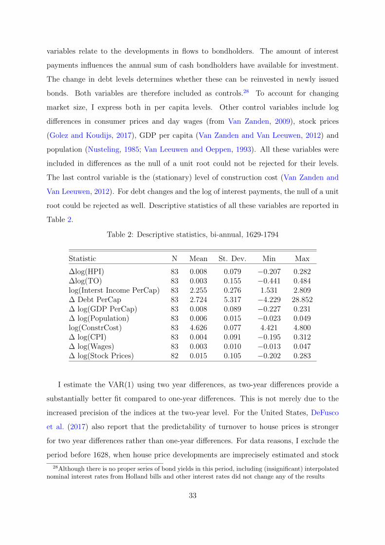
variables relate to the developments in flows to bondholders. The amount of interest

payments influences the annual sum of cash bondholders have available for investment.

The change in debt levels determines whether these can be reinvested in newly issued

bonds. Both variables are therefore included as controls.28 To account for changing

market size, I express both in per capita levels. Other control variables include log

differences in consumer prices and day wages (from Van Zanden, 2009), stock prices

(Golez and Koudijs, 2017), GDP per capita (Van Zanden and Van Leeuwen, 2012) and

population (Nusteling, 1985; Van Leeuwen and Oeppen, 1993). All these variables were

included in differences as the null of a unit root could not be rejected for their levels.

The last control variable is the (stationary) level of construction cost (Van Zanden and

Van Leeuwen, 2012). For debt changes and the log of interest payments, the null of a unit

root could be rejected as well. Descriptive statistics of all these variables are reported in

Table 2.

Table 2: Descriptive statistics, bi-annual, 1629-1794

Statistic N Mean St. Dev. Min Max

∆log(HPI) 83 0.008 0.079 −0.207 0.282∆log(TO) 83 0.003 0.155 −0.441 0.484log(Interst Income PerCap) 83 2.255 0.276 1.531 2.809∆ Debt PerCap 83 2.724 5.317 −4.229 28.852∆ log(GDP PerCap) 83 0.008 0.089 −0.227 0.231∆ log(Population) 83 0.006 0.015 −0.023 0.049log(ConstrCost) 83 4.626 0.077 4.421 4.800∆ log(CPI) 83 0.004 0.091 −0.195 0.312∆ log(Wages) 83 0.003 0.010 −0.013 0.047∆ log(Stock Prices) 82 0.015 0.105 −0.202 0.283

I estimate the VAR(1) using two year differences, as two-year differences provide a

substantially better fit compared to one-year differences. This is not merely due to the

increased precision of the indices at the two-year level. For the United States, DeFusco

et al. (2017) also report that the predictability of turnover to house prices is stronger

for two year differences rather than one-year differences. For data reasons, I exclude the

period before 1628, when house price developments are imprecisely estimated and stock

28Although there is no proper series of bond yields in this period, including (insignificant) interpolatednominal interest rates from Holland bills and other interest rates did not change any of the results

33

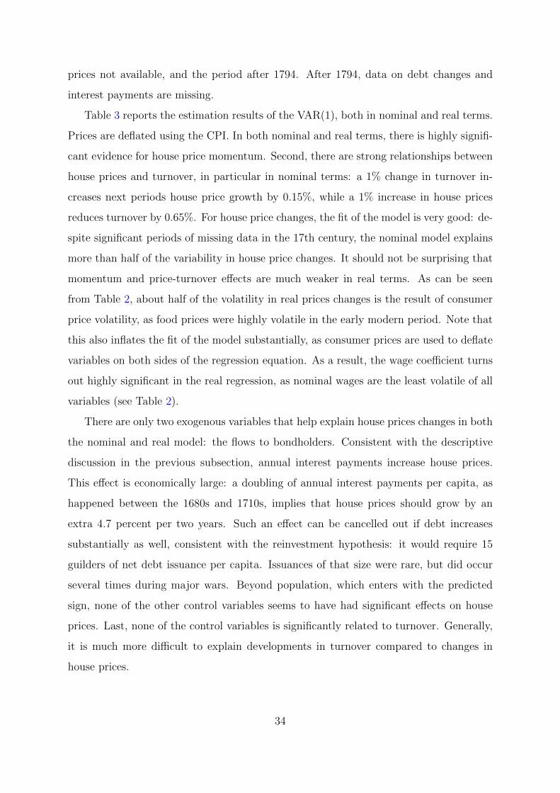
prices not available, and the period after 1794. After 1794, data on debt changes and

interest payments are missing.

Table 3 reports the estimation results of the VAR(1), both in nominal and real terms.

Prices are deflated using the CPI. In both nominal and real terms, there is highly signifi-

cant evidence for house price momentum. Second, there are strong relationships between

house prices and turnover, in particular in nominal terms: a 1% change in turnover in-

creases next periods house price growth by 0.15%, while a 1% increase in house prices

reduces turnover by 0.65%. For house price changes, the fit of the model is very good: de-

spite significant periods of missing data in the 17th century, the nominal model explains

more than half of the variability in house price changes. It should not be surprising that

momentum and price-turnover effects are much weaker in real terms. As can be seen

from Table 2, about half of the volatility in real prices changes is the result of consumer

price volatility, as food prices were highly volatile in the early modern period. Note that

this also inflates the fit of the model substantially, as consumer prices are used to deflate

variables on both sides of the regression equation. As a result, the wage coefficient turns

out highly significant in the real regression, as nominal wages are the least volatile of all

variables (see Table 2).

There are only two exogenous variables that help explain house prices changes in both

the nominal and real model: the flows to bondholders. Consistent with the descriptive

discussion in the previous subsection, annual interest payments increase house prices.

This effect is economically large: a doubling of annual interest payments per capita, as

happened between the 1680s and 1710s, implies that house prices should grow by an

extra 4.7 percent per two years. Such an effect can be cancelled out if debt increases

substantially as well, consistent with the reinvestment hypothesis: it would require 15

guilders of net debt issuance per capita. Issuances of that size were rare, but did occur

several times during major wars. Beyond population, which enters with the predicted

sign, none of the other control variables seems to have had significant effects on house

prices. Last, none of the control variables is significantly related to turnover. Generally,

it is much more difficult to explain developments in turnover compared to changes in

house prices.

34

Table 3: 2-year VAR regressions, 1610-1794

Dependent variable:

Nominal prices Real prices

∆log(HPI) ∆log(TO) ∆log(HPI) ∆log(TO)

∆log(HPI)−1 0.343∗∗∗ −0.727∗∗∗ 0.167∗∗ −0.267(0.092) (0.243) (0.065) (0.210)

∆log(TO)−1 0.147∗∗∗ −0.116 0.118∗∗∗ −0.115(0.044) (0.116) (0.036) (0.117)

Constant 0.498 −0.905 0.421∗∗∗ 0.384(0.567) (1.497) (0.142) (0.461)

log(IntInc) 0.069∗∗ 0.129 0.091∗∗∗ 0.083(0.032) (0.084) (0.031) (0.100)

DebtChange −0.003∗∗ −0.003 −0.032∗∗ −0.019(0.001) (0.003) (0.013) (0.042)

∆log(GDPcap) 0.125 0.001 0.158 −0.069(0.084) (0.223) (0.097) (0.314)

∆log(Pop) 1.247∗ 2.373 1.971∗∗∗ 1.864(0.677) (1.786) (0.544) (1.767)

log(ConstrCost) −0.141 0.132 −0.137 −0.096(0.117) (0.309) (0.089) (0.290)

∆log(CPI) −0.047 −0.016(0.091) (0.240)

∆log(StockPrices) −0.004 0.059 −0.029 0.168(0.067) (0.176) (0.066) (0.215)

∆log(Wages) 0.917 2.009 1.139∗∗∗ −0.286(0.848) (2.238) (0.125) (0.405)

Observations 82 82 82 82R2 0.527 0.138 0.778 0.056

Note: ∗p<0.1; ∗∗p<0.05; ∗∗∗p<0.01

35

4.2.1 Examining temporal variation

So far, I have implicitly assumed that the estimated coefficients should be fixed over

time. However, there are various reasons why there might be structural changes in the

estimated relationships. First of all, if dynamics between prices and turnover are driven

by speculative forces, they are likely much stronger during boom-bust cycles, when such

considerations play a more important role compared to ’quiet’ periods. Second, periods

with constrained housing supply, most notably during the first part of the 17th century,

might make house prices much more sensitive to changes in demand fundamentals. Third,

the impact of flows to bondholders on house prices might have changed with the size and

concentration of bond-holdings, as well as the availability of other investments. Last, from

a statistical point of view, measurement error might lead to noisy estimates in periods

where data is interpolated, in particular during the 17th century.

To examine temporal variation, I estimate VAR models over rolling windows of 50

years. The period of 50 years is substantially shorter than the full sample, but still leaves

sufficient observations (25 per window) to obtain significant coefficients. Also, the longest

house price cycles last about 50 years, such that one window can cover the entire cycle.

To reduce overfitting, I use the set of five nominal variables that leads to the highest

average adjusted R-squared: log differences in house prices, turnover and population, as

well as log interest rate income per capita, and net debt changes per capita. In addition, I

exclude the period before 1637, given that turnover data is entirely missing between 1632

and 1637. To get an indication how much of the momentum and price-turnover effects

might be due to persistence in flows to bondholders and population changes, I also report

unconditional rolling window-regressions (for these, I use the entire sample period).

Figures 8, 9, and 10 plot the coefficients of the rolling window regressions.29 The

year on the x-axis represents the median year in the rolling window sample, and the

thickness of the line indicates the significance: the thickest lines imply significance at the

5 percent level, while medium thickness represents significance at the 10 percent level.

For reference, the figures also report developments in house prices and turnover.

29Unconditional regressions for turnover are not reported, as these are virtually the same as theconditional ones

36

Figure 8: Rolling windows, house prices, no controls

1650 1700 1750

100

150

200

250

300

350

400

Bia

nnua

l Nom

inal

Inde

x (1

810=

100)

Lagged TurnoverMomentum

House PricesAdjusted R−squared

−0.

50.

00.

51.

0

Ela

stic

ity /

Adj

. R^2

Figure 9: Rolling windows, house prices, with controls

1660 1680 1700 1720 1740 1760

−0.

20.

00.

20.

40.

60.

8

Ela

stic

ity /

Adj

. R^2

Lagged TurnoverInterest (pc)MomentumDebt Change (pc)

Adjusted R−squared

−0.

010.

000.

010.

020.

030.

04

Effe

ct D

ebt C

hang

e (p

er c

ap)

37

Figure 10: Rolling windows, turnover, with controls

1660 1680 1700 1720 1740 1760

0.00

0.01

0.02

0.03

0.04

0.05

0.06

Turn

over

(2−

y A

VG

)

House PricesTurnoverLagged House Price Changes

−2

−1

01

Ela

stic

ity

The first panel panel shows that unconditional momentum effects are relatively stable

over time, and almost consistently present in the sample, in line with Table 1. Only in

the first half of the 17th century there do not seem momentum effects, but this is most

likely the result of measurement error in the indices. This might also explain why the

effect of lagged turnover on house prices is smaller in the 17th century, as turnover data is

often missing in this period. Generally, lagged turnover seems a strong predictor of house

prices, in particular during strong boom-bust cycles. If momentum effects and price-

turnover relationships are merely driven by speculation and sluggish responses of prices

to market conditions, we should not expect their effects to be modified by the inclusion

of control variables. While this seems to hold for the relationship between house prices

and turnover, it is not the case for house price momentum: Figure 9 shows that much of

the momentum effect results from the persistence in flows to bondholders, and to a lesser

extent from persistence in population changes, which are omitted in the figure.

Figure 9 also shows that flows to bondholders only became a significant factor at the

end of the 17th century, when interest payments had become increasingly important for

total liquidity, and other investment opportunities limited (De Vries and Van der Woude,

1997). However, as long as debt increased significantly, debt changes limited house price

growth: the significance of the change in debt levels coincides closely with the increases

38

in public debt presented in Figure 5. The combination of interest payments and changes

in public debt levels seems to particularly relevant for the windows that are centered

around the 1700s and 1710s, when none of the other variables enters significantly. This

supports the hypothesis that the take-off of the housing boom in the 1713-1739 period

can be attributed to the change in debt policy. Similar considerations seem important as

well around 1760, when the second large boom period starts.

For the rolling windows centered between 1720 and 1740, which cover the entire boom-

bust cycle, there is still significant evidence for momentum effects, together with positive

predictability of prices with turnover. Such dynamics are in line with house prices models

that include elements of optimism or speculation (Piazzesi and Schneider, 2009; DeFusco

et al., 2017). While the take-off of the boom might be attributed to debt policy changes,

speculative purchases might have helped to further inflate it, eventually resulting in a

very large bust when the government started borrowing again.

The persistence of the price-turnover effect for the remainder of the 18th century

also supports theories that assume sluggish adjustment of prices to changes in market

conditions (e.g. Berkovec and Goodman, 1996; Genesove and Han, 2012), as well as the

potential presence of loss aversion Genesove and Mayer (2001). It is not yet entirely

clear why the price-turnover effect persists almost the entire 18th century, while being

insignificant for most of the 17th century. Potentially, this is related to measurement

error in turnover before 1700.

As also evident from the fixed regressions in the previous subsection, turnover is

substantially less predictable than house prices. Generally, house prices negatively predict

changes in turnover, but these effects are highly variable over time and only significant

in a handful of cases. This contrasts to the predictability of house prices: despite the

simplicity of the model, it explains on average over half of the changes in house prices.

During the 18th century, the adjusted R-squared even increases to over seventy percent.

5 Conclusion

Our journey through the Amsterdam housing market has yielded several new insights.

House price booms and busts are nothing new under the sun: in this paper I have doc-

39

umented the existence of significant boom-bust cycles in Amsterdam in the pre-modern

era. Although the organization and financing of the Amsterdam housing market was dif-

ferent compared to modern markets: there were no fiscal benefits to home-ownership, the

mortgage market was small to non-existent, and explicit monetary policy did not yet ex-

ist. Despite the absence of these factors, Amsterdam went through three large boom-bust

cycles which were characterized by the same features as those in modern markets: mo-

mentum in house prices, excess volatility of prices relative to fundamentals but reversion

over the longer run, and a price-turnover relationship. This suggests, somewhat paradox-

ically, that booms and busts might be ’fundamental’ to the nature of housing markets:

although housing cycles might each have very different reasons, they have occurred as far

as historical data can stretch.

The absence of mortgage markets for most of the boom-bust cycles has important

implications for current debates. Inspired by the recent US housing bubble, much of the

literature has focused on whether changes in mortgage credit can help to generate boom-

bust cycles, and it is beyond doubt that such considerations are relevant. However, the

case of Amsterdam shows that mortgage credit booms are not a necessary condition for

large housing booms to appear. This implies we should also be concerned about housing

booms when mortgage credit is not expanding. This becomes particularly relevant in

relation to the main cause of the 1713-1739 boom identified in this paper: excess liquidity.

When Holland debt did not expand anymore, bondholders received large amounts of cash

interest payments that they could not save in Holland bonds. Much of this was invested

in Amsterdam real estate, and it did nothing but inflating asset prices. Although 18th

century Amsterdam was still very different from the modern economy, we can draw some

parallels to current conditions. After the recent crisis, the combination of low interest

rates and unconvential monetary policy has led to large increases in the monetary liquidity

available for investment, while asset prices have increased substantially. Correspondingly,

much of the current surge in Amsterdam house prices (and in many other cities), has been

attributed to increased demand from investors who are looking for profitable investment

opportunities (e.g. Hekwolter et al., 2017). However, contrary to the 18th century, it

is much more difficult to identify the price effects of this increased demand, given the

endogeneity of monetary policy and the fact that house price developments are highly

40

connected to the state of the general economy. What the historical Amsterdam case

shows, is that such episodes are able to trigger large and prolonged increases in house

prices, which might eventually lead to a bust when conditions change.

This paper also has imported implications for the debate on the drivers of the price-

turnover relationship. My empirical findings indicate there are two components that

are possibly driving the price-turnover relationship in Amsterdam. First, house prices

respond sluggishly to demand, while turnover responds much quicker. This creates a lead-

lag relationship between turnover and house prices, which is strongest at the two year

level, consistent with Berkovec and Goodman (1996); Genesove and Han (2012); DeFusco

et al. (2017). Changes in turnover positively predict changes in house prices, while to a

lesser extent house price changes negatively predict future turnover. Second, the share of

short-term investors increases significantly during the initial phase of booms, which sug-

gests that speculators, potentially attracted to the market by predictable price increases,

might have helped to further build up house price booms and generate momentum effects,

as in Piazzesi and Schneider (2009) and DeFusco et al. (2017). This effect is most pro-

nounced during the boom and bust in the first half of the 18th century. The combination

of speculative investors with excess liquidity also relates to the findings of Mian and Sufi

(2018). In their paper, shocks in the supply of mortgages can induce speculation, which

together led to the bubble in US house prices in the 2000s. In this paper, the large cash

flows towards bondholders are the suggested trigger of speculation. However, in both pa-

per it is not possible to identify exactly how much speculators contributed to the boom.

Third, the absence of mortgage markets in Amsterdam indicate that models that build

on mortgage credit constraints, as in Stein (1995) and Ortalo-Magne and Rady (2006),

cannot account for the observed price-turnover relationship. Last, although beyond the

scope of this paper, it is also very well possible that loss aversion (Genesove and Mayer,

2001) or other forms of history dependence (Bracke and Tenreyro, 2016; Hong et al.,

2016) contributed to aggregate dynamics in prices and turnover.

There still remains one important, but highly sensitive issue that needs to be ad-

dressed: can these boom-bust cycles be classified as traditional bubbles? Of course, much

of the answer to this question depends on what we define as a bubble. Since the 18th

century, the traditional Dutch word for a bubble has been ’windhandel’, metaphorically

41

meaning that only wind is being traded (Leemans, 2017). Of course, the Amsterdam real

estate market was much more than ’wind’: despite strong booms and busts, most of the

variability in individual transaction prices was reflecting different housing quality rather

than changing market prices. However, based on rent-price and price-income ratios, Am-

sterdam prices provide strong indications for bubbles: house prices strongly diverted

from fundamentals during booms, but quickly reverted during busts. However, much of

these deviations have rational explanations. When bondholders could not reinvest their

accumulated wealth into government bonds, there were limited alternative investment

opportunities available. As a result, bondholders might have reduced their required re-

turn on alternative investments, implying that a simple change in the discount rate can

be responsible for most of the increase in prices. Over the long-term real estate might

have been considered a relatively safe investment: if homes were held long enough, the

received rental yields would likely exceed the money lost in a potential housing market

crash. This line of reasoning would also explain why deviations from rents and income

could last for such a long period of time: each of the housing cycles spanned about 40 to

50 years, much longer than modern cycles or bubbles.

Accordingly, increases in the number of speculative buyers provide the strongest evi-

dence for the existence of ’bubbly’ components in the boom-bust cycle between 1713-1750.

Some investors might have indeed realized that real estate was overvalued: McCants

(1997) describe how the Amsterdam Burgerweeshuis, the largest institutional investor,

did not make any investments in the real estate market after 1712, and started to shift

its asset portfolio towards financial securities (see also Gelderblom and Jonker, 2009). In

addition, the decline of 50 percent in gross rental yields must have at least pulled away

some investors from further real estate investments. However, despite these concerns,

investors continued to buy properties in the Amsterdam housing market, until the boom

went bust and prices reversed. Hence, the 1713-1750 cycle has at least some elements

that make it a contender for the title of ’earliest documented housing bubble’. Hopefully,

it does not keep that status for too long: there still is a wealth of historical real estate

data remaining to be explored in future research, and undoubtedly some of these might

help to improve our understanding of housing markets.

42

Archival Sources

Amsterdam City Archives, Archief van de Thesaurieren Extraordinaris (entry no. 5044).

Amsterdam City Archives, Archief van de Honderdste en Tweehonderdste Penningkamerof Commissarissen tot de Ontvangst van de Honderdste en Andere Penningen (entry no.5045).

Amsterdam City Archives, Archief van de Secretaris: stukken betreffende het toezicht opde ontvangst van de veertigste, tachtigste, twintigste penning en de hele en halve veer-tigste penning (entry no. 5047).

Amsterdam City Archives, Archieven van de Schout en Schepenen, van de Schepenen envan de Subalterne Rechtbanken (entry no. 5061).

Amsterdam City Archives, Archief van de Schepenen: kwijtscheldingsregisters (entry no.5062).

Amsterdam City Archives, Archief van de Schepenen: register van rentebrieven en vantransporten van los- en lijfrenten (entry no. 5065).

Amsterdam City Archives, Archief van de Schepenen: register van willige decreten vanhet Hof van Holland (entry no. 5066).

Amsterdam City Archives, Archief van de Schepenen: register van afschrijvingen bij dewillige decreten (entry no. 5067).

Amsterdam City Archives, Archief van de Weeskamer en Commissie van Liquidatie derZaken van de Voormalige Weeksamer (entry no. 5073).

Dutch National Archives, Archief van het Hof van Holland (entry no. 3.03.01.01).

Regional Archives Dordrecht, Oud-rechterlijk archief (entry no. 9)

References

Abrahamse, J. E. (2010). De grote uitleg van Amsterdam: stadsontwikkeling in de zeven-tiende eeuw. Thoth.

Ambrose, B. W., Eichholtz, P., and Lindenthal, T. (2013). House prices and fundamen-tals: 355 years of evidence. Journal of Money, Credit and Banking, 45(2-3):477–491.

Bailey, M. J., Muth, R. F., and Nourse, H. O. (1963). A regression method for real estateprice index construction. Journal of the American Statistical Association, 58(304):933–942.

43

Berkovec, J. A. and Goodman, J. L. (1996). Turnover as a measure of demand for existinghomes. Real Estate Economics, 24(4):421–440.

Best, M. C. and Kleven, H. J. (2017). Housing market responses to transaction taxes:Evidence from notches and stimulus in the UK. The Review of Economic Studies,85(1):157–193.

Bracke, P. and Tenreyro, S. (2016). History dependence in the housing market.

Burnside, C., Eichenbaum, M., and Rebelo, S. (2016). Understanding booms and bustsin housing markets. Journal of Political Economy, 124(4):1088–1147.

Campbell, S. D., Davis, M. A., Gallin, J., and Martin, R. F. (2009). What moveshousing markets: A variance decomposition of the rent–price ratio. Journal of UrbanEconomics, 66(2):90–102.

Carter, A. (1953). Dutch foreign investment, 1738-1800. Economica, 20(80):322–340.

Case, K. E. and Shiller, R. J. (1987). Prices of single-family homes since 1970: newindexes for four cities. New England Economic Review, (Sep):45–56.

Case, K. E. and Shiller, R. J. (1989). The efficiency of the market for single-family homes.The American Economic Review, 79(1):125.

Cau, C., van Leeuwen, S., Scheltus, J., Scheltus, P., and Scheltus, I. (1658). Groot placaet-boeck, vervattende de placaten, ordonnantien ende edicten van de door-luchtige, hooghmog. heeren Staten Generael der Vereenighde Nederlanden ende vande ed. groot-mog.heeren Staten van Hollandt en West-Vrieslandt, mits-gaders vande ed. mog. heerenStaten van Zeelandt, volume 1-9. Johannes Allart.

Clayton, J., Miller, N., and Peng, L. (2010). Price-volume correlation in the housingmarket. The Journal of Real Estate Finance and Economics, 40(1):14–40.

de Montesquieu, C. d. S. and de Montesquieu, A. (1894). Voyages de Montesquieu, publiespar le Bon Albert de Montesquieu. G. Gounouilhou.

De Vries, J. and Van der Woude, A. (1997). The first modern economy: Success, failure,and perseverance of the Dutch economy, 1500–1815. Cambridge University Press.

De Wit, E. R., Englund, P., and Francke, M. K. (2013). Price and transaction volume inthe Dutch housing market. Regional Science and Urban Economics, 43(2):220–241.

DeFusco, A. A., Nathanson, C. G., and Zwick, E. (2017). Speculative dynamics of pricesand volume. NBER Working Paper.

Del Negro, M. and Otrok, C. (2007). 99 Luftballons: Monetary policy and the houseprice boom across US states. Journal of Monetary Economics, 54(7):1962–1985.

Diaz, A. and Jerez, B. (2013). House prices, sales, and time on the market: A search-theoretic framework. International Economic Review, 54(3):837–872.

44

Dormans, E. H. M. (1991). Het tekort: staatsschuld in de tijd der Republiek. PhD thesis.

Droes, M., Houben, A., van Lamoen, R., et al. (2017). De prijsstijgingen op de amster-damse huizenmarkt onder de loep. Economisch-Statistische Berichten, 102.

Droes, M. I. and Francke, M. K. (2017). What causes the price-turnover correlation inEuropean housing markets? The Journal of Real Estate Finance and Economics, pages1–29.

Duon, G. (1946). Documents sur le probleme du logement. Etudes Economiques, (1):1–165.

Eichholtz, P. (1997). A long run house price index: The Herengracht index, 1628–1973.Real Estate Economics, 25(2):175–192.

Eichholtz, P. M., Korevaar, M., and Lindenthal, T. (2017). 500 years of housing rents,quality and affordability in European cities.

Faber, J. (1980). Inhabitants of amsterdam and their possessions. Probate Inventories:A New Source for the Historical Study of Wealth, Material Culture and AgriculturalDevelopment, pages 149–55.

Favara, G. and Imbs, J. (2015). Credit supply and the price of housing. AmericanEconomic Review, 105(3):958–92.

Favilukis, J., Ludvigson, S. C., and Van Nieuwerburgh, S. (2017). The macroeconomic ef-fects of housing wealth, housing finance, and limited risk sharing in general equilibrium.Journal of Political Economy, 125(1):140–223.

Fishback, P. V., Flores-Lagunes, A., Horrace, W. C., Kantor, S., and Treber, J. (2010).The influence of the home owners’ loan corporation on housing markets during the1930s. The Review of Financial Studies, 24(6):1782–1813.

Frehen, R. G., Goetzmann, W. N., and Rouwenhorst, K. G. (2013). New evidence on thefirst financial bubble. Journal of Financial Economics, 108(3):585–607.

Gallin, J. (2006). The long-run relationship between house prices and income: evidencefrom local housing markets. Real Estate Economics, 34(3):417–438.

Gallin, J. (2008). The long-run relationship between house prices and rents. Real EstateEconomics, 36(4):635–658.

Gelderblom, O. and Jonker, J. (2009). With a view to hold. the emergence of institutionalinvestors on the amsterdam securities market during the seventeenth and eighteenthcenturies. The Origins and Development of Financial Markets and Institutions, pages71–98.

Gelderblom, O. and Jonker, J. (2011). Public finance and economic growth: the case ofHolland in the seventeenth century. The Journal of Economic History, 71(1):1–39.

45

Gelderblom, O., Jonker, J., and Hup, M. (2017). Financing in Europe, chapter PublicFunctions, Private Markets: Credit Registration by Aldermen and Notaries in the LowCountries, 1500-1800. Number 6. Palgrave.

Genesove, D. and Han, L. (2012). Search and matching in the housing market. Journalof Urban Economics, 72(1):31–45.

Genesove, D. and Mayer, C. (2001). Loss aversion and seller behavior: Evidence fromthe housing market. The Quarterly Journal of Economics, 116(4):1233–1260.

Glaeser, E. L. (2013). A nation of gamblers: Real estate speculation and Americanhistory. American Economic Review, 103(3):1–42.

Glaeser, E. L., Gottlieb, J. D., and Gyourko, J. (2012). Can cheap credit explain thehousing boom? In Housing and the financial crisis, pages 301–359. University ofChicago Press.

Glaeser, E. L. and Nathanson, C. G. (2014). Housing bubbles. NBER Working Paper.

Glaeser, E. L. and Nathanson, C. G. (2017). An extrapolative model of house pricedynamics. Journal of Financial Economics, 126(1):147–170.

Golez, B. and Koudijs, P. (2017). Four centuries of return predictability. Journal ofFinancial Economics.

Han, L., Strange, W. C., et al. (2015). The microstructure of housing markets. Handbookof Regional and Urban Economics, 5:813–886.

Hekwolter, M., Nijsken, R., and Heeringa, W. (2017). De woningmarkt in de grote steden.Technical report, De Nederlandsche Bank.

Himmelberg, C., Mayer, C., and Sinai, T. (2005). Assessing high house prices: Bubbles,fundamentals and misperceptions. Journal of Economic Perspectives, 19(4):67–92.

Hoffman, P. T., Postel-Vinay, G., and Rosenthal, J.-L. (2000). Priceless markets: thepolitical economy of credit in Paris, 1660-1870. University of Chicago Press.

Hong, D., Loh, R., and Warachka, M. (2016). Realization utility and real estate.

Iacoviello, M. (2005). House prices, borrowing constraints, and monetary policy in thebusiness cycle. American Economic Review, 95(3):739–764.

Jaremski, M. and Wheelock, D. (2018). Banking on the Boom, Tripped by the Bust:Banks and the World War I Agricultural Price Shock.

Jorda, O., Schularick, M., and Taylor, A. M. (2015). Betting the house. Journal ofInternational Economics, 96:S2–S18.

Kahneman, D. and Tversky, A. (1979). Prospect theory: An analysis of decision underrisk. Econometrica: Journal of the Econometric Society, pages 263–291.

46

Karagedikli, G. and Tuncer, C. (2016). The people next door: Housing and neighbour-hood in Ottoman Edirne, 1734-1814. Economic History Society Annual Conference.

Kindleberger, C. P. and Aliber, R. (2003). Manias, panics, and crashes. Springer.

Knoll, K. (2017). Our Home in Days Gone By: Housing Markets in Advanced Economiesin Historical Perspective. PhD thesis, Freie Universitat Berlin.

Knoll, K., Schularick, M., and Steger, T. (2017). No price like home: Global house prices,1870-2012. American Economic Review, 107(2):331–53.

Knotter, A. (1987). Bouwgolven in amsterdam in de 17e eeuw. PMM Klep, J. Th.Lindblad, AJ Schuurman, P. Singelenberg, Th. Van Tijn (eds), Wonen in het verleden,17e–20e eeuw: Economie, politiek, volkshuisvesting, cultuur en bibliografie, pages 25–37.

Krainer, J. (2001). A theory of liquidity in residential real estate markets. Journal ofurban Economics, 49(1):32–53.

Leemans, I. (2017). Porquoi le vent?: How the concept of wind came to embody specu-lative trade in the Dutch Republic.

Liesker, R. and Fritschy, W. (2004). Gewestelijke financien ten tijde van de Republiek derVerenigde Nederlanden: Holland (1572-1795). Inst. voor Nederlandse Geschiedenis.

Ling, D. C., Ooi, J. T., and Le, T. T. (2015). Explaining house price dynamics: Isolatingthe role of nonfundamentals. Journal of Money, Credit and Banking, 47(S1):87–125.

Lourens, P. and Lucassen, J. M. W. G. (1997). Inwonertallen van Nederlandse steden ca.1300-1800. NEHA.

McCants, A. E. C. (1997). Civic charity in a golden age: orphan care in early modernAmsterdam. University of Illinois Press.

Mian, A. and Sufi, A. (2009). The consequences of mortgage credit expansion: Evidencefrom the us mortgage default crisis. The Quarterly Journal of Economics, 124(4):1449–1496.

Mian, A. and Sufi, A. (2011). House prices, home equity-based borrowing, and the ushousehold leverage crisis. American Economic Review, 101(5):2132–56.

Mian, A. and Sufi, A. (2018). Credit supply and housing speculation. Technical report,National Bureau of Economic Research.

Mills, J., Molloy, R., and Zarutskie, R. (2017). Large-scale buy-to-rent investors inthe single-family housing market: The emergence of a new asset class. Real EstateEconomics.

Novy-Marx, R. (2009). Hot and cold markets. Real Estate Economics, 37(1):1–22.

47

Nusteling, H. P. H. (1985). Welvaart en werkgelegenheid in Amsterdam, 1540-1860: eenrelaas over demografie, economie en sociale politiek van een wereldstad. BataafscheLeeuw.

Ortalo-Magne, F. and Rady, S. (2006). Housing market dynamics: On the contribution ofincome shocks and credit constraints. The Review of Economic Studies, 73(2):459–485.

Piazzesi, M. and Schneider, M. (2009). Momentum traders in the housing market: Surveyevidence and a search model. The American Economic Review, 99(2):406–411.

Raff, D., Wachter, S., and Yan, S. (2013). Real estate prices in Beijing, 1644 to 1840.Explorations in Economic History, 50(3):368–386.

Rajan, R. and Ramcharan, R. (2015). The anatomy of a credit crisis: The boom andbust in farm land prices in the united states in the 1920s. American Economic Review,105(4):1439–77.

Reinhart, C. M. and Rogoff, K. S. (2009). This time is different: Eight centuries offinancial folly. princeton university press.

Rooseboom, G. (1656). Recueil van verscheyde keuren, en costumen: Midtsgadersmaniere van procederen binnen de stadt Amsterdam. Ian Hendricks.

Ryckbosch, W. (2016). Economic inequality and growth before the industrial revolution:the case of the Low Countries. European Review of Economic History, 20(1):1–22.

Schnabel, I. and Shin, H. S. (2004). Liquidity and contagion: The crisis of 1763. Journalof the European Economic Association, 2(6):929–968.

Shiller, R. J. (2015). Irrational exuberance: Revised and expanded third edition. Princetonuniversity press.

Sommer, K. and Sullivan, P. (2018). Implications of us tax policy for house prices, rents,and homeownership. American Economic Review, 108(2):241–74.

Sommer, K., Sullivan, P., and Verbrugge, R. (2013). The equilibrium effect of fundamen-tals on house prices and rents. Journal of Monetary Economics, 60(7):854–870.

Stein, J. C. (1995). Prices and trading volume in the housing market: A model withdown-payment effects. The Quarterly Journal of Economics, 110(2):379–406.

Temin, P. and Voth, H.-J. (2004). Riding the south sea bubble. American EconomicReview, 94(5):1654–1668.

Van Bochove, C., Boerner, L., and Quint, D. (2017). Anglo-Dutch premium auctions ineighteenth-century Amsterdam. SSRN Working Paper.

Van Bochove, C., Deneweth, H., and Zuijderduijn, J. (2015). Real estate and mortgagefinance in England and the Low Countries, 1300–1800. Continuity and Change, 30(1):9–38.

48

Van Bochove, C. and Kole, H. (2014). Uncovering private credit markets: Amsterdam,1660-1809. Tijdschrift voor Sociale en Economische Geschiedenis, 11(3):39.

Van Iterson, W. (1939). Willig Decreet in Holland en Utrecht. Tjeenk Willink, Haarlem.

Van Leeuwen, M. H. and Oeppen, J. E. (1993). Reconstructing the demographic regimeof amsterdam 1681–1920. Economic and Social History in the Netherlands, 5:61–102.

Van Wassenaer, J. H. (1737). Amsterdamsche Secretary. Gerrit Bos.

Van Zanden, J. L. (2009). Prices and wages and the cost of living in the western part ofthe Netherlands, 1450-1800. Website Historical Prices and Wages, IISH, 11.

Van Zanden, J. L. and Van Leeuwen, B. (2012). Persistent but not consistent: Thegrowth of national income in Holland 1347–1807. Explorations in Economic History,49(2):119–130.

Wagenaar, J. (1767). Amsterdam, in zyne opkomst, aanwas, geschiedenissen, voorregten,koophandel, gebouwen, kerkenstaat, schoolen, schutterye, gilden en regeeringe. IsaakTirion.

Wetzer, T. (2018). Bossche encyclopedie. https://www.bossche-encyclopedie.nl/.

White, E. N., Snowden, K., and Fishback, P. (2014). Housing and mortgage markets inhistorical perspective. University of Chicago Press.

Winkler, W. E. (1999). The state of record linkage and current research problems. InStatistical Research Division, US Census Bureau. Citeseer.

49

Appendix A: Example of act with transcription

Figure 11 contains an example of an ordinaris kwijtschelding, which formed the main bulk

of data. The form was standardized. This particular example relates to the purchase of

property by Rembrandt Hermansz, the well-known painter, from the heirs of Pieter Bel-

tens de Jonge. The (approximate) transcription contains in bold the data that is also

included in the digitalized dataset.

Figure 11: Property transfer act, ACA 5062, inv. nr. 45, page 195v

Transcription:

In margin: sold for fl. 13000

We, Cornelis van Vlooswijck and Gerrit van Hellemont, alderman in Amsterdam, write

50

and acknowledge that for us have appeared Christoffel Thys and Jan Beltens as heirs

of Pieter Beltens de Jonge, and have sold and remitted to Rembrandt Hermansz

a house and yard standing on the Breestraat, over the Sint Anthonis sluice, on

the west-side, with a free exit or pass-through to the house of Claes Elias, as has been

explained in the acts of remittance about those, and this being the house and yard that

is or was next to that of Claes Elias, with the entire wall on the north west side and that

of Salvador Rodrigues on the south east side, and reaches from the street until the house

and yard that belongs to Bastiaen Jacobsz Kistemaecker. And those that have appeared

have already committed to the terms, and the principal has brought Isaac van Beecq and

Dirck Dircks Grijp (jointly appeared) as joint guarantors, and each has promised with all

their movable property that this house and yard has and will be remitted year and day,

as one has promised to do, and to remove older acts. This is what the sellers have each

promised, and the principal has also promised to keep the guarantors free from losses

under the agreements written above. Entered January 8, 1653.

Appendix B: Procedure to find repeat-sales and esti-

mate turnover

Identifying repeat-sales

This procedure outlines the three steps taken to identify repeat-sales pairs. In the first

step, I aim to identify transaction pairs based on the names of buyers and sellers. The

name of the original owner is always mentioned on each transaction, even if her or she is

deceased, so a seller should have been listed as a buyer in an earlier recorded transaction,

as long as the home has been transacted previously and the register is not missing. To

reduce the number of potential matches, I search for buyers and sellers with the same

name (and sell date after buy date) for each street separately. Streets were likely always

entered correctly, and could only change if a home on a corner changed its main door to

face the other street, which would indicate a renovation and should therefore be excluded

anyhow. There are four caveats here. First of all, names might not be spelled exactly

the same due to errors in the transcriptions or registrations, or because a person did not

51

tell exactly the same name on both occasions. Second, multiple persons can share the

same name. Third, a person might have owned multiple properties on the same street.

Fourth, a property might have changed in quality

To avoid missing matches or making errors, I sort names alphabetically for each

street, and compute for each person the Jaro-Winkler distance (Winkler, 1999) with the

two persons around it in the list. The p-value is set at 0.1.

A pair is matched automatically in case the following four conditions hold. First, the

buyer and seller should have JW-distace of less than 0.1 for both the first name and the

last name. Second, the sale should take place after the purchase. Third, there should

be not other buyer and seller on the street with a similar name. This is identified by

examining the surrounding names. If any of these has a JW-distance of less than 0.15 for

both first name and last name, no match is made. Fourth, the type of property that is

being sold should be the same. Although no detailed quality information is available, the

sale acts list what type of good is being sold, such as land, house and land, warehouse

and land, shipyard etc. This avoids large quality changes among repeats.

In the second step, I re-evaluate the data that was excluded from matching in case

there was a buyer or seller with potentially the same name. I check all these cases by

hand, making use of various sorting mechanisms. Although this is very time consuming, it

is usually possible to verify based on the information about names, location and property

description whether two observations are a match or not. In case there is any reason for

doubt, no match is made.

In total, this lengthy procedure resulted in 72,544 repeat-sales, which is about 44%

of the total number of transactions. Of these 72,544 repeat sales, 68,143 have a positive

price and 67,295 involve residential property. Beyond data errors, there are three reasons

why it id not possible to match all transactions. First of all, due to missing registers in

the 16th and 17th century, the initial purchase or subsequent sale do not always show up

in the dataset. Second, many homes were never sold or sold only once during the period

covered by my dataset. Last, it is typically close to impossible to match transactions

where buyer or seller have very common names, such as ”Jan Jansz” (John Johnson).

52

Estimating turnover

The construction of a turnover index requires estimates of both the number of homes

transacted in each year, as well as the total number of homes in the city. To start with

the first, I identify for each transaction the number of homes that is involved; most

transactions are for one home, but partial sales or multiple sales occur frequently as well.

For transactions which combine residential and non-residential sales, only the residential

part is counted. Subsequently, I adjust for periods with missing data. Since the registers

were chronological, data is either complete or entirely missing. If a missing register does

not cover an entire year, and more than three months of data is still available for that

year, I estimate annual turnover by dividing the total number of transactions in these

months by the share of transactions that on average occur in these months. No estimates

of turnover are made for the ordinaris kwijtscheldingen prior to 1582, due to lack of data.

Data from orphan sales are excluded, as it does not represent the buying and selling

behavior from property owners, but rather the management of the orphan chamber.

In the last step, each of the series is scaled by the size of the market. Such a step is

necessary, as the city of Amsterdam expanded significantly in size during the 16th and

17th century. Tax registers reveal that from the 1680s, the size of the city and number

of homes stayed constant. In this period, there are in total around 25,000 properties in

the city, of which about 90% is assumed to contain residential real estate.30 It is more

difficult to obtain estimates on the number of homes prior to 1680, when Amsterdam

expanded significantly in size and had very large suburbs, which were rarely included

in the tax records. I therefore rely on existing estimates of the Amsterdam population

from Nusteling (1985) and Van Leeuwen and Oeppen (1993), and scale these based on

estimates of the number of people per home. For 1680, I assume the number of people

per home was equal to the number obtained from the tax records of 1733 (9.4 people

per home). Before 1632, it is set at 8.42 based on the number of homes reported in

Lourens and Lucassen (1997). Between 1632 and 1680, the number of people per home

is interpolated linearly.

30Source: ACA 5044, inv. nrs. 402-405

53

Appendix C: Locality of price developments

Beyond Amsterdam, house price records have also been digitized for Dordrecht and Den

Bosch. Records of these are publicly available from the Regional Archives of Dordrecht

and Wetzer (2018). These two cities, with average populations of respectively 18,000 and

15,000, were among the largest cities in the Republic between 1600-1800, and located

within 100 kilometers of Amsterdam. I will use these records to compare price develop-

ments in Amsterdam to other cities in the Republic. For Dordrecht, data is completely

available between 1683-1703, and 1730-1773. In total, there are 6785 sales in this period.

For Den Bosch, there are registrations of 11,489 transactions, between 1650-1672 and

1692-1838.

Figure 12 reports house prices in Amsterdam relative to bi-annual indices of house

prices in Dordrecht and Den Bosch. Note that due to the low number of data points,

the precision of these indices is smaller compared to Amsterdam, 31 but long-term trends

still stand out clearly.

Figure 12: House prices in Amsterdam, Den Bosch and Dordrecht

1650 1700 1750 1800

5010

015

020

0

Nom

inal

Inde

x (1

750=

100)

AmsterdamDordrechtDen Bosch

Interestingly, neither Den Bosch nor Dordrecht seem to have experienced the large

house price cycle that occurred in Amsterdam between 1713-1750. Prices declined in

31the average standard error of the bi-annual index is about 0.06 for both cities, relative to 0.025 forthe annual Amsterdam index

54

Den Bosch, and did not move much in Dordrecht, although data is missing between

1706-1730. During the second cycle, prices also increased substantially in Den Bosch

and Dordrecht, although with a substantial delay, in particular for Den Bosch. It might

be that the housing boom only spread gradually to other, less important cities, as has

also been observed in modern markets. Unsurprisingly, the fall in prices in the 1790s

and early 1800s was common to both Amsterdam and Den Bosch: the French period is

widely considered as the crisis that ended the important position of the Dutch Republic.

However, more general, it seems that house price cycles, in particular their exact timing,

is highly local. This also implies that we should look in detail at developments in local

housing markets to understand exactly why prices are going up or down.

Because this paper focuses on Amsterdam, a detailed look and explanation for price

developments in Den Bosch and Dordrecht is beyond its scope. However, both cities

seem to experience booms that did not appear in Amsterdam: Dordrecht in the late

17th century, and Den Bosch in the early 18th century. The latter boom is particularly

significant, and coincides with the War of the Spanish Succession. It might be that

investors speculated that Den Bosch, being the most important city in Dutch Brabant,

would gain a more important status within the Republic as the allied forces, including the

Republic, had conquered the Spanish Netherlands. Although this explanation requires

more detailed investigation, it might also explain why prices went down towards the end

of the war: following the Peace of Utrecht, the Spanish Netherlands went to Austria, and

the Republic barely gained any territory.

Appendix D: Developments in registered loan values

Figure 13 plots the developments in house prices relative to the total amount of non-

mortgage credit (credit without kusting) registered with the aldermen in Amsterdam.

To construct the latter series, I used payment registers of the tax on registered loans,

available between 1682-1805.32 Note that from the 1780s, notarial loans and private non-

registered also start to appear in the tax registers. Creditors and debtors likely voluntary

paid the tax on these loans in order to increase the seniority of the loan in case of default.

32Source: ACA 5047

55

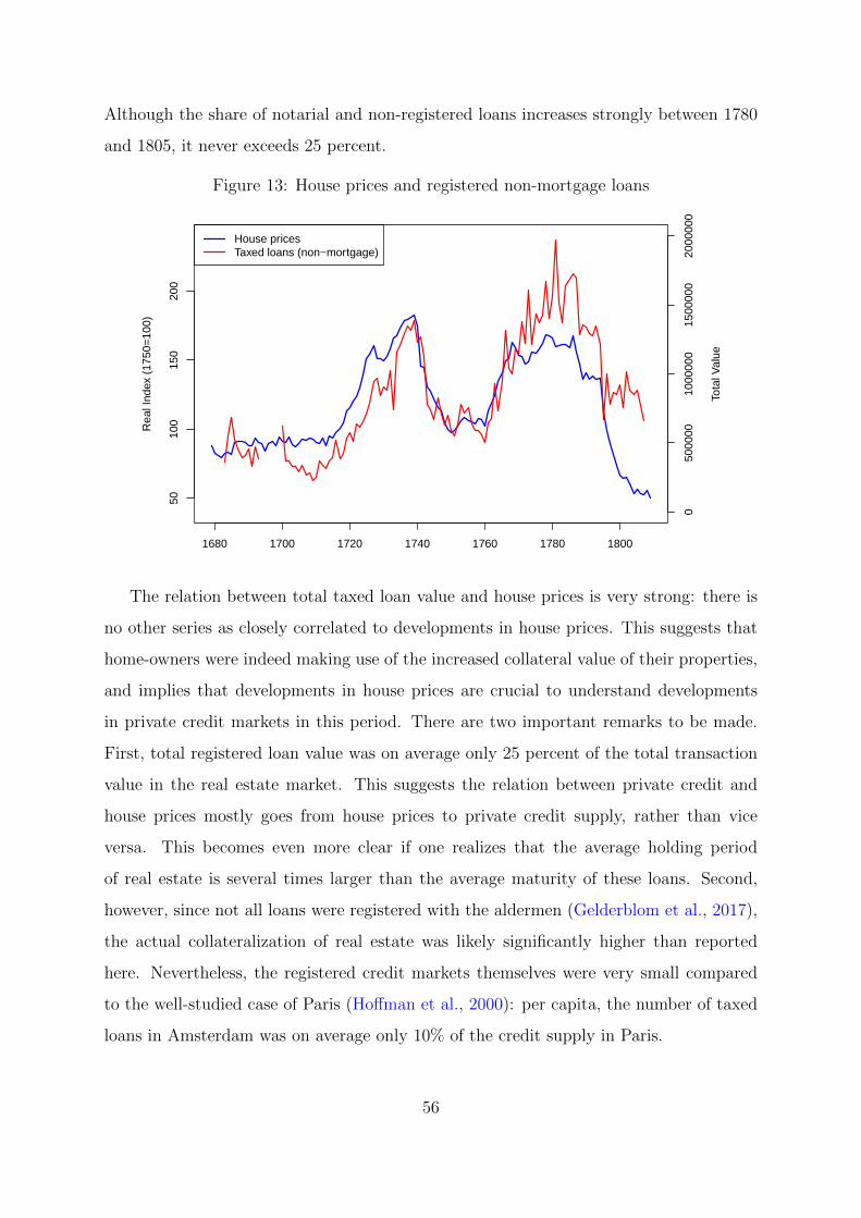
Although the share of notarial and non-registered loans increases strongly between 1780

and 1805, it never exceeds 25 percent.

Figure 13: House prices and registered non-mortgage loans

1680 1700 1720 1740 1760 1780 1800

5010

015

020

0

Rea

l Ind

ex (

1750

=10

0)

House pricesTaxed loans (non−mortgage)

050

0000

1000

000

1500

000

2000

000

Tota

l Val

ue

The relation between total taxed loan value and house prices is very strong: there is

no other series as closely correlated to developments in house prices. This suggests that

home-owners were indeed making use of the increased collateral value of their properties,

and implies that developments in house prices are crucial to understand developments

in private credit markets in this period. There are two important remarks to be made.

First, total registered loan value was on average only 25 percent of the total transaction

value in the real estate market. This suggests the relation between private credit and

house prices mostly goes from house prices to private credit supply, rather than vice

versa. This becomes even more clear if one realizes that the average holding period

of real estate is several times larger than the average maturity of these loans. Second,

however, since not all loans were registered with the aldermen (Gelderblom et al., 2017),

the actual collateralization of real estate was likely significantly higher than reported

here. Nevertheless, the registered credit markets themselves were very small compared

to the well-studied case of Paris (Hoffman et al., 2000): per capita, the number of taxed

loans in Amsterdam was on average only 10% of the credit supply in Paris.

56