THE "FLOWING" ACCUMULATION METHOD AND ITS APPLICATION 1!'OR EARTH SURFACE ANALYSIS

Yaroslav V. Golda

Research Scientist, Ternopil State Pedagogical Institute, ISPRS Commission IV.

ABSTRACT:

Method for the description of functions of two variables is proposed. Applications and interpretations are considered on the example of the analysis of the earth surface se~ mente Input data for computer processing is digital elevation model /DEM/ which is set at regular grid and obtained with a help of an automatized photogrammetrical device.

The DEM is described as a grqph. Every point of the DEM univocally responds to the on­ly node of the graph and vice verse. An arc indicates the direction of a maximum decr~ ase in the corresponding point of the DEM. The graph constructed in such a way consis~ of the directed trees. The quantitative functions which serve as integral characteris­tics of the surface are built on the nodes of the graph.

Algorithms worked out on the basis of this model provide for the following: - to carry out preliminary processing of the DEM with the purpose of recovering of the

surface structure adequate to the real one; - to describe a network of valleys thalvegs and borders of their drainage basins, to

define their structure; - to calculate the areas of the drainage basins, the length of thalvegs sections and

basins borders, etc.

The model can be used as a basis for the algorithms construction for automation of mop­phometrical analysis, the flowing calculations, water erosion processes investigation, topomaps processing.

KEY WORDS: DEM, Algorithm, Accuracy, Mapping, Image Interpretation.

1. INTRODUCTION

The method has been established and used as an attempt for solving a number of tasks ocurred when the processes of aeri­al photographs interpretation were auto­matized (Antoshchenko-Olenev and Golda, 1986). Both static relief and image terra in models are analysed while interpretin~ Geological objects are manifested in the structure of both the image model and the stereo one. Relief of the earth surface keeps footprints of atmosphere and hydro­sphere influence on geological environ­ment, as well as processes which have ta­ken place in it. Those "tracks" are coded in relief morphology characteristics. To calculate the morphology characteristics it's necessary to have a technique of surface description which would allow to derive automatically slopes, sceleton li­nes /thalvegs and watersheds/, to inves­tigate their topography and topology ha­ving only the DEM as input data.

Horton (1945), Strahler (1952), Shreve (1966) showed that development of channe~ networks and their drainage basins submi~ definite laws and drainage networks are described with the branched structures which have strictly definite hierarchy and topology. However, usually either si~ pIe differentiatio~ or more complicated constructions of differential geometry technique are used at attempts to automa­te process of sceleton lines derivation from topography surface. The ground of such approach is given in a paper of An­tipov and Kireytov (1979).

Analysis of that problem (Golda and others 1986) showed that it's impossible to cre­ate robust noise immunity algorithms of

836

sceleton lines recognition using only dif­ferential geometry methods. Firstly, it's because of technical reasons. We must use derivatives to second order including in calculations, i.e. quantitative implemen­tation needs both interpolation technique and input data of high quality. But nume­rical differentiation is less precise ope­ration than interpolation, that's why the result becomes dependent on interpolation technique and it's not noise immunited. Secondly, of intuition consideration. To construct a numerical model of drainage network it isn't sufficient to state the belonging of the points of the surface to thalvegs. It's necessary to connect these points into branched structures that sug­gest turning back to the input surface analysis. The researcher does not consi­der the picture of the infinitely small surface segments when quoting thalvegs on the topomap, he observes it in the whole. He can decide if the point belongs to the thalveg only taking into consideration the surface curving "up the flowing" and information about the drainage area, and he can make up watersheds on the surface having a knowledge of the framework of the channel network. Hence, formal proce­dures of sceleton lines derivation cannot be based only on the surface shape rese­arch. It's obligatory to define the sur­face directly as a structure drawing at­tention to integral characteristics which allow to judge of the grade of substrat "washing up" by water erosion or of the level of relief developing.

2. MATHEMATICAL MODEL

2.1. The Description of the Surface

For surface description we use mathemati­cal model, which is one of the consequen­ces of "flowing" accumulation method pro­posed by the author before. We consider a surface Z(X,Y) as a discrete function of two variables Z(Xi,Yj), i.e. two-dimensi­onal array of heights Zron corresponding to knots of quadrangle grid (i,j},i=~,M] j=[1,N]. {i,j} is a set of knots where the surface is determined. We describe the surface as a graph, nodes of which are put on the same {i,j} set. Eacll node of a graph is put bijectically to the on­ly point of the surface. Arcs of the~ €,?;J;'aph are defined as the mapping P({i', j}) that is linear chained list groupped in matrix of links Pron.

if function

i.:: [2 ,M-i]

J= [2,M-1) k=i:-1,lJH

[==j-1,j,j+1

reaches its minimum at k=k, 1=1. p(i,j) value points direction of maximumdecrea­se of Z(X,Y) in (i,j) knot /neighbouring point on the surface/. Therefore, the graph G({i,jl,Pmn) built in such a way is a forest consisting of directed trees with reverse orientation of arcs. According to the construction, no more than one arc co­mes off from each node. A node that does not receive any arc is a leaf. A node from which none of arcs comes off is a root. We call path from leaf to root a flowinglin-e. A (i,j)node is a root of a tree if p(i,j)=(i,j) i.e. functionZ(X,Y) reaches its local minimum at Z(X·,~ ) pOint. As for i:1,M; j=1,N p(i,j~ values are not determined, the corresponding no­des are roots as well.

We call reflexive closure of any node (k,l), i.e. the set of nodes from which there exist paths to the given node (k,l) as flowing accumulation are~ of (k,l)node /(k,l) FAA/. The boundary 6f this set on {i,j} may be named as the (k,l)FAA boun­dary. The segment of Z(X,Y) which is map­ped into (k,l)FAA is called Ahe drainage basin of Z(Xt, Yj) surface point /Z(Xt,Yj)DB/, and its boundary on the surface is called Z(Xt'YJ )DB boundary.

According to the G({i,j},Pmn) constructi­on nodes of each separated tree make clo­sed one~chained domain on {i,j}. Domains formed of ·different trees nodes do not join. Each domain is a projection of DB, and its boundary is a projection of DB boundary of the surface point correspon­ding to the root.

837

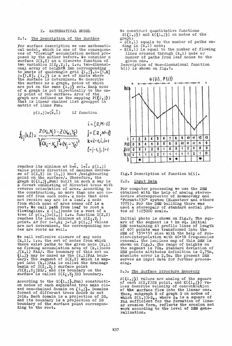
We construct quantitative functions S({i,j}) and K({i,j}) on nodes of the

graph: - S(k,l) equals to the number of paths en­

ding in (k,l) node; - K(k,l) is equal to the number of flowing

lines crossed through (k,l) node or number of paths from leaf nodes to the given one.

Description of Qne-dimensional function h(i) is shown on fig.l.

G({L), PH}) o ~ 0---0---0--0--0 0

1

f1" ~

1\ V h

1\ V 1\ IV f\ V N

f 2 3 4 S G 7 & 9 iO 11 12

) 0 5 .. 5 5 5 6 9 iO it 11 11

') 0 0' f 2 5 i 0 tl 4 2 .. 0

i} 0 1 1 1 2 1 1 i 1: 1 2. 1

• *' * • fig.i Description of function h(i).

2.2. Input Data

I

V

~3

0 0

0

For computer processing we use the DEM obtained with the help of analog stereo­device stereoproector of Romanovsky and ItFormat-130" system (Kuznetsov and others 1979). For the DEM building there was used a stereopair of standard aerial pho­tos of 1:25000 scale.

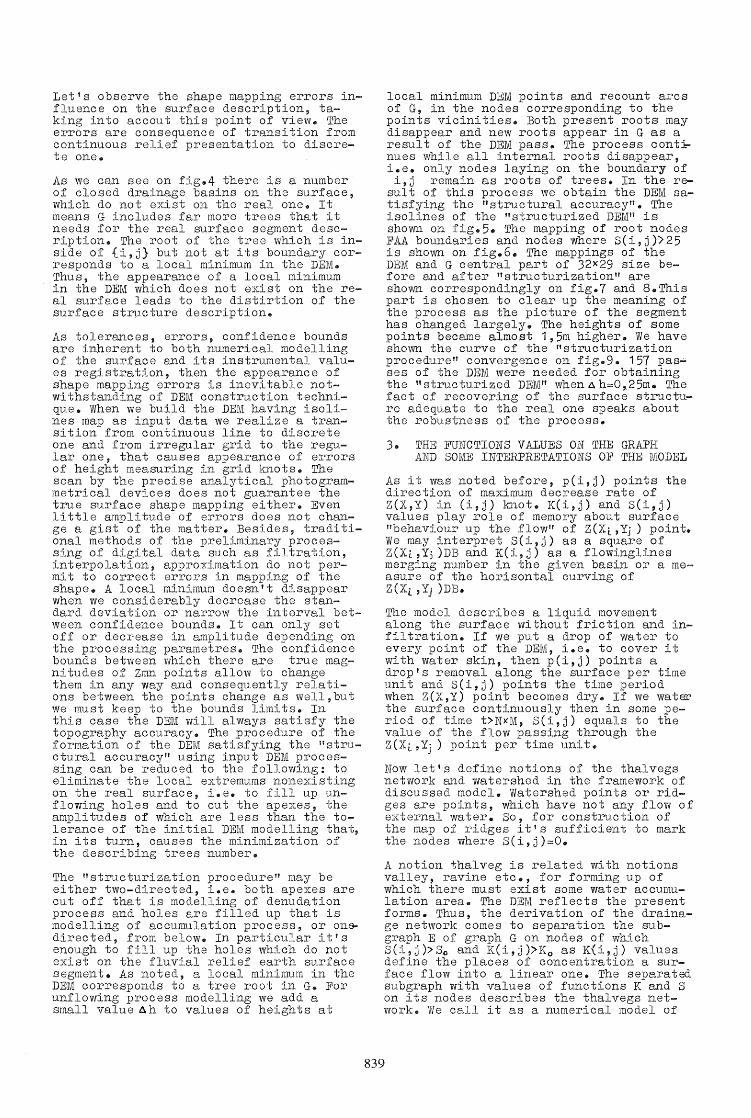
Initial photo is shown on fig.2. The squ­are of the segment is 1 km sq. Initial DEM containing 41 profile lines of length of 401 points was transformed into the DEM of 151x151 size with the help of Fou­rier-interpolation with 40 x 18 frequencies renewal. The isolines map of this DEM is shown on fig.3. The range of heights on the segme~t is 70m. Standard deviation of DEM points altitudes definition is O,75m, absolute error is 2,5m. The present DEM serves as input data for further proces­sing.

2.3. The Surface Structure Recovery

S({i,j}) values are analog of the square of each Z(X,Y)DB point, and K({,i,j}) va­lues describe velocity of concentration of the .surface flow into the linear one. Thus, sub graph E of graph G on nodes of which S(i.j»So, where So is a square of FAA sufficient for the formation of line­ar erosion form, reflects the erosi9n net work according to the level of DEM gene­ralization.

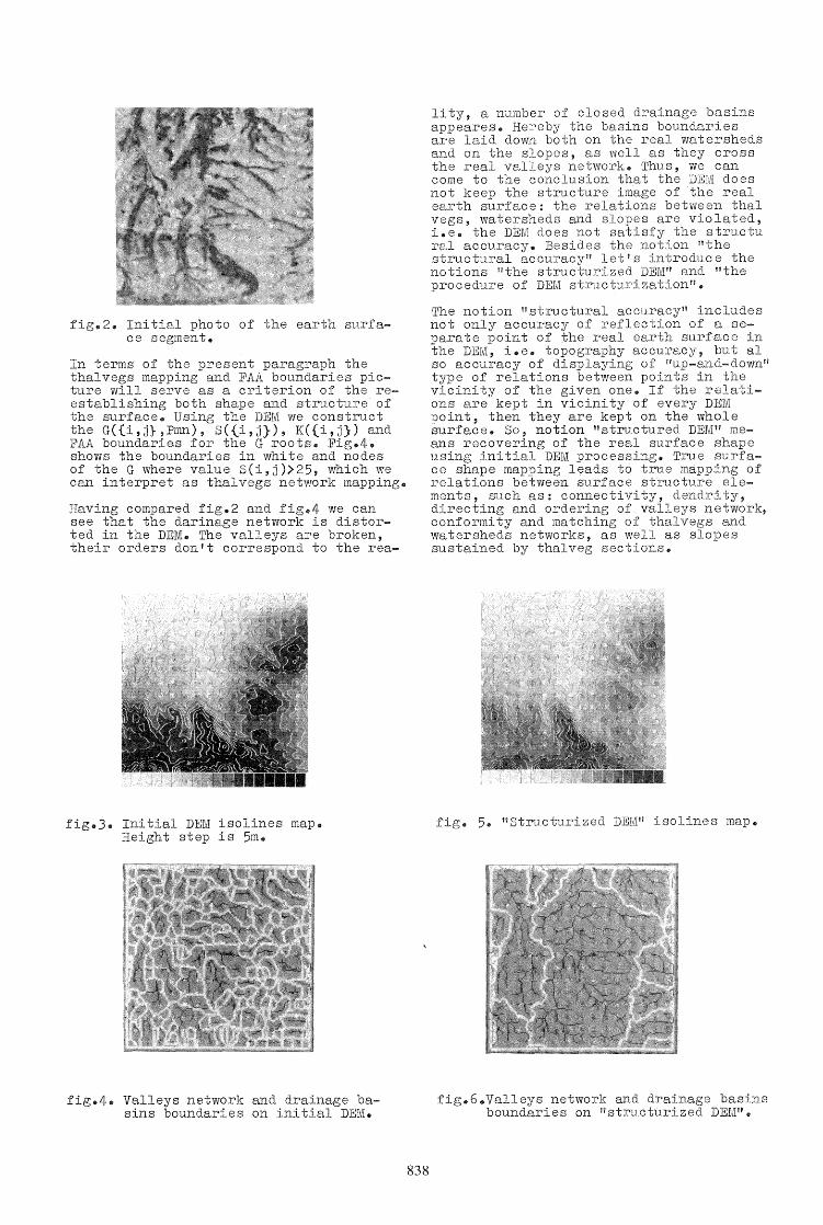
2. Initial photo of the earth surfa­ce segment.

In terms of the present paragraph the thalvegs mapping and FAA boundaries pic­ture will serve as a criterion of the re­establishing both shape and structure of the surface. Using the DEM we construct the G({i,j},Pmn), S({i,j}), K({i,j}) and FAA boundarie.s for the G roots. :Pig.4. shows the boundaries in white and nodes of the G where value S(i,j»25, which we can interpret as thalvegs network mapping.

Having compared fig.2 and fig.4 we can see that the darinage network is distor­ted in the DEM. The valleys are broken, their orders don't correspond to the rea-

3. Initial DEllII isolines map. Height step is 5m.

fig.4. Valleys network and drainage ba­sins boundaries on initial DEM.

838

lity, a number of closed drainage basins appeares. Hereby the basins boundaries are laid dovID both on the real watersheds and on the slopes, as well as they cross the real valleys network. Thus, we can come to the conclusion that the DEM does not keep the structure of the real earth surface: the relations between thal vegs, watersheds and slopes are violated, i.e .. the DBM does not satisfy the structu ral accuracy. Besides the notion "the structural accuracy!! let's introduce the notions llthe structurized DEMIT and "the procedure of DEM stru.cturization f' ..

The notion llstructural accuracy" includes not only accuracy of reflection of a se­parate point of the real earth surface in the DEM, i.e. topography accuracy, but al so accuracy of displaying of "up-and-down ll

type of relations between points in the vicinity of the given one. If the relati­ons are kept in vicinity of every DEM point, then they are kept on the whole surface. So~ notion "structured DErvr H me­ans recovering of the real surface shape using initial DEM processing. True surfa­ce shape mapping leads to trI.:le mapping of relations between surface structure ele­ments, such as: connectivity, dendrity, directing and ordering of valleys network, conformity and matching of thalvegs and watersheds networks, as well as slopes sustained by thalveg sections.

5. nstructurized DEMiI isolines map ..

fig.6.Valleys network and drainage basins boundaries on llstructurized DEM".

Let's observe the shape mapping errors in­fluence on the surface description, ta­king into accout this point of view. The errors are consequence of transition from continuous relief presentation to discre­te one.

As we can see on fig.4 there is a number of closed drainage basins on the surface, which do not exist on the real one. It means G includes far more trees that it needs for the real surface segment desc­ription. The root of the tree which is in­side of {i,j} but not at its boundary cor­responds to a local minimum in the DEM. Thus, the appearance of a local minimum in the DEM which does not ey~st on the re­al surface leads to the distirtion of the surface structure description.

As tolerances, errors, confidence bounds are inherent to both numerical modelling of the surface and its instrumental valu­es registration, then the appearance of shape mapping errors is inevitable not­withstanding of DEM construction techni­que. When we build the DEM having isoli­nes map as input data we realize a tran­sition from continuous line to discrete one and from irregular grid to the regu­lar one, that causes appearance of errors of height measuring in grid knots. The scan by the precise analytical photogram­metrical devices does not gu.arantee the tr1..le surface shape mapping either. Even little amplitude of errors does not chan­ge a gist of the matter. Besides, traditi­onal methods of the preliminary proces­sing of digital data such as filtration, interpolation, approximation do not per­mit to correct errors in mapping of the shape. A local minimum doesn't disappear when we considerably decrease the stan­dard deviation or narrow the interval bet­ween confidence bounds. It can only set off or decrease in amplitude depending on the processing parametres. The confidence bounds between which there are true mag­nitudes of Zmn points allow to change them in any way and consequently relati­ons between the points change as well,but we must keep to the bounds limits. In this case the DEM will always satisfy the topography accuracy. The procedure of the formation of the DErvi satisfying the "stru­ctural accuracy" using input DEM proces­Sing can be reduced to the following: to eliminate the local extremums nonexisting on the real surface, i.e. to fill up un­flowing holes and to cut the apexes, the amplitudes of which are less than the to­lerance of the initial DEM modelling that, in its turn, causes the minimization of the describing trees number.

The flstructurization prooedure" may be either two-directed, i.e. both apexes are cut off that is modelling of denudation process and holes are filled up that is modelling of acoumulation process, or one­directed, from below. In particular it's enough to fill up the holes which do not exist on the fluvial relief earth surfaoe segment. As noted, a local minimum in the DEM corresponds to a tree root in G. For unflowing process modelling we add a small value l\h to values of heights at

local m~n~mum DErvI points and recount arcs of a, in the nodes corresponding to the points vicinities. Both present roots may disappear and new roots appear in G as a result of the DEM pass. The process cont~ nues while all internal roots disappear, i.e. only nodes laying on the boundary of i,j remain as roots of trees. In the re­

sult of this process we obtain the DEM sa­tisfying the "structural accuraoy". The isolines of the "structurized DEM" is shown on fig.5. The mapping of root nodes FAA boundaries and nodes where S(i,j»25 is shown on fig.6. The mappings of the DEM and G central part of 32X29 size be­fore and after "structurization" are shown correspondingly on fig.7 and 8.This part is chosen to clear up the meaning of the process as the picture of the segment has changed largely. The heights of some points became almost 1,5m higher. We have shown the curve of the "structurization prooedure!! convergence on fig.9. 157 pas..;. ses of the DEM were needed for obtaining the Itstructurized DEM" when 6. h::::O,25m. The fact of recovering of the surface structu­re adequate to the real one speaks about the robustness of the process.

3. THE FUNCTIONS VALUES ON THE GRAPH AND SOME INTERPRETATIONS OF THE MODEL

As it was noted before, p(i,j) points the direction of maximum decrease rate of Z(X,Y) in (i,j) knot. K(i,j) and S(i,j) values play role of memory about surface "behaviour up the flow!! of Z(Xi, Yj ) point. We may interpret S(i,j) as a square of Z(Xt,Yj )DB and K(i,j) as a flowinglines merging number in the given basin or a me­asure of the horisontal cu.rving of Z (Xi. ,Yj )DB.

The model describes a liquid movement along the surface without friction and in­filtration. If we put a drop of water to every point of the DEM, i.e. to oover it with water skin, then p(i,j) points a drop's removal along the surface per time unit and S(i,j) points the time period when Z(X,Y) point beoomes dry. If we water the surface oontinuously then in some pe­riod of time t>NxM, S(i,j) equals to the value of the flow passing through the Z(Xt,~ ) point per time unit.

Now let's define notions of the thalvegs network and watershed in the framework of discussed model. Watershed pOints or rid­ges are pOints, which have not any flow of external water. So, for construction of the map of ridges it's sufficient to mark the nodes where S(i,j)=O.

A notion thalveg is related with notions valley, ravine etc., for forming up of which there must exist some water aocumu­lation area. The DEM reflects the present forms. Thus, the derivation of the draina­ge network comes to separation the sub­graph E of graph G on nodes of which S(i,j»So and K(i,j»Ko as K(i,j) values define the places of concentration a sur­face flow into a linear one. The separated subgraph with values of functions K and S on its nodes describes the thalvegs net­work. Vie call it as a numerical model of

839

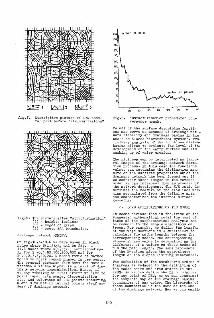
fig.7. Description picture of DEM cent­ral part before "structurizationn

fig.8. The pioture afteJ;' "structurization" (1) - heights isolines (2) - edges of graph ()) - roots FAA boundaries.

drainage network /NMDN/.

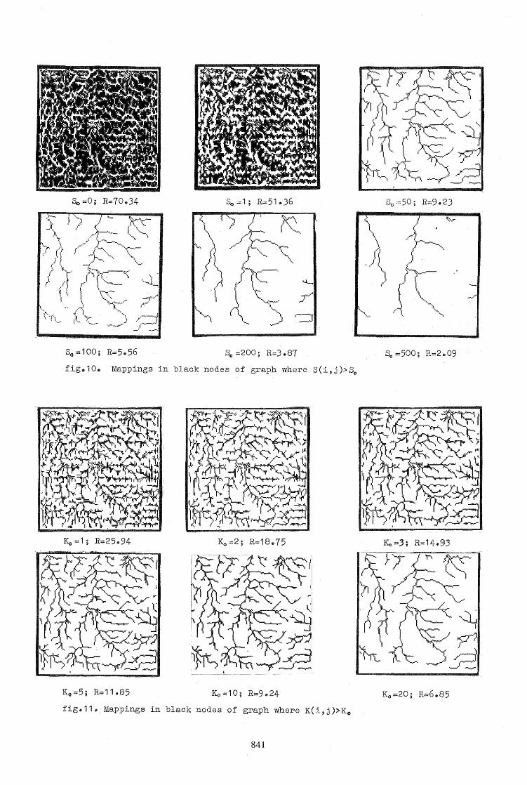
On fig.10.1-10.6 we have shown in black nodes where S(i,j»So and on fig.11.1-11.6 nodes where K(i,j»Ko corresponding­ly for S :0,1,50,100,200,500 and for K =1,2,),5,10,20. R means ratio of marked nodes to their common number in per oents. The present piotures show that the more a threshold is the higher is a level of dra­inage network generalization. Hence, if we say Ifthalveg of first order" we have to point input data scale, discretization step and tolerance of DEM points measurin& K and S values in initial points /leaf no­des/ of drainage network.

840

number of holes

20

20 40 60 so 100 120 -I4Q f60

fig.9. "Structurization prooedure" con-vergence graph.

Values of the surface desoribing funoti­ons may serve as measure of drainage net -work stability and drainage basins in the whole ~s closed hierarchical systems. Pre­liminary analysis of the functions distri­bution allows to evaluate the level of the development of the earth surface and its washing up of water erosion.

The,pictures can be interpreted as tempo­ral images of the drainage network forma­tion prooess. In this case the funotions values can determine the distinction mea­sure of the substrat properties which the drainage network hes been formed on. If we oonsider these images in the reverse order we can interpret them as prooess of the network development. The K/S ratio d~ termines the measure of the flowlines mer­ging aooumulated from the definite area and oharacterizes the internal surface geometry.

4. SOME APPLICATIONS OF THE MODEL

It seems obvious that in the-frame of the suggested mathematioal model the most of tasks of the morphometrical analysis can be reduoed to the Simple algorithms on trees. For example, to define the lengths of thalvegs sections it's suffioient to oaloulate the paths lengths between the oorresponding nodes. The corresponding slopes square value is determined as the difference of S values on these nodes mi­nus the path length. The same prooedure of the K-values gives the approximate length of the slopes limiting watersheds.

The definition of the Strahler's orders ~ thalvegs is reduoed to the definition of the nodes ranks and aros orders in the NMDN. As we oan define the DB boundaries for any point of DEM, so we can construct the oomplete map of the drainage basins boundaries of any order. The hierarchy of these boundaries is the same as the one of the drainage network. Now we can easily

........ ..,j

S(J =200; R=3.87

fig.10. Mappings in black nodes of graph where S(i,j»S"

fig.11., Mappings in black nodes of graph where K(i,j»Ko

841

formulate the procedure of the data pre­paration for the apexes and basic surfa­ces construction.

We have described above the DEM set on the regular grid. The similar description can be used for digital models in the vector presentation, i.e. for the isoli­nes maps processing. In this case we deal with Z-axis ordering data. The construc­tion of the relief sceleton lines frame­work before the raster presentation per­mits to make up the DEM satisfying not only the topographical accuracy but keep.· ing the shape and the structure of the initial surface.

The suggested mathematical model can be considered as the static one. The surface description in the form of the weighted graph permits us to construct a mathema­tical model of the water masses transfe­rence and particle transportation along the surface. If we put infiltration ratio and external water power on nodes and channel capacity on arcs of the graph we can build a mathematical model serving for the flow modeling and erosion proces­ses investigation using simple discrete calculation technique.

REFERENCES

Antipov,M.V., and Kireytov,V.R., 1979. Relief surface T(W) set construction. Ge­ologia i geofizika, 11 :90-97 (in Russian).

Antoshchenko-Olenev,I.V.,and Golda,Ya.V., 1986. Methodology of the automatization of geological interpretation. Sovietskaya geologia, 8:7-15 (in Russian).

Golda, Ya.V., and others, 1986. Working out of methods, algorithms and computer software for automatical construction of geological interpretations map. Report by theme I A.VIII/627 during the period of 1984-1986, Kazgeofizika, Alma-Ata, state register No 26-84-21/31 (in Russian).

Horton,R.E., 1945. Erosional development of streams and their drainage basins: hy­drophysical approach in quantitative mor­phology. Geol. Soc. America Bull., 56:1117-1142.

Kuznetsov,B.M., and others, 1979. The de­vice of inputting of coordinates and heights of stereo terrain model points into ES computer /ItFormat-130 1l / .. In: Aer::i:­al and space automatical data processing methods and technical means. Leningrad, pp.42-55 , (in Russian).

Strahler,A.N .. , 1952. Hypsometric (area­altitude) analysis of erosional topogra­phy. Geol. Soc. America Bull., 62:1117-1142.

Shreve,R.L., 1966. Statistical law of stream numbers. The Journal of Geology, (1):17-37.

842