Embed Size (px)
Citation preview
THE FOOD AID AND FOOD SECURITY ANALYSIS SYSTEM
Jamaica Technical Manual
CARD Technical Report 97-TR 33
Center for Agricultural and Rural Development, Iowa State University, Ames, Iowa
Bureau for Humanitarian Response, United States Agency for International Development
Washington, D.C.
JAMAICA TECHNICAL MANUAL:
CONCEPTUAL FRAMEWORK AND SOFTWARE
DOCUMENTATION
Jacinto Fabiosa, Samarendu Mohanty, Darnell B. Smith,
William H. Meyers, and S. Patricia Batres-Marquez
Center for Agricultural and Rural Development
Iowa State University
Ames, Iowa
Tel: 515-294-1183 · Fax: 515-294-6336
This report was prepared under USAID contract number FAO-0800-C-00-4070-00 with the Center for
Agricultural and Rural Development, Iowa State University.
June 1996

This manual describes the worksheet version of the Food Aid and Food Security Analysis System
(FAFSAS) for Jamaica and details the step-by-step procedure of using this analytical system for policy
analysis.

iii
CONTENTS
FIGURES ..........................................................................................................................................v TABLES ..........................................................................................................................................v CHAPTER 1 - INTRODUCTION......................................................................................................... 1 Scope and Purpose................................................................................................................... 1 How to Use the Manual ........................................................................................................... 2 CHAPTER 2 - CONCEPTUAL FRAMEWORK AND MODEL.............................................................. 3 Key Equations.......................................................................................................................... 4 CARD/FAPRI International Trade Models ..................................................................... 4 The Excess Demand of a Net Importing Country............................................................ 5 The Excess Supply of a Net Exporting Country.............................................................. 5 The Aggregate Excess Supply for M-Country Net Exporters ......................................... 6 The Equilibrium Condition.............................................................................................. 6 Country Commodity Model ............................................................................................. 6 Price Transmission Equations.......................................................................................... 7 Domestic Demand Functions........................................................................................... 7 Domestic Supply Functions ............................................................................................. 8 Net Trade Equation.......................................................................................................... 8 Nutrition Component ....................................................................................................... 9 The Proportion to RDA Equation .................................................................................. 11 Nutrition Component by Socioeconomic and Demographic Population Groups........................................................................... 11 Data, Estimation, and Validation........................................................................................... 12 Data Requirement .......................................................................................................... 12 Parameter Estimation..................................................................................................... 13 Elasticity Estimation ...................................................................................................... 15 Validation Statistics ....................................................................................................... 15
Conclusion ............................................................................................................................. 16
CHAPTER 3 - WORKSHEET DOCUMENTATION ........................................................................... 17
Software and Hardware Requirements .................................................................................. 17 Hard Disk Installation.................................................................................................... 17 The Program File ................................................................................................................... 17
iv
How to Go Through the Program File ................................................................................... 18 BASELINE Worksheet .................................................................................................. 18 SCENARIO Worksheet ................................................................................................. 24 IMPACT Worksheet ...................................................................................................... 24 OUTPUT Worksheet ..................................................................................................... 27 How to Reach the Program Using the Chart ......................................................................... 27 How to Run the Simulation ................................................................................................... 29 CHAPTER 4 - MODIFYING AND UPDATING THE WORKSHEET PROGRAM................................. 31 Availability of New Data....................................................................................................... 31 Reestimation of Equations..................................................................................................... 31 Predicted Values of Exogenous Variables ............................................................................ 31 New Household Expenditure Survey Data ............................................................................ 32 Nutrient Fortification............................................................................................................. 32 Additional Commodity Coverage.......................................................................................... 32 Calibrating the Model to Analyze Specific Policy Questions ............................................... 32 APPENDIX A. DATA REQUIREMENT OF CROP COMPONENT .................................................. 33 APPENDIX B. DATA REQUIREMENT OF LIVESTOCK MEAT COMPONENT............................. 35 APPENDIX C. MACRO DATA REQUIREMENT........................................................................... 37 APPENDIX D. DATA FROM THE HOUSEHOLD EXPENDITURE SURVEY................................... 39 APPENDIX E. THEORETICAL FRAMEWORK OF THE SUPPLY AND DEMAND FUNCTIONS ..... 41 APPENDIX F. PARAMETER ESTIMATES ................................................................................... 43 APPENDIX G. ELASTICITIES...................................................................................................... 61 APPENDIX H. STATISTICS ......................................................................................................... 71 REFERENCES ................................................................................................................................ 75
v
FIGURES 1 Conceptual Framework of the FAFSAS.................................................................................. 4 2 Demand, Supply, and Trade for a Small Open Economy without Trade Distorting Policies.......................................................................................... 10
TABLES 1 Parameter Estimates of Meat Demand .................................................................................. 43 2 Parameter Estimates of Crop Demand................................................................................... 44 3 Parameter Estimates of Corn Feed Demand.......................................................................... 45 4 Parameter Estimates of Soybean Meal Feed Demand........................................................... 45 5 Parameter Estimates of the Number of Cattle Slaughtered ................................................... 46 6 Parameter Estimates of the Average Carcass Weight of Cattle............................................. 46 7 Parameter Estimates of the Number of Pigs Slaughtered...................................................... 47 8 Parameter Estimates of the Average Carcass Weight of Pigs ............................................... 47 9 Parameter Estimates of Chicken Production ......................................................................... 48 10 Parameter Estimates of the Area Planted to Sugar ................................................................ 48 11 Parameter Estimates of the Yield of Sugar............................................................................ 49 12 Parameter Estimates of Wheat Milling.................................................................................. 49 13 Parameter Estimates of the Price Transmission for Wheat .................................................. 50 14 Parameter Estimates of the Price Transmission for Wheat Flour......................................... 51 15 Parameter Estimates of the Price Transmission for Rice ..................................................... 52 16 Parameter Estimates of the Price Transmission for Sugar ................................................... 53 17 Parameter Estimates of the Price Transmission for Corn...................................................... 54 18 Parameter Estimates of the Price Transmission for Cornmeal .............................................. 55 19 Parameter Estimates of the Price Transmission for Soybeans .............................................. 56 20 Parameter Estimates of the Price Transmission for Soybean Meal....................................... 56 21 Parameter Estimates of the Price Transmission for Soy Oil ................................................. 57 22 Parameter Estimates of the Price Transmission for Chicken ................................................ 58 23 Parameter Estimates of the Price Transmission for Beef ...................................................... 59 24 Parameter Estimates of the Price Transmission for Pork ...................................................... 59 25 Marshallian and Expenditure Elasticities for Meat ............................................................... 61 26 Hicksian Elasticities for Meat ............................................................................................... 61 27 Marshallian and Expenditure Elasticities for Crops.............................................................. 61 28 Unconditional Hicksian Elasticities for Crops ...................................................................... 62 29 Differentiated Elasticities in Meat Products by Income and Demographic Groups............................................................................................................. 62 30 Differentiated Elasticities in Crop Products by Income and Demographic Groups............................................................................................................. 65 31 Supply Elasticities for Livestock Meat.................................................................................. 68 32 Supply Elasticities for Sugar Production............................................................................... 69 33 Supply Elasticities for Local Wheat Milling......................................................................... 69 34 Elasticities for the Price Transmission Equation from the World to Border ...................................................................................................... 69 35 Elasticities for the Price Transmission Equation from the Border/Wholesale to Retail..................................................................................... 69
vi
36 Elasticities for the Price Transmission Equation from Border to Wholesale ..................................................................................................... 70 37 Descriptive Statistics of the Model Simulation .................................................................... 71 38 Model Statistics of Fit ........................................................................................................... 72 39 Theil Forecast Statistics......................................................................................................... 73
CHAPTER 1
Introduction
Scope and Purpose
This manual describes the worksheet version of the Food Aid and Food Security Analysis System
(FAFSAS) for Jamaica and details the step-by-step procedure of using the analytical system for policy
analysis. The general purpose of the FAFSAS is to develop a database and analytical system capable of
monitoring and evaluating the impacts of changes in the international markets and in domestic policies
on food security (e.g., food availability and accessibility) of developing countries, especially the food
importing developing countries.
This analytical framework can be used to assess the impacts on domestic food security of changing
global agricultural and trade environments as well as trade policies and domestic market policies in the
country itself. The analysis provided by FAFSAS can be used to evaluate policy decisions within the
country or decisions by donor agencies regarding development assistance or food aid programs. The
information will also enhance interagency coordination of food aid and development resources and
programs, including analytical linkages to nutritional outcomes of significant dietary changes in recipient
countries.
This manual and the accompanying FAFSAS represent a first step in obtaining results by combining
worldwide data from the Food Agricultural Policy Research Institute (FAPRI) models with country-
specific information. The manual provides the basic tools for successfully using and managing the
FAFSAS and includes:
� a conceptual framework and model that combine FAPRI data with country-specific information, described in a series of equations;
� worksheet documentation of the FAFSAS model; � instructions for conducting various policy analyses using this analytical
system.

2 / Fabiosa, Mohanty, Smith, Meyers, and Batres-Marquez
How to Use the Manual
This manual is divided into four chapters. Chapter 1 details the scope and purpose of the manual.
Chapter 2 contains the conceptual framework describing the key equations of the FAFSAS model and
covers production, consumption, net trade, and price transmission. Chapter 3 describes the data sources,
estimation procedures, and parameter estimates, along with elasticities and validation statistics. Chapter
4 documents the worksheet version of this model and also provides step-by-step instructions for running
a simulation. Finally, Chapter 4 includes steps for modifying and updating the worksheet version of the
model.
CHAPTER 2
Conceptual Framework and Model
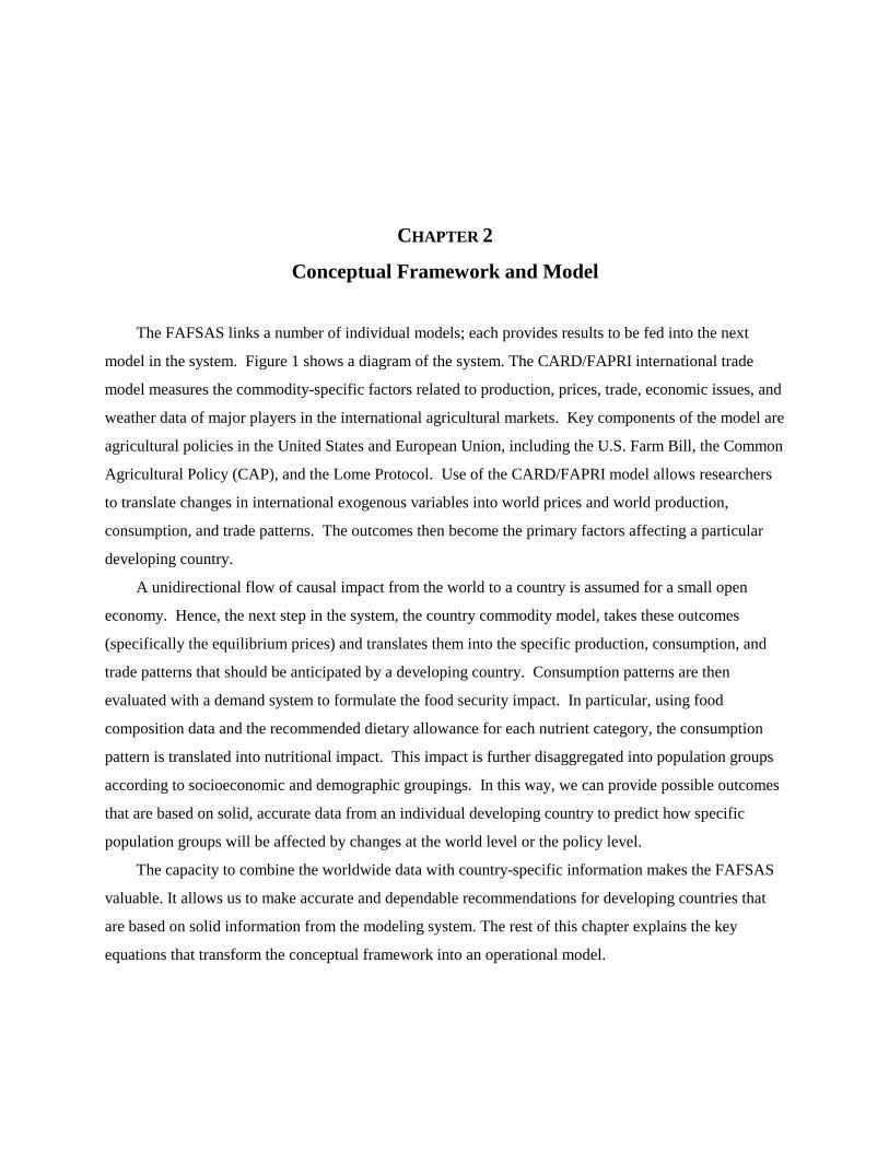
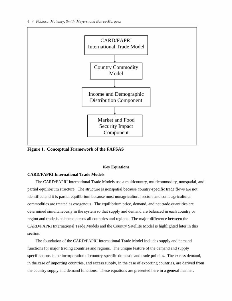
The FAFSAS links a number of individual models; each provides results to be fed into the next
model in the system. Figure 1 shows a diagram of the system. The CARD/FAPRI international trade
model measures the commodity-specific factors related to production, prices, trade, economic issues, and
weather data of major players in the international agricultural markets. Key components of the model are
agricultural policies in the United States and European Union, including the U.S. Farm Bill, the Common
Agricultural Policy (CAP), and the Lome Protocol. Use of the CARD/FAPRI model allows researchers
to translate changes in international exogenous variables into world prices and world production,
consumption, and trade patterns. The outcomes then become the primary factors affecting a particular
developing country.
A unidirectional flow of causal impact from the world to a country is assumed for a small open
economy. Hence, the next step in the system, the country commodity model, takes these outcomes
(specifically the equilibrium prices) and translates them into the specific production, consumption, and
trade patterns that should be anticipated by a developing country. Consumption patterns are then
evaluated with a demand system to formulate the food security impact. In particular, using food
composition data and the recommended dietary allowance for each nutrient category, the consumption
pattern is translated into nutritional impact. This impact is further disaggregated into population groups
according to socioeconomic and demographic groupings. In this way, we can provide possible outcomes
that are based on solid, accurate data from an individual developing country to predict how specific
population groups will be affected by changes at the world level or the policy level.
The capacity to combine the worldwide data with country-specific information makes the FAFSAS
valuable. It allows us to make accurate and dependable recommendations for developing countries that
are based on solid information from the modeling system. The rest of this chapter explains the key
equations that transform the conceptual framework into an operational model.
4 / Fabiosa, Mohanty, Smith, Meyers, and Batres-Marquez
CARD/FAPRI International Trade Model
Country Commodity Model
Income and Demographic Distribution Component
Market and Food Security Impact
Component
Figure 1. Conceptual Framework of the FAFSAS
Key Equations
CARD/FAPRI International Trade Models
The CARD/FAPRI International Trade Models use a multicountry, multicommodity, nonspatial, and
partial equilibrium structure. The structure is nonspatial because country-specific trade flows are not
identified and it is partial equilibrium because most nonagricultural sectors and some agricultural
commodities are treated as exogenous. The equilibrium price, demand, and net trade quantities are
determined simultaneously in the system so that supply and demand are balanced in each country or
region and trade is balanced across all countries and regions. The major difference between the
CARD/FAPRI International Trade Models and the Country Satellite Model is highlighted later in this
section.
The foundation of the CARD/FAPRI International Trade Model includes supply and demand
functions for major trading countries and regions. The unique feature of the demand and supply
specifications is the incorporation of country-specific domestic and trade policies. The excess demand,
in the case of importing countries, and excess supply, in the case of exporting countries, are derived from
the country supply and demand functions. These equations are presented here in a general manner.
Jamaica Technical Manual: Conceptual Framework and Software / 5
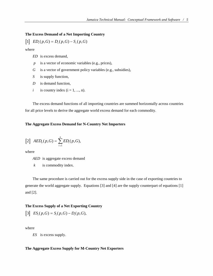
The Excess Demand of a Net Importing Country
� �1 ED p G D p G S p Gi i i( , ) ( , ) ( , )� �
where
ED is excess demand,
p is a vector of economic variables (e.g., prices),
G is a vector of government policy variables (e.g., subsidies),
S is supply function,
D is demand function,
i is country index (i = 1, ..., n).
The excess demand functions of all importing countries are summed horizontally across countries
for all price levels to derive the aggregate world excess demand for each commodity.
The Aggregate Excess Demand for N-Country Net Importers
� �2 AED p G ED p Gk ii
n
( , ) ( , ),��
�1
where
AED is aggregate excess demand
k is commodity index.
The same procedure is carried out for the excess supply side in the case of exporting countries to
generate the world aggregate supply. Equations [3] and [4] are the supply counterpart of equations [1]
and [2].
The Excess Supply of a Net Exporting Country
� �3 ES p G S p G D p Gi i i( , ) ( , ) ( , ),� �
where
ES is excess supply.
The Aggregate Excess Supply for M-Country Net Exporters
6 / Fabiosa, Mohanty, Smith, Meyers, and Batres-Marquez
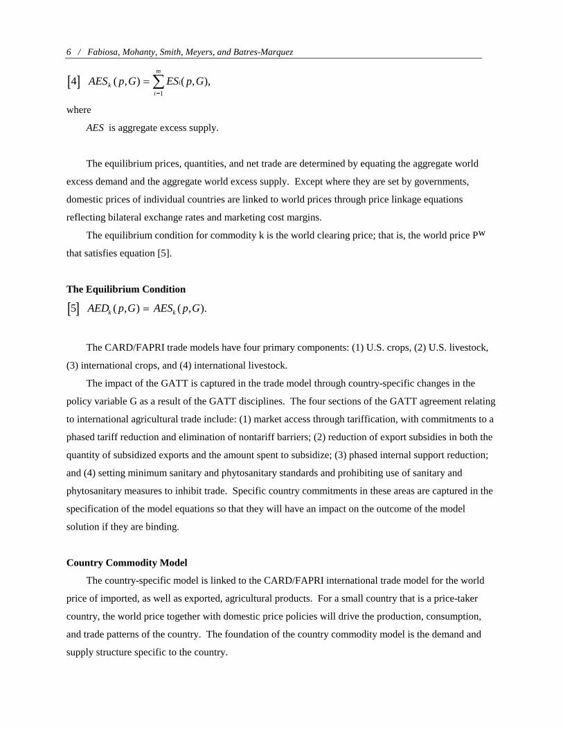
� �4 AES p G ES p Gk i
i
m
( , ) ( , ),��
�1
where
AES is aggregate excess supply.
The equilibrium prices, quantities, and net trade are determined by equating the aggregate world
excess demand and the aggregate world excess supply. Except where they are set by governments,
domestic prices of individual countries are linked to world prices through price linkage equations
reflecting bilateral exchange rates and marketing cost margins.
The equilibrium condition for commodity k is the world clearing price; that is, the world price Pw
that satisfies equation [5].
The Equilibrium Condition
� �5 AED p G AES p Gk k( , ) ( , ).�
The CARD/FAPRI trade models have four primary components: (1) U.S. crops, (2) U.S. livestock,
(3) international crops, and (4) international livestock.
The impact of the GATT is captured in the trade model through country-specific changes in the
policy variable G as a result of the GATT disciplines. The four sections of the GATT agreement relating
to international agricultural trade include: (1) market access through tariffication, with commitments to a
phased tariff reduction and elimination of nontariff barriers; (2) reduction of export subsidies in both the
quantity of subsidized exports and the amount spent to subsidize; (3) phased internal support reduction;
and (4) setting minimum sanitary and phytosanitary standards and prohibiting use of sanitary and
phytosanitary measures to inhibit trade. Specific country commitments in these areas are captured in the
specification of the model equations so that they will have an impact on the outcome of the model
solution if they are binding.
Country Commodity Model
The country-specific model is linked to the CARD/FAPRI international trade model for the world
price of imported, as well as exported, agricultural products. For a small country that is a price-taker
country, the world price together with domestic price policies will drive the production, consumption,
and trade patterns of the country. The foundation of the country commodity model is the demand and
supply structure specific to the country.
Jamaica Technical Manual: Conceptual Framework and Software / 7
Price Transmission Equations
Price transmission equations provide the bridge between the world price and a country’s internal
price. The new set of world prices determined in the CARD/FAPRI trade model is transmitted to the
Jamaican country commodities model through these price transmission equations. Ideally, the border
price in Jamaica differs from the world price by the transportation cost. Since the world price and border
price are highly correlated, it is adequate to generate the border price as a function of the world price.
For the kth commodity, this is
[6] P f P ER Ckb
kw
k = ( , , ) ,
where
P is the border price for the kth commodity,
Pw is the world price for the kth commodity,
ER is exchange rate,
C is marketing cost,
k is the index for commodity.
All domestic prices are expressed in the local currency and the world price is in U.S. dollars. ER is
the price of one U.S. dollar in local currency (i.e., the exchange rate). Marketing cost is represented by
the variable C, which may include markup, transportation, labor, and other marketing costs. Whenever
appropriate, the consumer price index is used as a proxy of marketing cost for the price transmission
between different levels in the market chain. Also, possible lags and inclusion of other variables in the
regression equations will be determined empirically.
Domestic Demand Functions
The aggregate demand includes demand for human consumption, feed use, inventory demand, and
demand for industrial use. The dominant component of aggregate demand includes both human and feed
use. The quantity demanded for human consumption is expressed as a function of own-price, prices of
related commodities (e.g. substitutes and compliments), consumption expenditures, and other shifters
(e.g. to account for dynamics and time trend).
� �7 Q f p P X Zkd
k s d d� ‘( , , , | )� ,
8 / Fabiosa, Mohanty, Smith, Meyers, and Batres-Marquez
where
Q is the quantity demanded,
p is the own price,
P is a vector of prices of related commodities,
X is real expenditure/income,
Z is a vector of other shifters in the demand equation,
� is a vector of demand coefficients,
d superscript and subscript for demand.
Feed demand is a derived demand that is a function of feed price and the livestock price as the major
output.
Domestic Supply Functions
The quantity supplied, on the other hand, is expressed as a function of own price, price of inputs,
and other shifters:
� �8 Q f p W Zks
k s s� ‘( , , | ),�
where
Q is quantity supplied,
W is a vector of input prices,
Z is a vector of other shifters in the supply equation,
� is a vector of supply coefficients,
s superscript and subscript for supply.
The equilibrium condition is given in equation [9], where the net quantity traded (quantity imported or
exported) is equal to the difference between the domestic quantity demanded and supplied at the
equilibrium price.
Net Trade Equation
� �9 Q Q Qknt
ks
kd� � ,
Jamaica Technical Manual: Conceptual Framework and Software / 9
where
Q is net trade (export if positive and import if negative),
nt superscript for net trade.
For a small open economy, the equilibrium is determined by its domestic demand and supply
structure and by international market conditions. If the domestic equilibrium price under autarchy is
below the world price, the country is a net exporter of that commodity. On the other hand, if the
domestic equilibrium price under autarchy is above the world price, the country is a net importer. In the
absence of trade distorting policies, a country has an excess demand (in case of net importers) or an
excess supply (in case of net exporters). The country faces a perfectly elastic import supply (for net
importers) or export demand (for net exporters) since it cannot influence the world market. In this case,
world market prices are fully transmitted to the domestic market. Any price differential between
domestic and world prices is fully attributed to transport cost. Figure 2 illustrates the case of a small
open economy in the absence of trade distorting policies.
Nutrition Component
The new set of Jamaican prices enter the Jamaican commodity model through the estimated supply
and demand equations of the respective commodities (i.e., equations [7], [8], and [9]). The outcomes of
the commodity model are per capita consumption patterns of households, production, and trade patterns.
The per capita consumption levels of households by commodities will serve as the input in the nutrition
component to determine the macro- and micronutrient intake levels. The consumption of products is
translated into nutrient intake using
� �10 TN Ql lk kd
k
n
��
�� . ,1
where
TN is total nutrient intake,
� is the proportion of nutrient per unit weight of commodity consumed,
l is the index for nutrient,
where TN is the total nutrient intake of the lth nutrient, and �lk is the proportion of the lth nutrient (e.g.,
energy) per unit (e.g., lb) of the kth commodity consumed (e.g., wheat). The vector of n-products (Q with
index k) consumed includes wheat, rice, sugar, soy oil, cornmeal, poultry, beef, and pork. The
10 / Fabiosa, Mohanty, Smith, Meyers, and Batres-Marquez
ED = D - S
ES = S - D
Pa
Pw
S
D
i) Net Importer Case
Pa
Pw
S
D
ii) Net Exporter Case
Q s Q d
Qm
Qm
Q d Q s
Q e
Q e
Figure 2. Demand, Supply, and Trade for a Small Open Economy without Trade Distorting Policies
Notes: Pa = autarchy price, Pw = world price.
vector of macro- and micronutrients (the index l) includes energy, protein, fat, carbohydrates, fiber,
calcium, iron, vitamin A, thiamine, riboflavin, and niacin.
Furthermore, to evaluate the nutritional outcomes of policy changes, the nutrient intake levels are
compared with their respective recommended dietary allowances (RDAs) to determine the degree of
shortfall (or excess) from the RDAs. To be comparable to the RDA standard, the nutrient intake has to
Jamaica Technical Manual: Conceptual Framework and Software / 11
be expressed on a per day basis. A measure of nutrition adequacy is the ratio of the total intake of
nutrient l to its corresponding recommended dietary allowance.
The Proportion to RDA Equation
� �11 ADQTN
RDAll
l
�,
where
ADQ is a measure of nutrient adequacy,
RDA is recommended dietary allowance.
If this ratio in [11] approaches unity, it implies that the intake of the lth nutrient is adequate in meeting the
recommended dietary allowance for that particular nutrient.
Nutrition Component by Socioeconomic and Demographic Population Groups
Different population groups (grouped by socioeconomic and demographic characteristics) are
affected differently by changes in the economy (i.e., price changes). Of significant interest is population
grouping by income. Other than possible differences in taste and preference between low- and high-
income groups, their responses to price changes will also differ due to different proportions of
expenditure for the commodities in their food basket and different income elasticities. The nutritional
impact on households disaggregated further into socioeconomic and demographic characteristics is
examined. The nutrition measures in [10] and [11] are reproduced for each of the population groups by
socioeconomic and demographic characteristics. That is, the total nutrient intake is:
� �12 TN Qlh
lk kd h
k
n
��
�� . ,
1
where
h is index of household socioeconomic and demographic groupings and the ratio of total nutrient
intake to RDAs is:
� �13 ADQTN
RDAlh l
h
l
� .
The added index h represent the hth household group based on socioeconomic and demographic
characteristics. The key groupings are based on income. Different price and income elasticities are
12 / Fabiosa, Mohanty, Smith, Meyers, and Batres-Marquez
derived for each income group. Differential price and income elasticities of households in different
income groups drive the differences in the consumption and nutritional impacts.
Consumption and nutrition impact are also analyzed for household groupings based on geographical
location, family size, and head of household characteristics such as age, gender, and occupation.
Data, Estimation, and Validation
Data Requirement
The data requirements of the model are listed in Appendices A to D. Time series data for a number
of variables were needed to estimate the model and generate reasonable demand and supply estimates.
The consumption time series was approximated by the disappearance series. The disappearance series is
derived as a residual in an accounting identity of the sources and uses of a commodity. Sources of a
commodity include current production, imports, and beginning inventory. The uses of a commodity
(excluding human consumption) are feed use, industrial use, exports, and ending inventory. Human
consumption is calculated by deducting nonfood uses from sources of supply. This approach was used
for meat and crops.
Data needed for crop supply were area planted and harvested, total production, yield, and other
factors affecting supply such as weather data. Data for meat supply included animal inventory, number
slaughtered, and average weight.
Price data for all commodities in the model at all levels in the marketing chain were also needed.
These included world price, border price, wholesale price, and retail price. Farm price was also recorded
when available. Prices of related commodities (i.e., complements and substitutes) and prices of inputs
such as fertilizer and feeds were also collected. Basic macroeconomic data such as population, gross
domestic product, exchange rate, and consumer price index were also needed. Policy variables included,
in particular, the schedule of external and internal tariffs, producer support, and consumer support.
Appendices A, B, and C list the basic data requirements.
Data from the Household Expenditure Survey were needed to examine differences in the
expenditure, consumption, and nutrient intake of households at different income levels and in other
sociodemographic groups. These data are listed in Appendix D.
The Jamaican data were collected from a number of sources. Most of the domestic production data
came from the Economic and Social Survey of Jamaica (various years), an annual publication prepared
by the Planning Institute of Jamaica. Production Statistics (various years) of the Statistical Institute of
Jamaica also provided production data and wholesale values for some major commodities. Data in this
publication came from Commodity Boards and Associations, Agricultural Planning Agencies, the
Jamaica Technical Manual: Conceptual Framework and Software / 13
Ministry of Agriculture, and direct returns from producers—large manufacturing enterprises. Production
statistics for processed agricultural products came from the Statistical Digest published by the Research
and Programming Division of the Bank of Jamaica. The trade data were collected from External Trade
(various years) Parts I and II, Statistical Institute of Jamaica. The raw information summarized in the
trade data was collected from declarations of importers and exporters presented to the commissioner of
customs and excise, as mandated under the Customs and Exchange Control Act. The retail price data
were published in the Consumer Price Index, Statistical Institute of Jamaica. World prices were
collected from International Financial Statistics and the USDA Situation and Outlook Reports for various
commodities. The Statistical Yearbook of Jamaica, Statistical Institute of Jamaica, was the main source
for most of the macro variables.
Other unpublished information was collected from personal visits to various agencies of the
Government of Jamaica, including the Ministry of Agriculture, Ministry of Welfare and Labor, Ministry
of Finance, and the Bank of Jamaica.
Parameter Estimation
The data cover 1972 to 1993. Since Jamaica is a small importer of most commodities,1 it faces a
perfectly elastic import supply, making the price exogenous as determined by the world market. Border
duties and internal taxes simply put a wedge between the world price and domestic price. The demand
and supply functions can thus be estimated separately without introducing simultaneity bias in the
estimates. The supply equations for commodities with local production were estimated using ordinary
least squares (OLS). The demand side of the structural model was treated as a separate block and
estimated as a system of equations using Iterative Three-Stage Least Squares. This method gives
Maximum Likelihood Estimates at the point of convergence.
Crop and meat demand are specified as an Almost Ideal Demand System (AIDS) specification
because of the system’s desirable properties. It has a flexible, functional form since it is derived from a
second-order approximation of the cost function. When the Stone Price Index is used, the final
estimating equation is linear in parameters. Also, it makes it easy to impose demand theoretical
properties (i.e., adding-up, homogeneity, and symmetry) through cross-equation parametric restrictions.
Furthermore, the systems estimation exploits information from the covariance matrix that improves
1 This is not the case for the beef and pork supply. However, the production lags in beef and pork lessen
the simultaneity.
14 / Fabiosa, Mohanty, Smith, Meyers, and Batres-Marquez
efficiency of estimates (i.e., SURE-type advantage). Actual estimation was accomplished through SAS
and RATS version 4.0.
The standard specification of an AIDS model expresses the expenditure share of each commodity as
a function of its own price, prices of related commodities (complements and substitutes), and real
expenditure. In our specification, lag values of the expenditure share, lag values of some independent
variables, and trend were included to capture dynamic adjustments of consumers. Moreover, the model
is reformulated to allow direct estimation of the long-run parameters. The theoretical demand properties
were imposed only on the long-run parameters. The estimated parameters for demand systems (crops and
livestock), supply systems, and price transmission equations are presented in Appendix F(Tables 1 to 24).
Elasticities estimated from these parameters, including differentiated elasticities in crops and meat
products by income and demographic groups, are also presented in Appendix G (Tables 25 to 36).
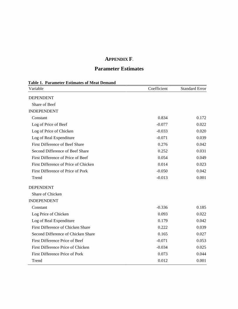
Table 1 shows the estimates of the meat demand and Table 2 the crop demand estimates. The
adequacy of the estimated model is reflected by a number of statistics. The estimated model displays all
the theoretical demand properties since these were imposed in the estimation. The long-run parameter
estimates have correct signs as shown in the elasticities derived from them. That is, own-price
elasticities are negative and expenditure elasticities are all positive. Many of the long-run parameters
have coefficient estimates that are significant. Also, lagged regressors and trend are significant,
suggesting dynamic adjustment of consumers. Table 3 gives estimates of the feed demand for corn and
Table 4 gives estimates of the feed demand for soybean meal.
Tables 5 to 9 present estimates of the supply equations of beef, pork, and poultry. Tables 10 to 12
give estimates of the supplies of sugar and milled wheat. The supply functions show very good fit with
R2, mostly in the high 80 and 90 percent range. Durbin-Watson statistics suggest the absence of strong
serial correlation.2 A joint test for absence of serial correlation with order higher than one using the
Ljung-Box Q(r)-statistic accepts the hypothesis that the first r autocorrelation is random with a true value
of zero.3 Parameter estimates are theoretically consistent, giving the expected positive sign for own price
and the negative sign for the input price in a standard supply function. Collinearity may be present,
especially when the R2 is high but individual regressors have low t-values. This can be remedied in a
number of ways, such as the principal components method. But since the model is primarily for
2 Some of the D-W statistics are in the inconclusive range. The D-W is not a formal test when lagged
values of the dependent variable are in the set of regressors. 3 Values of the Q(r)-statistics are not reported in the tables.
Jamaica Technical Manual: Conceptual Framework and Software / 15
simulation purposes, this was not pursued. When collinearity is present, estimates are still unbiased but
not very efficient.
Tables 13 to 24 give the estimates of the price transmission equations. Linear and logarithmic
functions were used according to what was statistically appropriate. The price transmission equations
show very good fit with R2 , mostly in the high 90 percent range. Most of the Durbin-Watson statistics
suggest the absence of serial correlation. The absence of serial correlation is also corroborated by the
joint test using the Ljung-Box Q(r)-statistic. Parameter estimates are consistent with the expected
direction of impact of price change transmission in the market chain. That is, an increase in the world
price would increase the price at the border, wholesale, and retail levels. Also, changes in the exchange
rate (i.e., devaluation) increase the domestic price.
Elasticity Estimation
Elasticity estimates provide a scale-free measure of demand or supply responsiveness to changes in
its arguments (i.e., own price, income, and input price). The sign of elasticity checks whether the
minimum requirement of a downward sloping demand and upward sloping supply are met. Tables 25 to
28 give the demand elasticity estimated from the time series. The own-price elasticities are all negative
and all the expenditure elasticities are positive. Moreover, the absolute values of the elasticities are
within the range reported for these commodities in other studies. Also, differentiated elasticities by
population groups were estimated by merging the time series elasticity with disaggregated information
from the Household Expenditure Survey. These estimates are given in Tables 29 and 30.
The supply elasticities are shown in Tables 31 to 33. The meat and crop supply elasticities show a
positive own-price elasticity and negative input price elasticities. Feed is the major input in meat
production and fertilizer in crop production. The price transmission elasticities show a positive price
transmission from the world to the border, from the border to wholesale, and from wholesale to retail
level (Tables 34 to 36). Prices at the border respond positively to devaluation of local currency. Prices
at the wholesale and/or retail level respond positively to increases in the consumer price index, which is
used as a proxy of marketing cost.
Validation Statistics
Historical simulation of the model’s core equation was employed to validate the estimated model
with a selected set of validation statistics. These statistics are presented in Appendix H (Tables 37 to
39). Table 37 shows the mean of actual and predicted values for the core endogenous variables; the mean
of the predicted values are very close to the mean of the actual values, suggesting that the model is
16 / Fabiosa, Mohanty, Smith, Meyers, and Batres-Marquez
adequate. Table 38 shows the prediction error expressed relative to the actual values of the endogenous
variables. The first column is the mean of the error. The second column reports the mean of the absolute
value of the prediction error. The third column is the root of the mean square error. All three statistics
are expressed as a percentage of the actual values of the endogenous variables. Smaller values indicate a
good model.
Table 39 decomposes the Mean Square Error (MSE) into three components: bias, variance, and
covariance. The second decomposition includes the bias, regression, and disturbance. The latter offers
more intuitive appeal than the former. The bias and regression components capture the systematic
divergence of the prediction from actual values. Hence, for a good model, the proportion of bias and
regression should approach a small number. On the other hand, the disturbance component, which
accounts for the random divergence of the prediction from the actual values, should explain a large
proportion of the MSE. Its value should approach one..4
Conclusion
The data requirements of the model were collected from various sources such as international
organizations and local agencies in Jamaica. Estimation was done in SAS and RATS. Standard
diagnostics and validation statistics suggest the model’s adequacy in capturing changes in the historical
data.
4 In the first decomposition, a good model will have the covariance component approaching one.
CHAPTER 3
Worksheet Documentation
The conceptual framework and estimated parameters, along with elasticities, have been described in
previous chapters. This chapter provides detailed information on the installation requirements and use of
the worksheet version of the FAFSAS. The discussion assumes that the user is familiar with the basic
concepts and operation of DOS and Lotus 123.
Software and Hardware Requirements
The worksheet version of the FAFSAS is in Lotus Release 4 or 5. The requirements to run the
FAFSAS model include Windows 3.1 or later version, DOS 3.30 or later version, and Lotus 123 Release
4 or 5.
The hardware requirements are 386 or later model PC, mouse, 24 MB RAM (preferably more), 13.7
Mg Program File, and VGA or better monitor.
Hard Disk Installation
It is recommended that the program file “FAFSAS.WK4” be placed in a separate directory. If a
suitable directory does not exist, create one using the DOS MD or MKDIR command. Make certain the
DOS prompt is in the root directory of the hard disk (C:). Type: C:>MD \ <directory name> {Enter}.
Choose a directory name of not more than eight characters; we recommend FAFSAS for the name of
the directory on the installation command line. After creating a suitable directory, copy the program file
into the FAFSAS directory by typing the following:
C:\COPY <drive:\FAFSAS.WK4>
The Program File
The program file (FAFSAS.WK4) accommodates future policy simulation questions. In particular,
this program file is designed to examine the impact of changes in international trade agreements such as
the GATT, and changes in domestic border policies such as the duty and tax structure.

18 / Fabiosa, Mohanty, Smith, Meyers, and Batres-Marquez
The program file contains four worksheets. The first is the PARAMETER worksheet in which the
user specifies the parameters of the policy simulation analysis. The second is the BASELINE worksheet
that includes the data that are used in the baseline and the equations that generate the relevant
endogenous variables using the baseline data. Third is the SCENARIO worksheet. It is very similar to
the baseline worksheet in terms of its equation structure. The only difference is that the data values in
this worksheet will reflect policy analysis as specified in the parameter worksheet. Last is the IMPACT
worksheet, which is composed of three sections. The IMPACT 1 sheet contains change of consumption,
production, trade, and nutrition for both crops and livestock. It also includes estimates of demand and
nutrition change expressed in percentages, from baseline to scenario for income and demographic groups.
This process is continued in the IMPACT 2 sheet to accommodate all population groups. The
IMPACT 3 sheet contains estimates for both baseline and scenario actual levels of consumption (by
commodity, in pounds) and nutrient intake (by nutrient in kcl, grams, m.grams, and R.E.), by income and
demographic groups. The intake levels are also expressed as proportions of RDA.
The last worksheet, OUTPUT, contains the summary tables for world, border, and retail prices;
production, consumption, and trade of crops and livestock; and consumption and nutrition impact by
quartile, location, gender, age, family size, and occupation. The results are arranged in the form of
baseline, scenario, and percentage changes from baseline to scenario for each variable.
How to Go Through the Program File
When the user loads the program file in Lotus 123, the worksheets in the file will appear in the
“Worksheet Tab,” in the following order: PARAMETER, BASELINE, SCENARIO, IMPACT 1,
IMPACT 2, IMPACT 3, and OUTPUT. To go from one worksheet to another, simply put the mouse
pointer inside the desired worksheet destination and click the left button of the mouse. Once you reach
the desired worksheet, you can move across columns by holding the left button of the mouse at the
appropriate horizontal scroll arrow (left arrow to move left and right arrow to move right), and across
rows by holding the left button of the mouse at the appropriate vertical scroll arrow (top arrow to move
up and button arrow to move down).
BASELINE Worksheet
The key worksheet in the program file is the baseline worksheet that shows the economic structure
of the model. The baseline worksheet is divided into two subsections: the data section and the equation
section.
Jamaica Technical Manual: Conceptual Framework and Software / 19
Data Section
The data requirements of the model were discussed in the previous chapter. Among other things, these
include price, macroeconomic, consumption, production, import, inventory, feed use, industrial use, and
export data.
Also, data from the Household Expenditure Survey were needed to examine differences in the
expenditure, consumption, and nutrient intake of households at different income levels in other
socioeconomic and demographic groups.
A sample of the data section is presented here. Column A gives the row address of the data series
(e.g., number of cattle slaughtered is in row 134). Column B gives the mnemonic names corresponding
to each of the data series (e.g., CAKTNJA_ is the name given to the variable number of cattle
slaughtered).5 Column C provides the descriptive name of the data series. Column D is the unit of
measure (e.g., Head). Column E gives the source of the data (e.g., JSES is the Jamaica Economic and
Social Survey). The actual data begin in Column K for 1972, the start of the series, and extend up to
column AF for 1993.
A B C D E
DATA
130 UNITS SOURCE 131 YEAR 132 133 CATTLE PRODUCTION DATA 134 CAKTNJA_ Number of Cattle Slaughtered Head JSES 135 CAKTDJA_ Total Beef Production 000 Lbs JSES 136 CAKADJA_ Average Carcass Weight Cattle LBS/Head JSES
Equation Section
To maintain tractability, this model is solved recursively. That is, the CARD/FAPRI International
Trade Model is solved first, then the solution values of the endogenous variables (e.g., world equilibrium
prices) are inputted as given data in the solution of the country commodity model. This greatly reduces
the model’s complexity.
5 The first two letters refer to the commodity (e.g., CA for cattle), the next three letters refer to the
activity (e.g., KTN for number slaughtered), and the last two letters refer to the country (e.g., JA for Jamaica). Mnemonic names are included in the worksheet because they allow easy cross-referencing using the @vlookup function in Lotus 123.
20 / Fabiosa, Mohanty, Smith, Meyers, and Batres-Marquez
The equation section gives the worksheet address of the equation, the dependent variable, the list
of independent variables, estimated coefficients, and the worksheet formula and function that translate
the functional form and algebraic relations of the model’s equations into worksheet equations.
Coefficient Estimates
The key elements of the equation section are the coefficient estimates. The performance of the
entire model rests largely on whether the coefficient estimates are theoretically consistent and
statistically acceptable. The coefficient estimates were given in the previous section.
Nutrient Coefficient and RDAs
The nutrient coefficient, which measures the amount of a particular nutrient available from a unit of
commodity consumed, is needed to convert consumption of commodities into nutrient intake. This
information is taken from Food Composition Tables.6 To assess the adequacy (or inadequacy) of the
nutrient intake for population groups, their level of nutrient intake is compared to the Recommended
Dietary Allowance. The RDAs are intended as benchmark numbers that indicate fulfillment of the
nutritional needs in ordinary life situations. An adequate nutrient intake level is in the neighborhood of
the RDAs.
Model Component Description
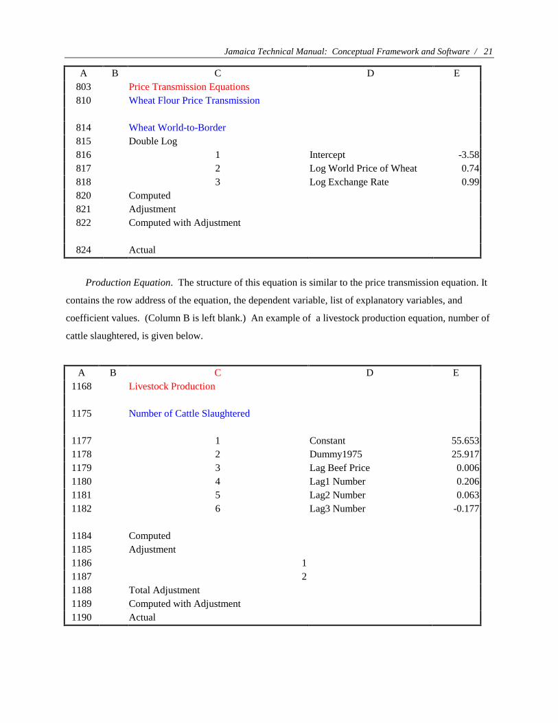
Price Transmission Equation. Column A gives the row address of this equation (i.e., row 1).
Column C gives the descriptive name of the equation and the endogenous variables. Column D lists all
the explanatory variables that include an intercept, log of world price of wheat, and log of exchange rate.
Column E gives the coefficient values corresponding to each of the explanatory variables, which in this
example are -3.58, 0.74, and 0.99, respectively. Disaggregating the equation into separate rows for each
of the explanatory variables has the added advantage of allowing a more detailed examination of which
specific variables are significantly affecting the endogenous variable. The computed and actual values
are included for comparison purposes. An example of wheat price transmission from world to border is
provided below.
6 The nutrient coefficient for Jamaica is taken from the “Food Composition Tables—For Use in the
English-Speaking Caribbean,” compiled by the Caribbean Food and Nutrition Institute, Kingston, Jamaica.
Jamaica Technical Manual: Conceptual Framework and Software / 21
A B C D E 803 Price Transmission Equations 810 Wheat Flour Price Transmission
814 Wheat World-to-Border 815 Double Log 816 1 Intercept -3.58 817 2 Log World Price of Wheat 0.74 818 3 Log Exchange Rate 0.99 820 Computed 821 Adjustment 822 Computed with Adjustment
824 Actual
Production Equation. The structure of this equation is similar to the price transmission equation. It
contains the row address of the equation, the dependent variable, list of explanatory variables, and
coefficient values. (Column B is left blank.) An example of a livestock production equation, number of
cattle slaughtered, is given below.
A B C D E 1168 Livestock Production
1175 Number of Cattle Slaughtered
1177 1 Constant 55.653 1178 2 Dummy1975 25.917 1179 3 Lag Beef Price 0.006 1180 4 Lag1 Number 0.206 1181 5 Lag2 Number 0.063 1182 6 Lag3 Number -0.177
1184 Computed 1185 Adjustment 1186 1 1187 2 1188 Total Adjustment 1189 Computed with Adjustment 1190 Actual
22 / Fabiosa, Mohanty, Smith, Meyers, and Batres-Marquez
Meat Trade Equation. Net trade is the difference between production and consumption. Since net
trade is an accounting equation, there are no estimated parameters.
A B C D 1385 Meat Trade
1389 Beef Trade
1391 BEP_JA_b Beef Production 1392 Beef Production 1393 Beef Consumption 1394 Beef Imports Consumption - Production 1395 Beef Imports with Adjustments Consumption - Production 1396 BEI_JA_b Beef Imports with Adjustments
Nutrient Intake Equation. The consumption values are translated into nutrient intake (e.g., energy)
using the appropriate food composition data. Column C contains all the commodities in the household
food basket. Column E gives the coefficient that measures the amount of nutrient (e.g., energy) derived
from the consumption of a unit (e.g., one lb) of a commodity (e.g., beef). The sum of nutrient intake over
all commodities consumed gives the total nutrient intake. Since this total nutrient intake is compared
with the RDA values for each nutrient, it is expressed on a per day nutrient intake basis.
A B C D E 1801 Average Nutrient Intake
1804 Energy Intake 1805 BEENPJA_b Beef ENBF 1016 1806 HPENPJA_b Pork ENPK 980 1807 CKENPJA_b Chicken ENCK 815 1808 WHENPJA_b Wheat Flour ENWT 1674 1809 REINPJA_b Rice ENRC 1647 1810 SUENPJA_b Sugar ENSG 1692 1811 SOENPJA_b Soy oil ENSO 3850 1812 CMENPJA_b Cornmeal ENML 1651 1813 ENPJA_b Total Per Capita Daily Intake Energy
Proportion of RDAs Equation. The nutrient intake is compared to the recommended dietary
allowance to evaluate the nutritional adequacy of the consumption of households. The recommended
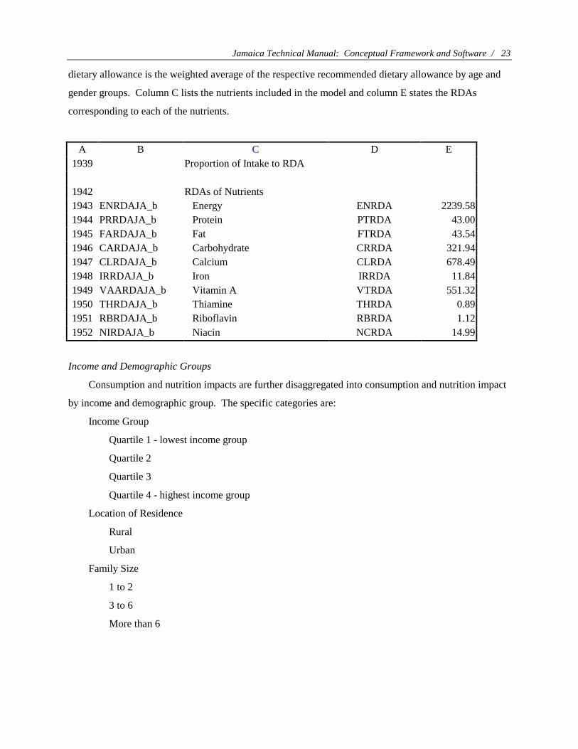
Jamaica Technical Manual: Conceptual Framework and Software / 23
dietary allowance is the weighted average of the respective recommended dietary allowance by age and
gender groups. Column C lists the nutrients included in the model and column E states the RDAs
corresponding to each of the nutrients.
A B C D E 1939 Proportion of Intake to RDA
1942 RDAs of Nutrients 1943 ENRDAJA_b Energy ENRDA 2239.58 1944 PRRDAJA_b Protein PTRDA 43.00 1945 FARDAJA_b Fat FTRDA 43.54 1946 CARDAJA_b Carbohydrate CRRDA 321.94 1947 CLRDAJA_b Calcium CLRDA 678.49 1948 IRRDAJA_b Iron IRRDA 11.84 1949 VAARDAJA_b Vitamin A VTRDA 551.32 1950 THRDAJA_b Thiamine THRDA 0.89 1951 RBRDAJA_b Riboflavin RBRDA 1.12 1952 NIRDAJA_b Niacin NCRDA 14.99
Income and Demographic Groups
Consumption and nutrition impacts are further disaggregated into consumption and nutrition impact
by income and demographic group. The specific categories are:
Income Group
Quartile 1 - lowest income group
Quartile 2
Quartile 3
Quartile 4 - highest income group
Location of Residence
Rural
Urban
Family Size
1 to 2
3 to 6
More than 6
24 / Fabiosa, Mohanty, Smith, Meyers, and Batres-Marquez
Gender of Head of Household
Male
Female
Age of Head of Household
Less than 25
25 to 65
More than 65
Occupation of Head of Household
Professional
Self-employed Agriculture
Self-employed Nonagriculture
Services
Others.
SCENARIO Worksheet
The simulation worksheet is structured much like the BASELINE worksheet. That is, the first
section contains the data set and the succeeding rows contain the equations. The main difference is in the
data section. Some of the data in the scenario worksheet are conditioned on the specification of the
policy simulation analysis entered in the parameter worksheet. The changes in these data will drive the
changes in the values of endogenous variables. For example, retail prices in the scenario data section
will change if food aid supply is reduced. The degree of price change depends on the amount of food aid
reduction and flexibility assumption.
IMPACT Worksheet
The outputs of the policy simulation analysis are contained in the IMPACT Worksheet. The outputs
are presented in terms of the average or representative household/person and in terms of the
socioeconomic and demographic groupings. The demographic characteristics include income, which is
divided into four quartiles; age, with three categories; location - urban or rural; family size, with three
categories; gender of head of household - male or female; and occupation of head of household, with five
categories (e.g., self-employed agriculture).
Jamaica Technical Manual: Conceptual Framework and Software / 25
At the mean level, impact outputs include the baseline and scenario values of production,
consumption, and net trade for all commodities in the model; nutrient intake; and proportions of the
nutrient intake relative to their corresponding RDAs. For the socioeconomic and demographic groups,
the impact output is in terms of levels and percentage changes in consumption by commodity, nutrient
intake, and proportions to RDAs.
The demand equations for different income and demographic groups are expressed in elasticity
form. This is necessary since the additional theoretical property, that is the Slutsky decomposition used
to adjust the average elasticity into income and demographic groups, is easily accomplished in elasticity
form. Adjusting the average elasticity is the best approach since direct estimation by income and
demographic groups is impossible with the limited data from household expenditure surveys. The
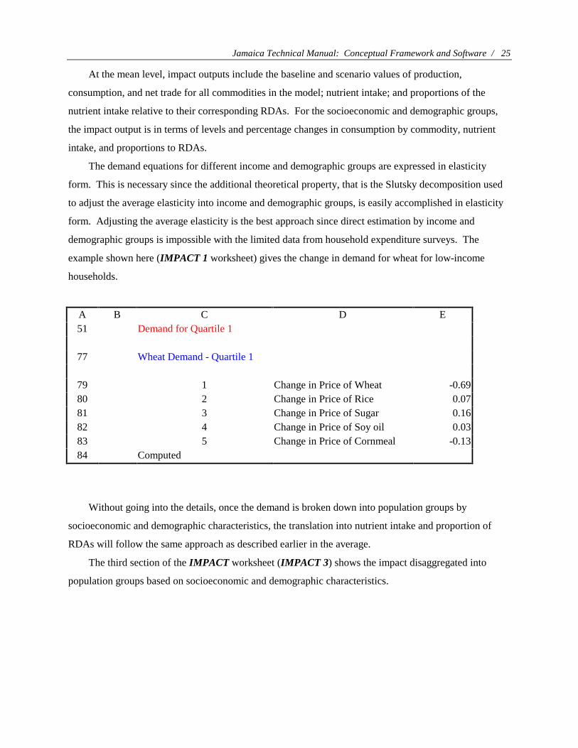
example shown here (IMPACT 1 worksheet) gives the change in demand for wheat for low-income
households.
A B C D E 51 Demand for Quartile 1
77 Wheat Demand - Quartile 1
79 1 Change in Price of Wheat -0.69 80 2 Change in Price of Rice 0.07 81 3 Change in Price of Sugar 0.16 82 4 Change in Price of Soy oil 0.03 83 5 Change in Price of Cornmeal -0.13 84 Computed
Without going into the details, once the demand is broken down into population groups by
socioeconomic and demographic characteristics, the translation into nutrient intake and proportion of
RDAs will follow the same approach as described earlier in the average.
The third section of the IMPACT worksheet (IMPACT 3) shows the impact disaggregated into
population groups based on socioeconomic and demographic characteristics.
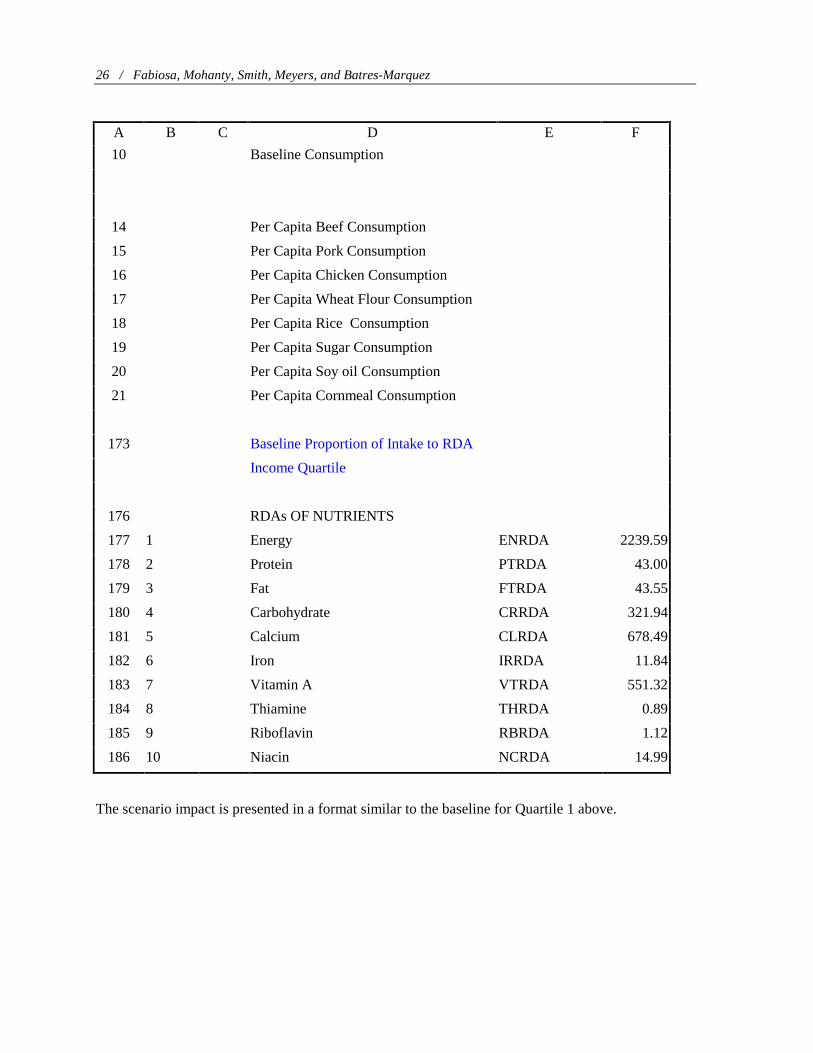
26 / Fabiosa, Mohanty, Smith, Meyers, and Batres-Marquez
A B C D E F
10 Baseline Consumption
14 Per Capita Beef Consumption
15 Per Capita Pork Consumption
16 Per Capita Chicken Consumption
17 Per Capita Wheat Flour Consumption
18 Per Capita Rice Consumption
19 Per Capita Sugar Consumption
20 Per Capita Soy oil Consumption
21 Per Capita Cornmeal Consumption
173 Baseline Proportion of Intake to RDA
Income Quartile
176 RDAs OF NUTRIENTS
177 1 Energy ENRDA 2239.59
178 2 Protein PTRDA 43.00
179 3 Fat FTRDA 43.55
180 4 Carbohydrate CRRDA 321.94
181 5 Calcium CLRDA 678.49
182 6 Iron IRRDA 11.84
183 7 Vitamin A VTRDA 551.32
184 8 Thiamine THRDA 0.89
185 9 Riboflavin RBRDA 1.12
186 10 Niacin NCRDA 14.99
The scenario impact is presented in a format similar to the baseline for Quartile 1 above.

Jamaica Technical Manual: Conceptual Framework and Software / 27
OUTPUT Worksheet
This worksheet summarizes the results from all the worksheets and presents them in a form that can
be easily read and interpreted. For each variable, it provides baseline, scenario, and percentage change
from the baseline. A sample of the summary table for world prices is presented here.
1993 1994 1995 1996 5 World Prices Impact
(US $/MT)
7 8 9
Baseline Wheat Scenario Wheat Percentage Change
140.36 140.36
0
144.00 144.00
0
154.66 156.00
0.86
146.16 150.00
2.63
11 12 13
Baseline Rice Scenario Rice Percentage Change
389.15 389.15
0
457.00 457.00
0
328.73 359.00
9.21
351.02 372.00
5.98
15 16 17
Baseline Sugar Scenario Sugar Percentage Change
220.46 220.46
0
222.31 222.31
0
219.23 219.23
0
219.23 219.23
0
19 20 21
Baseline Soy oil Scenario Soy oil Percentage Change
479.98 479.98
0
597.00 597.00
0
561.28 563.00
0.31
500.08 511.00
2.18
31 32 33
Baseline Corn Scenario Corn Percentage Change
118.96 118.96
0
117.00 117.00
0
96.84 98.00 1.20
101.93 105.00
3.01
35 36 37
Baseline Poultry Scenario Poultry Percentage Change
1217.39 1217.39
0
1228.00 1228.00
0
1144.06 1165.00
1.83
1174.31 1199.00
2.00
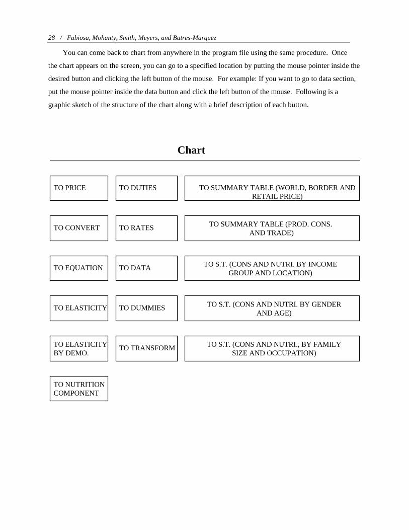
How to Reach the Program Using the Chart
You can also go directly to important sections of the program file by using the chart. Once you load the
program file (FAFSAS.WK4) in Lotus 123, you can reach the chart in three simple steps.
1. Press “Alt-F3” (Macro Run will appear on the screen)
2. Type chart (for Macro name)
3. Press “Enter”
28 / Fabiosa, Mohanty, Smith, Meyers, and Batres-Marquez
You can come back to chart from anywhere in the program file using the same procedure. Once
the chart appears on the screen, you can go to a specified location by putting the mouse pointer inside the
desired button and clicking the left button of the mouse. For example: If you want to go to data section,
put the mouse pointer inside the data button and click the left button of the mouse. Following is a
graphic sketch of the structure of the chart along with a brief description of each button.
TO PRICE TO DUTIES TO SUMMARY TABLE (WORLD, BORDER ANDRETAIL PRICE)
TO CONVERT TO RATES TO SUMMARY TABLE (PROD. CONS. AND TRADE)
TO EQUATION TO DATA TO S.T. (CONS AND NUTRI. BY INCOMEGROUP AND LOCATION)
TO ELASTICITY TO DUMMIES TO S.T. (CONS AND NUTRI. BY GENDERAND AGE)
TO ELASTICITYBY DEMO.
TO TRANSFORM TO S.T. (CONS AND NUTRI., BY FAMILYSIZE AND OCCUPATION)
TO NUTRITIONCOMPONENT
Chart
Jamaica Technical Manual: Conceptual Framework and Software / 29
TO PRICE: Top of Price Section.
TO CONVERT: Section containing various conversion factors.
TO EQUATION: Equation section
TO ELASTICITY: Section having general elasticities estimates
TO ELASTICITY BY DEMO: Section containing elasticities estimates disaggregated by income groups
and demographic characteristics such as income group, location, gender, etc.
TO NUTRITION COMPONENT: Section containing nutrition equations.
TO DUTIES: Contains parameters for policy simulation analysis.
TO RATES: Section that explains tariff structure for various commodities.
TO DATA: Data section
TO DUMMIES: Explains various types of dummies used in the simulation.
TO TRANSFORM: Contains transformed data such budget shares, total
expenditures, etc.
TO SUMMARY TABLE (WORLD, BORDER, AND RETAIL PRICES): Presents summary tables for
world, border and retail prices.
TO SUMMARY TABLE (PROD., CONS. AND TRADE): Presents summary tables of production,
consumption and trade for both crops and livestock.
TO SUMMARY TABLE (CONS. AND NUTRI. BY INCOME GROUP AND LOCAT.): Presents
summary tables of consumption and nutrition impacts for different income groups and locations.
TO SUMMARY TABLE (CONS. AND NUTRI. BY GENDER AND AGE): Presents summary tables of
consumption and nutrition impacts for various gender and age groups .
TO SUMMARY TABLE (CONS. AND NUTRI. BY FAMILY SIZE AND OCCUP.): Presents summary
tables of consumption and nutrition impacts for various family size and occupations.
How to Run the Simulation
Once you load the program file (FAFSAS.WK4) into Lotus 123, go to the chart following the
procedure described earlier (press Alt-F3, type: chart, and press Enter).
When you are in the chart, click the button “TO DUTIES.” That will take you to the “DUTY
SECTION.”
If you are conducting a pure GATT simulation, then enter 0 in C6 (for GATT) or if you are
conducting a GATT run with some changes in the tariff structure, then enter 1 in C6 (for duties).
If you enter 1 in C6, that means you are conducting a simulation with some changes in the tariff
structure, and you need to incorporate the new tariffs. Go to the chart and click on the “RATES” button.

30 / Fabiosa, Mohanty, Smith, Meyers, and Batres-Marquez
Then you type the new tariff values in the “Rate” column. For example: if you are removing the tariffs,
enter 0s in the rate column.
After going through steps 1 to 4, simply press F9 to command Lotus to recalculate all the
worksheets in the program file. The output generated in all the worksheets is automatically summarized
in the OUTPUT worksheet.
CHAPTER 4
Modifying and Updating the Worksheet Program
The worksheet version of the FAFSAS was designed with flexible updating as the primary
consideration. Several possible procedures for alterations are discussed in this chapter.
Availability of New Data
The FAFSAS program lends itself to easy updating when new data is available. The existing
system covers the period from 1972 to 1993. If data for 1994 and 1995 are made available, all that is
needed to incorporate new data into the model is to go to the chart and click the “TO DATA” button.
Once you are in the data section, insert two new columns and enter the data for 1994 and 1995. Then,
the formulas in the equations simply need to be copied to the added columns and the model will
automatically give the new values of all endogenous variables for the added 1994 and 1995 observations.
Reestimation of Equations
If new data for a few years (e.g., three years) are made available, there might be a need to reestimate
the coefficients of the model. Updating the data by adding new columns and copying of formulas similar
to the procedure described above still needs to be done. Also, the new estimated coefficients have to be
inputted into the corresponding equations. That can be done by clicking the button “TO EQUATION”
on the chart. In the equation section, all coefficients are in column E; to “cut and paste” the new
coefficient estimates only the row addresses of the equations are needed. With the updated data and new
coefficients, the model will provide new values of all endogenous variables.
Predicted Values of Exogenous Variables
The solutions of endogenous variables in the CARD/FAPRI International Trade Models are based
on many assumed values of exogenous variables such as unilateral policy changes (e.g., CAP Reform),
multilateral policy changes (e.g., NAFTA and GATT), and macroeconomic assumptions (e.g., project
LINK projections), all of which are updated from year to year. When updated numbers from the
CARD/FAPRI models are made available, they can be directly inputted into the appropriate data

32 / Fabiosa, Mohanty, Smith, Meyers, and Batres-Marquez
addresses. (Go to the data section using the chart and input the new data using the procedure explained
on the previous page.)
New Household Expenditure Survey Data
Household expenditure surveys with national coverage are conducted infrequently. When new
household expenditure survey data are available, elasticities by socioeconomic and demographic
groupings can be adjusted to accommodate the new information. The new elasticities will be entered in
the C column of appropriate row addresses of equations in the impact worksheet.
Nutrient Fortification
Nutrient fortification can be easily accommodated in the model by changing the nutrient availability
per unit of the commodity consumed. A good example is vitamin A fortification in wheat. This will
change the value of vitamin A derived from wheat, which appears in column C.
Additional Commodity Coverage
Increasing the commodity coverage of the model is probably the only change that requires major
modification of the worksheet. It calls for appropriate specification of functional form and choice of
explanatory variables. Coefficients will have to be estimated. New rows will have to be added to
accommodate new functions. The nutrition component will add a new source of nutrients.
Calibrating the Model to Analyze Specific Policy Questions
The model can also be calibrated to analyze specific policy questions that can’t be properly captured
in the present formulation of the worksheet program. This requires conditioning the values of some of
the data in the scenario worksheet to reflect the policy changes. The relevant equations affected by these
data will then have to be instructed to feed from this newly constructed data series. The structure of the
BASELINE and IMPACT worksheets remains as is and captures the effect of the new policy(ies).
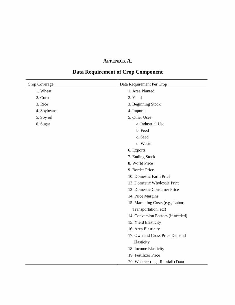
APPENDIX A.
Data Requirement of Crop Component
Crop Coverage Data Requirement Per Crop
1. Wheat
2. Corn
3. Rice
4. Soybeans
5. Soy oil
6. Sugar
1. Area Planted
2. Yield
3. Beginning Stock
4. Imports
5. Other Uses
a. Industrial Use
b. Feed
c. Seed
d. Waste
6. Exports
7. Ending Stock
8. World Price
9. Border Price
10. Domestic Farm Price
12. Domestic Wholesale Price
13. Domestic Consumer Price
14. Price Margins
15. Marketing Costs (e.g., Labor,
Transportation, etc)
14. Conversion Factors (if needed)
15. Yield Elasticity
16. Area Elasticity
17. Own and Cross Price Demand
Elasticity
18. Income Elasticity
19. Fertilizer Price
20. Weather (e.g., Rainfall) Data
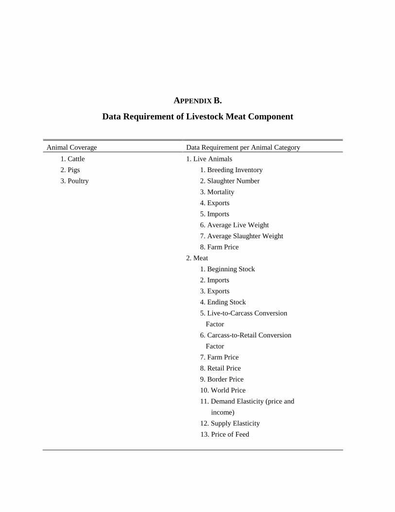
APPENDIX B.
Data Requirement of Livestock Meat Component
Animal Coverage Data Requirement per Animal Category
1. Cattle
2. Pigs
3. Poultry
1. Live Animals
1. Breeding Inventory
2. Slaughter Number
3. Mortality
4. Exports
5. Imports
6. Average Live Weight
7. Average Slaughter Weight
8. Farm Price
2. Meat
1. Beginning Stock
2. Imports
3. Exports
4. Ending Stock
5. Live-to-Carcass Conversion
Factor
6. Carcass-to-Retail Conversion
Factor
7. Farm Price
8. Retail Price
9. Border Price
10. World Price
11. Demand Elasticity (price and
income)
12. Supply Elasticity
13. Price of Feed
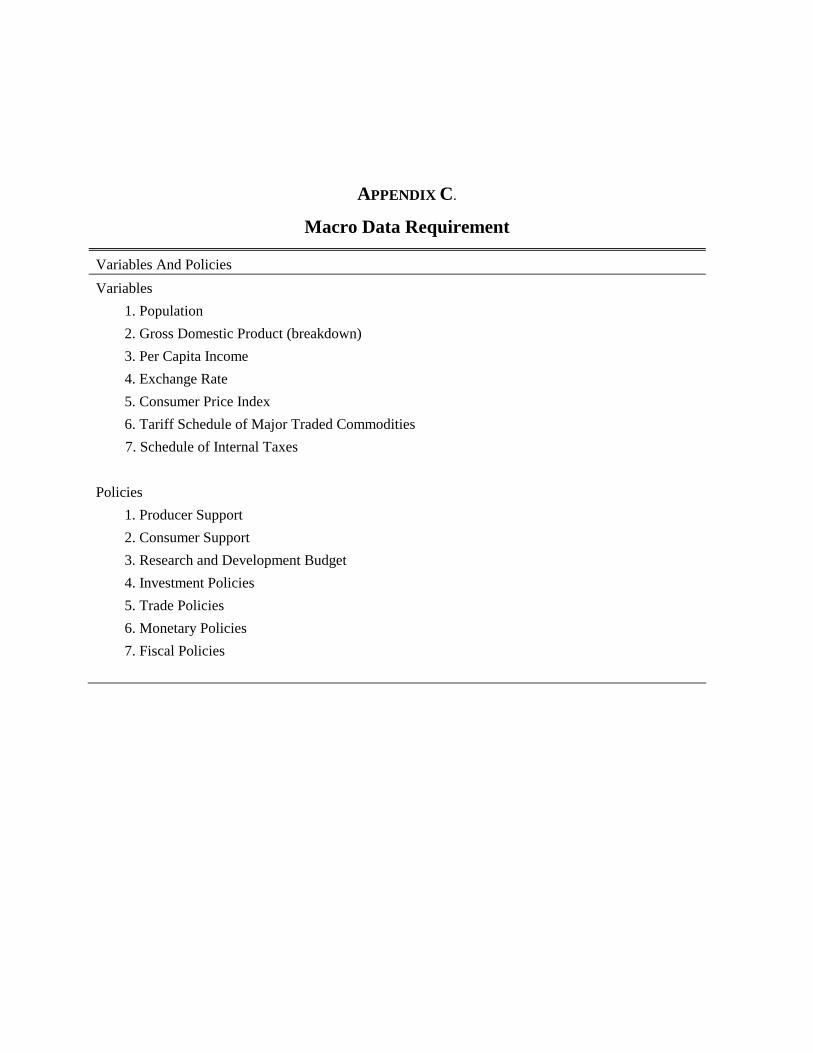
APPENDIX C.
Macro Data Requirement
Variables And Policies
Variables
1. Population
2. Gross Domestic Product (breakdown)
3. Per Capita Income
4. Exchange Rate
5. Consumer Price Index
6. Tariff Schedule of Major Traded Commodities
7. Schedule of Internal Taxes
Policies
1. Producer Support
2. Consumer Support
3. Research and Development Budget
4. Investment Policies
5. Trade Policies
6. Monetary Policies
7. Fiscal Policies
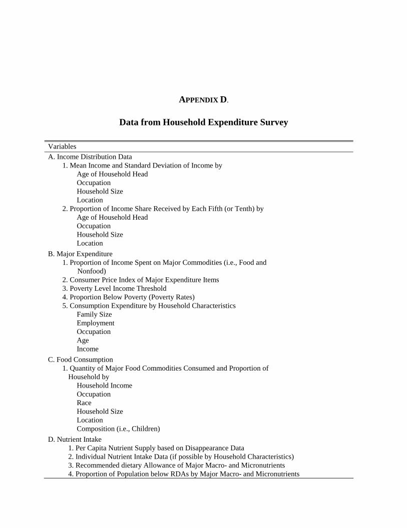
APPENDIX D.
Data from Household Expenditure Survey
Variables
A. Income Distribution Data 1. Mean Income and Standard Deviation of Income by Age of Household Head Occupation Household Size Location 2. Proportion of Income Share Received by Each Fifth (or Tenth) by Age of Household Head Occupation Household Size Location
B. Major Expenditure 1. Proportion of Income Spent on Major Commodities (i.e., Food and Nonfood) 2. Consumer Price Index of Major Expenditure Items 3. Poverty Level Income Threshold 4. Proportion Below Poverty (Poverty Rates) 5. Consumption Expenditure by Household Characteristics Family Size Employment Occupation Age Income
C. Food Consumption 1. Quantity of Major Food Commodities Consumed and Proportion of Household by Household Income Occupation Race Household Size Location Composition (i.e., Children)
D. Nutrient Intake 1. Per Capita Nutrient Supply based on Disappearance Data 2. Individual Nutrient Intake Data (if possible by Household Characteristics) 3. Recommended dietary Allowance of Major Macro- and Micronutrients 4. Proportion of Population below RDAs by Major Macro- and Micronutrients
APPENDIX E.
Theoretical Framework of Supply and Demand Functions
Consumers are modeled as maximizing utility subject to some budget constraint. A representative
consumer cost function is given in
� �E1 ln ( , ) ( ) ( ).C P U a P b P U� � ,
where
� �E2 a P p p pi ii
ij i jji
( ) ln ln ln� � �� ��� � �0
1
2
and
� �E3 b P pkk
nk( ) �
�
� �
01 .
The demand function is derived using Hotelling’s Lemma. That is, taking the first derivative of [E1]
gives the Hicksian demand and substituting out U gives the Marshallian demand, the Almost Ideal
Demand System (AIDS). The resulting demand function is of the form,
� �E4 w pX
Pi i ij j ij
� � � ��
���� � �ln ln
where ln(P) is approximated by a Stone Price Index.
From standard microeconomic theory, the supply function is derived from an indirect profit
function. That is,
� �E5 � ( , ) . ( , )p y p y c y w� � ,
the optimal y* = y(p,w) is substituted in [E5] to get the indirect profit function:
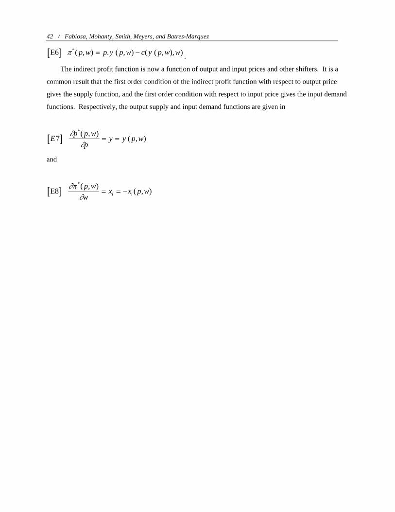
42 / Fabiosa, Mohanty, Smith, Meyers, and Batres-Marquez
� �E6 � *( , ) . ( , ) ( ( , ), )p w p y p w c y p w w� � .
The indirect profit function is now a function of output and input prices and other shifters. It is a
common result that the first order condition of the indirect profit function with respect to output price
gives the supply function, and the first order condition with respect to input price gives the input demand
functions. Respectively, the output supply and input demand functions are given in
� �Ep p w
py y p w7
( , ) ( , )
*��
� �
and
� �E8 ��
�
*( , )( , )
p w
wx x p wi i� � �
APPENDIX F.
Parameter Estimates
Table 1. Parameter Estimates of Meat Demand Variable Coefficient Standard Error
DEPENDENT
Share of Beef
INDEPENDENT
Constant 0.834 0.172
Log of Price of Beef -0.077 0.022
Log of Price of Chicken -0.033 0.020
Log of Real Expenditure -0.071 0.039
First Difference of Beef Share 0.276 0.042
Second Difference of Beef Share 0.252 0.031
First Difference of Price of Beef 0.054 0.049
First Difference of Price of Chicken 0.014 0.023
First Difference of Price of Pork -0.050 0.042
Trend -0.013 0.001
DEPENDENT
Share of Chicken
INDEPENDENT
Constant -0.336 0.185
Log Price of Chicken 0.093 0.022
Log of Real Expenditure 0.179 0.042
First Difference of Chicken Share 0.222 0.039
Second Difference of Chicken Share 0.165 0.027
First Difference Price of Beef -0.071 0.053
First Difference Price of Chicken -0.034 0.025
First Difference Price of Pork 0.073 0.044
Trend 0.012 0.001
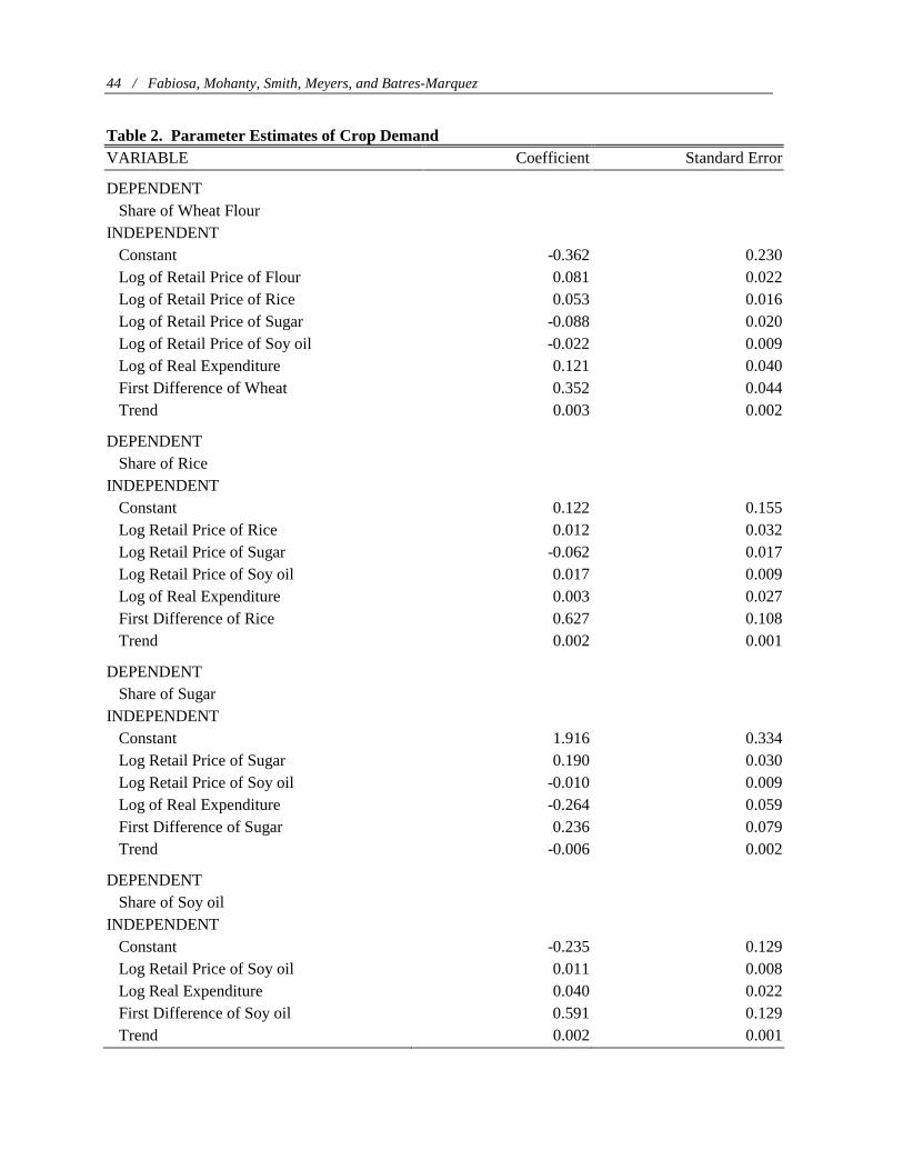
44 / Fabiosa, Mohanty, Smith, Meyers, and Batres-Marquez
Table 2. Parameter Estimates of Crop Demand VARIABLE Coefficient Standard Error
DEPENDENT Share of Wheat Flour INDEPENDENT Constant -0.362 0.230 Log of Retail Price of Flour 0.081 0.022 Log of Retail Price of Rice 0.053 0.016 Log of Retail Price of Sugar -0.088 0.020 Log of Retail Price of Soy oil -0.022 0.009 Log of Real Expenditure 0.121 0.040 First Difference of Wheat 0.352 0.044 Trend 0.003 0.002
DEPENDENT Share of Rice INDEPENDENT Constant 0.122 0.155 Log Retail Price of Rice 0.012 0.032 Log Retail Price of Sugar -0.062 0.017 Log Retail Price of Soy oil 0.017 0.009 Log of Real Expenditure 0.003 0.027 First Difference of Rice 0.627 0.108 Trend 0.002 0.001
DEPENDENT Share of Sugar INDEPENDENT Constant 1.916 0.334 Log Retail Price of Sugar 0.190 0.030 Log Retail Price of Soy oil -0.010 0.009 Log of Real Expenditure -0.264 0.059 First Difference of Sugar 0.236 0.079 Trend -0.006 0.002
DEPENDENT Share of Soy oil INDEPENDENT Constant -0.235 0.129 Log Retail Price of Soy oil 0.011 0.008 Log Real Expenditure 0.040 0.022 First Difference of Soy oil 0.591 0.129 Trend 0.002 0.001
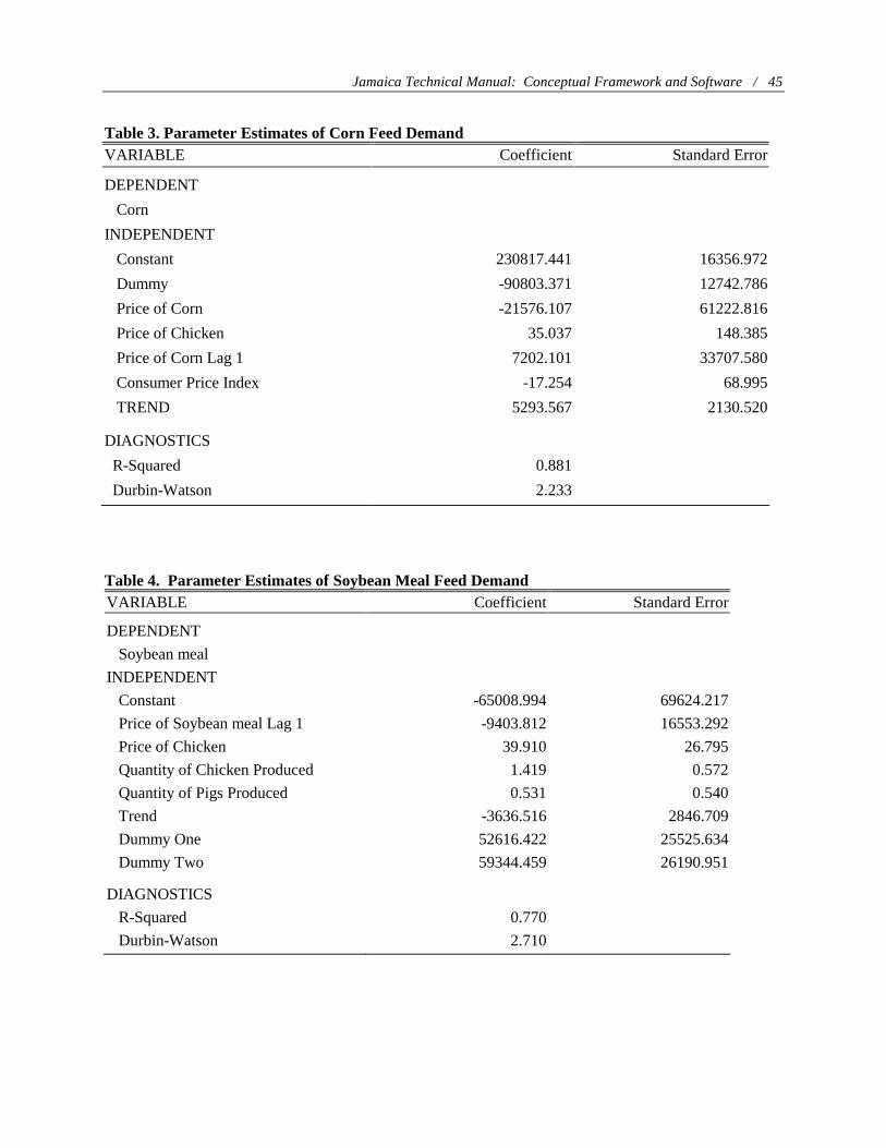
Jamaica Technical Manual: Conceptual Framework and Software / 45
Table 3. Parameter Estimates of Corn Feed Demand VARIABLE Coefficient Standard Error
DEPENDENT
Corn
INDEPENDENT
Constant 230817.441 16356.972
Dummy -90803.371 12742.786
Price of Corn -21576.107 61222.816
Price of Chicken 35.037 148.385
Price of Corn Lag 1 7202.101 33707.580
Consumer Price Index -17.254 68.995
TREND 5293.567 2130.520
DIAGNOSTICS
R-Squared 0.881
Durbin-Watson 2.233
Table 4. Parameter Estimates of Soybean Meal Feed Demand VARIABLE Coefficient Standard Error
DEPENDENT
Soybean meal
INDEPENDENT
Constant -65008.994 69624.217
Price of Soybean meal Lag 1 -9403.812 16553.292
Price of Chicken 39.910 26.795
Quantity of Chicken Produced 1.419 0.572
Quantity of Pigs Produced 0.531 0.540
Trend -3636.516 2846.709
Dummy One 52616.422 25525.634
Dummy Two 59344.459 26190.951
DIAGNOSTICS
R-Squared 0.770
Durbin-Watson 2.710
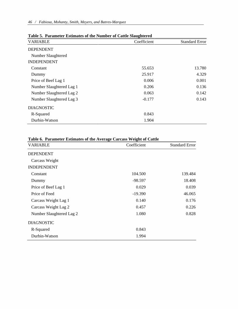
46 / Fabiosa, Mohanty, Smith, Meyers, and Batres-Marquez
Table 5. Parameter Estimates of the Number of Cattle Slaughtered VARIABLE Coefficient Standard Error
DEPENDENT
Number Slaughtered
INDEPENDENT
Constant 55.653 13.780
Dummy 25.917 4.329
Price of Beef Lag 1 0.006 0.001
Number Slaughtered Lag 1 0.206 0.136
Number Slaughtered Lag 2 0.063 0.142
Number Slaughtered Lag 3 -0.177 0.143
DIAGNOSTIC
R-Squared 0.843
Durbin-Watson 1.904
Table 6. Parameter Estimates of the Average Carcass Weight of Cattle VARIABLE Coefficient Standard Error
DEPENDENT
Carcass Weight
INDEPENDENT
Constant 104.500 139.484
Dummy -98.597 18.408
Price of Beef Lag 1 0.029 0.039
Price of Feed -19.390 46.065
Carcass Weight Lag 1 0.140 0.176
Carcass Weight Lag 2 0.457 0.226
Number Slaughtered Lag 2 1.080 0.828
DIAGNOSTIC
R-Squared 0.843
Durbin-Watson 1.994
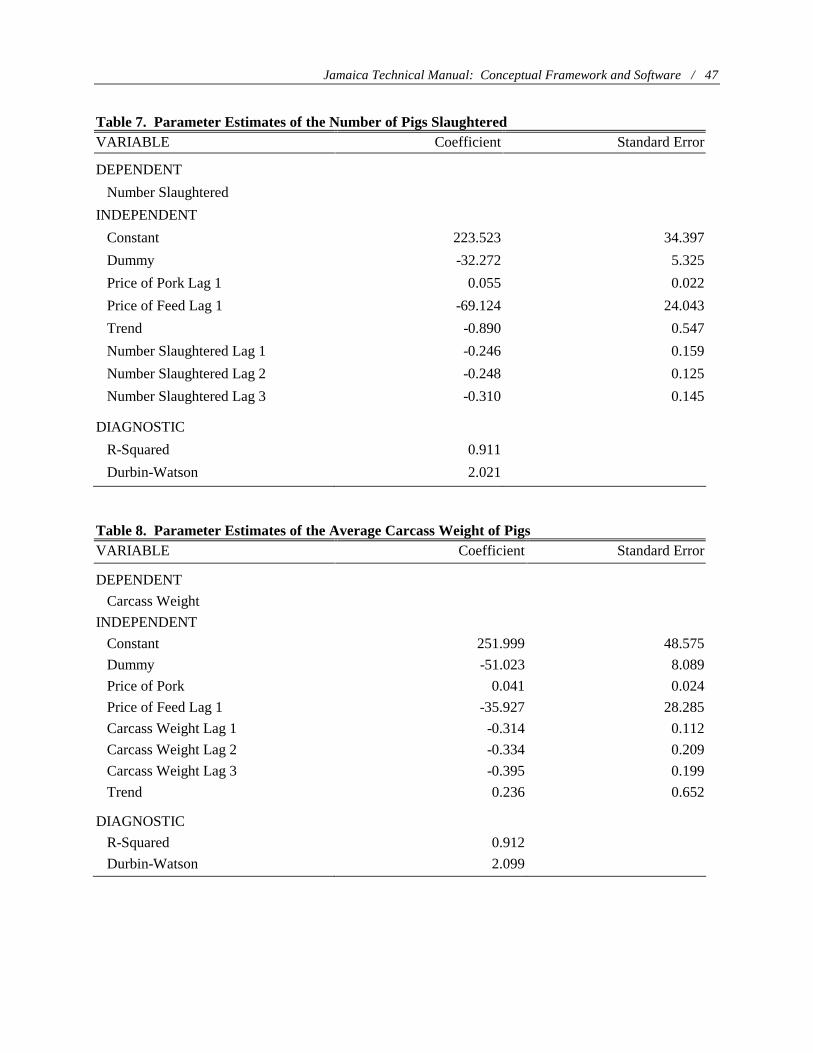
Jamaica Technical Manual: Conceptual Framework and Software / 47
Table 7. Parameter Estimates of the Number of Pigs Slaughtered VARIABLE Coefficient Standard Error
DEPENDENT
Number Slaughtered
INDEPENDENT
Constant 223.523 34.397
Dummy -32.272 5.325
Price of Pork Lag 1 0.055 0.022
Price of Feed Lag 1 -69.124 24.043
Trend -0.890 0.547
Number Slaughtered Lag 1 -0.246 0.159
Number Slaughtered Lag 2 -0.248 0.125
Number Slaughtered Lag 3 -0.310 0.145
DIAGNOSTIC
R-Squared 0.911
Durbin-Watson 2.021
Table 8. Parameter Estimates of the Average Carcass Weight of Pigs VARIABLE Coefficient Standard Error
DEPENDENT
Carcass Weight
INDEPENDENT
Constant 251.999 48.575
Dummy -51.023 8.089
Price of Pork 0.041 0.024
Price of Feed Lag 1 -35.927 28.285
Carcass Weight Lag 1 -0.314 0.112
Carcass Weight Lag 2 -0.334 0.209
Carcass Weight Lag 3 -0.395 0.199
Trend 0.236 0.652
DIAGNOSTIC
R-Squared 0.912
Durbin-Watson 2.099
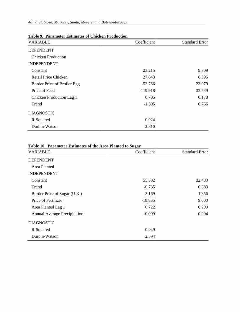
48 / Fabiosa, Mohanty, Smith, Meyers, and Batres-Marquez
Table 9. Parameter Estimates of Chicken Production VARIABLE Coefficient Standard Error
DEPENDENT
Chicken Production
INDEPENDENT
Constant 23.215 9.309
Retail Price Chicken 27.843 6.395
Border Price of Broiler Egg -52.786 23.079
Price of Feed -119.918 32.549
Chicken Production Lag 1 0.705 0.178
Trend -1.305 0.766
DIAGNOSTIC
R-Squared 0.924
Durbin-Watson 2.810
Table 10. Parameter Estimates of the Area Planted to Sugar VARIABLE Coefficient Standard Error
DEPENDENT
Area Planted
INDEPENDENT
Constant 55.382 32.480
Trend -0.735 0.883
Border Price of Sugar (U.K.) 3.169 1.356
Price of Fertilizer -19.835 9.000
Area Planted Lag 1 0.722 0.200
Annual Average Precipitation -0.009 0.004
DIAGNOSTIC
R-Squared 0.949
Durbin-Watson 2.594
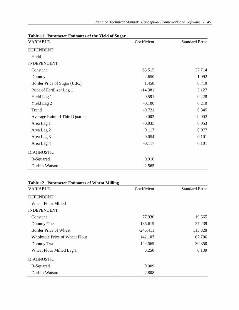
Jamaica Technical Manual: Conceptual Framework and Software / 49
Table 11. Parameter Estimates of the Yield of Sugar VARIABLE Coefficient Standard Error
DEPENDENT
Yield
INDEPENDENT
Constant 63.515 27.714
Dummy -2.650 1.092
Border Price of Sugar (U.K.) 1.458 0.710
Price of Fertilizer Lag 1 -14.381 3.127
Yield Lag 1 -0.591 0.228
Yield Lag 2 -0.100 0.210
Trend -0.721 0.845
Average Rainfall Third Quarter 0.002 0.002
Area Lag 1 -0.035 0.053
Area Lag 2 0.117 0.077
Area Lag 3 -0.054 0.101
Area Lag 4 -0.117 0.101
DIAGNOSTIC
R-Squared 0.910
Durbin-Watson 2.565
Table 12. Parameter Estimates of Wheat Milling VARIABLE Coefficient Standard Error
DEPENDENT
Wheat Flour Milled
INDEPENDENT
Constant 77.936 19.565
Dummy One 135.619 27.239
Border Price of Wheat -246.411 113.328
Wholesale Price of Wheat Flour 142.107 67.706
Dummy Two -144.569 30.350
Wheat Flour Milled Lag 1 0.250 0.139
DIAGNOSTIC
R-Squared 0.909
Durbin-Watson 2.808
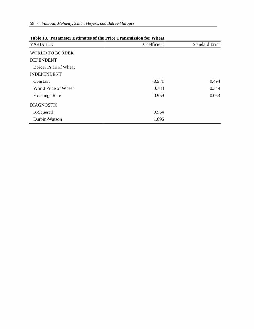
50 / Fabiosa, Mohanty, Smith, Meyers, and Batres-Marquez
Table 13. Parameter Estimates of the Price Transmission for Wheat VARIABLE Coefficient Standard Error
WORLD TO BORDER
DEPENDENT
Border Price of Wheat
INDEPENDENT
Constant -3.571 0.494
World Price of Wheat 0.788 0.349
Exchange Rate 0.959 0.053
DIAGNOSTIC
R-Squared 0.954
Durbin-Watson 1.696
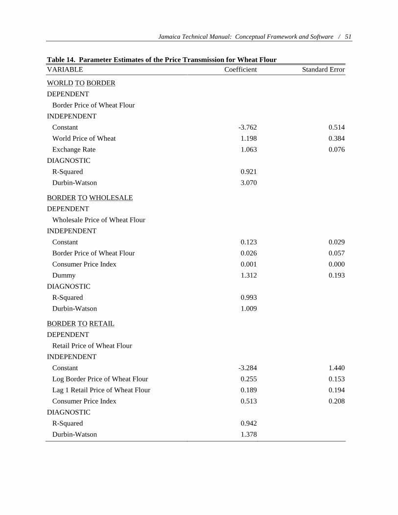
Jamaica Technical Manual: Conceptual Framework and Software / 51
Table 14. Parameter Estimates of the Price Transmission for Wheat Flour VARIABLE Coefficient Standard Error
WORLD TO BORDER
DEPENDENT
Border Price of Wheat Flour
INDEPENDENT
Constant -3.762 0.514
World Price of Wheat 1.198 0.384
Exchange Rate 1.063 0.076
DIAGNOSTIC
R-Squared 0.921
Durbin-Watson 3.070
BORDER TO WHOLESALE
DEPENDENT
Wholesale Price of Wheat Flour
INDEPENDENT
Constant 0.123 0.029
Border Price of Wheat Flour 0.026 0.057
Consumer Price Index 0.001 0.000
Dummy 1.312 0.193
DIAGNOSTIC
R-Squared 0.993
Durbin-Watson 1.009
BORDER TO RETAIL
DEPENDENT
Retail Price of Wheat Flour
INDEPENDENT
Constant -3.284 1.440
Log Border Price of Wheat Flour 0.255 0.153
Lag 1 Retail Price of Wheat Flour 0.189 0.194
Consumer Price Index 0.513 0.208
DIAGNOSTIC
R-Squared 0.942
Durbin-Watson 1.378
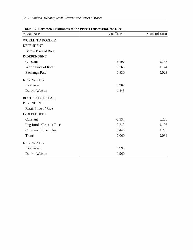
52 / Fabiosa, Mohanty, Smith, Meyers, and Batres-Marquez
Table 15. Parameter Estimates of the Price Transmission for Rice VARIABLE Coefficient Standard Error
WORLD TO BORDER
DEPENDENT
Border Price of Rice
INDEPENDENT
Constant -6.107 0.735
World Price of Rice 0.765 0.124
Exchange Rate 0.830 0.023
DIAGNOSTIC
R-Squared 0.987
Durbin-Watson 1.843
BORDER TO RETAIL
DEPENDENT
Retail Price of Rice
INDEPENDENT
Constant -3.337 1.235
Log Border Price of Rice 0.242 0.136
Consumer Price Index 0.443 0.253
Trend 0.060 0.034
DIAGNOSTIC
R-Squared 0.990
Durbin-Watson 1.960
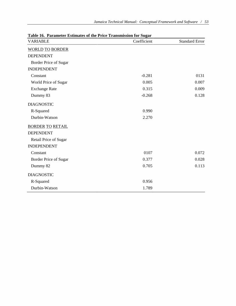
Jamaica Technical Manual: Conceptual Framework and Software / 53
Table 16. Parameter Estimates of the Price Transmission for Sugar VARIABLE Coefficient Standard Error
WORLD TO BORDER
DEPENDENT
Border Price of Sugar
INDEPENDENT
Constant -0.281 0131
World Price of Sugar 0.005 0.007
Exchange Rate 0.315 0.009
Dummy 83 -0.268 0.128
DIAGNOSTIC
R-Squared 0.990
Durbin-Watson 2.270
BORDER TO RETAIL
DEPENDENT
Retail Price of Sugar
INDEPENDENT
Constant 0107 0.072
Border Price of Sugar 0.377 0.028
Dummy 82 0.705 0.113
DIAGNOSTIC
R-Squared 0.956
Durbin-Watson 1.789
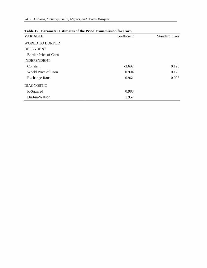
54 / Fabiosa, Mohanty, Smith, Meyers, and Batres-Marquez
Table 17. Parameter Estimates of the Price Transmission for Corn VARIABLE Coefficient Standard Error
WORLD TO BORDER
DEPENDENT
Border Price of Corn
INDEPENDENT
Constant -3.692 0.125
World Price of Corn 0.904 0.125
Exchange Rate 0.961 0.025
DIAGNOSTIC
R-Squared 0.988
Durbin-Watson 1.957
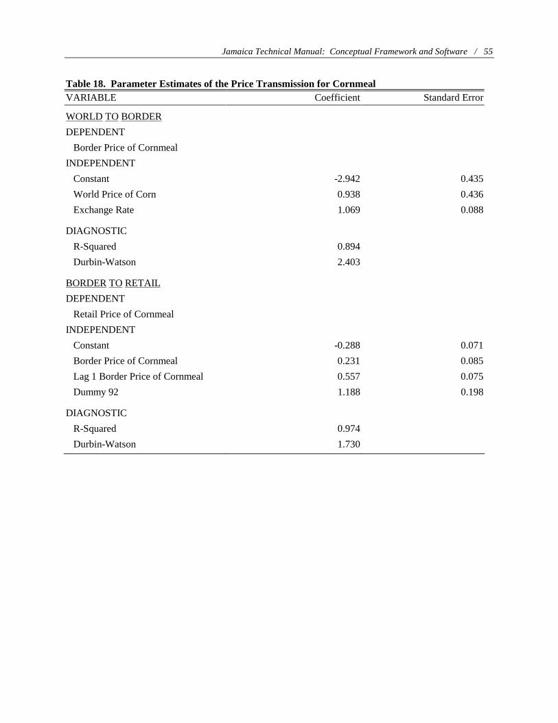
Jamaica Technical Manual: Conceptual Framework and Software / 55
Table 18. Parameter Estimates of the Price Transmission for Cornmeal VARIABLE Coefficient Standard Error
WORLD TO BORDER
DEPENDENT
Border Price of Cornmeal
INDEPENDENT
Constant -2.942 0.435
World Price of Corn 0.938 0.436
Exchange Rate 1.069 0.088
DIAGNOSTIC
R-Squared 0.894
Durbin-Watson 2.403
BORDER TO RETAIL
DEPENDENT
Retail Price of Cornmeal
INDEPENDENT
Constant -0.288 0.071
Border Price of Cornmeal 0.231 0.085
Lag 1 Border Price of Cornmeal 0.557 0.075
Dummy 92 1.188 0.198
DIAGNOSTIC
R-Squared 0.974
Durbin-Watson 1.730
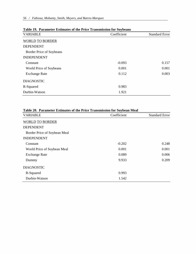
56 / Fabiosa, Mohanty, Smith, Meyers, and Batres-Marquez
Table 19. Parameter Estimates of the Price Transmission for Soybeans VARIABLE Coefficient Standard Error
WORLD TO BORDER
DEPENDENT
Border Price of Soybeans
INDEPENDENT
Constant -0.093 0.157
World Price of Soybeans 0.001 0.001
Exchange Rate 0.112 0.003
DIAGNOSTIC
R-Squared 0.983
Durbin-Watson 1.921
Table 20. Parameter Estimates of the Price Transmission for Soybean Meal VARIABLE Coefficient Standard Error
WORLD TO BORDER
DEPENDENT
Border Price of Soybean Meal
INDEPENDENT
Constant -0.202 0.248
World Price of Soybean Meal 0.001 0.001
Exchange Rate 0.089 0.006
Dummy 9.933 0.209
DIAGNOSTIC
R-Squared 0.993
Durbin-Watson 1.542
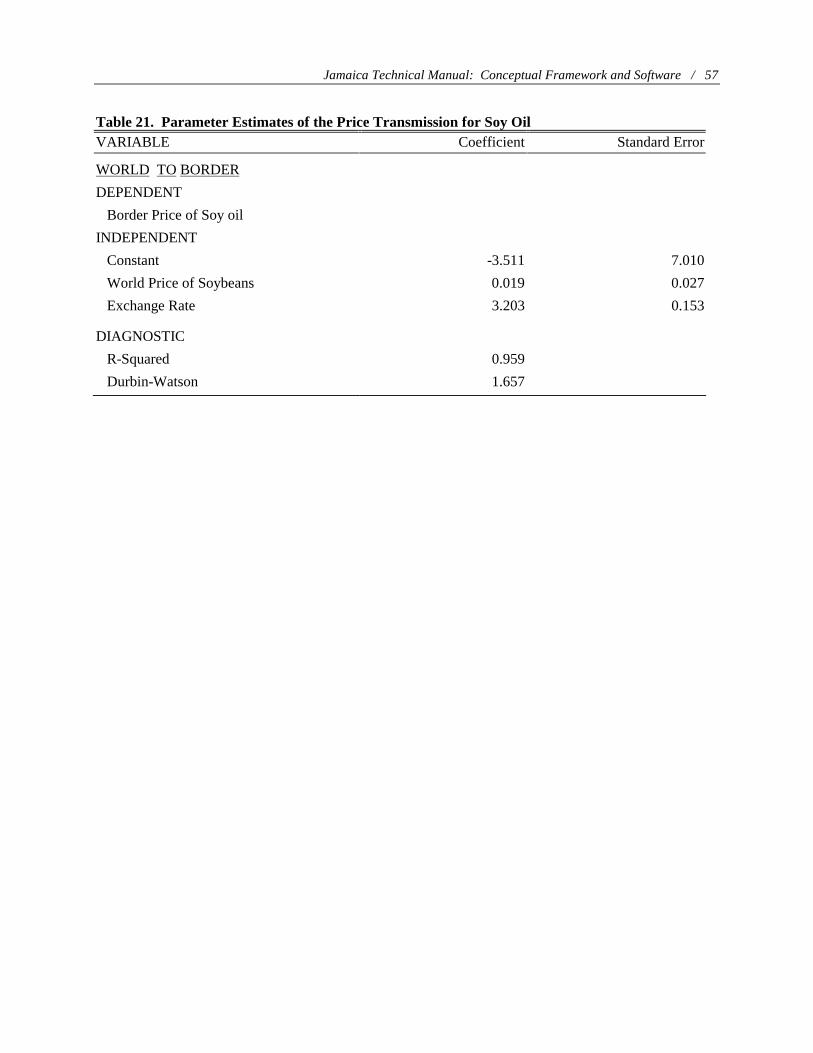
Jamaica Technical Manual: Conceptual Framework and Software / 57
Table 21. Parameter Estimates of the Price Transmission for Soy Oil VARIABLE Coefficient Standard Error
WORLD TO BORDER
DEPENDENT
Border Price of Soy oil
INDEPENDENT
Constant -3.511 7.010
World Price of Soybeans 0.019 0.027
Exchange Rate 3.203 0.153
DIAGNOSTIC
R-Squared 0.959
Durbin-Watson 1.657
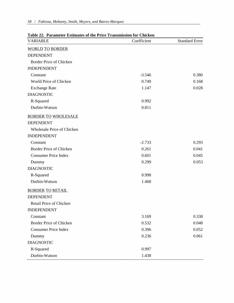
58 / Fabiosa, Mohanty, Smith, Meyers, and Batres-Marquez
Table 22. Parameter Estimates of the Price Transmission for Chicken VARIABLE Coefficient Standard Error
WORLD TO BORDER
DEPENDENT
Border Price of Chicken
INDEPENDENT
Constant -3.546 0.380
World Price of Chicken 0.749 0.168
Exchange Rate 1.147 0.028
DIAGNOSTIC
R-Squared 0.992
Durbin-Watson 0.811
BORDER TO WHOLESALE
DEPENDENT
Wholesale Price of Chicken
INDEPENDENT
Constant -2.733 0.293
Border Price of Chicken 0.261 0.041
Consumer Price Index 0.601 0.045
Dummy 0.299 0.053
DIAGNOSTIC
R-Squared 0.998
Durbin-Watson 1.468
BORDER TO RETAIL
DEPENDENT
Retail Price of Chicken
INDEPENDENT
Constant 3.169 0.338
Border Price of Chicken 0.532 0.048
Consumer Price Index 0.396 0.052
Dummy 0.236 0.061
DIAGNOSTIC
R-Squared 0.997
Durbin-Watson 1.438
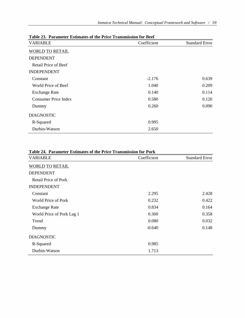
Jamaica Technical Manual: Conceptual Framework and Software / 59
Table 23. Parameter Estimates of the Price Transmission for Beef VARIABLE Coefficient Standard Error
WORLD TO RETAIL
DEPENDENT
Retail Price of Beef
INDEPENDENT
Constant -2.176 0.639
World Price of Beef 1.040 0.209
Exchange Rate 0.140 0.114
Consumer Price Index 0.580 0.120
Dummy 0.260 0.090
DIAGNOSTIC
R-Squared 0.995
Durbin-Watson 2.650
Table 24. Parameter Estimates of the Price Transmission for Pork VARIABLE Coefficient Standard Error
WORLD TO RETAIL
DEPENDENT
Retail Price of Pork
INDEPENDENT
Constant 2.295 2.428
World Price of Pork 0.232 0.422
Exchange Rate 0.834 0.164
World Price of Pork Lag 1 0.300 0.358
Trend 0.080 0.032
Dummy -0.640 0.148
DIAGNOSTIC
R-Squared 0.985
Durbin-Watson 1.713

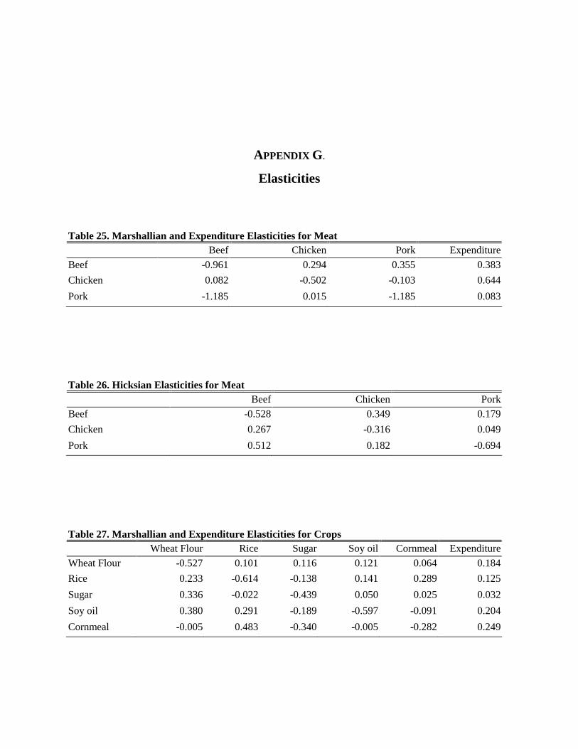
APPENDIX G.
Elasticities
Table 25. Marshallian and Expenditure Elasticities for Meat
Beef Chicken Pork Expenditure
Beef -0.961 0.294 0.355 0.383
Chicken 0.082 -0.502 -0.103 0.644
Pork -1.185 0.015 -1.185 0.083
Table 26. Hicksian Elasticities for Meat
Beef Chicken Pork
Beef -0.528 0.349 0.179
Chicken 0.267 -0.316 0.049
Pork 0.512 0.182 -0.694
Table 27. Marshallian and Expenditure Elasticities for Crops
Wheat Flour Rice Sugar Soy oil Cornmeal Expenditure
Wheat Flour -0.527 0.101 0.116 0.121 0.064 0.184
Rice 0.233 -0.614 -0.138 0.141 0.289 0.125
Sugar 0.336 -0.022 -0.439 0.050 0.025 0.032
Soy oil 0.380 0.291 -0.189 -0.597 -0.091 0.204
Cornmeal -0.005 0.483 -0.340 -0.005 -0.282 0.249
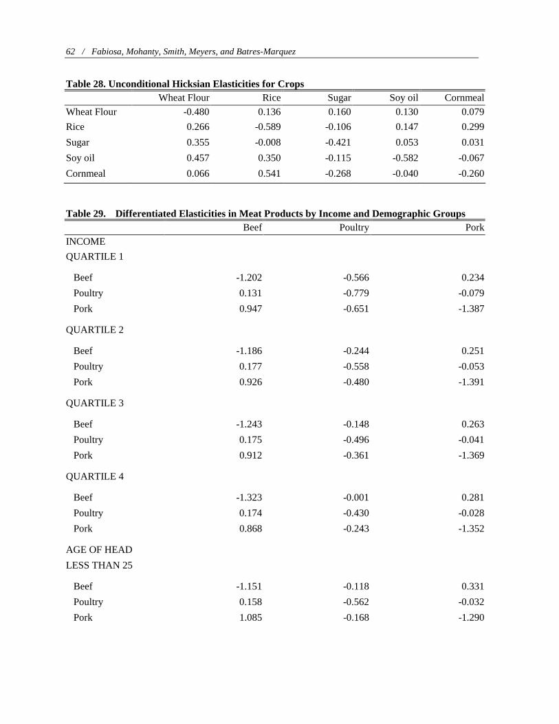
62 / Fabiosa, Mohanty, Smith, Meyers, and Batres-Marquez
Table 28. Unconditional Hicksian Elasticities for Crops
Wheat Flour Rice Sugar Soy oil Cornmeal
Wheat Flour -0.480 0.136 0.160 0.130 0.079
Rice 0.266 -0.589 -0.106 0.147 0.299
Sugar 0.355 -0.008 -0.421 0.053 0.031
Soy oil 0.457 0.350 -0.115 -0.582 -0.067
Cornmeal 0.066 0.541 -0.268 -0.040 -0.260
Table 29. Differentiated Elasticities in Meat Products by Income and Demographic Groups Beef Poultry Pork
INCOME
QUARTILE 1
Beef -1.202 -0.566 0.234
Poultry 0.131 -0.779 -0.079
Pork 0.947 -0.651 -1.387
QUARTILE 2
Beef -1.186 -0.244 0.251
Poultry 0.177 -0.558 -0.053
Pork 0.926 -0.480 -1.391
QUARTILE 3
Beef -1.243 -0.148 0.263
Poultry 0.175 -0.496 -0.041
Pork 0.912 -0.361 -1.369
QUARTILE 4
Beef -1.323 -0.001 0.281
Poultry 0.174 -0.430 -0.028
Pork 0.868 -0.243 -1.352
AGE OF HEAD
LESS THAN 25
Beef -1.151 -0.118 0.331
Poultry 0.158 -0.562 -0.032
Pork 1.085 -0.168 -1.290
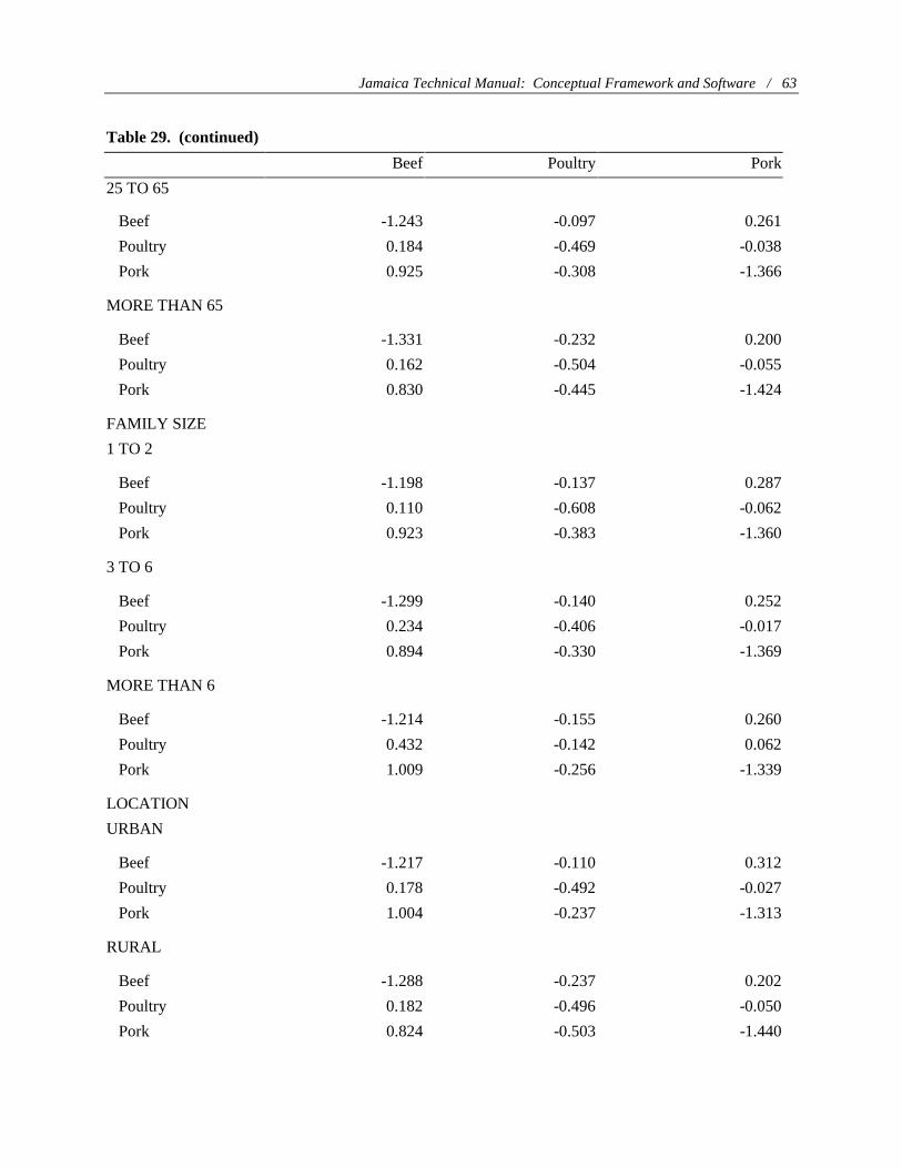
Jamaica Technical Manual: Conceptual Framework and Software / 63
Table 29. (continued)
Beef Poultry Pork
25 TO 65
Beef -1.243 -0.097 0.261
Poultry 0.184 -0.469 -0.038
Pork 0.925 -0.308 -1.366
MORE THAN 65
Beef -1.331 -0.232 0.200
Poultry 0.162 -0.504 -0.055
Pork 0.830 -0.445 -1.424
FAMILY SIZE
1 TO 2
Beef -1.198 -0.137 0.287
Poultry 0.110 -0.608 -0.062
Pork 0.923 -0.383 -1.360
3 TO 6
Beef -1.299 -0.140 0.252
Poultry 0.234 -0.406 -0.017
Pork 0.894 -0.330 -1.369
MORE THAN 6
Beef -1.214 -0.155 0.260
Poultry 0.432 -0.142 0.062
Pork 1.009 -0.256 -1.339
LOCATION
URBAN
Beef -1.217 -0.110 0.312
Poultry 0.178 -0.492 -0.027
Pork 1.004 -0.237 -1.313
RURAL
Beef -1.288 -0.237 0.202
Poultry 0.182 -0.496 -0.050
Pork 0.824 -0.503 -1.440
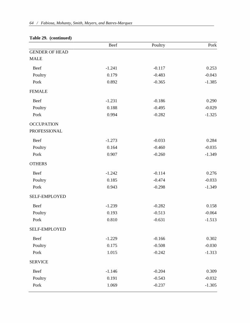
64 / Fabiosa, Mohanty, Smith, Meyers, and Batres-Marquez
Table 29. (continued)
Beef Poultry Pork
GENDER OF HEAD
MALE
Beef -1.241 -0.117 0.253
Poultry 0.179 -0.483 -0.043
Pork 0.892 -0.365 -1.385
FEMALE
Beef -1.231 -0.186 0.290
Poultry 0.188 -0.495 -0.029
Pork 0.994 -0.282 -1.325
OCCUPATION
PROFESSIONAL
Beef -1.273 -0.033 0.284
Poultry 0.164 -0.460 -0.035
Pork 0.907 -0.260 -1.349
OTHERS
Beef -1.242 -0.114 0.276
Poultry 0.185 -0.474 -0.033
Pork 0.943 -0.298 -1.349
SELF-EMPLOYED
Beef -1.239 -0.282 0.158
Poultry 0.193 -0.513 -0.064
Pork 0.810 -0.631 -1.513
SELF-EMPLOYED
Beef -1.229 -0.166 0.302
Poultry 0.175 -0.508 -0.030
Pork 1.015 -0.242 -1.313
SERVICE
Beef -1.146 -0.204 0.309
Poultry 0.191 -0.543 -0.032
Pork 1.069 -0.237 -1.305
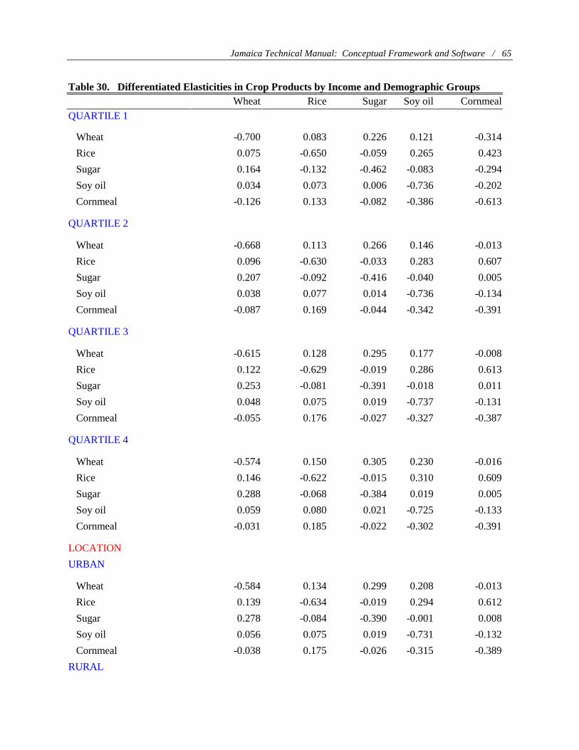
Jamaica Technical Manual: Conceptual Framework and Software / 65
Table 30. Differentiated Elasticities in Crop Products by Income and Demographic Groups Wheat Rice Sugar Soy oil Cornmeal
QUARTILE 1
Wheat -0.700 0.083 0.226 0.121 -0.314
Rice 0.075 -0.650 -0.059 0.265 0.423
Sugar 0.164 -0.132 -0.462 -0.083 -0.294
Soy oil 0.034 0.073 0.006 -0.736 -0.202
Cornmeal -0.126 0.133 -0.082 -0.386 -0.613
QUARTILE 2
Wheat -0.668 0.113 0.266 0.146 -0.013
Rice 0.096 -0.630 -0.033 0.283 0.607
Sugar 0.207 -0.092 -0.416 -0.040 0.005
Soy oil 0.038 0.077 0.014 -0.736 -0.134
Cornmeal -0.087 0.169 -0.044 -0.342 -0.391
QUARTILE 3
Wheat -0.615 0.128 0.295 0.177 -0.008
Rice 0.122 -0.629 -0.019 0.286 0.613
Sugar 0.253 -0.081 -0.391 -0.018 0.011
Soy oil 0.048 0.075 0.019 -0.737 -0.131
Cornmeal -0.055 0.176 -0.027 -0.327 -0.387
QUARTILE 4
Wheat -0.574 0.150 0.305 0.230 -0.016
Rice 0.146 -0.622 -0.015 0.310 0.609
Sugar 0.288 -0.068 -0.384 0.019 0.005
Soy oil 0.059 0.080 0.021 -0.725 -0.133
Cornmeal -0.031 0.185 -0.022 -0.302 -0.391
LOCATION
URBAN
Wheat -0.584 0.134 0.299 0.208 -0.013
Rice 0.139 -0.634 -0.019 0.294 0.612
Sugar 0.278 -0.084 -0.390 -0.001 0.008
Soy oil 0.056 0.075 0.019 -0.731 -0.132
Cornmeal -0.038 0.175 -0.026 -0.315 -0.389
RURAL
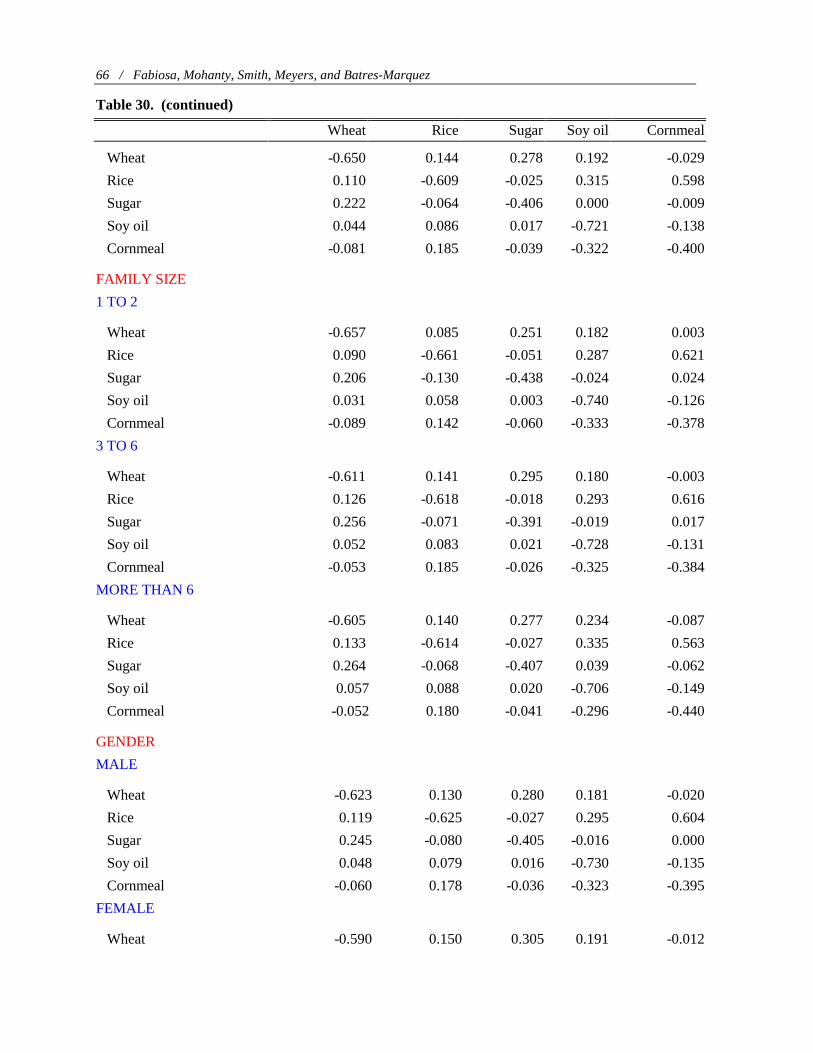
66 / Fabiosa, Mohanty, Smith, Meyers, and Batres-Marquez
Table 30. (continued)
Wheat Rice Sugar Soy oil Cornmeal
Wheat -0.650 0.144 0.278 0.192 -0.029
Rice 0.110 -0.609 -0.025 0.315 0.598
Sugar 0.222 -0.064 -0.406 0.000 -0.009
Soy oil 0.044 0.086 0.017 -0.721 -0.138
Cornmeal -0.081 0.185 -0.039 -0.322 -0.400
FAMILY SIZE
1 TO 2
Wheat -0.657 0.085 0.251 0.182 0.003
Rice 0.090 -0.661 -0.051 0.287 0.621
Sugar 0.206 -0.130 -0.438 -0.024 0.024
Soy oil 0.031 0.058 0.003 -0.740 -0.126
Cornmeal -0.089 0.142 -0.060 -0.333 -0.378
3 TO 6
Wheat -0.611 0.141 0.295 0.180 -0.003
Rice 0.126 -0.618 -0.018 0.293 0.616
Sugar 0.256 -0.071 -0.391 -0.019 0.017
Soy oil 0.052 0.083 0.021 -0.728 -0.131
Cornmeal -0.053 0.185 -0.026 -0.325 -0.384
MORE THAN 6
Wheat -0.605 0.140 0.277 0.234 -0.087
Rice 0.133 -0.614 -0.027 0.335 0.563
Sugar 0.264 -0.068 -0.407 0.039 -0.062
Soy oil 0.057 0.088 0.020 -0.706 -0.149
Cornmeal -0.052 0.180 -0.041 -0.296 -0.440
GENDER
MALE
Wheat -0.623 0.130 0.280 0.181 -0.020
Rice 0.119 -0.625 -0.027 0.295 0.604
Sugar 0.245 -0.080 -0.405 -0.016 0.000
Soy oil 0.048 0.079 0.016 -0.730 -0.135
Cornmeal -0.060 0.178 -0.036 -0.323 -0.395
FEMALE
Wheat -0.590 0.150 0.305 0.191 -0.012
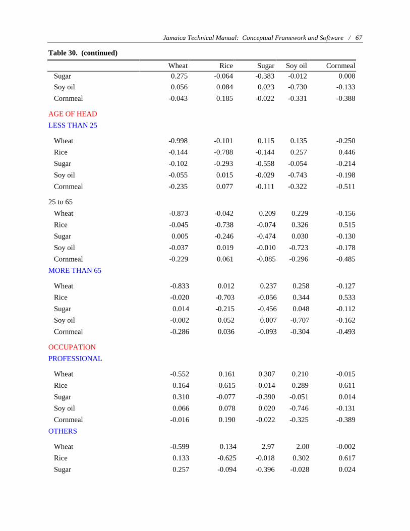
Jamaica Technical Manual: Conceptual Framework and Software / 67
Table 30. (continued)
Wheat Rice Sugar Soy oil Cornmeal
Sugar 0.275 -0.064 -0.383 -0.012 0.008
Soy oil 0.056 0.084 0.023 -0.730 -0.133
Cornmeal -0.043 0.185 -0.022 -0.331 -0.388
AGE OF HEAD
LESS THAN 25
Wheat -0.998 -0.101 0.115 0.135 -0.250
Rice -0.144 -0.788 -0.144 0.257 0.446
Sugar -0.102 -0.293 -0.558 -0.054 -0.214
Soy oil -0.055 0.015 -0.029 -0.743 -0.198
Cornmeal -0.235 0.077 -0.111 -0.322 -0.511
25 to 65
Wheat -0.873 -0.042 0.209 0.229 -0.156
Rice -0.045 -0.738 -0.074 0.326 0.515
Sugar 0.005 -0.246 -0.474 0.030 -0.130
Soy oil -0.037 0.019 -0.010 -0.723 -0.178
Cornmeal -0.229 0.061 -0.085 -0.296 -0.485
MORE THAN 65
Wheat -0.833 0.012 0.237 0.258 -0.127
Rice -0.020 -0.703 -0.056 0.344 0.533
Sugar 0.014 -0.215 -0.456 0.048 -0.112
Soy oil -0.002 0.052 0.007 -0.707 -0.162
Cornmeal -0.286 0.036 -0.093 -0.304 -0.493
OCCUPATION
PROFESSIONAL
Wheat -0.552 0.161 0.307 0.210 -0.015
Rice 0.164 -0.615 -0.014 0.289 0.611
Sugar 0.310 -0.077 -0.390 -0.051 0.014
Soy oil 0.066 0.078 0.020 -0.746 -0.131
Cornmeal -0.016 0.190 -0.022 -0.325 -0.389
OTHERS
Wheat -0.599 0.134 2.97 2.00 -0.002
Rice 0.133 -0.625 -0.018 0.302 0.617
Sugar 0.257 -0.094 -0.396 -0.028 0.024
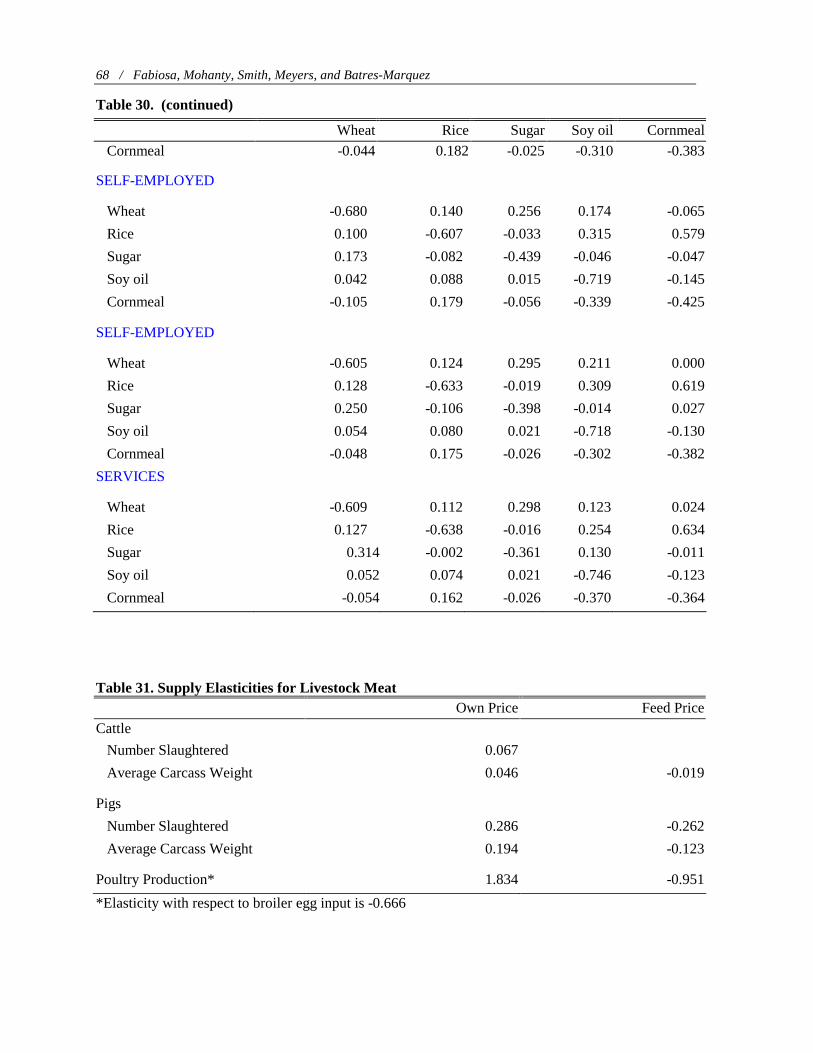
68 / Fabiosa, Mohanty, Smith, Meyers, and Batres-Marquez
Table 30. (continued)
Wheat Rice Sugar Soy oil Cornmeal
Cornmeal -0.044 0.182 -0.025 -0.310 -0.383
SELF-EMPLOYED
Wheat -0.680 0.140 0.256 0.174 -0.065
Rice 0.100 -0.607 -0.033 0.315 0.579
Sugar 0.173 -0.082 -0.439 -0.046 -0.047
Soy oil 0.042 0.088 0.015 -0.719 -0.145
Cornmeal -0.105 0.179 -0.056 -0.339 -0.425
SELF-EMPLOYED
Wheat -0.605 0.124 0.295 0.211 0.000
Rice 0.128 -0.633 -0.019 0.309 0.619
Sugar 0.250 -0.106 -0.398 -0.014 0.027
Soy oil 0.054 0.080 0.021 -0.718 -0.130
Cornmeal -0.048 0.175 -0.026 -0.302 -0.382
SERVICES
Wheat -0.609 0.112 0.298 0.123 0.024
Rice 0.127 -0.638 -0.016 0.254 0.634
Sugar 0.314 -0.002 -0.361 0.130 -0.011
Soy oil 0.052 0.074 0.021 -0.746 -0.123
Cornmeal -0.054 0.162 -0.026 -0.370 -0.364
Table 31. Supply Elasticities for Livestock Meat Own Price Feed Price
Cattle
Number Slaughtered 0.067
Average Carcass Weight 0.046 -0.019
Pigs
Number Slaughtered 0.286 -0.262
Average Carcass Weight 0.194 -0.123
Poultry Production* 1.834 -0.951
*Elasticity with respect to broiler egg input is -0.666
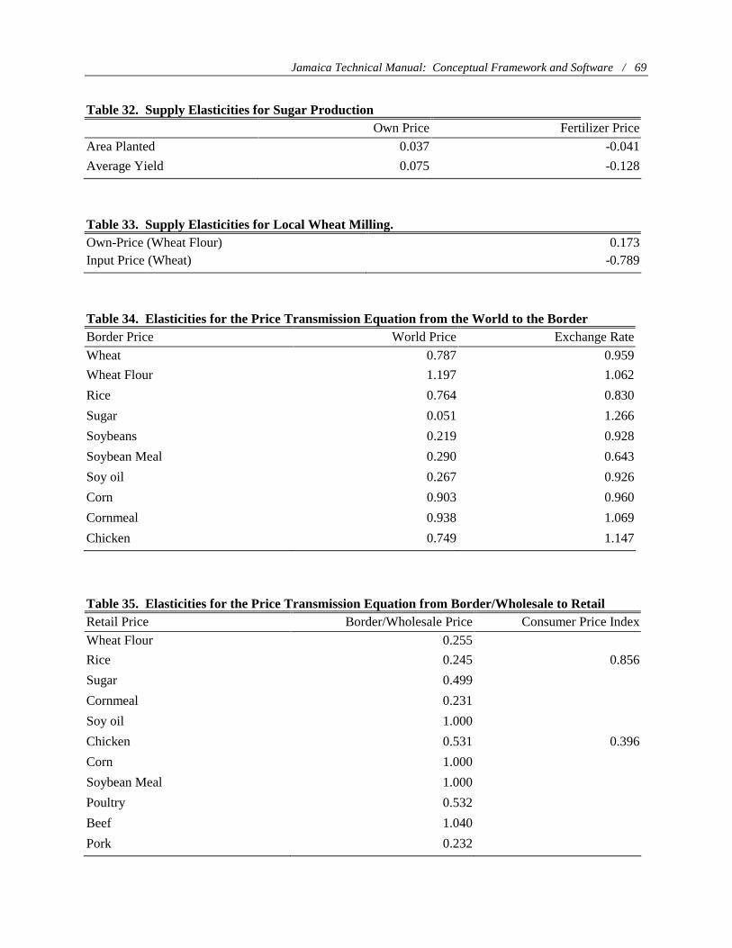
Jamaica Technical Manual: Conceptual Framework and Software / 69
Table 32. Supply Elasticities for Sugar Production
Own Price Fertilizer Price
Area Planted 0.037 -0.041
Average Yield 0.075 -0.128
Table 33. Supply Elasticities for Local Wheat Milling. Own-Price (Wheat Flour) 0.173 Input Price (Wheat) -0.789
Table 34. Elasticities for the Price Transmission Equation from the World to the Border Border Price World Price Exchange Rate
Wheat 0.787 0.959
Wheat Flour 1.197 1.062
Rice 0.764 0.830
Sugar 0.051 1.266
Soybeans 0.219 0.928
Soybean Meal 0.290 0.643
Soy oil 0.267 0.926
Corn 0.903 0.960
Cornmeal 0.938 1.069
Chicken 0.749 1.147
Table 35. Elasticities for the Price Transmission Equation from Border/Wholesale to Retail Retail Price Border/Wholesale Price Consumer Price Index
Wheat Flour 0.255
Rice 0.245 0.856
Sugar 0.499
Cornmeal 0.231
Soy oil 1.000
Chicken 0.531 0.396
Corn 1.000
Soybean Meal 1.000
Poultry 0.532
Beef 1.040
Pork 0.232

70 / Fabiosa, Mohanty, Smith, Meyers, and Batres-Marquez
Table 36. Elasticities for the Price Transmission Equation from Border to Wholesale Wholesale Price of Commodity Border Price Consumer Price Index
Wheat Flour 0.027 0.645
Chicken 0.260 0.600
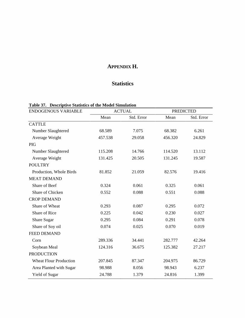
APPENDIX H.
Statistics
Table 37. Descriptive Statistics of the Model Simulation ENDOGENOUS VARIABLE ACTUAL PREDICTED
Mean Std. Error Mean Std. Error
CATTLE
Number Slaughtered 68.589 7.075 68.382 6.261
Average Weight 457.538 29.058 456.320 24.829
PIG
Number Slaughtered 115.208 14.766 114.520 13.112
Average Weight 131.425 20.505 131.245 19.587
POULTRY
Production, Whole Birds 81.852 21.059 82.576 19.416
MEAT DEMAND
Share of Beef 0.324 0.061 0.325 0.061
Share of Chicken 0.552 0.088 0.551 0.088
CROP DEMAND
Share of Wheat 0.293 0.087 0.295 0.072
Share of Rice 0.225 0.042 0.230 0.027
Share Sugar 0.295 0.084 0.291 0.078
Share of Soy oil 0.074 0.025 0.070 0.019
FEED DEMAND
Corn 289.336 34.441 282.777 42.264
Soybean Meal 124.316 36.675 125.382 27.217
PRODUCTION
Wheat Flour Production 207.845 87.347 204.975 86.729
Area Planted with Sugar 98.988 8.056 98.943 6.237
Yield of Sugar 24.788 1.379 24.816 1.399
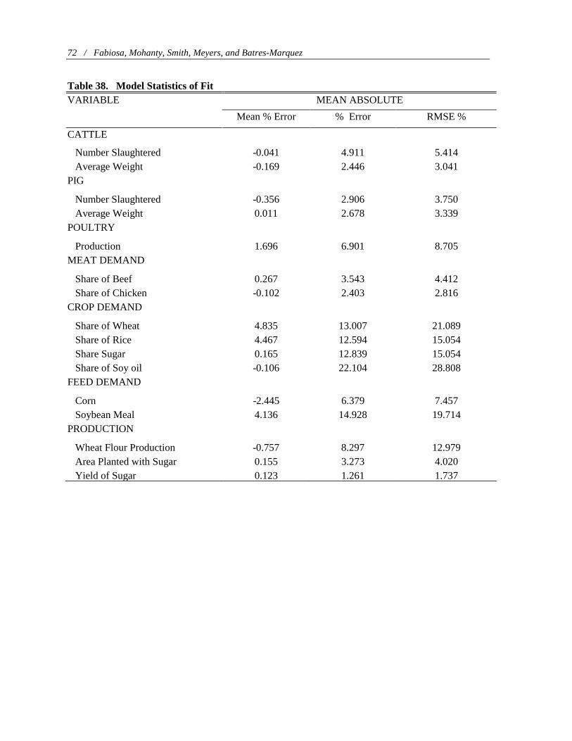
72 / Fabiosa, Mohanty, Smith, Meyers, and Batres-Marquez
Table 38. Model Statistics of Fit VARIABLE MEAN ABSOLUTE
Mean % Error % Error RMSE %
CATTLE
Number Slaughtered -0.041 4.911 5.414 Average Weight -0.169 2.446 3.041 PIG
Number Slaughtered -0.356 2.906 3.750 Average Weight 0.011 2.678 3.339 POULTRY
Production 1.696 6.901 8.705 MEAT DEMAND
Share of Beef 0.267 3.543 4.412 Share of Chicken -0.102 2.403 2.816 CROP DEMAND
Share of Wheat 4.835 13.007 21.089 Share of Rice 4.467 12.594 15.054 Share Sugar 0.165 12.839 15.054 Share of Soy oil -0.106 22.104 28.808 FEED DEMAND
Corn -2.445 6.379 7.457 Soybean Meal 4.136 14.928 19.714 PRODUCTION
Wheat Flour Production -0.757 8.297 12.979 Area Planted with Sugar 0.155 3.273 4.020 Yield of Sugar 0.123 1.261 1.737
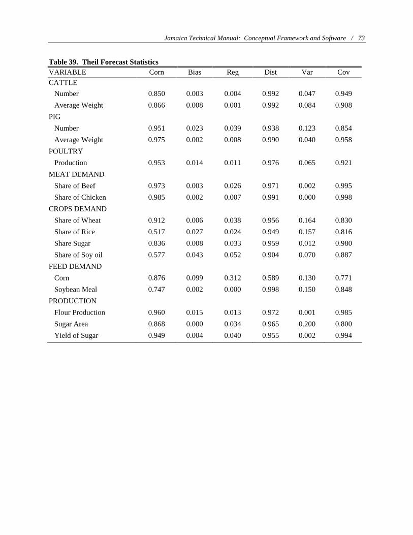
Jamaica Technical Manual: Conceptual Framework and Software / 73
Table 39. Theil Forecast Statistics VARIABLE Corn Bias Reg Dist Var Cov
CATTLE
Number 0.850 0.003 0.004 0.992 0.047 0.949
Average Weight 0.866 0.008 0.001 0.992 0.084 0.908
PIG
Number 0.951 0.023 0.039 0.938 0.123 0.854
Average Weight 0.975 0.002 0.008 0.990 0.040 0.958
POULTRY
Production 0.953 0.014 0.011 0.976 0.065 0.921
MEAT DEMAND
Share of Beef 0.973 0.003 0.026 0.971 0.002 0.995
Share of Chicken 0.985 0.002 0.007 0.991 0.000 0.998
CROPS DEMAND
Share of Wheat 0.912 0.006 0.038 0.956 0.164 0.830
Share of Rice 0.517 0.027 0.024 0.949 0.157 0.816
Share Sugar 0.836 0.008 0.033 0.959 0.012 0.980
Share of Soy oil 0.577 0.043 0.052 0.904 0.070 0.887
FEED DEMAND
Corn 0.876 0.099 0.312 0.589 0.130 0.771
Soybean Meal 0.747 0.002 0.000 0.998 0.150 0.848
PRODUCTION
Flour Production 0.960 0.015 0.013 0.972 0.001 0.985
Sugar Area 0.868 0.000 0.034 0.965 0.200 0.800
Yield of Sugar 0.949 0.004 0.040 0.955 0.002 0.994

REFERENCES
Bank of Jamaica. Statistical Digest (various years). Research and Programming Division. Bank of Jamaica. Kingston.
Devadoss, S., Michael Helmar, and William H. Meyers. The World Wheat Trade Model: Specification,
Estimation ,and Validation. Technical Report 90-TR14. Ames: Center for Agricultural and Rural Development, Iowa State University, 1990.
Helmar, Michael, S. Devadoss, and William H. Meyers. The World Feed-Grains Trade Model:
Specification, Estimation, and Validation. Technical Report 91-TR18. Ames: Center for Agricultural and Rural Development, Iowa State University, 1991.
Helmar, Michael D., V. Premakumar, Karen Oerter, John Kruse, Darnell B. Smith, and William H.
Meyers. Impacts of the Uruguay Round on Agricultural Commodity Markets. GATT Research Paper 94-GATT 21. Ames: Center for Agricultural and Rural Development, Iowa State University, 1994.
Meyers, William H., S. Devadoss, and Michael Helmar. The World Soybean Trade Model.
Specification, Estimation, and Validation. Technical Report 91-TR23. Ames: Center for Agricultural and Rural Development, Iowa State University, 1991.
Planning Institute of Jamaica. Economic and Social Survey Jamaica (various years). PIOJ, Barbados
Ave, Kingston. Premakumar, V., Karen Oerter, Darnell B. Smith, and William H. Meyers. Uruguay Round Agreement
on Agriculture: Summary of Commitments from Selected Country Schedules. GATT Research Paper 94-GATT 23. Ames: Center for Agricultural and Rural Development, Iowa State University, 1994.
Statistical Institute of Jamaica. Consumer Price Index (various years). STATIN, Swallowfield Road,
Kingston. Statistical Institute of Jamaica. External Trade Part I and Part II (various years). STATIN,
Swallowfield Road, Kingston. Statistical Institute of Jamaica. Production Statistics (various years). STATIN, Swallowfield Road,
Kingston. Statistical Institute of Jamaica. Statistical Yearbook of Jamaica (various years). STATIN, Swallowfield
Road, Kingston.

76 / Fabiosa, Mohanty, Smith, Meyers, and Batres-Marquez