The Fountain That Math Builtmath.tongji.edu.cn/model/docs/amccauleymcm2002a.pdf · 2018-03-08 · Our task is to design an algorithm that controls the ﬂow rate of the fountain,

The Fountain That Math Built 221

The Fountain That Math Built

Alex McCauleyJosh MichenerJadrian MilesNorth Carolina School of Science and MathematicsDurham, NC

Advisor: Daniel J. Teague

IntroductionWe are presented with a fountain in the center of a large plaza, which we

wish to be as attractive as possible but not to splash passersby on windy days.Our task is to design an algorithm that controls the flow rate of the fountain,given input from a nearby anemometer.

During calm, the fountain sprays out water at a steady rate. When thewind picks up, the flow should be attenuated so as to keep the water within thefountain’s pool; in this way, we strike a balance between esthetics and comfort.

We consider the water stream from the fountain as a collection of different-sized droplets that initially leave the fountain nozzle in the shape of a perfectcylinder. This cylinder is broken into its component droplets by the wind, withsmaller droplets carried farther. In the reference frame of the air, a droplet ismoving through stationary air and experiencing a drag force as a result; sincethe air is moving with a constant velocity relative to the fountain, the force onthe droplet is the same in either frame of reference.

Modeling this interaction as laminar flow, we arrive at equations for thedrag forces. From these equations, we derive the acceleration of the droplet,which we integrate to find the equations of motion for the droplet. These allowus to find the time when the droplet hits the ground and—assuming that itlands at the very edge of the pool—the time when it reaches its maximumrange from the horizontal position equation. Equating these and solving theinitial flow rate, we arrive at an equation for the optimal flow rate at a givenconstant wind speed. Since the wind speeds are not constant, the algorithmmust make its best prediction of wind speed and use current and previous windspeed measurements to damp out transient variations.

The UMAP Journal 23 (3) (2002) 221–234. c©Copyright 2002 by COMAP, Inc. All rights reserved.Permission to make digital or hard copies of part or all of this work for personal or classroom useis granted without fee provided that copies are not made or distributed for profit or commercialadvantage and that copies bear this notice. Abstracting with credit is permitted, but copyrightsfor components of this work owned by others than COMAP must be honored. To copy otherwise,to republish, to post on servers, or to redistribute to lists requires prior permission from COMAP.

222 The UMAP Journal 23.3 (2002)

Our final solution is an algorithm that takes as its input a series of windspeed measurements and determines in real time the optimal flow rate to max-imize the attractiveness of the fountain while avoiding splashing passersbyexcessively. Each iteration, it adds an inputted wind speed to a buffer of pre-vious measurements. If the wind speed is increasing sufficiently, the last 0.5 sof the buffer are considered; otherwise, the last 1 s is. The algorithm computesa weighted average of these wind speeds, weighting the most recent valueslightly more than the oldest value considered. It uses this weighted veloc-ity average in the equation that predicts the optimal flow rate under constantwind. The result is the optimal flow rate under variable wind, knowing onlycurrent and previous wind speeds.

A list of relevant variables, constants, and parameters is in Table 1.

Table 1.

Relevant constants, variables, and parameters.

Physical constants Description Value

ηa Viscosity of air 1.849 × 10−5 kg/m·s[Lide 1999]

ρw Density of water 1000 kg/m3

ρa Density of air 1.2 × 10−6 kg/m3

Situational constants Units

A Cross-sectional area of fountain nozzle m2

fmax Maximum flow rate of fountain’s pump m3/sRp Radius of fountain pool mr Radius of smallest uncomfortable water m

dropletdt Sampling interval of anemometer sk k = 9ηa/2ρwr2

Situational variables

va Instantaneous wind speed m/sf Instantaneous flow rate of water m3/s

from the fountainn n = g/k + f/A m/s

Dynamic variables

x(t), y(t) Droplet’s horizontal and vertical positions mvx(t), vy(t) Droplet’s horizontal and vertical speeds m/sax(t), ay(t) Droplet’s horizontal and vertical accelerations m/s2

Situational parameters

τd Default sample wind velocity buffer time sτi Buffer time for quickly increasing sample s

wind velocitiesK Weight constant dimensionless


Assumptions• Passersby find a higher spray more attractive.

• Avoiding discomfort is more important to passersby than the attractivenessof the fountain.

• The water stream can be considered a collection of spherical droplets, eachof which has no initial horizontal component of velocity.

• Every possible size of sufficiently small water droplet is represented in thewater stream in significant numbers.

• Water droplets remain spherical.

• The interaction between the water droplets and wind can be described asnon-turbulent, or “laminar,” flow.

• There exists a minimum uncomfortable water droplet size; passersby find itacceptable to be hit by any droplets below this size but by none above.

• When the wind enters the plaza, its velocity is entirely horizontal.

• The wind speed is the same throughout the plaza at any given time.

• The pool and the area around it are radially symmetric, so there is no pre-ferred radial direction.

• We can neglect any buoyant force on the water due to the air, since the errorintroduced by this approximation is equal to the ratio of densities of thefluids involved, on the order of 10−3, which is negligible.

• The anemometer reports wind speeds at discrete time intervals dt.

Analysis of the ProblemFor a water stream viewed as a collection of small water droplets blown

from a core stream, the interaction between the droplets and the air movingpast them can best be described in the inertial reference frame of the movingair. In this frame, the air is stationary while the droplet moves horizontallythrough the air with a speed equal to the relative speed of the droplet andwind, vr = va − vx. In the vertical direction, vr = vy , since the wind blowshorizontally.

In the air’s frame of reference, the water droplet experiences a drag forceopposing vr. Assuming that the air moves at a constant velocity, this forceis the same in both frames of reference. In the frame of the fountain, then,the droplet is being blown in the direction of the wind. The smaller waterdroplets are carried farther, so we need only consider the motion of the smallest


uncomfortable water droplets, knowing that bigger droplets do not travel asfar.

The water droplet initially has a vertical velocity vy(0) that is directly relatedto the flow rate of water through the nozzle of the fountain. This initial verticalvelocity component can be controlled by changing the flow rate. The droplet’smotion causes vertical air resistance, slowing the droplet and affecting howlong (tw) the droplet is in the air.

Since the vertical and horizontal components of a water droplet’s motionare independent, tw is determined solely by the vertical motion. Knowingthis time allows us to find the horizontal distance traveled, which we wish toconstrain to the radius of the pool.

When the wind is variable, however, we cannot determine exactly the idealflow rate for any given time. We must instead act on the current reading butalso rely on previous measurements of wind speed in order to restrain themodel from reacting too severely to wind fluctuations. We need to react fast toincreases in wind speed, since they result in splashing which is weighted moreheavily.

Design of the ModelFor our initial model, we assume that va is constant for time intervals on

the order of tw, so that any given droplet experiences a constant wind speed.We model the water stream as a collection of droplets that are initially co-

hesive but are carried away at varying velocities by the wind. The distancesthat they travel depend on the wind speed va and the initial vertical velocity ofthe water stream through the nozzle, vy(0). Since the amount of water flowingthrough the nozzle per unit time is f = vy(0)A, we have vy(0) = f/A. Thedynamics of the system, then, is fully determined by f and va. First, we findthe equations of motion for the droplet.

Equations of Motion for a DropletFor laminar flow, a spherical particle of radius r traveling with speed v

through a fluid medium of viscosity η experiences a drag force FD such that

FD = (6πηr)v [Winters 2002].

Since a spherical water droplet has a mass given by

m = ρw

(43 πr3

),

the acceleration felt by the droplet is given by Newton’s Second Law as thetotal force over mass. Since there are no other forces acting in the horizontal


direction, the horizontal acceleration ax is given by:

ax(t) =d2x

dt2=

(9ηa

2ρwr2

)vr = k(va − vx), (1)

where k = 9ηa/2ρwr2.The droplet experiences both air drag and gravity in the vertical direction,

so the vertical acceleration is

ay(t) = −[(

9ηa

2ρwr2

)vy + g

]= −k

(vy +

g

k

).

With constant va, we use separation of variables and integrate to find vx(t) andvy(t), using the facts that vx(0) = 0 and vy(0) = f/A. The results are

vx(t) = va

(1 − e−kt

), vy(t) = ne−kt − g

k,

where n = g/k + f/A.Integrating again, and using x(0) = y(0) = 0, we have

vx(t) =va

k

(kt + e−kt − 1

), vy(t) =

1k

n(1 − e−kt

)− gt.

Determining the Flow RateBecause f is the only parameter that the algorithm modifies, we wish to find

the flow rate that would restrict the smallest uncomfortable water droplets toranges within Rp, so that they would land in the fountain’s pool.

After a time tw, the droplet has fallen back to the ground. Thus, y(tw) = 0.This equation is too difficult to solve exactly, so we use the series expansionfor e−kt and truncate after the quadratic term: e−kt ≈ 1 − x + x2/2. Solvingy(tw) = 0, we find

tw ≈ 2k

(1 − g

nk

).

We know that the maximum horizontal distance x(tw) must be less than orequal to Rp, with equality holding for the smallest uncomfortable droplet. Forthat case, using the same expansion for e−kt as above,

Rp = x(tw) ≈ va

k

(ktw − 1 + 1 − ktw +

(ktw)2

2

)=

vak

2t2w.

Solving for tw and equating it to the earlier expression for tw, we get√2Rp

vak= tw =

2k

(1 − g

nk

).


Recalling that in this equality only n is a function of f , we substitute for n andsolve for f . The result is

f(va) =Ag√

2vak

Rp− k

. (2)

As va → kRp/2, this equation becomes singular (see Figure 2). At lower valuesof va, it gives a negative flow rate. These wind speeds are very small; at suchspeeds, the droplets would not be deflected significantly by the wind. Since(2) assumes that the flow rate can be made arbitrarily high, it is unrealistic andinvalid in application. To make the model more reasonable, we modify (2) toinclude the maximum flow rate achievable by the pump, fmax:

F (va) =

min

Ag√2vak

Rp− k

, fmax

, va > kRp/2;

fmax, va ≥ kRp/2.

(3)

An algorithm can use the given constants and a suitable minimal dropletsize to determine the appropriate flow rate for a measured va. However, (3)assumes that the wind speed is constant over the time scale tw for any givendroplet. A more realistic model must take into account variable wind speed.

Variable Wind SpeedWhen wind speed varies with time, the physical reasoning used above be-

comes invalid, since the relative velocity of the reference frames is no longer con-stant. Mathematically, this is manifested in the equation for velocity-dependenthorizontal acceleration; integrating is now not so simple, and we must resort tonumerical means to find the equations of motion. Additionally, the algorithmcan rely only on past and present wind data to find the appropriate flow rate.Our model needs to incorporate these wind data to make a reasonable predic-tion of the wind’s velocity over the next tw and determine an appropriate flowrate using (3).

A gust is defined to be a sudden wind speed increase on the order 5 m/sthat lasts for no more than 20 s; a squall is a similarly sudden wind speedincrease that lasts longer [Weather Glossary 2002]. Our model should accountfor gusts and squalls, as well as for “reverse” gusts and squalls, in which thewind speed suddenly decreases. Since wind speeds can change drastically andunpredictably over the flight time of a droplet, our model will behave badlyat times and there is no way to completely avoid this—only to minimize itseffects.


The model’s reaction to wind speed is not fully manifested until the dropletlands, after a time tw (approximately 2 s). By the time our model has reacted to agust or reverse gust, therefore, the wind speed has stopped changing. Withoutsome type of buffer, in a gust our model would react by suddenly droppingflow rate as the wind peaked and then increasing it again as the wind decreased;the fountain would virtually cut off for the duration of any gust, which wouldrelease less water and thus seem very unattractive to passersby. Additionally,the water released just before the onset of the gust would be airborne as thewind speed picked up, splashing passersby regardless of any reaction by ourmodel.

We exhibit an algorithm for analyzing wind data that makes use of (3).Because velocity now varies within times on the order of tw, we do not want todirectly input the current wind speed but rather a buffered value, so that themodel does not react too sharply to transient wind changes. The model shouldreact more quickly to sudden increases in wind than to decreases, becauseincreases cause splashing, which we weight more heavily than attractiveness.

The model, therefore, has two separate velocity buffer times: one, τd, thedefault, and another, τi, for when the wind increases drastically. We also weightmore-recent values in the buffer more heavily, since we want the model to reactpromptly to wind speed changes but not to overreact. We weight each valuein the velocity buffer with a constant value K plus a weight proportional toits age: Less-recent velocities are considered but given less weight than morerecent ones. The weight of the oldest value in the buffer is K and that of themost recent is K+1, with a linear increase between the two. With the constraintthat the weights are normalized (i.e., they sum to 1), the equation for the ithweight factor is

wi =

(K +

i

τ − dt

)dt(

K +12

)τ

.

The speeds are multiplied by their respective normalized weights and summed.This sum, v∗, is then used in (3) to find the appropriate flow rate for the fountainat a given time. We use τi rather than τd when the wind speed increases suf-ficiently over a recent interval, but not when it increases slightly or fluctuatesrapidly. We switch from τd to τi whenever the wind speed increases over twosuccessive 0.2 s intervals and by a total of at least 1 m/s over the entire 0.4 sinterval.

Our algorithm follows the flow chart in Figure 1 in computing the currentflow rate

We wrote a C++ program to compute this algorithm, the code for which isincluded in an appendix. [EDITOR’S NOTE: We omit the code.]


Figure 1. Flow chart for computing flow rate with variable wind speed.

Testing and Sensitivity Analysis

Sensitivity of Flow EquationIn our equation for flow rate, two variables can change: minimal droplet size

and wind speed. While the minimal droplet size will not change dynamically,its value is a subjective choice that must be made by the owner of the fountain.The wind speed, however, will change dynamically throughout the problem,and the purpose of our model is to react to these changes.

We examined (3) for varying minimal drop sizes (Figure 2) and wind speeds(Figure 3). We used a fountain with nozzle radius 1 cm, maximum flow rate7.5 L/s, and pool radius 1.2 m. (This maximum flow rate is chosen for illustra-tive purposes and is not reasonable for such a small fountain.)

Figure 2. Graphs of flow rate f vs. wind speed va for several values of radius r of smallestuncomfortable droplet.


At any wind speed, as the acceptable droplet radius decreases, the flow rateo decreases. At higher wind speeds, this difference is less pronounced; but atlower speeds, acceptable size has a significant impact on the flow rate. At verylow wind speeds, the fountain cannot shoot the droplets high enough to allowthe wind to carry them outside the pool, regardless of drop size. Our cutoff,fmax, reflects that the fountain pump cannot generate the extreme flow neededto get the droplets to the edge of the pool in these conditions.

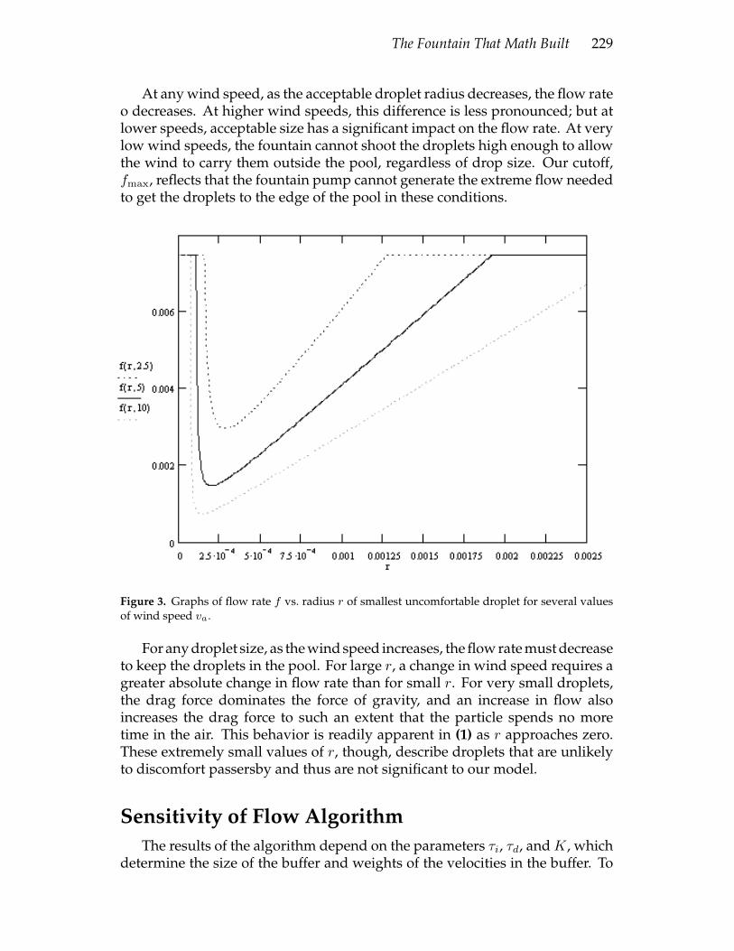
Figure 3. Graphs of flow rate f vs. radius r of smallest uncomfortable droplet for several valuesof wind speed va.

For any droplet size, as the wind speed increases, the flow rate must decreaseto keep the droplets in the pool. For large r, a change in wind speed requires agreater absolute change in flow rate than for small r. For very small droplets,the drag force dominates the force of gravity, and an increase in flow alsoincreases the drag force to such an extent that the particle spends no moretime in the air. This behavior is readily apparent in (1) as r approaches zero.These extremely small values of r, though, describe droplets that are unlikelyto discomfort passersby and thus are not significant to our model.

Sensitivity of Flow AlgorithmThe results of the algorithm depend on the parameters τi, τd, and K, which

determine the size of the buffer and weights of the velocities in the buffer. To


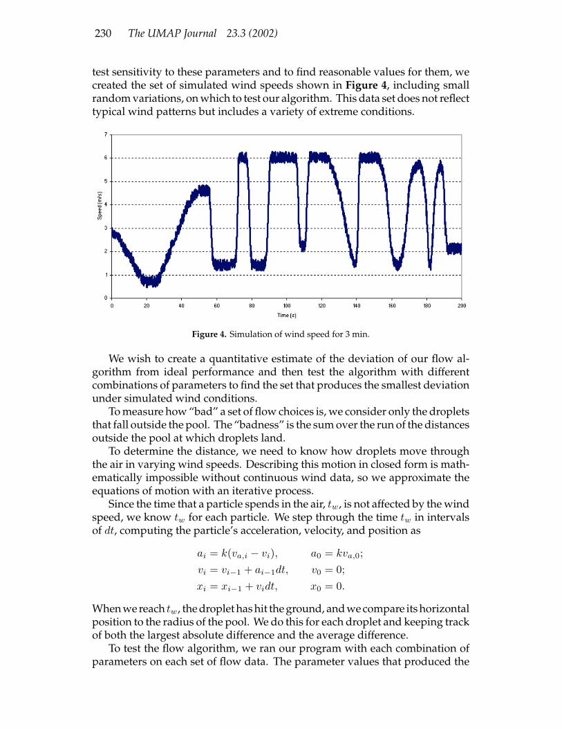
test sensitivity to these parameters and to find reasonable values for them, wecreated the set of simulated wind speeds shown in Figure 4, including smallrandom variations, on which to test our algorithm. This data set does not reflecttypical wind patterns but includes a variety of extreme conditions.

Figure 4. Simulation of wind speed for 3 min.

We wish to create a quantitative estimate of the deviation of our flow al-gorithm from ideal performance and then test the algorithm with differentcombinations of parameters to find the set that produces the smallest deviationunder simulated wind conditions.

To measure how “bad” a set of flow choices is, we consider only the dropletsthat fall outside the pool. The “badness” is the sum over the run of the distancesoutside the pool at which droplets land.

To determine the distance, we need to know how droplets move throughthe air in varying wind speeds. Describing this motion in closed form is math-ematically impossible without continuous wind data, so we approximate theequations of motion with an iterative process.

Since the time that a particle spends in the air, tw, is not affected by the windspeed, we know tw for each particle. We step through the time tw in intervalsof dt, computing the particle’s acceleration, velocity, and position as

ai = k(va,i − vi), a0 = kva,0;vi = vi−1 + ai−1dt, v0 = 0;xi = xi−1 + vidt, x0 = 0.

When we reach tw, the droplet has hit the ground, and we compare its horizontalposition to the radius of the pool. We do this for each droplet and keeping trackof both the largest absolute difference and the average difference.

To test the flow algorithm, we ran our program with each combination ofparameters on each set of flow data. The parameter values that produced the


least deviation were τi = 0.5, τd = 1, and K = 10. These values imply thatonly fairly recent wind speed measurements should be held in the buffer, withmost recent velocity having a weight of (K + 1)/K = 1.1 relative to the oldest.Lowering K beyond this value increases the deviation from the ideal, whileincreasing it further makes no difference. Similarly, increasing τi or τd increasesthe deviation, because the algorithm cannot respond quickly to changes in windspeed. Decreasing τi below 0.5 makes no difference, while decreasing τd wouldmake the model too sensitive to short fluctuations in wind speed.

Figure 5. Range of droplets over the simulation overlaid with scaled wind speeds.

Justification

Validity of the Laminar Flow AssumptionOur model is based on a drag force proportional to vr, which is not nec-

essarily correct. For higher speeds or large droplet sizes, the drag becomesproportional to v2

r . We thus need to determine whether reasonable physicalscenarios allow us to model the drag force as proportional to and not v2

r .For a sphere of radius r moving through the air with speed vr, the Reynolds

number R is defined to beR =

2ρavr

ηar [Winters 2002].

When R < 103, there is little turbulence and laminar flow dominates, soair resistance is roughly proportional to vr. If R > 103, the flow is turbulentand the drag force is proportional to v2

r [Winters 2002]. Using a physicallyreasonable relative speed of 4.5 m/s (corresponding to a wind speed of roughly10 mph), we obtain R = (5.8× 105)r, which gives predominantly laminar flowwhen r < 1.7 mm. Because water droplets of diameter greater than 3 mm areuncomfortable, these provide an upper limit on the droplet sizes to consider.


Because these smaller droplets bound the larger droplets in how far they gofrom the fountain (see below), all of our analysis is concerned with dropletswhose sizes are within the allowed range for laminar flow.

Bounding the Droplet RangeFor either laminar or turbulent flow, the acceleration due to drag scales with

as F/m ∝ r−n, where 1 ≤ n ≤ 2. Larger droplets therefore experience a lowerhorizontal acceleration due to drag, while acceleration in the vertical directionis dominated by gravity (k < 0.1g); so the time that a particle spends in the airis roughly the same for droplets of varying radius. The heavier droplets haveless horizontal acceleration, so they travel a shorter horizontal distance in thesame amount of time than smaller droplets. The ranges are, therefore, shorterfor larger droplets, so we can bound all uncomfortably-sized droplets by therange of the smallest such droplet.

Initial Shape of the Water StreamWe assume that the water coming out of the fountain nozzle has no initial

horizontal velocity; that is, the stream is a perfect cylinder with the same radiusas the nozzle. In fact, the stream is closer to the shape of a steep cone and thedroplets have some horizontal velocity. In the absence of wind, this assumptionhas a significant impact on where the droplets land, since without wind thealgorithm predicts a horizontal range of zero. However, in these cases, theflow rate is bounded by fmax regardless of initial velocity, so the natural spreadof the fountain is irrelevant. In higher wind, the initial horizontal velocityis quickly dominated by the acceleration due to the wind and thus makes anegligible contribution to the total range.

Exclusively Horizontal WindWe assume that the wind is exclusively horizontal. Since the anemometer

measures only horizontal wind speed, that is the only component that we canconsider in our model. Additionally, the buildings around the plaza wouldtend to act as a wind tunnel and channel the wind horizontally.

Quadratic Approximation of e−kt

Because the series for e−kt is alternating, the error from truncating after thesecond term is no greater than the third term, which is (kt)3/6. The relative erroris (kt)3/e−kt ≈ 0.001 for reasonable values of k and t, so our approximationintroduces very little error.


ConclusionsOur final solution is an algorithm that takes as its input a series of wind

speed measurements and determines in real-time the optimal flow rate to max-imize the attractiveness of the fountain while avoiding splashing passersbyexcessively. It takes an inputted wind speed and adds it to a buffer of previousmeasurements. If the wind speed is increasing sufficiently, the last 0.5 s of thebuffer are considered; otherwise, the last 1 s is. The algorithm computes aweighted average of these wind speeds, weighting the most recent value 10%more heavily than the oldest value considered. It then takes this weighted aver-age and uses it in the equation that predicts the optimal flow rate under constantwind. The result is the optimal flow rate under variable wind, knowing onlycurrent and previous wind speeds.

Strengths and Weaknesses

Strengths• Given reasonable values for the characteristics of the fountain and for wind

behavior, our model returns values that satisfy the goal of maintaining anattractive fountain without excessively splashing passersby.

• The model can compute optimal flow rates in real time. Running one cycleof the algorithm takes a time on the order of 0001 s, so the fountain’s pumpcould be adjusted as fast as physically possible.

• The constants that determine the behavior of the algorithm, τd, τi, and K,are not arbitrary but instead perform best under simulation.

• Our algorithm is very robust; it works well under extreme conditions andcan be readily modified for different situations or fountains.

Weaknesses• A primary assumptions is that the droplets coming from the fountain nozzle

have no horizontal velocity. In reality, the nozzle sprays a cone of water,rather than a perfect cylinder; but this difference does not have a significantimpact on the results.

• Another important assumption is laminar flow. The water droplets are of asize to experience a combination of laminar and turbulent flow, but describ-ing such a combination of regimes is mathematically difficult and is knownonly through experimentation. A more rigorous representation of the dragforce would increase the accuracy of our simulation, but doing so would


markedly increase the complexity of the algorithm and thus make real-timecomputation more difficult.

• We have ignored the abundances of droplet sizes in considering discom-fort. If one droplet would spray passersby, we assume that enough dropletswould spray passersby to make them uncomfortable. In fact, it is only sig-nificant numbers of droplets that discomfort passersby; but we do not knowhow many droplets would be released nor how many would be needed tobe discomforting.

ReferencesGoldstein, S., ed. 1965. Modern Developments in Fluid Dynamics. Vol. 2. New

York: Dover.

Hughes, W.F., and J.A. Brighton. 1967. Fluid Dynamics. New York: McGraw-Hill.

Lide, David R., ed. 1999. CRC Handbook of Chemistry and Physics. 80th ed. BocaRaton, FL: CRC Press.

Winters, L. 2002. Theory of velocity dependent drag forces. http://courses.ncssm.edu/ph220/labs/vlab1/theory.pdf . Accessed February 2002.

Weather Glossary. 2002. http://www.weather.com/glossary/ . AccessedFebruary 2002.

Documents

The Fountain That Math Builtmath.tongji.edu.cn/model/docs/amccauleymcm2002a.pdf · 2018-03-08 · Our task is to design an algorithm that controls the ﬂow rate of the fountain,