The Generation of Response Curves from Laboratory Tracer

SGP-TR-94

The Generation of Response Curves from Laboratory Tracer Flow

Experiments

J. Flint Pulskamp

December 1985

Financial support was provided through the Stanford Geothermal Program under Department of Energy Contract

No. DE-AT03-80SF11459 and by the Department of Petroleum Engineering, Stanford University

Stanford Geothermal Program Interdisciplinary Research in

Engineering and Earth Sciences STANFORD UNIVERSITY

Stanford, California

ABSTRACT

In order to interpret tracer tests in fractured reservoirs, mathematical models have

been used. However since model fitting is only an indirect process, it is necessary to

examine the applicability of the model by comparing it to closely controlled laboratory

flow experiments. In this way, the reliability and accuracy of the model can be evaluat-

ed and its functional limits can be defined. This study set out to collect data which

could be used as a basis to test the validity of mathematical models for tracer flow in

fractures, and in particular, models developed recently at Stanford. Laboratory experi-

ments were performed by flowing a potassium iodide (KI) tracer through various frac-

tured consolidated cores and then observing the response curves by measuring the

tracer ion concentration of the effluent over time. The response curves can be

analyzed by the models to estimate formation parameters such as fracture width in this

case.. By comparing the values of fracture width generated by the computer model to

that measured on the actual core, the model’s accuracy can be gauged. The original

experimental apparatus did not allow for a sufficient number of measurements to define

the response curves, however, the experimental limitations were defined and a practical

solution was outlined.

Table of Contents

Abstract ................................................................................................................................................ i

... List of Figures .................................................................................................................................... 111

List of Tables ..................................................................................................................................... iv

Section 1: Introduction .................................................................................................................. 1

Section 2: Literature Review ....................................................................................................... 3

Section 3: Experimental Apparatus ........................................................................................... 5

Section 4: Experimental Procedure ........................................................................................... 6

Running the Tracer ............................................................................................................ 6

Measuring the Tracer ........................................................................................................ 8

Section 5: Discussion of Results ............................................................................................... 11

Section 6: Conclusions .................................................................................................................. 20

Section 7: References .................................................................................................................... 21

Section 8: Appendix ....................................................................................................................... 23

.. -11-

List of Figures

FIGURE 1:

FIGURE 2:

FIGURE 3:

FIGURE 4:

FIGURE 5:

FIGURE 6:

FIGURE 7:

FIGURE 8:

Experimental Setup ................................................................................................

Schematic of Experimental Apparatus ............................................................

Run #3 ........................................................................................................................

Run #4 ........................................................................................................................

Run #5 ........................................................................................................................

Run #6 ........................................................................................................................

Run #8 ........................................................................................................................

Run #9 ........................................................................................................................

FIGURE 9: Run #10 ......................................................................................................................

6

7

16

16

17

17

18

18

19

... -111-

List of Tables

TABLE 1: Run #3 ........................................................................................................................... 14

TABLE 2: Run #4.5. 6 ................................................................................................................... 14

TABLE 3: Run #7 .......................................................................................................................... 15

TABLE 4: Run #8, 9 ....................................................................................................................... 15

TABLES: Run#lO ........................................................................................................................ 15

-iV-

-1-

SECTION 1: INTRODUCTION

In order to predict and understand the mechanisms of fluid flow in reservoirs,

characteristics of the formation and fluid must be defined. Formation charcteristics can

be determined directly by analyzing actual well core samples, although indirect

methods are more often used. Well tests and tracer tests are two such indirect methods,

and are by far the most common. Reservoir parameters which depend on both fluid

and formation characteristics, such as dispersion, diffusion, etc., are determined by

developing flow models to help predict the influence these parameters have on the

mechanisms of fluid flow. The more clearly defined the influences of these parame-

ters, the more accurately the behavior of the reservoir can be estimated using the

model. Since these parameters depend on fluid and formation characteristics, they be-

come difficult to measure. For this reason, when these parameters are incorporated

into models, it becomes very diffficult to verify the model’s accuracy. But one way to

examine the applicability of the model is to run experimental tracer tests in the labora-

tory and then compare the estimates of the parameter values with those that can be

measured directly on the laboratory core.

The model considered in this work is a two dimensional computer model

developed by Walkup (1984) to represent the flow of tracer in a fractured reservoir.

The objective of Walkup’s model was to be able to estimate fracture aperture by com-

paring the model results to tracer test measurements in a fractured reservoir. This

model involved six dimensionless variables, of which five are made up of combina-

tions of eight physical flow parameters. The sixth variable, dimensionless distance, is

of greatest interest because it contains only the two parameters fracture half width and

core length, both of which can be measured directly on a core. The measurement of

this parameter (fracture width) is the basis by which this model can be verified and is

the objective of this research.

- 2 -

This objective can be divided into 3 facets: (1) to devise an experimental method

by which a tracer flow test can be accurately simulated in a laboratory, (2) to devise a

method to create and measure "fractures" of different widths in the core, and (3) to

measure the tracer concentrations of the effluent.

- 3 -

SECTION 2: LITERATURE REVIEW

Laboratory work on tracer flow in fractures has been performed as a means to

understand the flow mechanisms in tracer tests. These principles have been incorporat-

ed into mathematical models to simulate flow in a fracture. The models have been ap-

plied to actual field test data, but their accuracy has not been verified by laboratory

controlled tracer flow experiments. A series of computer models to represent tracer

flow in fractures have been developed at Stanford University during the past five years

and only limited attempts have been made to test their accuracy.

Because the flow mechanisms in geothermal reservoirs are affected by the highly

fractured nature of the reservoir rock, an understanding of fluid flow in fractures was

essential. Neretnieks, Eriksen, and Tahtinen (1982) examined this behavior with ex-

perimental runs of tracer in fractured granite. Home and Rodriguez (1983) derived

equations characterizing dispersion and diffusion of fluid through a fracture. Gilardi

(1984) verified this dispersion equation with a set of experiments using a Hele-Shaw

model, and he also examined the dispersion of fluids in fractures. This fracture flow

description by Horne and Rodriguez was incorporated into a model by Fossum and

Home (1982), and Fossum (1982), to analyze tracer flow tests in geothermal wells.

This model was then applied to field tracer test results from the geothermal fields in

Wairakei, New Zealand. The question of tracer retention processes in geothermal

reservoirs was then investigated experimentally by Breitenbach (1982) by running

tracers through laboratory cores, and after a residence time, measuring the effluent con-

centration. By mass balance, the amount of tracer retained was determined. A second

mathematical model by Jensen (1983), and Jensen and Home (1983), was developed

and applied to the same field data used by Fossum with a closer fit. Walkup (1984)

developed a third model and applied the results to the same data with results compar-

able to that of Jensen.

- 4 -

When the three mentioned models were fit to the actual field data, the reservoir

and flow parameters for each model were found. However because most of the param-

eters were grouped together as variables in these models, it was difficult to isolate one

parameter in particular. In Walkup’s model, though, one of these variables, the dimen-

sionless distance X,, was isolated and was made up of two physically measureable

parameters--fracture half width and well spacing. Both of these physical parameters

can be measured directly on a laboratory core as fracture half width and core length.

- 5 -

SECTION 3: EXPERIMENTAL APPARATUS

The basic experimental apparatus consisted of a core holder suspended in an air

bath and connected to three primary controlling systems: (1) a pressurized sheath

around the core that provided the necessary confining pressure, (2) a water pump sys-

tem that regulated the flow of distilled water through the core, and (3) a pressurized

tracer vessel which regulated the injection of the tracer. This basic setup was original-

ly assembled by Sageev (1980) and is described in his Masters report. This apparatus

was modified to include the tracer vessel and was described by Breitenbach (1982).

The core was set in a viton tube which was enclosed in the core holder and held tight

when the confining pressure was applied. An additional core sleeve was made by

Walkup (1984) from stainless steel which could endure higher temperatures and pres-

sures. However because the stainless steel sleeve is rigid, a sufficient seal around a

consolidated core can not be achieved. Although this sleeve is useful for unconsolidat-

ed cores, this investigation dealt only with consolidated cores and therefore the viton

sleeve was used. The multiple inlet end plugs, as designed originally by Sageev

(1980) were used.

The rock used in this series of experiments was a Bandera sandstone from

Redfield, Kansas. This was a finely striated uniform-grained sandstone with a porosity

of about 20% and an absolute permeability of 40 md in the direction of laminations, as

determined from a gas permeameter. The cores were cut, cleaned, and in most cases,

fired at 500 C to deactivate any clays.

Th basi

- 6 -

SECTION 4: EXPERIMENTAL PROCEDURE

experimental procedure used in this study was compilsed of two parts:

(1) running first distilled water and then tracer through the core, and then collecting

the effluent, and (2) measuring the tracer concentrations of each of the collected sam-

ples.

RUNNING THE TRACER

A detailed procedure of the preliminary phase of this experiment, that of prepar-

ing the system for flow, is given by Sageev (1980). Once the flow of distilled water

had been initiated through the core and stabilized, the inlet port of the coreholder was

switched to the pressurized tracer inlet vessel. A schematic of this apparatus is given

by Breitenbach (1982).

1 AIr Bath 2 Tracer Container 3 High Pressure Tracer Vemse1 4 ConfinIng Fluid 5 Outflow Vemsel 6 V a l v e Manifold 7 Nitrogen Tank 8 ConfInlnq Presaure Gauge Y Confining Pre3sure pump

10 Temperature Recorder 11 Vacuum Trap 11 Water Pump 13 Vncuum rump 1 4 Primary water Reservoir 15 Excess ?low Vesse l 1 6 Larger Water Reservoir

4.

;IG. 1: Experimental Setup (from Breitenbach( 1982))

- 7 -

1

1 Confining Pressure pump 2 Tracer Container 3 Bigh Pressure hJC8r VeSad 4 Nitrogen Tank 5 Excess Flow Ves.01 6 Water Pump 7 Upstream Filters I) Temperature Recorder 9 Beating Coil

10 Core Bolder 11 Core Bypass Loop 12 Beat Exchanger 13 Outflow Vessel 14 Air Bath

FIG. 2: Schematic of Apparatus (from Breitenbach( 1982))

- 8 -

The background water used in all runs was distilled water so that no tracer ion

would be present in the system before the tracer flow was initiated. The tracer was

potassium iodide (KI) with the the iodide ion ( r ) being the traceable halide. Iodide

was selected because it is commonly used in geothermal reservoir tests. Runs were

made with slightly varying water and tracer flow rates and with different tracer con-

centrations. The temperatures of the runs were also varied. The input of tracer was in

the form of a step input as opposed to a spike input.

In order to determine the reversability of these runs, step inputs of tracer followed

by distilled water were made. A step input of tracer would be run to produce a

response curve, and after the effluent concentration stabilized at its maximum value, a

step input of distilled water would then be run to produce another response curve. By

comparing these opposite curves, the reproducibility of the runs could be determined.

The flow conditions such as pressure and flowrate were determined so as to

represent actual reservoir conditions. The flow of the background distilled water was

varied around 3 ml/min. The tracer pressure was varied around 270 psi and the back-

pressure was kept constant at 50 psi to prevent flash vaporization during the heated

runs.

The effluent rate from the core varied from 2 to 4 ml/min. Samples were taken

every minute in the extreme ends of the response curves, where there was little

change, and every 30 seconds in the critical portion of the curve resulting in 40 to 60

samples per run. The samples were collected in glass vials and were subsequently

analyzed,

MEASURING THE TRACER

The tracer concentrations in the samples were measured with a Fisher Accumet

- 9 -

Model 750 Selective Ion Analyzer using an Orion iodide ion-selective electrode. A

description of the ion analyzer and electrodes is given by Jackson (1982).

Three different methods of determining ion concentration with the ion analyzer

were used to establish the most accurate method.

The direct measurement method consisted of constructing a plot of log concentra-

tion ( ppm r ) versus electrode potential (mv). The ion analyzer records potential in

millivolts directly from the electrodes. For iodide this plot is linear in the range from

about 0.01 ppm to over 50,000 ppm. By measuring the potentials of 2 iodide standards

which bound the region of interest, a calibration line is formed. Direct measurements

of samples is then made with the ion analyzer and from the calibration curve, the ion

concentration is found. This measurement method is the most direct because only one

reading is needed and no solute is added to the sample, unlike the next two methods.

The other two methods are incremental methods in that the ion concentration of

the sample is determined by the change in potential of the measured liquid. In this

way, calibration curves are not needed, but the analyzer must be standardized with

samples of known concentration. The AA/AS method (analate additiodanalate sub-

traction) consists of measuring the potential of a known volume of a standard. A

volume of the the sample is added and the potential is measured again. By knowing

the volumes of the added sample and the initial standard and the concentration of the

standard, the concentration of the sample is determined.

The third method, KAKS (known additionknown subtraction), works on the

same principle as the AA/AS method except the inital potential measurement is made

with the actual sample. A volume of standard is then added and the potential is meas-

ured again. By programming the volumes of sample and standard and the concentra-

tion of the standard, the concentration of the sample is again determined.

- 10 -

A step by step procedure for standardizing the ion analyzer and also for operating

the KA/KS and AA/AS methods are given in the Fisher Accumet Owner’s Manual

(1984). A procedure for preparing standards and standardizing the ion meter is also

given by Jackson (1982). The incremental methods require more effort than the direct

method, but the incremental methods are in theory more accurate.

- 11 -

SECTION 5: DISCUSSION OF RESULTS

The tracer runs are tabulated in Tables 1 to 5 with data describing important

characteristics of the core material used, the conditions of flow and the method of ion

measurement. Figures 3 to 9 show the results of these runs as plots of r concentration

versus time.

Ten runs were made, three on one core (unfied) with a fracture width of 0.0203

mm and seven on another core (fired) with a fracture width of 0.0127 mm. Data from

some of the runs are not presented because problems with the experimental apparatus

or measuring procedure prevented the gathering of useful data. Runs #4,5,6 resulted in

only partial response curves because the timing of the sample collections were made

too late in the tracer test. Since the shape of the response curves is what determines

the five separate variables in Walkup’s computer model, the shape of the curve should

be defined very accurately. Upon analysis of the response curves, it was found that a

new method of analysis could result in more accurate results. A method was required

that would establish more points along the curve and ensure that the actual points are

very accurate. The gathering of more data points along the critical portion of the step

curves (that portion which showed the largest changes in concentration) was not possi-

ble with the system employed in this experiment. Samples were taken every minute

and each sample was only 2 to 4 ml. In order to accurately measure the concentration

of a sample with the Fisher ion meter, a sample of 50 ml is desired. In order to mass

enough volume for a test, each sample was diluted 5 to 10 times with distilled water.

This inherently introduced error into the final concentration reading.

Larger time intervals could not be taken as a remedy to acquire larger sample

sizes because the total time span from zero to maximum concentration was only a

matter of about 5 to 8 minutes. Larger time intervals for samples would result in an

- 12 -

even sparser distribution of points in the critical region.

Another alternative would be to construct the system such that the response curve

would be more spread out--a more gradual step response. Walkup’s computer model

is based on five dimensionless variables which are effected by the shape of the step

response. The variable XD ( dimensionles distance between wells) is the most sensitive

of the five to the shape of the curve, and also the only variable that could be reason-

ably measured and varied in the physical apparatus being used. From the Walk-

up( 1984) model:

X XFW

where: X= distance between wells

W= fracture half width

As the value of XD increases, the step function spreads out. This is achieved by in-

creasing the distance between wells (core length in experiment) or by decreasing the

fracture half width. The core length, X, is about 6 in. and cannot be changed in this

system because of the design of the experimental apparatus. The fracture half widths

of the cores were 0.010 and 0.006 mm. This was achieved by cutting the experimental

cores in half with a diamond rock saw. The two faces of the fracture were then rela-

tively smooth and were fit together with very little but constant aperature. The frac-

ture width was measured from the difference in width between the entire core and the

sum of the two halves. In order to spread out the step response, these fracture widths

must be decreased. These values are already very small and it is very difficult to

prevent these fracture widths from being altered during the experiment. The viton

sleeve alone maintains the correct fracture width on the core. So the confining pres-

sure of 2000 psi or even the pressure difference caused by the flowing tracer through

the core is enough to affect the fracture width however small the effect may be.

- 13 -

A possible solution would enable a nearly continuous readout of concentration

with much more accuracy than the previous system. An electrode could be placed in

the outflow stream of the core and measurements of conductivity at the rate of 1 per

second could be taken. Gilardi (1984) employed the use of these electrodes in his

work, and Bouett (1985) developed a procedure to convert the conductivity as meas-

ured by the electrode to ion concentration in a single electrode. A junction to the

outlet flowline of the experimental apparatus was constructed so the electrode would

be in direct contact with the effluent. The use of this electrode measuring method

should result in more accurate and well defined response curves.

- 14-

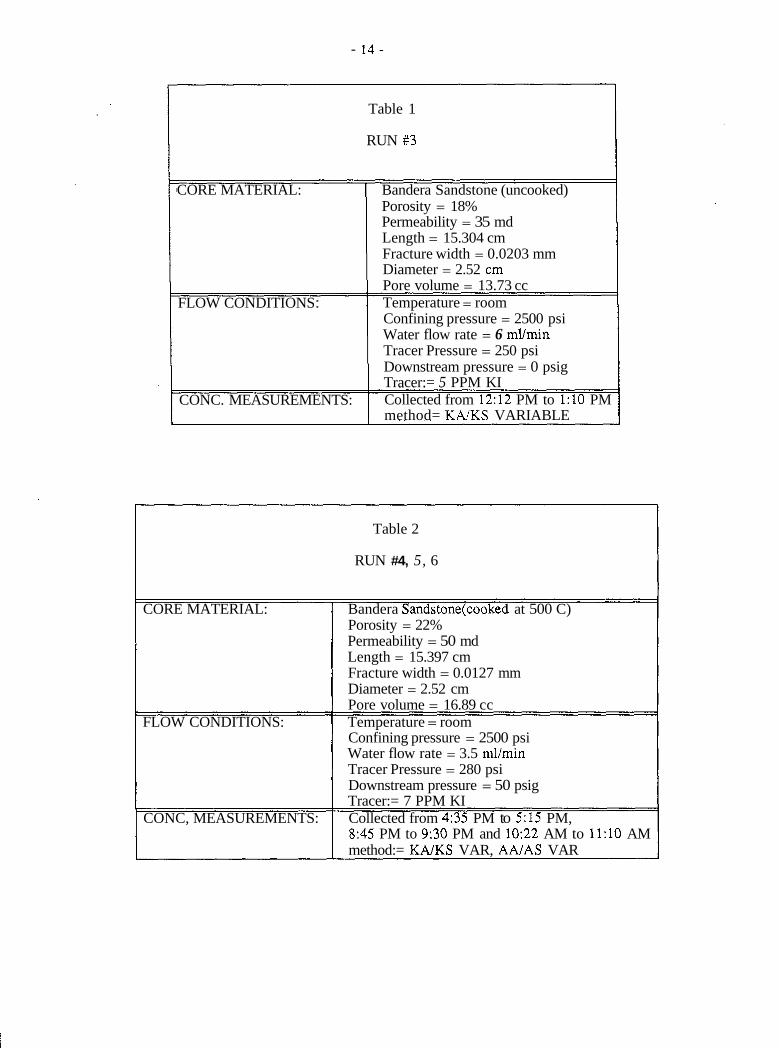
Table 1

RUN #3

CORE MATERIAL: I Bandera Sandstone (uncooked)

FLOW CONDITIONS :

CONC. MEASUREMENTS:

Porosity = 18% Permeability = 35 md Length = 15.304 cm Fracture width = 0.0203 mm Diameter = 2.52 cm Pore volume = 13.73 cc Temperature = room Confining pressure = 2500 psi Water flow rate = 6 mumin Tracer Pressure = 250 psi Downstream pressure = 0 psig Tracer:= 5 PPM KI Collected from 12:12 PM to 1:lO PM method= KNKS VARIABLE

CORE MATERIAL:

FLOW CONDITIONS:

Table 2

RUN #4, 5, 6

Bandera Sandstone(cooked at 500 C) Porosity = 22% Permeability = 50 md Length = 15.397 cm Fracture width = 0.0127 mm Diameter = 2.52 cm Pore volume = 16.89 cc Temperature = room Confining pressure = 2500 psi Water flow rate = 3.5 mllmin Tracer Pressure = 280 psi Downstream pressure = 50 psig Tracer:= 7 PPM KI Collected from 4:35 PM to 5:15 PM, 8:45 PM to 9:30 PM and 10:22 AM to 1 1 : l O AM method:= KAlKS VAR, AAIAS VAR

CONC, MEASUREMENTS:

- 15 -

Table 3

RUN #7

- CORE MATERIAL: FLOW CONDITIONS:

CONC. MEASUREMENTS:

Same as Run #4,5,6 Same as Run #4,5,6 except Temperature = 200 F Collected from 4:45 PM to 5:20 PM methnd*= K N K S VARIABLE

Table 4

RUN #8,9

:ORE MATERIAL,: FLOW CONDITIONS: Temperature = room

Same as Run #4, 5, 6

Confining pressure = 2000 psi Water flow rate = 2.8 ml/min Tracer Pressure = 290 psi Downstream pressure = 50 psig Tracer:- 20 PPM KI Collected from 4: 11 PM to 450 PM, and 6:31 PM to 6 5 5 PM method:= DIRECT, KNKS VARIABLE

ZONC. MEASUREMENTS:

Table 5

RUN #10

Tracer presure = 250 psi Downstream pressure = 50 psig

1 Tracer:= 20 PPM KI CONC. MEASUREMENTS: I Collected from 2:40 PM to 3:20 PM I method:= KNKS VARIABLE

- 16-

- E Q Q

C 0

0 L

C a, 0 C 0 0

Q) TI

U 0

v

_- t

t

_-

l-4

-0 0 H

0 10 20 30 40 Time ( m i n l

FIG. 3: Step Input of 5 PPM KI RUN #3

50 60 70

Y X

Y x x X

A

X "

X

0 5 10 15

Time (mini


20 25

- 17 -

0

10

5

0

0 5 10 15

T i m e ( m i n )

20 25


X

f i f

0 5 10 15 20 T i m e (min)


25 30

- 18 -

- € Q Q

C 0

0 L

C a, 0 C 0 0

a, 73

-0 0

v

.- e

t

--

H

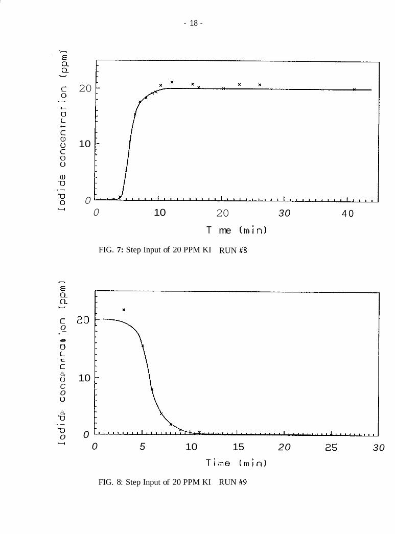
20

10

0 0

20

10

0

10 20 30 4 0

T

FIG. 7: Step Input of 20 PPM KI

me [ m i d

RUN #8

0 5 10 15 20 25 30


- 19 -

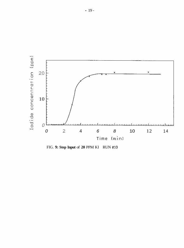
20

10

0 0 2 4 6 8 10 12 1 4

T i m e ( m i n )


- 20 -

SECTION 6: CONCLUSIONS

Experimentation that simulated tracer flow tests in fractured geothermal reservoirs

was performed and response curves were generated. By physically measuring parame-

ters of the cores used in experimentation, in this case fracture width, the validity of

Walkup’s model can be examined. The following are recommendations that could im-

prove future results:

--The Fisher ion analyzer is an accurate means of measuring sample concentra-

tions for discrete, large samples, but its application in measuring frequent and

small effluent volumes is difficult.

--By utilizing an electrode to measure conductivity and taking readings in the

flow path itself, much quicker and better defined response curves could be gen-

erated.

--A method to accurately measure and maintain the fracture width in the rock

core during the flow experiments is essential.

- 21 -

SECTION 7: REFERENCES

1.

2.

3.

4.

5.

6.

7.

8.

9.

Breitenbach, K.A., Chemical Tracer Retention in Porous Media, Stanford Geoth-

ermal Program SGP-TR-53, Stanford University, May 1982.

Bouett, L., Draft of Masters Report, December 1985.

Fisher Scientific Company, Fisher Accumet Selective Ion Analyzer Model 750 In-

struction Manual, Pittsburgh, Pennsylvania, 1984.

Fossum, M.P., Tracer Analysis in a Fractured Geothermal Reservoir: Field

Results from Wairakei, New Zealand, Stanford Geothermal Program SGP-TR-56,

Stanford University, June 1982.

Fossum, M.P., Home R.N., "Interpretation of Tracer Return Profiles at Wairakei

Geothermal Field Using Fracture Analysis," Geothermal Resources Council Tran-

sactions Vol. 6, pp. 261-264, 1982.

Gilardi, J.R., Experimental Determination of the Effective Dispersivity in a Frac-

ture, Stanford Geothermal Program SGP-TR-78, Stanford University, June 1984.

Horne, R.N., Rodriguez, F., "Dispersion in Tracer Flow in Fractured Geothermal

Systems," Geophysical Research Letters, Vol. 10, No. 4, pp. 289-292, April 1983.

Jackson, P.B., Method for the Collection and Analysis of Sample Fluids During a

Tracer Test, Stanford Geothermal Program, SGP-TR-XX, Stanford University,

June 1982.

Jensen, C.L., Matrix Diffusion and its Effects on the Modeling of Tracer Returns

from the Fractured Geothermal Reservoir at Wairakei, New Zealand, Stanford

Geothermal Program SGP-TR-71, Stanford University, December 1983.

- 22 -

10. Jensen, C.L., Home R.N., "Matrix Diffusion and its Effect on the Modeling of

Tracer Returns from the Fractured Geothermal Reservoir at Wairakei, New Zea-

land," Ninth Workshop on Geothermal Reservoir Engineering, SGP-TR-74, Stan-

ford University, December 1983.

11. Neretnieks, I., Eriksen, T., Tahtinen, P., "Tracer Movement in a Single Fissure in

Granite Rock: Some Experimental Results and Their Interpretation," Water

Resources Research, Vol. 18, No. 4, pp. 849-858, 1982.

12. Sageev, A., Design and Construction of an Absolute Permeameter to Measure the

Effect of Elevated Temperature on the Absolute Permeability to Distilled Water

of Unconsolidated Sand Cores, Stanford Geothermal Program SGP-TR-43, Stan-

ford University, December 1980.

13. Walkup, G.W., Jr., Characterization of Retention Processes and their Effects on

the Analysis of Tracer Tests in Fractured Reservoirs, Stanford Geothermal Pro-

gram SGP-TR-77, Stanford University, June 1984.

14. Walkup, G.W., Jr., Home, R.N., Characterization of Retention Processes and their

Effects on the Analysis of Tracer Tests in Fractured Reservoirs, Society of

Petroleum Engineers Technical Paper #13610, 1985.

- 23 -

SECTION 8: APPENDIX

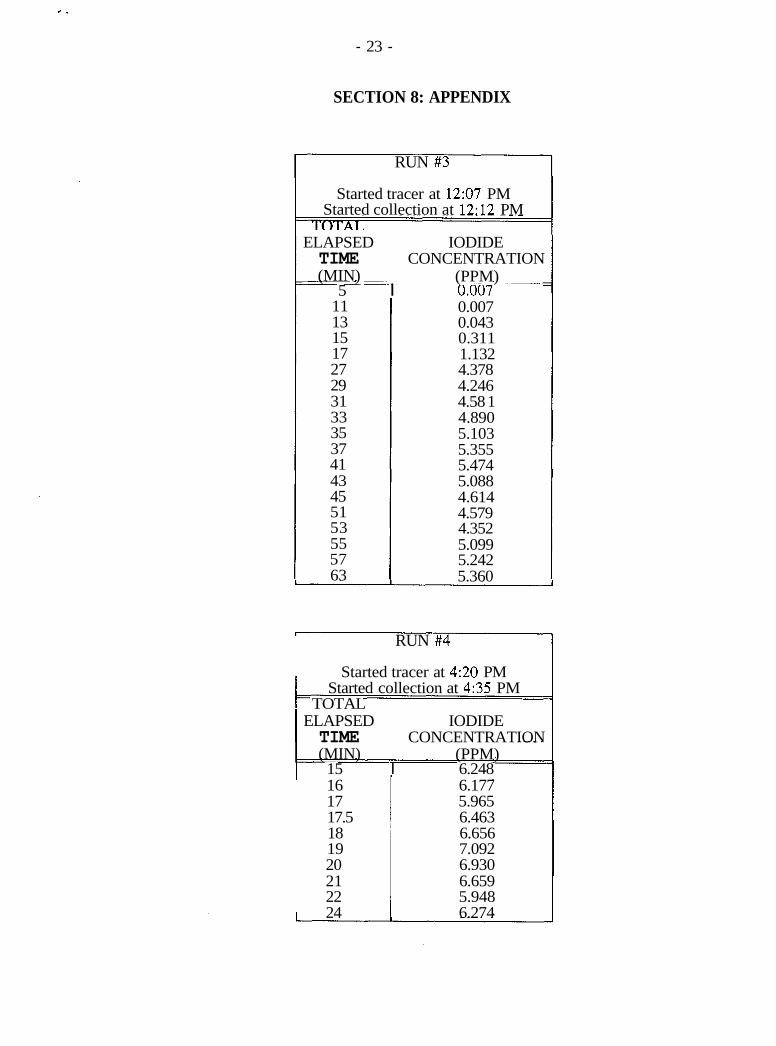
RUN #3

Started tracer at 12:07 PM Started collection at 12:12 PM

ELAPSED IODIDE TIME CONCENTRATION (MIN) (PPM)

5 I 0.007 11 13 15 17 27 29 31 33 35 37 41 43 45 51 53 55 57 63

0.007 0.043 0.311 1.132 4.378 4.246 4.58 1 4.890 5.103 5.355 5.474 5.088 4.614 4.579 4.352 5.099 5.242 5.360

RUN #4


TOTAL ELAPSED IODIDE I TIME CONCENTRATION

(MIN) (PPM) 15 I 6.248 16 6.177 17 5.965 17.5 6.463 18 6.656 19 7.092 20 6.930 21 6.659 22 5.948 24 6.274

- 24 -

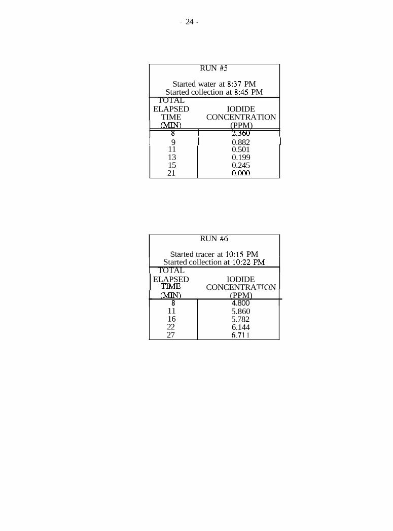
RUN #5

Started water at 8:37 PM Started collection at 8:45 PM

TOTAL ELAPSED IODIDE

TIME CONCENTRATION (MIN) (PPM)

8 I 2.360 I 9 I 0.882 I

11 13 15 21

0.501 0.199 0.245 0.000

RUN #6

Started tracer at 10:15 PM Started collection at 1022-PM

TOTAL ELAPSED IODIDE I CONCENTRATION ~ ~ _ _

- (MIN) (PPM) 8 1 4.800

11 16 22 27

5.860 5.782 6.144 6.71 1

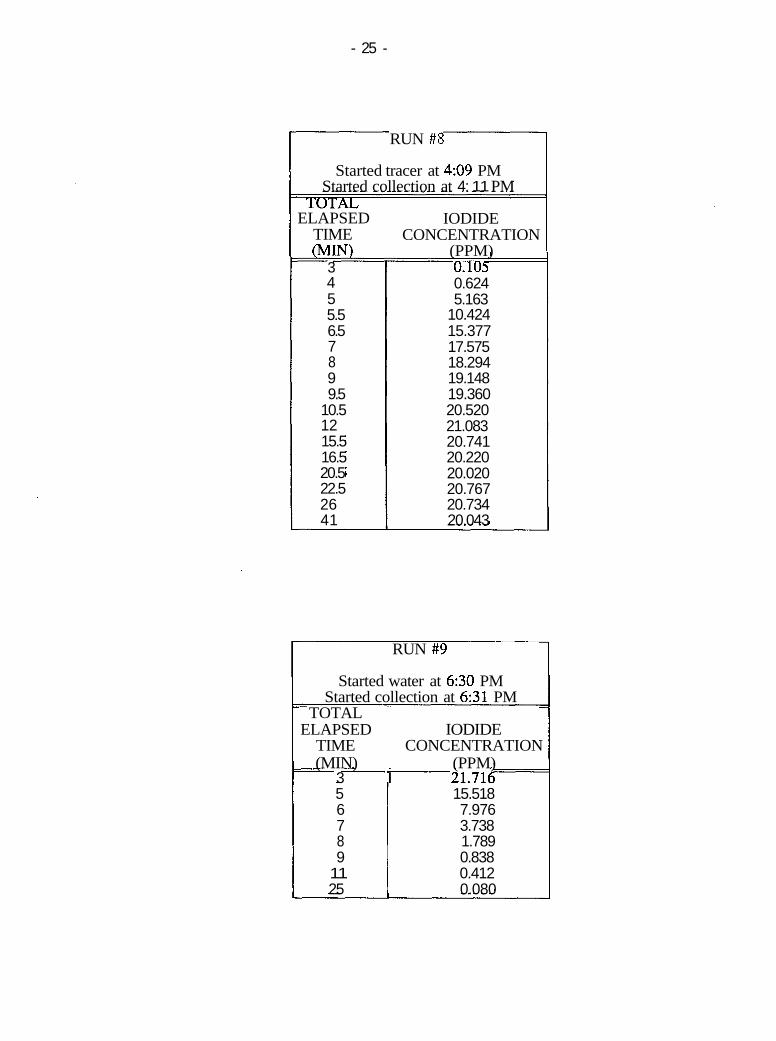
- 25 -

RUN #8

Started tracer at 4:09 PM Started collection at 4: 11 PM

ELAPSED TIME (MIN)

3 4 5 5.5 6.5 7 8 9 9.5

10.5 12 15.5 16.5 20.5 22.5 26 41

IODIDE CONCENTRATION

(PPM) 0.1u3 0.624 5.163

10.424 15.377 17.575 18.294 19.148 19.360 20.520 21.083 20.741 20.220 20.020 20.767 20.734 20.043

RUN #9

Started water at 6:30 PM Started collection at 6:31 PM

TOTAL ELAPSED IODIDE

TIME CONCENTRATION (MIN) (PPM)

3 I 21.’/16 5 15.518 6 7.976 7 3.738 8 1.789 9 0.838

11 0.412 25 0.080

- 26 -

RUN #10


LOTAL ELAPSED TIME (MIN) 1

2 3 4 5 6.5 7 8

12

IODIDE CONCENTRATION

(PPM) 0.000 0.012 7.827

16.915 18.726 19.572 19.593 20.290 20.500

Documents

The Generation of Response Curves from Laboratory Tracer