The global SMOS Level 3 daily soil moisture and …archimer.ifremer.fr/doc/00388/49941/50526.pdf · in France and Centro para el Desarrollo Tecnológico ... Marquardt optimisation

Earth Syst. Sci. Data, 9, 293–315, 2017https://doi.org/10.5194/essd-9-293-2017© Author(s) 2017. This work is distributed underthe Creative Commons Attribution 3.0 License.

The global SMOS Level 3 daily soil moisture andbrightness temperature maps

Ahmad Al Bitar1,2, Arnaud Mialon1,2, Yann H. Kerr1,3, François Cabot1,3, Philippe Richaume1,Elsa Jacquette3, Arnaud Quesney4, Ali Mahmoodi1, Stéphane Tarot5, Marie Parrens1, Amen Al-Yaari6,

Thierry Pellarin7, Nemesio Rodriguez-Fernandez1, and Jean-Pierre Wigneron6

1Centre d’Etudes Spatiales de la Biosphère, Université de Toulouse, CNES/CNRS/IRD/UPS, Toulouse, France2Centre National de Recherche Scientifique, Paris, France

3Centre National d’Etudes Spatiales, Paris, France4CapGemini Sud, 109 Avenue du Général Eisenhower, 31000 Toulouse, France

5IFremer, BP 70, 29280 Plouzane, France6INRA, UMR1391 ISPA, Villenave d’Ornon, France

7IGE, University Grenoble Alpes, CNRS/G-INP/IRD/UGA, Grenoble, France

Correspondence to: Ahmad Al Bitar ([email protected])

Received: 4 January 2017 – Discussion started: 10 February 2017Revised: 18 April 2017 – Accepted: 19 April 2017 – Published: 6 June 2017

Abstract. The objective of this paper is to present the multi-orbit (MO) surface soil moisture (SM) and angle-binned brightness temperature (TB) products for the SMOS (Soil Moisture and Ocean Salinity) mission basedon a new multi-orbit algorithm. The Level 3 algorithm at CATDS (Centre Aval de Traitement des DonnéesSMOS) makes use of MO retrieval to enhance the robustness and quality of SM retrievals. The motivation ofthe approach is to make use of the longer temporal autocorrelation length of the vegetation optical depth (VOD)compared to the corresponding SM autocorrelation in order to enhance the retrievals when an acquisition occursat the border of the swath. The retrieval algorithm is implemented in a unique operational processor deliveringmultiple parameters (e.g. SM and VOD) using multi-angular dual-polarisation TB from MO. A subsidiary angle-binned TB product is provided. In this study the Level 3 TB V310 product is showcased and compared toSMAP (Soil Moisture Active Passive) TB. The Level 3 SM V300 product is compared to the single-orbit (SO)retrievals from the Level 2 SM processor from ESA with aligned configuration. The advantages and drawbacksof the Level 3 SM product (L3SM) are discussed. The comparison is done on a global scale between the twodatasets and on the local scale with respect to in situ data from AMMA-CATCH and USDA ARS Watershednetworks. The results obtained from the global analysis show that the MO implementation enhances the numberof retrievals: up to 9 % over certain areas. The comparison with the in situ data shows that the increase inthe number of retrievals does not come with a decrease in quality, but rather at the expense of an increasedtime lag in product availability from 6 h to 3.5 days, which can be a limiting factor for applications like floodforecast but reasonable for drought monitoring and climate change studies. The SMOS L3 soil moisture and L3brightness temperature products are delivered using an open licence and free of charge using a web application(https://www.catds.fr/sipad/). The RE04 products, versions 300 and 310, used in this paper are also available atftp://ext-catds-cpdc:[email protected]/Land_products/GRIDDED/L3SM/RE04/.

Published by Copernicus Publications.

https://www.catds.fr/sipad/

ftp://ext-catds-cpdc:[email protected]/Land_products/GRIDDED/L3SM/RE04/

294 A. Al Bitar et al.: The global SMOS Level 3 daily soil moisture and TB maps

1 Introduction

Surface soil moisture (SM) is a control physical parameterfor many hydrological processes like infiltration, runoff, pre-cipitation and evaporation (Koster et al., 2004). Estimatesof SM are needed for many applications concerned withmonitoring droughts (Keyantash and Dracup, 2002), floods(Brocca et al., 2010; Lievens et al., 2015), weather fore-cast (Drusch, 2007; de Rosnay et al., 2013), climate (Jung etal., 2010) and agriculture (Guérif and Duke, 2000). It is iden-tified among the 50 Essential Climate Variables (ECVs) forthe Global Climate Observing System (GCOS). It has alsobeen selected for the creation of decadal (10 years) time se-ries from remote sensing in the ESA Climate Change Initia-tive (CCI) project (Hollmann et al., 2013).

SM can be obtained from several Earth observation (EO)techniques ranging from visible to microwave wavelengthsusing active (Ulaby et al., 1996) and passive (Kerr andNjoku, 1990) instruments. Retrieval of SM from passive mi-crowave sensors is a challenging task because features likesurface heterogeneity (water surfaces and land use), vegeta-tion cover (vegetation density and distribution), climatic con-ditions (freezing and snow), acquisition configurations (an-gle, frequency and polarisation) and topography (multiplescattering) need to be carefully considered while upscaling tothe sensor coarse resolution. Several approaches like regres-sion models (Njoku et al., 2003; Wigneron et al., 2004; Salehet al., 2006), statistical and contextual methods (Verhoestet al., 1998), neural networks (Liu et al., 2002; Rodríguez-Fernández et al., 2015), and radiative-transfer-based ap-proaches (Kerr and Njoku, 1990; Wigneron et al., 2007;Owe et al., 2008; O’Neill et al., 2015) have been developedto retrieve SM based on the sensor frequency, acquisitionmodes and richness of information (multi-angular, full po-larisation and active). The Soil Moisture and Ocean Salinity(SMOS) mission of ESA (Kerr et al., 2001, 2010) with con-tributions from Centre National d’Etudes Spatiales (CNES)in France and Centro para el Desarrollo Tecnológico Indus-trial (CDTI) in Spain is the first Earth observation missiondedicated to SM mapping. The SMOS Level 2 (L2) SM re-trieval algorithm (Kerr et al., 2012) minimizes the squareddifferences between L-MEB (Wigneron et al., 2007) for-ward simulations of multi-angular dual-polarisation TB andcorresponding SMOS measurements using the Levenberg–Marquardt optimisation algorithm to retrieve physical pa-rameters, mainly SM and VOD.

The L-MEB radiative transfer model is based on the opti-cal depth single-scattering albedo (τ–ω) emission model (Moet al., 1982) combined with specific parameterisations to takeinto account the impact of vegetation and soil roughness onpolarisation mixing and angular signature. The Soil Mois-ture Active Passive (SMAP) mission, launched by NASAin January 2015, delivers TB observations at a fixed (40◦)incidence angle (Entekhabi et al., 2010). The SMAP soilmoisture processor currently relies on a single-channel al-

gorithm (SCA) (O’Neill et al., 2015) for its main product.This algorithm uses a forced VOD in a single-orbit configura-tion. Miernecki et al. (2014) and Wigneron et al. (2017) pre-sented a review and a comparison of the different retrieval ap-proaches for L-band microwave from EO missions (SMOS,SMAP and AQUARIUS).

Passive microwave sensors have a high revisit frequency:1 day for Advanced Microwave Scanning Radiometer - EarthObserving System (AMSR-E) (Njoku and Entekhabi, 1996)and 2–3 days for SMOS and SMAP. In this study the multi-orbit (MO), multi-angular and dual-channel horizontal andvertical (H/V) operational retrieval algorithm implemented atthe CATDS (Centre Aval de Traitement des Données SMOS)by CNES is presented. Retrieval using temporal series is be-coming increasingly common in operational EO retrieval al-gorithms for optical and to some extent microwave technolo-gies. Some examples in the optical domain are the correctionof aerosol impact for visible images (Hagolle et al., 2008,2015), cloud detection (Hagolle et al., 2010) and the useof MO for land cover classification (Inglada and Mercier,2007). The previous methodologies are being implementedfor high-end level 2-A and level 3 products for the Coper-nicus Sentinel-2 mission. The use of MO in the radar com-munity is a standard approach. The SM retrievals from ERS(European Remote Sensing), Advanced Scatterometer (AS-CAT), RADARSAT-2 and Sentinel-1 are based on a changedetection algorithm (Wagner et al., 1999, 2013; Naeimi etal., 2009). Similarly, Mattia et al. (2006) introduced a pri-ori surface parameters and multi-temporal synthetic apertureradar (SAR) data to reduce the impact of vegetation and soilroughness in SM retrieval from SAR. Recently, a generalisa-tion of change detection to multiple regression using cumula-tive distribution function (CDF) transformations was appliedto RADARSAT-2 time series data and validated over the Be-rambadi watershed, South India (Tomer et al., 2015). In mi-crowave radiometry, Konings et al. (2016) presented a timeseries retrieval of vegetation optical depth based on AQUAR-IUS L-band acquisitions.

Here a detailed presentation of the products and retrievalalgorithm of an inter-comparison between the SMOS SO(single-orbit) and the SMOS MO (multi-orbit) operationalproducts is given. More specifically, the objective of this pa-per is to present the daily L3 SM and TB V310 productsand associated algorithms and to compare the SMOS MOlevel 3 retrievals to the level 2 single-orbit operational re-trievals obtained using V600 L1 ESA-SMOS products. Sincethe SMOS mission launch in November 2009, this is the firstreprocessing to have an aligned version of the processorsfrom Level 1 up to Level 3, enabling a direct comparisonof the products. In the next sections the MO retrieval SM al-gorithm and the L3 TB are presented. The datasets used forthe assessment, the results of the comparison and conclusionsare presented.

Earth Syst. Sci. Data, 9, 293–315, 2017 www.earth-syst-sci-data.net/9/293/2017/

A. Al Bitar et al.: The global SMOS Level 3 daily soil moisture and TB maps 295

2 The CATDS Level 3 soil moisture processor

2.1 Algorithm overview

The Level 3 SM (L3SM) processor consists of a set of sev-eral algorithms. The forward model in L3SM uses the samephysically based forward models as the ESA SMOS Level 2SM processor, but in a MO retrieval context. A short sum-mary of the main features of this processor is provided hereand a detailed description can be found in Kerr et al. (2012).The SMOS L2 retrieval can be divided into two main com-ponents:

1. The first component is a physical model that computesTB at the antenna reference frame forced by ancillarydata (land classification and soil properties) and phys-ical parameters (skin or near-surface temperature andsoil temperature). The selected physical model for theSMOS mission is L-MEB from Wigneron et al. (2007).The main features of the L-MEB physical model im-plementation in the SMOS operational processor are asfollows:

– Effective scattering albedo is considered.

– SM and VOD are jointly retrieved over nominal(bare soil and low vegetation) surfaces using angu-lar signature and polarisation information.

– Dual polarisation is used. Full polarisation data areonly used to take into account the Faraday rotationand geometric rotation to transform modelled TBfrom the top of atmosphere (TOA) to the antennareference frame.

– The mean antenna pattern (Kerr et al., 2012) isused in the iterative retrieval algorithm. The meanweighting function expresses the average contribu-tions for all angular acquisitions. The −3 dB foot-prints are about 20 km in radius. This correspondsto the nominal resolution of the synthetic aper-ture. This also corresponds to 86 % of the signalif a homogeneous surface is considered (Al Bitar etal., 2012).

– Surface heterogeneity is considered through ag-gregated TB contributions from 4× 4km2 surfaceunits. The contributions are then convoluted withthe mean antenna pattern. A total area of 125×125km2 is considered at each retrieval node tocompute the total emissions.

– Dynamic changes in surface state (freezing, rain-fall, etc.) are considered through the use of ancillaryweather data from ECMWF reanalysis products.Since the mission launch, many improvements havebeen implemented in the operational processingmodel. Some examples include, for instance, theimproved parametrization of the forest albedo in

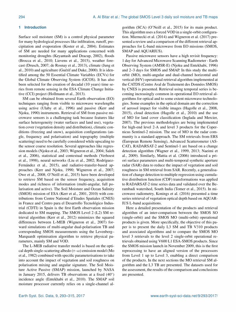
Figure 1. Number of TB records across the swath for a period of8 days – from 18 to 25 May 2010 – over the area of La Plata, Ar-gentina.

Rahmoune et al. (2014) or the choice of dielectricmixing models in Mialon et al. (2015).

2. The second component of the retrieval algorithm is aniterative optimisation scheme that minimises a Bayesiancost function constructed from the observed and themodelled TBs in order to retrieve the physical param-eter values. Preprocessing and post-processing steps areimplemented to filter the input and output data for un-desired effects like the decrease in quality due to spatialsampling or radio frequency interferences (RFIs) (Olivaet al., 2012; Richaume et al., 2014).

The physical approach at Level 3 MO is the same as thatof Level 2 SO. In fact the core processing uses the sameimplementation of the L-MEB radiative transfer model.The main difference in Level 3 is the use of several or-bits, rather than one, to retrieve SM and VOD. This hasan impact first on the post-processing steps for select-ing the orbits and second on the optimisation schemeto retrieve the parameters. Since the Level 2 retrieval isa multi-parameter retrieval, the Level 3 is thus a multi-orbit multi-parameter retrieval. The reasons that moti-vated the use of the MO approach are the following:

– The angular sampling and radiometric accuracy atthe border of the swath are reduced. Figure 1 showsthe cumulative number of records for several de-scending orbits. The asterisk in each panel repre-sents the same location in the La Plata region inSouth America. The orange regions inside the or-bits observed on 18, 20 and 23 May 2010 depict themild decrease in the number of TB measurements(15–35) during the instrument calibration phases.However, most important is the low number of TBmeasurements (35) observed on 21 May when the

www.earth-syst-sci-data.net/9/293/2017/ Earth Syst. Sci. Data, 9, 293–315, 2017


point of interest is at the border of the swath. Alow number of TB measurements spanning a nar-row range of incidence angles generates failures inthe iterative retrieval of SM and VOD. The use ofMO can help improve the number of successful re-trievals at the border of the swath.

– The VOD is expected to vary slowly in time andthus to be highly correlated between two consecu-tive ascending or descending orbits or over a shortperiod of time (a few days). In fact, at L band theVOD is mainly correlated to vegetation water con-tent (Jackson and Schmugge, 1991), which is ex-pected to vary slowly in time compared with tem-poral variability in SM.

Other general motivations for Level 3 products are toprovide a global gridded product, in contrast to swath-based products and to provide fixed-angle-binned TBproducts. The 25 km Equal-Area Scalable Earth Gridversion 2.0 (EASE-Grid 2.0) (Brodzik and Knowles,2002), which was selected for the Level 3 MO prod-uct also has a spatial sampling closer to the sensor’snominal resolution. The main input TB for the process-ing is generated from the snapshot-based L1B products,which are TBs in the Fourier domain. This consists of aninverse fast Fourier transform (IFFT) to make the tran-sition from the Fourier domain to the spatial domain us-ing the L3 EASE-Grid 2.0. In a subsequent step, TBmeasurements corresponding to the same grid point areselected from the different snapshots (for a given gridpoint, the incidence angle of the observation is differentfor each snapshot) to construct a grid-point-based prod-uct similar to the ESA L1C TB product but in EASE-Grid 2.0. The alternative is to interpolate the ESA L1CTB dataset from the 15 km Icosahedral Snyder EqualArea (ISEA) grid to the 25 km EASE-Grid 2.0 grid. Thisoption was excluded because it could have generated in-terpolation artefacts on the TB products that would havepropagated through the processing chain.

2.2 Orbit selection

The selection of orbits is needed to select TBs at high lati-tudes where a sub-daily revisit is available and to generatethe time series dataset on the EASE-Grid 2.0 as input to theMO retrieval. The following criteria are applied for the se-lection of revisits:

– Ascending and descending orbits are processed sepa-rately since the impact of RFI (Oliva et al., 2012) andsun corrections (Khazâal et al., 2016) between ascend-ing and descending orbits are very different.

– TB products are filtered at high latitudes where morethan one revisit per day occurs (latitudes above 60◦ N

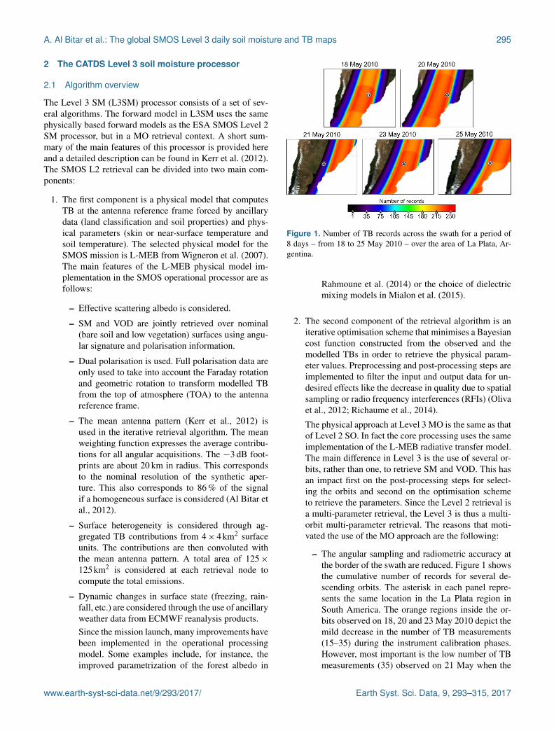
Figure 2. Selection of revisit orbits for the multi-orbit retrieval atSMOS CATDS.

and 60◦ S). A maximum of one revisit per day is con-sidered. The selection criterion is the minimum distancefrom the centre of the swath because the radiometric ac-curacy and resolution is best at the centre. This criterionis applied for each grid node individually.

At this level the acquisitions for a given day for ascend-ing and descending orbits are separately stored in a three-dimensional matrix accounting for snapshots, longitude andlatitude. A snapshot is an image associated to the acquisitionof SMOS during a given integration time (epoch). Snapshotshave different epochs and polarisation following a prepro-grammed acquisition sequence. From this product a fixed-angle-binned TB product is generated as presented in Sect. 3.The product is also used in the next processing steps of L3SMMO.

– For each retrieval and over each node a 7-day periodis considered in which three revisits are selected fromthe complete list of revisits (Fig. 2). The first coincideswith the central date (date of main product). The twoothers correspond to selected dates either before (previ-ous 3.5 days) or after (3.5 days posterior) the considereddate. Like in the previous processing step, the selectionis done based on minimum distance from the swath cen-tre for each node.

2.3 Cost function and retrieval

Observed TBs at the antenna reference frame from the prece-dent, actual and succeeding dates are assembled for eachnode. The forward algorithm is run to generate the modelledTB for each of the TB dataset records. The ancillary data andparameters are independently considered for each record. ABayesian cost function that includes the aforementioned MOobserved TB and modelled TB is then constructed. This isachieved by incorporating in the retrieval approach a tempo-ral autocorrelation function for the VOD. The cost function



is as follows:

Cost= (TBM−TBF)t·COV−1

TB · (TBM−TBF)

+

∑p

(P −P0)t·COV−1

p · (P −P0) , (1)

where COVTB = σ2TB is the error covariance matrix of TB

data when assuming no auto-temporal correlation, TBM isthe measured TB from SMOS, TBF is the forward modelledTB using L-MEB, P is the vector of retrieved parameters(SM and VOD) at the three times of acquisition, COVP isthe error covariance matrix for parameter P and P0 is the apriori value of parameter P .

It is important to note that three SM values are retrievedsimultaneously at each node: SMP for the preceding date,SMA for the actual date and SMF for the succeeding date.The same applies to VOD. In the case of SM, the a priorivalues are retrieved from ECMWF reanalysis data.

Where P = [SMP,SMA,SMF], the error covariance ma-trix considering no cross- or autocorrelation is given by

COVSM = σ2SM0 · I, (2)

where σ 2SM0 is the standard-deviation error associated with

SM. It is set to a high value: 0.7 m3 m−3. I is the (3×3) iden-tity matrix.

When P is equal to VOD, the error covariance matrix,considering temporal autocorrelation and no cross correla-tion between the different parameters, is given by

COVVOD = σ2VOD0

1 . . . . . .

ρ (tP, tA) 1 . . .

ρ (tP, tF) ρ (tA, tF) 1

, (3)

where σ 2VOD0

is the standard-deviation error associated withVOD, and ρ is the correlation function modelled assuming aGaussian autocorrelation distribution:

ρVOD (t1, t2)= ρmax (t1, t2) · exp

(−

(t1− t2)2

T 2c

), (4)

where t1 and t2 are the times (expressed in days) correspond-ing to the VOD retrieval dates (P, A or F), ρmax(t1, t2) is themaximum amplitude of the correlation function between t1and t2 and Tc is the characteristic correlation time for VOD(Tc = 30 days for forests and Tc = 10 days for low vegeta-tion).

Figure 3 shows the shape of the correlation function forthe two correlation lengths used in the processing. The greencurve corresponds to the forested surfaces and the blue oneto the nominal surfaces (bare soil and low vegetation).

The parameter values namely (SMP, SMA, SMF, VODP,VODA and VODF) are retrieved by minimising the cost func-tion in an iterative procedure using the Levenberg–Marquardtoptimisation algorithm. Thus, at the end of each daily re-trieval, three SM values are available. The retrieval associ-ated with the best goodness of fit (X2) value is then selected

Figure 3. Autocorrelation functions for vegetation optical depth(VOD) for different correlation lengths (green shows forested sur-faces and blue shows nominal surfaces).

and delivered in the 1-day product. This product is only avail-able when the filtering is finished, and thus with 7 days of lagtime. Using the daily maps, time synthesis products (3 days,10 days and monthly) are then provided. A detailed descrip-tion of the algorithm is presented in the CATDS L3 Algo-rithm Theoretical Basis Document (Kerr et al., 2013).

3 The CATDS Level 3 angle-binned TB processor

The objective of this algorithm is to generate a product con-taining fixed-angle full-polarisation brightness temperaturesat top of atmosphere (TOA) but with the polarisations ex-pressed in the ground reference frame (horizontal and ver-tical components) over the EASE-Grid 2.0. The main inputfor this algorithm is the snapshot dataset mentioned in theprevious section. The algorithm consists of four steps: (a) fil-tering, (b) interpolation, (c) reference frame transformationand (d) angle binning. However, note that before being pro-jected to a ground reference frame, the data are processed inthe instrument reference frame. Thus, TBs are labelled TBYand TBX to express that the polarisations are at satellite level,while once processed they will be provided in the ground ref-erence frame and will be labelled TBH and TBV.

3.1 TB filtering

The filtering eliminates brightness temperatures that are im-pacted by anthropogenic effects (such as RFIs), or spuriouseffects (such as sun impact). The filtering criteria, shown inTable 1, are similar to those for L3 MO SM and L2 SO re-trievals. A detailed description of the filtering criterion is pro-vided in the SMOS L2 ATBD (Algorithm Theoretical BasisDocument). The reader can refer to Khazaal et al. (2016) fora more detailed evaluation of the impact of sun correctionsand Richaume et al., 2014 and Soldo et al., 2014 for the im-



Table 1. List of applied filtering criterion used on brightness tem-perature products prior to interpolation.

Filtering criteria Applied test

Thresholds50 K<TBX and TBY < 340 K−50 K<TBxy <+50 K

Amplitude 50 K<√

TB2x +TB2

y < 500 K

Standard deviation TB – 2 ·ATB<TB<TB+ 2·ATB

First Stokes ST1−ST1< 5+ 4·ATB

SMEF< (55× 55) km2

Spatial resolutiona Lma/Lmi< 1.5BORDER FOV (flag is off)

RFI

L1A STRONG RFI (flag is off)L1B STRONG RFI (flag is off)POINT SOURCE RFI (flag is off)TAILS RFI (flag is off)

Sun correctionb SUN_POINT (flag is off)SUN_TAILS (flag is off)

ATB is the radiometric accuracy of SMOS TB, ST1 is the first Stokesparameter, ST1 is the average of ST1 over each dwell line (angularsignature), ST4 is the fourth Stokes parameter, SMEF is the area of thehalf-maximum contour of the mean synthetic antenna pattern, Lma is thelength of the major axis of the synthetic antenna pattern and Lmi is the lengthof the minor axis of the synthetic antenna pattern.a Spatial resolution eliminates records that are impacted by aliasing (onlyalias-free field of view is considered).b If active the flag means that the pixel is located in a zone where a sun aliaswas reconstructed (after sun removal, measurement may be degraded). Thesun tail is considered when the pixel is located in the hexagonal aliasdirections centred on a sun alias.

pact of RFIs. All filtering criteria should be met, otherwisethe acquisition is discarded. In case a cross polarisation isdiscarded, the associated X and Y acquisitions are also re-moved.

3.2 TB interpolation

The acquisition sequence of SMOS is shown in Table 2. Ateach epoch an acquisition can be co-polarised (X, Y ) or com-bined cross (XY , YX) and co-polarised. The table shows thatthere is no complete dataset for any epoch. A weighted lin-ear interpolation is used to compute the missing acquisitionsbased on adjacent ones.

The weighting function accounts for the two following el-ements:

– The TB acquisitions have different accuracy levels sincethe integration time is longer when only co-polarisationis acquired (pure acquisition) when compared to thecase where combined cross and co-polarisation are ac-quired.

– The time span between two acquisitions in the samemode is not constant. Acquisitions closer in time areconsidered more reliable than farther ones, taking into

consideration that the synthetic antenna weighting func-tion rotates and that the incidence angle changes.

The time interpolation function of TB at time i (TBi) is asfollows:

TBi =Wi−1 ·TBi−1+Wi+1 ·TBi+1

Wi−1+Wi+1

Wi−1 =1

σi−1 · nb_epoi−1

Wi+1 =1

σi+1 · nb_epi+1

, (5)

where nb_epoi is the number of epochs between acquisitionsat time i, σ is the corresponding radiometric accuracy andWi is the weighting coefficient at time i. The standard devia-tion of the interpolated field is computed based on the squareroot of the weighted variances of the adjacent acquisition.We assume that the acquisitions are not correlated; therefore,no cross correlation term is considered in the equation. Thefollowing formulation is used:σi =

√(Qi−1 · σi−1)2

+ (Qi+1 · σi+1)2

Q2i−1+Q

2i+1

Qi =1

nb_epoi

. (6)

The same approach as Eq. (5), while applying a constantweight, is used to compute the interpolated values of aux-iliary information such as major and minor semi-axis length,incidence angle, Faraday angle and geometric angle.

3.3 Transformation from antenna to ground referenceframe

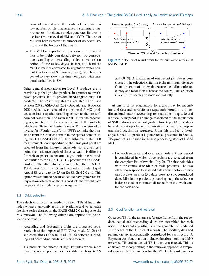
In this step, the TBs are transformed from the antenna ref-erence frame (X, Y ) to the ground reference frame (H, V).This is done without accounting for atmospheric and galac-tic contributions. They are considered as TOA TBs. The TBcomponents at antenna reference frame exhibit polarisationmixing due to the geometry of the acquisition (Fig. 4). Fara-day rotation will also slightly alter the polarisations.

The inverse of the rotation matrix is used to transform theTB data from antenna to ground reference frame:

TBHTBVTB3TB4

= IRM

TBXTBY

2 · real (TBXY )−2 · imag(TBXY )

. (7)

TB3 and TB4 are the Stokes 3 and Stokes 4 components. Theinverse of rotation matrix (IRM) is given by

IRM=

cos2a sin2a cosa · sina 0sin2a cos2a −cosa · sina 0−sin2a sin2a cos2a 0

0 0 0 1

, (8)



Table 2. Acquisition sequences of SMOS in full polarisation mode (capital letters are used for pure acquisition).

Snapshot number 1 2 3 4 5 6 7 8 9 10 11 12

TB (real/imaginary) X/XY Y /YX X/XY Y /YXTB (co-polarisation) X X Y y X x Y X Y Y

Figure 4. Transformation from antenna (S) to ground referenceframe (G). ωf is the Faraday rotation angle and2g is the geometricrotation angle (adapted from SMOS L2 ATBD).

where

a =2g+ωf , (9)

with2g being the geometric angle and ωf being the Faradayrotation angle as shown in Fig. 4.

The accuracies of the TB data are then computed by prop-agating the accuracies using the matrix below:

σTBH =(IRM2

1,1 · σTB2X + IRM2

1,2 · σdTB2Y

+4 ·(IRM2

1,3+ IRM21,4)· σTB2

XY

)0.5σTBV =

(IRM2

2,1 · σTB2X + IRM2

2,2 · σdTB2Y

+4 ·(IRM2

2,3+ IRM22,4)· σTB2

XY

)0.5σTB3 =

(IRM2

3,1 · σTB2X + IRM2

3,2 · σdTB2Y

+4 ·(IRM2

3,3+ IRM23,4)· σTB2

XY

)0.5σTB4 =

(IRM2

4,1 · σTB2X + IRM2

4,2 · σdTB2Y

+4 ·(IRM2

4,3+ IRM24,4)· σTB2

XY

)0.5, (10)

where IRMi,j are the ith column and j th row components ofthe IRM matrix.

3.4 Angle binning

This step consists in averaging the TOA TBs at fixed-angleintervals using an arithmetic mean. The selected incidenceangle bins, shown in Table 3, are designed to also cover theSMAP acquisition angle (40◦).

All TB values outside the interval defined by mean(TB)± 2 SD (TB) are considered as outliers and removedfrom the binning. The SD (TB) corresponds to the standarddeviation of TB values inside each angle bin, not to be con-fused with the radiometric accuracy. The filtered outlier val-ues are mainly associated with low RFI effects. If one com-ponent of TB (TBH, TBV and TBHV) is filtered out, all theother components are disregarded.

4 Datasets

4.1 Remote sensing datasets

4.1.1 SMOS CATDS Level 3 soil moisture products

The CATDS Level 3 user data products (CLF3UA/D) are MOsoil moisture retrieval products. They contain 1-day globalmaps of geophysical parameters (SM, VOD, imaginary andreal part of the dielectric constant, etc.) retrieved as describedabove, processing parameters (percentage of forest cover,choice of physical model, etc.) and quality indicators (prob-ability of RFI, goodness of fit between modelled TB fromL-MEB and observed TB X2, etc.) over continental surfacesfor ascending and descending orbits separately. They are inthe netCDF format over the EASE-Grid 2.0 25 km and gener-ated at the Institut Français de Recherche pour l’Exploitationde la Mer (IFREMER) for CNES and distributed via theCATDS web portal (http://www.catds.fr) and ftp server. Theoperational production of L3SM started in 2010 and it iscurrently ongoing. The time span used in this study covers2010–2015 for the global maps and 2010–2016 for the timeseries analysis. The user has access to the latest versions ofthe products from reprocessing and operational processing.The current study uses the latest data corresponding to repro-cessing RE04, which uses CATDS V300 corresponding toESA V620 Levels 1 and 2. It is the first simultaneous Level 2and Level 3 reprocessing campaign since the start of the mis-sion. Previous versions of the L3SM products where com-pared to soil moisture products from AMSR-E (Al-Yaari etal., 2014a) and ASCAT (Al-Yaari et al., 2014b) missions, butthis is the first comparison enabling an aligned configurationof the L2SM SO and L3SM MO. It has homogenised inputs(L1B/C) and physical parametrization. It uses the Mironovmodel to relate soil liquid water content with the effectivepermittivity of the ground (Mialon et al., 2015), enhancedforest parametrization for albedo (Rahmoune et al., 2014),enhanced global soil texture map consistent with the oneused for the SMAP mission and the latest RFI detection tech-


http://www.catds.fr)


Table 3. Selected incident angle bins.

Bin ID 1 2 3 4 5 6 7 8 9 10 11 12 13 14

Bin centre 2.5◦ 7.5◦ 12.5◦ 17.5◦ 22.5◦ 27.5◦ 32.5◦ 37.5◦ 40◦ 42.5◦ 47.5◦ 52.5◦ 57.5◦ 62.5◦

Bin width 5◦ 5◦ 5◦ 5◦ 5◦ 5◦ 5◦ 5◦ 5◦ 5◦ 5◦ 5◦ 5◦ 5◦

niques (Richaume et al., 2014). It also uses the latest (V620)brightness temperature products at Level 1B. The SM maps,RFI probabilities and mean forest cover are extracted in thepresent study from the L3 product.

The mean forest cover provides the percentage of for-est cover, taking into account the mean antenna pattern. Itis obtained by convoluting the ECOCLIMAP (Masson etal., 2003) forest cover using the SMOS antenna weight-ing function at a resolution of 4 km over an area of 125×125 km2. The RFI map was obtained by averaging the RFIprobability field in the L3SM product. This informationincludes strong RFI and moderate RFI depicted from theSMOS full-polarisation brightness temperatures (Richaumeet al., 2014). After extraction, RFI filtering is applied withprobability of RFI< 10 % and goodness of fit with a proba-bility of X2 > 0.95.

4.1.2 SMOS DPGS Level 2 soil moisture product

The ESA L2 Soil Moisture User Data Product (SMUDP;Kerr et al., 2012), which is a SO retrieval product, is usedin this study for comparison purposes. This product is a half-orbit swath-based dataset of physical variables (SM, VOD,dielectric constant imaginary and real parts, etc.), process-ing parameters (percentage of forest cover, type of surfacemodel, etc.) and quality indicators (probability of RFI, X2,etc.) over continental surfaces. Ascending and descendingorbits are processed separately in the current configuration.The SMUDP product is delivered in the BinX format over theISEA discrete global grid (Carr et al., 1997), with a hexago-nal partitioning of aperture 4 at a resolution of 9 km knownas ISEA4H9. The grid point centres have a fixed separationdistance of around 15 km. Products are generated at the ESASMOS Data Processing Ground Segment (DPGS) and dis-seminated by ESA via Earth Online. The DPGS and CATDSshare the same reprocessing dissemination strategy: the mostrecent version of the processor is implemented in the oper-ational processing before the end of the reprocessing cam-paign. Version 620 of SMUDP is used in this study. The se-lected time span is 2010–2015 for the global analysis and2010–2016 in the time series analysis.

The main characteristics and differences between theL2SM SO retrieval and L3SM MO retrieval products aresummarised in Table 4.

Table 4. Main characteristics of the SMOS Level 3 and Level 2 SMproducts.

Product L3SM L2SM

Name of product MIR_CLF3A/D MIR_SMUDPGridding system EASEv2 ISEA 4H9Product sampling 25 km 15 km fixedResolution SMOS nominal resolution of 40 kmMulti-parameter retrieval SM, VOD SM, VODAngular signature Yes YesPolarisation impact H/V H/VMulti-orbit Yes NoForward model L-MEB (tau omega)Availability 3.5–7 days 6 hProcessing centre CATDS (CNES) DPGS (ESA)Format NetCDF BinXVersion V300 V620Coverage Global grid Swath based

4.1.3 SMOS CATDS Level 3 brightness temperatureproducts

The SMOS CATDS full-polarisation angle-binned dailybrightness temperature products (CDF3TA/D) version 310,were downloaded from the same database as the L3 MOSM. These products consist of global 1-day maps of full-polarisation TB over fixed-angle bins with their associatedaccuracies. Detailed computation was described above inSect. 3. The product also contains auxiliary data like the geo-metric angles, Faraday angles, length of major semi-axis andlength of minor semi-axis. Quality flags are also provided inthe product. The TBH and TBV records are extracted for the40◦ bin. No additional filtering is done over these products.

4.1.4 SMAP NSIDC (National Snow and Ice DataCenter) L1C brightness temperature

The SMAP mission from NASA was launched in January2015. It operates like SMOS in L-band using a radiometerand a radar (that was operational for about 80 days). It has alocal overpass time at 18:00 UTC and 06:00 UTC for ascend-ing and descending orbits, respectively, but the acquisitionsare not necessarily synchronous with SMOS. In this studywe use the SMAP TB derived from the radiometer acquisi-tions. The SMAP L3B_SM_P product is downloaded fromthe National Snow and Ice Data Center (NSIDC) website(O’Neil et al., 2016). The SMAP L3 TB is used as input forthe SM retrievals and it is corrected for water contribution



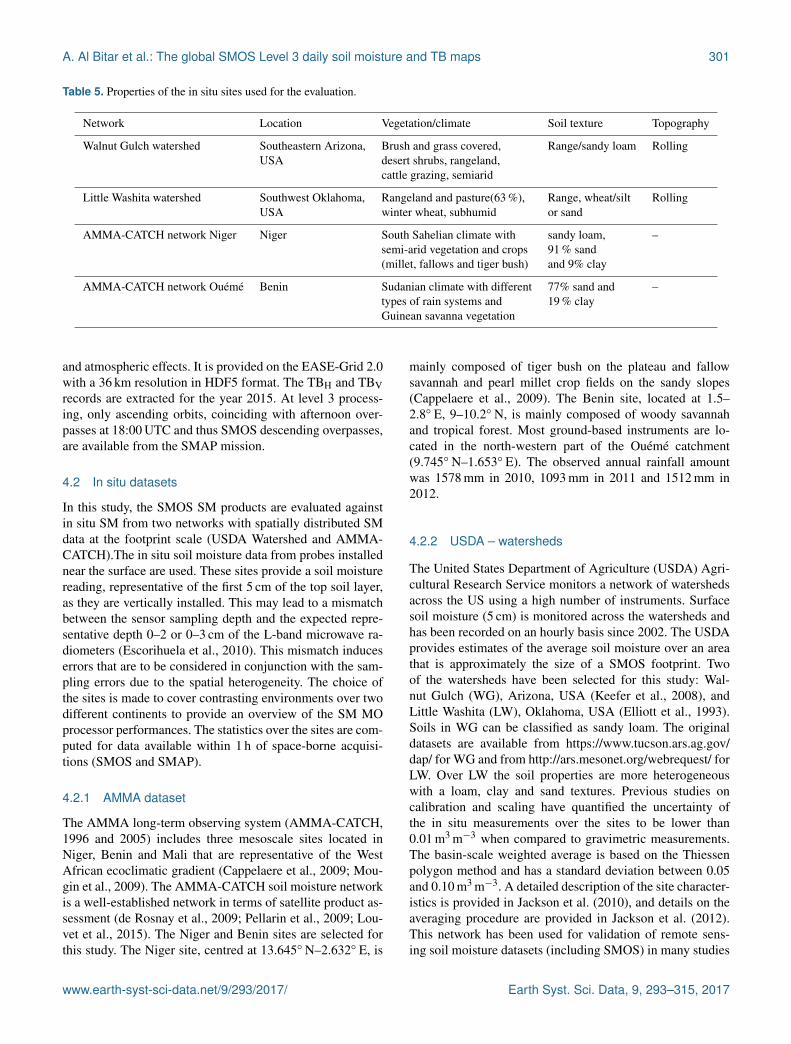
Table 5. Properties of the in situ sites used for the evaluation.

Network Location Vegetation/climate Soil texture Topography

Walnut Gulch watershed Southeastern Arizona, Brush and grass covered, Range/sandy loam RollingUSA desert shrubs, rangeland,

cattle grazing, semiarid

Little Washita watershed Southwest Oklahoma, Rangeland and pasture(63 %), Range, wheat/silt RollingUSA winter wheat, subhumid or sand

AMMA-CATCH network Niger Niger South Sahelian climate with sandy loam, –semi-arid vegetation and crops 91 % sand(millet, fallows and tiger bush) and 9% clay

AMMA-CATCH network Ouémé Benin Sudanian climate with different 77% sand and –types of rain systems and 19 % clayGuinean savanna vegetation

and atmospheric effects. It is provided on the EASE-Grid 2.0with a 36 km resolution in HDF5 format. The TBH and TBVrecords are extracted for the year 2015. At level 3 process-ing, only ascending orbits, coinciding with afternoon over-passes at 18:00 UTC and thus SMOS descending overpasses,are available from the SMAP mission.

4.2 In situ datasets

In this study, the SMOS SM products are evaluated againstin situ SM from two networks with spatially distributed SMdata at the footprint scale (USDA Watershed and AMMA-CATCH).The in situ soil moisture data from probes installednear the surface are used. These sites provide a soil moisturereading, representative of the first 5 cm of the top soil layer,as they are vertically installed. This may lead to a mismatchbetween the sensor sampling depth and the expected repre-sentative depth 0–2 or 0–3 cm of the L-band microwave ra-diometers (Escorihuela et al., 2010). This mismatch induceserrors that are to be considered in conjunction with the sam-pling errors due to the spatial heterogeneity. The choice ofthe sites is made to cover contrasting environments over twodifferent continents to provide an overview of the SM MOprocessor performances. The statistics over the sites are com-puted for data available within 1 h of space-borne acquisi-tions (SMOS and SMAP).

4.2.1 AMMA dataset

The AMMA long-term observing system (AMMA-CATCH,1996 and 2005) includes three mesoscale sites located inNiger, Benin and Mali that are representative of the WestAfrican ecoclimatic gradient (Cappelaere et al., 2009; Mou-gin et al., 2009). The AMMA-CATCH soil moisture networkis a well-established network in terms of satellite product as-sessment (de Rosnay et al., 2009; Pellarin et al., 2009; Lou-vet et al., 2015). The Niger and Benin sites are selected forthis study. The Niger site, centred at 13.645◦ N–2.632◦ E, is

mainly composed of tiger bush on the plateau and fallowsavannah and pearl millet crop fields on the sandy slopes(Cappelaere et al., 2009). The Benin site, located at 1.5–2.8◦ E, 9–10.2◦ N, is mainly composed of woody savannahand tropical forest. Most ground-based instruments are lo-cated in the north-western part of the Ouémé catchment(9.745◦ N–1.653◦ E). The observed annual rainfall amountwas 1578 mm in 2010, 1093 mm in 2011 and 1512 mm in2012.

4.2.2 USDA – watersheds

The United States Department of Agriculture (USDA) Agri-cultural Research Service monitors a network of watershedsacross the US using a high number of instruments. Surfacesoil moisture (5 cm) is monitored across the watersheds andhas been recorded on an hourly basis since 2002. The USDAprovides estimates of the average soil moisture over an areathat is approximately the size of a SMOS footprint. Twoof the watersheds have been selected for this study: Wal-nut Gulch (WG), Arizona, USA (Keefer et al., 2008), andLittle Washita (LW), Oklahoma, USA (Elliott et al., 1993).Soils in WG can be classified as sandy loam. The originaldatasets are available from https://www.tucson.ars.ag.gov/dap/ for WG and from http://ars.mesonet.org/webrequest/ forLW. Over LW the soil properties are more heterogeneouswith a loam, clay and sand textures. Previous studies oncalibration and scaling have quantified the uncertainty ofthe in situ measurements over the sites to be lower than0.01 m3 m−3 when compared to gravimetric measurements.The basin-scale weighted average is based on the Thiessenpolygon method and has a standard deviation between 0.05and 0.10 m3 m−3. A detailed description of the site character-istics is provided in Jackson et al. (2010), and details on theaveraging procedure are provided in Jackson et al. (2012).This network has been used for validation of remote sens-ing soil moisture datasets (including SMOS) in many studies


https://www.tucson.ars.ag.gov/dap/

https://www.tucson.ars.ag.gov/dap/

http://ars.mesonet.org/webrequest/


(Sahoo et al., 2008; Jackson et al., 2012; Leroux et al., 2014).Information on land use and topography of these sites is pro-vided in Table 5.

5 Methodology of evaluation

5.1 Global comparison of SMOS and SMAP TB

In order to compare the SMOS TB product to SMAP TB,the SMOS daily product was averaged following the sameinterpolation procedure as the one suggested in the SMAPmission. The method consists of using an inverse distanceweighting for all the SMOS EASE 2.0 25 km grid points atthe limits of the EASE 2.0 36 km grid of the SMAP prod-uct. The TBH and TBV from SMAP products are extractedand used without modification. The comparison is done overthe pixels with a water fraction of less than 0.01 (i.e. 1 %)since the SMAP TBs are provided with subtracted open sur-face water. The contribution of the water surface is computedconsidering surface fraction from MODIS MOD44W andthe emission of water using the Klein–Swift (1977) dielec-tric constant model forced by the surface soil layer temper-ature from GSFC (Goddard Space Flight Center) (O’Neil etal., 2015).

5.2 Global soil moisture maps comparison

Global comparison is done over the EASE-Grid 2.0 25 kmused for the L3 MO SM product. The L3 MO SM field is ex-tracted directly from the product. The L2 SO SM product isinterpolated to the EASE-Grid 2.0 25 km using a three-stageinterpolation strategy where the availability of the productsinside the limits of the grid node is considered

– bilinear, if more than two soil moisture retrievals areavailable;

– linear, if two soil moisture retrievals are available;

– nearest point, if one soil moisture retrieval is available.

The L2 SO SM is also filtered at high latitude where severalsoil moisture retrievals are available. The selection criterionis minimum distance from the swath centre, the same as forthe L3 MO SM algorithm.

5.3 Local evaluations

No interpolation is used after the extraction of the SM timeseries. The comparison is based on the following statisticalindicators:

– mean bias: (in situ – retrieved soil moisture) (m3 m−3)

– standard error of the estimate (SEE) (m3 m−3)

– Pearson correlation coefficient (R)

– RMSE (m3 m−3)

– the empirical cumulative distribution function (Cox andOakes, 1984).

6 Results and discussions

6.1 SMOS and SMAP brightness temperatures

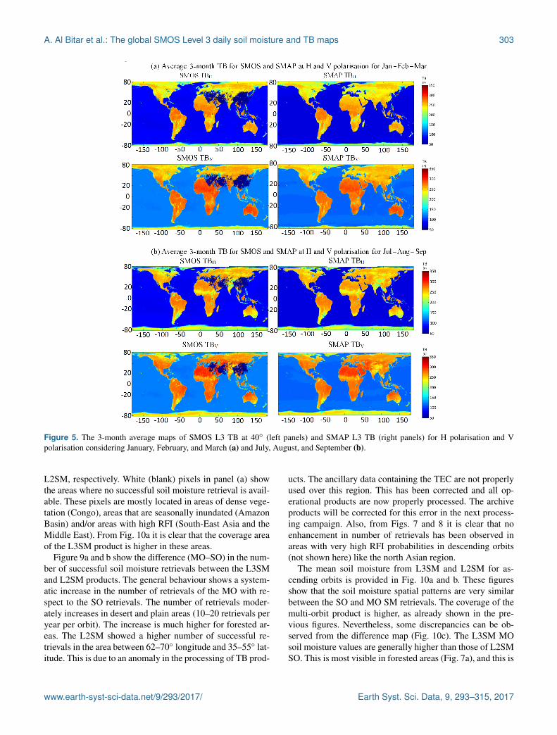
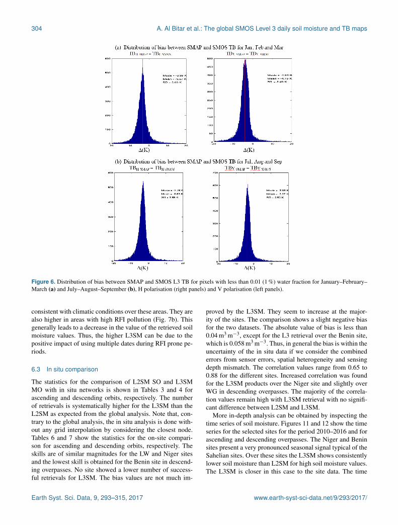
Figures 5a, b and 6a, b show the comparison between theSMOS L3 TB and SMAP L3 TB at a 40◦ incidence an-gle. Figure 5a shows the average of SMOS and SMAP TBHand TBV for the winter (January, February and March) andsummer (July, August and September) seasons for 2016. Thegaps (in dark blue) in the SMOS images are due to RFI witha differentiated impact for ascending and descending orbits.The difference in TBs between H/V acquisitions is smallerthan between ascending and descending configurations. Themain explanations for these differences are that, first, the L1algorithm in SMOS and SMAP does not use the same con-figuration for the computation of the Faraday rotation. TheFaraday rotation is impacted by the TEC (total electroniccontent) in the ionosphere. The SMAP algorithm uses theSTOKES 3 parameters to account for the Faraday rotation.The SMOS algorithm uses auxiliary TEC files to computethe Faraday rotation. The ionosphere TEC is very differentbetween ascending and descending orbits as the heating dur-ing the day increases the TEC. The second explanation isthat the RFI probabilities are very different between ascend-ing and descending orbits due to directional aspects and theyare closer between H/V polarisations. The SMAP productsshow a higher coverage because SMAP has on-board RFI fil-tering and mitigation, which enables a better coverage but atthe cost of a lower radiometric accuracy. The spatial patternsof TB are highly consistent for the two missions. Figure 6aand b show the distribution of difference of TBH and TBVfrom SMOS and SMAP for the winter (January, Februaryand March) and summer (July, August and September) sea-sons during 2016. As described in Sect. 5.1, only nodes witha water fraction of less than 0.01 (i.e. 1 %) are considered.The mean difference is about−3.67 to−4.16 K, with SMAPbeing colder independent of polarisation or season. The stan-dard deviation of all comparisons is about 3.65 K. This valueis due to differences in calibration of the sensors and to theimpact of differences in the acquisition time.

6.2 Soil moisture retrievals on a global scale

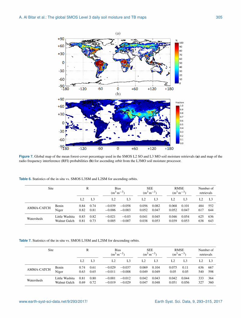
Based on the aforementioned evaluation methodology, theL3SM MO retrievals are compared to those of L2SM SO onthe global scale over the 2010–2015 period. The auxiliarymaps of mean forest cover percentage (Fig. 7a) and averageRFI probabilities (Fig. 7b) for 2011 are provided as com-plementary information. These maps are obtained from theL3SM product.

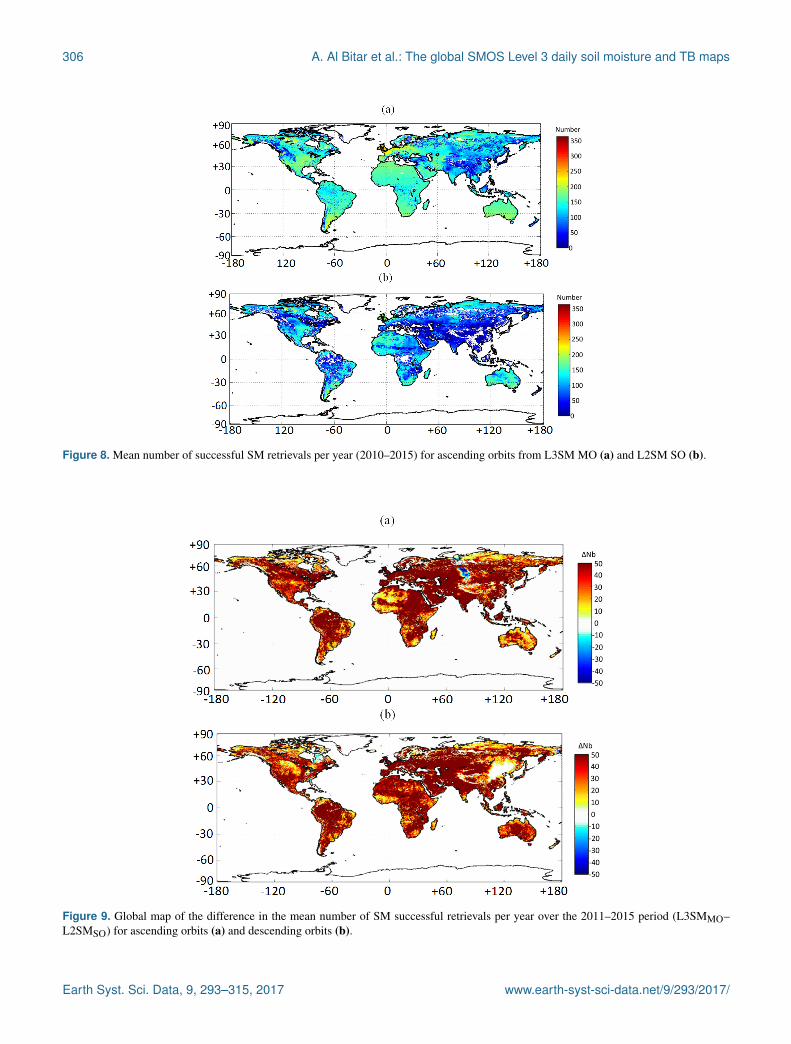
Figure 8a and b show the mean number of successfulretrievals per year (2010–2015) obtained from L3SM and



Figure 5. The 3-month average maps of SMOS L3 TB at 40◦ (left panels) and SMAP L3 TB (right panels) for H polarisation and Vpolarisation considering January, February, and March (a) and July, August, and September (b).

L2SM, respectively. White (blank) pixels in panel (a) showthe areas where no successful soil moisture retrieval is avail-able. These pixels are mostly located in areas of dense vege-tation (Congo), areas that are seasonally inundated (AmazonBasin) and/or areas with high RFI (South-East Asia and theMiddle East). From Fig. 10a it is clear that the coverage areaof the L3SM product is higher in these areas.

Figure 9a and b show the difference (MO–SO) in the num-ber of successful soil moisture retrievals between the L3SMand L2SM products. The general behaviour shows a system-atic increase in the number of retrievals of the MO with re-spect to the SO retrievals. The number of retrievals moder-ately increases in desert and plain areas (10–20 retrievals peryear per orbit). The increase is much higher for forested ar-eas. The L2SM showed a higher number of successful re-trievals in the area between 62–70◦ longitude and 35–55◦ lat-itude. This is due to an anomaly in the processing of TB prod-

ucts. The ancillary data containing the TEC are not properlyused over this region. This has been corrected and all op-erational products are now properly processed. The archiveproducts will be corrected for this error in the next process-ing campaign. Also, from Figs. 7 and 8 it is clear that noenhancement in number of retrievals has been observed inareas with very high RFI probabilities in descending orbits(not shown here) like the north Asian region.

The mean soil moisture from L3SM and L2SM for as-cending orbits is provided in Fig. 10a and b. These figuresshow that the soil moisture spatial patterns are very similarbetween the SO and MO SM retrievals. The coverage of themulti-orbit product is higher, as already shown in the pre-vious figures. Nevertheless, some discrepancies can be ob-served from the difference map (Fig. 10c). The L3SM MOsoil moisture values are generally higher than those of L2SMSO. This is most visible in forested areas (Fig. 7a), and this is



Figure 6. Distribution of bias between SMAP and SMOS L3 TB for pixels with less than 0.01 (1 %) water fraction for January–February–March (a) and July–August–September (b), H polarisation (right panels) and V polarisation (left panels).

consistent with climatic conditions over these areas. They arealso higher in areas with high RFI pollution (Fig. 7b). Thisgenerally leads to a decrease in the value of the retrieved soilmoisture values. Thus, the higher L3SM can be due to thepositive impact of using multiple dates during RFI prone pe-riods.

6.3 In situ comparison

The statistics for the comparison of L2SM SO and L3SMMO with in situ networks is shown in Tables 3 and 4 forascending and descending orbits, respectively. The numberof retrievals is systematically higher for the L3SM than theL2SM as expected from the global analysis. Note that, con-trary to the global analysis, the in situ analysis is done with-out any grid interpolation by considering the closest node.Tables 6 and 7 show the statistics for the on-site compari-son for ascending and descending orbits, respectively. Theskills are of similar magnitudes for the LW and Niger sitesand the lowest skill is obtained for the Benin site in descend-ing overpasses. No site showed a lower number of success-ful retrievals for L3SM. The bias values are not much im-

proved by the L3SM. They seem to increase at the major-ity of the sites. The comparison shows a slight negative biasfor the two datasets. The absolute value of bias is less than0.04 m3 m−3, except for the L3 retrieval over the Benin site,which is 0.058 m3 m−3. Thus, in general the bias is within theuncertainty of the in situ data if we consider the combinederrors from sensor errors, spatial heterogeneity and sensingdepth mismatch. The correlation values range from 0.65 to0.88 for the different sites. Increased correlation was foundfor the L3SM products over the Niger site and slightly overWG in descending overpasses. The majority of the correla-tion values remain high with L3SM retrieval with no signifi-cant difference between L2SM and L3SM.

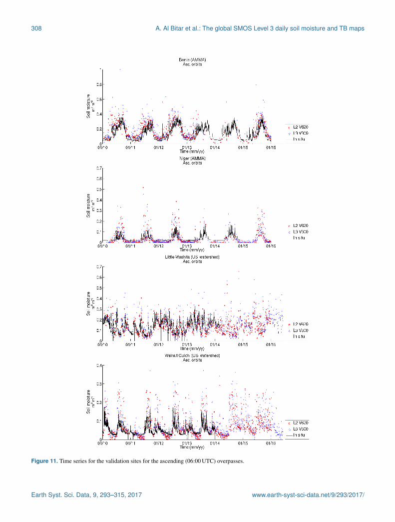
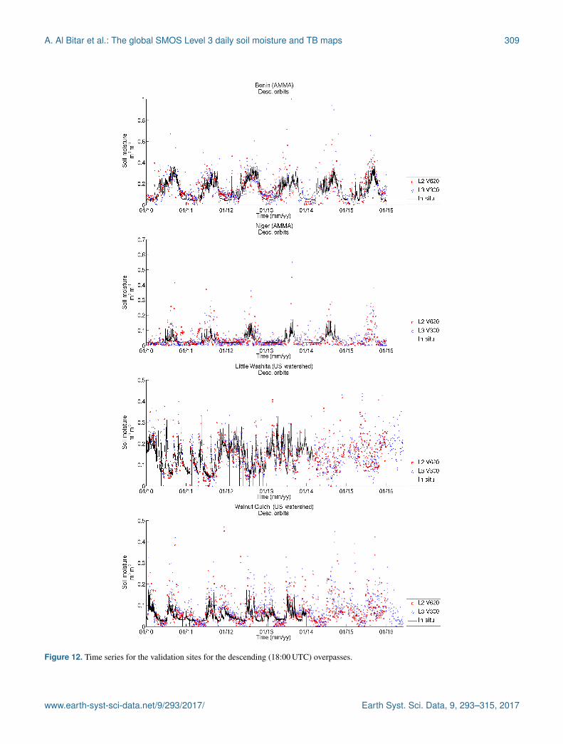
More in-depth analysis can be obtained by inspecting thetime series of soil moisture. Figures 11 and 12 show the timeseries for the selected sites for the period 2010–2016 and forascending and descending overpasses. The Niger and Beninsites present a very pronounced seasonal signal typical of theSahelian sites. Over these sites the L3SM shows consistentlylower soil moisture than L2SM for high soil moisture values.The L3SM is closer in this case to the site data. The time



Figure 7. Global map of the mean forest-cover percentage used in the SMOS L2 SO and L3 MO soil moisture retrievals (a) and map of theradio frequency interference (RFI) probabilities (b) for ascending orbit from the L3MO soil moisture processor.

Table 6. Statistics of the in situ vs. SMOS L3SM and L2SM for ascending orbits.

Site R Bias SEE RMSE Number of(m3 m−3) (m3 m−3) (m3 m−3) retrievals

L2 L3 L2 L3 L2 L3 L2 L3 L2 L3

AMMA-CATCHBenin 0.84 0.74 −0.039 −0.058 0.056 0.082 0.068 0.101 484 552Niger 0.82 0.81 −0.006 −0.003 0.052 0.047 0.052 0.047 617 644

WatershedsLittle Washita 0.83 0.82 −0.021 −0.03 0.041 0.045 0.046 0.054 625 636Walnut Gulch 0.81 0.73 0.005 −0.007 0.038 0.053 0.039 0.053 638 643

Table 7. Statistics of the in situ vs. SMOS L3SM and L2SM for descending orbits.

Site R Bias SEE RMSE Number of(m3 m−3) (m3 m−3) (m3 m−3) retrievals

L2 L3 L2 L3 L2 L3 L2 L3 L2 L3

AMMA-CATCHBenin 0.74 0.61 −0.029 −0.037 0.069 0.104 0.075 0.11 636 667Niger 0.63 0.65 −0.011 −0.008 0.049 0.049 0.05 0.05 540 598

WatershedsLittle Washita 0.81 0.80 −0.001 −0.012 0.042 0.043 0.042 0.044 333 364Walnut Gulch 0.69 0.72 −0.019 −0.029 0.047 0.048 0.051 0.056 327 360



Figure 8. Mean number of successful SM retrievals per year (2010–2015) for ascending orbits from L3SM MO (a) and L2SM SO (b).

Figure 9. Global map of the difference in the mean number of SM successful retrievals per year over the 2011–2015 period (L3SMMO–L2SMSO) for ascending orbits (a) and descending orbits (b).



Figure 10. Mean soil moisture map over 2011–2015 for ascending orbits from CATDS L3SM MO (a), DPGS L2SM SO (b) and thedifference (MO–SO) map between L3SM MO and L2SM SO (c).

series for LW show that the SMOS data closely follow thebehaviour of the soil moisture dynamics over this site. Oneof the reasons for this is that the rainfall events are well sepa-rated, enabling the remote sensing data to capture the dynam-ics of physical processes (e.g. infiltration and evaporation) ona coarse scale. Thus, the exponential behaviour typical of adrying soil is well depicted.

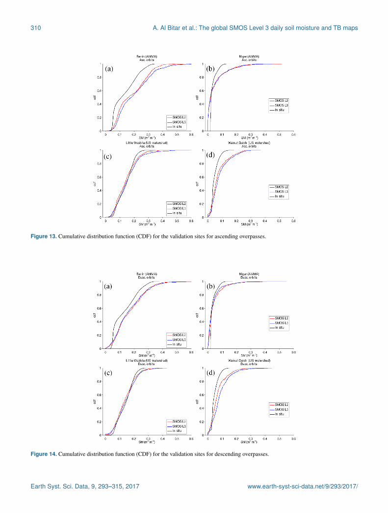
Figures 13 and 14 show the CDF of the in situ, L2SM andL3SM data for ascending and descending orbits. From thesefigures it can be concluded that the SMOS soil moisture isdrier than the 5 cm in situ data across the different valuesof soil moisture. This can be explained by the SMOS pene-tration depth with respect to the depth of the installation of

the in situ sensors. Nevertheless, the shape of the distributionfunction, describing the extreme and seasonal cycles, is wellcaptured in most cases. The Niger site’s Sahelian climate iswell captured, with a high probability of low soil moisturevalues and a small number of extreme values. The differencesbetween the L2SM and L3SM data are mainly observed forthe Benin and LW sites. When comparing Figs. 13 and 14,small differences can be noted between ascending and de-scending orbits.



Figure 11. Time series for the validation sites for the ascending (06:00 UTC) overpasses.



Figure 12. Time series for the validation sites for the descending (18:00 UTC) overpasses.



Figure 13. Cumulative distribution function (CDF) for the validation sites for ascending overpasses.

Figure 14. Cumulative distribution function (CDF) for the validation sites for descending overpasses.



7 Data availability

The main datasets can be accessed as follows:

– MIR_CLF31A / D: SMOS-CATDS Level 3 1-daysoil moisture maps for ascending (06:00 UTC) anddescending (18:00 UTC) orbits version 300, link:ftp://[email protected]/Land_products/GRIDDED/L3SM/RE04/MIR_CLF31A/;

– MIR_CDF3TA / D: SMOS-CATDS Level 3 1-dayfixed-angle bin full-polarisation brightness tem-peratures maps for ascending (06:00 UTC) anddescending (18H00) orbits version 310, link:ftp://[email protected]/Land_products/GRIDDED/L3SM/RE04/MIR_CLF31A/.

8 Conclusions

The level 3 daily maps of soil moisture and brightness tem-peratures are presented in this paper. A multi-orbit soil mois-ture retrieval algorithm for SMOS data is used to obtain thesoil moisture product. The main feature of the algorithm isthe use of MO and of temporal autocorrelation of opticalvegetation depth in the cost function. The algorithm is im-plemented operationally at CATDS. The processing chaindelivers gridded products over the EASE 2.0 grid at 25 kmin netCDF format. The L3 angle-binned TB product is com-pared to SMAP brightness temperature maps at 40◦. The re-sults show small differences in mean TB between the prod-ucts for H/V polarisation and ascending and descending or-bits. The SMAP product presents a wider coverage due to theon-board RFI filtering. The L3SM MO product is comparedto the L2SM SO product. The best improvements in algo-rithm performances are in terms of the number of successfulretrievals observed over forested and RFI-prone areas. Also,the L3SM MO product shows, on average, wetter soil mois-ture retrievals than the L2SM SO. The comparison with lo-cal sites showed that the quality of the retrievals is compara-ble between L2SM SO and L3SM MO. This shows that theincrease in the number of successful retrievals does not de-grade quality, but rather comes at the expense of an increasedtime lag in product availability (6 h for L2SM SO versus 3.5to 7 days for L3SM MO). The SO and MO products showa slight dry bias except for the AMMA Benin site, whichis smaller than the in situ data uncertainty (< 0.04 m3 m−3).More accurate auxiliary files like soil maps from SoilGrids(https://www.soilgrids.org/) may improve the retrieval qual-ity, but more densely instrumented sites will be needed toaccess the improvements. Future works will concentrate onthe associated optical depth product not presented in this pa-per. An application of the algorithm to the SMAP data hasbeen envisioned.


ftp://[email protected]/Land_products/GRIDDED/L3SM/RE04/MIR_CLF31A/




https://www.soilgrids.org/


Appendix A: List of abbreviations

ARS Agricultural Research ServiceAMMA Analyse Multidisciplinaire de la MoussonAMSR-E Advanced Microwave Scanning Radiometer – Earth Observing SystemASCAT Advanced ScatterometerCATDS Centre Aval de Traitement des Données SMOSCNES Centre National d’Etudes SpatialesCCI Climate Change InitiativeCDTI Centro para el Desarrollo Tecnológico IndustrialDPGS Data Processing Ground SegmentEASE-Grid Equal-Area Scalable Earth GridECMWF European Centre for Medium-Range Weather ForecastsECV Essential Climate VariablesEO Earth observationESA European Space AgencyIFREMER Institut Français de Recherche pour l’Exploitation de la MerISEA Icosahedral Snyder Equal AreaL-MEB L-band Microwave Emission of the BiosphereMO Multi OrbitMODIS Moderate-Resolution Imaging SpectroradiometerNASA National Aeronautics and Space Administration (USA)SM Soil MoistureSMAP Soil Moisture Active PassiveSMOS Soil Moisture and Ocean SalinitySMUDP Soil Moisture User Data ProductSO Single OrbitTOA Top of AtmosphereUSDA United States Department of AgricultureVOD Vegetation Optical DepthERS European Remote SensingATBD Algorithm Theoretical Basis DocumentNSIDC National Snow and Ice Data Center (USA)GSFC Goddard Space Flight CenterUTC Coordinated Universal Time



Competing interests. The authors declare that they have no con-flict of interest.

Acknowledgements. The SMOS L3SM products were obtainedfrom the Centre Aval de Traitement des Données SMOS (CATDS),operated for the “Centre National d’Etudes Spatiales” (CNES,France) by IFREMER (Brest, France). This study was supportedby the CNES “Terre, Océan, Surfaces Continentales, Atmosphère”program. The authors would like to thank the USDA ARS Hydrol-ogy and Remote Sensing Laboratory, AMMA-CATCH project forthe in situ datasets.

Edited by: D. CarlsonReviewed by: M. Schwank and one anonymous referee

References

Al Bitar, A., Leroux, D. J., Kerr, Y. H., Merlin, O., Richaume, P.,Sahoo, A., and Wood, E. F.: Evaluation of SMOS Soil MoistureProducts Over Continental U.S. Using the SCAN/SNOTEL Net-work, IEEE T. Geosci. Remote, 50, 1572–1586, 2012.

Al-Yaari, A., Wigneron, J. P., Ducharne, A., Kerr, Y., de Rosnay, P.,de Jeu, R., Govind, A., Al Bitar, A., Albergel, C., Muñoz-Sabater,J., Richaume, P., and Mialon, A.: Global-scale evaluation of twosatellite-based passive microwave soil moisture datasets (SMOSand AMSR-E) with respect to Land Data Assimilation Systemestimates, Remote Sens. Environ., 149, 181–195, 2014a.

Al-Yaari, A., Wigneron, J. P., Ducharne, A., Kerr, Y. H., Wag-ner, W., De Lannoy, G., Reichle, R., Al Bitar, A., Dorigo, W.,Richaume, P., and Mialon, A.: Global-scale comparison of pas-sive (SMOS) and active (ASCAT) satellite based microwavesoil moisture retrievals with soil moisture simulations (MERRA-Land), Remote Sens. Environ., 152, 614–626, 2014b.

AMMA-CATCH: Rivers flow and water electrical conductivity,Oueme meso site, Benin, IRD, CNRS-INSU, OSUG, OMP,OREME, https://doi.org/10.5072/AMMA-CATCH.CL.Run_O,1996.

AMMA-CATCH: Surface energy, water vapor, and carbonfluxes, Wankama local site, Niger, IRD, CNRS-INSU,OSUG, OMP, OREME. https://doi.org/10.5072/AMMA-CATCH.AE.H2OFlux_Ncw, 2005.

Brocca, L., Melone, F., Moramarco, T., Wagner, W., Naeimi,V., Bartalis, Z., and Hasenauer, S.: Improving runoff pre-diction through the assimilation of the ASCAT soil mois-ture product, Hydrol. Earth Syst. Sci., 14, 1881–1893,https://doi.org/10.5194/hess-14-1881-2010, 2010.

Brodzik, M. J. and Knowles, K. W.: EASE-Grid: A Versatile Setof Equal-Area Projections and Grids, in: Discrete Global Grids,edited by: Goodchild, M. and Kimerling, A. J., National Centerfor Geographic Information & Analysis, Santa Barbara, Califor-nia USA, 2002.

Cappelaere, B., Descroix, L., Lebel, T., Boulain, N., Ramier,D., Laurent, J.-P., Favreau, G., Boubkraoui, S., Boucher, M.,Moussa, I. B., Chaffard, V., Hiernaux, P., Issoufou, H. B. A.,Le Breton, E., Mamadou, I., Nazoumou, Y., Oï, M., Ottlé, C.,and Quantin, G.: The AMMA-CATCH experiment in the culti-vated Sahelian area of south-west Niger – Investigating water cy-

cle response to a fluctuating climate and changing environment,J. Hydrol., 375, 34–51, 2009.

Carr, D. B., Kahn, R., Sahr, K., and Olsen, T.: ISEA Discrete GlobalGrids, Statistical Computing & Statistical Graphics Newsletter,8, 31–39, 1997.

Cox, D. R. and Oakes, D.: Analysis of Survival Data, Chapman &Hall, London, UK, 1984.

de Rosnay, P., Gruhier, C., Timouk, F., Baup, F., Mougin, E., Hier-naux, P., Kergoat, L., and LeDantec, V.: Multiscale soil moisturemeasurements at the Gourma meso-scale site in Mali, J. Hydrol.,375, 241–252, 2009.

de Rosnay, P., Drusch, M., Vasiljevic, D., Balsamo, G., Albergel,C., and Isaksen, L.: A simplified Extended Kalman Filter for theglobal operational soil moisture analysis at ECMWF, Q. J. Roy.Meteor. Soc., 139, 1199–1213, 2013.

Drusch, M.: Initializing numerical weather prediction models withsatellite-derived surface soil moisture: Data assimilation ex-periments with ECMWF’s integrated forecast system and theTMI soil moisture data set, J. Geophys. Res., 112, D03102,https://doi.org/10.1029/2006JD007478, 2007.

Elliott, R. L., Schiebe, F. R., Crawford, K. C., Peter, K. D., andPuckett, W. E.: A Unique Data Capability for Natural Re-sources Studies, International Winter Meeting; American Societyof Agricultural Engineers, Chicago, IL, 14–17 December 1993,ASAE Paper No. 932529, 1993.

Entekhabi, D., Njoku, E. G., O’Neill, P. E., Kellogg, K. H., Crow,W. T., Edelstein, W. N., Entin, J. K., Goodman, S. D., Jackson,T. J., Johnson, J., Kimball, J., Piepmeier, J. R., Koster, R. D.,Martin, N., McDonald, K. C., Moghaddam, M., Moran, S., Re-ichle, R., Shi, J. C., Spencer, M. W., Thurman, S. W., Tsang, L.,and Zyl, J. V.: The Soil Moisture Active Passive (SMAP) Mis-sion, Proceedings of the IEEE, 98, 704–716, 2010.

Escorihuela, M. J., Chanzy, A., Wigneron, J. P., and Kerr, Y. H.:Effective soil moisture sampling depth of L-band radiometry: Acase study, Remote Sens. Environ., 114, 995–1001, 2010.

Guérif, M. and Duke, C. L.: Adjustment procedures of a crop modelto the site specific characteristics of soil and crop using remotesensing data assimilation, Agr. Ecosyst. Environ., 81, 57–69,https://doi.org/10.1016/S0167-8809(00)00168-7, 2000.

Hagolle, O., Dedieu, G., Mougenot, B., Debaecker, V., Duchemin,B., and Meygret, A.: Correction of aerosol effects on multi-temporal images acquired with constant viewing angles: Appli-cation to Formosat-2 images, Remote Sens. Environ., 112, 1689–1701, 2008.

Hagolle, O., Huc, M., Pascual, D. V., Dedieu, G.: A multi-temporalmethod for cloud detection, applied to FORMOSAT-2, VENµS,LANDSAT and SENTINEL-2 images, Remote Sens. Environ.,114, 1747–1755, 2010.

Hagolle, O., Huc, M., Villa Pascual, D., and Dedieu, G.: A Multi-Temporal and Multi-Spectral Method to Estimate Aerosol Op-tical Thickness over Land, for the Atmospheric Correction ofFormoSat-2, LandSat, VENµS and Sentinel-2 Images, RemoteSensing, 7, 2668–2691, 2015.

Hollmann, R., Merchant, C. J., Saunders, R., Downy, C., Buch-witz, M., Cazenave, A., Chuvieco, E., Defourny, P., de Leeuw,G., Forsberg, R., Holzer-Popp, T., Paul, F., Sandven, S., Sathyen-dranath, S., van Roozendael, M., and Wagner, W.: The ESA cli-mate change initiative: Satellite data records for essential climatevariables, B. Am. Meteorol. Soc., 94, 1541–1552, 2013.


https://doi.org/10.5072/AMMA-CATCH.CL.Run_O

https://doi.org/10.5072/AMMA-CATCH.AE.H2OFlux_Ncw

https://doi.org/10.5072/AMMA-CATCH.AE.H2OFlux_Ncw

https://doi.org/10.5194/hess-14-1881-2010

https://doi.org/10.1029/2006JD007478

https://doi.org/10.1016/S0167-8809(00)00168-7


Inglada, J. and Mercier, G.: A new statistical similarity measure forchange detection in multitemporal SAR images and its exten-sion to multiscale change analysis, IEEE T. Geosci. Remote, 45,1432–1445, 2007.

Jackson, T. J. and Schmugge, T. J.: Vegetation effects on the mi-crowave emission of soils, Remote Sens. Environ., 36, 203–212,1991.

Jackson, T. J., Cosh, M. H., Bindlish, R., Starks, P. J., Bosch, D. D.,Seyfried, M., Goodrich, D. C., Moran, M. S., and Du, J.: Valida-tion of Advanced Microwave Scanning Radiometer soil moistureproducts, IEEE T. Geosci. Remote, 48, 4256–4272, 2010.

Jackson, T. J., Bindlish, R., Cosh, M., Zhao, T., Starks, P., Bosch,D., Seyfried, M., Moran, M. S., Goodrich, D., Kerr, Y. H.,and Leroux, D.: Validation of Soil Moisture and Ocean Salin-ity (SMOS) Soil Moisture Over Watershed Networks in the U.S.,IEEE T. Geosci. Remote, 50, 1530–1543, 2012.

Jung, M., Reichstein, M., Ciais, P., Seneviratne, S. I., Sheffield,J., Goulden, M. L., Bonan, G., Cescatti, A., Chen, J., de Jeu,R., Dolman, A. J., Eugster, W., Gerten, D., Gianelle, D., Go-bron, N., Heinke, J., Kimball, J., Law, B. E., Montagnani, L.,Mu, Q., Mueller, B., Oleson, K., Papale, D., Richardson, A. D.,Roupsard, O., Running, S., Tomelleri, E., Viovy, N., Weber, U.,Williams, C., Wood, E., Zaehle, S., and Zhang, K.: Recent de-cline in the global land evapotranspiration trend due to limitedmoisture supply, Nature, 467, 951–954, 2010.

Keefer, T. O., Moran, M. S., and Paige, G. B.: Long-term meteoro-logical and soil hydrology database, Walnut Gulch Experimen-tal Watershed, Arizona, United States, Water Resour. Res., 44,W05S07, https://doi.org/10.1029/2006WR005702, 2008.

Kerr, Y. H. and Njoku, E. G.: Semiempirical model for in-terpreting microwave emission from semiarid land surfacesas seen from space, IEEE T. Geosci. Remote, 28, 384–393,https://doi.org/10.1109/36.54364, 1990.

Kerr, Y. H., Waldteufel, P., Wigneron, J.-P., Martinuzzi, J. M., Font,J., and Berger, M.: Soil moisture retrieval from space: The SoilMoisture and Ocean Salinity (SMOS) mission, IEEE T. Geosci.Remote, 39, 1729–1735, https://doi.org/10.1109/36.942551,2001.

Kerr, Y. H., Waldteufel, P., Wigneron, J.-P., Delwart, S.,Cabot, F., Boutin, J., Escorihuela, M. J., Font, J., Reul,N., Gruhier, C., Juglea, S. E., Drinkwater, M. R., Hahne,A., Martin-Neira, M., and Mecklenburg, S.: The SMOSMission: New Tool for Monitoring Key Elements of theGlobal Water Cycle, Proceedings of the IEEE, 98, 666–687,https://doi.org/10.1109/JPROC.2010.2043032, 2010.

Kerr, Y. H., Waldteufel, P., Richaume, P., Wigneron, J.-P., Ferraz-zoli, P., Mahmoodi, A., Al Bitar, A., Cabot, F., Gruhier, C.,Enache Juglea, S., Leroux, D., Mialon, A., and Delwart, S.: TheSMOS Soil Moisture Retrieval Algorithm, IEEE T. Geosci. Re-mote, 50, 1384–1403, 2012.

Kerr, Y. H., Jacquette, E., Al Bitar, A., Cabot, F., Mialon, A.,and Richaume, P.: CATDS SMOS L3 soil moisture retrievalprocessor, Algorithm Theoretical Baseline Document (ATBD),CATDS, 73 pp., 2013.

Keyantash, J. and Dracup, J. A.: The quantification of drought: anevaluation of drought indices, B. Am. Meteorol. Soc., 83, 1167–1180, 2002.

Khazâal, A., Anterrieu, E., Cabot, F., and Kerr, Y. H.: Impact of Di-rect Solar Radiations Seen by the Back-Lobes Antenna Patterns

of SMOS on the Retrieved Images, IEEE J. Sel. Top. Appl., PP,1–8, https://doi.org/10.1109/JSTARS.2016.2609601, 2016.

Klein, L. A. and Swift, C. T.: An Improved Model for the Di-electric Constant of Sea Water at Microwave Frequencies, IEEEJ. Oceanic Eng., 2, 104–111, 1977.

Konings, A. G., Piles, M., Rötzer, K., McColl, K. A., Chan, S. K.,and Entekhabi, D.: Vegetation optical depth and scattering albedoretrieval using time series of dual-polarized L-band radiometerobservations, Remote Sens. Environ., 172, 178–189, 2016.

Koster, R. D., Dirmeyer, P. A., Guo, Z., Bonan, G., Chan, E., Cox,P., Gordon, C. T., Kanae, S., Kowalczyk, E., Lawrence, D., Liu,P., Lu, C.-H., Malyshev, S., McAvaney, B., Mitchell, K., Mocko,D., Oki, T., Oleson, K., Pitman, A., Sud, Y. C., Taylor, C. M.,Verseghy, D., Vasic, R., Xue, Y., and Yamada, T.: Regions ofstrong coupling between soil moisture and precipitation, Science,305, 1138–1140, 2004.

Leroux, D. J., Kerr, Y. H., Al Bitar, A., Bindlish, R., Jackson, T.,Berthelot, B., and Portet, G.: Comparison Between SMOS, VUA,ASCAT, and ECMWF Soil Moisture Products Over Four Water-sheds in U.S., IEEE T. Geosci. Remote, 52, 1562–1571, 2014.

Lievens, H., Tomer, S. K., Al Bitar, A., De Lannoy, G. J. M., Drusch,M., Dumedah, G., Franssen, H. J. H., Kerr, Y. H., Martens, B.,Pan, M., and Roundy, J. K.: SMOS soil moisture assimilationfor improved hydrologic simulation in the Murray Darling Basin,Australia, Remote Sens. Environ., 168, 146–162, 2015.

Liu, S. F., Liou, Y.-A., Wang, W. J., Wigneron, J.-P., and Lee, J. B.:Retrieval of crop biomass and soil moisture from measured 1.4and 10.65 brightness temperatures, IEEE T. Geosci. Remote, 40,1260–1268, 2002.

Louvet, S., Pellarin, T., Al Bitar, A., Cappelaere, B., Galle, S.,Grippa, M., Gruhier, C., Kerr, Y., Lebel, T., Mialon, A., Mou-gin, E., Quantin, G., Richaume, P., and de Rosnay, P.: SMOSsoil moisture product evaluation over West-Africa from lo-cal to regional scale, Remote Sens. Environ., 156, 383–394,https://doi.org/10.1016/j.rse.2014.10.005, 2015.

Masson, V., Champeaux, J.-L., Chauvin, F., Meriguet, C., and La-caze, R.: A Global Database of Land Surface Parameters at 1-kmResolution in Meteorological and Climate Models, J. Climate,16, 1261–1282, 2003.

Mattia, F., Satalino, G., Pauwels, V. R. N., and Loew, A.: Soil mois-ture retrieval through a merging of multi-temporal L-band SARdata and hydrologic modelling, Hydrol. Earth Syst. Sci., 13, 343–356, https://doi.org/10.5194/hess-13-343-2009, 2009.

Mialon, A., Richaume, P., Leroux, D., Bircher, S., Al Bitar, A., Pel-larin, T., Wigneron, J.-P., and Kerr, Y. H.: Comparison of Dob-son and Mironov dielectric models in the SMOS soil moisture re-trieval algorithm, IEEE T. Geosci. Remote, 53, 3084–3094, 2015.

Miernecki, M., Wigneron, J. P., Lopez-Baeza, E., Kerr, Y., De Jeu,R., De Lannoy, G. J., Jackson, T. J., O’Neill, P. E., Schwank,M., Fernandez Moran, R., Bircher, S., Lawrence, H., Mialon, A.,Al Bitar, A., and Richaume, P.: Comparison of SMOS and SMAPsoil moisture retrieval approaches using tower-based radiometerdata over a vineyard field, Remote Sens. Environ., 154, 89–101,2014.

Mo, T., Choudhury, B. J., Schmugge, T. J., Wang, J. R., and Jackson,T. J.: A model for microwave emission from vegetation-coveredfields, J. Geophys. Res., 87, 11229–11237, 1982.

Mougin, E., Hiernaux, P., Kergoat, L., Grippa, M., de Rosnay,P., Timouk, F., Le Dantec, V., Demarez, V., Lavenu, F., Ar-


https://doi.org/10.1029/2006WR005702

https://doi.org/10.1109/36.54364

https://doi.org/10.1109/36.942551

https://doi.org/10.1109/JPROC.2010.2043032

https://doi.org/10.1109/JSTARS.2016.2609601

https://doi.org/10.1016/j.rse.2014.10.005

https://doi.org/10.5194/hess-13-343-2009


jounin, M., Lebel, T., Soumaguel, N., Ceschia, E., Mougenot,B., Baup, F., Frappart, F., Frison, P. L., Gardelle, J., Gruhier,C., Jarlan, L., Mangiarotti, S., Sanou, B., Tracol, Y., Guichard,F., Trichon, V., Diarra, L., Soumaré, A., Koité, M., Dembélé,F., Lloyd, C., Hanan, N. P., Damesin, C., Delon, C., Serça, D.,Galy-Lacaux, C., Seghieri, J., Becerra, S., Dia, H., Gangneron,F., and Mazzega, P.: The AMMA-CATCH Gourma observatorysite in Mali: Relating climatic variations to changes in vegeta-tion, surface hydrology, fluxes and natural resources, J. Hydrol.,375, 14–33, 2009.

Naeimi, V., Scipal, K., Bartalis, Z., Hasenauer, S., and Wagner,W.: An improved soil moisture retrieval algorithm for ERS andMETOP scatterometer observations, IEEE T. Geosci. Remote,47, 1999–2013, 2009.

Njoku, E. G. and Entekhabi, D.: Passive microwave re-mote sensing of soil moisture, J. Hydrol., 184, 101–129,https://doi.org/10.1016/0022-1694(95)02970-2, 1996.

Njoku, E. G., Jackson, T. J., Lakshmi, V., Chan, T. K., and Nghiem,S. V.: Soil moisture retrieval from AMSR-E, IEEE T. Geosci Re-mote, 41, 215–229, 2003.

O’Neill, P. E., Chan, S., Njoku, E. G., Jackson, T. J., and Bindlish,R.: Soil Moisture Active Passive (SMAP), Algorithm TheoreticalBasis Document, SMAP L2 & L3 Radar Soil Moisture (Active)Data Products, Revision B, Jet Propulsion Laboratory, CaliforniaInstitute of Technology, Pasadena, CA, 2015.

O’Neill, P. E., Chan, S., Njoku, E. G., Jackson, T., and Bindlish,R.: SMAP L3 Radiometer Global Daily 36 km EASE-Grid SoilMoisture, Version 4, NASA National Snow and Ice Data Cen-ter Distributed Active Archive Center, Boulder, Colorado, USA,https://doi.org/10.5067/OBBHQ5W22HME, 2016.

Oliva, R., Daganzo-Eusebio, E., Kerr, Y. H., Mecklenburg, S.,Nieto, S., Richaume, P., and Gruhier, C.: SMOS RadioFrequency Interference Scenario: Status and Actions Takento Improve the RFI Environment in the 1400–1427-MHzPassive Band, IEEE T. Geosci. Remote, 50, 1427–1439,https://doi.org/10.1109/TGRS.2012.2182775, 2012.

Owe, M., de Jeu, R., and Holmes, T.: Multisensor historical clima-tology of satellite-derived global land surface moisture, J. Geo-phys. Res., 113, F01002, https://doi.org/10.1029/2007JF000769,2008.

Pellarin, T., Laurent, J. P., Cappelaere, B., Decharme, B., Descroix,L., and Ramier, D.: Hydrological modelling and associated mi-crowave emission of a semi-arid region in South-western Niger,J. Hydrol., 375, 262–272, 2009.

Rahmoune, R., Ferrazzoli, P., Singh, Y. K., Kerr, Y. H., Richaume,P., and Al Bitar, A.: SMOS Retrieval Results Over Forests: Com-parisons With Independent Measurements, IEEE J. Sel. Top.Appl., 7, 3858–3866, 2014.

Richaume, P., Soldo, Y., Anterrieu, E., Khazaal, A., Bircher, S.,Mialon, A., Al Bitar, A., Rodriguez-Fernandez, N., Cabot, F.,Kerr, Y., and Mahmoodi, A.: RFI in SMOS measurements: Up-date on detection, localization, mitigation techniques and prelim-inary quantified impacts on soil moisture products, Geoscienceand Remote Sensing Symposium (IGARSS), 2014 IEEE Inter-national, 13–18 July 2014, Quebec City, QC, Canada, 223–226,https://doi.org/10.1109/IGARSS.2014.6946397, 2014.

Rodríguez-Fernández, N. J., Aires, F., Richaume, P., Kerr, Y. H.,Prigent, C., Kolassa, J., Cabot, F., Mahmoodir, A., Jimenez, J. C.,and Drusch, M.: Soil moisture retrieval using neural networks:

application to SMOS, IEEE T. Geosci. Remote Sens., 53, 5991–6007, 2015.

Sahoo A. K., Houser, P. R., Ferguson, C., Wood, E. F., Dirmeyer,P. A., and Kafatos, M.: Evaluation of AMSR-E soil moisture re-sults using the insitu data over the Little River Experimental Wa-tershed, Georgia, Remote Sens. Environ., 112, 3142–3152, 2008.

Saleh, K., Wigneron, J.-P., De Rosnay, P., Calvet, J.-C., and Kerr,Y.: Semi-empirical regressions at L-band applied to surface soilmoisture retrievals over grass, Remote Sens. Environ., 101, 415–426, 2006.

Soldo, Y., Khazaal, A., Cabot, F., Richaume, P., Anterrieu, E., andKerr, Y. H.: Mitigation of RFIs for SMOS: A distributed ap-proach, IEEE T. Geosci. Remote, 52, 7470–7479, 2014.

Tomer, S. K., Al Bitar, A., Sekhar, M., Zribi, M., Bandyopadhyay,S., Sreelash, K., Sharma, A. K., Corgne, S., and Kerr, Y.: Re-trieval and Multi-scale Validation of Soil Moisture from Multi-temporal SAR Data in a Semi-Arid Tropical Region, RemoteSensing, 7, 8128–8153, 2015.

Ulaby, F. T., Dubois, P. C., and van Zyl, J.: Radar map-ping of surface soil moisture, J. Hydrol., 184, 57–84,https://doi.org/10.1016/0022-1694(95)02968-0, 1996.

Verhoest, N. E., Troch, P. A., Paniconi, C., and De Troch, F. P.:Mapping basin scale variable source areas from multitemporalremotely sensed observations of soil moisture behavior, WaterResour. Res., 34, 3235–3244, 1998.

Wagner, W., Lemoine, G., and Rott, H.: A Method for EstimatingSoil Moisture from ERS Scatterometer and Soil Data, RemoteSens. Environ., 70, 191–207, 1999.

Wagner, W., Hahn, S., Kidd, R., Melzer, T., Bartalis, Z., Hasenauer,S., Figa, J., de Rosnay, P., Jann, A., Schneider, S., Komma, J.,Kubu, G., Brugger, K., Aubrecht, C., Zuger, J., Gangkofner, U.,Kienberger, S., Brocca, L., Wang, Y., Bloeschl, G., Eitzinger, J.,Steinnocher, K., Zeil, P., and Rubel, F.: The ASCAT Soil Mois-ture Product: A Review of its Specifications, Validation Results,and Emerging Applications, Meteorol. Z., 22, 5–33, 2013.

Wigneron, J.-P., Calvet, J.-C., de Rosnay, P., Kerr, Y., Waldteufel,P., Saleh, K., Escorihuela, M. J., and Kruszewski, A.: Soil mois-ture retrievals from bi-angular L-band passivemicrowave obser-vations, IEEE T. Geosci. Remote S., 1, 277–281, 2004.

Wigneron, J.-P., Kerr, Y. H., Waldteufel, P., Saleh, K., Es-corihuela, M.-J., Richaume, P., Ferrazzoli, P., de Rosnay,P., Gurneye, R., Calvet, J.-C., Grant, J. P., Guglielmettih,M., Hornbuckle, B., Mätzler, C., Pellarin, T., and Schwank,M.: L-band Microwave Emission of the Biosphere (L-MEB)Model: Description and calibration against experimental datasets over crop fields, Remote Sens. Environ., 107, 639–655,https://doi.org/10.1016/j.rse.2006.10.014, 2007.

Wigneron, J.-P., Jackson, T. J., O’Neill, P., De Lannoy, G., de Ros-nay, P., Walker, J. P., Ferrazzoli, P., Mironov, V., Bircher, S.,Grant, J. P., Kurum, M., Schwank, M., Munoz-Sabater, J., Das,N., Royer, A., Al-Yaari, A., Al Bitar, A., Fernandez-Moran, R.,Lawrence, H., Mialon, A., Parrens, M., Richaume, P., Delwart,S., and Kerr, Y.: Modelling the passive microwave signature fromland surfaces: A review of recent results and application to the L-band SMOS & SMAP soil moisture retrieval algorithms, RemoteSens. Environ., 192, 238–262, 2017.


https://doi.org/10.1016/0022-1694(95)02970-2

https://doi.org/10.5067/OBBHQ5W22HME

https://doi.org/10.1109/TGRS.2012.2182775

https://doi.org/10.1029/2007JF000769

https://doi.org/10.1109/IGARSS.2014.6946397

https://doi.org/10.1016/0022-1694(95)02968-0

https://doi.org/10.1016/j.rse.2006.10.014

Documents

The global SMOS Level 3 daily soil moisture and …archimer.ifremer.fr/doc/00388/49941/50526.pdf · in France and Centro para el Desarrollo Tecnológico ... Marquardt optimisation