The Pennsylvania State University

The Graduate School

Department of Electrical Engineering

COMPUTATIONAL METHODS AND APPLICATIONS

IN OPTICAL IMAGING AND SPECTROSCOPY

A Dissertation in

Electrical Engineering

by

Nikhil Mehta

2016 Nikhil Mehta

Submitted in Partial Fulfillment

of the Requirements

for the Degree of

Doctor of Philosophy

August 2016

The dissertation of Nikhil Mehta was reviewed and approved* by the following:

Zhiwen Liu

Professor of Electrical Engineering

Dissertation Advisor

Chair of Committee

Venkatraman Gopalan

Professor, Materials Science and Engineering

Associate Director, Center for Optical Technologies

Iam-Choon Khoo

William E. Leonhard Professor of Electrical Engineering

Timothy Kane

Professor of Electrical Engineering

*Signatures are on file in the Graduate School

Victor Pasko

Professor of Electrical Engineering

Graduate Program Coordinator

iii

ABSTRACT

This dissertation presents my work in application of computational techniques and the

resulting enhancements to several non-linear and ultrafast optical imaging and spectroscopy

modalities. The importance of novel computational optical imaging schemes which aim to

overcome the limitations of conventional imaging techniques by leveraging the availability of

computational resources and the vast body of literature in computational signal processing is

emphasized. In particular the computational techniques of compressive sensing and two

dimensional phase retrieval are introduced in the broad context as inversion techniques suitable

for optical applications including coherent anti-Stokes Raman holography, non-linear

spectroscopy, and ultrashort pulse characterization. It is shown that both computational

techniques seek to improve key signal metrics such as higher signal to noise ratio (SNR) and

better resolution than can be obtained traditionally within the specific imaging modality.

Coherent anti-Stokes Raman scattering (CARS) holography is a novel imaging modality

which combines the principles of coherent anti-Stokes Raman scattering and holography to

provide label-free, chemical selective, scanning-free, and single shot 3D imaging modality.

Compressive CARS holography is introduced as a sparsity constrained holographic image

reconstruction technique to enhance the optical sectioning capability of CARS holography by

suppressing out-of-focus background noise inherent in 3D images processed from a typical single

2D hologram. The advantages of compressive sensing guided signal acquisition strategy in

optical spectroscopy is presented by proposing ‘compressive multi-heterodyne optical

spectroscopy’ as a novel technique for ultra-high resolution frequency comb spectroscopy. Using

numerical simulations, our proposed compressive frequency comb spectroscopy technique is

shown to be well-suited for recording narrow line spectra at ultra-high sampling over broad

spectral range by leveraging sparsity inherent in such spectra.

iv

We next present applications of phase retrieval in optical imaging and spectroscopy. In

particular we use 2D phase retrieval technique to enhance the resolution of sum frequency

generation vibrational spectroscopy (SFG-VS) whose unique surface selectivity enables

qualitative and quantitative study of chemical species at surfaces/interfaces. Specifically, our key

contribution is that we show that our 2D phase retrieval based inversion algorithm enables

measurement of characteristic molecular vibrational spectra of air/dimethyl sulfoxide interface at

resolutions significantly better than that achievable in conventional SFG-VS acquisition system.

Lastly, we address the limitation of the commonly used pulse characterization technique:

frequency resolved optical gating (FROG) to spatio-temporally characterize the ultrafast pulse.

Using a simple spectral holographic recording technique, we present a modified 2D phase

retrieval based algorithm to measure the spectral phase at every spatial location in the vicinity of

focus of an objective and thereby track the spatio-temporal evolution of the pulse along its optical

axis.

v

TABLE OF CONTENTS

List of Figures .......................................................................................................................... v

List of Tables ........................................................................................................................... vi

Acknowledgements .................................................................................................................. vii

Chapter 1 Introduction and Motivation .................................................................................... 1

Organization ..................................................................................................................... 3

Chapter 2 Computational Methods in Optics ........................................................................... 5

Introduction ...................................................................................................................... 5 Compressive Sensing ....................................................................................................... 6

Motivation ................................................................................................................ 6 Description and Formulation .................................................................................... 7 Reconstruction using TwIST .................................................................................... 10

Two Dimensional Phase Retrieval ................................................................................... 13 Motivation ................................................................................................................ 13 Uniqueness ............................................................................................................... 14 Solution using Generalized Gerchberg-Saxton Algorithm....................................... 16

Chapter 3 Applications of Compressive Sensing ..................................................................... 19

Introduction ...................................................................................................................... 19 Compressive off-axis coherent anti-Stokes Raman scattering holography ...................... 19

Introduction .............................................................................................................. 19 Formulation .............................................................................................................. 22 Numerical Results and Discussion ........................................................................... 24 Conclusion ................................................................................................................ 28

Compressive Frequency Comb Spectroscopy .................................................................. 29 Introduction and Motivation ..................................................................................... 29 Formulation .............................................................................................................. 32 Spectrum Estimation Using Compressive Sensing .................................................. 36 Numerical Results .................................................................................................... 37 Conclusion ................................................................................................................ 43

Chapter 4 Applications of Two Dimensional Phase Retrieval................................................. 44

Introduction ...................................................................................................................... 44 Computational sum frequency generation vibrational spectroscopy ............................... 44

Introduction and Motivation ..................................................................................... 44 Formulation of 2D PR based SFG spectroscopy ...................................................... 48 Numerical Simulation .............................................................................................. 52 Experiment ............................................................................................................... 55 Results and Discussion ............................................................................................. 58

vi

Spatio-temporal characterization of ultrashort optical pulse ............................................ 61 Introduction and motivation ..................................................................................... 61 Spatio-temporal characterization of ultrafast pulse .................................................. 63 Numerical Simulation .............................................................................................. 69 Experiment ............................................................................................................... 71 Results and Discussion ............................................................................................. 73 Conclusion ................................................................................................................ 75

Chapter 5 Summary and Future Prospects ............................................................................... 77

Appendix A Opto-electronic nano-probe ................................................................................. 79

Introduction and Motivation ..................................................................................... 79 Selective filling of PCF ............................................................................................ 81 Nano-tube attachment .............................................................................................. 84 Device characterization ............................................................................................ 88 Conclusion ................................................................................................................ 96

Bibliography ............................................................................................................................ 98

vii

LIST OF FIGURES

Figure 2-1: Illustration of why 1 norm promotes sparsity. 1 norm regularizer results in

higher penalty for smaller components of signal than its larger components. ................. 11

Figure 2-2: Generalized Gerchberg-Saxton algorithm: error reduction algorithm .................. 17

Figure 2-3: Generalized projection method description of GS based error reduction

algorithm .......................................................................................................................... 18

Figure 3-1: Schematic of CARS holography (a) Schematic diagram of CARS holography

(b) Central part (256x256 pixels) of a recorded CARS hologram; (c) DC filtered two

dimensional Fourier transform (amplitude) of the hologram in (b); (d) A digitally

filtered and re-centered sideband; (e) Reconstructed CARS field (amplitude) at the

recording plane. ................................................................................................................ 25

Figure 3-2: Image reconstruction using conventional digital propagation. The nine

polystyrene microspheres are visible, but the image quality is affected by out-of-

focus background contributions. ...................................................................................... 26

Figure 3-3: Compressive sensing based image reconstruction using the TwIST algorithm.

The diffraction noise is suppressed and the spheres signal can clearly be seen to be

localized at different depth positions. Red arrow indicates spheres used for SNR

analysis in Fig. 4. ............................................................................................................. 26

Figure 3-4: Axial localization using compressive CARS holography. (a) and (b) show

SNR for two spheres (indicated by red arrows in Fig. 3 along the z depth position

using conventional digital back-propagation algorithm and compressive

reconstruction, respectively.............................................................................................. 27

Figure 3-5: (a) Illustrative schematic for CMOS. The frequency comb is first filtered by

weighting its comb modes with a digitally controlled SLM and then combined with

the signal from the sample. The balanced detector measures the RF beat signal

between the reference comb and signal. The RF signal is further filtered by a Low

Pass Filter (LPF) and detected by a spectrum analyzer or a D-FFT block. The

broadband quadrature phase-shifter is used to generate a / 2 phase shifted copy of

the comb for the coherent case. (b) Frequency axis indicating relative value of

frequency variables. D is the characteristic response time of the fast detector.

(*diagram is not to scale) ................................................................................................. 34

Figure 3-6: Estimation of hypothetical coherent spectrum using CMOS-TwIST:

Comparison of (a) absorption spectrum and (b) refractive index ( n ) for K=100;

(c) absorption spectrum and (d) refractive index ( )n for K=200. The reduction in

inversion noise as K is increased can be seen by visual inspection. ................................ 40

Figure 3-7: Estimation of hypothetical incoherent spectrum using CMOS-TwIST:

Comparison of absorption spectrum for (a) K=100 and (b) K=200 measurements.

Inset highlights FWHM linewidth of simulated spectrum. .............................................. 42

viii

Figure 4-1: generalized Gerchberg-Saxton algorithm for BB-SFG-VS .................................. 50

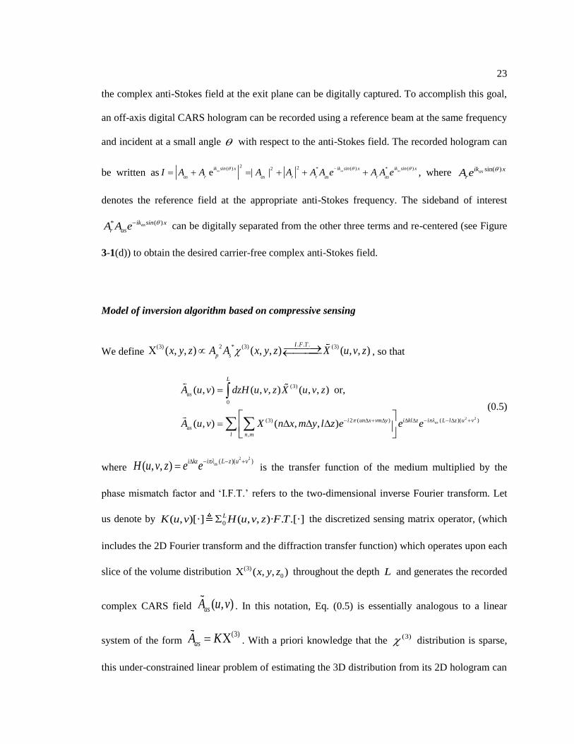
Figure 4-2: Pulse profile of simulated IR and NIR pulses and hypothetical (2) spectrum

used in numerical simulation, (b) simulated SFG spectrogram. 2nd

panel in (b) plots

the line trace at zero delay in spectrogram, which illustrates the loss of resolution

typically inherent in BB-SFG-VS. ................................................................................... 52

Figure 4-3: Simulation of high resolution SFG spectroscopy using 2D PR. (a) SFG

spectrogram of hypothetical transform limited NIR probe pulse and transform

limited IR pump pulse, (b) Estimate of (2) and comparison with simulated

(2)

(c) Error Estimation of spectrogram and response spectrum and the error between

simulated and estimated spectrogram. ............................................................................. 53

Figure 4-4: (a) Simulated SFG spectrogram using hypothetical (2) and chirped NIR

probe pulse. (b) Numerically computed SFG spectrogram using 2D PR, (c) Estimate

of (2) (black dotted curve) computed using 2D PR, hypothetical

(2) (green

curve) and trace of spectrogram through 0 delay (See dotted white line in (b). Notice

that spectrogram trace does not resolve adjacent peaks at 2915 cm-1

and 2920 cm-1

.

(d) Simulated and computed spectral amplitude and phase of chirped NIR probe. ......... 54

Figure 4-5: Schematic of experimental setup (ssp configuration) ........................................... 57

Figure 4-6: Match between experimentally recorded and computationally retrieved SFG

spectrogram of air/DMSO interface. (a) Recorded BB-SFG SFG spectrogram of the

air/DMSO interface taken in the range of ±6.4 ps delay between the 2 ps probe pulse

and broadband pump pulse at ~3.4 μm. (b) Numerically estimated BB SFG

spectrogram using 2D PR. (c) Trace of spectrograms when both pump and probe

overlap with no delay. (d) Trace of both spectrograms along peak of the spectrum. ...... 58

Figure 4-7: (a) RMS error between measured and computed spectrograms. (b) Estimated (2) spectrum of air/DMSO interface ............................................................................. 60

Figure 4-8: Schematic depicting change in fs pulse due to its interaction within a

hypothetical process. Ultrafast pulse characterization can accurately measure

amplitude and phase of fs pulse. ...................................................................................... 61

Figure 4-9: Numerical simulation. (a) Schematic of simulated experiment. (b) Typical

simulated HcFROG trace. (c) 2D F.T. of HcFROG traces at locations ‘P1’ and ‘P2’.

r is the spatial separation between the two locations and gv is the group velocity

through the hypothetical medium. (d) Relative FROG phasor of the pulse at ‘P2’

with respect to ‘P1’. ......................................................................................................... 67

Figure 4-10: Results of numerical simulation using HCFROG algorithm (a) retrieved and

theoretical complex pulse profile. FWHM is marked for pulse at each location. (b)

computed spatial separation between the 3 locations compared with actual

separation used for simulation. The table lists the actual values of spatial separation

as used in the numerical experiment and retrieved using method described. (c)

ix

comparison of retrieved and theoretical pulse spectrum at each location. FWHM is

marked for the pulse spectrum. (d) comparison of retrieved and theoretical SH

spectrum of pulse at each location. FWHM is marked for the pulse spectrum. ............... 70

Figure 4-11: (a) Schematic of our experimental setup. (b) The inset shows SEM image of

the BaTiO3 micro-cluster used for generating FROG signal. (c) Typical recorded

HcFROG trace. The fringe structure can be seen along both delay and wavelength

dimension. ........................................................................................................................ 73

Figure 4-12: Pulse characterization at multiple locations using FROG holography. (a)

Retrieved pulse profile (amplitude and phase, FWHM ~89 fs) at each position; (b)

Comparison of both fundamental and SH power spectrum of the retrieved pulse at

each position with measured power spectra (black squares) (FWHM ~12 nm) (c)

Comparison between retrieved and experimentally recorded spatial separation

between each location with respect to pivot. The table in inset lists actual values in

m . ................................................................................................................................ 74

Figure A-1: Schematic illustrating patterning of PCF for selective filling .............................. 82

Figure A-2 Pumping molten alloy through patterned PCF. (a) Schematic of oven showing

a PCF held in a chamber. The inset shows cutaway of the chamber in which

patterned pcf is held using PDMS and sunk in bath of alloy. (b) Filled PCF under

500 psi showing alloy leaking out as shiny blob from the other end held outside the

oven at room temperature. (c) SEM image of a pcf with three holes filled with alloy,

(d) Setup for checking electrical continuity and typical resistance of filled electrode

(1657 ohms). .................................................................................................................... 85

Figure A-3: Laser welding process for CNT attachment. (a) Side view image of CNT just

prior to being laser welded to alloy filled pcf. Inset shows the schematic top view

illustrating the fiber taper used for delivery. (b) Laser welded CNT. .............................. 87

Figure A-4: FIB assisted CNT attachment. (a) CNT lying on lacie carbon mesh is bonded

to 500 µm tungsten probe tip via Pt deposition. (b) CNT liftoff. Part of carbon mesh

can be seen adhered to the CNT. Individual synapses need to be milled for ‘clean’

liftoff. (c) Sequential targeted attachment of CNT via e-beam assisted tungsten

deposition. (d) Ion beam image of a three-arm device. .................................................... 88

Figure A-5: (a) The average refractive index and extinction coefficients of Ostalloy 158

obtained via ellipsometry of the inset sample, (b) simulation of the typical optical

mode field for the unfilled PCF, (c) the mode field when three of the most center air

holes are filled with Ostalloy ........................................................................................... 89

Figure A-6: Group velocity dispersion for nano-probe with 3 filled electrodes. (a) Mach-

Zehnder setup for spectral holographic measurement. (b) Typical recorded spectral

hologram (c) Measured relative phase, and 3rd

order polynomial fit, (d) estimated

dispersion parameter for unfilled pcf (red dotted) and fabricated device (blue

dotted). Corresponding COMSOL simulated dispersion for unfilled pcf (blue red

line) and modeled device (solid blue line) are also plotted for comparison. The black

curve is dispersion parameter for bare fiber as specified by manufacturer. ..................... 92

x

Figure A-7: Electro-mechanical deflection of fabricated nano-probe. (a) Montage of 3

sequential frames from a video recording CNT deflection. The dotted line shows the

trace along which intensity is plotted in (b) and (c). The markers in (c) indicate pixel

positions of the ‘tip’ of the lower CNT in each frame. .................................................... 94

Figure A-8: Numerical simulation results. (a) charge distribution at the tip of a CNT

when a -20V ramp wave is applied to the terminal, (b) charge distribution along two

CNTs with ±20V applied. The deflection of the CNT is indicated by the red line

which marks the original position, (c) the tip displacement as a function of voltage

applied to the electrodes within the PCF. ......................................................................... 96

xi

LIST OF TABLES

Table 3-1: Coherent Spectrum Estimation: Comparision between theoretical and

numerical results of TwIST applied to Eq. (0.10) ............................................................ 41

Table 3-2: Incoherent Spectrum Estimation: Comparison between theoretical and

numerical results of TwIST applied to Eq. (0.11) ............................................................ 42

xii

ACKNOWLEDGEMENT

I take this opportunity to express my heartfelt gratitude to my advisor Prof. Zhiwen Liu

for guiding me during the course of my PhD program. Prof. Liu is a teacher par excellence and

has the rare ability to provide insight into the subject matter by drawing parallels between

concepts in different fields. I acknowledge his academic mentorship and his lasting influence on

my approach to assimilate new material and creativity towards problem solving.

My workspace was adjacent to Prof. Gopalan who was on my PhD committee and I thank

him for several insightful academic discussions, and especially for showing faith and confidence

in my ability to teach. Prof. Kane and Prof. Khoo equipped me with the knowledge of inversion

techniques and laser fundamentals that was necessary for my PhD projects and I thank them for

their support and encouragement during my search of career opportunities.

I recall joining the lab of Prof. Liu with no experience in an optics lab. Therefore, my

creativity and hands-on skills of working in lab are testament to the crucial support and

contribution of all my labmates. Kebin, Heifeng and Qian showed by example what it takes to

convert a good PhD thesis into a better PhD thesis. Perry set the bar on dexterity in the lab and I

enjoyed many engaging discussions with him, even on topics outside of optics. Chuang and Ding

showed me how not to make common mistakes in lab by actually doing them and always had

joke at hand to fix all problems! I also had the pleasure of working with Corey Janisch, Chenji

Zhang, Yizhu Chen, Alexander Cocking, Atriya Ghosh and Rong Tang and mentoring them when

needed. I have learned that it is because of my labmates that everything works and we all know

why!

I would like to thank my collaborators Christopher Lee and Prof. Seong Kim from Penn

State, and Prof. Yong Xu from Vriginia Tech, with whom I have enjoyed working towards

fruitful research. It is important to also highlight the key contribution of MRI staff, namely

xiii

Trevor Clark and Joshua Maier for their unerring support and patience when I was learning to use

FIB and of Maria and Julie for support when I was the lab manager. I am particularly thankful to

the administrative staff at EE department including SherryDawn Jackson and MaryAnn

Henderson among others for always having my back regardless of whether I had a missing

signature or deadline.

The time of my life that I spent in Happy Valley with my friends in ‘709’ and ‘241D’ is

an integral part of me. I have very fond and special memories with each and every one on them.

Kadappan and Vishesh for being there always no matter what; Himanshu and Aditya for showing

how everything can be fun; Kishen and Ashish for the delightful discussions over tea; Vivek,

Arun, Apoorva, Niddhi, Amruta, Deepti, Nandhini, Piyush, Divya, Adarsh, Aseem, all have

added a unique flavor and I am grateful for their company.

My wife Prachi has always been my best critic. I will remain thankful for her rock steady

support during the uncertain times at later stages of my PhD. It is often difficult to describe the

contribution of your loved ones in the space of few words. I am indebted to my wife, my parents,

and my brother for all their contributions to my success that are best acknowledged with a wink

and for their presence in my life.

1

Chapter 1

Introduction and Motivation

In a general sense, optical sensing is mapping (or encoding) of the optical information of

interest in either time, frequency, space or angular spectrum, or some parameter space specified

by a combination of these domains. A conventional optical image such as a photograph produced

by an imaging lens of a camera is an isomorphic measurement of the light scattering from the

elements in the field of view. Similarly a conventional dispersive spectrometer isomorphically

detects the optical spectrum of the incident light. Optical sensing in general can be modeled as the

detection of the signal of interest f mapped to a set of measurements ( ) ( )i im K q f q dq

where ( )iK q is the sensing system model (which may be isomorphic or anisomorphic, that is an

indirect measurement which needs to be processed to retrieve the signal) and q is a (possibly

multi-dimensional) quantity which parameterizes the basis space, such as time or frequency.

Research in computational optical sensing based on modeling and manipulation of light has

resulted in advances in the overall capability of optical sensing systems by reducing noise,

improving resolution, enhancing measurement sensitivity and dynamic range, enabling higher

dimensional imaging using lower dimensional measurement and allowing for image compression.

For instance, stochastic optical reconstruction microscopy or photo-activated localization

microscopy [1]–[3] achieves significantly higher resolution than the Abbe diffraction limit by

computationally post-processing multiple low resolution images taken using conventional

fluorescence microscope. The field of astronomical imaging can be credited with the invention of

several innovative techniques such as aperture synthesis [4] which enabled high resolution

imaging by electronically correlating signals from individual receivers to synthesize apertures so

2

large that they would be impossible to construct in practice; and wavefront sensing [5] which

advanced earth based imaging by allowing to correct for atmospheric turbulence adaptively

among other applications. Spectral imaging which recognizes the rich information content of the

electromagnetic spectrum combines 2D imaging and spectroscopy and has important application

such as remote sensing and object identification. The data intensive spectral imaging

measurement, which seeks to capture the optical spectrum at every spatial location in image,

benefits from signal acquisition and computational processing techniques, such as tomographic

spectral imager [6] and coded aperture snapshot spectral imager [7], which can retrieve the 3D

image of interest from a lower dimensional simplified measurement. In 1948 Gabor proposed

holography [8], a novel imaging modality which is capable of recording and reconstructing a 3D

representation of an object by detecting the complex optical field originating from the object

instead of only the image intensity, and laid the foundation of optical holography. In fact digital

holography, pioneered by Goodman [9] which involves the use of a digital recording medium and

allows for numerical reconstruction of the object was an early demonstration of the use of

computational techniques for image formation. These examples serve to illustrate that

measurement schemes which involve innovation both in acquisition and signal-processing can

improve existing imaging modalities and potentially overcome limitations imposed by

conventional hardware. Indeed one may observe that the invention of laser and advances in

detector technology such as charge-coupled device (CCD) technology and the complementary

metal oxide semiconductor (CMOS) technology has revolutionized the field of optics by

providing both versatile optics sources and powerful electronic detectors for storage and access.

In this context one can say that the continuous accelerated advances and increasingly cheaper

access to computing resources for optical sensing is similarly having a transformational impact in

optics by enabling modeling of the optics between (and including) the source and detector and the

optical phenomena itself. With the increasing availability of computational resources it has now

3

become possible to abstract physical hardware by developing novel computational techniques

which not only model their functionality but also overcome their limitations. Moreover, access to

computational resources has driven the application of this research outside the laboratory, as

evidenced by familiar medical imaging innovation such as “computer aided tomography”.

Therefore there is clear motivation to explore novel measurement schemes and augment existing

optical sensing methods by leveraging computational techniques developed in other fields of

study. The presented work reflects this trend by focusing on several emerging areas of imaging,

including coherent anti-Stokes Raman holography, high-resolution non-linear spectroscopy, and

spatio-temporal imaging of ultrashort pulse.

Organization

This dissertation presents projects involving application of computational methods and

development of prototype optical measurement systems for overcoming exiting limitations in

several non-linear and ultrafast optical imaging and spectroscopy techniques.

In particular, chapter 2 introduces the computational techniques of compressive sensing

and two-dimensional phase retrieval. Compressive sensing is a novel signal processing paradigm

which seeks to minimize the number of measurements and reconstruct the signal by leveraging

sparsity inherent in the signal. 2D phase retrieval is an iterative algorithm used for obtaining the

phase of a complex-valued field from some intensity measurement involving the field. Both

computational techniques seek to improve key signal metrics such as higher signal to noise ratio

(SNR) and better resolution than can be obtained directly.

In chapter 3, we discuss the application of compressive sensing to imaging and

spectroscopy. In particular, we develop compressive coherent anti-Stokes Raman holographic

imaging to enhance the apparent optical sectioning capability of coherent Raman holography by

4

minimizing out-of-focus background noise. We propose compressive frequency comb

spectroscopy as a novel technique for ultra-high resolution multi-heterodyne optical spectroscopy

and demonstrate its potential over broad spectral range using numerical simulations to study

acquisition of sparse line spectra.

Chapter 4 concerns with the application of 2D phase retrieval to optical imaging and

spectroscopy. We present original demonstration of 2D phase retrieval based technique for high-

resolution sum frequency generation vibrational spectroscopy (SFG-VS) by retrieving the

vibrational spectrum of molecules with significantly improved resolution than can be achieved in

conventional experimental setup. Lastly, as another application of 2D phase retrieval, we

demonstrate coupled spatio-temporal characterization (imaging) of ultrafast optical pulse using

‘holographic frequency resolved optical gating’ (HCFROG) in which the spectral hologram of the

conventional FROG trace is used to map the pulse in space-time with micrometer spatial and

femtosecond temporal resolution.

Finally chapter 5 summarizes the work presented in this thesis and postulates future work

in further leveraging computational techniques towards even more exciting optical imaging and

sensing technologies.

5

Chapter 2

Computational Methods in Optics

Introduction

In this chapter we will review the concept, theory and the application of two

computational methods, namely ‘compressive sensing’ (CS) and ‘two dimensional (2D) phase

retrieval’ in optical data analysis. Essentially both CS and 2D phase retrieval are inversion

techniques in which the signal of interest is retrieved from measurements based on a model of the

signal generation and acquisition system. CS is a theoretical framework in signal processing

paradigm and outlines an optimum sampling strategy by specifying the conditions under which a

signal of interest may be acquired such as to significantly minimize the number of measurements

required for its reconstruction. Phase retrieval is a sub-class of a general class of problems in

which only part of the information in the signal can be measured experimentally and yet the

missing information can be estimated from this partial knowledge by imposing the experimental

and physical constraints in a self-consistent manner using a suitable computational algorithm. In

particular, in phase retrieval an estimate of the missing phase of the object field can be obtained

from a measurement of its magnitude only. Thus arguably both CS and phase retrieval seek to

estimate a signal from an incomplete measurement set that is often times an anisomorphic

representation of the signal of interest.

6

Compressive Sensing

Motivation

It is well known that the Nyquist-Shannon sampling theorem [10] prescribes that any

bandlimited signal can be reconstructed accurately if it is sampled at a rate at least twice as fast as

its largest frequency. By sampling at the data rate, the sampling theorem ensures that information

is not obscured or lost via aliasing which is an artifact of under-sampling. However, it is

commonly observed in practice that signals retain the information content even if they are under-

sampled. For example, the image recorded by a conventional digital camera of a typical outdoor

scene is sampled at the native pixel pitch of the detector and can be huge in terms of data

captured. However, image compression algorithms (e.g. JPEG, PNG, etc.) are practically always

used to reduce the size of digital images for subsequent storage, processing and transmission

despite being potentially lossy because they can retain the essential information using

significantly less data. This suggests that signals of interest can be sampled at the ‘information

rate’ rather than ‘data rate’, or in other words that the signal can be specified using fewer degrees

of freedom than implied by its bandwidth, as in the Nyquist sampling strategy. [11] The question

of efficient sampling of signals such that their reconstruction is accurate is especially important in

optical imaging and spectroscopy. For example, in the field of medical imaging and astronomical

imaging, images are often studied to identify interesting edge-like, point-like or similar localized

features scattered throughout the scene. Clearly the Nyquist sampling criteria is inefficient (and

even prohibitively costly) in such cases since such high contrast features always have very large

spatial bandwidth. Similarly the problem of recording 3D imagery (such as hyperspectral

imagery) can be highly data intensive and experimentally challenging because detectors

inherently capture only 2D data. Even in optical spectroscopy, the ideal requirements of wide

7

scanning range, very fine spectral resolution, high SNR and minimum acquisition time pose

competing challenges to the design parameters of the device.

Description and Formulation

Compressive sensing is the flagship mathematical framework which definitively answers

the question of whether sampling and reconstruction strategies superior to conventional wisdom

exist. The central idea of compressive sensing is to exploit the sparse structure inherent in typical

signal of interest to design efficient sensing and compressing strategy such that an accurate, and

possibly exact recovery of signal is possible. CS leverages two basic principles: sparsity and

incoherence. Sparsity embodies the feature of compressibility of a signal and expresses the fact a

signal may be specified by its ‘information rate’ which can have much fewer degrees of freedom

than implied by its Fourier transform. [11] In other words, it is possible to find concise

representation i.e. a sparse transformation of the signal in which the signal can be expressed in

terms of only few non-zero (or significant) coefficients. Incoherence is the characteristic of a

measurement (encoding) system which allows efficient representation of the sparse signal in the

sense that the information embedded in the sparse signal can be condensed into few

measurements. Formally, we can express the acquisition process in terms of the linear model

y f where y is the set of measurements of signal f and is the system model. Let

denotes a sparse transformation of f into x : f x such that x has only S significant

components (we say x is S sparse) and suppose that a coherence measure can be defined as

1 ,( , ) ( )·max | , |jk

k j nn

. Then low coherence refers to the fact that the sensing matrix

is not correlated with the signal representation matrix . As a familiar example, the model of

conventional Nyquist-rate sampling is a special case of CS in which the Fourier basis, i.e. the set

8

of complex exponential harmonics, which is used for sensing the signal is clearly uncorrelated

with the delta comb which is used to sample the signal (say in time or space). Thus it may be said

that incoherence embodies a more general form of the ‘time-frequency’ duality. [11] This insight

helps in understanding the particularly counter-intuitive aspect of CS which is that it prescribes

the use of random matrices, i.e. matrices which are entirely non-adaptive to the structure of the

signal to guarantee accurate reconstruction of the sparse signal from the significantly incomplete

measurement set. In fact, random matrices with independent identically distributed samples of a

Gaussian or Bernoulli ( binary values) random variable are known to exhibit very low

coherence with any sparsifying basis [12]. Given a low coherence pair of system matrix and

sparsifying basis , the problem of reconstructing x from the measurements y is stated as

0ˆ such that arg min || ||

x

xx x xy f A in which the zero norm

0|| #{ | }|| 0ii xx is simply the total number of non-zero elements in x and A is the overall

sensing matrix. However, it is well known that the 0 search problem is 1 mathematically and

computationally intractable, or ‘NP-hard’. [13], [14] Instead, researchers Daubechies et al., and

Candes, Tao, Romberg and Donoho [15]–[18] proposed a computationally simpler convex

constrained optimization problem of minimization, namely:

1ˆ such that arg min | (P1)| ||

x

x yx Ax

where 1 | ||| || xx to leverage the rich literature available on solving (P1). [19] In particular, it

has been established that the solution x is optimal in the sense that exact recovery is provable for

exactly sparse signals, if the number of measurements is at least

2( , )· ·logM c S N (0.1)

9

where N is the length of the sparse signal x . [17], [18] The best estimate of the original signal f

can then be easily constructed from the sparse coefficients of x using ˆ ˆf x . The condition on

minimum measurements M stated in terms of the coherence measure is effectively a property

required by the system matrix and hence A to enable stable reconstruction. It is well known

that the existence of the null space of under-constrained system matrix A , as is the case in CS

(M<N), allows infinitely many solutions to the linear problem y Ax , i.e. the solution is ill-

posed in general. However the apriori knowledge of sparsity (only S non-zero elements) in x

intuitively suggests that M NS measurements should allow us to overcome this inherent

ambiguity, if the sub-matrix A composed of the columns of A indexed by the support of the S

non-zero elements of x preserves the sparsity. This leads us to define ‘restricted isometry

property’ (RIP) of the system matrix. [17] It states that a matrix A satisfies RIP of order S if

there exists a small constant (0,1) such that for any S-sparse vector x

2

2

1|| ||

1|| ||

A x

x

(0.2)

In other words, RIP as defined in Eq. (0.2) requires that every sub-matrix A formed by choosing

any set of S columns of A be an approximately orthonormal matrix (preserves the length and

structure) of corresponding S-sparse vectors). Since CS assumes no prior knowledge other than

sparsity of the signal, any matrix which satisfies the RIP property describes a linear and non-

adaptive measurement of the signal and can be used for inversion. We now present a brief

discussion of the particular reconstruction technique we have used for our CS–based applications

presented in this dissertation.

10

Reconstruction using TwIST

We noted earlier that the CS based acquisition using the formulation based on

constrained 1 minimization (P1) simplifies a computationally difficult problem by making it

into a convex optimization problem. An important variant of (P1) is the combined 1 2

unconstrained optimization problem [20]

2

2 1

1ˆ || || || || (P2)

2arg min ( ) arg min

x x

x y Ax xh x

which is useful to account for noise in real world measurements via the 2 norm of the error. The

form (P2) is similar to the well-known regularized least squares except that here the convex

objective function h is penalized by the 1 norm regularizer whose penalty is controlled by the

regularization parameter . It is easy to illustrate the fact that the 1 norm penalty promotes the

search for the sparsest solution, which is the aim in CS based reconstruction. Figure 2-1 plots the

values of the 1 and 2 terms in (P2) for a general vector x as a function of the value of an

element ix in that vector. As ix increases, the value of the 2 term 2

2||·|| grows quadratically

whereas the value of the corresponding 1 norm 1||·|| grows linearly.

11

Figure 2-1: Illustration of why 1 norm promotes sparsity. 1 norm regularizer results in higher

penalty for smaller components of signal than its larger components.

This dependence of the 1 and 2 norm implies that the small component in signal are penalized

more than its large components by the 1 norm. In other words, the 1 regularizer favors

significant components in the signal and thus promotes sparsity in CS based signal reconstruction.

In fact, (P2) describes the general form of many problems which arise in signal processing in a

variety of applications such as signal denoising, deblurring, interpolation and compression [20]

apart from compressed sensing. As such, huge body of literature has been developed prior to the

discovery of CS theory to computationally solve the problems of the form (P2), notable amongst

which are the basis pursuit [17], [18], [21] and LASSO [22] techniques. One of the approaches is

the iterative shrinkage thresholding (IST) family of algorithms. Donoho et al. [23] pointed out

early on the connection between shrinkage and 1 norm penalty in context of superresolution of

nearly sparse astronomical image recovery. Donoho and Johnstone also demonstrated the idea of

‘thresholding’ as a suitable technique for reconstructing signals from noisy measurements in the

context of wavelet based image deconvolution. [24], [25] In recent years many researchers have

studied different aspects of iterative shrinkage thresholding algorithms. In essence, the IST

12

algorithm operates independently on each component of the sparse vector x by either shrinking

it or setting it zero, based on its value compared to the preset regularization parameter . In fact,

this shrinkage/thresholding operator perturbs the solution obtained by the standard gradient

descent method in every iteration. This nonlinear shrinkage thresholding operator )·( is given

by,

1 1(1 ) ( ) ( ( ))

( [ ]) ( [ ]) max{0, [ ] }; [ ]

( [ ]) max{0, }; [ ]

·

T

n n n n n

i i

x x x x A y Ax

x n sign x n x n x n

x n e r x n re

(0.3)

The flavor of IST that we have implemented in this work is a two-step algorithm called ‘TwIST’,

which gets its ‘two-step’ description from the fact that the next iteration 1nx depends on

previous two iterations nx and 1nx , as can be seen from first sub-equation in Eq. (0.3). [26] (We

refer the interested reader to Ref. [26] for the definition of parameters and and for

additional details.) In this dissertation, we use TwIST algorithm to demonstrate application of CS

for optical imaging and spectroscopy. In particular, we demonstrate significant reduction in noise

and hence apparently enhanced optical sectioning capability of coherent Raman holographic

imaging modality, and propose a novel compressive optical spectroscopy scheme based on the

use of frequency combs

13

Two Dimensional Phase Retrieval

Motivation

The problem of 2D phase retrieval belongs to the general class of problems encountered

in several areas of optics, namely the determination of a complex function from a limited

knowledge of its Fourier transform. Mathematically, if we consider an object ( )f q and its

Fourier transform ( )( ) ( ) iF R e u

u u which are related via the standard definition:

( ) ( )ex ·21

2p( )F f i d

u qu q q and ( ) ( )ex

1·p( 2 )

2f F i d

u qq u u , then we are

interested in the solution to the problem of obtaining the phase ( ) u from a measurement of

2| ( ) |R u subject to constraints on ( )f q based on its specific characteristics. Here q (and

hence u ) is a vector whose elements specify the multi-dimensional basis for the support of the

object. Thus in the typical phase retrieval problem in optics, the goal is to obtain the phase of a

complex object from a measurement of the squared modulus of its Fourier transform. Phase

retrieval problems are commonly found in several areas in optics. For example in x-ray

crystallography, information of the electron density function characterizing the crystal structure is

contained in both the amplitude and phase of the observed diffraction pattern, however only the

intensity of the diffraction pattern can be measured experimentally. The technique of wavefront

sensing for compensating optical aberrations in an imaging system relies on obtaining an estimate

of the complex optical transfer function from its measured point spread function which is related

via the Fourier transform. Indeed such a technique was successfully applied to design the

compensating optics of the famous Hubble Space Telescope [27], [28] and resulted in spectacular

improvement of its imaging capability. In these and several other problems in optics, the

measured signal is related to the magnitude of Fourier transform representation of the signal of

14

interest. The importance of the problem of phase retrieval lies in the fact that in general the

magnitude of Fourier transform of the signal alone is not sufficient to uniquely specify the

complex signal. For example if the unknown signal is filtered with an all-pass filter then the

measured signal has the same spectral amplitude but different spectral phase so that signal

recovery may become impossible in the absence of additional constraints on the measurement

model or signal itself. The importance of the knowledge of phase for complete determination of

the signal has been demonstrated by the work of Srinivasan [29], Oppenheim [30], and other

investigators. In fact these researchers have shown that a signal synthesized by using only its true

phase function in combination with some amplitude function (even if the amplitude function is

unrelated) can bear close resemblance to the actual signal.

Uniqueness

It is well known that the one dimensional (1D) phase retrieval problem has no unique

solution and it is in fact plagued by the existence of many nontrivial solutions [31]. On the

contrary, solution of the 2D phase retrieval problem in which the support of ( )f q is two

dimensional, for example the x and y coordinates of an image, is overwhelmingly likely to be

unique in practice aside from the trivial ambiguities of mirror image (i.e. inversion in origin) and

a constant shift. The important question of uniqueness of the 1D and 2D phase retrieval has been

investigated by several researchers; see for example [32], [33], [34]. The key argument which

explains the uniqueness criteria of the solution of the general phase retrieval problem hinges on

reducibility (or ‘factorability’) of a polynomial in one or more dimensions. While the complete

mathematical arguments discussing uniqueness are beyond the scope of this dissertation, we

intend to present only a distilled and simplified discussion to highlight how the ability to factorize

polynomials results in very different non-unique solutions to the 1D phase retrieval problem, but

15

enables practically unique solution to the 2D problem. The analytic continuation of the Fourier

transform of the signal of interest via the change of variable 'i u u u z is given by

( ) ( )ex ·21

2p( )F f i d

q zz q q . Under the assumption that ( )f q has finite support and is

of finite energy, it is known that ( )F z can be expressed as the Hadamard product

1(1 /( ) )kF

kz zz [35] where kz are complex zeros of the analytic continuation. This

implies that any 1D signal can be specified uniquely by the set of the complex zeros of its

analytic continuation in the complex plane. In many optics experiments the squared modulus of

the Fourier transform 2( ) | ( ) |I Fu u is the measurable and relates to the autocorrelation of the

signal via the Parseval’s theorem. The analytic continuation of ( )I u is given by

1( )() )( kI

*

k kz z z zz so that ( )I z is characterized not only by kz but also by the

set of complex conjugate zeros *

kz which are the zeros of * *( )F z . Now it can be shown that the

so-called ‘Blaschke factor’ ( ) / ( ) k

*

kz z z z allows synthesis of a different function

1( ) ( )[( ) / ( )]F F *

kkz z z z z z which has the same squared modulus 1( ) ( )I Iu u but which

is specified by *

kz , i.e. zeros that are ‘flipped’ across the real axis. In other words, only the

knowledge of the intensity measurement ( )I u does not allow unique determination of the

complex functions ( )F z or 1( )F z . Thus the reducibility of a 1D polynomial into N complex

zeros results in 12N

-fold ambiguity (not counting the trivial ambiguity resulting from flipping

all zeros that forms the set of mirror image functions) of whether the zero or its complex

conjugate informs the observable quantity ( )I u . This mathematical argument in Fourier domain

has a very familiar manifestation in the signal domain. We note that it is common knowledge that

two signals with significantly different distribution can have visually indistinguishable

16

autocorrelation shapes. [36] However, the story changes completely in the case of functions of

more than one variable. In fact, the fundamental theorem of algebra does not guarantee such

reducibility for nearly all polynomials of interest in two variables, which is the situation in the 2D

phase retrieval problem. Therefore the polynomial reducibility argument presented above does

not hold for the 2D case. This mathematical fact essentially allows the existence of unique

solutions for the 2D phase retrieval problem in practice, (except the trivial ones of inversion in

origin and constant shift noted above), and motivates investigation into techniques for finding the

unique solution.

Solution using Generalized Gerchberg-Saxton Algorithm

One early technique for phase retrieval proposed initially by Wolf [37] and developed

later by Mehta [38] involved use of exponential filters to effectively measure the modulus of

analytic continuation of its transform and use mathematical techniques to reconstruct its phase

from this measurement. Other techniques demonstrated include an interferometric measurement

of the correlation function with known reference field [39]–[41], a maximum-likelihood estimator

for the phase constrained by the measured modulus [42]–[44] and a host of analytical and

experimental techniques which are based on applying the constraints imposed by the analytic

properties of the correlation functions [see list in Ref 4 of [45]]. A notable numerical technique

was the Gerchberg-Saxton iterative algorithm (GS) [46], [47] for estimating phase from two

intensity constraints in the object and its Fourier domain. By far the most successful and

commonly used technique for solving for the estimate of the 2D phase retrieval problem is the

error reduction algorithm due to Fineup [48] who demonstrated “dramatic” efficacy of retrieved

objects by modifying and generalizing the constraints of the GS algorithm.

17

Figure 2-2: Generalized Gerchberg-Saxton algorithm: error reduction algorithm

It is depicted pictorially in Figure 2-2, where we have used two variables explicitly to emphasize

the 2D phase retrieval problem in particular. As can be seen, the generalized GS algorithm is used

to solve the 2D phase retrieval problem by iteratively transforming between the object and

Fourier domains while applying the constraints in each domain dependent on the model of

generation of object field (i.e. signal of interest) until the solution converges as determined by a

particular error metric. The error reduction algorithm by Fineup has been treated by the method of

generalized projections by Levi and Stark [49], [33]. In this approach, each constraint applied in

the object and the Fourier domain defines a set of permissible functions, and imposing the

constraint is equivalent to finding the projection of the solution on that set. In this sense, the error

reduction algorithm operates by projecting the current estimate on each constraint set sequentially

and iteratively to seek a point in that set closest to the estimate such that a certain error metric is

minimized. The generalized projection implementation is depicted pictorially in Figure 2-3 which

also shows the ‘seed’ for the iterative algorithm. The arrows depict the progression of iterative

algorithm and convergence is indicated by the fact that the solution moves progressively ‘closer’

to both constraint sets simultaneously.

18

Figure 2-3: Generalized projection method description of GS based error reduction algorithm

Thus solving the phase retrieval problem using the generalized projections method is akin

to finding a member of the intersection of all constraint sets. The method of generalized

projections allows at least one of the sets to be non-convex, as indicated in Figure 2-3

which is true in case of phase retrieval since the measured Fourier modulus imposes a

non-linear constraint. Convergence is reached when the point being sought lies in the

intersection of both constraint sets and the overall error is lowest.

In this dissertation, we will show that the problem of spatio-temporal

characterization of ultrafast laser pulse and the problem of high resolution of nonlinear

spectroscopy can be stated as 2D phase retrieval problems. Our solutions obtained by

applying the error reduction algorithm demonstrate enhancements to overcome

limitations with existing techniques in both optical imaging and spectroscopy in line with

the theme of this work.

19

Chapter 3

Applications of Compressive Sensing

Introduction

We overviewed the concept, theory and reconstruction techniques of compressive sensing

in chapter 2. It was seen that CS is a novel approach in signal processing at ‘information-rate’

with the key advantage of minimizing the number of measurements by leveraging sparsity

inherent in typical signals of interest. In this chapter we will demonstrate the impact of this

distinguishing advantage of CS in optical imaging and spectroscopy by considering two important

applications: label-free, non-scanning 3D microscopy, and very high resolution frequency comb

spectroscopy. We will lay out the importance of both applications, motivate enhancements to

overcome existing limitations and formulate the optical problem in the appropriate framework to

demonstrate the enhancements using CS based signal recovery.

Compressive off-axis coherent anti-Stokes Raman scattering holography

Introduction

Optical microscopy based on fluorescence imaging is highly mature and standard

imaging modality for observing biological samples and is an indispensable tool in a typical

scientific laboratory. It is well-known that fluorescence microscopy requires staining the sample

using specific fluorophores to enable discrimination between different chemical species in the

sample. This sample preparation step has the adverse effects of photo-bleaching in which the

fluorophores lose their ability to fluoresce, severely limiting the exposure time, and photo-

20

toxicity, hindering the long-term imaging of live specimens. Additionally traditional focal-plane

imaging techniques (such as conventional fluorescence microscopy) have poor axial resolution

due to the lack of optical sectioning and generally their image quality suffers from a relatively

strong unfocused background. Confocal microscopy [50]–[52] successfully eliminates out of

focus fluorescence signal and significantly improves axial resolution to enable 3D imaging. Two-

photon fluorescence is another novel imaging technique which not only suppresses the

background (due to it being a non-linear process) but also penetrates deeper and minimizes

scattering in the sample. However in these techniques the resulting 3D image is acquired by

scanning the sample in all three spatial dimensions or scanning the excitation beam. The principle

of holographic imaging invented by Gabor [8] allows single-shot multi-focal plane imaging

without the need for axial scanning. Holography is capable of 3D reconstruction of the source by

recording the amplitude and phase of the complex optical field and hence measuring its (limited)

angular spectrum. With the inception of digital holography [9], the ability to digitally record the

optical field has enabled digital algorithms based holographic reconstruction using the diffraction

theory (i.e., digital focusing). This suggests that if a suitable imaging technique which can

discriminate chemical species without staining biological samples were to exist, its combination

with holography can potentially enable a powerful and live 3D imaging capability. In fact, Raman

scattering is indeed such a phenomena whose optical spectrum is characteristic of the intrinsic

vibrational response of the molecular species. The Raman response of a molecule therefore

provides a characteristic vibrational spectral ‘fingerprint’ for detection. This spectral ‘fingerprint’

can be exploited as a chemically selective ‘label free’ contrast mechanism. In contrast to

spontaneous Raman emission, coherent Raman scattering features orders of magnitude improved

sensitivity since the molecular response is driven coherently by tuning a pair of coherent

excitation sources to excite the vibrational mode(s). In this work, we restrict our attention to

coherent anti-Stokes Raman scattering (CARS) to integrate with holography. CARS was

21

originally observed by Maker and Terhune as coherent, directional and blue-shifted radiation

which is free from one-photon induced fluorescence [53]. After the demonstration of scanning

CARS microscopy by Duncan [54], Zumbusch et al. [55] re-ignited the field by demonstration of

their 3D sectioning capable scanning CARS microscope using tightly focused beams. Digital

CARS holography [56]–[59] on the other hand uses holographic imaging principle to capture the

complex anti-Stokes field produced in a sample upon excitation with a pump/probe and a Stokes

beam, and therefore features the desired label-free, chemical selective, and scanning-free, single

shot 3D imaging capability. However traditional digital propagation based reconstruction using

CARS holograms results in images whose quality suffers due to presence of out-of-focus

background. It can be shown that since the angular spectrum of the source distribution is

effectively low-pass filtered (/band-limited) in holographic measurement, the problem of

retrieving the exact source distribution using a single hologram does not permit unique solution

[60]. Numerical inversion techniques using 1 norm as regularizer have been proposed for

holographic reconstruction [61]–[65] to assist in the solution of the under-constrained problem of

estimating 3D distribution from 2D image. In particular, D. Brady et al. [66] has recently

demonstrated that compressive sensing based algorithms can estimate a sparse volumetric sample

distribution from a single two-dimensional hologram thereby reducing the number of

measurements required as compared to diffraction tomography. Compressive holographic

reconstruction has also been applied to inline CARS holography [58]. Here we present

compressive off-axis CARS holography to enable noise-suppressed inference of volumetric

source distribution of (3) from measured complex anti-Stokes field. In particular, using

compressive CARS holography, we show the significant reduction of out-of-focus background

noise while estimating the sparse volumetric distribution from a single CARS hologram.

Complex valued numerical model of the holographic reconstruction method, including the

22

complex valued measurement as in our case, improves the performance of compressive sensing

based inversion algorithms by allowing the system matrix to be well-conditioned.

Formulation

Model of signal generation

The model of compressive CARS holography can be understood as the linearization of the

equation governing the formation of a CARS hologram from a given (3) ( , , )x y z source

distribution. The pump field pik r

p pE A e

and Stokes field sik r

s sE A e

excite molecular

vibrational modes in a sample of thickness L. The probe field is assumed to be the same as the

pump. The resultant anti-Stokes field is given by · ˆ, , asik z

s

z

sa aE A x y z e ( z is the unit vector of

ask ). The amplitude of the anti-Stokes field in the frequency domain is given by [59]:

2 2

( )( ) / ( 22 * (3)

0

)

( , , ) ( , , ) x asy

L

i L z ki kz

as p s

k k

A A du v L A e u v z ez

(0.4),

where the tilde represents the two dimensional Fourier transform with respect to x and y, and

ˆ(2 ·)p s as

kz k k k zz is the phase mismatch. Eq. (0.4) can also be written in the spatial domain,

i.e.,

2 2( )

(3)

0

( )( , , ) ( , , ) / ( )as

L x yi kz

as a

L z

s

i

A x y L x y z i Lze e zd

, where as is the anti-Stokes

wavelength. In other words, the output field is simply the summation of the diffracted anti-Stokes

field generated at each slice in the volume distribution. This observation motivates the application

of digital back-propagation for retrieving the unknown volume source distribution, provided that

23

the complex anti-Stokes field at the exit plane can be digitally captured. To accomplish this goal,

an off-axis digital CARS hologram can be recorded using a reference beam at the same frequency

and incident at a small angle with respect to the anti-Stokes field. The recorded hologram can

be written as2 *

2( ) ( ) ( )*2

e | |a as assik sin ik sin ik sin

as r as

x x x

r asr as rI A A A A A A e A A e

, where sin( )asik

r

xA e

denotes the reference field at the appropriate anti-Stokes frequency. The sideband of interest

( )* asik sin

as

x

rA A e can be digitally separated from the other three terms and re-centered (see Figure

3-1(d)) to obtain the desired carrier-free complex anti-Stokes field.

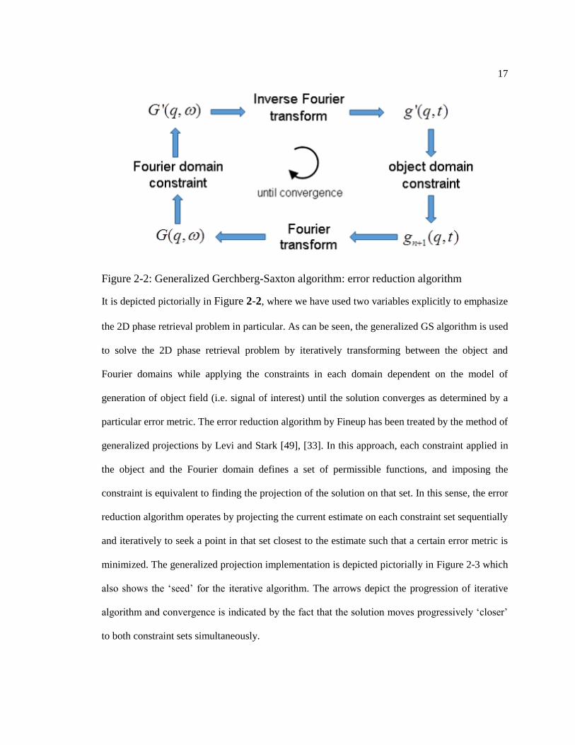
Model of inversion algorithm based on compressive sensing

We define (3) 2 * (3 . . .) (3)

( , ( ,, ( , )) , ) ,p s

I F T

A x y z u v zx y z A X , so that

2 2

(3)

0

(3) ( ) )( )2 (

,

( , , ) or,

, ,

( , ) ( , , )

( , ) ( ) as

L

as

un x vm y i kli L l vz i z u

as

l n m

A dzH u v z X

A X x m y

u v u v z

u v n eel ez

(0.5)

where 2 2

( )( )( , , ) as

i L z u vi kzH u v z e e

is the transfer function of the medium multiplied by the

phase mismatch factor and ‘I.F.T.’ refers to the two-dimensional inverse Fourier transform. Let

us denote by 0( , )[ ] ( , ,· · . ·]) .[LK u v H u v z F T the discretized sensing matrix operator, (which

includes the 2D Fourier transform and the diffraction transfer function) which operates upon each

slice of the volume distribution 0

(3) ( , , )x y z throughout the depth L and generates the recorded

complex CARS field ( , )asA u v . In this notation, Eq. (0.5) is essentially analogous to a linear

system of the form (3)

as KA . With a priori knowledge that the (3) distribution is sparse,

this under-constrained linear problem of estimating the 3D distribution from its 2D hologram can

24

be solved using the method of compressive sensing. In particular, we use the two-step iterative

shrinkage thresholding (TwIST) algorithm [26] to solve for the source 3D distribution by

minimizing the objective function 1

(3) (3) 2 (3)

2( ) 0.5 || || || ||asf A K where is the

regularization parameter. In light of the fact that the measurement is complex valued (because the

hologram records both amplitude and phase), the 1 norm constrained objective function can be

minimized using a complex thresholding operator to iteratively update the next estimate of (3)

using the TwIST algorithm (see remark 2.5 in [15]). The results of the volume distribution

retrieval using the single shot recorded CARS hologram are discussed in the next section.

Numerical Results and Discussion

CARS holograms were recorded using the experimental setup detailed in Ref.[59],

whereby a pulsed nanosecond laser supplying the pump/probe beam and a type II OPO was used

to generate the Stokes and reference beams. The pump/probe and Stokes beam are incident on a

sample consisting of multiple polystyrene spheres which are sandwiched between two glass slides

and immobilized using UV curable glue. When the Stokes wavelength is tuned to match one of

the molecular vibrational frequencies of polystyrene (Raman resonance of polystyrene at 3060

cm-1

) a strong CARS signal can be observed. This anti-Stokes signal was then combined with a

reference beam at the identical wavelength and propagating at a small off-axis relative angle of

approximately 1.7o and the resultant hologram was digitally recorded on a CCD camera as shown

in the schematic in Figure 3-1(a). The recorded hologram of multiple polystyrene microspheres

used in this study is shown in Figure 3-1(b). The two-dimensional Fourier transform shown in

Figure 3-1(c) reveals the expected sidebands for this off-axis recorded hologram, of which we

digitally retain only one sideband Figure 3-1(d). The inverse Fourier transform of the re-centered

25

sideband is the complex anti-Stokes field recorded in the hologram. Figure 3-1(e) shows the

amplitude of the complex diffracted CARS field at the detector plane. It shows the ring-like

features associated with the diffraction of the signal originating from each polystyrene sphere.

The complex field is used as the input for our algorithm to estimate the source 3D distribution.

Figure 3-1: Schematic of CARS holography (a) Schematic diagram of CARS holography (b)

Central part (256x256 pixels) of a recorded CARS hologram; (c) DC filtered two dimensional

Fourier transform (amplitude) of the hologram in (b); (d) A digitally filtered and re-centered

sideband; (e) Reconstructed CARS field (amplitude) at the recording plane.

Figure 3-2 shows typical images of the distribution of the microspheres in a series of ‘z’

slices, ranging from propagation distance of 5 μm to 14 μm, in steps of 1 μm. The out-of-

focus background noise is clearly seen affecting the image quality in each slice. We then

use the TwIST algorithm to iteratively minimize the 1 constrained objective function to

retrieve the image in each slice. The regularization parameter is chosen by trial and

error, i.e., by running the algorithm as varies from 510 to

410. A typical

reconstructed distribution of microspheres in each of the 10 ‘z’ slices is shown in Figure

3-3. We notice that the image in each slice is visually seen to have reduced noise and

sharper images.

26

Figure 3-2: Image reconstruction using conventional digital propagation. The nine polystyrene

microspheres are visible, but the image quality is affected by out-of-focus background

contributions.

Figure 3-3: Compressive sensing based image reconstruction using the TwIST algorithm. The

diffraction noise is suppressed and the spheres signal can clearly be seen to be localized at

different depth positions. Red arrow indicates spheres used for SNR analysis in Fig. 4.

27

To help better appreciate the improvement of image quality and removal of out-of-focus noise, in

Figure 3-4 (a-b) we plot the signal-to-noise ratio (SNR) for two spheres (indicated by arrows in

Figure 3-3) as function of the z depth position. The ‘signal’ is computed as the mean value of a

small 5x5 pixel region around the sphere center, and ‘noise’ is computed as mean value of the

background in the immediate neighborhood of the sphere, within a 101x101 pixel region. The

dotted curves are Gaussian fit to the SNR. It is clearly seen that as compared to the conventional

digital propagation algorithm, our compressive CARS holography technique improves the

localization of the spheres along z, because it minimizes the out-of-focus background noise. This

is further corroborated by Figure 3-4(c-d), which shows an axial slice of the reconstruction of the

lower sphere. The apparent improved “sectioning” occurs because the 1 constrained inversion

favors the strong signal in the image plane and shrinks the weak signal (noise) based on an

empirically chosen threshold constant. Since compressive sensing algorithms search for the

sparsest image, the apparent optical “sectioning” is ultimately limited by the inherent sparsity of

the sample.

Figure 3-4: Axial localization using compressive CARS holography. (a) and (b) show SNR for

two spheres (indicated by red arrows in Fig. 3 along the z depth position using conventional

digital back-propagation algorithm and compressive reconstruction, respectively.

28

Conclusion

We have demonstrated the efficacy of using compressive sensing for 3D label-free

chemically selective volumetric estimation through off-axis compressive CARS holography.

Although off-axis CARS hologram helps remove the twin image noise associated with inline

holograms, the traditional digital propagation based retrieval still suffers from out-of-focus

background noise due to the limited axial resolution, which is inherent in the fact that the

hologram only samples a very small subset in the ‘k-space’ describing the volume distribution of

the sample. It is well known that diffraction tomography can help improve axial resolution

through sampling a larger subset of the object ‘k-space’. If the volumetric distribution of interest

has sparse features, compressive off-axis CARS holography can emulate the higher axial

resolution using only a single shot CARS hologram compared to multiple field measurements

and/or rotation of the sample required for diffraction tomography.

29

Compressive Frequency Comb Spectroscopy

Introduction and Motivation

High resolution optical spectroscopy is a vital tool for research in fundamental science as

well as for enabling technological applications. The pioneering work of Fraunhofer in 1814 and

later Kirchoff and Bunsen in 1859 (among other luminaries) in showing that each atom and

molecule can be identified by its characteristic spectrum established optical spectroscopy as a

preeminent scientific tool for optical interrogation of matter. For centuries, optical spectroscopy

has thus been pivotal in enabling astrophysicists to probe the chemical make-up and evolution of

our vast universe. A state of the art spectrometer featuring resolution of 150 kHz at 500 THz can

facilitate Doppler shift measurements (~ 101/ ~ 0ev c ) to enable detection of candidate Earth-

sized planets [67]. Indeed, a very high resolution spectrometer can make it possible to observe the

expansion of the universe in real-time by tracking the galactic Doppler shifts. In physics, the

capability to measure frequencies with extremely high resolution and Hz-level accuracy allows

for measurement and tracking of slow drifts in fundamental physical constants. For example, the

Hz-level measurement [68] of the 2466.061 Thz 1S-2S transition in atomic hydrogen with a line

width of a 1.3 Hz can allow determining Rydberg constant. The significance of the ability to

precisely measure the Rydberg constant is evident in the fact that it helps define bounds on the

values of other physical constants [69]. The capability to measure optical spectra with high

precision and stability also has important technological applications. For example, identification

of drugs [70] and biological species [71] has implications in medical, health and security industry.

Similarly, molecular fingerprinting of gas molecules [72] and characterization of optical devices

(such as high-Q micro-cavities [73]) can lead to design of optical sensors with unprecedented

sensitivity with applications such as non-invasive sensing of oil and gas.

30

Compressive Frequency Comb Spectroscopy strategy

A desirable spectrometer can be described as having wide spectral coverage, high

resolution throughout its spectral range, fast acquisition, high throughput (large signal-to-noise

(SNR)) and high sensitivity. The operating principle of most conventional optical spectrometers

falls in either of two categories: dispersive or interferometric. Dispersive spectrometers typically

use a grating to disperse incident light and the resolution is dependent on the groove density, size

of grating, and the size of entry and exit slits. Fabry-Perot interferometer can achieve higher

spectral resolution but typically have a limited free spectral range. Fourier transform spectroscopy

(FTIR) is the predominant method of measuring optical spectra in the IR wavelength range whose

operating principle is based on the Wiener-Khinchin theorem. In addition to high throughput,

FTIR spectrometers feature higher resolution and allow multiplex measurement of optical

spectrum, but they employ an optical delay line which requires scanning the reference path. These

conventional spectrometer designs can provide wide coverage over UV, visible and infrared, but

are typically limited to a resolution of about 0.01 nm in the visible (~=10 GHz), which can be

improved if used in conjunction with a virtually imaged phased array [74].

The advent of octave spanning frequency comb using a mode-locked laser [75], [76], [77]

has ushered in a new era of ultra-high resolution optical spectroscopy with orders of magnitude

improved resolution potentially limited only by the Hz-level linewidth of the comb mode. The

principle of an optical frequency comb was described by Hansch et al. in 1977 [78] who showed

that the evenly spaced train of narrow pulses from a stabilized mode-locked laser corresponds to a

comb in the frequency domain. The defining feature of the frequency comb is the highly stable

and strictly periodic arrangement of its modes over a large optical bandwidth thereby providing a

reliable phase-coherent link between the RF and optical domains, not available hitherto. The

frequency comb has been utilized to calibrate astronomical spectrometers beyond state-of-the-art

31

accuracy of 6 MHz (~9m/s Doppler shift) [79]. The frequency comb lends itself naturally to a

massively parallel heterodyne scheme using its modes as the local oscillators (LO).

Optical spectroscopy using the heterodyne technique has been demonstrated [80]–[85] by

mixing a reference frequency comb with a dedicated signal comb which has a slightly different

repetition rate. Continuous frequency coverage may be achieved at the expense of the acquisition

speed by actively manipulating the repetition rate of one of the combs [86], or by scanning the

offset frequency. However we note that optical spectra of interest sometimes consist of only few

characteristic narrowband lines which may be widely separated, for example corresponding to the

energy levels of an inhomogeneous (multi-species) sample. In other words optical spectra are

often ‘sparse’ signals. Efficient measurement of such sparse signals is the focus of large body of

literature in information theory. Recently, compressive sensing is being extensively developed as

general signal processing paradigm for efficient acquisition of sparse signals such as above

mentioned optical spectra, in order to minimize the number of measurements and accurately

reconstruct the signal. By exploiting the unique characteristic of optical frequency comb as a

source of precise and stable optical LO, with the simple yet powerful signal acquisition and

reconstruction strategies based on compressive sensing, here we present ‘compressive multi-

heterodyne optical spectroscopy (CMOS)’ which is a novel technique for ultra-high resolution

optical spectroscopy. We propose multiplexed acquisition of optical spectrum by combining it

with a dynamically encoded frequency comb to map the multi-THz optical band to few GHz-wide

RF baseband. We leverage the sparsity exhibited by optical spectra of interest by compressive

sensing based acquisition strategy [17], [18] to minimize the number of RF measurements

required to reconstruct the optical spectrum with high fidelity. The spectral resolution achievable

by our method is not dependent on the mode spacing of the comb, but rather determined by the

RF instrument used for spectrum measurement. The accuracy of our technique is potentially

32

limited only by the Hz-level uncertainty [87] of the frequency comb, since the accuracy of

heterodyne detection is ultimately determined by the stability of the LO.

Formulation

Our formulation for acquisition of the optical spectrum involves modeling the heterodyne

mixing of the frequency comb and the signal. We begin by analyzing the signal generated in a

photo-detector by combining a real optical signal ( )s t with a real frequency comb ( )c t whose

repetition rate is rf ( 2r rf ). The photo-detector output is proportional to the interference

term in the time averaged intensity ( )· of the incident field

2 2 2 2( ( ) ) ( ( ) ( )) 2 ( ) ( ) ( ) ( ) .e t s t c t s t c t s t c t By using a balanced detection

scheme [88] to retain only the interference term, we can analyze the output m(t) as,

*

* *

0 0

( ) ( )

1( ) ( ) . .

( )

2

n nj t j t

n n

n

j t j t

n n n n

n

s t c e c e

S c e d S c e d c

m t

c

(0.6)

where ( ) F.T.[ ( )]S s t is the Fourier transform of ( )s t and nc is the complex Fourier series

coefficient corresponding to the thn comb mode. It is assumed that the detector is fast enough to

measure only the difference frequencies | | .n Equation (0.6) shows that the spectrum of

the RF signal includes contributions from the ‘image’ pair n as well as .n A

low pass filter (LPF) with a cutoff frequency of / 2LPF rf can be used to define the

spectral coverage of the RF spectrum F.T.[ (( )]) mM t (see Figure 3-5(a)). The different

frequency variables are indicated on the frequency axis shown in Figure 3-5(b). Then the RF

spectrum is

33

* *( ) ( )) ;( n n n n LPF

n

M S c S c (0.7)

By mapping each spectral sub-band 1,( )n n to the same RF window, Eq. (0.7)represents a

particular multiplex measurement ( )M of the entire optical spectrum. Multiple such

measurements may be recorded by dynamically encoding the weight of the comb modes; and the

optical spectrum can be reconstructed by solving the resulting system of linear equations. To do

this, as shown in Figure 3-5(a), the frequency comb can be filtered by using a pulse shaper

consisting of a programmable spatial light modulator (SLM) [89] to digitally control the

reflection or transmission coefficient of each SLM pixel. The encoded comb can then be mixed

with the signal in the balanced detector. The balanced detector removes the d.c. term from the

beat signal and also helps to increase the SNR by common-mode rejection of noise. The RF

interference signal is finally filtered through the LPF and measured by using either a digitizer and

Fourier transform block (D-FFT) (complex amplitude spectrum) or a spectrum analyzer (SA)

(power spectrum).

34

Figure 3-5: (a) Illustrative schematic for CMOS. The frequency comb is first filtered by

weighting its comb modes with a digitally controlled SLM and then combined with the signal

from the sample. The balanced detector measures the RF beat signal between the reference comb

and signal. The RF signal is further filtered by a Low Pass Filter (LPF) and detected by a

spectrum analyzer or a D-FFT block. The broadband quadrature phase-shifter is used to generate

a / 2 phase shifted copy of the comb for the coherent case. (b) Frequency axis indicating

relative value of frequency variables. D is the characteristic response time of the fast detector.

(*diagram is not to scale)

35

Heterodyne measurement of coherent optical signal

The RF spectrum )(M contains contributions from both spectral components

)( nS and )( nS via the thn mode nc . For an ideal coherent optical signal, we can

devise a scheme [90] to resolve the ‘image’ components by additionally mixing it with a / 2

phase-shifted comb, ( ).jc t This scheme may be implemented by sequentially selecting the two

orthogonal linearly polarized components from a circularly polarized comb (prepared by using a

broadband quarter-wave plate, e.g., Fresnel rhomb), and projecting them to the same linear

polarization state by using a 45o-tilted linear polarizer. Figure 3-5 schematically shows the

broadband quadrature phase-shifter to choose between the two copies of the comb. The resulting

model describing the RF spectrum of coherent optical spectrum can be simplified as

*( ) ( ) ;c n n LPF

n

S cM (0.8)

Heterodyne Measurement of incoherent optical signal

In the case of incoherent optical signal, for stationary, ergodic random processes the

spectral density is well defined and can be measured. Mixing of mutually incoherent signals has

been used, for instance, in the determination of laser line-width by measuring the power spectrum

of the beating signal resulted from mixing the laser field with its significantly time-delayed hence

incoherent copy [91]. Note that *( ) ( ) ( ) ( ),S S P where ( )P is the spectral

density of the incoherent signal [see sec 2.4 in [92]]. The model for spectral density of the

measured RF signal is therefore given by:

2( ) | | ( ( ) ( ));P n n n LPF

n

M c P P (0.9)

36

Spectrum Estimation Using Compressive Sensing

Our measurement strategy involves the superposition of a very large number of optical

bands (up to 4~ 10 ) weighted by the encoded comb modes. We noted in chapter 2 that one of the

characteristics of a good system sampling matrix is that it should be maximally incoherent with

the signal representation basis. In our case the signal is the sparse spectrum, so that the signal

representation basis is the identity matrix. Therefore a random matrix appears to be good choice

for the system sampling matrix. We propose to encode the frequency comb with a binary random

matrix consisting of independent identically distributed samples of a Gaussian random variable

which is also known to satisfy the RIP condition [12]. Below we describe how the system model

can be modified to account for the selectively weighted frequency comb (which may be

implemented for example by using a programmable SLM. Then a sparse optical spectrum may be

retrieved from several multiplexed measurements of the form given by Eq. (0.8) or Eq. (0.9).

Coherent spectrum estimation

To represent the dynamically weighted modes of frequency comb as described before, the

coefficient of the mode *

nc should be replaced by *( ) ( ) * ,k k

n n nf w c where ( )k

nw are the

programmable weights during the thk measurement. Accordingly, we can now define the system

matrix as ( )

,

k

k n nf and re-write Eq. (0.8) in matrix form as

[ 1] [ ] [ 1]c K K N N LPFM S (0.10)

A digitizer followed by FFT block can be used to record the complex spectrum ( ).cM

37

Incoherent spectrum estimation

In this case, we define ( ) ( ) * 2=|w |k k

n n ncf . Since ,LPF r each spectral component

0 1 0( ; )n nP in Eq. (0.9) contributes to only two beat notes

0 1 0( ), (( ,))P n P nMM with the unique pair of weights ( ) ( )

1 ,( ).k k

n nf f (Note

that .r ) To solve for the family of spectral components associated with 0( ),P we can

solve the combined system of equations of the form given by Eq. (0.11)corresponding to the K

measurements at both the complimentary beat notes. Hence the incoherent measurement can be

written in matrix form as,

[2 2 ] [2 1]

[2 1]

( )

( )

P P

K N N

P K

MP

M

(0.11)

Here, the unknown vector P and the matrix P

are explicitly of the form,

1 1[ ( ), ( )... ( ), ( ')' ]N N

TP P P P P and

(1) (1) (1) (1) (1) (1)

1 2 2 1

( ) ( ) ( ) ( ) ( ) ( )

1 2 2 1

(1) (1) (1) (1) (1) (1)

2 1 3 1 1

( ) ( ) ( ) ( ) ( ) ( )

2 1 3 1 1

N N N

K K K K K K

P N N N

N N N

K K K K K K

N N N

f f f f f f

f f f f f f

f f f f f f

f f f f f f

(0.12)

Numerical Results

We validate our formulation of the problem of spectrum retrieval using CMOS by using

Two Step Iterative Shrinkage Thresholding, “TwIST” algorithm [26] as described in chapter 2.

We have simulated hypothetical optical spectrum with bandwidth of 42.66nm at 800 nm, or

38

equivalently 20 THz optical band at cf = 375 THz with a sampling interval of 100 MHz

(0.213pm). We have assumed a hypothetical uniform frequency comb ( 1nc n ) with a

repetition rate of rf = 50 GHz. We note the recent demonstration of 25 GHz laser frequency

combs generated from a conventional Ti:Sapphire mode-locked laser using Fabry-Perot cavity

filtering scheme [93]. Thus the simulated frequency comb has 400N modes. Lastly, we have

assumed an encoding scheme for the frequency comb by defining a random binary matrix based

on the Gaussian ensemble. For example, the matrix entries may be considered to be reflection

coefficients nw of an SLM which can be ideally set to either 0 (no reflection) or 1 (maximum

reflection).

In order to evaluate the performance of TwIST applied to our problem, we use the ‘phase

diagram’ for 1 2 minimization [94]. Briefly speaking, the phase diagram plots the normalized

sparsity /p K of a p-sparse signal against a given system indeterminacy / ,K N where

K is the number of measurements. Accordingly, given a K N system matrix which describes

the K (<<N) measurements of given N length sparse signal, the phase diagram estimates the

number of significant components of the sparse signal that can be recovered using an algorithm

that solves the 1 2 optimization problem. To adapt the definition of normalized sparsity

obtained from the phase diagram to our case, we assume a fictitious threshold th to discriminate

between weak and significant components in the spectrum. The value of the threshold th is set

such that the number of significant spectral components equals that obtained from the phase

diagram. On the other hand, we quantify the error ( )e in the estimated spectrum, due to the

inversion algorithm in terms of its root mean square [RMS] value

1/2

21( )

L

i

i

eL

and

39

compare this noise level with the fictitious threshold th . One can see that a good comparison

between these two values indicates that our CMOS technique is capable of reconstructing the

sparse optical spectrum accurately as guaranteed in theory. Below we discuss the numerical

results for the specific case of hypothetical coherent and incoherent spectrum estimation for three

examples: K = 100, 150 and 200. These examples correspond respectively to 25%, 37.5% and

50% reduction (indeterminacy) compared to total number of spectral components in the

hypothetical spectrum.

Coherent spectrum estimation

We simulate the hypothetical spectrum of a sample whose dielectric function is based on the

Lorentz model 2

1,22

0

) 1( 1 ,;p

i i

r r

i

i

an

j

where21 131.78 ,10p s

10 20370 THz; 380 THzf f and 12 1 12 1

1 20.13 ; 0.410 1 .0s s In this case the

light source (e.g. another frequency comb) is assumed to be coherent and its phase is pre-

calibrated. The sample thickness is assumed to be l = 0.5 mm. We digitally subtract the simulated

measurement of the spectrum of the ambient medium (without the sample) from that in the

presence of the sample. Thus the complex sparse spectrum of interest to be retrieved using TwIST

is ( )

( )rj l j l

c cTs e e

and the corresponding error is ˆ| ( ) | |( () ) | .T Ts se Typically,

the optimum value of regularization parameter in (P2) is chosen to be that which yields

smallest error found by running several numerical experiments. We found that the 2 norm of the

inversion error in the amplitude ˆ ( )Ts of the estimated spectrum is lowest for 0.008 . Figure

3-6 plots both the simulated and the estimated absorption spectrum and the index n for the

40

cases K=100 and K=200 using 0.008 . Visual inspection of the absorption plots shows

reduced inversion noise for the case K=200 as compared to the case K=100. We also note the

FWHM linewidths of the two simulated Lorentzian lines (see insets in Figure 3-6) to highlight the

fact that narrow spectral features favor sparsity and aid CS-based inversion.

Figure 3-6: Estimation of hypothetical coherent spectrum using CMOS-TwIST: Comparison of

(a) absorption spectrum and (b) refractive index ( n ) for K=100; (c) absorption spectrum and

(d) refractive index ( )n for K=200. The reduction in inversion noise as K is increased can be

seen by visual inspection.

Table I summarizes the performance of CMOS-TwIST applied to Eq. (0.10) for our three test

cases: K = 100, K = 150 and K = 200 by comparing the numerical error in the reconstructed

signal with the fictitious threshold obtained from theory as described earlier. We observe that in

all three cases the noise level in reconstructed spectrum is lower than the threshold. This implies

that for even for the case of K=100 (which corresponds to only 25% measurements) all the

41

significant components that define the spectrum can be retrieved accurately. Clearly the noise

decreases as the number of measurements increase to K=200.

Table 3-1: Coherent Spectrum Estimation: Comparision between theoretical and numerical results

of TwIST applied to Eq. (0.10)

K = 150 K = 200 K = 250

thσ (theory) 2.445e-3 1.575e-3 1.085e-3

RMS error σ(simulation)

1.45e-3 1.23e-3 1.084e-3.

Incoherent spectrum estimation

In the incoherent case, we consider a similar hypothetical sample ( )

2( ) | |r

cj l

s e

with Lorentzian permittivity r as before, where the sample thickness is again l 0.5 mm. The

sample is assumed to be illuminated by an incoherent source. We digitally subtract the

background before using TwIST to estimate the power spectrum, based on Eq. (7). Thus, in this

case, the spectrum to be estimated using TwIST is ( ) 1 ( ).Ts s In this case, we observed

that value of regularization parameter 43 10 yields optimum de-noising performance.

Figure 3-7 compares the absorption spectrum retrieved using CMOS-TwIST for the two cases: K

= 100 and K = 200 with the simulated absorption spectrum. It can be seen that the two spectra are

essentially indistinguishable from each other.

42

Figure 3-7: Estimation of hypothetical incoherent spectrum using CMOS-TwIST: Comparison of

absorption spectrum for (a) K=100 and (b) K=200 measurements. Inset highlights FWHM

linewidth of simulated spectrum.

To complete the summary, Table II compares the rms error in the numerically retrieved spectrum

by applying TwIST to Eq. (0.11) with the threshold estimated from the phase diagram.

Table 3-2: Incoherent Spectrum Estimation: Comparison between theoretical and numerical

results of TwIST applied to Eq. (0.11)

K = 150 K = 200 K = 250

thσ (theory) 3.2e-3 1.325e-3 6.35e-4

RMS error σ(simulation)

7.87e-4 6.944e-4 5.937e-4

In this case, we again observe that the error from CMOS-TwIST is consistently small enough to

retrieve all the significant spectral components even with as few as 25% measurements. We point

out that TwIST has significantly improved performance when applied to Eq. (0.10) which solves

for a real vector than to Eq. (0.11) which solves for an unknown complex vector. We postulate

that the reason for this different performance is that the objective function in (P2) does not

express any explicit constraints on the phase as it does on the amplitude of the signal, although

this has been investigated before. [95], [96]. In our simulations we have used an all zero signal as

the initial seed required for TwIST algorithm. However we observed that the error in the

estimated spectrum is not sensitive to the choice of the seed as was reported earlier. [26]

43

Conclusion

We have presented a general scheme for high resolution multi-heterodyne optical

spectroscopy and its implementation based on the theory of compressive sensing. Our numerical

simulations present a strong case for leveraging sparsity in optical spectra of interest in ultra-high

resolution optical spectroscopy, which can reduce the number of measurements traditionally

required under the Shannon-Nyquist sampling scenario. We find that as few as 25%

measurements (K/N=0.25) and potentially fewer are enough to retrieve the optical spectrum of

incoherent signal from its multiplexed RF measurement. For the case of complex spectrum, the

noise due to digital inversion is higher; however the complex spectrum can still be retrieved in

both amplitude and phase as predicted by the phase diagram. In summary, our compressive

frequency comb optical spectroscopy technique presents a novel and viable pathfinder scheme to

exploit the exciting potential of recent advances in both the experimental generation of optical

frequency comb and numerical techniques for efficient signal acquisition and processing based on

compressive sensing.

44

Chapter 4

Applications of Two Dimensional Phase Retrieval

Introduction

The problem of retrieval of phase of the signal from its measured Fourier transform

modulus is commonly encountered in many optical applications as was discussed in chapter 2.

We saw that the special case of two dimensional phase retrieval (2D PR) overwhelmingly

possesses a unique solution in practical applications of interest and that the generalized GS

algorithm due to Fineup can converge iteratively towards that solution. This chapter focuses on

the applications of 2D PR to nonlinear optical spectroscopy and characterization of ultrafast

optical pulse. We will show that 2D PR enables high resolution retrieval of the 2nd

order optical

susceptibility spectrum using sum frequency generation vibrational spectroscopy than can be

obtained using conventional experimental scheme. For the next application we will show that the

technique of frequency resolved optical gating which is based on 2D PR can be empowered to

enable spatio-temporal characterization of femtosecond laser pulse.

Computational sum frequency generation vibrational spectroscopy

Introduction and Motivation

Investigation of interface between different media which may be of same or different

phase such as gas/liquid or liquid/liquid is of significant scientific and technological interest. It

provides key insights such as structure of chemical bonds formed at the interface, molecular

orientation, inter-molecular forces and molecular dynamics such as vibrational modes of

45

molecular motion [97]. Such molecular properties are unique to the specific interface and differ

from the properties found in corresponding bulk media. This is because they result from the

asymmetry of environment of the molecule at the interface, whose thickness is typically limited

to a few molecular layers. Commonly used techniques for surface studies such as low energy

electron diffraction provide access to the surface crystallography. Other techniques such as Auger

electron spectroscopy and x-ray photoemission spectroscopy allow chemical analysis of the

surface. However these techniques require the sample surface to be probed under ultra-high

vacuum conditions which can potentially damage the surface especially if it is not solid.

Additionally, these electron scattering and reflection based techniques cannot probe an interface

buried within dense media. To overcome these limitations, Shen, et al. [98]–[100] pioneered the

studies of interfaces via the non-linear optical phenomenon of sum frequency generation (SFG).

SFG phenomenon exhibits intrinsic interface selectivity and monolayer sensitivity because the

underlying mechanism of generation of the sum frequency signal forbids 2nd

order optical

interaction in centro-symmetric or random media (such as within bulk liquid, amorphous solid, or

crystals with inversion symmetry) under the dipole approximation. Over the decades, SFG

spectroscopy has been established as the ideal non-invasive optical sensing technique of choice

for probing variety of surfaces and interfaces owing to its several attractive features. In fact, SFG

vibrational spectroscopy (SFG-VS) provides label-free chemical selectivity via spectroscopic

detection of vibrational resonance enhanced SFG signal and enables qualitative and quantitative

analysis of molecular species at the interface. Since it is a laser-excited coherent process, the SFG

signal is highly directional and sub-picosecond pulses can be used to monitor fast vibrational

dynamics and surface reactions in situ. Use of lasers excitation further endows the SFG signal

with inherently high spatial and spectral resolution allowing in situ mapping of molecular

arrangement and chemical composition of the surface. Polarization analysis of the SFG signal

reveals specific information of the molecular orientation and conformation to the surface as has

46

been investigated in thorough detail by Hirose and co [101], Shen et al. [102] and later by Wang

et al. [103]. These attractive features have fueled the rapid adoption of SFG-VS technique for

studying a wide variety of surfaces and interfaces, particularly for aqueous solution interfaces

[104]–[108]; for polymer surfaces and interfaces [109]–[113]; for solid interfaces [114], [115];

solid gas interfaces [116] and solid liquid interfaces [117]–[120]. We point the interested reader

to the multitude of excellent and comprehensive reviews of SFG-VS, notable amongst which are

[121], [97], [107], [122] and [123] and references therein.

Existing approaches

SFG-VS experiments have been traditionally performed using two main schemes

depending on the pulse lengths of the excitation lasers. One scheme utilizes nanosecond (ns) or

pico-second (ps) tunable scanning infra-red (IR) laser and fixed wavelength near IR (NIR) lasers

because of the fine spectral resolution achievable using relatively long pulses (~1 cm-1

for ns

pulses and ~5-20 cm-1

for ps pulses). In this scheme, the IR source is scanned across wavelength

region of interest and the resultant SFG signal is recorded using spectrometer. Broadband SFG-

VS (BB-SFG-VS) has been developed as a scanning-free technique [124], [125] to overcome

experimental stability issues such as laser fluctuation and drift during the time-consuming

scanning procedure. In BB-SFG-VS an 800 nm femtosecond (fs) source laser is used to generate

an ultrafast broadband (~100 fs) mid-IR pulse and a short (~7 ps) NIR pulse (~2-3 ps NIR pulses

are also used commonly). The principle of BB-SFG-VS can be understood by observing that the

spectrally broad IR pulse simultaneously excites many vibrational modes coherently in the

molecular ensemble. The ps NIR pulse is long enough to probe the evolution of these excited

vibrational modes which happens on a much slower time scale than the almost instantaneous non-

resonant electronic background. Although this technique avoids scanning it suffers from poor

47

spectral resolution, typically ~10 cm-1

or more due to the spectrally wider NIR pulse and efforts

have been made to improve the resolution for example by pulse shaping the mid-IR pulse [126]

and better modeling the spectral broadening. [127] Fourier transform SFG is a promising

technique to achieve higher spectral resolution limited only by the optical path difference

between the two interferometer arms and not dependent on the pulse widths [128], however it has

been shown to have limited signal-to-noise performance [129]. Very recently Wang and co-

workers demonstrated high resolution ‘HR-BB-SFG-VS’ technique [130], in which a temporally

much longer (~90 ps) NIR pulse is obtained independently from a separate laser which is

synchronized with the ultrafast IR to achieve sub-wavenumber spectral resolution. This technique

requires two lasers working in tandem and is experimentally more involved than the setup of the

conventional BB-SFG-VS.

Computational high resolution SFG spectroscopy

Here we introduce a novel computational technique for achieving high resolution SFG

spectroscopy by showing that the problem of retrieving the high resolution SFG spectrum (and

hence the (2) spectrum) from its SFG spectrogram is equivalent to the mathematical problem of

estimating a complex function from a two dimensional mapping of the intensity of its Fourier

transform. Our computational approach for high resolution SFG spectroscopy is based on the

iterative two dimensional phase retrieval technique and can have spectral resolution potentially

comparable with that obtained in HR-BB-SFG-VS, using the experimental setup of conventional

BB-SFG-VS. In our technique, the SFG spectrum of vapor/DMSO interface is measured by

combining ~100 fs ultrafast mid-IR pulse with a (~2 ps) NIR pulses (800 nm) with a relative time

delay, and a two dimensional SFG spectrogram is recorded by varying the delay between them.

We illustrate our computational approach by proof-of-concept numerical simulation to

48

demonstrate retrieval of a hypothetical (2) spectrum from its SFG spectrogram. We then apply

our technique to demonstrate high resolution retrieval of vapor/DMSO spectrum using the

experimentally recorded spectrogram.

Formulation of 2D PR based SFG spectroscopy

Sum frequency generation is a 2nd

order non-linear optical process in which two lasers,

typically a NIR pulse ( )v vE and an IR pulse ( )IR IRE interact coherently to generate a signal at

the sum frequency v IR . The source of 2nd

order nonlinearity that drives this process is

attributed to the breakdown of inversion symmetry and is manifested in the presence of strong 2nd

order nonlinear optical susceptibility(2) , as is the situation in the case of molecules at interface

of two different media possessing inversion symmetry. In this process, the IR laser induces a

transient polarization in the molecules at the interface and a (non-resonant) NIR laser ‘probes’ the

IR-induced molecular vibrational mode(s) via the sum frequency generation process. The

resultant vibrational-resonance enhanced SFG signal can be detected spectroscopically to reveal

the characteristic vibrational response of the ensemble of molecules at the interface.

We can model the generation of SFG-VS using an equivalent non-linear polarization

source (2) ( ; ) ( )( ) ( )NL IR v IR IR v vP E E . Assuming that the IR signal is spectrally

broad such that it can induce multiplexed excitation of multiple vibrational modes, we can

assume ( ) ~ constantIRE over the wavelength region of interest. (We assume here that the IR

pulse is transform limited, and note that in principle this assumption is not essential and can be

relaxed for the analysis.) The total NLP can be accounted for by summing the contribution of all

frequencies in the broadband IR pump as (2) ( )) ) ((NL v v v vP E d . In our technique,

49

a relatively delayed NIR pulse ( ) I.F.T [ ( ) ( )]v v vvt E exp iE is overlapped with the IR

pump pulse and the resulting SFG signal is detected spectroscopically at varying delays. Here

I.F.T. denotes the inverse Fourier transform and is the relative time delay between NIR and IR

pulses. The corresponding nonlinear polarization source can be written as,

(2), ( ) ( )exp(( ))NL v v v v vE iP d (0.13)

The nonlinear source in (0.13) represents a time-frequency signature of the SFG process. The

intensity of SFG spectrum recorded by the spectrometer is proportional to the nonlinear

polarization source 2

E nlI P . Thus the SFG spectrogram, which is a two-dimensional mapping

of the intensity spectrum of the SFG signal can be written as,

2

( ) ( ), , exp( )E v v vi dI A (0.14) where,

(2) (( , ) ) ( )v v v vA E (0.15),

and is some proportionality constant. ,( )NLP in (0.13) is essentially the I.F.T along v

dimension of the function ( ), vA which resembles the spectral cross-correlation between the

NIR signal and the non-linear susceptibility. Thus, the function ( ), vA must satisfy two

distinct constraints: 1) Eq. (0.14): the squared magnitude of its F.T. must equal the experimentally

measured ( , )EI , and 2) Eq. (0.15): it belongs to the set of all functions whose unique

mathematical relationship to the unknown susceptibility is based on the physical model of the

non-linear process.

Thus the problem of estimating (2) ( ) from its SFG spectrogram is equivalent to the

general two dimensional phase retrieval problem, which seeks to estimate a complex function that

simultaneously satisfies constraints in the object domain and its Fourier domain. The generalized

Gerchberg-Saxton (GS) algorithm is used to solve the 2D phase retrieval problem by iteratively

50

transforming between the object and Fourier domains while applying the constraints in each

domain until the solution converges as determined by a particular error metric. It is depicted

pictorially in Figure 4-1. The key step in the algorithm shown in Figure 4-1 is the error

minimization step to solve for the next guess of(2) . Our technique for solving for the next

guess follows along the lines of [131]. We note from Eq. (0.15) that ( ), vA can be uniquely

mapped to a matrix (2)( ) (, ( )· )T

v v vO E which is the outer product of two vectors.

Figure 4-1: generalized Gerchberg-Saxton algorithm for BB-SFG-VS

Hence to find the next guess we seek a factorization of ( ), vO into its basis vector pairs, in

other words, its singular value decomposition (SVD).

*· ·O VU (0.16)

Here U and V are unitary matrices such that their columns represent the left and right singular

vectors. is a rectangular matrix whose diagonal entries are the sorted singular values that

determine the relative contribution of the vector pairs to the outer product. It can be shown that

only the principal component, that is the singular vector with the largest singular value, of the

generalized projection of O survives after successive iterations. Hence, we set the next guess for

(2) ( ) as the most dominant left singular vector, which is the first singular vector

51

(2)

1( ) (1) (:,1)n U since the singular values are sorted with the largest value first. Similarly

the next guess for the NIR pulse is updated as (2) *

1( ) (1) (:,1)n v VE . Such an algorithm in

which the guess for both the vectors is updated in each iteration is also called double blind

decomposition, because it does not utilize the information of the measured NIR pulse. This is

especially crucial in situations when only the NIR spectrum can be measured but it is

experimentally difficult to directly measure the complex profile of the NIR pulse shape.

Following this step, the algorithm continues to iterate by updating the outer product with this

guess. Our implementation of the generalized GS algorithm can be summarized in the following

steps:

1) (2)ˆ ˆ, [ ( , )( ) ( ) ([ · ])] T

v v vn nA O E

2) ˆ ˆ( , ) I.F.T. [ ( , )]vS A

3) 1

ˆ( , )ˆ , ( , )·ˆ| (

(, ) |

)n E

SS I

S

4) 1 1

1 1 1[ˆ ˆ ˆ( , ) ( , ) F.T. [ ( , )[ ]]]n v n v nO A S

5) 1

ˆ · · T

nO U V

6)

(2)

1

(2) *

1

( ) (:,1)

( ) (1) (:,1)

n

n vE

U

V

In our implementation [ ]O A is a unique map from the outer product form O to the function

A and it consists a series of matrix row transformations. The details of the exact implementation

of can be found in [131].

52

Numerical Simulation

We present a proof-of-concept numerical simulation of high resolution SFG-VS

measurement of a hypothetical (2) response function based on our algorithm. The hypothetical

(2) ( ) spectrum is modeled as sum of three Lorentzian lines centered at 2850 cm-1

, 2915 cm-1

and 2920 cm-1

whose homogenous broadening is characterized by full width half maximum

(FWHM) linewidth parameters of 30 cm-1

, 8.80 cm-1

and 4.4 cm-1

respectively. The simulated

SFG-VS signal is generated by using an assumed transform-limited 100 fs IR laser and 2 ps NIR

laser, which is similar to the conventional BB-SFG-VS setup (see Figure 4-2(a)).

Figure 4-2: Pulse profile of simulated IR and NIR pulses and hypothetical (2) spectrum used in

numerical simulation, (b) simulated SFG spectrogram. 2nd

panel in (b) plots the line trace at zero

delay in spectrogram, which illustrates the loss of resolution typically inherent in BB-SFG-VS.

53

Figure 4-2(b) shows the simulated SFG spectrogram. The loss of resolution using 2 ps NIR pulse

is clearly seen in the 2nd

panel in Figure 4-2(b), where the closely spaced lines at 2915 cm-1

and

2920 cm-1

are not resolved. Using our implementation of the generalized GS algorithm, the

simulated spectrogram is almost exactly recovered within 40 iterations. Figure 4-3(b) also shows

the retrieved spectral response function, which is in excellent agreement with the simulated

spectrum. The error between the computed and simulated spectrograms plotted in Figure 4-3(c).

Figure 4-3: Simulation of high resolution SFG spectroscopy using 2D PR. (a) SFG spectrogram

of hypothetical transform limited NIR probe pulse and transform limited IR pump pulse, (b)

Estimate of (2) and comparison with simulated

(2) (c) Error Estimation of spectrogram and

response spectrum and the error between simulated and estimated spectrogram.

We mentioned earlier that a unique feature of our algorithm is that it is double blind, and can

guess not only the susceptibility but also the complex spectrum of the NIR pulse using the

measured 2D SFG spectrogram. Such a capability is particularly crucial in situations in which it is

not experimentally feasible to measure both amplitude and phase of the NIR pulse. To validate

this feature, we simulate a hypothetical chirped NIR pulse and show that both the NIR pulse and

the(2) spectrum can be estimated from its 2D SFG spectrogram. In particular, effect of chirped

NIR pulse on the spectrogram is twofold, as seen in Figure 4-4(a). Firstly, it causes one half of

the spectrogram to become narrow along frequency (wavenumber) axis and correspondingly

elongate along the delay axis. Notice the asymmetry in the spectrogram shape. This reciprocal

change in the spectrogram shape along the delay and frequency axis is consistent with the fact

that a pulse which is broader in time has narrower bandwidth. Secondly, the spectrogram shows a

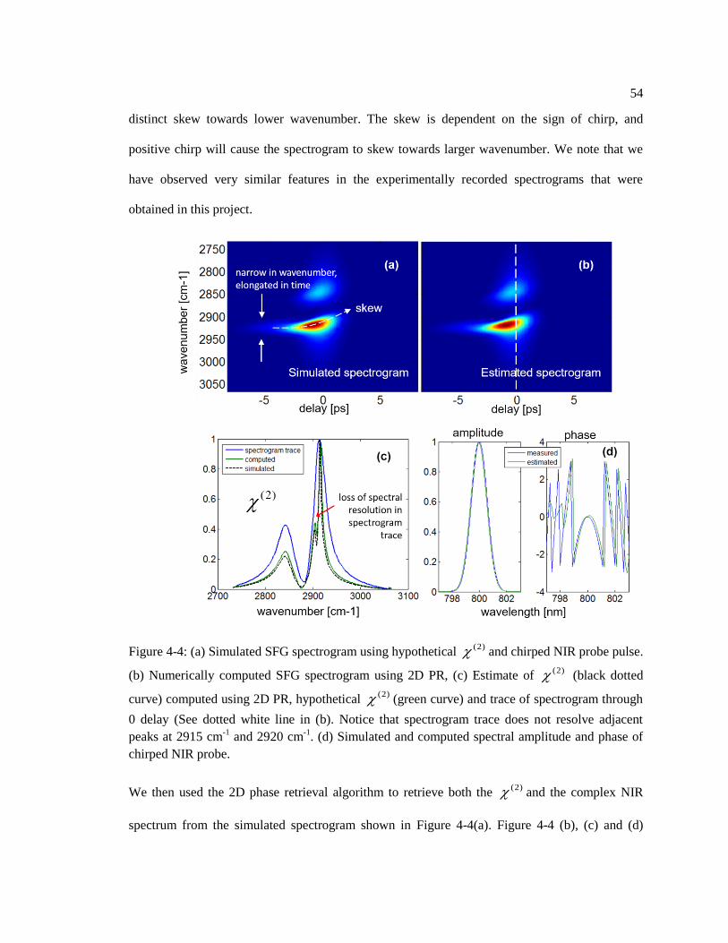
54

distinct skew towards lower wavenumber. The skew is dependent on the sign of chirp, and

positive chirp will cause the spectrogram to skew towards larger wavenumber. We note that we

have observed very similar features in the experimentally recorded spectrograms that were

obtained in this project.

Figure 4-4: (a) Simulated SFG spectrogram using hypothetical (2) and chirped NIR probe pulse.

(b) Numerically computed SFG spectrogram using 2D PR, (c) Estimate of (2) (black dotted

curve) computed using 2D PR, hypothetical (2) (green curve) and trace of spectrogram through

0 delay (See dotted white line in (b). Notice that spectrogram trace does not resolve adjacent

peaks at 2915 cm-1

and 2920 cm-1

. (d) Simulated and computed spectral amplitude and phase of

chirped NIR probe.

We then used the 2D phase retrieval algorithm to retrieve both the (2) and the complex NIR

spectrum from the simulated spectrogram shown in Figure 4-4(a). Figure 4-4 (b), (c) and (d)

55

demonstrate that we can retrieve even the asymmetric spectrogram and (2) spectrum as well as

chirped NIR pulse with high fidelity. Again, the two closely spaced peaks are clearly resolved

and we observe robust agreement between the numerically retrieved and simulated spectra of

(2) . It is clear from these simulations that our algorithm can enable high resolution SFG

vibrational spectroscopy using the conventional broadband SFG-VS. Indeed this is not surprising

and can be understood by noting the underlying physical significance of the data encoded in the

spectrogram. The spectrogram records, spectrally, the dynamics of the evolution of the

vibrational mode(s) being probed by using the relatively delayed NIR pulse, as is typically done

in time-resolved spectroscopy. This 2D dataset is partially equivalent to what would be measured

if one synthesizes an effectively much longer NIR pulse by combining the delayed copies of the

actual NIR pulse used in the experiment. However, the phase of the effectively synthesized NIR

pulse is not available with such measurement. This missing piece of information is what is

precisely estimated using the 2D PR computational technique. Thus we can not only leverage the

temporal resolution inherent in broadband SFG spectroscopy, but also recover the spectral

resolution computationally. This is the most unique feature of our technique which is in addition

to the fact that the conventional broadband SFG spectroscopy is experimentally easier to perform

than the more involved high resolution SFG spectroscopy using sophisticate pump and probe

laser systems.

Experiment

The full details of the SFG experimental setup for the air/DMSO interface studies were

previously published. [132] Briefly, the Ti:Sapphire oscillator and amplifier (Libra, Coherent,

Inc.) generates ~85 fs 800 nm pulses at 2 kHz repetition rate (2.4 mJ/pulse) and 12 nm full width

56

half maximum (fwhm). The ps NIR pulse is obtained from the 800 nm pulse by broadening it.

There are two common methods used for broadening the femtosecond pulse. In one method, a set

of two Fabry-Pérot etalons is used in series and in the second method the pulse is spatially filtered

using a combination of grating, lens and slit. Approximately 30% of the fundamental broadband

800nm output is filtered through two Fabry-Pérot etalons (TecOptics) in series to produce the

spectrally narrow (~2.1 ps) pump pulses (bandwidth Δν =13.4 cm-1

). However the use of etalons

in series is known to broaden the pulse asymmetrically with a longer tail. This causes the shape of

the SFG spectrogram to be distorted and introduces errors in the obtaining the solution using the

2D phase retrieval technique. To avoid this problem the grating and slit method is used. This

setup consists of a grating (830 groves/mm, with blazing angle of 19.7o at 820 nm), length

cylindrical lens with focal length of 100 mm, an adjustable slit, and a mirror. The grating

spectrally disperses the pulse and the cylindrical lens focuses it into a line on the mirror. The

variable slit is placed right in front of the mirror and can be closed in order to spatially filter the

pulse spectrum, thereby broadening it. The spatially filtered reflected pulse is then picked off by

another mirror. In this way, we were able to generate pulses with variable band width by

controlling the slit width. The 800 nm power was reduced to 3mW (1.5 μJ/pulse) or 30mW (15

μJ/pulse) when the slit was opened by 2.5 or 7 μm, respectively. Polarization control was adjusted

using a combination of two half-wave plates and Glan-Thompson polarizing prism.

Approximately 70% of the broadband 800nm output is used to produce broad bandwidth mid-

infrared probe pulses tunable in the range (2.3‒10 μm), using a two stage unit (OPERA solo,

Coherent, Inc.) with optical parametric amplification (OPA) followed by difference frequency

generation (DFG) with AgGaS2 (Light Conversion, Vilnius, Lithuania). The IR pulse shape had a

Gaussian profile and the full width at half maximum (FWHM) = 130 cm-1

, which was

characterized by analysis of the SFG signal collected from the surface of α-quartz in reflection

mode. The measured output energy by pyroelectric detector of the broadband IR was 20μJ/pulse

57

in the CH stretching region (2800‒3000 cm-1

). The IR pulse was centered at 2925 cm-1

and 2940

cm-1

for the DMSO and α-pinene experiments, respectively. For sample mounting, neat liquid

solution of both DMSO and α-pinene was placed in a Teflon dish and for TIR-SFG experiments,

a 45° CaF2 window was placed covering the dish. The experimental schematic is shown in Figure

4-5.

Figure 4-5: Schematic of experimental setup (ssp configuration)

The pump and probe pulses were overlapped on the air/DMSO interface using a single CaF2

focusing lens and the broadband SFG signals were collected in the momentum conserved

direction. Thus the incidence angles for all beams were ~45° with respect to the surface normal.

This geometry gives simple alignment between the reflection and total internal reflection (TIR)

modes as well as simple alignment of the invisible SFG beam into the detector slit (50μm) using

the reflected 800nm beam. The polarization combination for all experiments was ssp, (s-polarized

SFG, s-polarized pump and p-polarized probe). For acceptable signal to noise ratio, each

spectrum was collected with a 10sec exposure time and 4 spectra were arithmetically averaged

together and normalized from the SFG signal taken from the surface of α-quartz. Collection of

spectra using different time delay between 2 ps and 85 fs pulses was performed by moving the

58

motorized delay stage at 100fs scanning steps in a total range of ±6.4ps. The SFG signals were

dispersed by a holographic imaging spectrograph, 2.1cm-1

/pixel (Holospec) and recorded with a

CCD camera (iDuS 420A, Andor) which has 1024x256 active pixels.

Results and Discussion

We now show the results of using two dimensional phase retrieval for retrieving the

(2) spectrum of air/DMSO interface from its SFG spectrogram. Figure 4-6(a) shows the

experimentally measured spectrogram acquired by recording the spectrum as the NIR probe is

delayed with respect to the IR pump by a range of delays from 6.4 ps to 6.4 ps.

Figure 4-6: Match between experimentally recorded and computationally retrieved SFG

spectrogram of air/DMSO interface. (a) Recorded BB-SFG SFG spectrogram of the air/DMSO

interface taken in the range of ±6.4 ps delay between the 2 ps probe pulse and broadband pump

59

pulse at ~3.4 μm. (b) Numerically estimated BB SFG spectrogram using 2D PR. (c) Trace of

spectrograms when both pump and probe overlap with no delay. (d) Trace of both spectrograms

along peak of the spectrum.

Using the recorded spectrogram and the mathematical model of SFG process as the two

constraints, the generalized GS algorithm begins with a generic guess for the spectral form of

(2) and iteratively updates the guess to converge to the estimated spectrum of (2) . The NIR

pulse spectrum is experimentally measured separately and is used in the numerical reconstruction

of the spectrogram in each step using the update guess for (2) spectrum. The mismatch between

the numerical reconstruction and the experimental measurement is defined as the error metric.

Figure 4-6(b) shows the spectrogram after the algorithm has converged. The excellent agreement

between the two spectrograms can be seen from Figure 4-6(c-d) which compare the line traces

through the center of both spectrograms along wavenumber and delay axis respectively. To

further verify that algorithm does indeed converge to the closest solution, Figure 4-7(a) tracks its

performance by plotting the error, and shows convergence in under 20 steps in the case of single

peak for air/DMSO interface. Figure 4-7(b) shows the estimated (2) spectrum, and a Gaussian

fit to it.

60

Figure 4-7: (a) RMS error between measured and computed spectrograms. (b) Estimated (2)

spectrum of air/DMSO interface

It shows a linewidth of ~8.7 cm-1

for the 2925 cm-1

DMSO line. This agrees very well with the

recently reported linewidth of ~8.8 cm-1

using the experimentally sophisticated HR-BB-SFG-VS

technique for the same line. In contrast to this, we also show the line trace of the measured

spectrogram along zero delay, i.e. the SFG spectrum when the pump and probe overlap with no

delay. This spectrum has linewidth of 10.95 cm-1

, in other words it is ~26% broadened than the

true linewidth due to the effect of the ~2 ps long NIR pulse. It is clear from these results that the

computational 2D PR technique is capable of recovering the high resolution spectrum from low

resolution measurements typical of conventional broadband SFG spectroscopy. This capability is

inherent in the fact that the 2D SFG spectrogram dataset is effectively equivalent to that obtained

by using a much longer probe which may be synthesized using the relatively delayed copies of

the actual probe. By recovering the phase information, our technique enables broadband SFG

vibrational spectroscopy to capture the vibrational dynamics with high temporal and high spectral

resolution simultaneously. In addition, our computational technique retains the experimental

simplicity of the conventional broadband SFG spectroscopy and thus potentially enriches the

existing research initiatives in the field of surface and interface studies using SFG spectroscopy.

61

Spatio-temporal characterization of ultrashort optical pulse

Introduction and motivation

Accurate characterization of ultrafast optical laser field is important for many

applications of scientific and technological interest since it can provide insight into the temporal

and even spatial dynamics of the pulse as it interacts with its environment. One can imagine that

such knowledge can be critical in many applications. For example, Figure 4-8 shows a

hypothetical scheme which depicts change in a femto-second (fs) pulse shape which may occur

due to some process such as light matter interaction. Precise knowledge of the amplitude and

phase of the fs pulse in both space and time before and after the process can help analyze the

process in terms of the change in the pulse behavior.

Figure 4-8: Schematic depicting change in fs pulse due to its interaction within a hypothetical

process. Ultrafast pulse characterization can accurately measure amplitude and phase of fs pulse.

The capability of characterization of ultrashort pulse is important in several fundamental studies

which involve dynamic pulse synthesis and pulse shaping to influence light matter interaction.

[133] It can aid in fundamental science by providing guidance for synthesis of ultrashort pulses to

enable spatio-temporal control of lattice vibrational waves [134], to influence molecular

dynamics by enabling single-molecule control and manipulation [135]–[137] and to realize

coherent control of photons [138] to achieve local field enhancement [139] and spatio-temporal

62

control on femtosecond time and nanometer length scale [140]. Similarly, knowledge of the

ultrafast optical pulse can aid laser performance diagnostics [141], [142] and help tailor the

excitation to optimize nonlinear microscopy [143]. Moreover we find applications in which the

spatial distribution of optical field is not the same for all frequency components, i.e.,

( , ) X( ) ( )E r r where ( , ) F.T. ( , ) ( , ) i tE r r tE E r t e dt and F.T. stands for

Fourier transform. As a simple example, coupled spatio-temporal evolution of ultrashort field can

be observed in diffraction and dispersion effects of lenses, and as a result the pulse can have a

complicated profile near the focus. Multiple scattering of coherent pulsed light through thick

strongly scattering media may also exhibit non-trivial wavelength dependent speckle pattern

[144]. Dynamic coherent control of surface plasmon polaritons in nanometer femtosecond regime

has been demonstrated by controlling the phase of the coupled spatio-temporal field [145]. It is

well-known that for plasmonic systems with both nanoscale modal distribution (i.e., hot spots) as

well as a large plasmonic resonance the spatio-temporal dependence of the ultrafast electric field

cannot be decoupled. Therefore it is necessary to develop techniques to characterize the spatio-

temporal evolution of ultrashort optical pulse.

Frequency resolved optical gating and 2D phase retrieval

The fundamental dilemma of characterization of the femtosecond pulse, which can be as

short as only a few cycles long, by sampling was a daunting challenge until recently because

ultrafast pulses are some of the fastest transient phenomena themselves. The Wiener-Khinctine

theorem relates the pulse spectrum to its autocorrelation via the Fourier transform, but it cannot

uniquely determine the phase; this is the 1D phase retrieval problem we have seen in chapter 3.

Similarly intensity auto-correlation only yields a measure of the pulse width but fails to reveal the

63

complex pulse shape. Trebino and co-workers pioneered the non-linear technique of frequency

resolved optical gating (FROG) [146] by combining the measurement of autocorrelation and

spectrum to generate the pulse spectrogram. FROG has been described as an auto-correlator type

measurement in which the auto-correlator signal beam is spectrally resolved. In fact the pulse

spectrogram is similar to that seen in sum frequency generation spectroscopy. If we take the

example of a very common FROG measurement modality, namely second harmonic generation

FROG, then the SHG-FROG signal is generated by gating the unknown pulse

0( )ex( ) pi t

EE t t

with itself at variable delay times in a 2nd

order non-linear optical crystal

and the generated second harmonic signal is recorded spectrally for each delay. Thus the SHG-

FROG spectrogram is given as 2

( ) ( , )exp(, )FROG sigI E t ti dt where

( , ) ( ) ( )sig E EE t t t . Thus if there exists a unique way to obtain ( )E t from ( , )sigE t , then

the 2D PR problem can be found readily applicable to the problem of pulse retrieval using the

FROG spectrogram. In particular, the functional form of ( , )sigE t and the measured intensity of

the FROG spectrogram act as the two constraints for the iterative GS algorithm, which upon

convergence can determine the ultrafast pulse uniquely up to some trivial ambiguities (which we

will describe in next paragraph). Thus FROG is a 2D PR based technique for measuring the

amplitude and phase of typical ultrafast pulses and indeed there is a sizeable body of work in this

field [36].

Spatio-temporal characterization of ultrafast pulse

The conventional FROG technique has a few important limitations. FROG obtains the

complex pulse shape of the “whole beam” by assuming that an ultrashort optical field can be

64

separated into a spatial distribution multiplied by an independent temporal evolution function

( ), ( ) ( )rE r . We have seen above that this assumption is clearly inconsistent with

several applications due to phenomena such as wavelength dependent dispersion, diffraction and

scattering. Since SHG-FROG trace is related to the pulse auto-correlation in which the pulse

gates itself, the inherent symmetry results is time ambiguity: i.e. the field

0( )

0 0( ) ( )i t t

t t A t t eE

for some arbitrary time shift 0t , and the time reversed field

( )( ) ( ) i tt A tE e will also generate the same FROG trace. To overcome these limitations

and enable coupled spatio-temporal characterization, several techniques based on the concept of

spectral interferometry have been proposed. Spatiotemporal characterization of ultrashort pulses

has been demonstrated by spatial-spectral interference (SSI) [147], [148]. SEA TADPOLE [149]

and STARFISH [150], [151] are experimentally simpler implementations of SSI technique using

optical fibers. Dorrer et al. [152] reported a technique combining SPIDER with spatial shearing

interferometry for measuring both the spectral and spatial phase. STRIPED FISH [153] is a

holographic method for single shot measurement of three-dimensional spatiotemporal electric

field by recording spatially separated array of quasi-monochromatic holograms. NSOM probes

may be used with SEA TADPOLE [154] or other techniques to improve spatial resolution.

However, existing NSOM probes have limitations as they require converting local non-

propagating field into radiating field traveling in free space or in the NSOM fiber, which could

potentially lead to perturbation of the local field itself and hence inaccuracy for measurement at

nanoscale. Nano-FROG [155] achieves high spatial resolution using individual second harmonic

(SH) nanocrystal clusters dispersed on a substrate; however the presence of the substrate inhibits

near field measurements. Multi-pulse Interferometric FROG (MI-FROG) which combines FROG

and spectral interferometry is capable of single shot characterization of electric field consisting of

multiple ultrashort pulses and obtaining the relative phase and the temporal offset between the

65

pulses [156]. Previously, our group has developed a new class of Second HARmonic nano-Probes

(SHARP), consisting of second harmonic nanocrystals attached to carbon nanotubes which are in

turn attached to tapered optical fibers [157]. Using SHARP-based collinear FROG (CFROG)

measurements, our group has demonstrated the capability to characterize ultrashort optical fields.

However, SHARP probes lack a phase reference to coherently link the optical pulse characterized

at multiple locations. Critical information such as phase velocity and group velocity therefore

cannot be retrieved.

Here, we introduce holographic FROG, a novel technique for spatio-temporal

characterization of ultrashort optical field by combining FROG and spectral holography [158]. In

FROG holography, the use of reference beam at the SH wavelength establishes a phase coherent

link which makes it possible to measure the spatio-spectral phase of the pulse at multiple

locations. In the following, we first discuss the theory of FROG holography. Next we present a

numerical simulation to illustrate pulse retrieval at each location from the holographic FROG

trace. Finally we present an experimental study to demonstrate the measurement of group delay

of the pulse, which is not possible using the conventional FROG technique.

Formulation

Our technique of holographic FROG is designed for spatiotemporal characterization of

the ultrashort optical field. To do this, we propose to interferometrically detect the collinear

FROG (CFROG) signal by using a reference beam at the SH frequency as a local oscillator. Let

us consider the field 0( , e( , ) ) xpi t

r E r tE t

at location r , where ( , )( , ) ( , ) exp i r tE r t I r t

is the complex amplitude, ( , )I r t is the intensity, and ( , )r t is the phase, and 0 is the center

angular frequency. Also, consider the SH reference pulse 02( ) ( )exp ,

tSHG SHG i

R RE t tE

where

66

( )SHG

RE t is its complex amplitude. The corresponding holographic CFROG (HCFROG) trace is

given by:

2

2,( ) F.T. ( ) ( ) ( ), , , SHG

HCFRO RG r r tI E Er tE t

(0.17)

where is a proportionality constant. Let 02 . We define the following:

2( , )F.T. ( ),,SHGE r t E r ( , ) ( , )F.T. 2 ( , ),FROGE r t E Er t r and

F.T. ( ) ( )SHG

R Rt EE . Eq. (0.17) can then be rewritten as

0

0

2

2

( ) | ( ) ( )

( ) (

,

)

,

|

, ,

, ,

ii

HcFROG SHG SHG

i

FROG R

I E E e e

E

r r r

e Er

(0.18)

The holographic term of interest in Eq. (0.18) is 0 *, , ,) ( ) ( ),( R

i

FROGr E rH e E .

Algorithm

Our algorithm to retrieve the ultrashort pulse profile from its HCFROG trace is designed

to track the phase as the pulse evolves spatially. We illustrate the algorithm by considering a

numerical simulation of ultrashort pulse retrieval as it propagates through a hypothetical

dispersive medium, a schematic of which is shown in Figure 4-9(a). A typical simulated

HCFROG trace and its 2D Fourier transform (F.T.) is shown in Figure 4-9(b) and Figure 4-9(c)

respectively. The characteristic fringes of HCFROG trace are clearly seen along both wavelength

and delay axis. The 2D F.T. clearly identifies the HCFROG term, i.e. the 2D F.T. of

0 *, , ,) ( ) ( ),( R

i

FROGr E rH e E , which can be digitally filtered.

67

Figure 4-9: Numerical simulation. (a) Schematic of simulated experiment. (b) Typical simulated

HcFROG trace. (c) 2D F.T. of HcFROG traces at locations ‘P1’ and ‘P2’. r is the spatial

separation between the two locations and gv is the group velocity through the hypothetical

medium. (d) Relative FROG phasor of the pulse at ‘P2’ with respect to ‘P1’.

In our simulation of the hypothetical dispersive medium, the two points P1 and P2 at which the

HCFROG trace is measured are separated by 5 um. Although their 2D F.T. traces appear similar,

we note that the time offset of the holographic sideband corresponds to the spatial separation of

the two locations, and hence the HCFROG trace encodes the spatial evolution of the ultrashort

pulse. Indeed, the ratio of ,( ),rH at ir and jr yields the relative FROG phasor

, (( ) ,, , )( , )/i FROGFROG ij ji r r i ri r

e e e

(0.19)

where ( , , )FROG r denotes the phase of , ,( )FROGE r at r . We note that the reference field

and its delay are maintained fixed and hence it does not need to be characterized independently.

We set ‘P1’ as “pivot”, pivotr and Eq. (0.19) is used to compute the relative FROG phasor at ‘P2’

(and every other location) with respect to pivotr (see Figure 4-9(d)). We obtain the standard

background-free SHG FROG spectrogram by filtering the d.c. term and apply the conventional

68

2D phase retrieval FROG algorithm to retrieve the pulse profile at pivotr . In particular, the

conventional FROG algorithm computes the time-domain FROG trace

( ,, ( , ( )) ) ,pivot pivot pivotsigE r E r t E r tt via 1D I.F.T. of the SHG FROG spectrogram. We

normalize it by noting that ( , ) ( , ) ( , , )sigE r t d E r t dt E r t dtd so that

( , )( , , )

, ( , ) e) p( , )

( x,

pivotsig pivoti r t

pivot pivot

sig pivot

E r t dE r t I r t

E r t dtd

(0.20)

is used as the guess for next iteration, until convergence is reached. At ‘P2’, the corresponding

SHG FROG spectrogram , ,( )FROGI r and the relative FROG phasor ,( )pivoti r r

e

(computed

using Eq. (4.7)) is used to obtain the complex spectrogram

( ), ,( , )( ), , pivot FROG pivoti r r i r

FROGI e er

. Then the pulse profile at ‘P2’ is retrieved by simply

following the prescription of Eq. (0.20). In this way the spatial and temporal characterization of

the ultrashort pulse is performed by holographic FROG technique. Amongst the salient features

of our technique, we note that ,( ),rH is linear in , ,( )FROGE r and the homodyne

detection increases sensitivity to ‘weak’ spots in the spectrogram. The iterative phase retrieval is

applied only to the “pivot” location (which may be arbitrarily chosen in principle) whereas pulse

retrieval at every other location involves a single F.T. and basic algebraic operations to make use

of the phase information inherent in the corresponding HCFROG trace. This adds minimal

computational overhead to the overall pulse retrieval algorithm.

69

Numerical Simulation

We demonstrate the validity of our algorithm by a simple numerical simulation based on

the same schematic shown in figure 2. We consider the propagation of transform limited

Gaussian pulse2 2

0/( )

tA e

at 850 nm through a hypothetical dispersive medium characterized

with a group delay dispersion parameter 31133 /0D ps nm km 2 2'' 51( 512 0 / )k s m .

The pulse has full width half maximum (FWHM) of 0t = 37 fs at ‘P1’, which is taken as the pivot

location in this simulation. The positively chirped pulse profile can be computed at any location

within the medium using 2 ' 2

0(1 ')( / )( , )

ia tA z e

where ' / da z L and

2'

0 0 1 / dt t z L [23].

For this simulation, ‘P2’ is 5 um and ‘P3’ is 15 um from ‘P1’.

70

Figure 4-10: Results of numerical simulation using HCFROG algorithm (a) retrieved and

theoretical complex pulse profile. FWHM is marked for pulse at each location. (b) computed

spatial separation between the 3 locations compared with actual separation used for simulation.

The table lists the actual values of spatial separation as used in the numerical experiment and

retrieved using method described. (c) comparison of retrieved and theoretical pulse spectrum at

each location. FWHM is marked for the pulse spectrum. (d) comparison of retrieved and

theoretical SH spectrum of pulse at each location. FWHM is marked for the pulse spectrum.

71

Figure 4-10 shows the comparison between the pulse profiles retrieved from the HCFROG trace

at each location by using the algorithm discussed above, with the corresponding theoretical pulse

profiles. The pulse amplitude (including FWHM) and quadratic phase profiles (due to positive

chirp) agree with their theoretical profile at each location Figure 4-10(a)). The minor deviation

from flat phase for the pulse at ‘P1’ is attributed to numerical errors due to discretization.

Similarly the retrieved pulse spectrum (Figure 4-10(c)) and its SH spectrum (Figure 4-10(d)) also

agree well with the theoretical profiles at each location. We obtain the relative spectral phase of

the pulse between each location , ,( , ; ) ( ) ( )i ji j r r using the retrieved pulse profile

at each location. The group delay of propagation through the medium can be obtained by

computing the gradient ( /, ; )g id dj of the relative spectral phase between any pair

of locations; and the separation between those locations is obtained by g gv . Figure 4-10(b)

plots the spatial separation thus computed numerically compared to the actual separation used for

the simulation, and the included table lists the actual values in microns. The comparison in all

result panels is very solid. This clearly shows that the HCFROG trace records the carrier phase

and group delay of pulse propagation, i.e. the first two terms in the Taylor series of the spectral

phase 2

0 0 0( , ) ( , ) ( , ) 0.5 ( ) ...,r r r r in addition to the O(2) terms

that are measured by conventional FROG (aside from an overall undetermined constant).

Experiment

As a proof-of-concept demonstration of our HCFROG technique, we in situ characterize

the pulse near the focus of an objective lens, by using a BaTiO3 micro-cluster air-dried on a cover

glass as the nonlinear probe and traversing through the focus of the objective along its axis. As

shown in the setup in Figure 4-11(a), a Michelson interferometer with a variable delay arm

72

generates two copies of the fundamental pulse which is obtained from a Ti:Sapphire laser

(KMLabs, central wavelength ~818nm, average output power ~400mW, repetition rate 88MHz).

The two pulses combined at the output of the interferometer first propagated through a short

length (~10cm) of photonic crystal fiber before being focused on the BaTiO3 micro-cluster by a

40 objective lens to generate the SH CFROG signal. An SEM image of the micro-cluster is

shown in Figure 4-11(b). We vary the delay in steps of 0.4 fs which is enough to satisfy the

Nyquist sampling rate for the CFROG signal, although it has been shown that the delay step may

be increased to speed up acquisition without affecting the final retrieved pulse [159]. In our setup

we have mounted the PCF output end and the collimating and focusing objectives on the same

translational stage (as indicated in Figure 4-11(a)). This arrangement effectively allows us to

probe the focused femtosecond beam at multiple locations along the objective axis without the

need to move the micro-cluster itself or the signal acquisition optics, thereby maintaining the

optical path of generated CFROG signal. Additionally, a SH reference pulse (~409nm) is

generated from the fundamental beam by using a Barium Borate (BBO) crystal, separated by a

dichroic filter, and appropriately delayed to interfere with the CFROG signal. The resulting

HCFROG trace is filtered by a band-pass filter (D400/70, Chroma Technology) and detected by a

spectrograph (PI Acton SP2500i with a liquid nitrogen cooled charge coupled device camera,

resolution: 0.03nm at 409nm). Figure 4-11(c) shows a typical recorded HCFROG trace which

exhibits the characteristic fringe structure along both the delay and wavelength dimensions. We

acquire such HCFROG traces at five locations as we traverse through the focus: ‘location 2’ at

9.43 μm, ‘location 3’ at 18.11 μm, ‘location 4’ at 27.37 μm and ‘location 5’ at 37.75 μm with

respect to the pivot ‘location 1’.

73

Figure 4-11: (a) Schematic of our experimental setup. (b) The inset shows SEM image of the

BaTiO3 micro-cluster used for generating FROG signal. (c) Typical recorded HcFROG trace.

The fringe structure can be seen along both delay and wavelength dimension.

Results and Discussion

We implement the procedure described in section 2 to retrieve the complex pulse profile

from the recorded HCFROG trace. In our experiment, among the five locations at which

HCFROG trace is acquired, the ‘pivot location’ is chosen to be closest to the focusing objective

along the axis. As noted in Figure 4-11(a), ‘location 4’ is nearest to the focus. First panel in

Figure 4-12(a) shows the intensity and phase of the pulse at pivot location retrieved by applying

the conventional FROG algorithm at that location. The full width at half maximum (FWHM) of

the retrieved pulse is 89 fs (at temporal resolution = 4 fs). At other locations, the relative FROG

phasor with respect to pivot is computed as prescribed by Eq.(0.20). Combining the relative

FROG phasor with the FROG trace (extracted digitally from the corresponding experimentally

measured HCFROG trace at that location), the resulting complex spectrogram can be simply

inverse Fourier transformed and processed to obtain pulse amplitude and phase at that location, as

described before.

74

Figure 4-12: Pulse characterization at multiple locations using FROG holography. (a) Retrieved

pulse profile (amplitude and phase, FWHM ~89 fs) at each position; (b) Comparison of both

fundamental and SH power spectrum of the retrieved pulse at each position with measured power

spectra (black squares) (FWHM ~12 nm) (c) Comparison between retrieved and experimentally

recorded spatial separation between each location with respect to pivot. The table in inset lists

actual values in m .

75

The panels in Figure 4-12(a) show pulses retrieved at each location. The pulse generally

maintains its amplitude profile, displays slightly different phase profile, and is shifted along the

time axis in accordance to the separation of the spatial locations as it travels along axis through

the focus. To check the validity of the retrieval process, in Figure 4-12(b) we compare the

measured laser spectra (both fundamental and at SH) with that computed from the retrieved pulse

profile at each location. The measured and computed spectra agree reasonably well and do not

vary significantly between the five locations. The FWHM bandwidth of the fundamental pulse

spectrum is ~12 nm. Further we computed the spatial separation between each of the locations

using the derivative of the relative spectral phase as was discussed in the simulation section.

Figure 4-12(c) and the table within show the comparison between numerically obtained and

experimentally measured distances from the pivot to every other location. The agreement not only

validates our retrieval procedure but also serves as proof-of-concept demonstration of the

potential of FROG holography to fully characterize the spatiotemporal evolution of an ultrafast

optical field.

Conclusion

In summary, our technique of FROG holography utilizes a reference beam to record

spectral holograms of conventional CFROG traces at multiple spatial locations. In contrast to

other existing techniques, our method does not require the reference beam to be characterized, as

long as it stays stable during the entire measurement. We have shown that it contains not only the

standard non-collinear FROG term but also the relative FROG phasor and thereby coherently

‘links’ the measurements at different spatial locations. We have discussed a method to retrieve

the complex pulse profile from the recorded HCFROG traces, and demonstrated the measurement

of group delay of the pulse in the vicinity of the focal point of an objective lens. In short, FROG

76

holography combines high sensitivity of spectral holography with FROG to characterize the

detailed temporal phase structure of the pulse as well as provide key information about group and

carrier velocities of pulse propagation. The improved sensitivity of homodyne detection is useful

for probing “weak” spots or for increasing the scanning speed by reducing the integration time of

the spectrometer. In principle, FROG holography makes it possible to measure the spatio-

temporal evolution of complicated ultrashort pulse that can be characterized by the general FROG

technique. In combination with nonlinear nanoprobes [157], FROG holography has the potential

to image the spatiotemporal evolution of ultrafast optical fields in femtosecond time scale and 3D

nanometer length scale, which could benefit emerging applications in biomedical imaging,

plasmonics, and metamaterials.

77

Chapter 5

Summary and Future Prospects

We have presented a few examples in imaging and spectroscopy in which the application

of computational methods has enabled enhancements and helped overcome limitations in existing

techniques. Compressive coherent anti-Stokes Raman holography was shown to enhance the

apparent optical sectioning capability of image reconstruction using digital holography. This

capability enriches the existing label-free chemical selectivity and non-scanning 3D imaging

features of coherent Raman holography. This can be further improved by using the beam

propagation method which accounts for non-uniform propagation medium and potentially extend

this capability for 3D imaging in the presence of scattering elements using single hologram. Our

proposed compressive frequency comb spectroscopy technique can in principle achieve sub-

picometer resolution across tens of nm of broad spectral coverage. Such ultra-high resolution can

enable molecular fingerprinting and accurate spectral assignment to help identification of

unknown species. The current research in development of stable and miniaturized frequency

comb will undoubtedly help the development of ultra-high resolution optical metrology in

general, and our spectroscopy technique provides an example of efficient optical sensing

applications based on compressive sensing. Non-linear optical spectroscopy such as sum-

frequency generation spectroscopy has advanced the science of surface chemistry by enabling

non-invasive, non-destructive optical probe with excellent intrinsic molecular specificity and

surface selectivity. Our computational technique based on two dimensional phase retrieval for

SFG-VS enhances the spectral resolution achievable using the most commonly implemented

conventional experimental procedure thereby providing simultaneous high temporal and spectral

resolution insight for analyzing different molecular species at the surface of media. All these

applications employ specialized pulsed laser sources, especially ultrafast femto-second lasers and

78

as such it can be important to characterize the spatio-temporal dynamics. We have developed a

sensitive technique which combines the existing FROG technique with spectral holography to

help overcome some key ambiguities in conventional FROG and enable characterization of the

spatio-temporal evolution of the ultrashort pulse. In particular, the capability to measure the

group delay could significantly enhance imaging modalities based on time of flight imaging by

providing femtosecond resolution. Additionally, the potential of our technique lies in its

capability to achieve 4D imaging of the ultrafast field ( , , , )E x y z t with nanometer spatial and

femtosecond temporal resolution, in essence nano-femto microscopy.

79

Appendix A

Opto-electronic nano-probe

In this appendix, I report on a project which was done based on support of NSF (Grant#

1128587). It represents a substantial part of my overall output during PhD. Hence I have opted to

include a report of the project in the appendix to my thesis.

Introduction and Motivation

The field of fiber optics has witnessed significant advances owing to the pioneering work

of Russell and coworkers which has led to the development of micro-structured optical

fiber,[160]–[162] in particular photonic crystal fiber (PCF). An important advantage of PCF over

conventional optical fiber is the ability to precisely engineer the optical modal properties by

designing the shape, size and distribution of the air holes. The recent active scientific interest can

be attributed to the fact that the properties of PCF can be altered by incorporating special

materials in its air holes. Indeed, the choice of material(s) and selective filling of air holes offer

additional degrees of freedom which vastly expand the scope of PCF based optical devices and

their applications. Of particular interest here is the fact that electrically conductive media, such as

metals, may be filled in the PCF structure to design novel devices and sensors. For example,

Sazio et al. demonstrated unique all-in-fiber active photonic devices [163], [164] by filling silicon

and germanium within the air holes. Recently several applications based on filling metals in PCF

have been reported.[165]–[169] Furthermore, surface plasmon polariton sensors based on metallic

filling of PCF has also been the focus of active research.[170], [171]

Metal filled PCF devices feature the ability to conduct electricity as well as guide optical

waves. Furthermore, nanotubes or nanowires can be incorporated within metal filled PCF such

80

that each nanoprobe may be individually controlled. This points to the exciting potential of

developing an integrated opto-electronic fiber platform which is capable of simultaneous

electrical and optical interrogation and probing at the nanoscale. Key to developing such a

platform is the ability to repetitively and reliably fill metal into the air holes of the PCF

selectively without damaging its structural integrity or its optical wave-guiding functionality.

Towards that end goal, here we report on the fabrication and characterization of a novel fiber

based opto-electronic nanoprobe engineered by selectively penetrating metal electrodes in PCF

and by attaching nanotubes individually to each electrode. We present methods to create any

desired configuration of such electrodes and show the feasibility that the attached nanotubes can

be actuated through electrostatic force by controlling the voltages applied to the electrodes. In

other words, the PCF serves as scaffold for an electromechanical nanoprobe as well as an optical

waveguide. This unique aspect of our device differentiates it from existing single tip

nanomanipulators [172]–[175] and two arm nanotweezers. [176]–[179]

The report is organized as follows: we begin by presenting the techniques we have

developed for fabrication of the proposed opto-electronic nano-probe, including selective filling

of metal electrodes in PCF and precise attachment of individual nanotubes to them. We then

report results of optical characterization of our device using spectral holography to quantify the

group velocity dispersion of the metal-filled PCF. Lastly we discuss the potential

electromechanical functionality of the device by demonstrating the feasibility of electronic

actuation of the attached nanotubes, and comparing the observed movement with numerically

simulated deflection.

81

Selective filling of PCF

Selective penetration of foreign material especially metals in air holes of PCF has led to

design of novel fiber devices optimized for particular applications. A wide variety of techniques

have been demonstrated to achieve selective filling. Some of the early techniques for infiltrating

metal involved carefully inserting thin metal wires directly into specific fiber air holes [180] and

using vacuum suction [181] to draw molten material into the fiber.

Huang et al. leveraged non-uniform air hole sizes in their multistep injection-cure-cleave

technique to demonstrate selective filling of larger diameter holes with a UV curable polymer by

applying external pressure.[182] Another technique based on varying size of air holes involves

use of fusion splicer to collapse smaller holes and leave open larger holes for filling. [183], [184]

Borrowing on the technologies developed in the field of microelectronics, a novel technique

based on use of high pressure chemical vapor deposition was developed to successfully

demonstrate filling of semiconductors and metals to form functionalized MOF fiber

devices.[163], [185] It has also been shown that the conventional stack and draw procedure can

be adapted to fabricate PCF with appropriately positioned stack of metal rods around the core,

instead of penetrating the PCF post fabrication. [186] Vieweg et al. have shown selective filling

of PCF in arbitrary pattern by targeting and sealing individual air holes using a focused pulsed

laser to polymerize a photo-resist covering those holes, so that the unsealed holes are available to

be filled. [185] Another method utilizes side access to the air holes through the fiber walls created

using focused ion beam, so that the process of selective filling does not occlude optical access to

the PCF facet. [187] In our technique detailed below, we selectively pattern the PCF facet by

targeted application of UV curable optical glue to individual air holes, followed by pumping

molten metal in the open holes under high pressure. In fact, variants of the technique of using

pressure differential to pump or draw molten metal into PCF has been reported by several

82

researchers in the past. [165], [166], [169], [188]–[190] Our procedure does not require the air

holes to be of varying size, and is not influenced significantly by fluidic properties of the liquid

phase metal. It does not involve milling/splicing/arcing or other steps which may cause damage

and alter the optical properties of the PCF. This ensures that the fiber can guide light and

electricity along its length and perform both electrical and optical probing as envisaged above.

We demonstrate our procedure, illustrated in Figure A-1, by filling multiple individual holes in

more than 15 inch long endlessly single mode PCF (SC-PCF, Blaze Photonics ESM-12-01) with

low melting point metal.

Figure A-1: Schematic illustrating patterning of PCF for selective filling

The fiber has a 12 µm solid silica core surrounded by hexagonal array of 3.68 µm air holes in

cladding region. The pitch of cladding holes is 8 µm. As shown in Figure A-1(1), initially the

three holes to be infiltrated are each sealed by local application of a drop of UV-curable optical

glue (NOA-81) under an optical microscope using a fiber taper maneuvered with a three-axis

stage. Upon curing, the selectively blocked facet of the PCF is immersed into NOA-81 which

draws the glue into all but the blocked holes at least 5-6 mm deep via capillary action (blue

83

column in Figure A-1 (2) and (3)). Further UV curing of the penetrated optical glue, followed by

cleaving the PCF close to the facet creates the required PCF template with only the three holes

exposed (Figure A-1(3)) as desired. The PCF template is then mounted within a home-made high

pressure pumping system for pumping molten metal through it. In particular, the patterned facet

of the fiber is held in place in a chamber using polydimethylsiloxane (PDMS) (Dow Corning

Sylgard 184 and curing agent 10:1 ratio). The chamber is topped off with Ostalloy 158 (eutectic

solder alloy of 50% bismuth, 26.7% lead, 13.3% tin and 10% cadmium, having melting point 70

°C) and is placed inside an oven which is maintained at a temperature above the melting point

(approximately 100 °C). The inset in Figure A-2(a) shows the cutout of the chamber with the

fiber facet sunk in the alloy. The other facet of the fiber is held outside the oven at room

temperature as shown in Figure A-2(a). After the temperature within the oven equilibrates,

compressed nitrogen gas at pressure of about 500 psi is used to pump the molten alloy through

the unblocked holes of the patterned fiber, until the molten alloy leaks through from the other end

which is seen as a shiny blob in the image in Figure A-2(b). This indicates penetration of the

metal along the entire fiber length and typically takes a few minutes for our nearly 15 inch long

fiber. It has been reported that pumping liquefied metal by applying pressure often causes air gaps

along the length of the filled metal due to the difference in the thermal expansion coefficient of

the metal and silica [165], [166] In contrast, our technique of maintaining the distal end of the

fiber at room temperature causes the leaking alloy to solidify into the shiny blob which then acts

as a plug to seal the channel and avoid any voids as the alloy stays compact while cooling down

under constant pressure. The selectively filled fiber is seen in the scanning electron microscope

(SEM) image in Figure A-2(c) with arrows pointing to alloy-filled holes. We have successfully

fabricated several dozens of such long selectively filled PCF containing multiple 3.68 µm sized

alloy electrodes with high yield. We further confirmed the electrical continuity of each filled

electrode by measuring the resistance between the two ends at the fiber facet by using a pair of

84

tungsten probes as illustrated in Figure A-2(d). A 4cm long piece of the filled fiber electrode

typically has measured d.c. resistance of 1657 . Based on the reported conductivity of the alloy

of 2.320 x 106 S/m, the computed resistance of 1621 agrees well with our measured d.c.

resistance. We note that following this method, we have also successfully patterned PCF with

indium electrode which melts at higher temperature of 156.6 °C.

Nano-tube attachment

As stated earlier, the proposed opto-electronic nanoprobe is designed to allow

electromechanical probing at the nanoscale in addition to functioning as an optical waveguide. It

is well known that carbon nanotubes (CNT) have several unique electronic and mechanical

properties which make them suitable for this purpose. Multi-walled CNT (MWCNT) may be

either metallic or semiconducting with a variable band-gap based on their chirality and diameter.

CNTs can carry high currents without heating and are stiff and exceptionally strong. [191] Owing

to their properties, CNT has been used in variety of applications as tweezers or probes. [175],

[177], [192]–[194] In this section, we discuss our results with two different techniques of

attaching CNT to the selectively filled PCF for fabricating our device.

85

Figure A-2 Pumping molten alloy through patterned PCF. (a) Schematic of oven showing a PCF

held in a chamber. The inset shows cutaway of the chamber in which patterned pcf is held using

PDMS and sunk in bath of alloy. (b) Filled PCF under 500 psi showing alloy leaking out as shiny

blob from the other end held outside the oven at room temperature. (c) SEM image of a pcf with

three holes filled with alloy, (d) Setup for checking electrical continuity and typical resistance of

filled electrode (1657 ohms).

We note that the non-planar, circular geometry and small, uneven cross section of the

patterned facet of the PCF precludes the use of conventional photolithography based techniques

for fabrication of our device. Additionally, the small dimension and high aspect ratio of CNT

poses unique challenges for achieving targeted attachment of individual CNT to each filled

electrode while ensuring their correct alignment. Hence, we explored and developed two separate

techniques for attaching individual CNT to each filled electrode of the fiber - (a) laser welding,

and (b) focused ion beam (FIB) and electron beam assisted deposition. In the laser welding

technique, a laser beam is steered to focus on the electrode using a 20x long working distance

objective. To prepare the CNT sample, we sonicate a dispersion of CNTs (PECVD MW-CNT

86

from NanoLab Inc. 200nm in diameter and about 20 µm long) in DI water in ultrasonic bath (Tru-

Sweep 275DA, Crest Ultrasonics), and air-dry a small drop of the dispersed solution on a glass

slide. A single CNT is then fished from the glass slide sample under a microscope using a fiber

taper and is maneuvered to a PCF electrode using multiple 3D stages while the laser is incident,

as shown in Figure A-3(a). The schematic in the inset illustrates the process from the top view.

The laser power is increased very carefully until the filled electrode melts only slightly due to

absorption of laser energy to reflow and locally weld the CNT. A gentle tug on the delivery taper

is enough to detach it from the welded CNT leaving it electrically welded with the electrode as

shown in Figure A-3(b). The same procedure is repeated for attaching each CNT to the electrode.

It is important to monitor and control the laser power carefully since the heat may melt an

adjacent electrode as well and may cause the CNT attached to it to re-align incorrectly or even

detach.

87

Figure A-3: Laser welding process for CNT attachment. (a) Side view image of CNT just prior to

being laser welded to alloy filled pcf. Inset shows the schematic top view illustrating the fiber

taper used for delivery. (b) Laser welded CNT.

The increased risk of device failure associated with the laser welding method prompted

us to investigate another technique for picking and targeted bonding of individual CNT using

FIB. In this method, the CNT dispersion is air-dried on a TEM lacie carbon grid (Electron

Microscopy Sciences LC-200 Cu). The CNT lying on the carbon mesh is attached using FIB

assisted platinum deposition (FEI Helios NanoLab 660) to a fine tungsten probe (tip size

~500nm) (7.7 pA at 30 kV) with the CNT aligned correctly (Figure A-4(a) and Figure A-4(b)). It

may be necessary to mill individual synapses of the carbon mesh which may be adhered to the

CNT as the nanotube is lifted off the grid. The tungsten probe carrying the CNT is then navigated

near the filled electrode and the CNT is bonded with the alloy using electron beam assisted

tungsten deposition (3.2 nA at 2 kV) (Figure A-4(c)). After CNT attachment the probe is milled at

its tip to release it from the CNT. We note that the fiber is coated with iridium (Emitech K575X)

88

prior to using FIB to avoid charging under ion beam. In this way, we have fabricated many

devices by sequentially attaching multiple individual CNT symmetrically around the solid core of

the PCF to individual electrodes. Figure A-4(d) shows the ion beam image of such a typical

fabricated device. We found that the yield of device fabricaton was significantly improved using

FIB owing to the controlled assembly in our pick and bond technique.

Figure A-4: FIB assisted CNT attachment. (a) CNT lying on lacie carbon mesh is bonded to 500

µm tungsten probe tip via Pt deposition. (b) CNT liftoff. Part of carbon mesh can be seen adhered

to the CNT. Individual synapses need to be milled for ‘clean’ liftoff. (c) Sequential targeted

attachment of CNT via e-beam assisted tungsten deposition. (d) Ion beam image of a three-arm

device.

Device characterization

In order to investigate the performance of the proposed opto-electronic nano-probe we

performed both numerical simulation and experimental measurements to characterize the group

velocity dispersion and electromechanical actuation. We first measured the refractive index and

extinction coefficient of Ostalloy 158 by using a rotating compensator spectroscopic ellipsometer

89

(M-2000, J.A. Woollam Co.). The alloy sample is an approximately 200 µm thin disk (shown in

inset of Figure A-5(a)) that was prepared by melting a small drop of alloy over a glass slide and

letting it reflow as it solidified on the slide. The disk was then carefully flipped over so that its

smooth and un-oxidized underside is face-up and consistent ellipsometric data was measured in

reflection geometry at multiple angles and from several locations on the disk. Figure A-5(a) plots

the averaged refractive index and extinction coefficient over 600-1400 nm range obtained from

the ellipsometric measurement.

Figure A-5: (a) The average refractive index and extinction coefficients of Ostalloy 158 obtained

via ellipsometry of the inset sample, (b) simulation of the typical optical mode field for the

unfilled PCF, (c) the mode field when three of the most center air holes are filled with Ostalloy

90

Group velocity dispersion

Using the experimentally measured conductivity of Ostalloy and the dispersion for silica

modeled using its Sellmeier coefficients, we simulated the eigenmodes and effective mode index

( )effn of the selectively filled PCF in COMSOL. Figure A-5 (b-c) shows the simulated field

distribution of the fundamental mode within the core of the bare as well as selectively filled PCF.

The presence of the electrodes in close vicinity of the core along the entire length of the fiber

slightly distorts the mode field distribution as can be seen in Figure A-5(c). The group velocity

dispersion of the PCF can be computed using 2

2

( )( )

effd nD

c d

. In this way by simulating

the effective index for both the bare as well as selectively filled PCF, we numerically obtained the

dispersion curve for each from 1.1 μm to 1.3 μm.

We also used spectral holography to experimentally characterize the group velocity

dispersion of both the bare and selectively filled PCF. Spectral holography is a sensitive and

linear optical technique to measure the relative spectral phase of the complex optical field. [195]

For spectral holography a supercontinuum source with a broad spectrum (600-1600 nm) is

generated via four-wave mixing by propagating sub-ns pulses at 1064 nm in a nonlinear PCF

(SC-5.0-1040). The reference arm of the Mach-Zehnder interferometer shown in Figure A-6(a)

consists of the supercontinuum beam delayed using a delay line. The ‘object arm’ consists of the

PCF under test. By appropriately adjusting the delay line to obtain consistent and good quality

fringes over the 1.1μm -1.3μm wavelength region, we detect the spectral hologram of the field at

the output of the PCF using an optical spectrum analyzer (Ando AQ-6315E). The spectral

hologram can be modeled as 2 2 2( ) ( ) ( ) ( ) ( ) ( ) ( ) ( )S R S R S R S R where

( )R is the reference field and )(S denotes the output field from the PCF. Typical recorded

spectral hologram is shown in Figure A-6(b). Since the spectral hologram contains information in

91

its interference fringes, the appropriate sideband of the inverse Fourier transform of the hologram

is digitally filtered, and the Fourier transform of the filtered sideband yields the complex

spectrum ( ) ( )S R . In order to remove the contribution due to the presence of other optical

components in the ‘object arm’, we additionally obtain the spectral hologram in the absence of

the fiber, and thereby calibrate the transfer function of the ‘object arm’. Taking the ratio of

processed sideband terms of these two measurements, we can acquire the complex transfer

function containing both the amplitude and the phase information of the selectively filled PCF.

Figure A-6(c) shows the typical relative spectral phase of the filled PCF. We believe that the

noise in the relative spectral phase can be attributed to the fact that the low melting point Ostalloy

is observed to exhibit plasticity during the measurement when exposed to focused laser light. This

may lead to variation in the optical path in the object arm of the interferometer. Since the group

velocity dispersion is obtained from the 2nd

order derivative of the relative spectral phase, we

smoothen the measured phase by fitting a curve with a 3rd

order polynomial in Matlab. Finally we

compute the group velocity dispersion values for D [ps/nm/km] by taking into account the length

of the fiber used in the measurement. Thus following this procedure we experimentally obtained

the dispersion parameter plot for both the bare (unfilled) and selectively filled PFC. Figure A-6(d)

shows the comparison of the numerically simulated (solid lines) and experimentally obtained

(dotted lines) curves for D for both such fibers. It also plots the manufacturer supplied data for D

for the unfilled fiber (black line). Our results show that the selective metal filling does not

damage the waveguiding properties of the unfilled PCF. In other words, the optical channel and

electric channel in our device can be accessed without affecting the performance of each other.

However we do note that the transmission efficiency of the selectively filled PCF can be

significantly lower than the unfilled fiber, especially when the holes being filled are immediately

adjacent to the central core. [169]

92

Figure A-6: Group velocity dispersion for nano-probe with 3 filled electrodes. (a) Mach-Zehnder

setup for spectral holographic measurement. (b) Typical recorded spectral hologram (c) Measured

relative phase, and 3rd

order polynomial fit, (d) estimated dispersion parameter for unfilled pcf

(red dotted) and fabricated device (blue dotted). Corresponding COMSOL simulated dispersion

for unfilled pcf (blue red line) and modeled device (solid blue line) are also plotted for

comparison. The black curve is dispersion parameter for bare fiber as specified by manufacturer.

Electromechanical characterization

The ability to control the motion of multiple nanoprobe tips allows the possibility to

mechanically interact with the sample under study as well as interrogate the sample electrically

and optically. A basic requirement of such a nanoprobe device is the ability to actuate the probe

tips to open and close them. Our proposed opto-electronic nano-probe consists of multiple CNTs

attached to each filled electrode in the selectively filled PCF. To investigate this ability in our

device, we experimentally measured the deflection of the CNT tips by applying variable potential

93

difference of up to 40V between the pair of electrodes. In particular, a pair of tungsten electrodes

was positioned in place using three-dimensional precision stages in order to contact the two

electrodes exposed at one facet of the filled PCF (without CNTs). We highlight the fact that each

electrode was independently tested for its electrical continuity by measuring its d.c. resistance as

mentioned earlier (see Figure A-2(d)). The tungsten electrodes were connected to a signal

generator to apply a manually variable dual polarity dc voltage (±20V) or generate a pure tone

sine wave of ac amplitude 40V. Thus the CNTs connected at the other facet accumulated charges

of opposite polarity and varying density as the voltage was varied and bent towards each other in

response to attracting charges. We recorded a video of this motion of the CNTs on a CCD

camera. Figure A-7(a) shows a montage of three frames in sequence from the recorded video in

which the CNT deflection is visible. The observed range of nano-tube deflection was small. To

help visualize the deflection, Figure A-7(b) plots the line trace of the image along the line marked

in each frame. We observe a deflection of the tip of the nanotubes of 2 to 3 pixels (note the pixel

numbers in the magnified Figure A-7(c)). The deflection is more pronounced in the lower CNT

than the upper (in the frame). Accounting for the magnification of our imaging system, this

corresponds to approximately 260 nm to 392 nm deflection.

94

Figure A-7: Electro-mechanical deflection of fabricated nano-probe. (a) Montage of 3 sequential

frames from a video recording CNT deflection. The dotted line shows the trace along which

intensity is plotted in (b) and (c). The markers in (c) indicate pixel positions of the ‘tip’ of the

lower CNT in each frame.

To investigate the relatively small deflection of the nano-tubes, we numerically simulated

the bending of the CNTs in a model of the fabricated device. We utilized the MEMS module of

COMSOL Multiphysics to solve the coupled physical model based on structural mechanics and

electrostatics. This involves modeling the CNT as an electrically conductive and linearly elastic

material by specifying its physical parameters including density (ρ), Young's Modulus (E) and

Poisson's ratio (ν). With the exception of the resistivity, which was measured experimentally, the

physical properties of the CNT were chosen to be in between those of graphite and multi-walled

CNTs. These values are ρ=2300 kg/m3, E=1.28 GPa, and ν=0.35 respectively. The choice of

Young's Modulus was most critical as this parameter varies several orders of magnitude (TPa to

GPa) based on the number of walls and diameter of the CNT. [196], [197] We therefore chose

the values noted above as being between those of bulk graphite and small MWCNTs. The length

95

and diameter of the CNT in the simulations were chosen to be 20 µm by 200nm as an average of

those used in the experiments. The accumulation of charge on the tips of the CNT in response to

applied potential difference between the electrodes was verified through two different methods.

Two dimensional simulations were performed, in which CNTs are embedded in a silica substrate

and suspended in air. The first simulation was conducted in the time domain to verify the

accumulation of charges at the tip rather than at an arbitrary point along the length of the tubes.

Figure A-8(a) plots the change in the space charge density at the tip of the CNT for ±20V applied

to the electrodes. The charge accumulation at the tip follows the input triangle wave as expected.

While only the magnitude of the charge accumulation at the tips is plotted, it was verified along

the length of the probes to be greatest at the free ends. The second simulation was to verify that

the deflection is a function of the instantaneous electrostatic force acting on the CNT tips as a

result of charge accumulation. The bending of the CNT in response to the charge accumulation

though a MEMS simulation in the steady state condition is illustrated in Figure A-8(b-c). Figure

A-8(b) shows the CNT deflection as they are bent towards each other. The nonlinear

displacement at the tips of the CNTs as a function of applied voltage in the simulation verifies

that the deflection is due to electrostatic forces. Both the time dependent and steady state

simulations thus indicate that accumulation of charge density at the CNT tip drives the

electromechanical deflection of approximately 670 nm upon application of ±20V as shown in

Figure A-8(c). There is a reasonable agreement between the electro-mechanical deflection of the

tip observed experimentally and that obtained from simulation. We highlight that a key difference

between the PCF based opto-electronic nano-probe presented here and several devices reported in

the literature is that the CNTs in our fabricated device are spatially situated ~24 µm apart due to

the use of PCF with 12 µm core, whereas most devices reported in the literature feature a

separation of <2 µm. [192]–[194] This is the main reason why the deflection observed in the tips

of the CNTs is less compared to typical performance reported on nanotweezers. We verified this

96

inference by simulating more closely spaced CNTs with identical properties in COMSOL, which

indeed shows a significant bending effect as the CNT separation is reduced. We believe that using

a PCF with a smaller core size as the platform for filling and attaching the CNTs will result in

improved performance. Another approach to improve the CNT deflection is to taper the fiber at

one end so that the separation between the CNTs is much smaller.

Figure A-8: Numerical simulation results. (a) charge distribution at the tip of a CNT when a -20V

ramp wave is applied to the terminal, (b) charge distribution along two CNTs with ±20V applied.

The deflection of the CNT is indicated by the red line which marks the original position, (c) the

tip displacement as a function of voltage applied to the electrodes within the PCF.

Conclusion

We have introduced a novel hybrid optoelectronic nanoprobe device based on a

selectively filled PCF. Our selective filling method involves use of UV curable optical glue to

seal all PCF holes except the ones intended to be filled and then pumping molten metal under

high pressure. We have demonstrated the method by filling electrically continuous electrodes

97

made of a low melting point alloy as well as using indium metal. Furthermore, we presented two

techniques for precise and targeted attachment of individual carbon nanotubes to each filled

electrode, namely laser welding and pick and bond using FIB and electron beam assisted

deposition. Our device can guide light and conduct electricity to potentially allow both optical

and electronic probing capability to interrogate a nanoscale sample held in place by the attached

nanotubes. Towards this aim we characterized the optical waveguiding property and movement

control of the attached nanotubes by estimating the group velocity dispersion and the electrically

actuated deflection of the CNT tips both experimentally and numerically, which agree well with

each other. The concept of functionalizing a PCF to tune its properties by incorporating foreign

materials in the air holes has led to the evolution of optical fiber as platform for fiber-integrated

opto-electronics. On the other hand, development of electrically actuated nanotweezers has been

recognized as an important step towards assembling complex nanostructures, and as an enabling

technology for realizing nano-electro-mechanical and nano-robotic systems. While the device we

have fabricated and presented here is elementary, it embodies the concept of combining fiber-

based opo-electronic sensor with nanotweezers in a single package. We believe that this forward

looking hybrid feature makes our device unique and warrants further development and research.

98

Bibliography

[1] M. J. Rust, M. Bates, and X. Zhuang, “Sub-diffraction-limit imaging by stochastic optical

reconstruction microscopy (STORM).,” Nat. Methods, vol. 3, no. 10, pp. 793–5, Oct. 2006.

[2] S. T. Hess, T. P. K. Girirajan, and M. D. Mason, “Ultra-high resolution imaging by fluorescence

photoactivation localization microscopy.,” Biophys. J., vol. 91, no. 11, pp. 4258–72, Dec. 2006.

[3] E. Betzig, G. H. Patterson, R. Sougrat, O. W. Lindwasser, S. Olenych, J. S. Bonifacino, M. W.

Davidson, J. Lippincott-Schwartz, and H. F. Hess, “Imaging intracellular fluorescent proteins at

nanometer resolution.,” Science, vol. 313, no. 5793, pp. 1642–5, Sep. 2006.

[4] M. RYLE and D. D. VONBERG, “Solar Radiation on 175 Mc./s.,” Nature, vol. 158, no. 4010, pp.

339–340, Sep. 1946.

[5] B. Platt and R. Shack, “Wave-front sensing,” J. Refract. Surg., vol. 17, no. 5, pp. S573–S577, 2001.

[6] J. M. Mooney, V. E. Vickers, M. An, and A. K. Brodzik, “High-throughput hyperspectral infrared

camera,” J. Opt. Soc. Am. A, vol. 14, no. 11, p. 2951, Nov. 1997.

[7] A. Wagadarikar, R. John, R. Willett, and D. Brady, “Single disperser design for coded aperture

snapshot spectral imaging,” Appl. Opt., vol. 47, no. 10, p. B44, Feb. 2008.

[8] D. GABOR, “A new microscopic principle.,” Nature, vol. 161, no. 4098, p. 777, May 1948.

[9] J. W. Goodman and R. W. Lawrence, “Digital image formation from electronically detected

holograms,” Appl. Phys. Lett., vol. 11, no. 3, pp. 77–79, 1967.

[10] C. E. Shannon, “Communication in the presence of noise,” Proc. IEEE, vol. 86, no. 2, pp. 447–457,

1998.

[11] E. J. Candes and M. B. Wakin, “An Introduction To Compressive Sampling,” IEEE Signal Process.

Mag., vol. 25, no. 2, pp. 21–30, 2008.

[12] R. Baraniuk, M. Davenport, R. DeVore, and M. Wakin, “A Simple Proof of the Restricted Isometry

Property for Random Matrices,” Constr. Approx., vol. 28, no. 3, pp. 253–263, Jan. 2008.

[13] B. K. Natarajan, “Sparse Approximate Solutions to Linear Systems,” SIAM J. Comput., vol. 24, no.

2, pp. 227–234, Apr. 1995.

[14] R. G. Baraniuk, “Compressive Sensing [Lecture Notes],” IEEE Signal Process. Mag., vol. 24, no.

4, pp. 118–121, 2007.

[15] I. Daubechies, M. Defrise, and C. De Mol, “An iterative thresholding algorithm for linear inverse

problems with a sparsity constraint,” Commun. Pure Appl. Math., vol. 57, no. 11, pp. 1413–1457,

2004.

[16] D. L. L. Donoho, “Compressed sensing,” IEEE Trans. Inf. Theory, vol. 52, no. 4, pp. 1289–1306,

2006.

[17] E. Candes, J. Romberg, and T. Tao, “Stable Signal Recovery from Incomplete and Inaccurate

Measurements arXiv : math / 0503066v2 [ math . NA ] 7 Dec 2005,” Science (80-. )., vol. 40698,

pp. 1–15, 2006.

[18] E. J. Candes and T. Tao, “Near-optimal signal recovery from random projections: Universal

encoding strategies?,” IEEE Trans. Inf. Theory, vol. 52, no. 12, pp. 5406–5425, 2006.

[19] S. Boyd and L. Vandenberghe, Convex Optimization. Cambridge University Press, 2004.

[20] M. Zibulevsky and M. Elad, “L1-L2 optimization in signal and image processing,” IEEE Signal

Process. Mag., vol. 27, no. 3, pp. 76–88, 2010.

[21] S. S. Chen, D. L. Donoho, and M. A. Saunders, “Atomic Decomposition by Basis Pursuit,” SIAM J.

Sci. Comput., vol. 20, no. 1, pp. 33–61, Jan. 1998.

99

[22] R. TIBSHIRANI, “Regression shrinkage and selection via the lasso,” J. R. Stat. Soc. Ser. B, vol.

58, no. 1, pp. 267–288, 1996.

[23] D. Donoho, I. M. Johnstone, J. Hoch C., and A. Stern, “Maximum Entropy and the Nearly Black

Object,” J. R. Stat. Soc. Ser. B, vol. 54, no. 1, pp. 41–81, 1992.

[24] D. L. Donoho and I. M. Johnstone, “Ideal Spatial Adaption by Wavelet Shrinkage,” Biometrika,

vol. 81, no. 3, pp. 425–455, 1994.

[25] D. L. Donoho, “De-noising by soft-thresholding,” IEEE Trans. Inf. Theory, vol. 41, no. 3, pp. 613–

627, 1995.

[26] J. M. Bioucas-Dias and M. a T. Figueiredo, “A new TwIST: Two-step iterative

shrinkage/thresholding algorithms for image restoration,” IEEE Trans. Image Process., vol. 16, no.

12, pp. 2992–3004, 2007.

[27] J. R. Fienup, J. C. Marron, T. J. Schulz, and J. H. Seldin, “Hubble Space Telescope characterized

by using phase-retrieval algorithms.,” Appl. Opt., vol. 32, no. 10, pp. 1747–67, Apr. 1993.

[28] J. R. Fienup, “Phase-retrieval algorithms for a complicated optical system.,” Appl. Opt., vol. 32, no.

10, pp. 1737–46, Apr. 1993.

[29] R. Srinivasan, “The significance of the phase synthesis,” Proc. Indian Acad. Sci. - Sect. A, vol. 53,

no. 5, pp. 252–264, 1961.

[30] A. V. Oppenheim and J. S. Lim, “The importance of phase in signals,” Proc. IEEE, vol. 69, no. 5,

pp. 529–541, May 1981.

[31] A. Walther, “The Question of Phase Retrieval in Optics,” Opt. Acta Int. J. Opt., vol. 10, no. 1, pp.

41–49, Jan. 1963.

[32] J. C. Dainty and J. R. Fienup, “Phase Retrieval and Image Reconstruction for Astronomy,” in

Image recovery- theory and application, H. Stark, Ed. Academic Press Inc., (London) LTD, 1987,

pp. 231–275.

[33] Image Recovery: Theory and Application. Elsevier Science, 1987.

[34] M. Hayes, “The reconstruction of a multidimensional sequence from the phase or magnitude of its

Fourier transform,” IEEE Trans. Acoust., vol. 30, no. 2, pp. 140–154, Apr. 1982.

[35] L. Taylor, “The phase retrieval problem,” IEEE Trans. Antennas Propag., vol. 29, no. 2, pp. 386–

391, 1981.

[36] R. Trebino, Frequency-Resolved Optical Gating: The Measurement of Ultrashort Laser Pulses.

Boston, MA: Springer US, 2000.

[37] E. Wolf, “Is a Complete Determination of the Energy Spectrum of Light Possible from

Measurements of the Degree of Coherence?,” Proc. Phys. Soc., vol. 80, no. 6, pp. 1269–1272,

1962.

[38] C. L. Mehta, “Determination of spectral profiles from correlation measurements,” Nuovo Cim., vol.

36, no. 1, pp. 202–205, Mar. 1965.

[39] C. L. MEHTA, “New Approach to the Phase Problem in Optical Coherence Theory,” J. Opt. Soc.

Am., vol. 58, no. 9, p. 1233, Sep. 1968.

[40] T. D. Beard, “IMAGING BY CORRELATION OF INTENSITY FLUCTUATIONS,” Appl. Phys.

Lett., vol. 15, no. 7, p. 227, Oct. 1969.

[41] J. W. GOODMAN, “Analogy between Holography and Interferometric Image Formation,” J. Opt.

Soc. Am., vol. 60, no. 4, p. 506, Apr. 1970.

[42] D. KOHLER and L. MANDEL, “Operational Approach to the Phase Problem of Optical

Coherence,” J. Opt. Soc. Am., vol. 60, no. 2, p. 280, Feb. 1970.

[43] R. a. Gonsalves, “Phase retrieval from modulus data,” J. Opt. Soc. Am., vol. 66, no. 9, p. 961, 1976.

100

[44] R. Gonsalves and R. Chidlaw, “Wavefront sensing by phase retrieval,” in Applications of Digital

Image Processing III, 1979, vol. 207, pp. 32–39.

[45] D. Kohlert and L. Mandel, “Source reconstruction from the modulus of the correlation function: a

practical approach to the phase problem of optical coherence theory,” J. Opt. Soc. Am., vol. 63, no.

2, p. 126, 1973.

[46] R. Gerchberg and W. Saxton, “Phase determination from image and diffraction plane pictures in

electron-microscope,” Optik (Stuttg)., vol. 34, no. 3, p. 275, 1971.

[47] R. W. GERCHBERG, “A practical algorithm for the determination of phase from image and

diffraction plane pictures,” Optik (Stuttg)., vol. 35, p. 237, 1972.

[48] J. R. Fienup, “Reconstruction of an object from the modulus of its Fourier transform.,” Opt. Lett.,

vol. 3, no. 1, pp. 27–29, 1978.

[49] a. Levi and H. Stark, “Image restoration by the method of generalized projections with application

to restoration from magnitude,” ICASSP ’84. IEEE Int. Conf. Acoust. Speech, Signal Process., vol.

9, no. 9, pp. 932–943, 1984.

[50] M. Minsky, “Confocal scanning microscope,” 1955.

[51] M. Minsky, “Memoir on inventing the confocal scanning microscope,” Scanning, vol. 10, no. 4, pp.

128–138, Aug. 1988.

[52] T. Wilson, Confocal Microscopy. Academic Press Inc., (London) Ltd., 1990.

[53] P. D. Maker and R. W. Terhune, “Study of Optical Effects Due to an Induced Polarization Third

Order in the Electric Field Strength,” Phys. Rev., vol. 137, no. 3A, pp. A801–A818, Feb. 1965.

[54] M. D. Duncan, J. Reintjes, and T. J. Manuccia, “Scanning coherent anti-Stokes Raman

microscope,” Opt. Lett., vol. 7, no. 8, p. 350, Aug. 1982.

[55] A. Zumbusch, G. Holtom, and X. Xie, “Three-Dimensional Vibrational Imaging by Coherent Anti-

Stokes Raman Scattering,” Phys. Rev. Lett., vol. 82, no. 20, pp. 4142–4145, May 1999.

[56] S. E. PERRY, N. MEHTA, K. SHI, X. U. QIAN, D. PSALTIS, and Z. LIU, “COHERENT ANTI-

STOKES RAMAN SCATTERING HOLOGRAPHY: THEORY AND EXPERIMENT,” J.

Nonlinear Opt. Phys. Mater., vol. 21, no. 02, 2012.

[57] K. Shi, P. S. Edwards, J. Hu, Q. Xu, Y. Wang, D. Psaltis, and Z. Liu, “Holographic coherent anti-

Stokes Raman scattering bio-imaging,” Biomed. Opt. Express, vol. 3, no. 7, p. 1744, Jun. 2012.

[58] Q. Xu, K. Shi, H. Li, K. Choi, R. Horisaki, D. Brady, D. Psaltis, and Z. Liu, “Inline holographic

coherent anti-Stokes Raman microscopy.,” Opt. Express, vol. 18, no. 8, pp. 8213–9, Apr. 2010.

[59] K. Shi, H. Li, Q. Xu, D. Psaltis, and Z. Liu, “Coherent Anti-Stokes Raman Holography for

Chemically Selective Single-Shot Nonscanning 3D Imaging,” Phys. Rev. Lett., vol. 104, no. 9, p.

093902, Mar. 2010.

[60] A. J. Devaney, “Nonuniqueness in the inverse scattering problem,” J. Math. Phys., vol. 19, no. 7, p.

1526, Aug. 1978.

[61] T. Miyashita, “Superresolved Image Restoration of Holographic Images by L1-Norm Minimization

with Clutter Rejection,” in Acoustical Imaging, vol. 19, H. Ermert and H.-P. Harjes, Eds. Boston,

MA: Springer US, 1992, pp. 77–82.

[62] K. Bube and R. Langan, “Hybrid l1/l2 minimization with applications to tomography,” Geophysics,

vol. 62, no. 4, pp. 1183–1195, 1997.

[63] S. Sotthivirat and J. a Fessler, “Penalized-likelihood image reconstruction for digital holography.,”

J. Opt. Soc. Am. A. Opt. Image Sci. Vis., vol. 21, no. 5, pp. 737–750, 2004.

[64] W. Li, N. C. Loomis, Q. Hu, and C. S. Davis, “Focus detection from digital in-line holograms

based on spectral l1 norms.,” J. Opt. Soc. Am. A. Opt. Image Sci. Vis., vol. 24, no. 10, pp. 3054–

101

3062, 2007.

[65] L. Denis, D. Lorenz, E. Thiébaut, C. Fournier, and D. Trede, “Inline hologram reconstruction with

sparsity constraints.,” Opt. Lett., vol. 34, no. 22, pp. 3475–3477, 2009.

[66] D. J. Brady, K. Choi, D. L. Marks, R. Horisaki, and S. Lim, “Compressive holography.,” Opt.

Express, vol. 17, no. 15, pp. 13040–13049, 2009.

[67] T. Udem, R. Holzwarth, and T. Hänsch, “Femtosecond optical frequency combs,” Eur. Phys. J.

Spec. Top., vol. 172, no. 1, pp. 69–79, 2009.

[68] M. Niering, R. Holzwarth, J. Reichert, P. Pokasov, T. Udem, M. Weitz, T. W. Hänsch, P.

Lemonde, G. Santarelli, M. Abgrall, P. Laurent, C. Salomon, and a. Clairon, “Measurement of the

hydrogen 1S-2S transition frequency by phase coherent comparison with a microwave cesium

fountain clock,” Phys. Rev. Lett., vol. 84, no. 24, pp. 5496–5499, 2000.

[69] M. Fischer, N. Kolachevsky, M. Zimmermann, R. Holzwarth, T. Udem, T. W. Hänsch, M. Abgrall,

J. Grünert, I. Maksimovic, S. Bize, H. Marion, F. P. Dos Santos, P. Lemonde, G. Santarelli, P.

Laurent, a. Clairon, C. Salomon, M. Haas, U. D. Jentschura, and C. H. Keitel, “New limits on the

drift of fundamental constants from laboratory measurements,” Phys. Rev. Lett., vol. 92, no. 23, pp.

230802–1, 2004.

[70] K. Kawase, Y. Ogawa, Y. Watanabe, and H. Inoue, “Non-destructive terahertz imaging of illicit

drugs using spectral fingerprints.,” Opt. Express, vol. 11, no. 20, pp. 2549–2554, 2003.

[71] a. . Markelz, a Roitberg, and E. . Heilweil, “Pulsed terahertz spectroscopy of DNA, bovine serum

albumin and collagen between 0.1 and 2.0 THz,” Chem. Phys. Lett., vol. 320, no. 1–2, pp. 42–48,

2000.

[72] D. M. Mittleman, R. H. Jacobsen, R. Neelamani, R. G. Baraniuk, and M. C. Nuss, “Gas sensing

using terahertz time-domain spectroscopy,” Appl. Phys. B-Lasers Opt., vol. 67, no. 3, pp. 379–390,

1998.

[73] P. Del’Haye, O. Arcizet, M. L. Gorodetsky, R. Holzwarth, and T. J. Kippenberg, “Frequency Comb

Assisted Diode Laser Spectroscopy for Measurement of Microcavity Dispersion,” Nat. Photonics,

vol. 3, no. September, pp. 529–533, 2009.

[74] S. Diddams, L. Hollberg, and V. Mbele, “Molecular fingerprinting with the resolved modes of a

femtosecond laser frequency comb.,” Nature, vol. 445, no. 7128, pp. 627–630, 2007.

[75] S. Diddams, D. Jones, J. Ye, S. Cundiff, J. Hall, J. Ranka, R. Windeler, R. Holzwarth, T. Udem,

and T. Hänsch, “Direct Link between Microwave and Optical Frequencies with a 300 THz

Femtosecond Laser Comb,” Phys. Rev. Lett., vol. 84, no. 22, pp. 5102–5105, 2000.

[76] R. Holzwarth, T. Udem, T. W. Hänsch, J. C. Knight, W. J. Wadsworth, and P. S. J. Russell,

“Optical frequency synthesizer for precision spectroscopy,” Phys. Rev. Lett., vol. 85, no. 11, pp.

2264–2267, 2000.

[77] T. Udem, R. Holzwarth, and T. W. Hänsch, “Optical frequency metrology.,” Nature, vol. 416, no.

6877, pp. 233–237, 2002.

[78] R. Teets, J. Eckstein, and T. W. Hansch, “Coherent two-photon excitation by multiple light pulses,”

Phys. Rev. Lett., vol. 38, no. 14, pp. 760–764, 1977.

[79] T. Steinmetz, T. Wilken, C. Araujo-hauck, R. Holzwarth, W. Hänsch, L. Pasquini, A. Manescau, S.

D. Odorico, M. T. Murphy, T. Kentischer, W. Schmidt, and T. Udem, “Laser Frequency Combs for

Astronomical Observations,” Science (80-. )., vol. 321, no. 5894, pp. 1335–1337, 2008.

[80] I. Coddington, W. C. Swann, and N. R. Newbury, “Coherent multiheterodyne spectroscopy using

stabilized optical frequency combs,” Phys. Rev. Lett., vol. 100, no. 1, pp. 11–14, 2008.

[81] T. Yasui, Y. Kabetani, E. Saneyoshi, S. Yokoyama, and T. Araki, “Terahertz frequency comb by

multifrequency-heterodyning photoconductive detection for high-accuracy, high-resolution

terahertz spectroscopy,” Appl. Phys. Lett., vol. 88, no. 24, pp. 23–25, 2006.

102

[82] F. Keilmann, C. Gohle, and R. Holzwarth, “Time-domain mid-infrared frequency-comb

spectrometer.,” Opt. Lett., vol. 29, no. 13, pp. 1542–1544, 2004.

[83] J. Mandon, G. Guelachvili, and N. Picqué, “Fourier transform spectroscopy with a laser frequency

comb,” Nat. Photonics, vol. 3, no. 2, pp. 99–102, 2009.

[84] F. Adler, P. Masłowski, A. Foltynowicz, K. C. Cossel, T. C. Briles, I. Hartl, and J. Ye, “Mid-

infrared Fourier transform spectroscopy with a broadband frequency comb.,” Opt. Express, vol. 18,

no. 21, pp. 21861–72, Oct. 2010.

[85] A. Foltynowicz, P. Masłowski, T. Ban, F. Adler, K. C. Cossel, T. C. Briles, and J. Ye, “Optical

frequency comb spectroscopy,” Faraday Discuss., vol. 150, p. 23, 2011.

[86] A. Schliesser, M. Brehm, F. Keilmann, and D. van der Weide, “Frequency-comb infrared

spectrometer for rapid, remote chemical sensing.,” Opt. Express, vol. 13, no. 22, pp. 9029–9038,

2005.

[87] S. a. Diddams, “The evolving optical frequency comb [Invited],” J. Opt. Soc. Am. B, vol. 27, no.

11, p. B51, 2010.

[88] A. Yariv and P. Yeh, Photonics: Optical Electronics in Modern Communications. Oxford

University Press, 2007.

[89] a. M. Weiner and I. Introduction, “Femtosecond pulse shaping using spatial light modulators,”

Rev. Sci. Instrum., vol. 71, no. 5, p. 1929, 2000.

[90] N. Mehta, J. Chen, Z. Zhang, and Z. Liu, “Compressive multi-heterodyne optical spectroscopy,”

Opt. Express, vol. 20, no. 27, pp. 28363–28372, 2012.

[91] T. Okoshi, K. Kikuchi, and a. Nakayama, “Novel method for high resolution measurement of laser

output spectrum,” Electron. Lett., vol. 16, no. 16, p. 630, 1980.

[92] L. Mandel and E. Wolf, Optical Coherence and Quantum Optics. Cambridge University Press,

1995.

[93] G. G. Ycas, F. Quinlan, S. a. Diddams, S. Osterman, S. Mahadevan, S. Redman, R. Terrien, L.

Ramsey, C. F. Bender, B. Botzer, and S. Sigurdsson, “Demonstration of on-sky calibration of

astronomical spectra using a 25 GHz near-IR laser frequency comb,” Opt. Express, vol. 20, no. 6,

p. 6631, 2012.

[94] A. Maleki and D. L. Donoho, “Optimally tuned iterative reconstruction algorithms for compressed

sensing,” IEEE J. Sel. Top. Signal Process., vol. 4, no. 2, pp. 330–341, 2010.

[95] M. Cetin and W. C. Karl, “Feature-enhanced synthetic aperture radar image formation based on

nonquadratic regularization.,” IEEE Trans. Image Process., vol. 10, no. 4, pp. 623–631, 2001.

[96] M. Lustig, D. Donoho, and J. M. Pauly, “Sparse MRI: The application of compressed sensing for

rapid MR imaging,” Magn. Reson. Med., vol. 58, no. 6, pp. 1182–1195, 2007.

[97] H.-F. Wang *, W. Gan † ‡, R. Lu † ‡ §, Y. Rao † ‡ ¶, and B.-H. Wu †, “Quantitative spectral and

orientational analysis in surface sum frequency generation vibrational spectroscopy (SFG-VS),”

Int. Rev. Phys. Chem., vol. 24, no. 2, pp. 191–256, 2005.

[98] X. D. Zhu, H. Suhr, and Y. R. Shen, “Surface vibrational spectroscopy by infrared-visible sum

frequency generation,” Phys. Rev. B, vol. 35, no. 6, pp. 3047–3050, Feb. 1987.

[99] J. H. Hunt, P. Guyot-Sionnest, and Y. R. Shen, “Observation of C-H stretch vibrations of

monolayers of molecules optical sum-frequency generation,” Chem. Phys. Lett., vol. 133, no. 3, pp.

189–192, Jan. 1987.

[100] Y. R. Shen, “Surface properties probed by second-harmonic and sum-frequency generation,”

Nature, vol. 337, no. 6207. pp. 519–525, 1989.

[101] C. Hirose, N. Akamatsu, and K. Domen, “Formulas for the Analysis of the Surface SFG Spectrum

and Transformation Coefficients of Cartesian SFG Tensor Components,” Appl. Spectrosc., vol. 46,

103

no. 6, pp. 1051–1072, 1992.

[102] X. Zhuang, P. Miranda, D. Kim, and Y. Shen, “Mapping molecular orientation and conformation at

interfaces by surface nonlinear optics,” Phys. Rev. B, vol. 59, no. 19, pp. 12632–12640, 1999.

[103] R. Lü, W. Gan, and H. Wang, “Novel method for accurate determination of the orientational angle

of interfacial chemical groups,” Chinese Sci. Bull., vol. 48, no. 20, pp. 2183–2187, 2003.

[104] P. B. Miranda and Y. R. Shen, “Liquid Interfaces: A Study by Sum-Frequency Vibrational

Spectroscopy,” J. Phys. Chem. B, vol. 103, no. 17, pp. 3292–3307, 1999.

[105] H. C. Allen, E. a. Raymond, and G. L. Richmond, “Non-linear vibrational sum frequency

spectroscopy of atmospherically relevant molecules at aqueous solution surfaces,” Curr. Opin.

Colloid Interface Sci., vol. 5, no. 1–2, pp. 74–80, 2000.

[106] M. J. Shultz, C. Schnitzer, D. Simonelli, and S. Baldelli, “Sum frequency generation spectroscopy

of the aqueous interface: Ionic and soluble molecular solutions,” Int. Rev. Phys. Chem., vol. 19, no.

1, pp. 123–153, 2000.

[107] G. L. Richmond, “Molecular Bonding and Interactions at Aqueous Surfaces as Probed by

Vibrational Sum Frequency Spectroscopy Molecular Bonding and Interactions at Aqueous Surfaces

as Probed by Vibrational Sum Frequency Spectroscopy,” Chem. Rev., vol. 102, no. July, pp. 2693–

2724, 2002.

[108] K. B. Eisenthal, “Liquid Interfaces Probed by Second-Harmonic and Sum-Frequency

Spectroscopy,” Chem. Rev., vol. 96, no. 4, pp. 1343–1360, Jan. 1996.

[109] Z. Chen, Y. R. Shen, and G. a Somorjai, “Studies of polymer surfaces by sum frequency generation

vibrational spectroscopy.,” Annu. Rev. Phys. Chem., vol. 53, pp. 437–465, 2002.

[110] K. A. Briggman, J. C. Stephenson, W. E. Wallace, and L. J. Richter, “Absolute Molecular

Orientational Distribution of the Polystyrene Surface,” J. Phys. Chem. B, vol. 105, no. 14, pp.

2785–2791, Apr. 2001.

[111] M. Oh-e, A. I. Lvovsky, X. Wei, and Y. R. Shen, “Sum-frequency generation (SFG) vibrational

spectroscopy of side alkyl chain structures of polyimide surfaces,” J. Chem. Phys., vol. 113, no. 19,

p. 8827, Nov. 2000.

[112] D. H. Gracias, D. Zhang, L. Lianos, W. Ibach, Y. R. Shen, and G. A. Somorjai, “A study of the

glass transition of polypropylene surfaces by sum-frequency vibrational spectroscopy and scanning

force microscopy,” Chem. Phys., vol. 245, no. 1–3, pp. 277–284, Jul. 1999.

[113] C. Chen, C. L. Loch, J. Wang, and Z. Chen, “Different Molecular Structures at Polymer/Silane

Interfaces Detected by SFG,” J. Phys. Chem. B, vol. 107, no. 38, pp. 10440–10445, Sep. 2003.

[114] A. Peremans, Y. Caudano, P. A. Thiry, P. Dumas, W. Q. Zhang, A. Le Rille, and A. Tadjeddine,

“Electronic Tuning of Dynamical Charge Transfer at an Interface: K Doping of C 60 / A g ( 111 ),”

Phys. Rev. Lett., vol. 78, no. 15, pp. 2999–3002, Apr. 1997.

[115] M. Bonn, C. Hess, and M. Wolf, “The dynamics of vibrational excitations on surfaces: CO on

Ru(001),” J. Chem. Phys., vol. 115, no. 16, p. 7725, Oct. 2001.

[116] X. Su, P. S. Cremer, Y. R. Shen, and G. A. Somorjai, “Pressure Dependence ( 10 − 10 –700 Torr)

of the Vibrational Spectra of Adsorbed CO on Pt(111) Studied by Sum Frequency Generation,”

Phys. Rev. Lett., vol. 77, no. 18, pp. 3858–3860, Oct. 1996.

[117] M. S. Yeganeh, S. M. Dougal, and H. S. Pink, “Vibrational Spectroscopy of Water at Liquid/Solid

Interfaces: Crossing the Isoelectric Point of a Solid Surface,” Phys. Rev. Lett., vol. 83, no. 6, pp.

1179–1182, Aug. 1999.

[118] V. Ostroverkhov, G. A. Waychunas, and Y. R. Shen, “Vibrational spectra of water at water/α-

quartz (0001) interface,” Chem. Phys. Lett., vol. 386, no. 1–3, pp. 144–148, Mar. 2004.

[119] Y. R. Shen and V. Ostroverkhov, “Sum-Frequency Vibrational Spectroscopy on Water

104

Interfaces:&nbsp; Polar Orientation of Water Molecules at Interfaces\rdoi:10.1021/cr040377d,”

Chem. Rev., vol. 106, no. 4, pp. 1140–1154, 2006.

[120] P. Guyot-Sionnest and A. Tadjeddine, “Spectroscopic investigations of adsorbates at the metal—

electrolyte interface using sum frequency generation,” Chem. Phys. Lett., vol. 172, no. 5, pp. 341–

345, Sep. 1990.

[121] F. Vidal and A. Tadjeddine, “Sum-frequency generation spectroscopy of interfaces,” Reports Prog.

Phys., vol. 68, no. 5, pp. 1095–1127, 2005.

[122] Y. R. Shen, “Phase-Sensitive Sum-Frequency Spectroscopy,” Annu. Rev. Phys. Chem., vol. 64, no.

1, pp. 129–150, 2013.

[123] L. Velarde and H.-F. Wang, “Unified treatment and measurement of the spectral resolution and

temporal effects in frequency-resolved sum-frequency generation vibrational spectroscopy (SFG-

VS).,” Phys. Chem. Chem. Phys., vol. 15, no. 46, pp. 19970–84, 2013.

[124] L. J. Richter, T. P. Petralli-Mallow, and J. C. Stephenson, “Vibrationally resolved sum-frequency

generation with broad-bandwidth infrared pulses.,” Opt. Lett., vol. 23, no. 20, pp. 1594–1596,

1998.

[125] E. L. Hommel, G. Ma, and H. C. Alle, “Broadband Vibrational Sum Frequency Generation

Spectroscopy of a Liquid Surface.,” Anal. Sci., vol. 17, no. 11, pp. 1325–1329, 2001.

[126] J. E. Laaser, W. Xiong, and M. T. Zanni, “Time-domain SFG spectroscopy using mid-IR pulse

shaping: Practical and intrinsic advantages,” J. Phys. Chem. B, vol. 115, no. 11, pp. 2536–2546,

2011.

[127] A. D. Curtis, M. C. Asplund, and J. E. Patterson, “Use of variable time-delay sum-frequency

generation for improved spectroscopic analysis,” J. Phys. Chem. C, vol. 115, no. 39, pp. 19303–

19310, 2011.

[128] J. a McGuire, W. Beck, X. Wei, and Y. R. Shen, “Fourier-transform sum-frequency surface

vibrational spectroscopy with femtosecond pulses.,” Opt. Lett., vol. 24, no. 24, pp. 1877–1879,

1999.

[129] J. A. Mcguire and Y. R. Shen, “Signal and noise in Fourier-transform sum-frequency surface

vibrational spectroscopy with femtosecond lasers,” J. Opt. Soc. Am. B, vol. 23, no. 2, p. 363, 2006.

[130] L. Velarde, X. Y. Zhang, Z. Lu, A. G. Joly, Z. Wang, and H. F. Wang, “Communication:

Spectroscopic phase and lineshapes in high-resolution broadband sum frequency vibrational

spectroscopy: Resolving interfacial inhomogeneities of identical molecular groups,” J. Chem.

Phys., vol. 135, no. 24, pp. 0–4, 2011.

[131] D. J. Kane, G. Rodriguez, a. J. Taylor, and T. S. Clement, “Simultaneous measurement of two

ultrashort laser pulses from a single spectrogram in a single shot,” J. Opt. Soc. Am. B, vol. 14, no.

4, p. 935, 1997.

[132] C. M. Lee, K. Kafle, S. Huang, and S. H. Kim, “Multimodal Broadband Vibrational Sum

Frequency Generation (MM-BB-V-SFG) Spectrometer and Microscope,” 2015.

[133] H. Rabitz, “Whither the Future of Controlling Quantum Phenomena?,” Science (80-. )., vol. 288,

no. 5467, pp. 824–828, May 2000.

[134] T. Feurer, J. C. Vaughan, and K. a Nelson, “Spatiotemporal coherent control of lattice vibrational

waves.,” Science, vol. 299, no. 5605, pp. 374–377, 2003.

[135] R. Hildner, D. Brinks, and N. F. van Hulst, “Femtosecond coherence and quantum control of single

molecules at room temperature,” Nat. Phys., vol. 7, no. 2, pp. 172–177, Dec. 2011.

[136] P. Nuernberger, G. Vogt, T. Brixner, and G. Gerber, “Femtosecond quantum control of molecular

dynamics in the condensed phase.,” Phys. Chem. Chem. Phys., vol. 9, no. 20, pp. 2470–2497, 2007.

[137] D. Brinks, F. D. Stefani, F. Kulzer, R. Hildner, T. H. Taminiau, Y. Avlasevich, K. Müllen, and N.

105

F. van Hulst, “Visualizing and controlling vibrational wave packets of single molecules.,” Nature,

vol. 465, no. 7300, pp. 905–8, Jun. 2010.

[138] M. Shapiro and P. Brumer, “Quantum control of bound and continuum state dynamics,” Phys. Rep.,

vol. 425, no. 4, pp. 195–264, Mar. 2006.

[139] M. I. Stockman, S. V. Faleev, and D. J. Bergman, “Coherent Control of Femtosecond Energy

Localization in Nanosystems,” Phys. Rev. Lett., vol. 88, no. 6, p. 067402, Jan. 2002.

[140] M. Aeschlimann, M. Bauer, D. Bayer, T. Brixner, S. Cunovic, F. Dimler, A. Fischer, W. Pfeiffer,

M. Rohmer, C. Schneider, F. Steeb, C. Strüber, and D. V Voronine, “Spatiotemporal control of

nanooptical excitations.,” Proc. Natl. Acad. Sci. U. S. A., vol. 107, no. 12, pp. 5329–33, Mar. 2010.

[141] D. Zeidler, T. Hornung, D. Proch, and M. Motzkus, “Adaptive compression of tunable pulses from

a non-collinear-type OPA to below 16 fs by feedback-controlled pulse shaping,” Appl. Phys. B

Lasers Opt., vol. 70, no. SUPPL. 1, pp. 125–131, 2000.

[142] S. Demmler, J. Rothhardt, A. M. Heidt, A. Hartung, E. G. Rohwer, H. Bartelt, J. Limpert, and A.

Tünnermann, “Generation of high quality, 13 cycle pulses by active phase control of an octave

spanning supercontinuum,” Opt. Express, vol. 19, no. 21, p. 20151, 2011.

[143] C. W. Freudiger, W. Min, G. R. Holtom, B. Xu, M. Dantus, and X. Sunney Xie, “Highly specific

label-free molecular imaging with spectrally tailored excitation-stimulated Raman scattering (STE-

SRS) microscopy,” Nat. Photonics, vol. 5, no. 2, pp. 103–109, Jan. 2011.

[144] D. J. McCabe, A. Tajalli, D. R. Austin, P. Bondareff, I. a Walmsley, S. Gigan, and B. Chatel,

“Spatio-temporal focusing of an ultrafast pulse through a multiply scattering medium.,” Nat.

Commun., vol. 2, no. May, p. 447, 2011.

[145] M. Durach, A. Rusina, M. I. Stockman, and K. Nelson, “Toward full spatiotemporal control on the

nanoscale,” Nano Lett., vol. 7, no. 10, pp. 3145–3149, 2007.

[146] D. J. Kane and R. Trebino, “Characterization of arbitrary femtosecond pulses using frequency-

resolved optical gating,” IEEE J. Quantum Electron., vol. 29, no. 2, pp. 571–579, 1993.

[147] T. Tanabe, H. Tanabe, Y. Teramura, and F. Kannari, “Spatiotemporal measurements based on

spatial spectral interferometry for ultrashort optical pulses shaped by a Fourier pulse shaper,” J.

Opt. Soc. Am. B, vol. 19, no. 11, p. 2795, 2002.

[148] D. Meshulach, D. Yelin, and Y. Silberberg, “Real-time spatial–spectral interference measurements

of ultrashort optical pulses,” J. Opt. Soc. Am. B, vol. 14, no. 8, p. 2095, 1997.

[149] P. Bowlan, P. Gabolde, A. Shreenath, K. McGresham, R. Trebino, and S. Akturk, “Crossed-beam

spectral interferometry: a simple, high-spectral-resolution method for completely characterizing

complex ultrashort pulses in real time.,” Opt. Express, vol. 14, no. 24, pp. 11892–11900, 2006.

[150] B. Alonso, Í. J. Sola, Ó. Varela, J. Hernández-Toro, C. Méndez, J. San Román, A. Zaïr, and L.

Roso, “Spatiotemporal amplitude-and-phase reconstruction by Fourier-transform of interference

spectra of high-complex-beams,” J. Opt. Soc. Am. B, vol. 27, no. 5, p. 933, Apr. 2010.

[151] B. Alonso, R. Borrego-Varillas, O. Mendoza-Yero, Í. J. Sola, J. S. Román, G. Mínguez-Vega, and

L. Roso, “Frequency resolved wavefront retrieval and dynamics of diffractive focused ultrashort

pulses,” J. Opt. Soc. Am. B, vol. 29, no. 8, p. 1993, 2012.

[152] C. Dorrer, E. M. Kosik, and I. A. Walmsley, “Direct space time-characterization of the electric

fields of ultrashort optical pulses,” Opt. Lett., vol. 27, no. 7, p. 548, Apr. 2002.

[153] P. Gabolde and R. Trebino, “Single-shot measurement of the full spatio-temporal field of ultrashort

pulses with multi-spectral digital holography.,” Opt. Express, vol. 14, no. 23, pp. 11460–11467,

2006.

[154] P. Bowlan, U. Fuchs, P. Gabolde, R. Trebino, and U. D. Zeitner, “Measuring the spatio-temporal

electric field of tightly focused ultrashort pulses,” 2008 Conf. Quantum Electron. Laser Sci. Conf.

Lasers Electro-Optics, CLEO/QELS, vol. 16, no. 18, pp. 13663–13675, 2008.

106

[155] J. Extermann, L. Bonacina, F. Courvoisier, D. Kiselev, Y. Mugnier, R. Le Dantec, C. Galez, and J.-

P. Wolf, “Nano-FROG: Frequency resolved optical gating by a nanometric object.,” Opt. Express,

vol. 16, no. 14, pp. 10405–10411, 2008.

[156] C. W. Siders, A. J. Taylor, and M. C. Downer, “Multipulse interferometric frequency-resolved

optical gating: real-time phase-sensitive imaging of ultrafast dynamics,” Opt. Lett., vol. 22, no. 9, p.

624, May 1997.

[157] H. Li, Z. Zhang, Q. Xu, K. Shi, Y. Jia, B. Zhang, Y. Xu, and Z. Liu, “Characterizing ultrashort

optical pulses using second-order nonlinear nanoprobes,” Appl. Phys. Lett., vol. 97, no. 26, pp.

2010–2012, 2010.

[158] N. Mehta, C. Yang, Y. Xu, and Z. Liu, “Characterization of the spatiotemporal evolution of

ultrashort optical pulses using FROG holography,” Opt. Express, vol. 22, no. 9, pp. 11099–11106,

2014.

[159] G. Stibenz and G. Steinmeyer, “Interferometric frequency-resolved optical gating,” Opt. Express,

vol. 13, no. 7, p. 2617, Apr. 2005.

[160] J. C. Knight, T. A. Birks, P. S. J. Russell, and D. M. Atkin, “All-silica single-mode optical fiber

with photonic crystal cladding,” Opt. Lett., vol. 21, no. 19, p. 1547, Oct. 1996.

[161] J. Broeng, D. Mogilevstev, S. E. Barkou, and A. Bjarklev, “Photonic Crystal Fibers: A New Class

of Optical Waveguides,” Opt. Fiber Technol., vol. 5, no. 3, pp. 305–330, Jul. 1999.

[162] J. C. Knight, T. A. Birks, R. F. Cregan, P. S. J. Russell, and J.-P. de Sandro, “Photonic crystals as

optical fibres – physics and applications,” Opt. Mater. (Amst)., vol. 11, no. 2–3, pp. 143–151, Jan.

1999.

[163] P. J. A. Sazio, “Microstructured Optical Fibers as High-Pressure Microfluidic Reactors,” Science

(80-. )., vol. 311, no. 5767, pp. 1583–1586, Mar. 2006.

[164] C. E. Finlayson, A. Amezcua-Correa, P. J. A. Sazio, N. F. Baril, and J. V. Badding, “Electrical and

Raman characterization of silicon and germanium-filled microstructured optical fibers,” Appl.

Phys. Lett., vol. 90, no. 13, p. 132110, Mar. 2007.

[165] M. A. Schmidt, L. N. Prill Sempere, H. K. Tyagi, C. G. Poulton, and P. S. J. Russell, “Waveguiding

and plasmon resonances in two-dimensional photonic lattices of gold and silver nanowires,” Phys.

Rev. B, vol. 77, no. 3, p. 033417, Jan. 2008.

[166] H. W. Lee, M. A. Schmidt, H. K. Tyagi, L. P. Sempere, and P. S. J. Russell, “Polarization-

dependent coupling to plasmon modes on submicron gold wire in photonic crystal fiber,” Appl.

Phys. Lett., vol. 93, no. 11, p. 111102, Sep. 2008.

[167] C. G. Poulton, M. a Schmidt, G. J. Pearce, G. Kakarantzas, and P. S. J. Russell, “Numerical study

of guided modes in arrays of metallic nanowires.,” Opt. Lett., vol. 32, no. 12, pp. 1647–9, 2007.

[168] X. Zhang, R. Wang, F. M. Cox, B. T. Kuhlmey, and M. C. J. Large, “Selective coating of holes in

microstructured optical fiber and its application to in-fiber absorptive polarizers,” Opt. Express,

vol. 15, no. 24, p. 16270, Nov. 2007.

[169] H. Li, D. Ma, C. Yang, Y. Xu, and Z. Liu, “Incorporating conductive materials into a photonic

crystal fiber: toward optoelectronic applications,” Opt. Express, vol. 20, no. 22, p. 24342, 2012.

[170] A. Hassani, B. Gauvreau, M. F. Fehri, A. Kabashin, and M. Skorobogatiy, “Photonic Crystal Fiber

and Waveguide-Based Surface Plasmon Resonance Sensors for Application in the Visible and

Near-IR,” Electromagnetics, vol. 28, no. 3, pp. 198–213, Mar. 2008.

[171] A. Hassani and M. Skorobogatiy, “Design of the microstructured optical fiber-based surface

plasmon resonance sensors with enhanced microfluidics,” Opt. Express, vol. 14, no. 24, p. 11616,

Nov. 2006.

[172] G. Binnig and C. F. Quate, “Atomic Force Microscope,” Phys. Rev. Lett., vol. 56, no. 9, pp. 930–

933, Mar. 1986.

107

[173] C. . Quate, “The AFM as a tool for surface imaging,” Surf. Sci., vol. 299–300, pp. 980–995, Jan.

1994.

[174] P. Avouris, “Probing the Wave Properties of Electrons and Manipulating Atoms at Surfaces with

the Scanning Tunneling Microscope,” Acc. Chem. Res., vol. 27, no. 6, pp. 159–165, Jun. 1994.

[175] C. M. Lieber, J. Liu, and P. E. Sheehan, “Understanding and Manipulating Inorganic Materials with

Scanning Probe Microscopes,” Angew. Chemie Int. Ed. English, vol. 35, no. 7, pp. 686–704, Apr.

1996.

[176] P. Kim and C. M. Lieber, “Nanotube nanotweezers,” Science (80-. )., vol. 286, no. 5447, pp. 2148–

2150, 1999.

[177] S. Akita, Y. Nakayama, S. Mizooka, Y. Takano, T. Okawa, Y. Miyatake, S. Yamanaka, M. Tsuji,

and T. Nosaka, “Nanotweezers consisting of carbon nanotubes operating in an atomic force

microscope,” Appl. Phys. Lett., vol. 79, no. 11, pp. 1691–1693, 2001.

[178] T. Fukuda and F. Arai, “Assembly of nanodevices with carbon nanotubes through nanorobotic

manipulations,” Proc. IEEE, vol. 9, no. 11, pp. 1803–1818, Nov. 2003.

[179] K. Mølhave, T. Wich, A. Kortschack, and P. Bøggild, “Pick-and-place nanomanipulation using

microfabricated grippers.,” Nanotechnology, vol. 17, no. 10, pp. 2434–41, May 2006.

[180] T. Fujiwara, D. Wong, and S. Fleming, “Large electrooptic modulation in a thermally-poled

germanosilicate fiber,” IEEE Photonics Technol. Lett., vol. 7, no. 10, pp. 1177–1179, Oct. 1995.

[181] B. Eggleton, C. Kerbage, P. Westbrook, R. Windeler, and A. Hale, “Microstructured optical fiber

devices,” Opt. Express, vol. 9, no. 13, p. 698, Dec. 2001.

[182] Y. Huang, Y. Xu, and A. Yariv, “Fabrication of functional microstructured optical fibers through a

selective-filling technique,” Appl. Phys. Lett., vol. 85, no. 22, pp. 5182–5184, 2004.

[183] L. Xiao, W. Jin, M. S. Demokan, H. L. Ho, Y. L. Hoo, and C. Zhao, “Fabrication of selective

injection microstructured optical fibers with a conventional fusion splicer,” Opt. Express, vol. 13,

no. 22, p. 9014, Oct. 2005.

[184] C. M. B. Cordeiro, E. M. Dos Santos, C. H. Brito Cruz, C. J. de Matos, and D. S. Ferreiira, “Lateral

access to the holes of photonic crystal fibers - selective filling and sensing applications.,” Opt.

Express, vol. 14, no. 18, pp. 8403–12, 2006.

[185] M. Vieweg, T. Gissibl, S. Pricking, B. T. Kuhlmey, D. C. Wu, B. J. Eggleton, and H. Giessen,

“Ultrafast nonlinear optofluidics in selectively liquid-filled photonic crystal fibers,” Opt. Express,

vol. 18, no. 24, p. 25232, Nov. 2010.

[186] J. Hou, D. Bird, A. George, S. Maier, B. Kuhlmey, and J. C. Knight, “Metallic mode confinement

in microstructured fibres.,” Opt. Express, vol. 16, no. 9, pp. 5983–5990, Apr. 2008.

[187] F. Wang, W. Yuan, O. Hansen, and O. Bang, “Selective filling of photonic crystal fibers using

focused ion beam milled microchannels,” Opt. Express, vol. 19, no. 18, pp. 17585–17590, Aug.

2011.

[188] P. Uebel, M. a Schmidt, M. Scharrer, and P. S. J. Russell, “An azimuthally polarizing photonic

crystal fibre with a central gold nanowire,” New J. Phys., vol. 13, no. 6, p. 063016, 2011.

[189] R. Spittel, D. Hoh, S. Br, A. Schwuchow, K. Schuster, and J. Kobelke, “Selective filling of metals

into photonic crystal fibers,” vol. 7946, no. 0, pp. 1–8, 2011.

[190] M. Fokine, L. E. Nilsson, A. Claesson, D. Berlemont, L. Kjellberg, L. Krummenacher, and W.

Margulis, “Integrated fiber Mach-Zehnder interferometer for electro-optic switching.,” Opt. Lett.,

vol. 27, no. 18, pp. 1643–1645, 2002.

[191] R. H. Baughman, A. A. Zakhidov, and W. A. de Heer, “Carbon nanotubes--the route toward

applications.,” Science, vol. 297, no. 5582, pp. 787–92, Aug. 2002.

[192] M. Dequesnes, S. V Rotkin, and N. R. Aluru, “Calculation of pull-in voltages for carbon-nanotube-

108

based nanoelectromechanical switches,” Nanotechnology, vol. 13, no. 1, pp. 120–131, 2002.

[193] J. M. Kinaret, T. Nord, and S. Viefers, “A Carbon Nanotube Based Nanorelay,” Electronics, no. 1,

p. 4, 2002.

[194] G. W. Hanson, “Fundamental transmitting properties of carbon nanotube antennas,” IEEE Trans.

Antennas Propag., vol. 53, no. 11, pp. 3426–3435, Nov. 2005.

[195] S. Yun, Z. Hao Jiang, D. Ma, Z. Liu, D. H. Werner, and T. S. Mayer, “Experimental verification of

substrate-induced bianisotropy in optical metamaterials,” Appl. Phys. Lett., vol. 103, no. 23, p.

233109, 2013.

[196] J. P. Lu, “Elastic Properties of Carbon Nanotubes and Nanoropes,” Phys. Rev. Lett., vol. 79, no. 7,

pp. 1297–1300, Aug. 1997.

[197] P. Poncharal, Z. L. Wang, D. Ugarte, W. A. de de Heer WA, S. Iijima, J. W. Mintmire, B. I.

Dunlap, C. T. White, M. S. Dresselhaus, G. Dresselhaus, R. Saito, D. L. Carroll, T. W. Ebbesen,

W. A. de Heer, A. Chatelain, D. Ugarte, S. Frank, P. Poncharal, Z. L. Wang, W. A. de Heer, D. H.

Robertson, D. W. Brenner, J. W. Mintmire, R. S. Ruoff, D. C. Lorents, M. M. Treacy, T. W.

Ebbesen, J. M. Gibson, B. I. Yakobson, C. J. Brabec, J. Bernholc, M. R. Falvo, J. P. Lu, E. Wong,

P. Sheehan, C. Lieber, C.-H. Kiang, W. H. Knechte, S. Iijima, C. Brabeck, A. Maiti, J. Bernholc, T.

Kuzumaki, N. Yao, V. Lordi, G. Gao, T. Cagin, W. A. Goddard, N. Osakabe, T. W. Ebbesen, P. M.

Ajayan, D. J. Griffiths, Y. Li, S. Kyriakides, G. T. Ju, D. Ugarte, and M. Gurgoze, “Electrostatic

deflections and electromechanical resonances of carbon nanotubes,” Science, vol. 283, no. 5407,

pp. 1513–6, Mar. 1999.

VITA

Nikhil Mehta

EDUCATION

PhD in Electrical Engineering, Pennsylvania State University, 2015

MS in Electrical Engineering, Pennsylvania State University, August 2010

SELECTED PUBLICATIONS

Refereed Journals

N. Mehta∗, C. Yang∗, Y. Xu, & Z. Liu, “Characterization of the spatio-temporal evolution of

ultrashort optical pulses using FROG holography”, Optics Express, 22(9) (2014) (* equal

contribution)

J., Corey, N. Mehta, D. Ma, A. Elas, N. Perea-Lpez, M. Terrones, & Z. Liu, “Ultrashort optical

pulse characterization using WS2 monolayers”, Optics Letters, 39(2) (2014)

J. Corey, Y. Wang, D. Ma, N. Mehta, A. Elas, N. Perea-Lpez, M. Terrones, V. Crespi, & Z. Liu,

“Extraordinary second harmonic generation in tungsten disulfide monolayers”, Scientific Reports,

4(5530) (2014)

Y. Maan, A. Deshpande, V. Chandrashekar, ... N. Mehta, et al. “RRI-GBT multi-band receiver:

motivation, design, and development”, The Astrophysical Journal Supplement Series, 204(1)

(2013)

N. Mehta, J. Chen, Z. Zhang, & Z. Liu, “Compressive multi-heterodyne optical spectroscopy”,

Optics Express, 20(27) (2012)

P. Edwards, N. Mehta, K. Shi, X. Qian, D. Psaltis & Z. Liu, “Coherent anti-Stokes Raman

scattering holography: theory and experiment, Journal of Nonlinear Optical Physics & Materials,

21(2) (2012)

K. Yoo, N. Mehta, & R. Mittra, “A new numerical technique for analysis of periodic structures,

Microwave and Optical Technology Letters, 53(10) (2011)

A. Cocking∗, N. Mehta∗, K. Shi, & Z. Liu, “Compressive coherent anti-Stokes Raman scattering

holography”, Optics Express, 23(19) (2015) (* equal contribution)

Pending

N. Mehta, D. Ma, C. Zhang, A. Cocking, H. Li & Z. Liu, “Development of opto-electronic fiber

device with multiple actuating nano-probes”, submitted to Nanotechnology.