Embed Size (px)
Citation preview

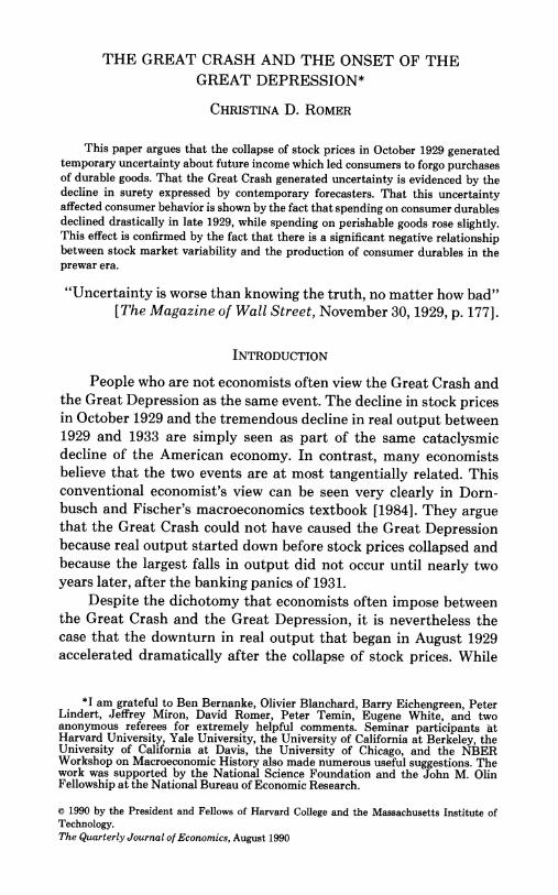
The Great Crash and the Onset of the Great DepressionAuthor(s): Christina D. RomerSource: The Quarterly Journal of Economics, Vol. 105, No. 3 (Aug., 1990), pp. 597-624Published by: The MIT PressStable URL: http://www.jstor.org/stable/2937892Accessed: 26/03/2010 00:27
Your use of the JSTOR archive indicates your acceptance of JSTOR's Terms and Conditions of Use, available athttp://www.jstor.org/page/info/about/policies/terms.jsp. JSTOR's Terms and Conditions of Use provides, in part, that unlessyou have obtained prior permission, you may not download an entire issue of a journal or multiple copies of articles, and youmay use content in the JSTOR archive only for your personal, non-commercial use.
Please contact the publisher regarding any further use of this work. Publisher contact information may be obtained athttp://www.jstor.org/action/showPublisher?publisherCode=mitpress.
Each copy of any part of a JSTOR transmission must contain the same copyright notice that appears on the screen or printedpage of such transmission.
JSTOR is a not-for-profit service that helps scholars, researchers, and students discover, use, and build upon a wide range ofcontent in a trusted digital archive. We use information technology and tools to increase productivity and facilitate new formsof scholarship. For more information about JSTOR, please contact [email protected].
The MIT Press is collaborating with JSTOR to digitize, preserve and extend access to The Quarterly Journal ofEconomics.
http://www.jstor.org
THE GREAT CRASH AND THE ONSET OF THE GREAT DEPRESSION*
CHRISTINA D. ROMER
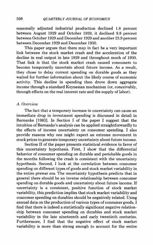
This paper argues that the collapse of stock prices in October 1929 generated temporary uncertainty about future income which led consumers to forgo purchases of durable goods. That the Great Crash generated uncertainty is evidenced by the decline in surety expressed by contemporary forecasters. That this uncertainty affected consumer behavior is shown by the fact that spending on consumer durables declined drastically in late 1929, while spending on perishable goods rose slightly. This effect is confirmed by the fact that there is a significant negative relationship between stock market variability and the production of consumer durables in the prewar era.
"Uncertainty is worse than knowing the truth, no matter how bad" [The Magazine of Wall Street, November 30, 1929, p. 177].
INTRODUCTION
People who are not economists often view the Great Crash and the Great Depression as the same event. The decline in stock prices in October 1929 and the tremendous decline in real output between 1929 and 1933 are simply seen as part of the same cataclysmic decline of the American economy. In contrast, many economists believe that the two events are at most tangentially related. This conventional economist's view can be seen very clearly in Dorn- busch and Fischer's macroeconomics textbook [1984]. They argue that the Great Crash could not have caused the Great Depression because real output started down before stock prices collapsed and because the largest falls in output did not occur until nearly two years later, after the banking panics of 1931.
Despite the dichotomy that economists often impose between the Great Crash and the Great Depression, it is nevertheless the case that the downturn in real output that began in August 1929 accelerated dramatically after the collapse of stock prices. While
*I am grateful to Ben Bernanke, Olivier Blanchard, Barry Eichengreen, Peter Lindert, Jeffrey Miron, David Romer, Peter Temin, Eugene White, and two anonymous referees for extremely helpful comments. Seminar participants at Harvard University, Yale University, the University of California at Berkeley, the University of California at Davis, the University of Chicago, and the NBER Workshop on Macroeconomic History also made numerous useful suggestions. The work was supported by the National Science Foundation and the John M. Olin Fellowship at the National Bureau of Economic Research.
? 1990 by the President and Fellows of Harvard College and the Massachusetts Institute of Technology. The Quarterly Journal of Economics, August 1990
598 QUARTERLY JOURNAL OF ECONOMICS
seasonally adjusted industrial production declined 1.8 percent between August 1929 and October 1929, it declined 9.8 percent between October 1929 and December 1929 and another 23.9 percent between December 1929 and December 1930.
This paper argues that there may in fact be a very important link between the stock market crash and the acceleration of the decline in real output in late 1929 and throughout much of 1930. That link is that the stock market crash caused consumers to become temporarily uncertain about future income. As a result, they chose to delay current spending on durable goods as they waited for further information about the likely course of economic activity. This decline in spending then drove down aggregate income through a standard Keynesian mechanism (or, conceivably, through effects on the real interest rate and the supply of labor).
A. Overview
The fact that a temporary increase in uncertainty can cause an immediate drop in investment spending is discussed in detail in Bernanke [1983]. In Section I of the paper I suggest that the intuition of Bernanke's analysis can be applied straightforwardly to the effects of income uncertainty on consumer spending. I also provide reasons why one might expect an extreme movement in stock prices to generate temporary uncertainty about future income.
Section II of the paper presents statistical evidence in favor of this uncertainty hypothesis. First, I show that the differential behavior of consumer spending on durable and perishable goods in the months following the crash is consistent with the uncertainty hypothesis. Second, I look at the correlation between consumer spending on different types of goods and stock market variability in the entire prewar era. The uncertainty hypothesis predicts that in general there should be an inverse relationship between consumer spending on durable goods and uncertainty about future income. If uncertainty is a consistent, positive function of stock market variability, this prediction implies that stock market variability and consumer spending on durables should be negatively related. Using annual data on the production of various types of consumer goods, I find that there is indeed a statistically significant negative relation- ship between consumer spending on durables and stock market variability in the late nineteenth and early twentieth centuries. Furthermore, I find that the negative effect of stock market variability is more than strong enough to account for the entire
THE GREAT CRASH AND THE GREAT DEPRESSION 599
decline in real consumer spending on durables that occurred in late 1929 and 1930.
While the statistical evidence is consistent with the notion that the Great Crash depressed consumption by generating uncertainty, it is important to supplement this evidence with direct information on whether uncertainty increased dramatically because of the stock market crash in late 1929. In Section III, I do this by examining the forecasts and analyses of five contemporary forecasters for the periods surrounding the recessions of 1921, 1924, and the stock market crash of 1929. This previously unexploited source provides a wealth of information about the expectations and uncertainty of sophisticated financial analysts in the 1920s. I find that forecasters were much more uncertain about the course of future income following the stock market crash than was typical even for unsettled times and that they specifically attributed this uncertainty to the Great Crash. I also find that these contemporary observers believed that consumer uncertainty was an important force depressing consumption.
Given that the uncertainty effects of the Great Crash of 1929 appear to explain the tremendous acceleration in the real economic decline that occurred in late 1929 and early 1930, it is natural to wonder why the collapse of stock prices in October 1987 was not followed by a similar depression. In Section IV of the paper I find that the relationship between stock price variability and consumer spending is quite similar in the prewar and postwar eras. At the same time I find that an important difference between the two crashes was that stock price variability in the year following the crash was much higher in 1929 than in 1987. These two facts are consistent with the view that the continued gyrations of stock prices in 1930 made consumers very nervous, while the comparatively smooth behavior of the stock market after the 1987 crash allowed consumers to view this crash as a one-time aberration. As a result, the 1987 crash did not depress spending to the extent that the 1929 crash did.
B. Competing Hypotheses
The explanation presented in this paper for the fall in real output in the year following the Great Crash is particularly useful because 1930 is arguably the most puzzling year of the Great Depression. While there are well-accepted monetary explanations for both the mild downturn in the summer of 1929 (see Hamilton [1987]) and for the severe collapse in late 1931 (see Friedman and
600 QUARTERLY JOURNAL OF ECONOMICS
Schwartz [1963]), Temin [1976] argues that the behavior of real and nominal interest rates suggests that monetary stringency could not be the main explanation for the real decline in 1930. This view has been echoed by others; Hamilton, for example, notes that the fact "that short term risk-free rates fell like a rock after 1929 reinforces the view that something besides high interest rates was leading the economy ever deeper into depression in 1930" [Hamilton, 1987, p. 1681.1 Temin's alternative explanation is that there was a decline in consumer spending in 1930 that cannot be accounted for simply by the fall in income. He bases this conclusion on the fact that consumer spending plummeted between 1929 and 1930, whereas it was reasonably steady in other significant interwar recessions.2
Several studies have tried to explain the decline in consumer spending noted by Temin. Not surprisingly, nearly all of these explanations have focused on the effects of the stock crash. One link that has been examined is the effect of the Great Crash on consumer expectations. It is possible that the crash depressed consumer spending simply by leading consumers to believe that the Great Depression was coming and hence that permanent income was lower. Temin [1976] examines the behavior of bond ratings and concludes from the fact that few bonds were downgraded following the crash that expectations did not turn decidedly negative in late 1929 or early 1930. This view that consumers did not suddenly become pessimistic is buttressed by Dominguez, Fair, and Shapiro [1988] who find that using data through 1929 and sophisticated statistical techniques, one would not predict a massive fall in real output in 1930.
A second link between the Great Crash and the drop in consumer spending that has been examined is the wealth effect of the decline in stock prices. It is possible that the crash depressed consumption simply by destroying a great deal of wealth. While this effect was no doubt present, Temin [1976] finds that the direct wealth effect of the stock price decline was fairly small. He bases this conclusion on the fact that stocks are a small fraction of total
1. According to Hamilton's figures, the yield on short-term government bonds fell from 4.80 percent in 1929 to 1.89 percent in 1930. The yield on long-term government bonds fell from 3.69 percent to 3.25 percent in the same period. Gordon and Wilcox [1982, pp. 70-74] also agree that a simple monetary explanation is inadequate for the first year of the Great Depression.
2. Mayer [1978a, 1978b] challenges Temin's evidence on the importance of consumption.

THE GREAT CRASH AND THE GREAT DEPRESSION 601
wealth and the fact that the estimated propensity to spend out of wealth in the interwar era is quite low.
Mishkin [1978] examines a third possible link between the Great Crash and the decline in consumption. He argues that the decline in financial assets caused by the crash, in conjunction with the rise in consumer liabilities resulting from the boom atmosphere of 1929, led to a deterioration in the household balance sheet. This decline in liquidity led consumers to fear for their solvency and thus to postpone the purchases of irreversible durable goods and hous- ing. Mishkin's evidence in favor of this hypothesis comes from equations estimated using postwar quarterly data. These regres- sions show a very strong impact of changes in the household balance sheet on consumer purchases of durables and new housing starts: the direct effect of the fall in financial assets and the rise in liabilities between 1929 and 1930 appears to account for two thirds of the observed drop in actual spending on these goods.
While the liquidity effect was surely operating in 1930, it is possible that the postwar coefficients that Mishkin uses overstate the effect of balance sheet changes in the interwar period, when durables were first being introduced and when consumers may have been more cautious about spending out of financial wealth. One piece of evidence that this is the case is that the model substantially overpredicts consumer spending on durables and housing earlier in the 1920s.3 This overprediction results from the fact that the postwar coefficient estimates predict a very strong positive effect from the tremendous rise in household financial assets that oc- curred between 1923 and 1929. That the prediction errors are quite large early in the 1920s suggests that the ability of Mishkin's model to explain the fall in consumption in 1930 should be viewed with caution.
This discussion of the evidence on possible links between the stock crash and the decline in real spending in late 1929 and all of 1930 suggests that none of the links analyzed so far is likely to
3. Using base data from Goldsmith, Lipsey, and Mendelson [1963] and adjust- ment and deflation procedures similar to those described in Mishkin [1978, Appencix, pp. 936-37], it is possible to extend Mishkin's balance sheet data back to 1923. Mishkin's coefficient estimates lead to the prediction that consumer expendi- tures on durable goods (in 1958 dollars) should have increased by $8.31 billion between 1923 and 1929 and real spending on residential housing should have risenby $5.40 billion. According to Kuznets' [1961] unpublished estimates of the components of GNP (converted to 1958 dollars), real consumer expenditures on durables rose only $3.65 billion and the value of gross nonfarm residential construction actually fell by $2.52 billion between 1923 and 1929.

602 QUARTERLY JOURNAL OF ECONOMICS
explain fully the acceleration of the real economic decline that began in this period. This suggests that an alternative explanation for the fall in consumer spending in late 1929 may indeed fill a gap in economists' understanding of the onset of the Great Depression.
I. THE UNCERTAINTY HYPOTHESIS
The uncertainty hypothesis investigated in this paper is very straightforward. I argue that the stock market crash of 1929 and the continued gyrations of stock prices throughout 1930 made people nervous about the future of the economy. That is, the extreme stock price variability of this period made people temporarily uncertain about the level of future income. This uncertainty in turn caused consumers to postpone purchases of irreversible durable goods.
A. Intuition
The intuition for why temporary uncertainty might depress consumer spending on durables is exactly analogous to that given in Bernanke [1983]. Consider a consumer deciding whether to buy a durable good that is available in varying levels of quality. When future income is temporarily uncertain and durables purchases are irreversible for long periods of time, there is a trade-off between purchasing the durable and waiting. If the consumer buys the durable, then he obviously gets the utility from the durable. However, the consumer is then locked into the durable before the level of future income is learned. Hence he may choose a quality level that is either too luxurious or too modest relative to his future income, and thus he may be very far from the optimal level of consumption for the life of the durable. On the other hand, if he waits, the consumer is very far from the optimal level of consump- tion while he is waiting, but he is then able to choose the appropriate durable good once the uncertainty about future income is resolved.
Given this trade-off, it is clear that a temporary rise in uncertainty will tend to increase the value of waiting. In such circumstances, consumers may find it advantageous to put off purchasing durables until they are more certain about the course of future income. A corollary to this finding that a temporary increase in income uncertainty may depress purchases of durable goods is that such a rise in uncertainty may stimulate purchases of nondura- bles. This occurs because consumers who are not buying durables will have more wealth available to spend on perishable (i.e., highly

THE GREAT CRASH AND THE GREAT DEPRESSION 603
reversible) goods. This differential behavior of durables and nondu- rables is an important feature that distinguishes the uncertainty hypothesis from more typical models of consumer behavior.4
While the preceding analysis of the effects of temporary income uncertainty has focused on consumers, it is clear that this story is also applicable to producers. For producers facing increasing re- turns, the relative payoff to various investment projects will clearly depend on the level of future income. If producers become tempo- rarily uncertain about future income, then it may be optimal for them to postpone purchases of new plant and equipment until they learn more about the future health of the economy. The effects of uncertainty on producers may in fact have been substantial in 1930. Indeed, such effects could explain why the output of producer durables fell substantially between 1929 and 1930 despite the drop in interest rates and the fairly optimistic forecasts of many business publications. I do not focus on the effect of uncertainty on producers, however, because the behavior of consumers has typi- cally been thought to be more important in this period.
B. Stock Market Variability and Uncertainty
While the intuition given above suggests that temporary income uncertainty could cause a drop in spending on durable goods, there remains the question of how and why an extreme movement in stock prices, such as the Great Crash of October 1929, might have generated widespread temporary uncertainty about future income. The fact that wild gyrations in stock prices cause the future income of stockholders to be more uncertain is one mecha- nism generating uncertainty. However, it cannot be the main mechanism by which such stock variability generates widespread income uncertainty because even in 1929 less than 2 percent of all American households held stock [Galbraith, 1988, p. 78].
A simple story about why extreme movements in stock prices cause uncertainty even among consumers who hold no stock starts from the premise that the stock market was thought to be an imperfect predictor of the real economy by consumers in the prewar economy. In this case, standard linear prediction theory indicates
4. Many other models predict that spending on durable goods will decline more than spending on nondurable goods because a larger movement in durables purchases is needed to yield a given change in the flow of durables services. However, these models do not predict that spending on nondurables will literally rise.
604 QUARTERLY JOURNAL OF ECONOMICS
that a larger than usual movement in stock prices will be associated with greater uncertainty about one's prediction of future income.
In the case of the Great Crash, there are more specific reasons to suspect that it generated extreme temporary uncertainty. One scenario that fits with many contemporary accounts is that people realized that the crash could disrupt credit markets and reduce investment. At the same time they were hopeful that the relatively new Federal Reserve System would step in and stabilize or stimu- late the economy. These contradictory possibilities following the Great Crash made people particularly uncertain about future income. Hence, both in general and in the particular case of 1929, it seems likely that extreme stock price movements did generate uncertainty about future income.
It is important to point out that this analysis of the effects of the Great Crash on consumer spending is partial equilibrium in two respects. First, it concerns consumer demand taking prices as given; that is, the analysis establishes that stock market variability can shift the aggregate demand curve back, but does not address the question of why a fall in aggregate demand does not simply lead to adjustment of prices. In the case of 1929-1930, the prices of consumer goods move surprisingly little despite large falls in real output. For example, the aggregate consumer price index fell less than 1 percent between October and December 1929 and less than 2 percent between January and June 1930. This stability of prices suggests that an explanation for the fall in aggregate demand in late 1929 is crucial for explaining the fall in real output in the first year of the Great Depression.
Second, the analysis does not take into account the fact that if people knew uncertainty tended to depress consumption, they should have been pessimistic following the Great Crash, not merely uncertain. This is true because a rational consumer would realize that if people became uncertain following the crash, they would cut their consumption and hence cause a decline in output for sure. The neglect of this possibility clearly rests on the assumption that prewar consumers did not know the true model of the economy.
II. STATISTICAL EVIDENCE
A. Behavior of Spending
The preceding discussion of the effects of uncertainty on consumption and the role of the stock market in generating
THE GREAT CRASH AND THE GREAT DEPRESSION 605
uncertainty suggests that one crucial prediction of the uncertainty hypothesis is that following the Great Crash there should have been a noticeable difference in the behavior of consumer spending on durable and perishable goods. Consumer spending on durable goods should have declined sharply following the collapse of stock prices, while spending on perishable goods should have actually risen.
There are two types of data that can be used to examine the behavior of consumer spending following the Great Crash. First, a variety of sources provide monthly data on retail sales of different types of consumer goods for the period around the Great Crash. The best known of the retail sales series is the Federal Reserve Board (FRB) index of department store sales. (The exact sources of this and all the other monthly spending series are given in the notes to Table I.) Department stores carry both durable consumer goods, such as furniture, floor coverings, and china, and semidurable consumer goods, such as clothing, shoes, and linens. Another available sales series that covers similar goods is the total value of sales from the two largest mail-order houses of this period, Montgom- ery Ward and Sears. A series that covers a purely durable good is new automobile registrations. Because of widespread registration, this series appears to provide a good measure of automobile sales.
There are two retail sales series that show the behavior of sales of nondurable goods. One is the value of sales of the four major five-and-ten-cent store chains. The other is the FRB index of the sales of grocery store chains. Since the FRB discontinued the grocery store sales series in January 1930 because it felt that the index was no longer representative of national grocery store sales, the quality of this series in the late 1920s is clearly somewhat suspect. Despite this flaw, it is useful to have these series on sales of nondurables to compare with the series on spending on durable goods.
Before these retail sales series can be used, it is necessary to make two adjustments. One is to convert them from nominal to real. This is accomplished by deflating using the consumer price index. The second is to adjust them for seasonal variation. This is done by regressing the percentage change of a given series on eleven monthly dummy variables and a constant.
In addition to these monthly retail sales data that are available only for the 1920s, there is an annual series that can be used as a proxy for the consumption of various types of goods for the entire prewar era. The Shaw [1947] series on real commodity output provides annual estimates of the output of durable, semidurable,
606 QUARTERLY JOURNAL OF ECONOMICS
and perishable goods destined for consumers, as well as a measure of total commodity output.5 The obvious flaw in this series is that it is an output series rather than a genuine consumption series. However, at least in the postwar era, the annual output of consumer goods and actual consumption are highly correlated. The main difference between the two series is that output is more cyclically sensitive because inventory investment is procyclical. Provided that the same relationships hold in the prewar era, the Shaw commodity output series should provide a reasonable (albeit excessively vola- tile) approximation for consumer expenditures.
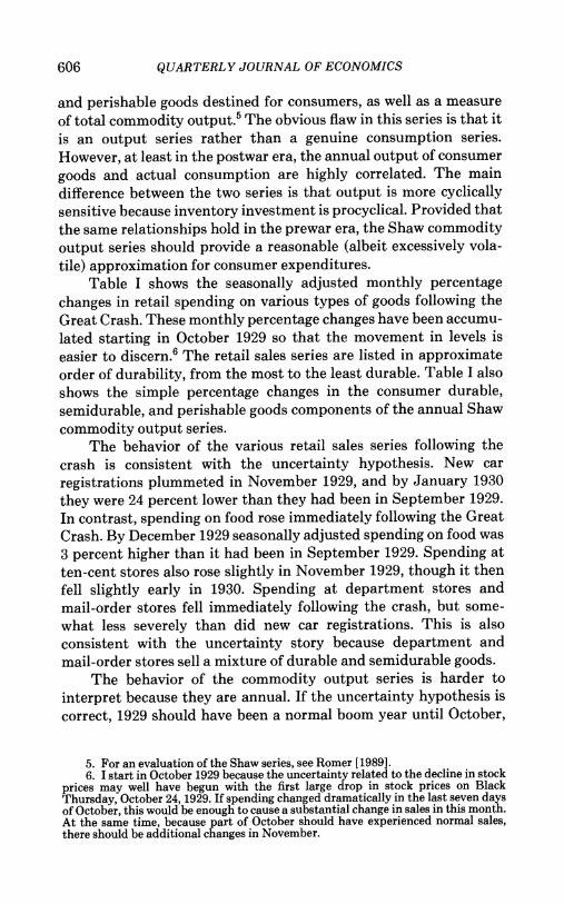
Table I shows the seasonally adjusted monthly percentage changes in retail spending on various types of goods following the Great Crash. These monthly percentage changes have been accumu- lated starting in October 1929 so that the movement in levels is easier to discern.6 The retail sales series are listed in approximate order of durability, from the most to the least durable. Table I also shows the simple percentage changes in the consumer durable, semidurable, and perishable goods components of the annual Shaw commodity output series.
The behavior of the various retail sales series following the crash is consistent with the uncertainty hypothesis. New car registrations plummeted in November 1929, and by January 1930 they were 24 percent lower than they had been in September 1929. In contrast, spending on food rose immediately following the Great Crash. By December 1929 seasonally adjusted spending on food was 3 percent higher than it had been in September 1929. Spending at ten-cent stores also rose slightly in November 1929, though it then fell slightly early in 1930. Spending at department stores and mail-order stores fell immediately following the crash, but some- what less severely than did new car registrations. This is also consistent with the uncertainty story because department and mail-order stores sell a mixture of durable and semidurable goods.
The behavior of the commodity output series is harder to interpret because they are annual. If the uncertainty hypothesis is correct, 1929 should have been a normal boom year until October,
5. For an evaluation of the Shaw series, see Romer [1989]. 6. I start in October 1929 because the uncertainty related to the decline in stock
prices may well have begun with the first large drop in stock prices on Black Thursday, October 24, 1929. If spending changed dramatically in the last seven days of October, this would be enough to cause a substantial change in sales in this month. At the same time, because part of October should have experienced normal sales, there should be additional changes in November.
THE GREAT CRASH AND THE GREAT DEPRESSION 607
TABLE I CONSUMER BEHAVIOR FOLLOWING THE GREAT CRASH
Cumulative percentage change in real seasonally adjusted retail sales
Oct. Nov. Dec. Jan. Feb. Mar. 1929 1929 1929 1930 1930 1930
Automobile registrations -5.5 -14.1 -18.9 -23.7 -11.7 -20.4 Department store sales -8.4 -10.1 -4.5 -15.8 -11.7 -16.4 Mail-order sales -4.1 -7.4 3.4 -20.6 -25.6 -35.8 Ten-cent store sales -0.3 1.7 -2.5 -2.7 -0.1 -7.4 Grocery store sales 5.9 3.1 3.4 NA NA NA
Percentage change in real output of consumer goods
1928 1929 1930
Durable goods 7.5 0.5 -32.4 Semidurable goods 4.1 1.8 -13.8 Perishable goods 1.6 4.3 -1.6
Sources. The series on new car registrations for 1925-1929 is from Standard Statistics Co., Standard Statistical Bulletin, 1930-31 Base Book, p. 182. The data for 1930 are from the Automobile Trade Journal and Motor Age. The department store sales series is from the Federal Reserve Bulletin, June 1944, p. 549. I use the version of the FRB index that covers the entire United States. The series on mail-order sales is from the Survey of Current Business, 1932 Annual Supplement, pp. 50-51, and various earlier issues. The series on ten-cent store sales is from the Standard Statistical Bulletin, 1932 Base Book, January 1932, p. 174. The series on grocery store sales is from the Federal Reserve Bulletin, April 1928, pp. 234-35, and later monthly issues of the Bulletin. The annual commodity output data are from Shaw [1947], Table I-3, pp. 70-77.
Notes: For all monthly series I use the version that has not already been adjusted for seasonal variation. The series for department stores sales, mail-order sales, and ten-cent store sales are deflated by the consumer price index for all goods, (CPI-W, 1957-59 = 100). The series for grocery store sales is deflated by the consumer price index for food (CPI-W, 1967 100). Both these price series are from the Bureau of Labor Statistics, Historical Summary from Detailed Monthly CPI Reports [19871. The deflated real retail sales series are seasonally adjusted by regressing the percentage changes of a given series on monthly dummy variables. The sample period used for this regression is 1919-1930 for all series except automobile registrations and grocery store sales for which only shorter samples are available. The Shaw series is expressed in 1913 prices.
and then consumer behavior should have changed greatly in the last two months. As a result, this change in behavior is likely to show part of its effect in 1929 and part in 1930. With this complication in mind, the commodity output data do appear to be consistent with the uncertainty hypothesis. The output of consumer durables, which had grown rapidly between 1927 and 1928, did not grow at all during 1929, and then fell sharply between 1929 and 1930. The output of perishables, on the other hand, grew much more rapidly in 1929 than it had in any other year in the 1920s. In 1930 this series eventually began to fall, but only slightly. Finally, the output of semidurables grew very slightly between 1928 and 1929 and then fell substantially between 1929 and 1930. As the uncertainty
608 QUARTERLY JOURNAL OF ECONOMICS
hypothesis would predict, the behavior of this class of goods was in-between that of durables and perishables (though somewhat closer to durables).
B. Consumer Spending and Stock Market Variability
While the behavior of various types of consumer spending following the Great Crash is clearly consistent with the uncertainty hypothesis, it is useful to present a more direct test of the uncertainty explanation for the onset of the Great Depression. This test is based on a second prediction of the uncertainty hypothesis: that, in general, extreme stock price variability should tend to depress consumer spending on durable goods and stimulate con- sumer spending on nondurable goods. These effects of stock price variability should be present regardless of whether the extreme movements are positive or negative, though the direct wealth effects of stock price movements will obviously depend on the sign of the change. If the uncertainty effects of the Great Crash are genuinely to explain the onset of the Great Depression, it should also be the case that the magnitude of the typical effect of stock variability is such that the estimated equation can predict the behavior of consumption in 1930.
While the quarterly, disaggregate consumption data that would be ideal for such a test do not exist before 1947, it is possible to use the Shaw commodity output series described above to examine consumer behavior starting in the late nineteenth century. To implement this test, I do the following. I regress the annual percentage change in the real output of a type of consumer good on its own lagged value, and on the lagged percentage change in total commodity output. These lagged values provide a very simple prediction model for the output of that class of good. To this simple prediction model I add a measure of the variability of real stock prices and the change in the real value of stock prices over the year. The variability measure is included as a proxy for the uncertainty generated by extreme movements in stock prices. The change in the level of real stock prices is included because movements in stock prices can obviously have a wealth effect as well as an uncertainty effect.
The equation that I estimate is
(1) Yit = ai + bjyjt-1 + ciyt-, + djVt + ejWt.
where yit and yt are the percentage changes in a category of commodity output and in total commodity output, respectively, Vt
THE GREAT CRASH AND THE GREAT DEPRESSION 609
is a measure of stock market variability, and Wt is the change in the level of real stock prices. The stock market variability measure that I include is simply the squared monthly change in real stock prices, averaged over a 12-month period.7 Because one would expect stock variability to have a rapid but not instantaneous effect on consumer behavior, I use the average of these squared changes from October of the preceding year to September of the given year to predict consumption in the given calendar year.8 Because wealth effects would probably also work with some delay, I lag the change in the level of real stock prices by one quarter as well.
This equation is estimated only over the period 1891-1928, so that the dramatic events of 1929 and 1930 cannot influence the results. I exclude the period of World War I and its aftermath (1914-1920) from the sample because the unusual events of this period might cause consumer behavior to be highly unusual and because the stock market was closed for several months following the outbreak of the war, making it impossible to compute a consistent variability measure.9
The resulting parameter estimates for equation (1) for the output of consumer durables, semidurables, and perishables are given in Table II. For the output of consumer durables, the estimated coefficient on the measure of stock market variability is negative and statistically significant. This indicates that both large positive and large negative movements in stock prices tend to depress the production of consumer durable goods just as the uncertainty hypothesis predicts. The coefficient is also very large. It implies that, holding everything else constant, doubling the variabil- ity measure from its average value of 0.001 depresses the annual output of consumer durables by nearly 7 percent.
7. The stock market index that I use is from Cowles [1939, Table P-1, pp. 66-67]. Because this is a nominal index, I deflate it by the Warren and Pearson wholesale price index for all commodities [1932, Table 1, pp. 6-10].
8. While the uncertainty hypothesis suggests that stock market variability and consumption should be related, it does not specify a particular lag structure for the relationship. In addition to the specification described above, I have tried several alternatives. Using the change in stock price variability rather than the level alters the coefficient estimates somewhat but does not change the qualitative results significantly. Including both the contemporaneous and lagged values of the stock market variability measure yields coefficients on V, that are nearly identical to those reported in Table II. Furthermore, this regression suggests that the lagged value of V, does not enter with the same, but opposite coefficient as the contemporaneous value.
9. If one creates a proxy for stock variability in 1914 (by averaging the squared changes of only the available monthly stock values) and then uses the full sample period 1891-1928, the estimation results do not change significantly.
610 QUARTERLY JOURNAL OF ECONOMICS
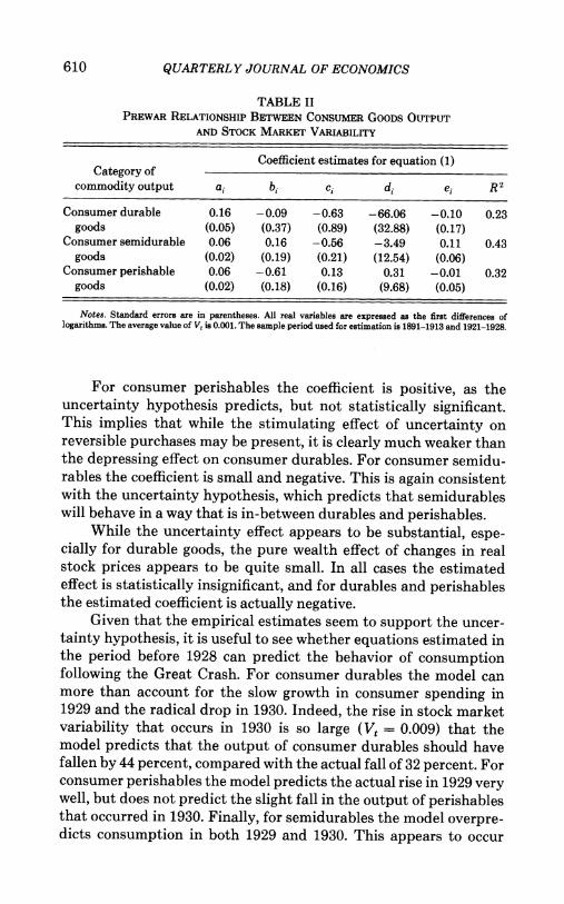
TABLE II PREWAR RELATIONSHIP BETWEEN CONSUMER GOODS OUTPUT
AND STOCK MARKET VARIABILITY
Coefficient estimates for equation (1) Category of
commodity output ai bi Ci di ei R 2
Consumer durable 0.16 -0.09 -0.63 -66.06 -0.10 0.23 goods (0.05) (0.37) (0.89) (32.88) (0.17)
Consumer semidurable 0.06 0.16 -0.56 -3.49 0.11 0.43 goods (0.02) (0.19) (0.21) (12.54) (0.06)
Consumer perishable 0.06 -0.61 0.13 0.31 -0.01 0.32 goods (0.02) (0.18) (0.16) (9.68) (0.05)
Notes. Standard errors are in parentheses. All real variables are expressed as the first differences of logarithms. The average value of Vt is 0.001. The sample period used for estimation is 1891-1913 and 1921-1928.
For consumer perishables the coefficient is positive, as the uncertainty hypothesis predicts, but not statistically significant. This implies that while the stimulating effect of uncertainty on reversible purchases may be present, it is clearly much weaker than the depressing effect on consumer durables. For consumer semidu- rables the coefficient is small and negative. This is again consistent with the uncertainty hypothesis, which predicts that semidurables will behave in a way that is in-between durables and perishables.
While the uncertainty effect appears to be substantial, espe- cially for durable goods, the pure wealth effect of changes in real stock prices appears to be quite small. In all cases the estimated effect is statistically insignificant, and for durables and perishables the estimated coefficient is actually negative.
Given that the empirical estimates seem to support the uncer- tainty hypothesis, it is useful to see whether equations estimated in the period before 1928 can predict the behavior of consumption following the Great Crash. For consumer durables the model can more than account for the slow growth in consumer spending in 1929 and the radical drop in 1930. Indeed, the rise in stock market variability that occurs in 1930 is so large (V, = 0.009) that the model predicts that the output of consumer durables should have fallen by 44 percent, compared with the actual fall of 32 percent. For consumer perishables the model predicts the actual rise in 1929 very well, but does not predict the slight fall in the output of perishables that occurred in 1930. Finally, for semidurables the model overpre- dicts consumption in both 1929 and 1930. This appears to occur
THE GREAT CRASH AND THE GREAT DEPRESSION 611
because semidurables behaved more like durables following the Great Crash than they typically did in the prewar era.
In sum, the statistical evidence is supportive of the uncertainty hypothesis. The behavior of various types of retail sales following the crash of 1929 fits the prediction of the uncertainty hypothesis that durables should decline greatly while more reversible pur- chases should decline much less, and in the case of perishable goods, should actually rise. The estimated correlation between consumer spending on various types of goods and stock market variability also supports the uncertainty hypothesis. In the prewar era, periods of high stock market variability tend to depress spending on durables, but stimulate (ever so slightly) spending on perishables.
III. QUALITATIVE EVIDENCE
In this section I investigate an entirely different type of evidence concerning the links between the crash of the stock market, uncertainty, and the fall in output in late 1929 and much of 1930. Specifically, I examine the forecasts and analyses of five contemporary business analysts over the 1920s to determine whether uncertainty was unusually high following the stock market crash, whether this uncertainty was caused by the crash, and whether uncertainty was believed to have an important negative effect on spending.
The particular forecasts that I analyze are those in Business Week, the Harvard Economic Society's Weekly Letters, The Maga- zine of Wall Street, Moody's Moody's Investors Service, and Standard Statistics Company's Standard Trade and Securities Service. These five business reports are representative of the many such magazines and forecasting services that provided economic information in the interwar period. These reports typically included a prediction about the behavior of output over the coming months and an analysis of the perceived cause of the current situation.
Because of their dual functions, these reports can provide two types of information about the importance of temporary uncer- tainty around the time of the Great Crash. First, since the forecast- ers typically provided some indication of their certainty about their predictions, the reports can show whether the forecasters them- selves became dramatically more uncertain about the course of economic activity following the collapse of stock prices in 1929 than they did during other periods of upheaval, such as 1920-1921. This kind of information is very helpful if one believes either that

612 QUARTERLY JOURNAL OF ECONOMICS
forecasters mirror the expectations of consumers or that forecasters play an important role in forming expectations.'0 Second, the analyses of the forecasters may indicate their impression of whether consumers were highly uncertain following the crash and whether this was a major factor depressing consumer spending.
A. Forecaster Uncertainty
The information that the forecasts provide about forecaster uncertainty due to the Great Crash is striking. An analysis of the confidence expressed by the forecasters shows that forecasters became uncertain immediately following the Great Crash to an extent that was unprecedented in the 1920s. Furthermore, this uncertainty, while perhaps resolved somewhat in the spring of 1930, appears to resurface by mid-1930.
1929. Among the five forecasters, four became definitely more uncertain about the future of business immediately following the collapse of stock prices in late October 1929. Moreover, the forecast- ers who became less confident indicated that it was because of the stock market crash. This change is particularly noticeable in the Harvard Economic Society's Weekly Letters (referred to as Har- vard in the following discussion). In early October 1929 Harvard was certain that a mild downturn was in store for the economy. It stated: "business is thus facing another period of readjustment" [October 19, 1929, p. 252]. Following the crash, however, Harvard became very uncertain. It said: "the unprecedented declines in stock prices ... make it difficult to estimate at present the amount of injury which will be done to business" [November 16, 1929, p. 274]. Furthermore, Harvard specifically mentioned that it felt that this uncertainty was temporary and that "a month hence it may be possible to appraise the situation more satisfactorily and present a definite forecast for the year 1930" [November 16, 1929, p. 276].
This same pattern is also shown in Moody's Investors Service (Moody's), Standard Trade and Securities Service (Standard), and Business Week. While all three of these forecasters appear to have been very certain of their forecasts in the late summer of 1929, they were decidedly uncertain following the Great Crash. In mid-November Moody's stated: "the extent of net paper losses and their effect can hardly be measured for the country as a whole" [November 18, 1929, p. I-241]. A week later Standard wrote that the
10. Gramlich [1983] suggests that in some situations the forecasts of profes- sional forecasters provide a reasonably good proxy for consumer expectations.
THE GREAT CRASH AND THE GREAT DEPRESSION 613
"full significance of the drastic drop in security values on future business can in no wise be measured" [November 27, 1929, p. 1]. Finally, Business Week said at the start of 1930: "the forecasters cannot yet read the riddle of 1930" [January 8, 1930, p. 48].
In contrast to the other forecasters, The Magazine of Wall Street (Wall Street) appears to have been nearly as certain of its forecasts after the crash as it was before the crash. For example, in November 1929 it stated with confidence that "the general outlook for trade and industry is thus one in which moderate restraint may be evidenced for some months, but ... recovery to a fair measure of prosperous conditions may be anticipated before the new year is far advanced" [November 16, 1929, p. 96].
In addition to the fact that all the forecasters except one expressed less confidence in their forecasts, there was also more divergence than usual in the point estimates of the forecasts shortly after the Great Crash. Evidence that this was the case is provided by the fact that the forecasters themselves commented frequently on this divergence. Standard noted that "with the opening of the new year, there is a wide conflict of opinion as to what is in store for industry and commerce during the early part of 1930" [January 3, 1930, p. 1]. Business Week also noted that "opinions may differ as to whether or not the stock market collapse ... need necessarily be followed by a serious business recession" [November 30, 1929, p. 44]. Such divergence of opinion may have been important if one believes that forecasters do not merely mirror public expectations, but actually affect them. In late 1929 consumers and producers may have been made quite uncertain by the conflicting predictions they were receiving from the economic experts.
1920s. While this evidence suggests that forecaster uncertainty increased following the Great Crash of October 1929, it does not indicate whether this was an unusual event. It could be that forecasters always became uncertain in downturns. To get a sense of whether the rise in uncertainty in November 1929 was unusual, I analyze the forecasts of the same forecasters examined above for the periods surrounding the recessions of 1920-1921 and 1923-1924."
This analysis shows that the dramatic change in forecasters' expressions of confidence that followed the Great Crash did not
11. No forecasts are analyzed for Business Week for these earlier cycles because the magazine only came into existence in August 1929. For 1920-1921, the material which later appears in Harvard's Weekly Letters is contained in the Review of Economic Statistics [1920-1921]. For 1920-1924, Moody's forecasts are published in Moody's Investment Letters [1920-1924].
614 QUARTERLY JOURNAL OF ECONOMICS
occur in either 1921 or 1924. In these earlier downturns there was never a time when several of the forecasters simultaneously ex- pressed greater uncertainty. Furthermore, many of the forecasters were equally confident throughout both 1921 and 1924. For exam- ple, Harvard stated with surety in February 1924 that "conditions thus remain favorable to the maintenance of generally good busi- ness conditions" [February 2, 1924, p. 28] and again in May 1924 with equal confidence that "business is not now facing a period of general depression" [May 17, 1924, p. 134].
In the 1920s some of the forecasters did periodically express uncertainty about their forecasts, but these statements seem to be vague disclaimers, the essence of which is that forecasting is difficult. For example, Standard frequently included such state- ments as "the view itself is to be interpreted as an estimate of the probabilities, rather than as a cocksure forecast" [November 26, 1923, p. 375]. There does not appear to be any systematic pattern to these disclaimers, and they occurred at radically different times for different forecasters. Furthermore, they were never followed by statements about when the forecaster expected to be more certain as they often are in 1929. Thus, this analysis suggests that the tremendous rise in temporary uncertainty shown by forecasters in 1929 was indeed an unusual event.
1930. While it appears that the rise in uncertainty due to the stock market crash in late 1929 and early 1930 can explain why output plummeted immediately following the crash, there remains the question of why the economy remained depressed and in fact continued to decline through all of 1930. Judging from the five business analyses that I have examined, the answer may be that uncertainty continued or at least reappeared at various points in 1930.
Standard appears to have remained highly uncertain through much of 1930. In March, for example, it wrote that "uncertainties in the situation are still too numerous to permit the formation of an iron-bound opinion as regards the longer term prospect for indus- trial production" [March 19, 1930, p. 1]. Many other forecasters, however, appear to have become both very positive and very certain in the spring of 1930. For example, Moody's stated in April that "the inescapable conclusion is that we are not facing a business depression" [April 24, 1930, p. 1-172]. Similarly, Harvard, which had said in November that it could not make a forecast, stated in
THE GREAT CRASH AND THE GREAT DEPRESSION 615
April that "what this forecast means for second quarter business may now be indicated more precisely" [April 19, 1930, p. 104].
The apparent certainty of these forecasters may indicate that some of the uncertainty related to the Great Crash was resolved in the spring of 1930. But it is also possible that this confidence should not be taken at face value. Hoover's main response to the stock market crash and the ensuing decline in real output was to promulgate optimistic forecasts and to encourage others to do so as well. According to Standard, "officialdom takes the attitude that its function is to point out whatever is bright in the picture" [March 19, 1930, p. 3]. It is possible that the professional analysts participated in this prosperity propaganda program and introduced into their forecasts a degree of manufactured optimism. Standard clearly felt this was the case when it stated in the spring of 1930 that, "the tendency of the press is to pick out and play up those features which are hopeful and either to omit or to play down those features which are not so good" [May 28, 1930, p. 2].
In addition to the fact that some of the forecasters may have been artificially certain in early 1930, most of the forecasters were openly uncertain again in the summer. For example, Moody's seemed to be quite unsure of its current forecast when it stated in June that "within the next two or three months it may be possible to say with more certainty just how far this improvement will go and whether it will be sustained or not" [June 27, 1930, p. 1-280]. Business Week suggested that it was the continued gyrations of stock prices that made it unsure of its forecasts in 1930. It stated: "if the stock market can similarly adjust itself to realities without smashing anything in the next month ..., we should be able to settle down to a fairly respectable domestic life this summer" [April 19, 1930, p. 5].
B. Consumer Uncertainty
As mentioned above, the forecasts of the five business analysts not only provide evidence of their own expectations, but also their analyses of the determinants of consumer behavior. While these analyses are clearly not based on widespread surveys of consumer sentiment, it is nevertheless useful to see whether the uncertainty story told in this paper struck contemporary analysts as plausible.
1929. Before the 1929 crash, most of the analysts barely mentioned consumers. Those that did merely stressed that consump- tion was at record levels. For example, Moody's stated in August
616 QUARTERLY JOURNAL OF ECONOMICS
1929 that "the large purchasing power in the hands of the people will keep on transmuting itself into effective retail demand for all kinds of consumption goods" [August 12, 1929, p. I-174].
After the crash every one of the forecasters stressed that consumers were very uncertain about the future of the economy. Moody's, for example, argued that the factors which "may ulti- mately prove more important than any calculated estimate of losses in purchasing power ... [are] the individual attitude and sentiment of people who have been affected by the stock market" [November 18, 1929, p. 1-242]. In December Moody's was even more explicit about the rise in uncertainty. It discussed "the stock market break, which undermined general confidence" and indicated that "during the past few weeks almost everybody held his plans in abeyance and waited for the horizon to clear" [December 16, 1929, p. 1-257].
Standard, like Moody's, not only mentioned the rise in uncer- tainty, but also differentiated its effect on consumer spending from the effect of the decline in wealth. Several issues of its report in the fall of 1929 contained statements such as: "reflecting the loss of purchasing power, as well as public confidence, resulting from the collapse of security values, we anticipate a sizable decline in internal business during early future months" [November 20, 1929, p. 1]. Harvard, while not discussing consumer uncertainty directly, noted that "coinciding with the break in stock prices, department store trade showed a pronounced shrinkage" [November 30, 1929, p. 284] and referred to "a spirit of caution widely prevalent" [Decem- ber 21, 1929, p. 308].
Business Week and The Magazine of Wall Street also believed that consumers became very uncertain following the stock market crash. In early November Business Week referred to "the hysteria that accompanied the market upheaval" and the resulting "suspi- cious and nervous public" [November 2, 1929, p. 3]. Wall Street emphasized the mechanism by which uncertainty affects the econ- omy when it stated that "in itself, a severe reaction in stock prices has an unfavorable influence on general trade both by curtailing purchasing power and by impairing the confidence of consumers and businessmen alike." It also noted that as a result of this uncertainty, "there has been a tendency to reduce or postpone projected commitments" [both quotations, November 16, 1929, p. 94].
1930. The analysis that the forecasters gave of consumer confidence also suggests that the unusual level of uncertainty in late 1929 continued and perhaps increased through 1930 and that this

THE GREAT CRASH AND THE GREAT DEPRESSION 617
continued uncertainty may explain the continued decline in real output. Moody's, for example, stated that "the recent conservatism in buying [is] caused by lower purchasing power and accentuated by psychological uncertainties" [July 24, 1930, pp. I-303-04]. Stan- dard spoke of "this particular time of persistent uncertainty throughout the country" [April 23, 1930, p. 2], and Business Week stated that "there is a widespread and disquieting uncertainty as to how far this recovery will go and how long it will be before normal levels of activity will again be approached" [February 22, 1930, back cover].
Continued stock price declines were thought to have been a major factor making consumers nervous. Harvard, for example, after discussing at length the "sharp fluctuations in the stock market," stated in May 1930 that "doubtless this continued hesi- tancy [of spending] may be attributed partly to the drop in stock prices" [May 17, 1930, p. 125 and p. 126, respectively]. Again in June Harvard wrote: "the repeated severe reactions in stock prices are important factors holding back business revival because of their wide effect upon sentiment" [June 21, 1930, p. 155]. A similar view was expressed by Wall Street. It suggested that because "the sharp first quarter rally witnessed in the stock market terminated promptly when the underpinning of business facts was found inadequate to warrant such false hopes," "uncertainty and confused price trends have been the new order of the day" [both quotations, June 14, 1930, p. 254].
While continued stock price movements were a major factor thought to be generating consumer uncertainty, other factors were also assigned some blame. Business Week suggested that "business is now suffering chiefly from a pain in the expectations, due mainly to the overproduction of official forecasts of early and easy return of the swell times of yesteryear" [May 14, 1930, p. 1]. It seems quite possible that Hoover's prosperity propaganda program contributed to the uncertainty of consumers in 1930 by generating forecasts that were so at odds with actual economic conditions. Other factors that were mentioned as a source of uncertainty in early 1930 were the "suspense and indecision created by the final outcome of the new rates included in the Hawley-Smoot tariff bill" [Wall Street, June 14, 1930, p. 289] and "alarm about the continuing weakness in prominent commodity markets" [Harvard, June 21, 1930, p. 1541.
This evidence indicates that the five business analysts all viewed consumers as being unusually uncertain in 1929 because of the stock market crash and remaining uncertain throughout much
618 QUARTERLY JOURNAL OF ECONOMICS
of 1930.12 While there is not universal agreement on the source of this continued uncertainty, its presence can explain why consumer spending failed to recover, and in fact declined further, during 1930.
IV. COMPARISON OF 1987 AND 1929
This paper has investigated a possible link between the stock market crash of October 1929 and the rapid acceleration of real economic decline in late 1929 and all of 1930. The paper has used economic analysis, statistical results, and qualitative evidence on expectations to suggest that the Great Crash temporarily increased uncertainty about the course of future income and that this uncertainty caused consumers to cut spending on durable goods drastically. This story resolves an important puzzle about the onset of the Great Depression: it explains why consumer spending dropped precipitously in late 1929 and early 1930 despite the fact that monetary policy was quite loose and expectations were reason- ably sanguine.
Given the finding of a link between the Great Crash and the onset of the Great Depression, it is natural to consider the relevance of this analysis to the stock market crash of 1987. Between September and October 1987 real stock prices fell 13 percent. This is in fact larger than the 10 percent drop in real stock prices that occurred between September and October 1929. If the story told in this paper is correct, one might expect a significant fall in consump- tion to have occurred in late 1987 just as it did in 1929.
To some degree this is the case. Total consumer spending (in 1982 dollars) fell at a seasonally adjusted annual rate of 2.1 percent between the third and fourth quarters of 1987. A fall of this magnitude had previously only occurred in severe recession years, such as 1958 or 1974. The composition of this fall was also consistent with the uncertainty hypothesis. Consumer spending on durable goods fell at an annual rate of 19 percent between the third and fourth quarters of 1987, with automobiles being particularly hard hit. Total spending on nondurable goods essentially did not change at all, and several components actually rose. The only nondurable spending category that fell substantially was cloth-
12. This emphasis on consumer uncertainty in 1929-1930, like the forecasters' own expressions of uncertainty, did not occur in earlier recessions. Consumer behavior was rarely mentioned in the forecasters' analysis of 1920-1921 and 1923-1924, and in no instance did the forecasters indicate that consumer spending was being affected by uncertainty.
THE GREAT CRASH AND THE GREAT DEPRESSION 619
ing-a category that is more appropriately classified as semidurable and that may therefore be somewhat depressed by uncertainty. Finally, spending on services rose at a robust annual rate of 2.2 percent.
While consumption behaved as the uncertainty hypothesis would predict in the fourth quarter of 1987, the effect was substan- tially shorter lived in 1987 than in 1929. Whereas the fall in consumer spending that started in late 1929 intensified throughout 1930, the drop in consumption following the crash of 1987 reversed itself in the first quarter of 1988. Between the fourth quarter of 1987 and the first quarter of 1988 total consumer spending rose at an annual rate of 4.4 percent and spending on durables rose at an annual rate of 13.7 percent.
A. Statistical Evidence
An examination of the postwar relationship between consump- tion and stock market variability provides some explanation for the differences in consumer behavior between 1929 and 1987. It is possible to run the regressions specified in equation (1) for the period 1949-1986. To preserve the comparability of the prewar and postwar regressions, I use the annual output of various classes of consumer goods as the dependent variable.'3 The results of these regressions are given in Table III.
For the most part the postwar results are remarkably similar to those for the prewar era.'4 In the postwar era, periods of extreme stock market variability are highly correlated with drops in the production of consumer durables. According to the estimates, a doubling of the stock variability measure from its average value of 0.001 reduces the annual output of consumer durables by 6.2 percent. This effect is highly statistically significant and only slightly smaller than the prewar effect, which was a drop in the annual output of durables of 6.6 percent for a similar change in
13. The exact series that I use are the Federal Reserve Board annual indexes of the output of final consumer durable and nondurable goods. The FRB index of total final products (plus intermediate construction supplies) is used as the equivalent of the Shaw measure of total commodity output. The real stock price series is created by deflating the Standard and Poor Composite Stock Price Index (for 500 stocks) by the producer price index for all commodities. All postwar data are from the Citibase databank (January 1989 version).
14. As with the prewar equations, it is possible to try alternative specifications for the relationship between stock market variability and the output of consumer goods. Including a lagged value of Vt does not alter the coefficient on the contemporaneous value of variability appreciably. However, this specification does suggest some lagged effects of stock market variability.
620 QUARTERLY JOURNAL OF ECONOMICS
TABLE III POSTWAR RELATIONSHIP BETWEEN CONSUMER GOODS OUTPUT
AND STOCK MARKET VARLkBiLrTY
Coefficient estimates for equation (1) Category of
commodity output ai bi ci di ei R 2
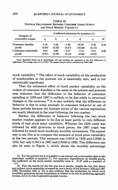
Consumer durable 0.18 0.29 -1.90 -62.05 -0.20 0.44 goods (0.04) (0.20) (0.47) (19.29) (0.10)
Consumer nondurable 0.03 0.69 -0.37 -5.74 0.01 0.36 goods (0.01) (0.29) (0.12) (4.92) (0.02)
Notes. Standard errors are in parentheses. All real variables are expressed as the first differences of logarithms. The average value of Vt is 0.001. The sample period used for estimation is 1949-1986.
stock variability.'5 The effect of stock variability on the production of nondurables in the postwar era is essentially zero, and is not statistically significant.
That the estimated effect of stock market variability on the output of consumer durables is the same in the prewar and postwar eras indicates that the difference in the behavior of consumer spending in 1929 and 1987 is unlikely to be due solely to structural changes in the economy.'6 It is also unlikely that the difference in behavior is due to some anomaly in consumer behavior in one of these periods because the forecast errors of the various regressions are nearly identical in the year following the two crashes.
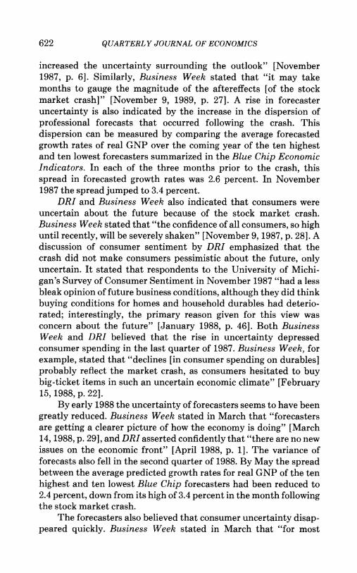
Rather, the difference in behavior following the two stock market crashes appears to be due at least partly to very different levels of real stock price variability. Whereas the 1929 crash was followed by wild gyrations in stock prices, the 1987 crash was followed by much more moderate monthly movements. The easiest way to see this is to compare the measure of stock price variability in the two periods. This measure was 0.0019 in 1929 and 0.0090 in 1930, but only 0.0013 in 1987 and 0.0036 in 1988. This difference can also be seen in Figure I, which shows the monthly percentage
15. For the postwar era it is possible to use annual real consumption data as the dependent variable in equation (1). For consumer expenditures on durable goods, the coefficient on the stock market variability term is -31.97 with a t-statistic of -2.3.
16. That the results for the two eras are so similar, despite the fact that direct and indirect stock ownership increased by over a factor of ten between 1929 and 1987 [DRI, November 1987, p. 151, is also evidence that the mechanism by which stock variability generates income uncertainty is related to its role in predicting aggregate income, not to its role in generations asset income.
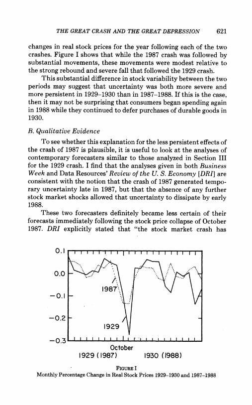
THE GREAT CRASH AND THE GREAT DEPRESSION 621
changes in real stock prices for the year following each of the two crashes. Figure I shows that while the 1987 crash was followed by substantial movements, these movements were modest relative to the strong rebound and severe fall that followed the 1929 crash.
This substantial difference in stock variability between the two periods may suggest that uncertainty was both more severe and more persistent in 1929-1930 than in 1987-1988. If this is the case, then it may not be surprising that consumers began spending again in 1988 while they continued to defer purchases of durable goods in 1930.
B. Qualitative Evidence
To see whether this explanation for the less persistent effects of the crash of 1987 is plausible, it is useful to look at the analyses of contemporary forecasters similar to those analyzed in Section III for the 1929 crash. I find that the analyses given in both Business Week and Data Resources' Review of the U. S. Economy [DRI] are consistent with the notion that the crash of 1987 generated tempo- rary uncertainty late in 1987, but that the absence of any further stock market shocks allowed that uncertainty to dissipate by early 1988.
These two forecasters definitely became less certain of their forecasts immediately following the stock price collapse of October 1987. DRI explicitly stated that "the stock market crash has
0 .1 I , , , , I , I I I I I I I I I I I I
0.0
-0.1187
-0.2 / 1929
- 0 .3 A I I I I I I I I I . .
October 1929 (1987) 1930 (1988)
FIGURE I Monthly Percentage Change in Real Stock Prices 1929-1930 and 1987-1988
622 QUARTERLY JOURNAL OF ECONOMICS
increased the uncertainty surrounding the outlook" [November 1987, p. 6]. Similarly, Business Week stated that "it may take months to gauge the magnitude of the aftereffects [of the stock market crash]" [November 9, 1989, p. 27]. A rise in forecaster uncertainty is also indicated by the increase in the dispersion of professional forecasts that occurred following the crash. This dispersion can be measured by comparing the average forecasted growth rates of real GNP over the coming year of the ten highest and ten lowest forecasters summarized in the Blue Chip Economic Indicators. In each of the three months prior to the crash, this spread in forecasted growth rates was 2.6 percent. In November 1987 the spread jumped to 3.4 percent.
DRI and Business Week also indicated that consumers were uncertain about the future because of the stock market crash. Business Week stated that "the confidence of all consumers, so high until recently, will be severely shaken" [November 9, 1987, p. 28]. A discussion of consumer sentiment by DRI emphasized that the crash did not make consumers pessimistic about the future, only uncertain. It stated that respondents to the University of Michi- gan's Survey of Consumer Sentiment in November 1987 "had a less bleak opinion of future business conditions, although they did think buying conditions for homes and household durables had deterio- rated; interestingly, the primary reason given for this view was concern about the future" [January 1988, p. 46]. Both Business Week and DRI believed that the rise in uncertainty depressed consumer spending in the last quarter of 1987. Business Week, for example, stated that "declines [in consumer spending on durables] probably reflect the market crash, as consumers hesitated to buy big-ticket items in such an uncertain economic climate" [February 15, 1988, p. 22].
By early 1988 the uncertainty of forecasters seems to have been greatly reduced. Business Week stated in March that "forecasters are getting a clearer picture of how the economy is doing" [March 14, 1988, p. 29], and DRI asserted confidently that "there are no new issues on the economic front" [April 1988, p. 1]. The variance of forecasts also fell in the second quarter of 1988. By May the spread between the average predicted growth rates for real GNP of the ten highest and ten lowest Blue Chip forecasters had been reduced to 2.4 percent, down from its high of 3.4 percent in the month following the stock market crash.
The forecasters also believed that consumer uncertainty disap- peared quickly. Business Week stated in March that "for most
THE GREAT CRASH AND THE GREAT DEPRESSION 623
consumers, the stock market crash is just a fading memory" [March 21, 1988, p. 42]. DRI stated in the same month that "consumers have regained much of their confidence" [March 1988, p. 52]. The forecasters' statements soon after the crash suggest that the absence of further stock price movements may have been an important factor leading to this reduction in uncertainty. Business Week stated in late November: "so much rests on the stock market's performance in the weeks ahead. If it rises-or even if it gets no worse-consumer spending is not likely to suffer enough to place the five-year economic advance in jeopardy" [November 23, 1988, p. 27]. Similarly, DRI stated that "one risk to this forecast is the volatility of the stock market. If extreme movements continue, consumer confidence may be weakened more than projected" [November 1987, p. 55]. DRI echoed this view that stock stability was crucial to the health of the economy seven months later. It stated "although the economy survived that crash very nicely, it is unclear that it could survive a repeat without a substantial recession" [June 1988, p. 5].
This qualitative evidence, along with the empirical results, suggests that continued stock price movements prolonged uncer- tainty in 1929 in a way that they did not in 1987. Whether this was the crucial difference between 1930 and 1988 is hard to say. Certainly, other factors, such as the basic health of the economy and economic policy, also differed in the two periods. Nevertheless, the analysis of this paper suggests that uncertainty is a potent determi- nant of consumer behavior and thus the differences in the level of uncertainty in the two periods could explain why the crash of 1929 was followed by the Great Depression and the crash of 1987 was not.
UNIVERSITY OF CALIFORNIA, BERKELEY, AND
NATIONAL BUREAU OF ECONOMIC RESEARCH
REFERENCES
Automobile Trade Journal and Motor Age, 1930. Bernanke, Ben S., "Irreversibility, Uncertainty, and Cyclical Investment," Quar-
terly Journal of Economics, XCVIII (1983), 85-106. Blue Chip Economic Indicators, 1987-1988. Business Week, 1929-1930,1987-1988. Cowles, Alfred, and Associates, Common-Stock Indexes, 2nd ed. (Bloomington, IN:
Principia Press, 1939). Data Resources, Inc., Review of the U. S. Economy, 1987-1988. Dominguez, Kathryn M., Ray C. Fair, and Matthew D, Shapiro, "Forecasting the
Depression: Harvard versus Yale," American Economic Review, LXXVIII (1988), 595-612.
Dornbusch, Rudiger, and Stanley Fischer, Macroeconomics, 3rd ed. (New York: McGraw Hill, 1984).
624 QUARTERLY JOURNAL OF ECONOMICS
Friedman, Milton, and Anna J. Schwartz, A Monetary History of the United States, 1867-1960 (Princeton, NJ: Princeton University Press for NBER, 1963).
Galbraith, John Kenneth, The Great Crash 1929 (Boston: Houghton Mifflin, 1988). Goldsmith, Raymond W., R. E. Lipsey, and M. Mendelson, Studies in the National
Balance Sheet of the United States (Princeton, NJ: Princeton University Press, 1963).
Gordon, Robert J., and James A. Wilcox, "Monetarist Interpretations of the Great Depression: An Evaluation and Critique," in The Great Depression Revisited, Karl Brunner, ed. (Boston: Martinus Nijhoff, 1981).
Gramlich, Edward M., "Models of Inflation Expectations Formation," Journal of Money, Credit and Banking, XV (1983), 155-173.
Hamilton, James D., "Monetary Factors in the Great Depression," Journal of Monetary Economics, XIX (1987), 145-69.
Harvard Economic Society (or Service), Weekly Letters, 1923-1930. Kuznets, Simon S., unpublished technical tables underlying Capital in the Ameri-
can Economy: Its Formation and Financing (Princeton, NJ: Princeton Univer- sity Press for NBER, 1961).
The Magazine of Wall Street, 1920-1930. Mayer, Thomas, "Consumption in the Great Depression," Journal of Political
Economy, LXXXVI (1978a), 139-45. , "Money and the Great Depression: A Critique of Professor Temin's Thesis," Explorations in Economic History, XV (1978b), 127-45.
Mishkin, Frederic S., "The Household Balance Sheet and the Great Depression," Journal of Economic History, XXXVII (1978), 918-37.
Moody's Investors Service, Moody's Investors Service (Business and Industry Guide), 1929-1930. ,Moody's Investment Letters, 1920-1924.
Review of Economic Statistics, 1920-1921. Romer, Christina D., "The Prewar Business Cycle Reconsidered: New Estimates of
Gross National Product, 1869-1908," Journal of Political Economy, XCVII (1989), 1-37.
Shaw, William H., Value of Commodity Output since 1869 (New York: NBER, 1947).
Standard Statistics Co., Standard Daily Trade Service, 1920-1924. ,Standard Statistical Bulletin, 1920-1931 and 1932 Base Books. ,Standard Trade and Securities Service (General Section), 1929-1930.
Temin, Peter, Did Monetary Forces Cause the Great Depression? (New York: W. W. Norton, 1976).
Warren, G. F., and F. A. Pearson, Wholesale Prices in the United States for 135 Years, 1797-1932, Cornell University Agricultural Experiment Station Memoir 142, November 1932.
U. S. Board of Governors of the Federal Reserve System, Federal Reserve Bulletin, 1928-1944.
U. S. Bureau of Foreign and Domestic Commerce, Survey of Current Business, 1922-1932.
U. S. Bureau of Labor Statistics, Historical Summary from Detailed Monthly CPI Reports, microfiche, 1987.