Embed Size (px)
Citation preview
The Astrophysical Journal, 767:65 (23pp), 2013 April 10 doi:10.1088/0004-637X/767/1/65C© 2013. The American Astronomical Society. All rights reserved. Printed in the U.S.A.
THE HABITABLE ZONE OF EARTH-LIKE PLANETS WITH DIFFERENT LEVELSOF ATMOSPHERIC PRESSURE
Giovanni Vladilo1,2, Giuseppe Murante1, Laura Silva1, Antonello Provenzale3,Gaia Ferri2, and Gregorio Ragazzini2
1 INAF-Trieste Astronomical Observatory, Trieste, Italy; [email protected] Department of Physics, University of Trieste, Trieste, Italy
3 Institute of Atmospheric Sciences and Climate-CNR, Torino, ItalyReceived 2012 December 14; accepted 2013 February 15; published 2013 March 25
ABSTRACT
As a contribution to the study of the habitability of extrasolar planets, we implemented a one-dimensional energybalance model (EBM), the simplest seasonal model of planetary climate, with new prescriptions for most physicalquantities. Here we apply our EBM to investigate the surface habitability of planets with an Earth-like atmosphericcomposition but different levels of surface pressure. The habitability, defined as the mean fraction of the planet’ssurface on which liquid water could exist, is estimated from the pressure-dependent liquid water temperature range,taking into account seasonal and latitudinal variations of surface temperature. By running several thousands ofEBM simulations we generated a map of the habitable zone (HZ) in the plane of the orbital semi-major axis, a,and surface pressure, p, for planets in circular orbits around a Sun-like star. As pressure increases, the HZ becomesbroader, with an increase of 0.25 AU in its radial extent from p = 1/3 to 3 bar. At low pressure, the habitability is lowand varies with a; at high pressure, the habitability is high and relatively constant inside the HZ. We interpret theseresults in terms of the pressure dependence of the greenhouse effect, the efficiency of horizontal heat transport, andthe extent of the liquid water temperature range. Within the limits discussed in the paper, the results can be extendedto planets in eccentric orbits around non-solar-type stars. The main characteristics of the pressure-dependent HZare modestly affected by variations of planetary properties, particularly at high pressure.
Key words: astrobiology – planetary systems
Online-only material: color figures
1. INTRODUCTION
Observational searches for extrasolar planets are motivated,in large part, by the quest for astronomical environments withphysical and chemical conditions supportive of life. The crite-rion most commonly adopted to define such “habitable” environ-ments is the presence of water in liquid phase. This criterion ismotivated by the fundamental role played by water in terrestriallife and by the unique properties of the water molecule (Bartiket al. 2011). Among all types of astronomical environments,only planets and moons may possess the right combination oftemperature and pressure compatible with water in the liquidphase. The exact range of planetary physical conditions is de-termined by a number of stellar, orbital, and planetary factors.The combination of stellar flux and orbital parameters that yieldsurface planet temperatures compatible with the liquid watercriterion defines the circumstellar “habitable zone” (HZ; Dole1964; Hart 1979; Kasting et al. 1993). The location of the innerand outer boundaries of the HZ depends on many planetary fac-tors and, in particular, on the atmospheric properties that governthe greenhouse effect. The outer limit of the “classic” HZ iscalculated allowing for the presence of a geochemical cycle ofCO2 that creates a stabilizing climate feedback; the inner limittakes into account the possibility of a runaway greenhouse ef-fect driven by water vapor (Walker et al. 1981; Kasting et al.1993; Kasting & Catling 2003; Selsis et al. 2007). Planets withhigh-pressure, H2–He atmospheres would be habitable well out-side the outer edge of the classic HZ (Pierrehumbert & Gaidos2011). In the context of HZ studies, the possible existence ofhabitable exomoons is also under investigation (Reynolds et al.1987; Williams et al. 1997; Scharf 2006; Heller & Barnes 2013).
The HZ concept was introduced in scientific literature beforethe first discovery of an extrasolar planet with the radial-velocitymethod (Mayor & Queloz 1995). The subsequent detection ofhundreds of exoplanets with the same method and/or with thetransit method has converted the HZ concept into a powerfultool used to discriminate habitable planets on the basis ofthe orbital semi-major axis, a physical quantity that can bederived from both detection methods. One of the main resultsof exoplanet observations is the discovery of a great varietyof planetary and orbital characteristics not found in the solarsystem (see, e.g., Udry & Santos 2007; Howard et al. 2012 andreferences therein). Even if a large region in this parameter spaceyields conditions not appropriate for liquid water, a fraction ofhabitable planets are expected to be present. At the presenttime, the number of planets detected inside or close to the HZis small (Selsis et al. 2007; Pepe et al. 2011; Borucki et al.2012; Anglada-Escude et al. 2012; Tuomi et al. 2013), but thisnumber is expected to increase dramatically in the coming years.In fact, the number of low-mass, terrestrial planets potentiallyin the HZ is expected to be very high since the planetary initialmass function peaks at low masses (Mordasini et al. 2012) andthe multiplicity of planetary systems is higher when low-massplanets are detected (Lo Curto et al. 2010; Lissauer et al. 2011;Latham et al. 2011). Exploratory studies of terrestrial planets inthe HZ will set the framework for focusing subsequent, time-consuming investigations aimed at the search for atmosphericbiomarkers.
The measurement of the physical quantities relevant for habit-ability suffers from the limitations inherent to the observationaltechniques of exoplanets (Udry & Santos 2007). Given the short-age of experimental data on terrestrial-type exoplanets, the study
1
The Astrophysical Journal, 767:65 (23pp), 2013 April 10 Vladilo et al.
of their habitability requires a significant effort of modelization.Models of planetary climate are fundamental in this context,since they complement the observational data with quantitativepredictions of the physical quantities relevant for assessing theirhabitability.
A variety of models of planetary climate are currently avail-able, all originated from studies of Earth’s climate (McGuffie& Henderson-Sellers 2005). State-of-the-art global circulationmodels (GCMs) allow us to treat in three dimensions the chem-istry and dynamics of the atmosphere, as well as to track thefeedback existing between the different components of the cli-mate system. The use of three-dimensional climate models toinvestigate the habitability of extrasolar planets is quite recent.So far, this technique has been applied to a few planets (orcandidate planets) orbiting M dwarf stars (Joshi 2003; Heng& Vogt 2011; Wordsworth et al. 2011). Modeling the climaterequires a large number of planetary parameters not constrainedby observations of exoplanets. Given the very large amount ofcomputing resources required to run a GCM, the explorationof the parameter space relevant to the climate and habitabilityrequires a more flexible tool.
Energy balance models (EBMs) offer an alternative ap-proach to climate modelization. These models employ simpli-fied recipes for the physical quantities relevant to the climate andrequire a modest amount of CPU time and a relatively low num-ber of input parameters. The predictive power is limited sinceEBMs do not consider, among other effects, the wavelength de-pendence of the radiative transfer and the vertical stratificationof the atmosphere. In spite of these limitations, EBMs offerthe possibility to estimate the surface temperature at differentlatitudes and seasons, and are ideal for exploratory studies ofhabitability. Feedback processes, such as the ice-albedo feed-back (Spiegel et al. 2008, hereafter SMS08) or the CO2 weath-ering cycle (Williams & Kasting 1997, hereafter WK97) can beimplemented, although in a schematic form.
Previous applications of EBMs to extrasolar planets haveinvestigated the dependence of the habitability on axis obliquity,continent distribution, CO2 partial pressure, rotation period, andorbital eccentricity (WK97; Williams & Pollard 2002; SMS08;Spiegel et al. 2009; Dressing et al. 2010). Climate EBMs havealso been used to explore the habitability in the presence ofMilankovitch-type cycles (Spiegel et al. 2010), in tidally lockedexoplanets (Kite et al. 2011), and around binary stellar systems(Forgan 2012). Predictions of planet IR light curves can alsobe obtained with EBMs (Gaidos & Williams 2004). Here weintroduce a more complete formulation of a planetary EBM,aimed at addressing open conceptual questions in planetaryhabitability and paleo-climate dynamics. As a first applicationof this model, in this paper we investigate the influence ofatmospheric pressure on planet temperature and habitability.The focus is on the physical effects induced by variations ofthe total surface pressure, p, at a constant chemical compositionof the atmosphere. Surface pressure is a key thermodynamicalquantity required to estimate the habitability via the liquid watercriterion. At the same time, pressure influences the climate indifferent ways and the high computational efficiency of EBMsallows us to explore pressure effects under a variety of initialconditions. Here we have made an intensive use of EBM togenerate maps of planetary habitability as a function of p andsemi-major axis, i.e., a sort of pressure-dependent HZ. Thecalculations have been repeated for several combinations oforbital and planetary parameters. In particular, we have exploredhow the climate and habitability are affected by changes of
physical quantities that are not measurable with present-dayexoplanet observations.
This paper is organized as follows. The climate model ispresented in the next section. Technical details on the modelprescriptions and calibration are given in the Appendix. InSection 3 we present the habitability maps obtained from oursimulations. The results are discussed in Section 4 and the workis summarized in Section 5.
2. THE CLIMATE MODEL
The simplest way of modeling the climate of a planet is interms of the energy balance between the incoming and outgoingradiation. The incoming radiation, S, is of stellar origin andpeaks in the visible, with variable contributions in the UV andnear-IR range, depending on the spectral type of the centralstar. The outgoing radiation emitted by the planet, I, generallypeaks at longer wavelengths and is called the outgoing long-wavelength radiation (OLR). For the planets that can host life,characterized by a surface temperature T ≈ 3×10² K, the OLRpeaks in the thermal infrared. In addition, the planet reflects backto space a fraction A of the short-wavelength stellar radiation.This fraction, called albedo, does not contribute to the heating ofthe planet surface. At the zero-order approximation we requirethat the fraction of stellar radiation absorbed by the planet,S(1−A), is balanced, in the long term, by the outgoing infraredradiation, i.e., I = S(1 − A).
The zero-order energy balance neglects the horizontal trans-port, i.e., the exchanges of heat along the planet surface. EBMsprovide a simple way to include the horizontal transport in thetreatment of planetary climate. In EBMs, the planet surface isdivided in strips delimited by latitude circles, called “zones,”and the physical quantities of interest are averaged in each zoneover one rotation period. The longitudinal heat transport doesnot need to be explicitly considered since it is averaged in eachzone. The treatment of the horizontal transport is thus restrictedto that of the latitudinal transport.
Zonally averaged EBMs are one dimensional in the sensethat the spatial dependence of the physical quantities only takesinto account the latitude, ϕ, usually mapped as x = sin ϕ.However, with the inclusion of a term describing the effectivethermal capacity of the planet surface, one can also introducethe dependence on time, t. At each given time and latitude zone,the thermal state of the atmosphere and ocean is represented bya single temperature, T = T (t, x), representative of the surfacetemperature. This is the type of model that we consider here.In particular, following previous work on Earth and exoplanetclimate (North & Coakley 1979; North et al. 1983; WK97;SMS08), we adopt the diffusion equation of energy balance:
C∂T
∂t− ∂
∂x
[D (1 − x2)
∂T
∂x
]+ I = S (1 − A). (1)
In this equation, the efficiency of the latitudinal heat transportis governed by the diffusion coefficient, D, while the thermalinertia of the different components of the climate system isdetermined by the effective heat capacity, C. The incomingshort-wavelength radiation, S, is an external forcing driven byastronomical parameters, such as the stellar luminosity, theorbital semi-major axis and eccentricity, and the obliquity ofthe planet axis of rotation. The outgoing infrared radiation, I, islargely governed by the physical and chemical properties of theatmosphere. The albedo A is specified by the surface distributionof continents, oceans, ice, and clouds. The physical quantities
2
The Astrophysical Journal, 767:65 (23pp), 2013 April 10 Vladilo et al.
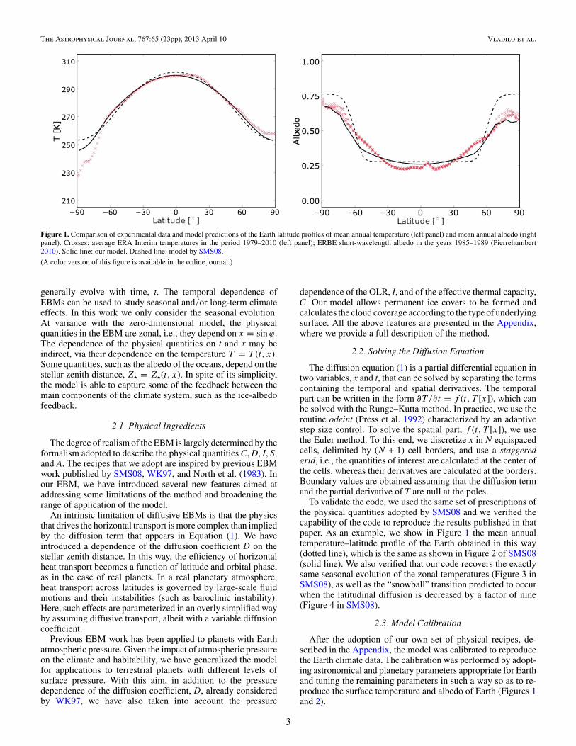
Figure 1. Comparison of experimental data and model predictions of the Earth latitude profiles of mean annual temperature (left panel) and mean annual albedo (rightpanel). Crosses: average ERA Interim temperatures in the period 1979–2010 (left panel); ERBE short-wavelength albedo in the years 1985–1989 (Pierrehumbert2010). Solid line: our model. Dashed line: model by SMS08.
(A color version of this figure is available in the online journal.)
generally evolve with time, t. The temporal dependence ofEBMs can be used to study seasonal and/or long-term climateeffects. In this work we only consider the seasonal evolution.At variance with the zero-dimensional model, the physicalquantities in the EBM are zonal, i.e., they depend on x = sin ϕ.The dependence of the physical quantities on t and x may beindirect, via their dependence on the temperature T = T (t, x).Some quantities, such as the albedo of the oceans, depend on thestellar zenith distance, Z� = Z�(t, x). In spite of its simplicity,the model is able to capture some of the feedback between themain components of the climate system, such as the ice-albedofeedback.
2.1. Physical Ingredients
The degree of realism of the EBM is largely determined by theformalism adopted to describe the physical quantities C, D, I, S,and A. The recipes that we adopt are inspired by previous EBMwork published by SMS08, WK97, and North et al. (1983). Inour EBM, we have introduced several new features aimed ataddressing some limitations of the method and broadening therange of application of the model.
An intrinsic limitation of diffusive EBMs is that the physicsthat drives the horizontal transport is more complex than impliedby the diffusion term that appears in Equation (1). We haveintroduced a dependence of the diffusion coefficient D on thestellar zenith distance. In this way, the efficiency of horizontalheat transport becomes a function of latitude and orbital phase,as in the case of real planets. In a real planetary atmosphere,heat transport across latitudes is governed by large-scale fluidmotions and their instabilities (such as baroclinic instability).Here, such effects are parameterized in an overly simplified wayby assuming diffusive transport, albeit with a variable diffusioncoefficient.
Previous EBM work has been applied to planets with Earthatmospheric pressure. Given the impact of atmospheric pressureon the climate and habitability, we have generalized the modelfor applications to terrestrial planets with different levels ofsurface pressure. With this aim, in addition to the pressuredependence of the diffusion coefficient, D, already consideredby WK97, we have also taken into account the pressure
dependence of the OLR, I, and of the effective thermal capacity,C. Our model allows permanent ice covers to be formed andcalculates the cloud coverage according to the type of underlyingsurface. All the above features are presented in the Appendix,where we provide a full description of the method.
2.2. Solving the Diffusion Equation
The diffusion equation (1) is a partial differential equation intwo variables, x and t, that can be solved by separating the termscontaining the temporal and spatial derivatives. The temporalpart can be written in the form ∂T /∂t = f (t, T [x]), which canbe solved with the Runge–Kutta method. In practice, we use theroutine odeint (Press et al. 1992) characterized by an adaptivestep size control. To solve the spatial part, f (t, T [x]), we usethe Euler method. To this end, we discretize x in N equispacedcells, delimited by (N + 1) cell borders, and use a staggeredgrid, i.e., the quantities of interest are calculated at the center ofthe cells, whereas their derivatives are calculated at the borders.Boundary values are obtained assuming that the diffusion termand the partial derivative of T are null at the poles.
To validate the code, we used the same set of prescriptions ofthe physical quantities adopted by SMS08 and we verified thecapability of the code to reproduce the results published in thatpaper. As an example, we show in Figure 1 the mean annualtemperature–latitude profile of the Earth obtained in this way(dotted line), which is the same as shown in Figure 2 of SMS08(solid line). We also verified that our code recovers the exactlysame seasonal evolution of the zonal temperatures (Figure 3 inSMS08), as well as the “snowball” transition predicted to occurwhen the latitudinal diffusion is decreased by a factor of nine(Figure 4 in SMS08).
2.3. Model Calibration
After the adoption of our own set of physical recipes, de-scribed in the Appendix, the model was calibrated to reproducethe Earth climate data. The calibration was performed by adopt-ing astronomical and planetary parameters appropriate for Earthand tuning the remaining parameters in such a way so as to re-produce the surface temperature and albedo of Earth (Figures 1and 2).
3
The Astrophysical Journal, 767:65 (23pp), 2013 April 10 Vladilo et al.
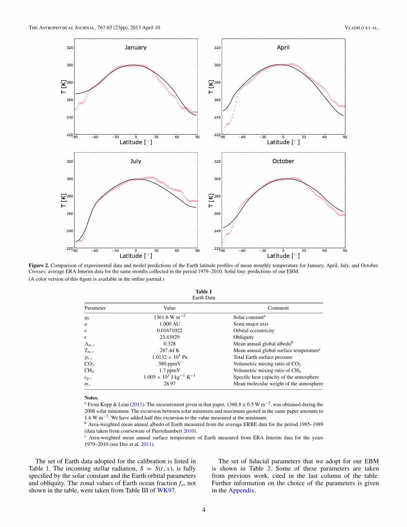
Figure 2. Comparison of experimental data and model predictions of the Earth latitude profiles of mean monthly temperature for January, April, July, and October.Crosses: average ERA Interim data for the same months collected in the period 1979–2010. Solid line: predictions of our EBM.
(A color version of this figure is available in the online journal.)
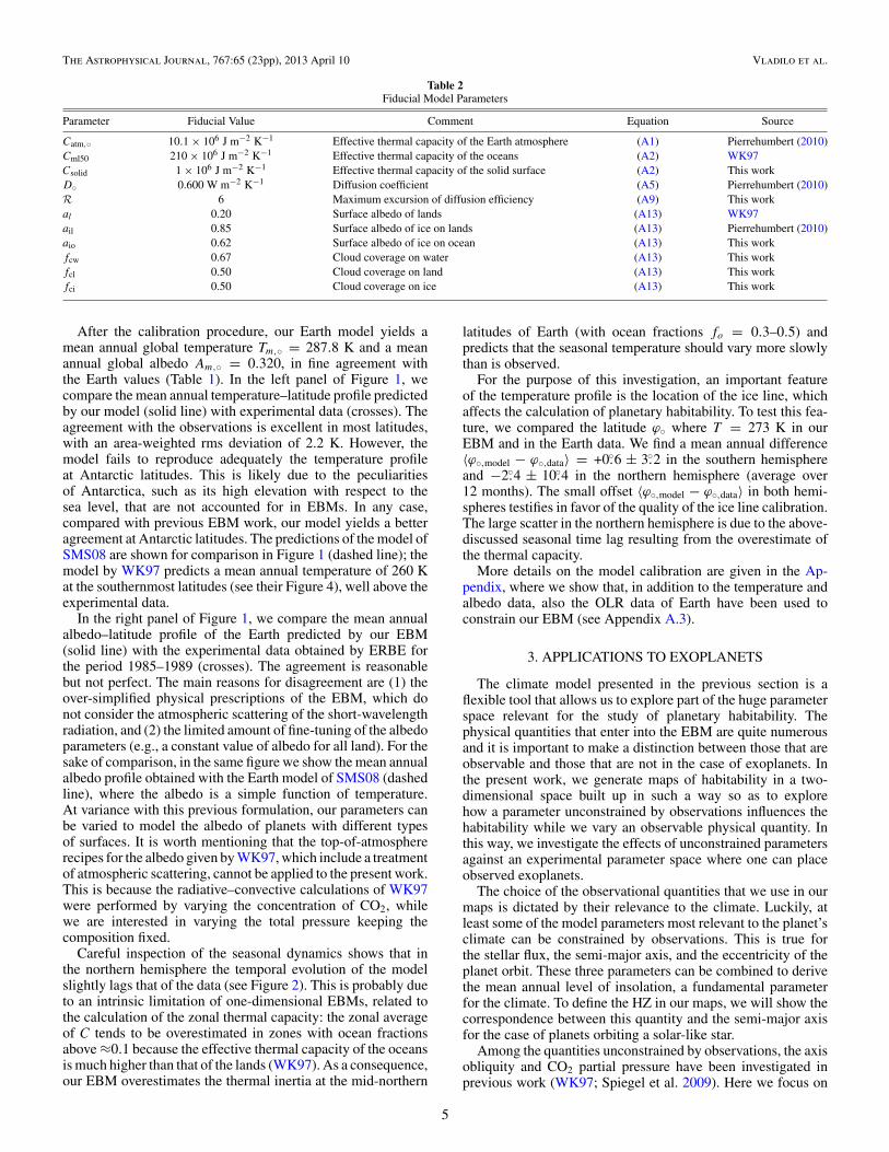
Table 1Earth Data
Parameter Value Comment
q0 1361.6 W m−2 Solar constanta
a 1.000 AU Semi-major axise 0.01671022 Orbital eccentricityε 23.43929 ObliquityAm,◦ 0.328 Mean annual global albedob
Tm,◦ 287.44 K Mean annual global surface temperaturec
pt,◦ 1.0132 × 10⁵ Pa Total Earth surface pressureCO2 380 ppmV Volumetric mixing ratio of CO2
CH4 1.7 ppmV Volumetric mixing ratio of CH4
cp,◦ 1.005 × 10³ J kg−1 K−1 Specific heat capacity of the atmospherem◦ 28.97 Mean molecular weight of the atmosphere
Notes.a From Kopp & Lean (2011). The measurement given in that paper, 1360.8±0.5 W m−2, was obtained during the2008 solar minimum. The excursion between solar minimum and maximum quoted in the same paper amounts to1.6 W m−2. We have added half this excursion to the value measured at the minimum.b Area-weighted mean annual albedo of Earth measured from the average ERBE data for the period 1985–1989(data taken from courseware of Pierrehumbert 2010).c Area-weighted mean annual surface temperature of Earth measured from ERA Interim data for the years1979–2010 (see Dee et al. 2011).
The set of Earth data adopted for the calibration is listed inTable 1. The incoming stellar radiation, S = S(t, x), is fullyspecified by the solar constant and the Earth orbital parametersand obliquity. The zonal values of Earth ocean fraction fo, notshown in the table, were taken from Table III of WK97.
The set of fiducial parameters that we adopt for our EBMis shown in Table 2. Some of these parameters are takenfrom previous work, cited in the last column of the table.Further information on the choice of the parameters is givenin the Appendix.
4
The Astrophysical Journal, 767:65 (23pp), 2013 April 10 Vladilo et al.
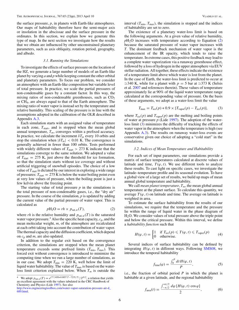
Table 2Fiducial Model Parameters
Parameter Fiducial Value Comment Equation Source
Catm,◦ 10.1 × 10⁶ J m−2 K−1 Effective thermal capacity of the Earth atmosphere (A1) Pierrehumbert (2010)Cml50 210 × 106 J m−2 K−1 Effective thermal capacity of the oceans (A2) WK97Csolid 1 × 10⁶ J m−2 K−1 Effective thermal capacity of the solid surface (A2) This workD◦ 0.600 W m−2 K−1 Diffusion coefficient (A5) Pierrehumbert (2010)R 6 Maximum excursion of diffusion efficiency (A9) This workal 0.20 Surface albedo of lands (A13) WK97ail 0.85 Surface albedo of ice on lands (A13) Pierrehumbert (2010)aio 0.62 Surface albedo of ice on ocean (A13) This workfcw 0.67 Cloud coverage on water (A13) This workfcl 0.50 Cloud coverage on land (A13) This workfci 0.50 Cloud coverage on ice (A13) This work
After the calibration procedure, our Earth model yields amean annual global temperature Tm,◦ = 287.8 K and a meanannual global albedo Am,◦ = 0.320, in fine agreement withthe Earth values (Table 1). In the left panel of Figure 1, wecompare the mean annual temperature–latitude profile predictedby our model (solid line) with experimental data (crosses). Theagreement with the observations is excellent in most latitudes,with an area-weighted rms deviation of 2.2 K. However, themodel fails to reproduce adequately the temperature profileat Antarctic latitudes. This is likely due to the peculiaritiesof Antarctica, such as its high elevation with respect to thesea level, that are not accounted for in EBMs. In any case,compared with previous EBM work, our model yields a betteragreement at Antarctic latitudes. The predictions of the model ofSMS08 are shown for comparison in Figure 1 (dashed line); themodel by WK97 predicts a mean annual temperature of 260 Kat the southernmost latitudes (see their Figure 4), well above theexperimental data.
In the right panel of Figure 1, we compare the mean annualalbedo–latitude profile of the Earth predicted by our EBM(solid line) with the experimental data obtained by ERBE forthe period 1985–1989 (crosses). The agreement is reasonablebut not perfect. The main reasons for disagreement are (1) theover-simplified physical prescriptions of the EBM, which donot consider the atmospheric scattering of the short-wavelengthradiation, and (2) the limited amount of fine-tuning of the albedoparameters (e.g., a constant value of albedo for all land). For thesake of comparison, in the same figure we show the mean annualalbedo profile obtained with the Earth model of SMS08 (dashedline), where the albedo is a simple function of temperature.At variance with this previous formulation, our parameters canbe varied to model the albedo of planets with different typesof surfaces. It is worth mentioning that the top-of-atmosphererecipes for the albedo given by WK97, which include a treatmentof atmospheric scattering, cannot be applied to the present work.This is because the radiative–convective calculations of WK97were performed by varying the concentration of CO2, whilewe are interested in varying the total pressure keeping thecomposition fixed.
Careful inspection of the seasonal dynamics shows that inthe northern hemisphere the temporal evolution of the modelslightly lags that of the data (see Figure 2). This is probably dueto an intrinsic limitation of one-dimensional EBMs, related tothe calculation of the zonal thermal capacity: the zonal averageof C tends to be overestimated in zones with ocean fractionsabove ≈0.1 because the effective thermal capacity of the oceansis much higher than that of the lands (WK97). As a consequence,our EBM overestimates the thermal inertia at the mid-northern
latitudes of Earth (with ocean fractions fo = 0.3–0.5) andpredicts that the seasonal temperature should vary more slowlythan is observed.
For the purpose of this investigation, an important featureof the temperature profile is the location of the ice line, whichaffects the calculation of planetary habitability. To test this fea-ture, we compared the latitude ϕ◦ where T = 273 K in ourEBM and in the Earth data. We find a mean annual difference〈ϕ◦,model − ϕ◦,data〉 = +0.◦6 ± 3.◦2 in the southern hemisphereand −2.◦4 ± 10.◦4 in the northern hemisphere (average over12 months). The small offset 〈ϕ◦,model − ϕ◦,data〉 in both hemi-spheres testifies in favor of the quality of the ice line calibration.The large scatter in the northern hemisphere is due to the above-discussed seasonal time lag resulting from the overestimate ofthe thermal capacity.
More details on the model calibration are given in the Ap-pendix, where we show that, in addition to the temperature andalbedo data, also the OLR data of Earth have been used toconstrain our EBM (see Appendix A.3).
3. APPLICATIONS TO EXOPLANETS
The climate model presented in the previous section is aflexible tool that allows us to explore part of the huge parameterspace relevant for the study of planetary habitability. Thephysical quantities that enter into the EBM are quite numerousand it is important to make a distinction between those that areobservable and those that are not in the case of exoplanets. Inthe present work, we generate maps of habitability in a two-dimensional space built up in such a way so as to explorehow a parameter unconstrained by observations influences thehabitability while we vary an observable physical quantity. Inthis way, we investigate the effects of unconstrained parametersagainst an experimental parameter space where one can placeobserved exoplanets.
The choice of the observational quantities that we use in ourmaps is dictated by their relevance to the climate. Luckily, atleast some of the model parameters most relevant to the planet’sclimate can be constrained by observations. This is true forthe stellar flux, the semi-major axis, and the eccentricity of theplanet orbit. These three parameters can be combined to derivethe mean annual level of insolation, a fundamental parameterfor the climate. To define the HZ in our maps, we will show thecorrespondence between this quantity and the semi-major axisfor the case of planets orbiting a solar-like star.
Among the quantities unconstrained by observations, the axisobliquity and CO2 partial pressure have been investigated inprevious work (WK97; Spiegel et al. 2009). Here we focus on
5
The Astrophysical Journal, 767:65 (23pp), 2013 April 10 Vladilo et al.
the surface pressure, p, in planets with Earth-like atmospheres.Our maps of habitability therefore have the semi-major axisor insolation in the abscissae and the surface pressure in theordinates. In this section, we explain how we generate thistype of map. In the next section we investigate how the resultsthat we obtain are influenced by other unconstrained planetaryparameters, such as axis obliquity, rotation period, geography,and albedo.
3.1. Running the Simulations
To investigate the effects of surface pressure on the location ofthe HZ, we generate a large number of models of an Earth-likeplanet by varying a and p while keeping constant the other orbitaland planetary parameters. To focus our problem, we consideran atmosphere with an Earth-like composition but variable levelof total pressure. In practice, we scale the partial pressures ofnon-condensable gases by a constant factor. In this way, themixing ratios of non-condensable greenhouses, such as CO2or CH4, are always equal to that of the Earth atmosphere. Themixing ratio of water vapor is instead set by the temperature andrelative humidity. This scaling of the pressure is in line with theassumptions adopted in the calibration of the OLR described inAppendix A.3.
Each simulation starts with an assigned value of temperaturein each zone, Tstart, and is stopped when the mean globalannual temperature, Tm, converges within a prefixed accuracy.In practice, we calculate the increment δTm every 10 orbits andstop the simulation when |δTm| < 0.01 K. The convergence isgenerally achieved in fewer than 100 orbits. Tests performedwith widely different values of Tstart > 273 K indicate that thesimulations converge to the same solution. We adopted a valueof Tstart = 275 K, just above the threshold for ice formation,so that the simulation starts without ice coverage and withoutartificial triggering of snowball episodes. The choice of a lowvalue of Tstart is dictated by our interest in exploring a wide rangeof pressures: Tstart = 275 K is below the water boiling point evenat very low values of pressure, when the boiling point is just afew kelvin above the freezing point.
The starting value of total pressure p in the simulations isthe total pressure of non-condensable gases, i.e., the “dry air”pressure. In the course of the simulation, p is updated by addingthe current value of the partial pressure of water vapor. This iscalculated as
pH2O = rh × psat,w(T ), (2)
where rh is the relative humidity and psat,w(T ) is the saturatedwater vapor pressure.4 Also the specific heat capacity, cp, and themean molecular weight, m, of the atmosphere are recalculatedat each orbit taking into account the contribution of water vapor.The thermal capacity and the diffusion coefficient, which dependon cp and m, are also updated.
In addition to the regular exit based on the convergencecriterion, the simulations are stopped when the mean planettemperature exceeds some prefixed limits (Tmin, Tmax). Thisforced exit without convergence is introduced to minimize thecomputing time when we run a large number of simulations, asin our case. We adopt Tmin = 220 K, well below the limit ofliquid water habitability. The value of Tmax is based on the water-loss limit criterion explained below. When Tm is outside the
4 We adopt psat,w(T ) = e(77.3450+0.0057 T −7235/T )/T 8.2, a relation that yieldsan excellent agreement with the values tabulated in the CRC Handbook ofChemistry and Physics (Lide 1997). See alsohttp://www.engineeringtoolbox.com/water-vapor-saturation-pressure-air-d_689.html.
interval (Tmin, Tmax), the simulation is stopped and the indicesof habitability are set to zero.
The existence of a planetary water-loss limit is based onthe following arguments. At a given value of relative humidity,pH2O increases with temperature according to Equation (2)because the saturated pressure of water vapor increases withT. The dominant feedback mechanism of water vapor is theenhancement of the IR opacity, which tends to raise thetemperature. In extreme cases, this positive feedback may lead toa complete water vaporization via a runaway greenhouse effect,followed by a loss of hydrogen in the upper atmosphere via EUVstellar radiation. All together, these effects indicate the existenceof a temperature limit above which water is lost from the planet.In the case of Earth, the water-loss limit is predicted to occur at�340 K, while for a planet with p = 5 bar at �373 K (Selsiset al. 2007 and references therein). These values of temperatureapproximately lie at 90% of the liquid water temperature rangecalculated at the corresponding value of pressure. On the basisof these arguments, we adopt as a water-loss limit the value
Tmax = Tice(p) + 0.9 × [Tvapor(p) − Tice(p)], (3)
where Tice(p) and Tvapor(p) are the melting and boiling pointsof water at pressure p (Lide 1997). The adoption of the water-loss limit (3) minimizes the difficulty of tracking the effects ofwater vapor in the atmosphere when the temperature is high (seeAppendix A.3). The results on runaway water-loss events areconservative given our choice of adopting a “cold start” in thesimulations.
3.2. Indices of Mean Temperature and Habitability
For each set of input parameters, our simulations provide amatrix of surface temperatures calculated at discrete values oflatitude and time, T (ϕ, t). We use different tools to analyzethese results. To cast light on specific cases, we investigate thelatitude–temperature profile and its seasonal evolution. To havea global view of a large set of results, we build up maps of meanannual global temperature and habitability.
We call mean planet temperature, Tm, the mean global annualtemperature at the planet surface. To calculate this quantity, weaverage T (ϕ, t) on latitude and time. The average on latitude isweighted in area.
To estimate the surface habitability from the results of oursimulations, we require that the temperature and the pressurelie within the range of liquid water in the phase diagram ofH2O. We consider values of total pressure above the triple pointand below the critical pressure. Within this interval, we definea habitability function such that
H (ϕ, t) ={
1 if Tice(p) � T (ϕ, t) � Tvapor(p)0 otherwise. (4)
Several indices of surface habitability can be defined byintegrating H (ϕ, t) in different ways. Following SMS08, weintroduce the temporal habitability
ftime(ϕ) =∫ P
0 dtH (ϕ, t)
P, (5)
i.e., the fraction of orbital period P in which the planet ishabitable at a given latitude, and the regional habitability
farea(t) =∫ +π/2−π/2 dϕ [H (ϕ, t) cos ϕ]
2, (6)
6
The Astrophysical Journal, 767:65 (23pp), 2013 April 10 Vladilo et al.
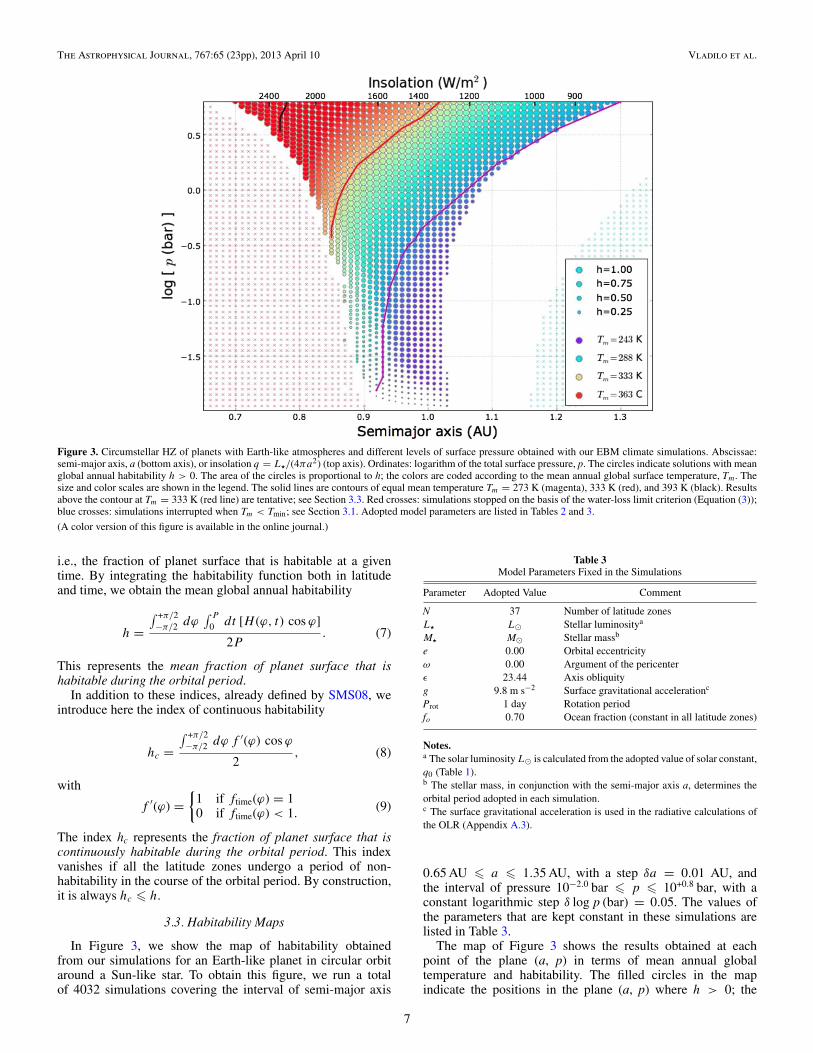
Figure 3. Circumstellar HZ of planets with Earth-like atmospheres and different levels of surface pressure obtained with our EBM climate simulations. Abscissae:semi-major axis, a (bottom axis), or insolation q = L�/(4πa2) (top axis). Ordinates: logarithm of the total surface pressure, p. The circles indicate solutions with meanglobal annual habitability h > 0. The area of the circles is proportional to h; the colors are coded according to the mean annual global surface temperature, Tm. Thesize and color scales are shown in the legend. The solid lines are contours of equal mean temperature Tm = 273 K (magenta), 333 K (red), and 393 K (black). Resultsabove the contour at Tm = 333 K (red line) are tentative; see Section 3.3. Red crosses: simulations stopped on the basis of the water-loss limit criterion (Equation (3));blue crosses: simulations interrupted when Tm < Tmin; see Section 3.1. Adopted model parameters are listed in Tables 2 and 3.
(A color version of this figure is available in the online journal.)
i.e., the fraction of planet surface that is habitable at a giventime. By integrating the habitability function both in latitudeand time, we obtain the mean global annual habitability
h =∫ +π/2−π/2 dϕ
∫ P
0 dt [H (ϕ, t) cos ϕ]
2P. (7)
This represents the mean fraction of planet surface that ishabitable during the orbital period.
In addition to these indices, already defined by SMS08, weintroduce here the index of continuous habitability
hc =∫ +π/2−π/2 dϕ f ′(ϕ) cos ϕ
2, (8)
with
f ′(ϕ) ={
1 if ftime(ϕ) = 10 if ftime(ϕ) < 1.
(9)
The index hc represents the fraction of planet surface that iscontinuously habitable during the orbital period. This indexvanishes if all the latitude zones undergo a period of non-habitability in the course of the orbital period. By construction,it is always hc � h.
3.3. Habitability Maps
In Figure 3, we show the map of habitability obtainedfrom our simulations for an Earth-like planet in circular orbitaround a Sun-like star. To obtain this figure, we run a totalof 4032 simulations covering the interval of semi-major axis
Table 3Model Parameters Fixed in the Simulations
Parameter Adopted Value Comment
N 37 Number of latitude zonesL� L Stellar luminositya
M� M Stellar massb
e 0.00 Orbital eccentricityω 0.00 Argument of the pericenterε 23.44 Axis obliquityg 9.8 m s−2 Surface gravitational accelerationc
Prot 1 day Rotation periodfo 0.70 Ocean fraction (constant in all latitude zones)
Notes.a The solar luminosity L is calculated from the adopted value of solar constant,q0 (Table 1).b The stellar mass, in conjunction with the semi-major axis a, determines theorbital period adopted in each simulation.c The surface gravitational acceleration is used in the radiative calculations ofthe OLR (Appendix A.3).
0.65 AU � a � 1.35 AU, with a step δa = 0.01 AU, andthe interval of pressure 10−2.0 bar � p � 10+0.8 bar, with aconstant logarithmic step δ log p (bar) = 0.05. The values ofthe parameters that are kept constant in these simulations arelisted in Table 3.
The map of Figure 3 shows the results obtained at eachpoint of the plane (a, p) in terms of mean annual globaltemperature and habitability. The filled circles in the mapindicate the positions in the plane (a, p) where h > 0; the
7
The Astrophysical Journal, 767:65 (23pp), 2013 April 10 Vladilo et al.
value of total pressure associated to these symbols includesthe partial pressure of water vapor updated in the courseof the simulation. Crosses indicate positions on the plane wherethe simulations were forced to exit; the total pressure for thesecases is the starting value of dry air pressure (see Section 3.1).Empty areas of the map, as well as crosses, indicate a locationof non-habitability.
The simulations yield information not only on the degree ofhabitability, through the index h, but also on the “quality” ofthe habitability, through a detailed analysis of the seasonal andlatitudinal variations of the temperature, as we shall see in thenext section. However, some cautionary remarks must be madebefore interpreting these data.
The model has been calibrated using Earth climatologicaldata. These data span a range of temperatures, roughly 220 K� T � 310 K, not sufficient to cover the broad diversityexpected for exoplanets, even if we just consider those ofterrestrial type. Given the fundamental role of temperaturein the diffusion equation, one should be careful in using thephysical quantities outside this range, where direct calibrationis not possible. In this respect, the major reason of concernis the estimate of the OLR that has been done with radiativecalculations (see Appendix A.3). The difficulty of calibratingthe OLR outside the range of terrestrial temperatures makesuncertain the exact localization of the inner and outer edges ofthe HZ. In particular, the results with Tm � 330 K should betreated with caution, given the strong effects of water vaporpredicted to occur in this temperature range, which are notdirectly testable. These cases lie in the region of high pressurein Figure 3 (symbols color-coded in orange and red). The factthat in these cases also the pressure is quite different from theEarth value makes these results particularly uncertain. In thefollowing discussion, we will consider these particular resultsto be purely tentative. We note that the difficulty of makingclimate predictions outside the parameter space sampled by theEarth is a common problem of any type of climate model, nomatter how sophisticated. In this respect, simple models, likeour EBM, help to obtain preliminary predictions to be tested bysubsequent investigations.
4. DISCUSSION
In this section, we describe and interpret the complex patternsthat we find in the pressure-dependent map of planet temperatureand habitability of Figure 3. We then discuss how the results canbe extended to more general situations other than circular orbitsof planets orbiting a Sun-like star. We conclude this sectionsetting our results in the context of previous studies.
4.1. The Pressure-dependent Habitable Zone
The circumstellar HZ shown in Figure 3 shows several char-acteristics, in terms of mean planet temperature and habitability,that can be summarized as follows.
The radial extent of the HZ increases with p. The outer edgeextends from 1.02 to 1.18 AU when the pressure rises from 0.1to 3 bar. The inner edge approaches the star from 0.87 to 0.77AU in the same pressure interval. No habitability is found belowp � 15 mbar.
The broadening of the HZ with increasing pressure is accom-panied by an increase of the interval of mean planet temperaturesspanned at constant p. At high pressures, most of the broadeningof the HZ is contributed by the area of the plane where the so-lutions have mean temperatures Tm � 60◦C (i.e., Tm � 333 K;
orange and red symbols above the red line in the figure). If wefocus on the interval of mean temperatures 0◦C � Tm � 60◦C(region with 273 K � Tm � 333 K between the magenta andred line), the broadening of the HZ is quite modest.
Remarkable differences exist between the low- and high-pressure regimes. At low pressures (p � 0.3 bar) the habitabilityundergoes intense variations in the plane (a, p), with a generaltrend of increasing h with increasing p. At high pressure (p �1 bar) the habitability is approximately constant and high, withsudden transitions from h � 1 inside the HZ, to h � 0. The meanplanet temperature also shows different characteristics betweenthe low- and high-pressure regimes. Starting from pressurep � 0.3 bar, the curves of equal temperature tend to moveaway from the star as the pressure increases. This behavior isnot seen at lower pressures, where the HZ at a given temperaturedoes not significantly change its distance from the star.
Another interesting feature of Figure 3 is the location of theline of constant mean planet temperature Tm = 273 K, indicatedas a magenta solid line superimposed on the symbols of hab-itability. On the basis of the liquid water habitability criterion,one would expect a coincidence of this line with the outer edgeof the HZ. This is true at p � 2 bar, but not at lower values ofpressure, the mismatch being quite large at the lowest valuesof pressure considered. The reason is that, using an EBM, wecan determine whether some latitudinal zones have tempera-tures larger than zero, even when the mean planet temperatureis lower. When this is the case, the planet is partly habitable.
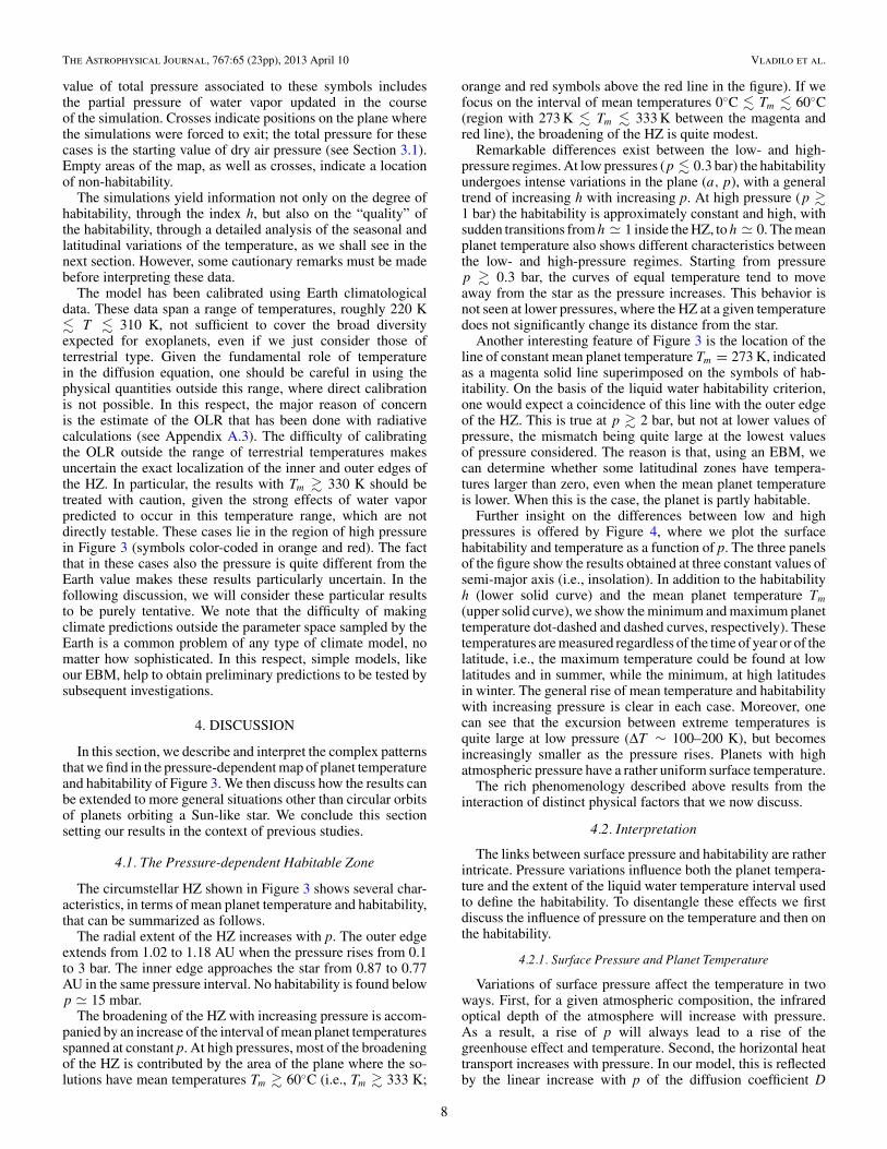
Further insight on the differences between low and highpressures is offered by Figure 4, where we plot the surfacehabitability and temperature as a function of p. The three panelsof the figure show the results obtained at three constant values ofsemi-major axis (i.e., insolation). In addition to the habitabilityh (lower solid curve) and the mean planet temperature Tm(upper solid curve), we show the minimum and maximum planettemperature dot-dashed and dashed curves, respectively). Thesetemperatures are measured regardless of the time of year or of thelatitude, i.e., the maximum temperature could be found at lowlatitudes and in summer, while the minimum, at high latitudesin winter. The general rise of mean temperature and habitabilitywith increasing pressure is clear in each case. Moreover, onecan see that the excursion between extreme temperatures isquite large at low pressure (ΔT ∼ 100–200 K), but becomesincreasingly smaller as the pressure rises. Planets with highatmospheric pressure have a rather uniform surface temperature.
The rich phenomenology described above results from theinteraction of distinct physical factors that we now discuss.
4.2. Interpretation
The links between surface pressure and habitability are ratherintricate. Pressure variations influence both the planet tempera-ture and the extent of the liquid water temperature interval usedto define the habitability. To disentangle these effects we firstdiscuss the influence of pressure on the temperature and then onthe habitability.
4.2.1. Surface Pressure and Planet Temperature
Variations of surface pressure affect the temperature in twoways. First, for a given atmospheric composition, the infraredoptical depth of the atmosphere will increase with pressure.As a result, a rise of p will always lead to a rise of thegreenhouse effect and temperature. Second, the horizontal heattransport increases with pressure. In our model, this is reflectedby the linear increase with p of the diffusion coefficient D
8
The Astrophysical Journal, 767:65 (23pp), 2013 April 10 Vladilo et al.
Figure 4. Planet surface temperature, T, and habitability, h, as a function ofsurface pressure, p. Each panel shows the results obtained at constant semi-major axis, a, and constant insolation, q, indicated in the legend. The solidcurve at the bottom of each panel is the habitability expressed in percent units.The three curves at the top of each panel are temperature curves in kelvin units(solid line: mean planet temperature; dot-dashed and dashed lines: minimumand maximum planet temperatures at any latitude and season). Adopted modelparameters are listed in Tables 2 and 3.
(A color version of this figure is available in the online journal.)
(Equation (A5), Appendix A.2). At variance with the first effect,it is not straightforward to predict how the temperature will reactto a variation of the horizontal transport.
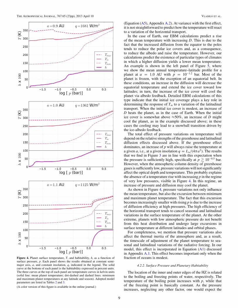
In the case of Earth, our EBM calculations predict a riseof the mean temperature with increasing D. This is due to thefact that the increased diffusion from the equator to the polestends to reduce the polar ice covers and, as a consequence,to reduce the albedo and raise the temperature. However, ourcalculations predict the existence of particular types of climatesin which a higher diffusion yields a lower mean temperature.An example is shown in the left panel of Figure 5, wherewe show the mean annual temperature–latitude profile for aplanet at a = 1.0 AU with p = 10−1.2 bar. Most of theplanet is frozen, with the exception of an equatorial belt. Inthese conditions, an increase in the diffusion will decrease theequatorial temperature and extend the ice cover toward lowlatitudes; in turn, the increase of the ice cover will cool theplanet via albedo feedback. Detailed EBM calculations of thistype indicate that the initial ice coverage plays a key role indetermining the response of Tm to a variation of the latitudinaltransport. When the initial ice cover is modest, an increase ofD heats the planet, as in the case of Earth. When the initialice cover is somewhat above ≈50%, an increase of D mightcool the planet, as in the example discussed above; in thesecases the cooling may lead to a snowball transition driven bythe ice-albedo feedback.
The total effect of pressure variations on temperature willdepend on the relative strengths of the greenhouse and latitudinaldiffusion effects discussed above. If the greenhouse effectdominates, an increase of p will always raise the temperature ata given a, i.e., at a given insolation q = L�/(4πa2). The resultsthat we find in Figure 3 are in line with this expectation whenthe pressure is sufficiently high, specifically at p � 10−0.5 bar.However, when the atmospheric column density of greenhousegases is sufficiently low, pressure variations will not significantlyaffect the optical depth and temperature. This probably explainsthe absence of a temperature rise with increasing p in the regimeof very low pressures, visible in Figure 4. In this regime, anincrease of pressure and diffusion may cool the planet.
As shown in Figure 4, pressure variations not only influencethe mean temperature, but also the excursion between minimumand maximum planet temperature. The fact that this excursionbecomes increasingly smaller with rising p is due to the increaseof diffusion efficiency at high pressures. The high efficiency ofthe horizontal transport tends to cancel seasonal and latitudinalvariations in the surface temperature of the planet. At the otherextreme, planets with low atmospheric pressure do not benefitfrom this heat distribution and undergo large excursions insurface temperature at different latitudes and orbital phases.
For completeness, we mention that pressure variations alsoaffect the thermal inertia of the atmosphere and, as a result,the timescale of adjustment of the planet temperature to sea-sonal and latitudinal variations of the radiative forcing. In ourmodel, this effect is incorporated in Equation (A1) discussedin Appendix A.1. This effect becomes important only when thefraction of oceans is modest.
4.2.2. Surface Pressure and Planetary Habitability
The location of the inner and outer edges of the HZ is relatedto the boiling and freezing points of water, respectively. Thetemperature of the boiling point increases with p, while thatof the freezing point is basically constant. As the pressureincreases, neglecting any other factor, one would expect the
9
The Astrophysical Journal, 767:65 (23pp), 2013 April 10 Vladilo et al.
Figure 5. Solid curve: mean annual temperature–latitude profile of an Earth-like planet with semi-major axis, a, surface pressure, p, and habitability, h, specified inthe legend of each panel. Solid horizontal line: mean annual global temperature, Tm. Dashed horizontal lines: liquid water temperature interval at pressure p. Adoptedmodel parameters are listed in Tables 2 and 3. Temperature–latitude profiles are symmetric as a result of the idealized geography used in the simulation (constantfraction of oceans in all latitude zones). Crosses: Earth data as in Figure 1.
(A color version of this figure is available in the online journal.)
inner edge of the HZ to approach the star and the outer edgeto stay at a ≈ constant. The inner edge of the HZ in Figure 3confirms this expectation. The outer edge, instead, moves awayfrom the star as the pressure increases. This is due to thepressure–temperature effects described above: at high pressurethe greenhouse effect becomes more important with increasing pand the planet can remain above the freezing point at increasinga. At the inner edge, the rise of the boiling point dominates overthe pressure–temperature effects. For considerations about thekind of life that can be expected at these high temperatures, seeSection 4.5.2.
At low pressures the situation is quite complicated. Whenp � 2 bar, the contour with Tm = 273 K (magenta line in thefigure) does not overlap with the outer edge of the HZ. In fact,there is an area of the plane (a, p) where planets are habitableeven if Tm is below freezing point. This can be understood fromthe analysis of the latitude–temperature profiles of planets lyingin this area of the map. The example at a = 1.0 AU withp = 10−1.2 bar (left panel of Figure 5) explains this apparentdiscrepancy. As one can see, even if the mean temperature Tm(solid horizontal line) is below freezing point (lower horizontaldashed line) the existence of a tropical zone of the planetwith temperatures above freezing point yields a habitabilityh = 0.33.
Another peculiar feature of Figure 3 is the existence ofplanets with Tm well inside the liquid water range but withlow levels of habitability. An example of this type is shown inthe right panel of Figure 5. The mean temperature Tm (solidhorizontal line) lies between the freezing and boiling points(horizontal dashed lines), but the habitability is only h = 0.24.The temperature–latitude profile explains the reason for this lowhabitability: most of the planet surface lies outside the liquid-water range because the equatorial belt is above the boiling pointand the high latitude zones below the freezing point.
These examples clearly indicate that the mean planet tem-perature is not a good indicator of habitability when the planetpressure is low.
The pressure dependence of the horizontal heat transport alsoplays an important role in determining the characteristics ofhabitability. As discussed above, planets with high pressure have
a uniform surface temperature as a result of the high diffusion.The consequence in terms of habitability is that all the planetsurface is either within or outside the liquid water temperaturerange. If a planet with high pressure lies inside the HZ, itshabitability will be h � 1. If the temperature goes outsidethe liquid water range, all the planet surface will become un-habitable. This explains the sudden transitions from h � 1 toh � 0 that we see in the upper part of Figure 3 when we go outof the HZ.
4.3. Effects of Physical Quantities Constrainedby Observations
In addition to the semi-major axis, the orbital eccentricityand the stellar properties can be measured in the frameworkof observational studies and are relevant for the climate andhabitability of exoplanets. The results shown in Figure 3 havebeen derived for circular orbits and solar-type stars. Here wediscuss the extent to which we can generalize these results foreccentric orbits and non-solar-type stars.
4.3.1. Eccentric Orbits
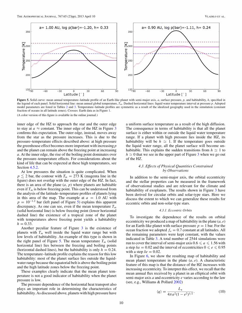
To investigate the dependence of the results on orbitaleccentricity we produced a map of habitability in the plane (a, e)for an Earth-like planet with surface pressure p = 1 bar. For theocean fraction we adopted fo = 0.7 constant at all latitudes. Allthe remaining parameters were kept constant, with the valuesindicated in Table 3. A total number of 2544 simulations wererun to cover the interval of semi-major axis 0.6 � a � 1.56 witha step δa = 0.02 and the interval of eccentricities 0 � e � 0.95with a step δe = 0.02.
In Figure 6, we show the resulting map of habitability andmean planet temperature in the plane (a, e). A characteristicfeature of this map is that the distance of the HZ increases withincreasing eccentricity. To interpret this effect, we recall that themean annual flux received by a planet in an elliptical orbit withsemi-major axis a and eccentricity e varies according to the law(see, e.g., Williams & Pollard 2002)
〈q〉 = L�
4πa2(1 − e2)1/2. (10)
10
The Astrophysical Journal, 767:65 (23pp), 2013 April 10 Vladilo et al.
Figure 6. Maps of mean temperature and habitability of an Earth-like planet in the plane of the semi-major axis and eccentricity. Left panel: habitability h; right panel:continuous habitability hc (see Section 3.2). The area of the circles is proportional to the mean fractional habitability; the color varies according to the mean annualglobal surface temperature, Tm. The size and color scales are shown in the legend. Adopted model parameters are listed in Tables 2 and 3, with the exception of theeccentricity that has been varied as shown in the figure. Solid curve: line of equal mean annual flux 〈q〉 = q0 estimated from Equation (10).
(A color version of this figure is available in the online journal.)
Therefore, compared to a circular orbit of radius a and constantinsolation q0 = L�/4πa2, the mean annual flux in an eccentricorbit increases with e according to the relation 〈q〉 = q0(1 −e2)−1/2. In turn, this increase of mean flux is expected to raise themean temperature Tm. This is indeed what we find in the resultsof the simulations. The rise of Tm at constant a can be appreciatedin the figure, where the symbols are color-coded according to Tm.To test this effect in a quantitative way, we superimpose on thefigure the curve of constant mean flux 〈q〉 = q0, calculated fromEquation (10) for L� = L. One can see that the HZ followsthe same type of functional dependence, e ∝ (1 − a−4)1/2, ofthe curve calculated at constant flux. This result confirms that theincrease of mean annual flux is the main effect that governs theshift of the HZ to larger distances from the star as the eccentricityincreases.
A second characteristic feature of Figure 6 is that thehabitability tends to decrease with increasing eccentricity. Thiseffect is more evident when we consider the map of continuoushabitability, hc, in the right panel of the figure. The effect isrelated to the large excursion of the instantaneous stellar fluxalong orbits that are very elongated. The maximum excursionof the flux grows as [(1 + e)/(1 − e)]2, and therefore exceedsone order of magnitude when e > 0.5. As a consequenceof this strong flux variation, the fraction of orbital period inwhich the planet is habitable at a given latitude must becomeincreasingly smaller as the orbit becomes more elongated. Thisis equivalent to saying that ftime(ϕ) decreases and therefore alsoh and hc decrease (Section 3.2) with increasing e. The effect onhc must be stronger because this quantity depends on ftime(ϕ)via Equation (9). The comparison between the left and rightpanels of Figure 6 indicates the existence of an area of the plane(a, e), at high values of a and e, populated by planets that arehabitable in small fractions of their orbit. This is demonstratedby the fact that such a population disappears when we consider
the continuous habitability hc. Apart from the existence of thisarea, it is clear from these figures that the radial extent of theHZ tends to decrease with increasing eccentricity.
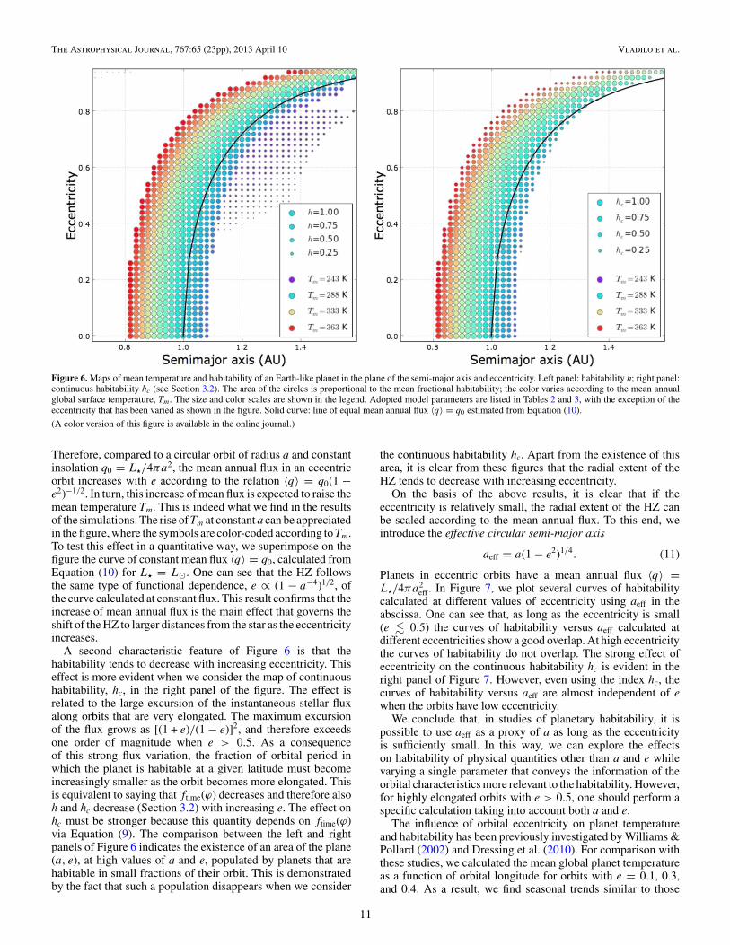
On the basis of the above results, it is clear that if theeccentricity is relatively small, the radial extent of the HZ canbe scaled according to the mean annual flux. To this end, weintroduce the effective circular semi-major axis
aeff = a(1 − e2)1/4. (11)
Planets in eccentric orbits have a mean annual flux 〈q〉 =L�/4πa2
eff . In Figure 7, we plot several curves of habitabilitycalculated at different values of eccentricity using aeff in theabscissa. One can see that, as long as the eccentricity is small(e � 0.5) the curves of habitability versus aeff calculated atdifferent eccentricities show a good overlap. At high eccentricitythe curves of habitability do not overlap. The strong effect ofeccentricity on the continuous habitability hc is evident in theright panel of Figure 7. However, even using the index hc, thecurves of habitability versus aeff are almost independent of ewhen the orbits have low eccentricity.
We conclude that, in studies of planetary habitability, it ispossible to use aeff as a proxy of a as long as the eccentricityis sufficiently small. In this way, we can explore the effectson habitability of physical quantities other than a and e whilevarying a single parameter that conveys the information of theorbital characteristics more relevant to the habitability. However,for highly elongated orbits with e > 0.5, one should perform aspecific calculation taking into account both a and e.
The influence of orbital eccentricity on planet temperatureand habitability has been previously investigated by Williams &Pollard (2002) and Dressing et al. (2010). For comparison withthese studies, we calculated the mean global planet temperatureas a function of orbital longitude for orbits with e = 0.1, 0.3,and 0.4. As a result, we find seasonal trends similar to those
11
The Astrophysical Journal, 767:65 (23pp), 2013 April 10 Vladilo et al.
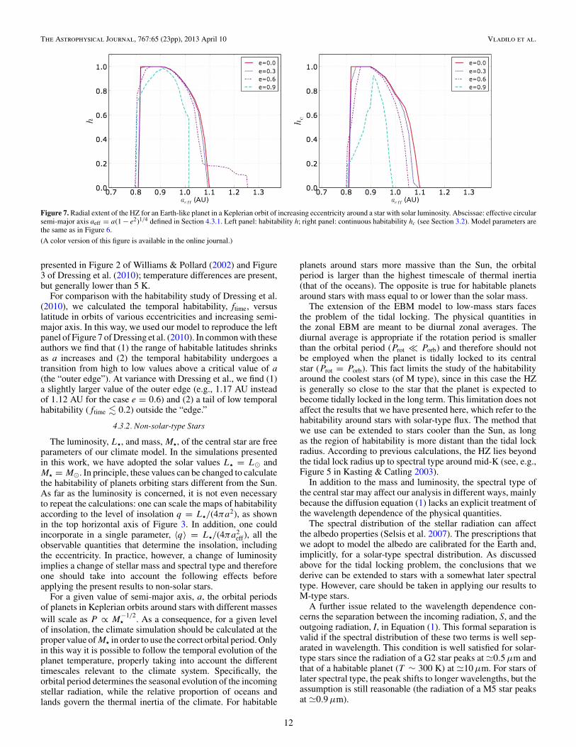
Figure 7. Radial extent of the HZ for an Earth-like planet in a Keplerian orbit of increasing eccentricity around a star with solar luminosity. Abscissae: effective circularsemi-major axis aeff = a(1 − e2)1/4 defined in Section 4.3.1. Left panel: habitability h; right panel: continuous habitability hc (see Section 3.2). Model parameters arethe same as in Figure 6.
(A color version of this figure is available in the online journal.)
presented in Figure 2 of Williams & Pollard (2002) and Figure3 of Dressing et al. (2010); temperature differences are present,but generally lower than 5 K.
For comparison with the habitability study of Dressing et al.(2010), we calculated the temporal habitability, ftime, versuslatitude in orbits of various eccentricities and increasing semi-major axis. In this way, we used our model to reproduce the leftpanel of Figure 7 of Dressing et al. (2010). In common with theseauthors we find that (1) the range of habitable latitudes shrinksas a increases and (2) the temporal habitability undergoes atransition from high to low values above a critical value of a(the “outer edge”). At variance with Dressing et al., we find (1)a slightly larger value of the outer edge (e.g., 1.17 AU insteadof 1.12 AU for the case e = 0.6) and (2) a tail of low temporalhabitability (ftime � 0.2) outside the “edge.”
4.3.2. Non-solar-type Stars
The luminosity, L�, and mass, M�, of the central star are freeparameters of our climate model. In the simulations presentedin this work, we have adopted the solar values L� = L andM� = M. In principle, these values can be changed to calculatethe habitability of planets orbiting stars different from the Sun.As far as the luminosity is concerned, it is not even necessaryto repeat the calculations: one can scale the maps of habitabilityaccording to the level of insolation q = L�/(4πa2), as shownin the top horizontal axis of Figure 3. In addition, one couldincorporate in a single parameter, 〈q〉 = L�/(4πa2
eff), all theobservable quantities that determine the insolation, includingthe eccentricity. In practice, however, a change of luminosityimplies a change of stellar mass and spectral type and thereforeone should take into account the following effects beforeapplying the present results to non-solar stars.
For a given value of semi-major axis, a, the orbital periodsof planets in Keplerian orbits around stars with different masseswill scale as P ∝ M
−1/2� . As a consequence, for a given level
of insolation, the climate simulation should be calculated at theproper value of M� in order to use the correct orbital period. Onlyin this way it is possible to follow the temporal evolution of theplanet temperature, properly taking into account the differenttimescales relevant to the climate system. Specifically, theorbital period determines the seasonal evolution of the incomingstellar radiation, while the relative proportion of oceans andlands govern the thermal inertia of the climate. For habitable
planets around stars more massive than the Sun, the orbitalperiod is larger than the highest timescale of thermal inertia(that of the oceans). The opposite is true for habitable planetsaround stars with mass equal to or lower than the solar mass.
The extension of the EBM model to low-mass stars facesthe problem of the tidal locking. The physical quantities inthe zonal EBM are meant to be diurnal zonal averages. Thediurnal average is appropriate if the rotation period is smallerthan the orbital period (Prot � Porb) and therefore should notbe employed when the planet is tidally locked to its centralstar (Prot = Porb). This fact limits the study of the habitabilityaround the coolest stars (of M type), since in this case the HZis generally so close to the star that the planet is expected tobecome tidally locked in the long term. This limitation does notaffect the results that we have presented here, which refer to thehabitability around stars with solar-type flux. The method thatwe use can be extended to stars cooler than the Sun, as longas the region of habitability is more distant than the tidal lockradius. According to previous calculations, the HZ lies beyondthe tidal lock radius up to spectral type around mid-K (see, e.g.,Figure 5 in Kasting & Catling 2003).
In addition to the mass and luminosity, the spectral type ofthe central star may affect our analysis in different ways, mainlybecause the diffusion equation (1) lacks an explicit treatment ofthe wavelength dependence of the physical quantities.
The spectral distribution of the stellar radiation can affectthe albedo properties (Selsis et al. 2007). The prescriptions thatwe adopt to model the albedo are calibrated for the Earth and,implicitly, for a solar-type spectral distribution. As discussedabove for the tidal locking problem, the conclusions that wederive can be extended to stars with a somewhat later spectraltype. However, care should be taken in applying our results toM-type stars.
A further issue related to the wavelength dependence con-cerns the separation between the incoming radiation, S, and theoutgoing radiation, I, in Equation (1). This formal separation isvalid if the spectral distribution of these two terms is well sep-arated in wavelength. This condition is well satisfied for solar-type stars since the radiation of a G2 star peaks at �0.5 μm andthat of a habitable planet (T ∼ 300 K) at �10 μm. For stars oflater spectral type, the peak shifts to longer wavelengths, but theassumption is still reasonable (the radiation of a M5 star peaksat �0.9 μm).
12
The Astrophysical Journal, 767:65 (23pp), 2013 April 10 Vladilo et al.
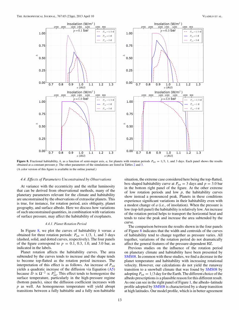
Figure 8. Fractional habitability, h, as a function of semi-major axis, a, for planets with rotation periods Prot = 1/3, 1, and 3 days. Each panel shows the resultsobtained at a constant pressure p. The other parameters of the simulations are listed in Tables 2 and 3.
(A color version of this figure is available in the online journal.)
4.4. Effects of Parameters Unconstrained by Observations
At variance with the eccentricity and the stellar luminositythat can be derived from observational methods, many of theplanetary parameters relevant for the climate and habitabilityare unconstrained by the observations of extrasolar planets. Thisis true, for instance, for rotation period, axis obliquity, planetgeography, and surface albedo. Here we discuss how variationsof such unconstrained quantities, in combination with variationsof surface pressure, may affect the habitability of exoplanets.
4.4.1. Planet Rotation Period
In Figure 8, we plot the curves of habitability h versus aobtained for three rotation periods: Prot = 1/3, 1, and 3 days(dashed, solid, and dotted curves, respectively). The four panelsof the figure correspond to p = 0.1, 0.3, 1.0, and 3.0 bar, asindicated in the labels.
Planet rotation affects the habitability curves. The areasubtended by the curves tends to increase and the shape tendsto become top-flatted as the rotation period increases. Theinterpretation of this effect is as follows. An increase of Protyields a quadratic increase of the diffusion via Equation (A5)because D ∝ Ω−2 ∝ P 2
rot. This effect tends to homogenize thesurface temperature, particularly in the high-pressure regime(bottom panels), since the diffusion coefficient increases withp as well. An homogeneous temperature will yield abrupttransitions between a fully habitable and a fully non-habitable
situation, the extreme case considered here being the top-flatted,box-shaped habitability curve at Prot = 3 days and p = 3.0 barin the bottom right panel of the figure. At the other extremeof low rotation periods and low p, the habitability curvesshow instead a pronounced peak. Planets in these conditionsexperience significant variations in their habitability even witha modest change of a (i.e., of insolation). When the pressure islow (top-left panel) the habitability is relatively low. An increaseof the rotation period helps to transport the horizontal heat andtends to raise the peak and increase the area subtended by thecurve.
The comparison between the results shown in the four panelsof Figure 8 indicates that the width and centroids of the curvesof habitability tend to change together as pressure varies. Alltogether, variations of the rotation period do not dramaticallyaffect the general features of the pressure-dependent HZ.
Previous studies on the influence of the rotation periodon planetary climate and habitability have been presented bySMS08. In common with these studies, we find a decrease in theplanet temperature and habitability with increasing rotationalvelocity. However, our calculations do not yield the runawaytransition to a snowball climate that was found by SMS08 byadopting Prot = 1/3 day for the Earth. The different choice of thealbedo prescriptions is a plausible reason for this different result.As one can see in the right panel of Figure 1, the albedo–latitudeprofile adopted by SMS08 is characterized by a sharp transitionat high latitudes. Our model profile, which is in better agreement
13
The Astrophysical Journal, 767:65 (23pp), 2013 April 10 Vladilo et al.
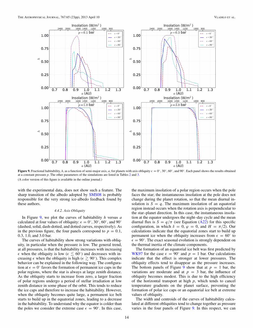
Figure 9. Fractional habitability, h, as a function of semi-major axis, a, for planets with axis obliquity ε = 0◦, 30◦, 60◦, and 90◦. Each panel shows the results obtainedat a constant pressure p. The other parameters of the simulations are listed in Tables 2 and 3.
(A color version of this figure is available in the online journal.)
with the experimental data, does not show such a feature. Thesharp transition of the albedo adopted by SMS08 is probablyresponsible for the very strong ice-albedo feedback found bythese authors.
4.4.2. Axis Obliquity
In Figure 9, we plot the curves of habitability h versus acalculated at four values of obliquity: ε = 0◦, 30◦, 60◦, and 90◦(dashed, solid, dash-dotted, and dotted curves, respectively). Asin the previous figure, the four panels correspond to p = 0.1,0.3, 1.0, and 3.0 bar.
The curves of habitability show strong variations with obliq-uity, in particular when the pressure is low. The general trend,at all pressures, is that the habitability increases with increasingε when the obliquity is low (ε � 60◦) and decreases with in-creasing ε when the obliquity is high (ε � 90◦). This complexbehavior can be explained in the following way. The configura-tion at ε = 0◦ favors the formation of permanent ice caps in thepolar regions, where the star is always at large zenith distance.As the obliquity starts to increase from zero, a larger fractionof polar regions undergo a period of stellar irradiation at lowzenith distance in some phase of the orbit. This tends to reducethe ice caps and therefore to increase the habitability. However,when the obliquity becomes quite large, a permanent ice beltstarts to build up in the equatorial zones, leading to a decreasein the habitability. To understand why the equator is colder thanthe poles we consider the extreme case ε = 90◦. In this case,
the maximum insolation of a polar region occurs when the polefaces the star; the instantaneous insolation at the pole does notchange during the planet rotation, so that the mean diurnal in-solation is S = q. The maximum insolation of an equatorialregion instead occurs when the rotation axis is perpendicular tothe star–planet direction. In this case, the instantaneous insola-tion at the equator undergoes the night–day cycle and the meandiurnal flux is S = q/π (see Equation (A22) for this specificconfiguration, in which δ = 0, ϕ = 0, and H = π/2). Ourcalculations indicate that the equatorial zones start to build uppermanent ice when the obliquity increases from ε = 60◦ toε = 90◦. The exact seasonal evolution is strongly dependent onthe thermal inertia of the climate components.
The formation of an equatorial ice belt was first predicted byWK97 for the case ε = 90◦ and p = 1 bar. Our calculationsindicate that the effect is stronger at lower pressures. Theobliquity effects tend to disappear as the pressure increases.The bottom panels of Figure 9 show that at p = 1 bar, thevariations are moderate and at p = 3 bar, the influence ofobliquity becomes modest. This is due to the high efficiencyof the horizontal transport at high p, which tends to canceltemperature gradients on the planet surface, preventing theformation of polar ice caps or an equatorial ice belt at extremevalues of obliquity.
The width and centroids of the curves of habitability calcu-lated at different obliquities tend to change together as pressurevaries in the four panels of Figure 9. In this respect, we can
14
The Astrophysical Journal, 767:65 (23pp), 2013 April 10 Vladilo et al.
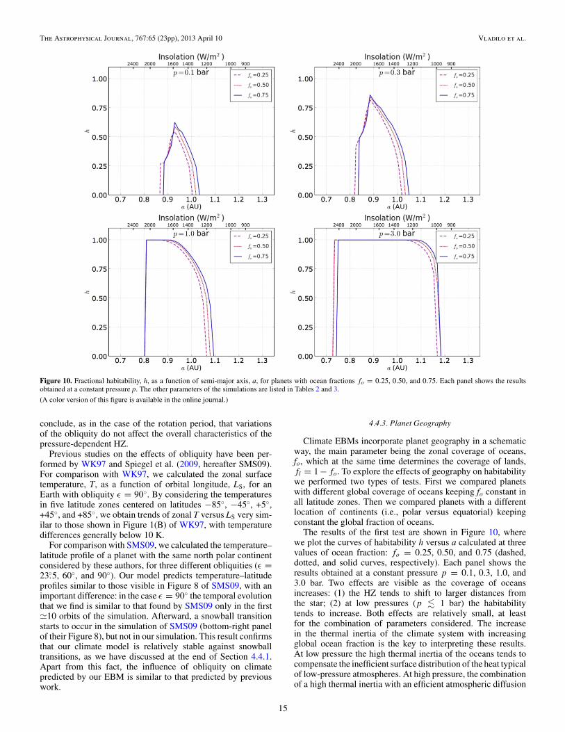
Figure 10. Fractional habitability, h, as a function of semi-major axis, a, for planets with ocean fractions fo = 0.25, 0.50, and 0.75. Each panel shows the resultsobtained at a constant pressure p. The other parameters of the simulations are listed in Tables 2 and 3.
(A color version of this figure is available in the online journal.)
conclude, as in the case of the rotation period, that variationsof the obliquity do not affect the overall characteristics of thepressure-dependent HZ.
Previous studies on the effects of obliquity have been per-formed by WK97 and Spiegel et al. (2009, hereafter SMS09).For comparison with WK97, we calculated the zonal surfacetemperature, T, as a function of orbital longitude, LS, for anEarth with obliquity ε = 90◦. By considering the temperaturesin five latitude zones centered on latitudes −85◦, −45◦, +5◦,+45◦, and +85◦, we obtain trends of zonal T versus LS very sim-ilar to those shown in Figure 1(B) of WK97, with temperaturedifferences generally below 10 K.
For comparison with SMS09, we calculated the temperature–latitude profile of a planet with the same north polar continentconsidered by these authors, for three different obliquities (ε =23.◦5, 60◦, and 90◦). Our model predicts temperature–latitudeprofiles similar to those visible in Figure 8 of SMS09, with animportant difference: in the case ε = 90◦ the temporal evolutionthat we find is similar to that found by SMS09 only in the first�10 orbits of the simulation. Afterward, a snowball transitionstarts to occur in the simulation of SMS09 (bottom-right panelof their Figure 8), but not in our simulation. This result confirmsthat our climate model is relatively stable against snowballtransitions, as we have discussed at the end of Section 4.4.1.Apart from this fact, the influence of obliquity on climatepredicted by our EBM is similar to that predicted by previouswork.
4.4.3. Planet Geography
Climate EBMs incorporate planet geography in a schematicway, the main parameter being the zonal coverage of oceans,fo, which at the same time determines the coverage of lands,fl = 1 −fo. To explore the effects of geography on habitabilitywe performed two types of tests. First we compared planetswith different global coverage of oceans keeping fo constant inall latitude zones. Then we compared planets with a differentlocation of continents (i.e., polar versus equatorial) keepingconstant the global fraction of oceans.
The results of the first test are shown in Figure 10, wherewe plot the curves of habitability h versus a calculated at threevalues of ocean fraction: fo = 0.25, 0.50, and 0.75 (dashed,dotted, and solid curves, respectively). Each panel shows theresults obtained at a constant pressure p = 0.1, 0.3, 1.0, and3.0 bar. Two effects are visible as the coverage of oceansincreases: (1) the HZ tends to shift to larger distances fromthe star; (2) at low pressures (p � 1 bar) the habitabilitytends to increase. Both effects are relatively small, at leastfor the combination of parameters considered. The increasein the thermal inertia of the climate system with increasingglobal ocean fraction is the key to interpreting these results.At low pressure the high thermal inertia of the oceans tends tocompensate the inefficient surface distribution of the heat typicalof low-pressure atmospheres. At high pressure, the combinationof a high thermal inertia with an efficient atmospheric diffusion
15
The Astrophysical Journal, 767:65 (23pp), 2013 April 10 Vladilo et al.
tends to give the same temperature at a somewhat smaller levelof insolation.
To investigate the effects of continental/ocean distribution,we considered the three model geographies proposed by WK97:(1) present-day Earth geography, (2) equatorial continent, and(3) polar continent. In practice, each model is specified by a setof ocean fractions, fo, of each latitude zone (Table III in WK97).The case (2) represents a continent located at latitudes |ϕ| < 20◦covering the full planet. The case (3) represents a polar continentat ϕ � −30◦. The global ocean coverage is approximately thesame (〈fo〉 � 0.7) in the three cases. As a result, we find thatthese different types of model geographies introduce modesteffects on the habitability curves. The habitability of present-day and equatorial continent geography are essentially identicalat all pressures. The polar continent geography is slightly lesshabitable. This is probably due to the combination of two factorsthat tend to form a larger ice cap in the presence of a polarcontinent: (1) ice on land has a higher albedo than ice on waterand (2) the thermal capacity of continents is lower than thatof oceans. In any case, the differences in habitability are smalland tend to disappear at p � 3 bar due to the fast rise of thehorizontal heat transport.
4.4.4. Albedo of the Continents
Albedo variations can shift the location of the HZ, movingthe HZ inward if the albedo increases, or outward if the albedodecreases. In our model, the albedos of the oceans, ice, andclouds are not free parameters since they are specified bywell-defined prescriptions (Appendix A.4). The albedo of thelands, al, is instead a free parameter. In the simulations run tobuild the map of Figure 3, we kept a fixed value al = 0.2,representative of the average of Earth continents. In a genericplanet, the albedo of lands can vary approximately between�0.1 and 0.35, depending on the type of surface. The lowestvalues are appropriate, for instance, for basaltic rocks or coniferforests, while the highest values for Sahara-like deserts orlimestone; Mars sand has �0.15, while grasslands have �0.2(Pierrehumbert 2010). Given this possible range of continentalalbedos, we have repeated our calculations for al = 0.1, 0.2,and 0.35. As a result, we find that the curve of habitability hversus a shifts closer to the star for al = 0.35 and away from thestar for al = 0.1. The maximum shift between the extreme casesis �0.03 AU. The shape of the habitability curves is virtuallyunaffected by these changes.
4.4.5. Surface Gradient of Latitudinal Heat Transport
With our formulation of the diffusion coefficient, we caninvestigate how planetary habitability is influenced by variationsof the heat transport efficiency. In practice, this can be done byvarying the parameter R, that represents the ratio between themaximum and minimum value of the diffusion coefficient inthe planet (Appendix A.2). The results shown in Figure 3 havebeen obtained for R = 6, a value optimized to match Earthexperimental data. We repeated our calculations for R = 3 andR = 12, keeping constant the fiducial value D0, that representsthe mean global efficiency of heat transport. As a result, we donot find any significant difference in planetary habitability eitherat high or low pressure. We conclude that the knowledge of theexact functional dependence on the latitude of the heat transportefficiency is not fundamental in predicting the properties of theHZ, at least with the simplified formalism adopted here thatdoes not consider the circulation due to atmospheric cells.
4.4.6. Summary
The main effects of varying planetary parameters can besummarized as follows. As far as the shape of the habitabilitycurves is concerned, the results at low pressure are quite sensitiveto variations of rotation period, axis obliquity, and oceancoverage. Specifically, the habitability tends to increase withincreasing rotation period, axis obliquity (up to ε � 60◦), andocean coverage. At high pressure, the shape of the habitabilitycurves becomes insensitive to variations of these parameters. Asfar as the location and radial extension of the habitability curvesis concerned, the results are modestly influenced by variationsof planetary parameters, even at low pressure. Variations of thelatitudinal/seasonal gradient of the heat transport efficiency donot affect the properties of the HZ. Albedo variations tend toshift the habitability curves without affecting their shape.
4.5. Final Considerations
4.5.1. The Edges of the Habitable Zone
Our calculations do not include the CO2 climate stabilizationmechanism considered in the classic HZ definition (Kastinget al. 1993). In principle, EBM models can be used to simulatethe carbonate–silicate cycle that drives this mechanism (WK97).However, this choice is not practical when running thousandsof simulations, as we do here, because the timescale of the CO2cycle is much larger than the timescale of convergence of thesimulations. In addition, modeling the carbonate–silicate cyclerequires ad hoc assumptions on the silicate weathering law andrate of CO2 production by volcanos. At the present time it is notclear whether an active volcanism and tectonics, the ingredientsrequired for the existence of the CO2 cycle, are common interrestrial planets. For planets that do have this cycle, the outeredge of the HZ would shift to larger values of semi-major axisthan estimated here. For completeness we note that, if oceansare salty, the outer edge would shift in the same direction due tothe lowering of the water freezing point.
As far as the inner edge is concerned, we adopt the water-losslimit criterion (3). At p = 1 bar, our inner edge is located ata = 0.82 AU, in the range of inner limits predicted by Selsiset al. (2007). However, the study of the latitude–temperatureprofiles obtained from our simulations shows the existence ofcases that challenge the definition of the inner edge. Specifically,at low values of a and p in Figure 3, we find planets that arehabitable, but have temperatures above the boiling point of waterin some latitude zones. An example is shown in the right panelof Figure 5. The water reservoir of these type of planets is likelyto undergo a complete evaporation in the long term. In fact, toavoid this fate, the continental distribution and axis obliquityshould “conspire” to keep the oceans outside the boiling zoneduring all the planet’s life. This in turn would require (1) along-term mechanism of stabilization of the rotation axis and(2) the absence of tectonics drifts that, sooner or later, wouldbuild up a geography prone to evaporation. If the water reservoiris lost after an initial period of habitability, these planets matchthe definition of “Class II” habitats proposed by Lammer et al.(2009): bodies that possess Earth-like conditions in the earlystages of evolution, but not in the long term. According toLammer’s scheme, Venus is a potential “Class II” object thatmay have lost its water by evaporation. In contrast with Venus,the planets that we find have a low boiling point, typical oflow pressure, and can evaporate at a relatively cold globaltemperature. By excluding these “cold evaporating planets”from the map of Figure 3, the low-pressure inner edge would
16
The Astrophysical Journal, 767:65 (23pp), 2013 April 10 Vladilo et al.
shift to larger values of semi-major axis (e.g., from 0.87 AU to0.93 AU at p = 0.1 bar).
4.5.2. Which Type of Life?
Even if the HZ of Figure 3 broadens with pressure, thetype of life that can be expected to exist at a given level ofpressure p � 1 bar may be quite different, depending onthe exact location of the planet in the plane (a, p). Indeed,most of the enlargement of the HZ at high pressures is due tothe increasing fraction of regions with high temperatures lyingabove the isothermal contour Tm = 60◦C (red curve in Figure 3).Taking terrestrial life as a reference, these regions would only behabitable by extremophilic organisms, specifically thermophilesand hyperthermophiles (see, e.g., Cavicchioli 2002). In fact, noterrestrial extremophile is known to exist above �110–120◦C,the record being shared by a few archea living in oceanichydrothermal vents (Pyrolobus fumarii, Methanopyrus kandleristrain 116, and Strain 121). On these grounds, it is debatablewhether forms of life may exist beyond the isothermal contourTm = 120◦C (black curve in Figure 3). If we are interestedin the distribution of mesophilic organisms, rather than inextremophiles, the HZ does not become larger with increasingpressure: for organisms adapted to a temperature within therange 0◦C � Tm � 60◦C, the HZ shifts to larger distances fromthe central star as the pressure increases (region between themagenta and red curves in Figure 3).
As discussed above, the surface temperature becomes quiteuniform when the pressure exceeds a few bars. The uniformity ofthe temperature at all latitudes and seasons means that habitableplanets with high pressure can only host surface life adapted to afine-tuned range of temperatures. As an example, the maximumtemperature excursion at p = 5 bar at the outer edge of theHZ is −12◦C � T � +5◦C. This type of situation typicalof high pressure is quite different from that of Earth, wherethe latitudinal and seasonal variations allow the presence of awide diversity of surface life adapted to different temperatures.At lower pressures, the temperature excursions tend to becomequite high allowing, in principle, an even broader gamut ofsurface life. In particular, terrestrial-type cryophilic organismswith optimal temperature T < −15◦C would find a propersurface habitat only at low pressure (p � 1 bar) in the outermostregions of the HZ. However, at very low pressure the overallhabitability severely decreases and becomes restricted to anarrow range of distances from the star.
5. CONCLUSIONS
We have implemented a one-dimensional EBM of planetaryclimate, based on the diffusion equation (1), aimed at exploringthe surface habitability of extrasolar planets. Starting from themodel prescriptions adopted in previous EBMs, our modelcontains new recipes for the diffusion coefficient, the outgoingIR flux, the albedo, the effective thermal capacity, and the iceand cloud cover. Our prescription for the diffusion coefficientintroduces in a natural way seasonal and latitudinal variationsin the efficiency of the heat transport. The formalisms adoptedfor the calculation of the albedo and effective thermal capacityare sufficiently general to be applied to planets with a varietyof surface conditions. The recipe for the ice cover allows theformation of permanent ice caps or belts. The model parametershave been fine-tuned in such a way so as to reproduce themean annual latitude profiles of the Earth temperature andalbedo (Figure 1), as well as the seasonal variability of thetemperature–latitude profiles (Figure 2).
As a first application of our model, we have investigated thehabitability of planets with Earth-like atmospheric composi-tion but different levels of surface pressure. The habitability isestimated on the basis of the pressure-dependent liquid watertemperature range, taking into account the seasonal and latitu-dinal variations of the surface temperature. By running a largenumber of climate simulations with our EBM we have estimatedthe mean global annual temperature, Tm, and habitability, h, asa function of semi-major axis, a, and surface pressure, p. In thisway, we have built up a habitability map (Figure 3) that rep-resents the pressure-dependent HZ for planets with Earth-likeatmospheres orbiting a solar-type star. The main results that wefind can be summarized as follows.
1. The radial extent of the HZ increases with pressure, fromΔa = 0.18 AU at p = 1/3 bar to Δa = 0.43 AU atp = 3 bar.
2. At a given value of semi-major axis a, or insolation,q = L�/(4 π a2), the mean temperature and habitabilitytend to rise with increasing pressure (Figure 4).
3. Remarkable differences in surface temperature and habit-ability exist between the low- and high-pressure regimes,mainly because the range bracketed by extreme surface tem-peratures decreases with increasing pressure (Figure 4).
4. At low pressures (p � 0.3 bar) the habitability is generallylow and varies with a. At high pressure (p � 1 bar), thehabitability is high and relatively constant inside the HZ.
5. In the temperature range suitable for terrestrial mesophilicorganisms (0◦C � Tm � 60◦C), the HZ moves away fromthe star as pressure increases, rather than becoming broader.
The characteristics of the pressure-dependent HZ result fromthe complex interaction of physical effects that become strongeras the surface pressure increases. The main ones are the intensityof the greenhouse effect (recalling that we keep the atmosphericcomposition fixed), the efficiency of latitudinal heat transport,and the broadening of the temperature range of liquid water. Theincrease of the greenhouse effect bends the contours of equalplanet temperature toward higher distances from the star as thepressure increases. The broadening of the liquid water rangebends the inner edge of the HZ closer to the star as pressureincreases. The rise of the latitudinal heat transport tends to yielduniform planet temperatures at high pressure.
The comparison of our boundaries of habitability with thelimits of the classic HZ around a Sun-like star yields thefollowing conclusions. Our inner edge, calculated for Earth-likepressure, cloudiness, and humidity, is located at a = 0.82 AU, inthe range of the inner limits predicted by Selsis et al. (2007). Ourouter edge, calculated for Earth-like atmospheric composition,lies at a = 1.08 AU, much closer to the star than the quotedouter limits of the classic HZ, which are estimated for CO2-richplanetary atmospheres (Kasting et al. 1993; Selsis et al. 2007).
Thanks to the EBM capability of exploring the latitudinal andseasonal variations of the surface temperature we have found thefollowing results.
1. The mean global planet temperature, Tm, is not a goodindicator of habitability at low pressure. As an example,we find planets that are habitable even if Tm is well belowthe water freezing point (left panel of Figure 5). This resulthighlights the need of solving the latitude profile to properlycharacterize planetary habitability.
2. Habitable planets with zonal temperatures above the waterboiling point may in principle exist (right panel of Figure 5).These cases are new candidate “Class II” habitats (Lammer
17
The Astrophysical Journal, 767:65 (23pp), 2013 April 10 Vladilo et al.
et al. 2009), i.e., bodies that become unsuitable to host lifeafter an initial period of habitability.
Our results, calculated for circular orbits, can be extendedto planets in Keplerian orbits with moderate eccentricity (e <0.5), provided one uses the effective circular semi-major axisaeff = a(1 − e2)1/4 as a proxy of a. At higher eccentricities,however, the extent of the HZ shrinks considerably (Figure 7).In principle, our results can also be applied to planets orbitingstars different from the Sun, provided one uses the insolationq = L�/(4πa2) rather than the semi-major axis. In practice,there are several reasons, discussed in Section 4.3.2, why thistype of generalization should be done with caution.
The potential effects on climate of physical quantities uncon-strained by observations is a reason of concern in the study ofexoplanets. Thanks to the flexibility of our EBM simulationswe have explored how the habitability, and its dependence onpressure, can be influenced by changes of rotation period, axisobliquity, planet geography, and surface albedo. We find thefollowing results.
1. The shapes of the curves of habitability h versus a aresensitive to variations of planetary parameters at lowpressure, but not at high pressure.
2. The general location and radial extension of the pressure-dependent HZ are modestly influenced by planetary param-eters.
In conclusion, climate EBMs offer a powerful tool to deter-mine the range of stellar, orbital, and planetary parameters thatsatisfy the liquid water criterion in exoplanets. The possibilityof investigating seasonal and latitudinal variations of the surfacetemperature offers a significant insight on the habitability andits long-term evolution, as well as on the possible type of lifethat might exist on the planetary surface. These type of studieswill help to optimize the selection of targets in future searchesfor biomarkers in extrasolar planets.
We acknowledge helpful conversations with Marco Fulle,Michele Maris, Pierluigi Monaco, and Salvatore Scarpato.Thanks to Jost von Hardenberg for help in recovering andanalyzing Earth climate data. We also thank Rodrigo Caballeroand Raymond Pierrehumbert for help on the use of theirclimate utilities. The comments and suggestions received froman anonymous referee have improved the presentation of thiswork. G.V. thanks Kerrie for her enduring support and help inthe English revision of the manuscript.
APPENDIX
MODEL PRESCRIPTIONS
We present the formalism adopted to model the physicalquantities C, D, I, A, and S that appear in the diffusionequation (1). General introductory remarks on these quantitiesare given in Section 2. Further details can be found in theliterature cited in the text.
A.1. Effective Thermal Capacity, C
The term C represents the thermal inertia of the atmosphericand surface layers that contribute to the surface energy budget.For a layer with density ρ, specific heat capacity cp, anddepth Δ, the effective thermal capacity is C = ρ cp Δ.In a planet with oceans, the surface oceanic layers mixedby the winds provide the main contribution to the thermal
inertia. A wind-mixed ocean layer with Δ = 50 m hasCml50 = 210 × 106 J m−2 K−1 (WK97). Also the contributionof the atmosphere can be expressed in terms of an equivalentmixed ocean layer. For the Earth atmosphere, the equivalentocean depth is 2.4 m (Pierrehumbert 2010), corresponding toCatm,◦ = 10.1×10⁶ J m−2 K−1. For other planetary atmospheresthe thermal inertia will scale as(
Catm
Catm,◦
)=
(cp
cp,◦
) (p
p◦
), (A1)
where cp and p are the specific heat capacity and total pressureof the atmosphere, respectively (Pierrehumbert 2010). The ef-fective heat capacity of the solid surface is generally negligible.As a representative value, a layer of rock or ice with Δ = 0.5 myields a contribution Csolid � 1 × 10⁶ J m−2 K−1. This term,even if small, is not negligible in planets without oceans and withvery thin atmospheres. On the basis of the above considerations,we adopt
Co = Cml50 + Catm
Cl = Csolid + Catm (A2)
for the thermal inertia of the atmosphere over oceans and lands,respectively. For ices not undergoing liquid–solid transition, weadopt Ci = Cl . In the temperature range 263 < T < 273, weadd an extra contribution to the thermal inertia of ice to take intoaccount the latent heat of phase transition. In practice, based onsimilar recipes adopted by North et al. (1983) and WK97, weadopt Ci = Cl + Cml50/5.
The mean effective thermal capacity of each latitude zone iscalculated using as weighting factors the coverage of oceans, fo,and continents, fl = 1 − fo. The expression that we use
C = fl[(1 − fi) Cl + fi Ci] + fo[(1 − fi)Co + fi Ci] (A3)
takes into account the ice coverage, fi, estimated as explained inAppendix A.6.
All together, our values of thermal capacity are very similarto those adopted by WK97 and SMS08, with the exception ofCatm,◦, which is about twice in our case. Attempts to use highervalues of the ocean capacity previously proposed by North et al.(1983) and representative of a 75 m deep wind-mixed oceanlayer, yield a worse match between the model predictions andthe Earth experimental data.
A.2. Diffusion Coefficient, D
The horizontal transport of heat on the planet surface is mainlydue to the general circulations and the related instabilities of theocean and the atmosphere, which are governed by many factors.The most relevant are the physical and chemical propertiesof the atmosphere and oceans, the presence of Coriolis forceinduced by the planet rotation, and the topography of theplanet surface. Since EBMs are zonally averaged, longitudinalvariations of the heat transport are not considered. Even so,it is extremely difficult to model all the factors that govern thelatitudinal transport. To keep low the computational cost, EBMsincorporate the efficiency of the transport into a single quantity,namely the diffusion coefficient D, even though representinglatitudinal heat transport by a diffusive term is, in itself, agross simplification. In previous EBM work, this term has beenparameterized using a scaling law that takes into account thedependence of the diffusion coefficient on the main physical
18
The Astrophysical Journal, 767:65 (23pp), 2013 April 10 Vladilo et al.
quantities involved in the latitudinal transport. The relationproposed by WK97,
(D
D◦
)=
(p
p◦
) (cp
cp,◦
) (m
m◦
)−2 (ΩΩ◦
)−2
, (A4)
gives D as a function of atmospheric pressure, p, specific heatcapacity, cp, mean molecular weight, m, and angular velocity ofplanet rotation, Ω. All these quantities are scaled with respectto the reference Earth values. A discussion of the physicsunderlying this relation can be found in WK97. A number ofrecent applications of EBM to exoplanet climates have adoptedthe same relation (SMS08; Dressing et al. 2010). We referto these papers for cautionary remarks regarding the limits ofvalidity of the scaling relation D ∝ Ω−2.
In our work, we address an intrinsic limitation of the aboveformulation, namely the fact that, once the planet parameters arespecified, D is constant in latitude and time. This approximationis too crude because Earth’s latitudinal transport is drivenby atmospheric convective cells characterized by a latitudinalpattern with seasonal variations. As a consequence, in realplanets the efficiency of the diffusion will vary in latitude andtime. Here we propose a formalism that introduces latitudinaland seasonal variations of D related to the stellar zenith distance.This formalism can be applied to a generic planet.
Most of the latitudinal heat transport is carried out by thecirculation that takes place in the atmospheric convective cells.On Earth, the most notable of these features are the two Hadleycells that depart from the intertropical convergence zone (ITCZ)and produce the net effect of a polarward transport. The positionof the Hadley cells shifts during the year, influenced by thesolar zenith distance. This is demonstrated by the seasonal shiftof the ITCZ, which moves to higher latitudes in the summerhemisphere. Since the Hadley cells yield the largest contributionto the latitudinal heat transport, we conclude that the maximumefficiency of this type of transport is larger when the zenithdistance Z� is smaller. Inspired by this behavior, and withoutmaking specific assumptions on the systems of atmospheric cellsthat may be present in a generic planet, we have introduced adependence of the diffusion coefficient on μ = cos Z�. Morespecifically, we assume that D scales with the mean diurnalvalue μ, derived from Equation (A23). From this equation andEquation (A25) one can see that μ depends on the latitude, ϕ, andthe obliquity of the axis of rotation, ε; it also depends on the timeof the year, t, which determines the seasonal value of δ� and λ�.Therefore, by assuming a dependence D = D(μ) we introduce,in practice, a dependence on ϕ, t and ε. To incorporate this effectin the EBM prescriptions, we adopt the following expression:
(D
D◦
)= ζε(ϕ, t)
(p
p◦
) (cp
cp,◦
) (m
m◦
)−2 (ΩΩ◦
)−2
, (A5)
where ζε(ϕ, t) is a modulating factor that scales linearly withμ. This factor is normalized in such a way that the mean globalannual value of D equals that given by the scaling law (A4).Thanks to this fact, we can make use of the previous studiesof the diffusion coefficient, as far as the dependence on p, cp,m, Ω is concerned, and of our own formalism, as far as thedependence on ϕ, t, and ε is concerned. We now show howthe modulating factor ζε(ϕ, t) can be expressed as a functionof a single parameter, R, that represents the ratio between themaximum and minimum values of the diffusion coefficient inthe planet.
A.2.1. The Modulating Factor ζ
To obtain an expression for the modulating factor, ζ , we usethe following defining conditions: (1) ζ scales linearly with μ;and (2) ζ is normalized in such a way that its mean global annualvalue is 〈ζε(ϕ, t)〉 = 1. The first condition translates into
ζε(ϕ, t) = c0 + c1 με(ϕ, t), (A6)
where c0 and c1 are two constants. The second conditionbecomes
〈ζε(ϕ, t)〉 = c0 + c1 〈με(ϕ, t)〉 = 1, (A7)
where
〈με(ϕ, t)〉 =∫ P
0 dt∫ +π/2−π/2 dϕ cos ϕμε(ϕ, t)∫ P
0 dt∫ +π/2−π/2 dϕ cos ϕ
. (A8)
To determine c0 and c1, we need an additional relationbetween these two constants. For this purpose, we follow anapproach similar to that of North et al. (1983), who adjustedthe diffusion coefficient to be three times as large at the equatoras it is at the poles. In the framework of our formulation, thiscondition would be expressed in the form R = 3, where
R = [ζε(ϕ, t)]max
[ζε(ϕ, t)]min(A9)
is the ratio between the maximum and minimum values of themodulation factor in any latitude zone and at any orbital phase.The above condition is equivalent to
R = c0 + c1 [με(ϕ, t)]max
c0 + c1 [με(ϕ, t)]min= c0 + c1 [με(ϕ, t)]max
c0, (A10)
where we have used the fact that [με(ϕ, t)]min = 0 since μ = 0in the zones where the star lies below the horizon during a periodof rotation. We treat R as an input parameter of the model usedto estimate c0 and c1. By combining Equations (A7) and (A10),it is easy to show that
c1 =(
[με(ϕ, t)]max
R − 1+ 〈με(ϕ, t)〉
)−1
(A11)
and
c0 = c1 × [με(ϕ, t)]max
R − 1. (A12)
The quantities [με(ϕ, t)]max and 〈με(ϕ, t)〉 are calculatedgiven the obliquity ε. To compute the double integral inEquation (A8) we use the expression of μ given inEquation (A23), with the condition μ = 0 when H � 0, i.e.,when the Sun is below the local horizon for a complete rotationof the planet.
A.2.2. Calibration of R
The parameter R was tuned to improve the match betweenthe observed and predicted temperature–latitude profile of Earth.The observed profile shows two features that are quite difficult toreproduce with a simple EBM. One is the almost flat temperatureprofile within the tropical belt, the other is the sharp temperaturedrop at latitude ϕ � −60◦ (Figures 1 and 2). By increasing Rwe are able to improve the match to both features. We obtain thebest results by adopting R = 6. The temperature profile that weobtain is flatter at the tropics than in previous work (Figure 1);
19
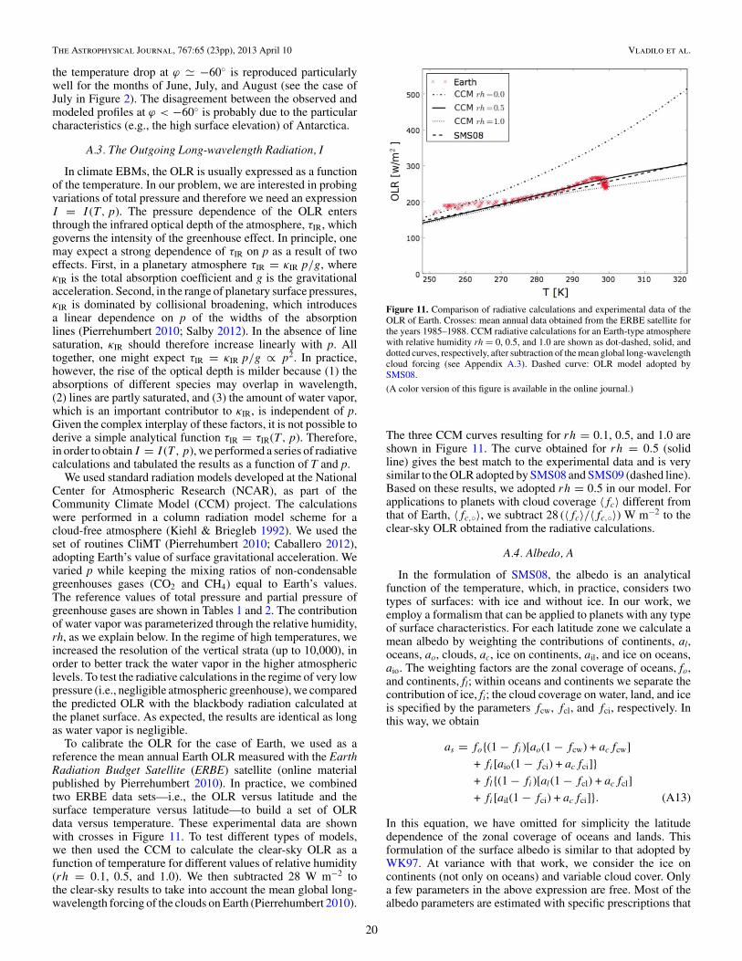
The Astrophysical Journal, 767:65 (23pp), 2013 April 10 Vladilo et al.
the temperature drop at ϕ � −60◦ is reproduced particularlywell for the months of June, July, and August (see the case ofJuly in Figure 2). The disagreement between the observed andmodeled profiles at ϕ < −60◦ is probably due to the particularcharacteristics (e.g., the high surface elevation) of Antarctica.
A.3. The Outgoing Long-wavelength Radiation, I
In climate EBMs, the OLR is usually expressed as a functionof the temperature. In our problem, we are interested in probingvariations of total pressure and therefore we need an expressionI = I (T , p). The pressure dependence of the OLR entersthrough the infrared optical depth of the atmosphere, τIR, whichgoverns the intensity of the greenhouse effect. In principle, onemay expect a strong dependence of τIR on p as a result of twoeffects. First, in a planetary atmosphere τIR = κIR p/g, whereκIR is the total absorption coefficient and g is the gravitationalacceleration. Second, in the range of planetary surface pressures,κIR is dominated by collisional broadening, which introducesa linear dependence on p of the widths of the absorptionlines (Pierrehumbert 2010; Salby 2012). In the absence of linesaturation, κIR should therefore increase linearly with p. Alltogether, one might expect τIR = κIR p/g ∝ p2. In practice,however, the rise of the optical depth is milder because (1) theabsorptions of different species may overlap in wavelength,(2) lines are partly saturated, and (3) the amount of water vapor,which is an important contributor to κIR, is independent of p.Given the complex interplay of these factors, it is not possible toderive a simple analytical function τIR = τIR(T , p). Therefore,in order to obtain I = I (T , p), we performed a series of radiativecalculations and tabulated the results as a function of T and p.
We used standard radiation models developed at the NationalCenter for Atmospheric Research (NCAR), as part of theCommunity Climate Model (CCM) project. The calculationswere performed in a column radiation model scheme for acloud-free atmosphere (Kiehl & Briegleb 1992). We used theset of routines CliMT (Pierrehumbert 2010; Caballero 2012),adopting Earth’s value of surface gravitational acceleration. Wevaried p while keeping the mixing ratios of non-condensablegreenhouses gases (CO2 and CH4) equal to Earth’s values.The reference values of total pressure and partial pressure ofgreenhouse gases are shown in Tables 1 and 2. The contributionof water vapor was parameterized through the relative humidity,rh, as we explain below. In the regime of high temperatures, weincreased the resolution of the vertical strata (up to 10,000), inorder to better track the water vapor in the higher atmosphericlevels. To test the radiative calculations in the regime of very lowpressure (i.e., negligible atmospheric greenhouse), we comparedthe predicted OLR with the blackbody radiation calculated atthe planet surface. As expected, the results are identical as longas water vapor is negligible.
To calibrate the OLR for the case of Earth, we used as areference the mean annual Earth OLR measured with the EarthRadiation Budget Satellite (ERBE) satellite (online materialpublished by Pierrehumbert 2010). In practice, we combinedtwo ERBE data sets—i.e., the OLR versus latitude and thesurface temperature versus latitude—to build a set of OLRdata versus temperature. These experimental data are shownwith crosses in Figure 11. To test different types of models,we then used the CCM to calculate the clear-sky OLR as afunction of temperature for different values of relative humidity(rh = 0.1, 0.5, and 1.0). We then subtracted 28 W m−2 tothe clear-sky results to take into account the mean global long-wavelength forcing of the clouds on Earth (Pierrehumbert 2010).
Figure 11. Comparison of radiative calculations and experimental data of theOLR of Earth. Crosses: mean annual data obtained from the ERBE satellite forthe years 1985–1988. CCM radiative calculations for an Earth-type atmospherewith relative humidity rh = 0, 0.5, and 1.0 are shown as dot-dashed, solid, anddotted curves, respectively, after subtraction of the mean global long-wavelengthcloud forcing (see Appendix A.3). Dashed curve: OLR model adopted bySMS08.
(A color version of this figure is available in the online journal.)
The three CCM curves resulting for rh = 0.1, 0.5, and 1.0 areshown in Figure 11. The curve obtained for rh = 0.5 (solidline) gives the best match to the experimental data and is verysimilar to the OLR adopted by SMS08 and SMS09 (dashed line).Based on these results, we adopted rh = 0.5 in our model. Forapplications to planets with cloud coverage 〈fc〉 different fromthat of Earth, 〈fc,◦〉, we subtract 28 (〈fc〉/〈fc,◦〉) W m−2 to theclear-sky OLR obtained from the radiative calculations.
A.4. Albedo, A
In the formulation of SMS08, the albedo is an analyticalfunction of the temperature, which, in practice, considers twotypes of surfaces: with ice and without ice. In our work, weemploy a formalism that can be applied to planets with any typeof surface characteristics. For each latitude zone we calculate amean albedo by weighting the contributions of continents, al,oceans, ao, clouds, ac, ice on continents, ail, and ice on oceans,aio. The weighting factors are the zonal coverage of oceans, fo,and continents, fl; within oceans and continents we separate thecontribution of ice, fi; the cloud coverage on water, land, and iceis specified by the parameters fcw, fcl, and fci, respectively. Inthis way, we obtain
as = fo{(1 − fi)[ao(1 − fcw) + acfcw]
+ fi[aio(1 − fci) + acfci]}+ fl{(1 − fi)[al(1 − fcl) + acfcl]
+ fi[ail(1 − fci) + acfci]}. (A13)
In this equation, we have omitted for simplicity the latitudedependence of the zonal coverage of oceans and lands. Thisformulation of the surface albedo is similar to that adopted byWK97. At variance with that work, we consider the ice oncontinents (not only on oceans) and variable cloud cover. Onlya few parameters in the above expression are free. Most of thealbedo parameters are estimated with specific prescriptions that
20
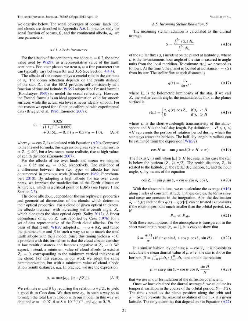
The Astrophysical Journal, 767:65 (23pp), 2013 April 10 Vladilo et al.
we describe below. The zonal coverages of oceans, lands, ice,and clouds are described in Appendix A.6. In practice, only thezonal fraction of oceans, fo, and the continental albedo, al, arefree parameters.
A.4.1. Albedo Parameters
For the albedo of the continents, we adopt al = 0.2, the samevalue used by WK97, as a representative value of the Earthcontinents. For other planets we treat al as a free parameter thatcan typically vary between 0.1 and 0.35 (see Section 4.4.4).
The albedo of the oceans plays a crucial role in the estimateof as. The ocean reflection depends on the zenith distanceof the star, Z�, that the EBM provides self-consistently as afunction of time and latitude. WK97 adopted the Fresnel formula(Kondratyev 1969) to model the ocean reflectivity. However,the Fresnel formula is an ideal approximation valid for smoothsurfaces while the actual sea level is never ideally smooth. Forthis reason we opted for a function calibrated with experimentaldata (Briegleb et al. 1986; Enomoto 2007):
ao = 0.026
(1.1 μ1.7 + 0.065)+ 0.15(μ − 0.1) (μ − 0.5) (μ − 1.0), (A14)
where μ = cos Z� is calculated with Equation (A20). Comparedto the Fresnel formula, this expression gives very similar resultsat Z� � 40◦, but a less steep, more realistic, rise at high valuesof zenith distance (Enomoto 2007).
For the albedo of ice over lands and ocean we adoptedail = 0.85 and aio = 0.62, respectively. The existence ofa difference between these two types of albedo has beendocumented in previous work (Kondratyev 1969; Pierrehum-bert 2010). By adopting a high albedo for ice over conti-nents, we improve the modelization of the Earth climate onAntarctica, which is a critical point of EBMs (see Figure 1 andSection 2.3).
The cloud albedo, ac, depends on the microphysical propertiesand geometrical dimensions of the clouds, which determinetheir optical properties. For a cloud of given optical thickness,the albedo increases with increasing stellar zenith angle, Z�,which elongates the slant optical depth (Salby 2012). A lineardependence of ac on Z� was reported by Cess (1976) for aset of data representative of the Earth cloud albedos. On thebasis of that result, WK97 adopted ac = α + βZ� and tunedthe parameters α and β in such a way so as to match the totalEarth albedo with their model. Since this tuning yields α < 0,a problem with this formalism is that the cloud albedo vanishesat low zenith distances and becomes negative at Z� = 0. Weexpect, instead, a minimum value of cloud albedo to exist atZ� = 0, corresponding to the minimum vertical thickness ofthe cloud. For this reason, in our work we adopt the sameparameterization, but with a minimum value of cloud albedoat low zenith distances, ac0. In practice, we use the expression
ac = max{ac0, [α + βZ�]}. (A15)
We estimate α and β by requiring the relation α + βZ� to yielda good fit to Cess data. We then tune ac0 in such a way so asto match the total Earth albedo with our model. In this way weobtained α = −0.07, β = 8 × 10⁻³(◦)−1, and ac0 = 0.19.
A.5. Incoming Stellar Radiation, S
The incoming stellar radiation is calculated as the diurnalaverage
S =∫ 2π
0 s(t�) dt�∫ 2π
0 dt�(A16)
of the stellar flux s(t�) incident on the planet at latitude ϕ, wheret� is the instantaneous hour angle of the star measured in angleunits from the local meridian. To estimate s(t�) we proceed asfollows. At the time t, the planet is located at a distance r = r(t)from its star. The stellar flux at such distance is
q(r) = L�
4πr2, (A17)
where L� is the bolometric luminosity of the star. If we callZ� the stellar zenith angle, the instantaneous flux at the planetsurface is
s(t�) ={τa q(r) cos Z� if|t�| < H0 if|t�| � H
(A18)
where τa is the short-wavelength transmissivity of the atmo-sphere and H is the half-day length. By definition, −H � t� �+H represents the portion of rotation period during which thestar stays above the horizon. The half-day length in radians canbe estimated from the expression (WK97)
cos H = − tan ϕ tan δ(0 < H < π ). (A19)
The flux s(t�) is null when |t�| � H because in this case the staris below the horizon (Z� � π/2). The zenith distance, Z�, isrelated to the latitude, ϕ, the stellar declination, δ�, and the hourangle, t�, by means of the equation
cos Z� = sin ϕ sin δ� + cos ϕ cos δ� cos t�. (A20)
With the above relations, we can calculate the average (A16)along circles of constant latitude. In these circles, the terms sin ϕand cos ϕ are constant in the integration. Also the declinationδ� = δ�(t) and the flux q(r) = q(r[t]) can be treated as constantsif the rotation period is much smaller than the orbital period, i.e.,if
Prot � Porb. (A21)
With these assumptions, if the atmosphere is transparent in theshort wavelength range (τa = 1), it is easy to show that
S = q(r)
π(H sin ϕ sin δ� + cos ϕ cos δ� sin H ) . (A22)
In a similar fashion, by defining μ = cos Z�, it is possible tocalculate the mean diurnal value of μ when the star is above thehorizon, μ = ∫ H
−Hμdt�/
∫ H
−Hdt�, and obtain the relation
μ = sin ϕ sin δ� + cos ϕ cos δ�
sin H
H(A23)
that we use in our formulation of the diffusion coefficient.Once we have obtained the diurnal average S, we calculate its
temporal variation in the course of the orbital period, S = S(t).The time t specifies the planet position along the orbit andS = S(t) represents the seasonal evolution of the flux at a givenlatitude. The only quantities that depend on t in Equation (A22)
21
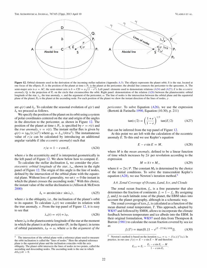
The Astrophysical Journal, 767:65 (23pp), 2013 April 10 Vladilo et al.
Figure 12. Orbital elements used in the derivation of the incoming stellar radiation (Appendix A.5). The ellipsis represents the planet orbit; S is the star, located atone focus of the ellipsis; Pt is the position of the planet at time t; P1 is the planet at the pericenter; the absidal line connects the pericenter to the apocenter, A. Thesemi-major axis is a = AC; the semi-minor axis is b = CD = a
√(1 − e2). Left panel: elements used to demonstrate relations (A24) and (A27); E is the eccentric
anomaly; Qt is the projection of Pt on the circle that circumscribes the orbit. Right panel: demonstration of the relation (A26) between the planetocentric orbitallongitude of the star, λ�, the true anomaly, ν, and the argument of the pericenter, ω. The line of nodes is the intersection between the orbital plane and the equatorialplane of the planet; P0 is the planet at the ascending node. For each position of the planet we show the instant direction of the lines of nodes, γ .
are q(r) and δ�. To calculate the seasonal evolution of q(r) andδ� we proceed as follows.
We specify the position of the planet on its orbit using a systemof polar coordinates centered on the star and origin of the anglesin the direction to the pericenter, as shown in Figure 12. Theposition of the planet at time t, Pt , is specified by r = r(t) andthe true anomaly, ν = ν(t). The instant stellar flux is given byq(r) = (q0/(r/a)2) where q0 = L�/(4πa2). The instantaneousvalue of r/a can be calculated by introducing an additionalangular variable E (the eccentric anomaly) such that
r/a = 1 − e cos E, (A24)
where e is the eccentricity and E is interpreted geometrically inthe left panel of Figure 12. We show below how to compute E.
To calculate the stellar declination δ� we consider the plan-etocentric orbital longitude of the star, λ�, shown in the rightpanel of Figure 12. The origin of this angle is the line of nodes,defined by the intersection of the orbital plane with the equato-rial plane. Without loss of generality, we set t = 0 the instant inwhich the planet crosses the ascending node.5 With this choice,the instant value of the stellar declination is (Allison & McEwen2000)
δ� = arcsin (sin ε sin λ�) , (A25)
where ε is the obliquity, i.e., the inclination of the planet’s orbitto its equator. To calculate λ�(t) we consider its relation withthe true anomaly, ν. From the top panel of Figure 12, it is easyto see that
λ�(t) = ν(t) + λP, (A26)
where λP is the planetocentric longitude of the star at the momentin which the planet is at the pericenter (P1 in the figure); in termsof orbital parameters, λP = ω, where ω is the argument of the
5 The intersection of the orbital plane with a reference plane used to measurethe orbit inclination is called the “lines of nodes.” Here the adopted referenceplane is the equatorial plane and the inclination coincides with the axisobliquity. The planet orbit intersects the lines of nodes in two points, called theascending and descending nodes. The ascending node is the one in whichd(δ�)/dt > 0.
pericenter. To solve Equation (A26), we use the expression(Bertotti & Farinella 1990, Equation (10.30), p. 211)
tan(ν/2) =(
1 + e
1 − e
)1/2
tan(E/2) (A27)
that can be inferred from the top panel of Figure 12.At this point we are left with the calculation of the eccentric
anomaly E. To this end we use Kepler’s equation
E − e sin E = M, (A28)
where M is the mean anomaly, defined to be a linear functionof time which increases by 2π per revolution according to theexpression
M = n t + M◦, (A29)
where n = 2π/P . The constant M0 is determined by the choiceof the initial conditions. To solve the transcendent Kepler’sequation (A28), we use Newton’s iteration method.6
A.6. Zonal Coverage of Oceans, Land, Ice, and Clouds
The zonal ocean fraction, fo, is a free parameter that alsodetermines the fraction of continents fl = 1 − fo. By assigningfo and fl to each latitude zone of the planet, the EBM takes intoaccount the planet geography, although in a schematic way.
The zonal coverage of ices, fi, is calculated as a function of themean diurnal zonal temperature, T. This approach, adopted byWK97 and followed by SM08, allows to incorporate the climatefeedback between temperature and ice albedo into the EBM. Intheir original formulation, WK97 used data from Thompson &Barron (1981) to calculate the ocean fraction covered by sea iceas
fi(T ) = max{0, [1 − e(T −273 K)/10 K]}. (A30)
6 Newton’s method is based on the iteration xi+1 = xi − f (xi )/f ′(xi ). Inpractice, in our case f (x) = E − e sin E − M and therefore
Ei+1 = Ei − Ei − e sin Ei − M
1 − e cos Ei
.
22
The Astrophysical Journal, 767:65 (23pp), 2013 April 10 Vladilo et al.
This expression provides a “freezing curve” that ideally de-scribes the formation of ices as the temperature decreases. How-ever, in this formulation the ice melts completely and instanta-neously as soon as T > 273 K. This approximation is too crudefor zones that are frozen for most of the time: in such regionswe expect a buildup of permanent ices if the timescales for iceformation and ice melting are comparable. To avoid this prob-lem, we compare the time intervals in which T < 273 K andT � 273 K in each zone. If T < 273 K during more than50% of the orbital period, we adopt a constant ice coveragefor the full orbit, fi = fi(T ), where T is the mean annualzonal temperature. In the other cases, we follow the originalformulation (A30). In this way we obtain the formation of per-manent ices, with a coverage that increases as the mean zonalannual temperature decreases. Our treatment significantly im-proves the description of the ice coverage on Earth, avoiding asudden appearance and disappearance of the polar caps in thecourse of each orbit. To keep the model simple, we adopt forthe continents the same ice coverage of the oceans. A morerealistic treatment of the ice coverage would require a formu-lation of the formation and melting of ices as a function oftime. The dynamical treatment of the ice formation and melt-ing is beyond the purpose of this paper and will be the sub-ject of subsequent work. We refer to Spiegel et al. (2010) fora detailed discussion of ice formation and melting using anEBM.
As far as the cloud coverage is concerned, we adopt differentvalues for clouds over oceans, continents, and ices in ourformulation of the albedo (Equation (A13)). The observationalsupport for variations of the cloud coverage on different typesof underlying surfaces comes from an analysis of Earth dataperformed by Sanroma & Palle (2012). These authors useddata collected by the International Satellite Cloud ClimatologyProject and presented the cloud coverage as a function of latitudefor clouds on water, ice, desert, and vegetation. We averagedthese latitude profiles to obtain a global representative cloudcoverage for each type of surface. The value for the water wasslightly adjusted to improve the agreement of our model withthe experimental albedo–latitude profiles of Earth. The cloudcoverage over continents was calculated by weighting desertsand vegetation with factors 2/3 and 1/3, respectively.7 As aresult, we adopt fcw = 0.67, fcl = 0.50, and fci = 0.50for clouds over water, continents, and ices, respectively. Withthis choice of parameters, we obtain a global cloud coverage〈fc〉 = 0.612 in our best model for Earth. This value is inagreement with the experimental value 〈fc〉 = 0.603 obtainedfrom the ERA Interim reanalysis for the years 1979–2010 (Deeet al. 2011). For comparison, WK97 adopted 〈fc〉 = 0.5 in theirformulation of the surface albedo of Earth. An interesting featureof our formalism is that the cloud coverage is automaticallyadjusted for planets with different fractions of continents,oceans, and ices.
REFERENCES
Allison, M., & McEwen, M. 2000, P&SS, 48, 215Anglada-Escude, G., Arriagada, P., Vogt, S. S., et al. 2012, ApJL,
751, L16
7 http://phl.upr.edu/library/notes/vegetationiceanddesertsofthepaleo-earth.
Bartik, K., Bruylants, G., Locci, E., & Reisse, J. 2011, in Origins and Evolutionof Life: An Astrobiological Perspective, ed. M. Gargaud, et al. (Cambridge:Cambridge Univ. Press), 205
Bertotti, B., & Farinella, P. 1990, Physics of the Earth and the Solar System(Dordrecht: Kluwer)
Borucki, W. J., Koch, D. G., Batalha, N., et al. 2012, ApJ, 745, 120Briegleb, B. P., Minnis, P., Ramanathan, V., & Harrison, E. 1986, JCAM,
25, 214Caballero, R. 2012, CliMT: An Object-oriented Climate Modeling and
Diagnostics Toolkit, http://people.su.se/∼rcaba/climtCavicchioli, R. 2002, AsBio, 2, 281Cess, R. D. 1976, JAtS, 33, 1831Dee, D. P., Uppala, S. M., Simmons, A. J., et al. 2011, QJRMS, 137, 553Dole, S. H. 1964, Habitable Planets for Man (New York: Blaisdell Pub. Co.)Dressing, C. D., Spiegel, D. S., Scharf, C. A., Menou, K., & Raymond, S. N.
2010, ApJ, 721, 1295Enomoto, T. 2007, JAMSTEC Report of Research and Development, 6, 21Forgan, D. 2012, MNRAS, 422, 1241Gaidos, E., & Williams, D. M. 2004, NewA, 10, 67Hart, M. H. 1979, Icar, 37, 351Heller, R., & Barnes, R. 2013, AsBio, 13, 18Heng, K., & Vogt, S. S. 2011, MNRAS, 415, 2145Howard, A. W., Marcy, G. W., Bryson, S. T., et al. 2012, ApJS, 201, 15Joshi, M. 2003, AsBio, 3, 415Kasting, J. F., & Catling, D. 2003, ARA&A, 41, 429Kasting, J. F., Whitmire, D. P., & Reynolds, R. T. 1993, Icar, 101, 108Kiehl, J. T., & Briegleb, B. P. 1992, JGR, 97, 10037Kite, E. S., Gaidos, E., & Manga, M. 2011, ApJ, 743, 41Kondratyev, K. Y. A. (ed.) 1969, Radiation in the Atmosphere (New York:
Academic)Kopp, G., & Lean, J. L. 2011, GeoRL, 38, L01706Lammer, H., Bredehoft, J. H., Coustenis, A., et al. 2009, A&ARv, 17, 181Latham, D. W., Rowe, J. F., Quinn, S. N., et al. 2011, ApJL, 732, L24Lide, D. R. 1997, CRC Handbook of Chemistry and Physics (Boca Raton, FL:
CRC Press)Lissauer, J. J., Ragozzine, D., Fabrycky, D. C., et al. 2011, ApJS, 197, 8Lo Curto, G., Mayor, M., Benz, W., et al. 2010, A&A, 512, A48Mayor, M., & Queloz, D. 1995, Natur, 378, 355McGuffie, K., & Henderson-Sellers, A. 2005, A Climate Modelling Primer (3rd
ed.; Chichester: Wiley)Mordasini, C., Alibert, Y., Benz, W., Klahr, H., & Henning, T. 2012, A&A,
541, 97North, G. R., & Coakley, J. A. 1979, JAtS, 36, 1189North, G. R., Mengel, J. G., & Short, D. A. 1983, JGR, 88, 6576Pepe, F., Lovis, C., Segransan, D., et al. 2011, A&A, 534, 58Pierrehumbert, R. T. 2010, Principles of Planetary Climate (Cambridge: Cam-
bridge Univ. Press)Pierrehumbert, R. T. 2011, ApJL, 726, L8Pierrehumbert, R. T., & Gaidos, E. 2011, ApJL, 734, L13Press, W. H., Flannery, B. P., Teukolsky, S. A., & Vetterling, W. T. 1992, Nu-
merical Recipes in Fortran 77: The Art of Scientific Computing (Cambridge:Cambridge Univ. Press)
Reynolds, R. T., McKay, C. P., & Kasting, J. F. 1987, AdSpR, 7, 125Salby, M. L. 2012, Physics of the Atmosphere and Climate (New York:
Cambridge Univ. Press)Sanroma, E., & Palle, E. 2012, ApJ, 744, 188Scharf, C. A. 2006, ApJ, 648, 1196Selsis, F., Kasting, J. F., Paillet, J., & Delfosse, X. 2007, A&A, 476, 1373Spiegel, D. S., Menou, K., & Scharf, C. A. 2008, ApJ, 681, 1609 (SMS08)Spiegel, D. S., Menou, K., & Scharf, C. A. 2009, ApJ, 691, 596 (SMS09)Spiegel, D. S., Raymond, S. N., Dressing, C. D., Scharf, C. A., & Mitchell,
J. L. 2010, ApJ, 721, 1308Thompson, S. L., & Barron, E. J. 1981, JG, 89, 143Tuomi, M., Anglada-Escude, G., Gerlach, E., et al. 2013, A&A, 549, 48Udry, S., & Santos, N. C. 2007, ARA&A, 45, 397Walker, J. C. G., Hays, P. B., & Kasting, J. F. 1981, JGR, 86, 9776Williams, D. M., & Kasting, J. F. 1997, Icar, 129, 254 (WK97)Williams, D. M., Kasting, J. F., & Wade, R. A. 1997, Natur, 385, 234Williams, D. M., & Pollard, D. 2002, IJAsB, 1, 61Wordsworth, R. D., Forget, F., Selsis, F., et al. 2011, ApJL, 733, L48
23