The Hubble Constant - Springer · 2019-08-13 · The Hubble Constant 7 that we understand their astrophysics well enough to work out what their luminosity or size actually is. Neither

Living Rev. Relativity, 18, (2015), 2DOI 10.1007/lrr-2015-2

The Hubble Constant

Neal JacksonJodrell Bank Centre for AstrophysicsSchool of Physics and Astronomy

University of ManchesterTuring Building

Manchester M13 9PL, U.K.email: [email protected]

http://www.jodrellbank.manchester.ac.uk/~njj/

Accepted: 14 August 2014Published: 24 September 2015

(Update of lrr-2007-4)

Abstract

I review the current state of determinations of the Hubble constant, which gives the lengthscale of the Universe by relating the expansion velocity of objects to their distance. There aretwo broad categories of measurements. The first uses individual astrophysical objects whichhave some property that allows their intrinsic luminosity or size to be determined, or allowsthe determination of their distance by geometric means. The second category comprises theuse of all-sky cosmic microwave background, or correlations between large samples of galaxies,to determine information about the geometry of the Universe and hence the Hubble constant,typically in a combination with other cosmological parameters. Many, but not all, object-based measurements give H 0 values of around 72 – 74 km s–1 Mpc–1, with typical errors of2 – 3 km s–1 Mpc–1. This is in mild discrepancy with CMB-based measurements, in particularthose from the Planck satellite, which give values of 67 – 68 km s–1 Mpc–1 and typical errors of1 – 2 km s–1 Mpc–1. The size of the remaining systematics indicate that accuracy rather thanprecision is the remaining problem in a good determination of the Hubble constant. Whethera discrepancy exists, and whether new physics is needed to resolve it, depends on detailsof the systematics of the object-based methods, and also on the assumptions about othercosmological parameters and which datasets are combined in the case of the all-sky methods.

Keywords: Cosmology, Hubble constant

© The Author(s). This article is distributed under aCreative Commons Attribution 4.0 International License.http://creativecommons.org/licenses/by/4.0/

http://dx.doi.org/10.1007/lrr-2015-2

http://www.jodrellbank.manchester.ac.uk/~njj/

http://www.livingreviews.org/lrr-2007-4

http://creativecommons.org/licenses/by/4.0/

Imprint / Terms of Use

Living Reviews in Relativity is a peer-reviewed open access journal published by the SpringerInternational Publishing AG, Gewerbestrasse 11, 6330 Cham, Switzerland. ISSN 1433-8351.

This article is distributed under the terms of the Creative Commons Attribution 4.0 InternationalLicense (http://creativecommons.org/licenses/by/4.0/), which permits unrestricted use, dis-tribution, and reproduction in any medium, provided you give appropriate credit to the originalauthor(s) and the source, provide a link to the Creative Commons license, and indicate if changeswere made. Figures that have been previously published elsewhere may not be reproduced withoutconsent of the original copyright holders.

Neal Jackson,“The Hubble Constant”,

Living Rev. Relativity, 18, (2015), 2.DOI 10.1007/lrr-2015-2.

http://creativecommons.org/licenses/by/4.0/

Article Revisions

Living Reviews supports two ways of keeping its articles up-to-date:

Fast-track revision. A fast-track revision provides the author with the opportunity to add shortnotices of current research results, trends and developments, or important publications tothe article. A fast-track revision is refereed by the responsible subject editor. If an articlehas undergone a fast-track revision, a summary of changes will be listed here.

Major update. A major update will include substantial changes and additions and is subject tofull external refereeing. It is published with a new publication number.

For detailed documentation of an article’s evolution, please refer to the history document of thearticle’s online version at http://dx.doi.org/10.1007/lrr-2015-2.

24 September 2014: Major revision, updated and expanded. The number of references hasincreased from 179 to 242.

A new section (2.1) on megamaser cosmography was added, as this has developed significantlysince the first edition.

Section 3 on the classical distance ladder has been extensively re-written. It now focuses muchless on the detailed disagreements based on the metallicity dependence of the P-L relationshipof Cepheids, since these have been superseded to a large extent by better calibration. Instead,more space is devoted to developments since 2007.

The gravitational-lensing section (2.2) has been extensively updated and much of the detailfrom pre-2007 papers has been removed in favour of discussion of developments since 2007,particularly the Suyu et al. papers and an update on the discussion of mass degeneracies.

The section on cosmological measurement (4) has been updated, mainly because of the adventof Planck since the first edition.

A new conclusion (5) has been added to try to tie together the results from different obser-vational programmes.

In addition, the order of the article has been extensively rearranged, following an updated intro-ductory section. A few sections (mostly where relatively little progress has been made) have beenchanged relatively little apart from correction of errors – i.e., the introduction and the sections onS-Z effect and gravitational waves.


Contents

1 Introduction 51.1 A brief history . . . . . . . . . . . . . . . . . . . . . . . . . . . . . . . . . . . . . . 51.2 A little cosmology . . . . . . . . . . . . . . . . . . . . . . . . . . . . . . . . . . . . 8

2 One-Step Distance Methods 112.1 Megamaser cosmology . . . . . . . . . . . . . . . . . . . . . . . . . . . . . . . . . . 112.2 Gravitational lenses . . . . . . . . . . . . . . . . . . . . . . . . . . . . . . . . . . . 12

2.2.1 Basics of lensing . . . . . . . . . . . . . . . . . . . . . . . . . . . . . . . . . 122.2.2 Principles of time delays . . . . . . . . . . . . . . . . . . . . . . . . . . . . . 132.2.3 The problem with lens time delays . . . . . . . . . . . . . . . . . . . . . . . 142.2.4 Time delay measurements . . . . . . . . . . . . . . . . . . . . . . . . . . . . 172.2.5 Derivation of H 0: Now, and the future . . . . . . . . . . . . . . . . . . . . . 17

2.3 The Sunyaev–Zel’dovich effect . . . . . . . . . . . . . . . . . . . . . . . . . . . . . . 192.4 Gamma-ray propagation . . . . . . . . . . . . . . . . . . . . . . . . . . . . . . . . . 21

3 Local Distance Ladder 223.1 Preliminary remarks . . . . . . . . . . . . . . . . . . . . . . . . . . . . . . . . . . . 223.2 Basic principle . . . . . . . . . . . . . . . . . . . . . . . . . . . . . . . . . . . . . . 223.3 Problems and comments . . . . . . . . . . . . . . . . . . . . . . . . . . . . . . . . . 25

3.3.1 Distance to the LMC . . . . . . . . . . . . . . . . . . . . . . . . . . . . . . . 253.3.2 Cepheid systematics . . . . . . . . . . . . . . . . . . . . . . . . . . . . . . . 253.3.3 SNe Ia systematics . . . . . . . . . . . . . . . . . . . . . . . . . . . . . . . . 273.3.4 Other methods of establishing the distance scale . . . . . . . . . . . . . . . 27

4 The CMB and Cosmological Estimates of the Distance Scale 294.1 The physics of the anisotropy spectrum and its implications . . . . . . . . . . . . . 294.2 Degeneracies and implications for H 0 . . . . . . . . . . . . . . . . . . . . . . . . . . 31

4.2.1 Combined constraints . . . . . . . . . . . . . . . . . . . . . . . . . . . . . . 32

5 Conclusion 34

References 36

List of Tables

1 Time delays, with 1-𝜎 errors, from the literature. . . . . . . . . . . . . . . . . . . . 182 Some recent measurements of 𝐻0 using the S-Z effect. . . . . . . . . . . . . . . . . 21

The Hubble Constant 5

1 Introduction

1.1 A brief history

The last century saw an expansion in our view of the world from a static, Galaxy-sized Universe,whose constituents were stars and “nebulae” of unknown but possibly stellar origin, to the viewthat the observable Universe is in a state of expansion from an initial singularity over ten billionyears ago, and contains approximately 100 billion galaxies. This paradigm shift was summarised ina famous debate between Shapley and Curtis in 1920; summaries of the views of each protagonistcan be found in [43] and [195].

The historical background to this change in world view has been extensively discussed andwhole books have been devoted to the subject of distance measurement in astronomy [176]. Atthe heart of the change was the conclusive proof that what we now know as external galaxies layat huge distances, much greater than those between objects in our own Galaxy. The earliest suchdistance determinations included those of the galaxies NGC 6822 [93], M33 [94] and M31 [96], byEdwin Hubble.

As well as determining distances, Hubble also considered redshifts of spectral lines in galaxyspectra which had previously been measured by Slipher in a series of papers [197, 198]. If a spectralline of emitted wavelength 𝜆0 is observed at a wavelength 𝜆, the redshift 𝑧 is defined as

𝑧 = 𝜆/𝜆0 − 1 . (1)

For nearby objects and assuming constant gravitational tidal field, the redshift may be thoughtof as corresponding to a recession velocity 𝑣 which for nearby objects behaves in a way predictedby a simple Doppler formula,1 𝑣 = 𝑐𝑧. Hubble showed that a relation existed between distanceand redshift (see Figure 1); more distant galaxies recede faster, an observation which can naturallybe explained if the Universe as a whole is expanding. The relation between the recession velocityand distance is linear in nearby objects, as it must be if the same dependence is to be observedfrom any other galaxy as it is from our own Galaxy (see Figure 2). The proportionality constantis the Hubble constant 𝐻0, where the subscript indicates a value as measured now. Unless theUniverse’s expansion does not accelerate or decelerate, the slope of the velocity–distance relation isdifferent for observers at different epochs of the Universe. As well as the velocity corresponding tothe universal expansion, a galaxy also has a “peculiar velocity”, typically of a few hundred kms–1,due to groups or clusters of galaxies in its vicinity. Peculiar velocities are a nuisance if determiningthe Hubble constant from relatively nearby objects for which they are comparable to the recessionvelocity. Once the distance is > 50 Mpc, the recession velocity is large enough for the error in 𝐻0

due to the peculiar velocity to be less than about 10%.Recession velocities are very easy to measure; all we need is an object with an emission line and

a spectrograph. Distances are very difficult. This is because in order to measure a distance, weneed a standard candle (an object whose luminosity is known) or a standard ruler (an object whoselength is known), and we then use apparent brightness or angular size to work out the distance.Good standard candles and standard rulers are in short supply because most such objects require

1 See [105] and references therein, e.g., [27], for discussion of the details of the interpretation of redshift in anexpanding Universe. The first level of sophistication involves maintaining the GR principle that space is locallyMinkowskian, so that in a small region of space all effects must reduce to SR (for instance, in Peacock’s [155]example, the expansion of the Universe does not imply that a long-lived human will grow to four metres tall inthe next 1010 years). Redshift can be thought of as a series of transformations in photon wavelengths between aninfinite succession of closely-separated observers, resulting in an overall wavelength shift between two observers witha finite separation and therefore an associated “velocity”. The second level of sophistication is to ask what thisvelocity actually represents. [105] calculates the ratio of photon wavelength shifts between pairs of fundamentalobservers to the shifts in their proper separation in the presence of arbitrary gravitational fields, and shows thatthis ratio only corresponds to the purely dynamical result if the gravitational tide is constant.

Living Reviews in RelativityDOI 10.1007/lrr-2015-2


6 Neal Jackson

Figure 1: Hubble’s original diagram of distance to nearby galaxies, derived from measurements usingCepheid variables, against velocity, derived from redshift. The Hubble constant is the slope of this relation,and in this diagram is a factor of nearly 10 steeper than currently accepted values. Image reproducedfrom [95].

Figure 2: Illustration of the Hubble law. Galaxies at all points of the square grid are receding from theblack galaxy at the centre, with velocities proportional to their distance away from it. From the point ofview of the second, green, galaxy two grid points to the left, all velocities are modified by vector additionof its velocity relative to the black galaxy (red arrows). When this is done, velocities of galaxies as seenby the second galaxy are indicated by green arrows; they all appear to recede from this galaxy, again witha Hubble-law linear dependence of velocity on distance.




that we understand their astrophysics well enough to work out what their luminosity or size actuallyis. Neither stars nor galaxies by themselves remotely approach the uniformity needed; even whenselected by other, easily measurable properties such as colour, they range over orders of magnitudein luminosity and size for reasons that are astrophysically interesting but frustrating for distancemeasurement. The ideal 𝐻0 object, in fact, is one which involves as little astrophysics as possible.

Hubble originally used a class of stars known as Cepheid variables for his distance determina-tions. These are giant blue stars, the best known of which is 𝛼UMa, or Polaris. In most normalstars, a self-regulating mechanism exists in which any tendency for the star to expand or contractis quickly damped out. In a small range of temperature on the Hertzsprung–Russell (H-R) dia-gram, around 7000 – 8000 K, particularly at high luminosity,2 this does not happen and pulsationsoccur. These pulsations, the defining property of Cepheids, have a characteristic form, a steep risefollowed by a gradual fall. They also have a period which is directly proportional to luminosity,because brighter stars are larger, and therefore take longer to pulsate. The period-luminosity re-lationship was discovered by Leavitt [123] by studying a sample of Cepheid variables in the LargeMagellanic Cloud (LMC). Because these stars were known to be all at the same distance, theircorrelation of apparent magnitude with period therefore implied the P-L relationship.

The Hubble constant was originally measured as 500 km s−1 Mpc−1 [95] and its subsequenthistory was a more-or-less uniform revision downwards. In the early days this was caused bybias3 in the original samples [12], confusion between bright stars and H ii regions in the originalsamples [97, 185] and differences between type I and II Cepheids4 [7]. In the second half of thelast century, the subject was dominated by a lengthy dispute between investigators favouringvalues around 50 km s−1 Mpc−1 and those preferring higher values of 100 km s−1 Mpc−1. Mostastronomers would now bet large amounts of money on the true value lying between these extremes,and this review is an attempt to explain why and also to try and evaluate the evidence for thebest-guess current value. It is not an attempt to review the global history of 𝐻0 determinations, asthis has been done many times, often by the original protagonists or their close collaborators. Foran overall review of this process see, for example, [223] and [210]. Compilations of data and analysisof them are given by Huchra (http://cfa-www.harvard.edu/~huchra/hubble), and Gott ([77],updated by [35]).5 Further reviews of the subject, with various different emphases and approaches,are given by [212, 68].

In summary, the ideal object for measuring the Hubble constant:

2 This is known in the literature as the “instability strip” and is almost, but not quite, parallel to the luminosityaxis on the H-R diagram. In normal stars, any compression of the star, and the associated rise in temperature,results in a decrease in opacity; the resulting escape of photons produces expansion and cooling. For stars in theinstability strip, a layer of partially ionized He close to the surface causes opacity to rise instead of falling with anincrease in temperature, producing a degree of positive feedback and consequently oscillations. The instability striphas a finite width, which causes a small degree of dispersion in period–luminosity correlations among Cepheids.

3 There are numerous subtle and less-subtle biases in distance measurement; see [213] for a blow-by-blow account.The simplest bias, the “classical” Malmquist bias, arises because, in any population of objects with a distributionin intrinsic luminosity, only the brighter members of the population will be seen at large distances. The result isthat the inferred average luminosity is greater than the true luminosity, biasing distance measurements towards thesystematically short. The Behr bias [12] from 1951 is a distance-dependent version of the Malmquist bias, namelythat at higher distances, increasingly bright galaxies will be missing from samples. This leads to an overestimate ofthe average brightness of the standard candle which becomes worse at higher distance.

4 Cepheids come in two flavours: type I and type II, corresponding to population I and II stars. Population II starsare an earlier metal-poor generation of stars, which formed after the hypothetical, truly primordial Population IIIstars, but before later-generation Population I stars like the Sun which contain significant extra amounts of elementsother than hydrogen and helium due to enrichment of the ISM by supernovae in the meantime. The name “Cepheid”derives from the fact that the star 𝛿 Cephei was the first to be identified (by Goodricke in 1784). Population IICepheids are sometimes known as W Virginis stars, after their prototype, W Vir, and a W Vir star is typically afactor of 3 fainter than a classical Cepheid of the same period.

5 The conclusion of the latter, that based on median statistics of the Huchra compilation, 𝐻0 = 67 ±2 km s−1 Mpc−1 , is slightly scary in retrospect given the Planck value of 67.2 ± 1.3 km s−1 Mpc−1 for a flatUniverse [2].


http://cfa-www.harvard.edu/~huchra/hubble


8 Neal Jackson

Has a property which allows it to be treated as either as a standard candle or as a standardruler

Can be used independently of other calibrations (i.e., in a one-step process)

Lies at a large enough distance (a few tens of Mpc or greater) that peculiar velocities aresmall compared to the recession velocity at that distance

Involves as little astrophysics as possible, so that the distance determination does not dependon internal properties of the object

Provides the Hubble constant independently of other cosmological parameters.

Many different methods are discussed in this review. We begin with one-step methods, andin particular with the use of megamasers in external galaxies – arguably the only method whichsatisfies all the above criteria. Two other one-step methods, gravitational lensing and Sunyaev–Zel’dovich measurements, which have significant contaminating astrophysical effects are also dis-cussed. The review then discusses two other programmes: first, the Cepheid-based distance lad-ders, where the astrophysics is probably now well understood after decades of effort, but whichare not one-step processes; and second, information from the CMB, an era where astrophysics isin the linear regime and therefore simpler, but where 𝐻0 is not determined independently of othercosmological parameters in a single experiment, without further assumptions.

1.2 A little cosmology

The expanding Universe is a consequence, although not the only possible consequence, of generalrelativity coupled with the assumption that space is homogeneous (that is, it has the same averagedensity of matter at all points at a given time) and isotropic (the same in all directions). In1922, Friedman [72] showed that given that assumption, we can use the Einstein field equations ofgeneral relativity to write down the dynamics of the Universe using the following two equations,now known as the Friedman equations:

2 − 1

3(8𝜋𝐺𝜌+ Λ)𝑎2 = −𝑘𝑐2, (2)

𝑎= −4

3𝜋𝐺(𝜌+ 3𝑝/𝑐2) +

1

3Λ . (3)

Here 𝑎 = 𝑎(𝑡) is the scale factor of the Universe. It is fundamentally related to redshift, becausethe quantity (1 + 𝑧) is the ratio of the scale of the Universe now to the scale of the Universe atthe time of emission of the light (𝑎0/𝑎). Λ is the cosmological constant, which appears in the fieldequation of general relativity as an extra term. It corresponds to a universal repulsion and wasoriginally introduced by Einstein to coerce the Universe into being static. On Hubble’s discoveryof the expansion of the Universe, he removed it, only for it to reappear seventy years later as aresult of new data [157, 169] (see also [34, 235] for a review). 𝑘 is a curvature term, and is −1,0, or +1, according to whether the global geometry of the Universe is negatively curved, spatiallyflat, or positively curved. 𝜌 is the density of the contents of the Universe, 𝑝 is the pressure anddots represent time derivatives. For any particular component of the Universe, we need to specifyan equation for the relation of pressure to density to solve these equations; for most componentsof interest such an equation is of the form 𝑝 = 𝑤𝜌. Component densities vary with scale factor 𝑎as the Universe expands, and hence vary with time.

At any given time, we can define a Hubble parameter

𝐻(𝑡) = /𝑎 , (4)




which is obviously related to the Hubble constant, because it is the ratio of an increase in scalefactor to the scale factor itself. In fact, the Hubble constant 𝐻0 is just the value of 𝐻 at the currenttime.6

If Λ = 0, we can derive the kinematics of the Universe quite simply from the first Friedmanequation. For a spatially flat Universe 𝑘 = 0, and we therefore have

𝜌 = 𝜌c ≡3𝐻2

8𝜋𝐺, (5)

where 𝜌c is known as the critical density. For Universes whose densities are less than this criticaldensity, 𝑘 < 0 and space is negatively curved. For such Universes it is easy to see from the firstFriedman equation that we require > 0, and therefore the Universe must carry on expandingfor ever. For positively curved Universes (𝑘 > 0), the right hand side is negative, and we reach apoint at which = 0. At this point the expansion will stop and thereafter go into reverse, leadingeventually to a Big Crunch as becomes larger and more negative.

For the global history of the Universe in models with a cosmological constant, however, weneed to consider the Λ term as providing an effective acceleration. If the cosmological constant ispositive, the Universe is almost bound to expand forever, unless the matter density is very muchgreater than the energy density in cosmological constant and can collapse the Universe before theacceleration takes over. (A negative cosmological constant will always cause recollapse, but is notpart of any currently likely world model). Carroll [34] provides further discussion of this point.

We can also introduce some dimensionless symbols for energy densities in the cosmologicalconstant at the current time, ΩΛ ≡ Λ/(3𝐻2

0 ), and in “curvature energy”, Ω𝑘 ≡ −𝑘𝑐2/𝐻20 . By

rearranging the first Friedman equation we obtain

𝐻2

𝐻20

=𝜌

𝜌c− Ω𝑘𝑎

−2 +ΩΛ . (6)

The density in a particular component of the Universe 𝑋, as a fraction of critical density, canbe written as

𝜌𝑋/𝜌c = Ω𝑋𝑎𝛼 , (7)

where the exponent 𝛼 represents the dilution of the component as the Universe expands. It isrelated to the 𝑤 parameter defined earlier by the equation 𝛼 = −3(1 + 𝑤). For ordinary matter𝛼 = −3, and for radiation 𝛼 = −4, because in addition to geometrical dilution as the universeexpands, the energy of radiation decreases as the wavelength increases. The cosmological constantenergy density remains the same no matter how the size of the Universe increases, hence for acosmological constant we have 𝛼 = 0 and 𝑤 = −1. 𝑤 = −1 is not the only possibility forproducing acceleration, however. Any general class of “quintessence” models for which 𝑤 < − 1

3will do; the case 𝑤 < −1 is probably the most extreme and eventually results in the acceleratingexpansion becoming so dominant that all gravitational interactions become impossible due to theshrinking boundary of the observable Universe, finally resulting in all matter being torn apart ina “Big Rip” [32]. In current models Λ will become increasingly dominant in the dynamics of theUniverse as it expands. Note that ∑

𝑋

Ω𝑋 +ΩΛ +Ω𝑘 = 1 (8)

by definition, because Ω𝑘 = 0 implies a flat Universe in which the total energy density in mattertogether with the cosmological constant is equal to the critical density. Universes for which Ω𝑘 is

6 Historically, the Hubble constant has often been quoted as 𝐻0 = 100ℎ km s−1 Mpc−1, as a way of maintainingagnosticism in an era where observations allowed a wide range in ℎ. This is largely disappearing, but papers usingℎ can be hard to interpret [42]



10 Neal Jackson

almost zero tend to evolve away from this point, so the observed near-flatness is a puzzle knownas the “flatness problem”; the hypothesis of a period of rapid expansion known as inflation in theearly history of the Universe predicts this near-flatness naturally. As well as a solution to theflatness problem, inflation is an attractive idea because it provides a natural explanation for thelarge-scale uniformity of the Universe in regions which would otherwise not be in causal contactwith each other.

We finally obtain an equation for the variation of the Hubble parameter with time in terms ofthe Hubble constant (see, e.g., [155]),

𝐻2 = 𝐻20 (ΩΛ +Ωm𝑎

−3 +Ωr𝑎−4 +Ω𝑘𝑎

−2) , (9)

where Ωr represents the energy density in radiation and Ωm the energy density in matter.To obtain cosmological distances, we need to perform integrals of the form

𝐷𝐶 = 𝑐

∫d𝑧

𝐻(𝑧), (10)

where the right-hand side can be expressed as a “Hubble distance” 𝐷𝐻 ≡ 𝑐/𝐻0, multiplied by anintegral over dimensionless quantities such as the Ω terms. We can define a number of distances incosmology, including the “comoving” distance 𝐷𝐶 defined above. The most important for presentpurposes are the angular diameter distance 𝐷A = 𝐷C/(1 + 𝑧), which relates the apparent angularsize of an object to its proper size, and the luminosity distance 𝐷L = (1+𝑧)2𝐷A, which relates theobserved flux of an object to its intrinsic luminosity. For currently popular models, the angulardiameter distance increases to a maximum as 𝑧 increases to a value of order 1, and decreasesthereafter. Formulae for, and fuller explanations of, both distances are given by [87].




2 One-Step Distance Methods

In this section, we examine the main methods for one-step Hubble constant determination usingastrophysical objects, together with their associated problems and assess the observational situationwith respect to each. Other methods have been proposed7 but do not yet have the observationsneeded to apply them.

2.1 Megamaser cosmology

To determine the Hubble constant, measurements of distance are needed. In the nearby universe,the ideal object is one which is distant enough for peculiar velocities to be small – in practicearound 50 Mpc – but for which a distance can be measured in one step and without a ladder ofcalibration involving other measurements in more nearby systems. Megamaser systems in externalgalaxies offer an opportunity to do this.

A megamaser system in a galaxy involves clumps of gas which are typically located ∼ 0.1 pcfrom the centre of the galaxy, close to the central supermassive black hole which is thought to lieat the centre of most if not all galaxies. These clumps radiate coherently in the water line at afrequency of approximately 22 GHz. This can be observed at the required milliarcsecond resolutionscale using Very Long Baseline Interferometry (VLBI) techniques. With VLBI spectroscopy, thevelocity of each individual clump can be measured accurately, and by repeated observations themovements of each clump can be followed and the acceleration determined. Assuming that theclumps are in Keplerian rotation, the radius of each clump from the central black hole can thereforebe calculated, and the distance to the galaxy follows from knowledge of this radius together withthe angular separation of the clump from the galaxy centre. The black-hole mass is also obtained asa by-product of the analysis. The analysis is not completely straightforward, as the disk is warpedand viscous, with four parameters (eccentricity, position angle, periapsis angle and inclination)describing the global properties of the disk and four further parameters describing the properties ofthe warping [100]. In principle it is vulnerable to systematics involving the modelling parametersnot adequately describing the disk, but such systematics can be simulated for plausible extradynamical components [100] and are likely to be small.

The first maser system to be discovered in an external galaxy was that in the object NGC 4258.This galaxy has a shell of masers which are oriented almost edge-on [136, 79] and apparentlyin Keplerian rotation. Measurements of the distance to this galaxy have become steadily moreaccurate since the original work [84, 98, 100], although the distance of ∼ 7 Mpc to this object isnot sufficient to avoid large (tens of percent) systematics due to peculiar velocities in any attemptto determine 𝐻0.

More recently, a systematic programme has been carried out to determine maser distancesto other, more distant galaxies; the Megamaser Cosmology Project [167]. The first fruits of thisprogramme include the measurement of the dynamics of the maser system in the galaxy UGC 3789,

7 For example, one topic that may merit more than a footnote in the future is the study of cosmology usinggravitational waves. In particular, a coalescing binary system consisting of two neutron stars produces gravitationalwaves, and under those circumstances the measurement of the amplitude and frequency of the waves determinesthe distance to the object independently of the stellar masses [193]. This was studied in more detail by [36] andextended to more massive black-hole systems [90, 45]. More massive coalescing signals produce lower-frequencygravitational-wave signals, which can be detected with the proposed LISA space-based interferometer (http://lisa.nasa.gov/documentation.html). The major difficulty is obtaining the redshift measurement to go with thedistance estimate, since the galaxy in which the coalescence event has taken place must be identified. Given this,however, the precision of the 𝐻0 measurement is limited only by weak gravitational lensing along the line of sight,and even this is reducible by observations of multiple systems or detailed investigations of matter along the line ofsight. 𝐻0 determinations to ∼ 2% should be possible, but depend on the launch of LISA or a similar mission. Thisis an event that is probably decades away, although a pathfinder mission to test some of the technology is due forlaunch in 2015.


http://lisa.nasa.gov/documentation.html

http://lisa.nasa.gov/documentation.html


12 Neal Jackson

which have become steadily more accurate as the campaign has progressed [167, 25, 168]. A distanceof 49.6±5.1 Mpc is determined, corresponding to 𝐻0 = 68.9±7.1 km s−1 Mpc−1 [168]; the error isdominated by the uncertainty in the likely peculiar velocity, which itself is derived from studies ofthe Tully–Fisher relation in nearby clusters [132]. Efforts are under way to find more megamasersto include in the sample, with success to date in the cases of NGC 6264 and Mrk 1419. Braatzet al. [24] and Kuo et al. [122] report preliminary results in the cases of the latter two objects,resulting in an overall determination of 𝐻0 = 68.0 ± 4.8 km s−1 Mpc−1 (68 ± 9 km s−1 Mpc−1

for NGC 6264). Tightening of the error bars as more megamasers are discovered, together withcareful modelling, are likely to allow this project to make the cleanest determination of the Hubbleconstant within the next five years.

2.2 Gravitational lenses

A general review of gravitational lensing is given by Wambsganss [233]; here we review the theorynecessary for an understanding of the use of lenses in determining the Hubble constant. Thisdetermination, like the megamaser method, is a one-step process, although at a much greaterdistance. It is thus interesting both as a complementary determination and as an opportunityto determine the Hubble parameter as a function of redshift. It has the drawback of possessingone serious systematic error associated with contaminating astrophysics, namely the detailed massmodel of the lens.

2.2.1 Basics of lensing

Light is bent by the action of a gravitational field. In the case where a galaxy lies close to the lineof sight to a background quasar, the quasar’s light may travel along several different paths to theobserver, resulting in more than one image.

The easiest way to visualise this is to begin with a zero-mass galaxy (which bends no lightrays) acting as the lens, and considering all possible light paths from the quasar to the observerwhich have a bend in the lens plane. From the observer’s point of view, we can connect all pathswhich take the same time to reach the observer with a contour in the lens plane, which in thiscase is circular in shape. The image will form at the centre of the diagram, surrounded by circlesrepresenting increasing light travel times. This is of course an application of Fermat’s principle;images form at stationary points in the Fermat surface, in this case at the Fermat minimum. Putless technically, the light has taken a straight-line path8 between the source and observer.

If we now allow the galaxy to have a steadily increasing mass, we introduce an extra time delay(known as the Shapiro delay) along light paths which pass through the lens plane close to thegalaxy centre. This makes a distortion in the Fermat surface (Figure 3). At first, its only effectis to displace the Fermat minimum away from the distortion. Eventually, however, the distortionbecomes big enough to produce a maximum at the position of the galaxy, together with a saddlepoint on the other side of the galaxy from the minimum. By Fermat’s principle, two further imageswill appear at these two stationary points in the Fermat surface. This is the basic three-image lensconfiguration, although in practice the central image at the Fermat maximum is highly demagnifiedand not usually seen.

If the lens is significantly elliptical and the lines of sight are well aligned, we can produce fiveimages, consisting of four images around a ring alternating between maxima and saddle points, anda central, highly demagnified Fermat maximum. Both four-image and two-image systems (“quads”and “doubles”) are in fact seen in practice. The major use of lens systems is for determining massdistributions in the lens galaxy, since the positions and fluxes of the images carry information aboutthe gravitational potential of the lens. Gravitational lensing has the advantage that its effects are

8 Strictly speaking, provided we ignore effects to do with curvature of the Universe.




independent of whether the matter is light or dark, so in principle the effects of both baryonic andnon-baryonic matter can be probed.

Figure 3: Illustration of a Fermat surface for a source (red symbol) close to the line of sight to a galaxy(green symbol). In each case the appearance of the images to the observer is shown by a greyscale, and thecontours of the Fermat surface are given by green contours. Note that images form at stationary points ofthe surface defined by the contours. In the three panels, the mass of the galaxy, and thus the distortionof the Fermat surface, increases, resulting in an increasingly visible secondary image at the position of thesaddle point. At the same time, the primary image moves further from the line of sight to the source. Ineach case the third image, at the position of the Fermat maximum, is too faint to see.

2.2.2 Principles of time delays

Refsdal [166] pointed out that if the background source is variable, it is possible to measure anabsolute distance within the system and therefore the Hubble constant. To see how this works,consider the light paths from the source to the observer corresponding to the individual lensedimages. Although each is at a stationary point in the Fermat time delay surface, the absolute lighttravel time for each will generally be different, with one of the Fermat minima having the smallesttravel time. Therefore, if the source brightens, this brightening will reach the observer at differenttimes corresponding to the two different light paths. Measurement of the time delay correspondsto measuring the difference in the light travel times, each of which is individually given by

𝜏 =𝐷l𝐷s

𝑐𝐷ls(1 + 𝑧l)

(1

2(𝜃 − 𝛽)2 − 𝜓(𝜃)

), (11)

where 𝛼, 𝛽 and 𝜃 are angles defined below in Figure 4, 𝐷l, 𝐷s and 𝐷ls are angular diameterdistances also defined in Figure 4, 𝑧l is the lens redshift, and 𝜓(𝜃) is a term representing theShapiro delay of light passing through a gravitational field. Fermat’s principle corresponds to therequirement that ∇𝜏 = 0. Once the differential time delays are known, we can then calculate theratio of angular diameter distances which appears in the above equation. If the source and lensredshifts are known, 𝐻0 follows from Eqs. 9 and 10. The value derived depends on the geometriccosmological parameters Ω𝑚 and ΩΛ, but this dependence is relatively weak. A handy rule ofthumb which can be derived from this equation for the case of a 2-image lens, if we make theassumption that the matter distribution is isothermal9 and 𝐻0 = 70 km s−1 Mpc−1, is

Δ𝜏 = (14 days)(1 + 𝑧l)𝐷

(𝑓 − 1

𝑓 + 1

)𝑠2, (12)

9 An isothermal model is one in which the projected surface mass density decreases as 1/𝑟. An isothermal galaxywill have a flat rotation curve, as is observed in many galaxies.



14 Neal Jackson

where 𝑧l is the lens redshift, 𝑠 is the separation of the images (approximately twice the Einsteinradius), 𝑓 > 1 is the ratio of the fluxes and 𝐷 is the value of 𝐷s𝐷l/𝐷ls in Gpc. A larger time delayimplies a correspondingly lower 𝐻0.

Figure 4: Basic geometry of a gravitational lens system. Image reproduced from [233]; copyright by theauthor.

The first gravitational lens was discovered in 1979 [232] and monitoring programmes began soonafterwards to determine the time delay. This turned out to be a long process involving a disputebetween proponents of a ∼ 400-day and a ∼ 550-day delay, and ended with a determination of417 ± 2 days [121, 189]. Since that time, over 20 more time delays have been determined (seeTable 1). In the early days, many of the time delays were measured at radio wavelengths byexamination of those systems in which a radio-loud quasar was the multiply imaged source (seeFigure 5). Recently, optically-measured delays have dominated, due to the fact that only a smalloptical telescope in a site with good seeing is needed for the photometric monitoring, whereas radiotime delays require large amounts of time on long-baseline interferometers which do not exist inlarge numbers.10 A time delay using 𝛾-rays has been determined for one lens [37] using correlatedvariations in a light-curve which contains emission from both images of the lens.

2.2.3 The problem with lens time delays

Unlike local distance determinations (and even unlike cosmological probes which typically usemore than one measurement), there is only one major systematic piece of astrophysics in thedetermination of 𝐻0 by lenses, but it is a very important one.11 This is the form of the potentialin Eq. (11). If one parametrises the potential in the form of a power law in projected mass density

10 Essentially all radio time delays have come from the VLA, although monitoring programmes with MERLINhave also been attempted.

11 The redshifts of the lens and source also need to be known, as does the position of the centre of the lens galaxy;this measurement is not always a trivial proposition [241].




T (MJD − 56100 days)80 90 100 110 120 130

Fγ (

10

−6 p

ho

ton

s c

m−

2s

−1)

0

2

4

6

8 1st flares

1st delay

Fermi ToO

2nd flares

2nd delay

Figure 5: The lens system JVAS B0218+357. Top right: the measurement of time delay of about10 days from asynchronous variations of the two lensed images [16]. The upper left panels show theHST/ACS image [241] on which can be seen the two images and the spiral lensing galaxy, and the radioMERLIN+VLA image [17] showing the two images together with an Einstein ring. The bottom panelshows the 𝛾-ray lightcurve [37], in which, although the components are not resolved, the sharpness of thevariations allows a time delay to be determined (at 11.46 ± 0.16 days, significantly greater than the radiotime delay). Image reproduced with permission from [37]; copyright by AAS.



16 Neal Jackson

versus radius, the index is −1 for an isothermal model. This index has a pretty direct degeneracy12

with the deduced length scale and therefore the Hubble constant; for a change of 0.1, the lengthscale changes by about 10%. The sense of the effect is that a steeper index, which correspondsto a more centrally concentrated mass distribution, decreases all the length scales and thereforeimplies a higher Hubble constant for a given time delay.

If an uncertainty in the slope of a power-law mass distribution were the only issue, then thiscould be constrained by lensing observables in the case where the source is extended, resultingin measurements of lensed structure at many different points in the lens plane [115]. This hasbeen done, for example, using multiple radio sources [38], VLBI radio structure [239] and in manyobjects using lensed structure of background galaxies [21], although in this latter case 𝐻0 is notmeasurable because the background objects are not variable. The degeneracy between the Hubbleconstant and the mass model is more general than this, however [76]. The reason is that lensingobservables give information about the derivatives of the Fermat surface; the positions of the imagesare determined by the first derivatives of the surface, and the fluxes by the second derivatives. Forany given set of lensing observables, we can move the intrinsic source position, thus changing theFermat surface, and then restore the observables to their original values by adjusting the massmodel and thus returning the Fermat surface to its original configuration. It therefore follows thatany given set of measurements of image positions and fluxes in a lens system is consistent with anumber of different mass models, and therefore a number of different values of 𝐻0, because thesource position cannot be determined. Therefore the assumption of a particular type of model,such as a power-law, itself constitutes a selection of a particular one out of a range of possiblemodels [192], each of which would give a different 𝐻0. Modelling degeneracies arise not only fromthe mass distribution within the lens galaxy, but also from matter along the line of sight. Theseoperate in the sense that, if a mass sheet is present which is not known about, the length scaleobtained is too short and consequently the derived value of 𝐻0 is too high.

There are a number of approaches to this mass-degeneracy problem. The first is to use anon-parametric model for the projected mass distribution, imposing only a minimum number ofphysically-motivated requirements such as monotonicity, and thereby generate large numbers ofmass models which are exactly consistent with the data. This was pioneered by Saha and Williamsin a series of papers [179, 237, 180, 177] in which pixellated models of galaxy mass distributionswere used. Although pixellated models are useful for exploring the space of allowed models, they donot break the essential degeneracy. Other priors may be used, however: in principle it should alsobe possible to reject some possible mass distributions on physical grounds, because we expect themass profiles to contain a central stellar cusp and a more extended dark matter halo. Undisturbeddark matter haloes should have profiles similar to a Navarro, Frenk & White (NFW, [139]) form,but they may be modified by adiabatic contraction during the process of baryonic infall when thegalaxy forms.

Second, it is possible to increase the reliability of individual lens mass models by gatheringextra information which partially breaks the mass degeneracy. A major improvement is availableby the use of stellar velocity dispersions [221, 220, 222, 119] measured in the lensing galaxy.As a standalone determinant of mass models in galaxies at 𝑧 ∼ 0.5, typical of lens galaxies, suchmeasurements are not very useful as they suffer from severe degeneracies with the structure of stellarorbits. However, the combination of lensing information (which gives a very accurate measurementof mass enclosed by the Einstein radius) and stellar dynamics (which gives, more or less, the massenclosed within the effective radius of the stellar light) gives a measurement that in effect selectsonly some of the family of possible lens models which fit a given set of lensing observables. The

12 As discussed extensively in [113, 117], this is not a global degeneracy, but arises because the lensed images tellyou about the mass distribution in the annulus centred on the galaxy and with inner and outer radii defined bythe inner and outer images. Kochanek [113] derives detailed expressions for the time delay in terms of the centralunderlying and controlling parameter, the surface density in this annulus [76].




method has large error bars, in part due to residual dependencies on the shape of stellar orbits,but also because these measurements are very difficult; each galaxy requires about one night ofgood seeing on a 10-m telescope. Nevertheless, this programme has the potential beneficial effectof reducing the dominant systematic error, despite the potential additional systematic from theassumptions about stellar orbits.

Third, we can remove problems associated with mass sheets associated with material extrinsicto the main lensing galaxy by measuring them using detailed studies of the environments of lensgalaxies. Studies of lens groups [60, 106, 59, 137] show that neglecting matter along the line of sighttypically has an effect of 10 – 20%, with matter close to the redshift of the lens contributing most.More recently, it has been shown that a combination of studies of number counts and redshifts ofnearby objects to the main lens galaxy, coupled with comparisons to large numerical simulationsof matter such as the Millenium Simulation, can reduce the errors associated with the environmentto around 3 – 4% [78].

2.2.4 Time delay measurements

Table 1 shows the currently measured time delays, with references and comments. The additionof new measurements is now occurring at a much faster rate, due to the advent of more system-atic dedicated monitoring programmes, in particular that of the COSMOGRAIL collaboration(e.g., [230, 231, 41, 164, 57]). Considerable patience is needed for these efforts in order to deter-mine an unambiguous delay for any given object, given the contaminating effects of microlensingand also the unavoidable gaps in the monitoring schedule (at least for optical monitoring pro-grammes) once per year as the objects move into the daytime. Derivation of time delays underthese circumstances is not a trivial matter, and algorithms which can cope with these effects havebeen under continuous development for decades [156, 114, 88, 217] culminating in a blind analysischallenge [50].

2.2.5 Derivation of H 0: Now, and the future

Initially, time delays were usually turned into Hubble constant values using assumptions about themass model – usually that of a single, isothermal power law [119] – and with rudimentary modellingof the environment of the lens system as necessary. Early analyses of this type resulted in ratherlow values of the Hubble constant [112] for some systems, sometimes due to the steepness of the lenspotential [221]. As the number of measured time delays expanded, combined analyses of multiplelens systems were conducted, often assuming parametric lens models [141] but also using MonteCarlo methods to account for quantities such as the presence of clusters around the main lens. Thesemethods typically give values around 70 km s−1 Mpc−1 – e.g., (68 ± 6 ± 8) km s−1 Mpc−1 fromOguri (2007) [141], but with an uncomfortably greater spread between lens systems than wouldbe expected on the basis of the formal errors. An alternative approach to composite modelling isto use non-parametric lens models, on the grounds that these may permit a wider range of massdistributions [177, 150] even though they also contain some level of prior assumptions. Saha etal. (2006) [177] used ten time-delay lenses for this purpose, and Paraficz et al. (2010) [150] extendedthe analysis to eighteen systems obtaining 66+6

−4 km s−1 Mpc−1, with a further extension by Sereno

& Paraficz (2014) [194] giving 66± 6± 4 (stat/syst) km s−1 Mpc−1.

In the last few years, concerted attempts have emerged to put together improved time-delayobservations with systematic modelling. For two existing time-delay lenses (CLASS B1608+656and RXJ 1131–1231) modelling has been undertaken [205, 206] using a combination of all ofthe previously described ingredients: stellar velocity dispersions to constrain the lens model andpartly break the mass degeneracy, multi-band HST imaging to evaluate and model the extendedlight distribution of the lensed object, comparison with numerical simulations to gauge the likely



18 Neal Jackson

Table 1: Time delays, with 1-𝜎 errors, from the literature. In some cases multiple delays have beenmeasured in 4-image lens systems, and in this case each delay is given separately for the two componentsin brackets. An additional time delay for CLASS B1422+231 [151] probably requires verification, and apublished time delay for Q0142–100 [120, 146] has large errors. Time delays for the CLASS and PKSobjects have been obtained using radio interferometers, and the remainder using optical telescopes.

Lens system Time delay Reference

[days]

CLASS 0218+357 10.5± 0.2 [16]

HE 0435-1-223 14.4+0.8−0.9 (AD) [116]

7.8± 0.8 (BC) also others [41]

SBS 0909+532 45+1−11 (2𝜎) [229]

RX 0911+0551 146± 4 [86]

FBQ 0951+2635 16± 2 [103]

Q 0957+561 417± 3 [121]

SDSS 1001+5027 119.3± 3.3 [164]

SDSS 1004+4112 38.4± 2.0 (AB) [65]

SDSS 1029+2623 [64]

HE 1104–185 161± 7 [140]

PG 1115+080 23.7± 3.4 (BC) [188]

9.4± 3.4 (AC)

RX 1131–1231 12.0+1.5−1.3 (AB) [138]

9.6+2.0−1.6 (AC)

87± 8 (AD)

[217]

SDSS J1206+4332 111.3± 3 [57]

SBS 1520+530 130± 3 [30]

CLASS 1600+434 51± 2 [28]

47+5−6 [118]

CLASS 1608+656 31.5+2−1 (AB) [61]

36+1−2 (BC)

77+2−1 (BD)

SDSS 1650+4251 49.5± 1.9 [230]

PKS 1830–211 26+4−5 [127]

WFI J2033–4723 35.5± 1.4 (AB) [231]

HE 2149–2745 103± 12 [29]

HS 2209+1914 20.0± 5 [57]

Q 2237+0305 2.7+0.5−0.9 h [44]




contribution of the line of sight to the lensing potential, and the performance of the analysisblind (without sight of the consequences for 𝐻0 of any decision taken during the modelling). Theresults of the two lenses together, 75.2+4.4

−4.2 and 73.1+2.4−3.6 km s−1 Mpc−1 in flat and open ΛCDM,

respectively, are probably the most reliable determinations of 𝐻0 from lensing to date, even if theydo not have the lowest formal error13.

In the immediate future, the most likely advances come from further analysis of existing timedelay lenses, although the process of obtaining the data for good quality time delays and constraintson the mass model is not a quick process. A number of further developments will expedite theprocess. The first is the likely discovery of lenses on an industrial scale using the Large SynopticSurvey Telescope (LSST, [101]) and the Euclid satellite [4], together with time delays producedby high cadence monitoring. The second is the availability in a few years’ time of > 8-m classoptical telescopes, which will ease the followup problem considerably. A third possibility whichhas been discussed in the past is the use of double source-plane lenses, in which two backgroundobjects, one of which is a quasar, are imaged by a single foreground object [74, 39]. Unfortunately,it appears [191] that even this additional set of constraints leave the mass degeneracy intact,although it remains to be seen whether dynamical information will help relatively more in theseobjects than in single-plane systems.

One potentially clean way to break mass model degeneracies is to discover a lensed type Iasupernova [142, 143]. The reason is that, as we have seen, the intrinsic brightness of SNe Ia canbe determined from their lightcurve, and it can be shown that the resulting absolute magnificationof the images can then be used to bypass the effective degeneracy between the Hubble constantand the radial mass slope. Oguri et al. [143] and also Bolton and Burles [20] discuss prospects forfinding such objects; future surveys with the Large Synoptic Survey Telescope (LSST) are likelyto uncover significant numbers of such events. The problem is likely to be the determination ofthe time delay, since nearly all such objects are subject to significant microlensing effects withinthe lensing galaxy which is likely to restrict the accuracy of the measurement [51].

2.3 The Sunyaev–Zel’dovich effect

The basic principle of the Sunyaev–Zel’dovich (S-Z) method [203], including its use to determinethe Hubble constant [196], is reviewed in detail in [18, 33]. It is based on the physics of hot (108 K)gas in clusters, which emits X-rays by bremsstrahlung emission with a surface brightness given bythe equation (see e.g., [18])

𝑏X =1

4𝜋(1 + 𝑧)3

∫𝑛2𝑒Λ𝑒 d𝑙 , (13)

where 𝑛𝑒 is the electron density and Λ𝑒 the spectral emissivity, which depends on the electrontemperature.

At the same time, the electrons of the hot gas in the cluster Compton upscatter photons fromthe CMB radiation. At radio frequencies below the peak of the Planck distribution, this causes a“hole” in radio emission as photons are removed from this spectral region and turned into higher-frequency photons (see Figure 6). The decrement is given by an optical-depth equation,

Δ𝐼(𝜈) = 𝐼0

∫𝑛𝑒𝜎𝑇Ψ(𝜈, 𝑇𝑒) d𝑙 , (14)

involving many of the same parameters and a function Ψ which depends on frequency and electrontemperature. It follows that, if both 𝑏X and Δ𝐼(𝑥) can be measured, we have two equations forthe variables 𝑛𝑒 and the integrated length 𝑙‖ through the cluster and can calculate both quantities.

13 The programme, known as H0LiCOW, is now continuing in order to measure time delays, improve models andderive further 𝐻0 values for more lenses.



20 Neal Jackson

Finally, if we assume that the projected size 𝑙⊥ of the cluster on the sky is equal to 𝑙‖, we canthen derive an angular diameter distance if we know the angular size of the cluster. The Hubbleconstant is then easy to calculate, given the redshift of the cluster.

Figure 6: S-Z decrement observation of Abell 697 with the Ryle telescope in contours superimposed onthe ROSAT image (grey-scale). Image reproduced with permission from [104]; copyright by RAS.

Although in principle a clean, single-step method, in practice there are a number of possibledifficulties. Firstly, the method involves two measurements, each with a list of possible errors.The X-ray determination carries a calibration uncertainty and an uncertainty due to absorptionby neutral hydrogen along the line of sight. The radio observation, as well as the calibration, issubject to possible errors due to subtraction of radio sources within the cluster which are unrelatedto the S-Z effect. Next, and probably most importantly, are the errors associated with the clustermodelling. In order to extract parameters such as electron temperature, we need to model thephysics of the X-ray cluster. This is not as difficult as it sounds, because X-ray spectral informationis usually available, and line ratio measurements give diagnostics of physical parameters. For thismodelling the cluster is usually assumed to be in hydrostatic equilibrium, or a “beta-model” (adependence of electron density with radius of the form 𝑛(𝑟) = 𝑛0(1 + 𝑟2/𝑟2c )

−3𝛽/2) is assumed.Several recent works [190, 22] relax this assumption, instead constraining the profile of the clusterwith available X-ray information, and the dependence of 𝐻0 on these details is often reassuringlysmall (< 10%). Finally, the cluster selection can be done carefully to avoid looking at prolateclusters along the long axis (for which 𝑙⊥ = 𝑙‖) and therefore seeing more X-rays than one wouldpredict. This can be done by avoiding clusters close to the flux limit of X-ray flux-limited samples,Reese et al. [165] estimate an overall random error budget of 20 – 30% for individual clusters. Asin the case of gravitational lenses, the problem then becomes the relatively trivial one of makingmore measurements, provided there are no unforeseen systematics.

The cluster samples of the most recent S-Z determinations (see Table 2) are not independent inthat different authors often observe the same clusters. The most recent work, that in [22] is largerthan the others and gives a higher𝐻0. It is worth noting, however, that if we draw subsamples fromthis work and compare the results with the other S-Z work, the 𝐻0 values from the subsamples are




Table 2: Some recent measurements of 𝐻0 using the S-Z effect. Model types are 𝛽 for the assumption ofa 𝛽-model and H for a hydrostatic equilibrium model. Some of the studies target the same clusters, withthree objects being common to more than one of the four smaller studies, The larger study [22] containsfour of the objects from [104] and two from [190].

Reference Number of clusters Model type 𝐻0 determination

[km s−1 Mpc−1]

[22] 38 𝛽 +H 76.9+3.9+10.0−3.4−8.0

[104] 5 𝛽 66+11+9−10−8

[228] 7 𝛽 67+30+15−18−6

[190] 3 H 69± 8

[131] 7 𝛽 66+14+15−11−15

[165] 18 𝛽 60+4+13−4−18

consistent. For example, the 𝐻0 derived from the data in [22] and modelling of the five clustersalso considered in [104] is actually lower than the value of 66 km s−1 Mpc−1 in [104]. Within thesmaller samples, the scatter is much lower than the quoted errors, partially due to the overlap insamples (three objects are common to more than one of the four smaller studies).

It therefore seems as though S-Z determinations of the Hubble constant are beginning to con-verge to a value of around 70 km s−1 Mpc−1, although the errors are still large, values in the lowto mid-sixties are still consistent with the data and it is possible that some objects may have beenobserved but not used to derive a published 𝐻0 value. Even more than in the case of gravitationallenses, measurements of 𝐻0 from individual clusters are occasionally discrepant by factors of nearlytwo in either direction, and it would probably teach us interesting astrophysics to investigate thesecases further.

2.4 Gamma-ray propagation

High-energy 𝛾-rays emitted by distant AGN are subject to interactions with ambient photonsduring their passage towards us, producing electron-positron pairs. The mean free path for thisprocess varies with photon energy, being smaller at higher energies, and is generally a substantialfraction of the distance to the sources. The observed spectrum of 𝛾-ray sources therefore shows ahigh-energy cutoff, whose characteristic energy decreases with increasing redshift. The expectedcutoff, and its dependence on redshift, has been detected with the Fermi satellite [1].

The details of this effect depend on the Hubble constant, and can therefore be used to measureit [183, 11]. Because it is an optical depth effect, knowledge of the interaction cross-section frombasic physics, together with the number density 𝑛𝑝 of the interacting photons, allows a length mea-surement and, assuming knowledge of the redshift of the source, 𝐻0. In practice, the cosmologicalworld model is also needed to determine 𝑛𝑝 from observables. From the existing Fermi data avalue of 72 km s−1 Mpc−1 is estimated [52] although the errors, dominated by the calculation ofthe evolution of the extragalactic background light using galaxy luminosity functions and spectralenergy distributions, are currently quite large (∼ 10 km s−1 Mpc−1).



22 Neal Jackson

3 Local Distance Ladder

3.1 Preliminary remarks

As we have seen, in principle a single object whose spectrum reveals its recession velocity, andwhose distance or luminosity is accurately known, gives a measurement of the Hubble constant.In practice, the object must be far enough away for the dominant contribution to the motion tobe the velocity associated with the general expansion of the Universe (the “Hubble flow”), as thisexpansion velocity increases linearly with distance whereas other nuisance velocities, arising fromgravitational interaction with nearby matter, do not. For nearby galaxies, motions associated withthe potential of the local environment are about 200 – 300 km s−1, requiring us to measure dis-tances corresponding to recession velocities of a few thousand km s−1 or greater. These recessionvelocities correspond to distances of at least a few tens of Mpc.

The Cepheid distance method, used since the original papers by Hubble, has therefore been tomeasure distances of nearby objects and use this knowledge to calibrate the brightness of moredistant objects compared to the nearby ones. This process must be repeated several times in orderto bootstrap one’s way out to tens of Mpc, and has been the subject of many reviews and books(see e.g., [176]). The process has a long and tortuous history, with many controversies and falseturnings, and which as a by-product included the discovery of a large amount of stellar astrophysics.The astrophysical content of the method is a disadvantage, because errors in our understandingpropagate directly into errors in the distance scale and consequently the Hubble constant. Thenumber of steps involved is also a disadvantage, as it allows opportunities for both random andsystematic errors to creep into the measurement. It is probably fair to say that some of theseerrors are still not universally agreed on. The range of recent estimates is in the low seventies ofkm s−1 Mpc−1, with the errors having shrunk by a factor of two in the last ten years, and thereasons for the disagreements (in many cases by different analysis of essentially the same data) areoften quite complex.

3.2 Basic principle

We first outline the method briefly, before discussing each stage in more detail. Nearby starshave a reliable distance measurement in the form of the parallax effect. This effect arises becausethe earth’s motion around the sun produces an apparent shift in the position of nearby starscompared to background stars at much greater distances. The shift has a period of a year, and anangular amplitude on the sky of the Earth-Sun distance divided by the distance to the star. Thedefinition of the parsec is the distance which gives a parallax of one arcsecond, and is equivalentto 3.26 light-years, or 3.09× 1016 m. The field of parallax measurement was revolutionised by theHipparcos satellite, which measured thousands of stellar parallax distances, including observationsof 223 Galactic Cepheids; of the Cepheids, 26 yielded determinations of reasonable significance [63].The Gaia satellite will increase these by a large factor, probably observing thousands of GalacticCepheids and giving accurate distances as well as colours and metallicities [225].

Some relatively nearby stars exist in clusters of a few hundred stars known as “open clusters”.These stars can be plotted on a Hertzsprung–Russell diagram of temperature, deduced from theircolour together with Wien’s law, against apparent luminosity. Such plots reveal a characteristicsequence, known as the “main sequence” which ranges from red, faint stars to blue, bright stars.This sequence corresponds to the main phase of stellar evolution which stars occupy for most oftheir lives when they are stably burning hydrogen. In some nearby clusters, notably the Hyades, wehave stars all at the same distance and for which parallax effects can give the absolute distance to<1% [159]. In such cases, the main sequence can be calibrated so that we can predict the absoluteluminosity of a main-sequence star of a given colour. Applying this to other clusters, a process




known as “main sequence fitting”, can also give the absolute distance to these other clusters; theerrors involved in this fitting process appear to be of the order of a few percent [5].

The next stage of the bootstrap process is to determine the distance to the nearest objectsoutside our own Galaxy, the Large and Small Magellanic Clouds. For this we can apply theopen-cluster method directly, by observing open clusters in the LMC. Alternatively, we can usecalibrators whose true luminosity we know, or can predict from their other properties. Suchcalibrators must be present in the LMC and also in open clusters (or must be close enough fortheir parallaxes to be directly measurable).

These calibrators include Mira variables, RR Lyrae stars and Cepheid variable stars, of whichCepheids are intrinsically the most luminous. All of these have variability periods which arecorrelated with their absolute luminosity (Section 1.1), and in principle the measurement of thedistance of a nearby object of any of these types can then be used to determine distances to moredistant similar objects simply by observing and comparing the variability periods.

The LMC lies at about 50 kpc, about three orders of magnitude less than that of the distantgalaxies of interest for the Hubble constant. However, one class of variable stars, Cepheid variables,can be seen in both the LMC and in galaxies at distances up to 20 – 30 Mpc. The coming of theHubble Space Telescope has been vital for this process, as only with the HST can Cepheids bereliably identified and measured in such galaxies.

Even the HST galaxies containing Cepheids are not sufficient to allow the measurement ofthe universal expansion, because they are not distant enough for the dominant velocity to be theHubble flow. The final stage is to use galaxies with distances measured with Cepheid variablesto calibrate other indicators which can be measured to cosmologically interesting distances. Themost promising indicator consists of type Ia supernovae (SNe), which are produced by binarysystems in which a giant star is dumping mass on to a white dwarf which has already gonethrough its evolutionary process and collapsed to an electron-degenerate remnant; at a criticalpoint, the rate and amount of mass dumping is sufficient to trigger a supernova explosion. Thephysics of the explosion, and hence the observed light-curve of the rise and slow fall, has the samecharacteristic regardless of distance. Although the absolute luminosity of the explosion is notconstant, type Ia supernovae have similar light-curves [163, 8, 209] and in particular there is a verygood correlation between the peak brightness and the degree of fading of the supernova 15 days14

after peak brightness (a quantity known as Δ𝑚15 [162, 82]). If SNe Ia can be detected in galaxieswith known Cepheid distances, this correlation can be calibrated and used to determine distancesto any other galaxy in which a SN Ia is detected. Because of the brightness of supernovae, theycan be observed at large distances and hence, finally, a comparison between redshift and distancewill give a value of the Hubble constant.

There are alternative indicators which can be used instead of SNe Ia for determination of 𝐻0; allof them rely on the correlation of some easily observable property of galaxies with their luminosityor size, thus allowing them to be used as standard candles or rulers respectively. For example, theedge-on rotation velocity 𝑣 of spiral galaxies scales with luminosity as 𝐿 ∝ 𝑣4, a scaling known asthe Tully–Fisher relation [224]. There is an equivalent for elliptical galaxies, known as the Faber–Jackson relation [58]. In practice, more complex combinations of observed properties are oftenused such as the 𝐷𝑛 parameter of [53] and [128], to generate measurable properties of ellipticalgalaxies which correlate well with luminosity, or the “fundamental plane” [53, 49] between threeproperties, the average surface brightness within an effective radius15 the effective radius 𝑟𝑒, andthe central stellar velocity dispersion 𝜎. Here we can measure surface brightnesses and 𝜎 and derivea standard ruler in terms of the true 𝑟𝑒 which can then be compared with the apparent size of thegalaxy.

14 Because of the expansion of the Universe, there is a time dilation of a factor (1 + 𝑧)−1 which must be appliedto timescales measured at cosmological distances before these are used for such comparisons.

15 The effective radius is the radius from within which half the galaxy’s light is emitted.



24 Neal Jackson

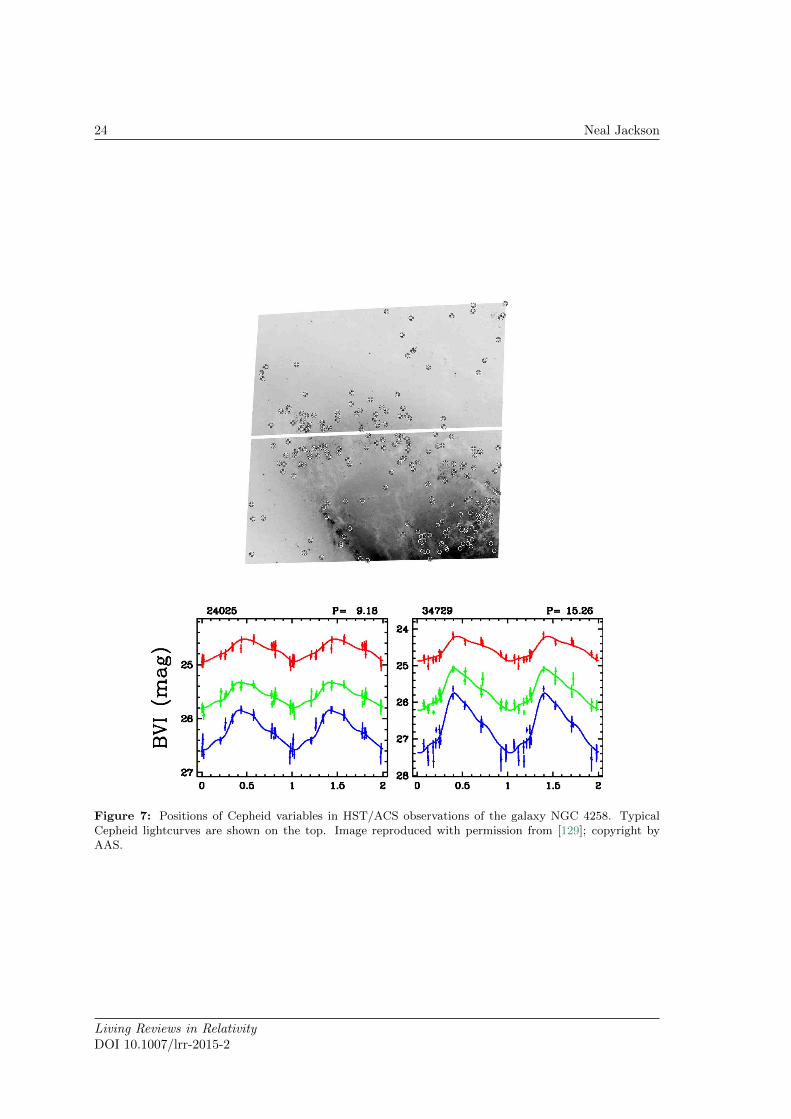
Figure 7: Positions of Cepheid variables in HST/ACS observations of the galaxy NGC 4258. TypicalCepheid lightcurves are shown on the top. Image reproduced with permission from [129]; copyright byAAS.




A somewhat different indicator relies on the fact that the degree to which stars within galaxiesare resolved depends on distance, in the sense that closer galaxies have more statistical “bumpiness”in the surface-brightness distribution [219] because of the degree to which Poisson fluctuations inthe stellar surface density are visible. This method of surface brightness fluctuation can also becalibrated by Cepheid variables in the nearer galaxies.

3.3 Problems and comments

3.3.1 Distance to the LMC

The LMC distance is probably the best-known, and least controversial, part of the distance ladder.Some methods of determination are summarised in [62]; independent calibrations using RR Lyraevariables, Cepheids and open clusters, are consistent with a distance of ∼ 50 kpc. An earlymeasurement, independent of all of the above, was made by [149] using the type II supernovaSN 1987A in the LMC. This supernova produced an expanding ring whose angular diameter couldbe measured using the HST. An absolute size for the ring could also be deduced by monitoringultraviolet emission lines in the ring and using light travel time arguments, and the distance of51.2 ± 3.1 kpc followed from comparison of the two. An extension to this light-echo method wasproposed in [200] which exploits the fact that the maximum in polarization in scattered light isobtained when the scattering angle is 90∘. Hence, if a supernova light echo were observed inpolarized light, its distance would be unambiguously calculated by comparing the light-echo timeand the angular radius of the polarized ring.

More traditional calibration methods traditionally resulted in distance moduli to the LMC of𝜇0 ≃ 18.50 (defined as 5 log 𝑑− 5, where 𝑑 is the distance in parsecs) corresponding to a distanceof ≃ 50 kpc. In particular, developments in the use of standard-candle stars, main sequencefitting and the details of SN 1987A are reviewed by [3] who concludes that 𝜇0 = 18.50 ± 0.02.This has recently been revised downwards slightly using a more direct calibration using parallaxmeasurements of Galactic Cepheids [14] to calibrate the zero-point of the Cepheid P-L relation inthe LMC [68]. A value of 𝜇0 = 18.40± 0.01 is found by these authors, corresponding to a distanceof 47.9± 0.2 kpc. The likely corresponding error in 𝐻0 is well below the level of systematic errorsin other parts of the distance ladder. This LMC distance also agrees well with the value neededin order to make the Cepheid distance to NGC 4258 agree with the maser distance ([129], see alsoSection 4).

3.3.2 Cepheid systematics

The details of the calibration of the Cepheid period-luminosity relation have historically caused themost difficulties in the local calibration of the Hubble constant. There are a number of minor effects,which can be estimated and calibrated relatively easy, and a dependence on metallicity which is asystematic problem upon which a lot of effort has been spent and which is now considerably betterunderstood.

One example of a minor difficulty is a selection bias in Cepheid programmes; faint Cepheids areharder to see. Combined with the correlation between luminosity and period, this means that onlythe brighter short-period Cepheids are seen, and therefore that the P-L relation in distant galaxiesis made artificially shallow [186] resulting in underestimates of distances. Neglect of this bias cangive differences of several percent in the answer, and detailed simulations of it have been carriedout by Teerikorpi and collaborators (e.g., [214, 152, 153, 154]). Most authors correct explicitlyfor this problem – for example, [71] calculate the correction analytically and find a maximum biasof about 3%. Teerikorpi & Paturel suggest that a residual bias may still be present, essentiallybecause the amplitude of variation introduces an additional scatter in brightness at a given period,in addition to the scatter in intrinsic luminosity. How big this bias is is hard to quantify, although



26 Neal Jackson

it can in principle be eliminated by using only long-period Cepheids at the cost of increases in therandom error.

The major systematic difficulty became apparent in studies of the biggest sample of Cepheidvariables, which arises from the OGLE microlensing survey of the LMC [227]. Samples of GalacticCepheids have been studied by many authors [62, 75, 67, 10, 13, 108], and their distances canbe calibrated by the methods previously described, or by using lunar-occultation measurementsof stellar angular diameters [66] together with stellar temperatures to determine distances byStefan’s law [236, 9]. Comparison of the P-L relations for Galactic and LMC Cepheids, however,show significant dissimilarities. In all three HST colours (𝐵, 𝑉 , 𝐼) the slope of the relations aredifferent, in the sense that Galactic Cepheids are brighter than LMC Cepheids at long periodsand are fainter at short periods. The two samples are of equal brightness in 𝐵 at a period ofapproximately 30 days, and at a period of a little more than 10 days in 𝐼.16

The culprit for this discrepancy is mainly metallicity17 differences in the Cepheids, which inturn results from the fact that the LMC is more metal-poor than the Galaxy. Unfortunately, manyof the external galaxies which are to be used for distance determination are likely to be similarin metallicity to the Galaxy, but the best local information on Cepheids for calibration purposescomes from the LMC. On average, the Galactic Cepheids tabulated by [81] are of approximatelyof solar metallicity, whereas those of the LMC are approximately 0.6 dex less metallic. If thesetwo samples are compared with their independently derived distances, a correlation of brightnesswith metallicity appears with a slope of −0.8± 0.3 mag dex−1 using only Galactic Cepheids, and−0.27 ± 0.08 mag dex−1 using both samples together. This can cause differences of 10 – 15% ininferred distance if the effect is ignored.

Many areas of historic disagreement can be traced back to how this correction is done. In partic-ular, two different 2005 – 2006 estimates of 73±4 (statistical) ±5 (systematic) km s−1 Mpc−1 [170]and 62.3± 1.3 (statistical) ±5 (systematic) km s−1 Mpc−1 [187], both based on the same Cepheidphotometry from the HST Key Project[178] and essentially the same Cepheid P-L relation for theLMC [218] have their origin mainly in this effect.18 One can apply a global correction for metallic-ity differences between the LMC and the galaxies in which the Cepheids are measured by the HSTKey Project [181], or attempt to interpolate between LMC and Galactic P-L relations [211] usinga period-dependent metallicity correction [187]. The differences in this correction account for the10 – 15% difference in the resulting value of 𝐻0.

More recently, a number of different solutions for this problem have been found, which aresummarised in the review by [68] and many of which involve getting rid of the intermediate LMCstep using other calibrations. [129] use ACS observations of Cepheids in the galaxy NGC 4258,which has a well-determined distance using maser observations (Section 4, [99, 80, 100]), and whoseCepheids have a range of metallicities[242]. Analysis of these Cepheids suggests that the use of aP-L relation whose slope varies with metallicity [211, 187] overcorrects at long period. Because ofthe known maser distance, these Cepheids can then be used both to determine the LMC distanceindependently [129] and also to calibrate the SNe distance scale and hence determine 𝐻0 [173, 172].The estimate has been incrementally improved by several methods in the last few years

Values obtained for the Hubble constant using the NGC 4258 calibration are quoted by [174]as 74.8± 3.1 km s−1 Mpc−1, using a value of 7.28 Mpc as the NGC 4258 distance. This was latercorrected by [100], who find a distance of 7.60 ± 0.17 (stat) ±0.15 (sys) Mpc using more VLBIepochs, together with better modelling of the masers, which therefore yields a Hubble constantof 72.0 ± 3.0 km s−1 Mpc−1. Efstathiou [54] has argued for further modifications, with different

16 Nearly all Cepheids measured in galaxies containing SN Ia have periods > 20 days, so the usual sense of theeffect is that Galactic Cepheids of a given period are brighter than LMC Cepheids.

17 Here, as elsewhere in astronomy, the term “metals” is used to refer to any element heavier than helium.Metallicity is usually quoted as 12+log(O/H), where O and H are the abundances of oxygen and hydrogen.

18 The details are discussed in more detail in an earlier version of this review [102].




criteria for rejecting outlying Cepheids; this lowers 𝐻0 to 70.6 ± 3.3 km s−1 Mpc−1. The alter-native distance ladder measurement, using parallax measurements of Galactic Cepheids [14] gives75.7 ± 2.6 km s−1 Mpc−1, and using the best available sample of LMC Cepheids observed in theinfrared [160] yields 74.4 ± 2.5 km s−1 Mpc−1. Infrared observations are important because theyreduce the potential error involved in extinction corrections. Indeed, the Carnegie Hubble Pro-gramme [69] takes this further by using mid-IR observations (at 3.6 𝜇m) of the Benedict et al.Galactic Cepheids with measured parallaxes, thus anchoring the calibration of the mid-IR P-Lrelation in these objects, and obtaining 𝐻0 = 74.3± 2.1 km s−1 Mpc−1. In the mid-IR, as well assmaller extinction corrections, metallicity effects are also generally less. However, arguments forlower values based on different outlier rejection can give a combined estimate for the three differentcalibrations [54] of 72.5± 2.5 km s−1 Mpc−1.

3.3.3 SNe Ia systematics

The calibration of the type Ia supernova distance scale, and hence 𝐻0, is affected by the selectionof galaxies used which contain both Cepheids and historical supernovae. Riess et al. [170] make thecase for the exclusion of a number of older supernovae from previous samples with measurementson photographic plates. Their exclusion, leaving four calibrators with data judged to be of highquality, has the effect of shrinking the average distances, and hence raising 𝐻0, by a few percent.Freedman et al. [71] included six galaxies including SN 1937C, excluded by [170], but obtainedapproximately the same value for 𝐻0.

Since SNe Ia occur in galaxies, their brightnesses are likely to be altered by extinction in thehost galaxy. This effect can be assessed and, if necessary, corrected for, using information aboutSNe Ia colours in local SNe. The effect is found to be smaller than other systematics within thedistance ladder [172].

Further possible effects include differences in SNe Ia luminosities as a function of environment.Wang et al. [234] used a sample of 109 supernovae to determine a possible effect of metallicityon SNe Ia luminosity, in the sense that supernovae closer to the centre of the galaxy (and henceof higher metallicity) are brighter. They include colour information using the indicator Δ𝐶12 ≡(𝐵 − 𝑉 )12 days, the 𝐵 − 𝑉 colour at 12 days after maximum, as a means of reducing scatter inthe relation between peak luminosity and Δ𝑚15 which forms the traditional standard candle.Their value of 𝐻0 is, however, quite close to the Key Project value, as they use the four galaxiesof [170] to tie the supernova and Cepheid scales together. This closeness indicates that the SNe Iaenvironment dependence is probably a small effect compared with the systematics associated withCepheid metallicity.

3.3.4 Other methods of establishing the distance scale

In some cases, independent distances to galaxies are available in the form of studies of the tipof the red giant branch. This phenomenon refers to the fact that metal-poor, population II redgiant stars have a well-defined cutoff in luminosity which, in the 𝐼-band, does not vary muchwith nuisance parameters such as stellar population age. Deep imaging can therefore provide anindependent standard candle which can be compared with that of the Cepheids, and in particularwith the metallicity of the Cepheids in different galaxies. The result [181] is again that metal-richCepheids are brighter, with a quoted slope of −0.24 ± 0.05 mag dex−1. This agrees with earlierdeterminations [111, 107] and is usually adopted when a global correction is applied.

Several different methods have been proposed to bypass some of the early rungs of the distancescale and provide direct measurements of distance to relatively nearby galaxies. Many of these arereviewed in the article by Olling [144].

One of the most promising methods is the use of detached eclipsing binary stars to determinedistances directly [147]. In nearby binary stars, where the components can be resolved, the de-



28 Neal Jackson

termination of the angular separation, period and radial velocity amplitude immediately yields adistance estimate. In more distant eclipsing binaries in other galaxies, the angular separation can-not be measured directly. However, the light-curve shapes provide information about the orbitalperiod, the ratio of the radius of each star to the orbital separation, and the ratio of the stars’luminosities. Radial velocity curves can then be used to derive the stellar radii directly. If we canobtain a physical handle on the stellar surface brightness (e.g., by study of the spectral lines) thenthis, together with knowledge of the stellar radius and of the observed flux received from each star,gives a determination of distance. The DIRECT project [23] has used this method to derive adistance of 964±54 kpc to M33, which is higher than standard distances of 800 – 850 kpc [70, 124].It will be interesting to see whether this discrepancy continues after further investigation.

A somewhat related method, but involving rotations of stars around the centre of a distantgalaxy, is the method of rotational parallax [161, 145, 144]. Here one observes both the propermotion corresponding to circular rotation, and the radial velocity, of stars within the galaxy.Accurate measurement of the proper motion is difficult and will require observations from futurespace missions.




4 The CMB and Cosmological Estimates of the DistanceScale

4.1 The physics of the anisotropy spectrum and its implications

The physics of stellar distance calibrators is very complicated, because it comes from the era inwhich the Universe has had time to evolve complicated astrophysics. A large class of alternativeapproaches to cosmological parameters in general involve going back to an era where astrophysicsis relatively simple and linear, the epoch of recombination at which the CMB fluctuations canbe studied. Although tests involving the CMB do not directly determine 𝐻0, they provide jointinformation about 𝐻0 and other cosmological parameters which is improving at a very rapid rate.

In the Universe’s early history, its temperature was high enough to prohibit the formation ofatoms, and the Universe was therefore ionized. Approximately 4 × 105 yr after the Big Bang,corresponding to a redshift 𝑧rec ∼ 1000, the temperature dropped enough to allow the formationof atoms, a point known as “recombination”. For photons, the consequence of recombination wasthat photons no longer scattered from ionized particles but were free to stream. After recombina-tion, these primordial photons reddened with the expansion of the Universe, forming the cosmicmicrowave background (CMB) which we observe today as a black-body radiation background at2.73 K.

In the early Universe, structure existed in the form of small density fluctuations (𝛿𝜌/𝜌 ∼ 0.01)in the photon-baryon fluid. The resulting pressure gradients, together with gravitational restoringforces, drove oscillations, very similar to the acoustic oscillations commonly known as sound waves.Fluctuations prior to recombination could propagate at the relativistic (𝑐/

√3) sound speed as the

Universe expanded. At recombination, the structure was dominated by those oscillation frequencieswhich had completed a half-integral number of oscillations within the characteristic size of theUniverse at recombination;19 this pattern became frozen into the photon field which formed theCMB once the photons and baryons decoupled and the sound speed dropped. The process isreviewed in much more detail in [92].

The resulting “acoustic peaks” dominate the fluctuation spectrum (see Figure 8). Their angularscale is a function of the size of the Universe at the time of recombination, and the angular diame-ter distance between us and 𝑧rec. Since the angular diameter distance is a function of cosmologicalparameters, measurement of the positions of the acoustic peaks provides a constraint on cosmo-logical parameters. Specifically, the more closed the spatial geometry of the Universe, the smallerthe angular diameter distance for a given redshift, and the larger the characteristic scale of theacoustic peaks. The measurement of the peak position has become a strong constraint in successiveobservations (in particular BOOMERanG [47], MAXIMA [83], and WMAP, reported in [201] and[202]) and corresponds to an approximately spatially flat Universe in which Ωm +ΩΛ ≃ 1.

But the global geometry of the Universe is not the only property which can be deduced from thefluctuation spectrum.20 The peaks are also sensitive to the density of baryons, of total (baryonic+ dark) matter, and of vacuum energy (energy associated with the cosmological constant). Thesedensities scale with the square of the Hubble parameter times the corresponding dimensionlessdensities [see Eq. (5)] and measurement of the acoustic peaks therefore provides information onthe Hubble constant, degenerate with other parameters, principally Ωm and ΩΛ. The second peakstrongly constrains the baryon density, Ωb𝐻

20 , and the third peak is sensitive to the total matter

density in the form Ωm𝐻20 .

19 This characteristic size is about 4 × 105 light years at recombination, corresponding to an angular scale ofabout 1∘ on the sky. The fact that the CMB is homogeneous on scales much larger than this is an illustration ofthe “horizon problem” discussed in Section 1.2, and which inflation may solve.

20 See http://background.uchicago.edu/~whu/intermediate/intermediate.html for a much longer expositionand tutorial on all these areas.


http://background.uchicago.edu/~whu/intermediate/intermediate.html


30 Neal Jackson

Figure 8: Diagram of the CMB anisotropies, plotted as strength against spatial frequency, from the 2013Planck data. The measured points are shown together with best-fit models. Note the acoustic peaks, thelargest of which corresponds to an angular scale of about half a degree. Image reproduced with permissionfrom [2], copyright by ESO.




4.2 Degeneracies and implications for H 0

Although the CMB observations provide significant information about cosmological parameters,the available data constrain combinations of 𝐻0 with other parameters, and either assumptionsor other data must be provided in order to derive the Hubble constant. One possible assumptionis that the Universe is exactly flat (i.e., Ω𝑘 = 0) and the primordial fluctuations have a powerlaw spectrum. In this case measurements of the CMB fluctuation spectrum with the WilkinsonAnisotropy Probe (WMAP) satellite [201, 202] and more recently with the Planck satellite [2], allow𝐻0 to be derived. This is because measuring Ωmℎ

2 produces a locus in the Ωm : ΩΛ plane which isdifferent from the Ωm+ΩΛ = 1 locus of the flat Universe, and although the tilt of these two lines isnot very different, an accurate CMB measurement can localise the intersection enough to give Ωm

and ℎ separately. The value of 𝐻0 = 73±3 km s−1 Mpc−1 was derived in this way by WMAP [202]and, using the more accurate spectrum provided by Planck, as 𝐻0 = 67.3± 1.2 km s−1 Mpc−1 [2].In this case, other cosmological parameters can be determined to two and in some cases threesignificant figures,21 Figure 9 shows this in another way, in terms of 𝐻0 as a function of Ω𝑚 in aflat universe [Ω𝑘 = 0 in Eq. (10)].

0.26 0.30 0.34 0.38

Ωm

64

66

68

70

72

H0

0.936

0.944

0.952

0.960

0.968

0.976

0.984

0.992

ns

Figure 9: The allowed range of the parameters 𝐻0, Ωm, from the 2013 Planck data, is shown as a seriesof points. A flat Universe is assumed, together with information from the Planck fluctuation temperaturespectrum, CMB lensing information from Planck, and WMAP polarization observations. The colour codingreflects different values of 𝑛𝑠, the spectral index of scalar perturbations as a function of spatial scale atearly times. Image reproduced with permission from [2], copyright by ESO.

If we do not assume the universe to be exactly flat, as is done in Figure 9, then we obtaina degeneracy with 𝐻0 in the sense that decreasing 𝐻0 increases the total density of the universe(approximately by 0.1 in units of the critical density for a 20 km s−1 Mpc−1 decrease in 𝐻0). CMBdata by themselves, without any further assumptions or extra data, do not supply a significantconstraint on 𝐻0 compared to those which are obtainable by other methods. Other observingprogrammes are, however, available which result in constraints on the Hubble constant togetherwith other parameters, notably Ωm, ΩΛ and 𝑤 (the dark energy equation of state parameter definedin Section 1.2); we can either regard 𝑤 as a constant or allow a variation with redshift. We sketch

21 See Table 2 of [2] for a full list.



32 Neal Jackson

these briefly here; a full review of all programmes addressing cosmic acceleration can be found inthe review by Weinberg et al. [235].

The first such supplementary programme is the study of type Ia supernovae, which as we haveseen function as standard candles (or at least easily calibratable candles). They therefore determinethe luminosity distance 𝐷𝐿. Studies of SNe Ia were the first indication that 𝐷𝐿 varies with 𝑧 insuch a way that an acceleration term, corresponding to a non-zero ΩΛ is required [157, 158, 169],a discovery that won the 2011 Nobel Prize in physics. This determination of luminosity distancegives constraints in the Ωm : ΩΛ plane, which are more or less orthogonal to the CMB constraints.Currently, the most complete samples of distant SNe come from SDSS surveys at low redshift(𝑧 < 0.4) [73, 182, 89, 109], the ESSENCE survey at moderate redshift (0.1 < 𝑧 < 0.78) [135, 238],the SNLS surveys at 𝑧 < 1 [40] and high-redshift (𝑧 > 0.6) HST surveys [171, 46, 208]. In thefuture, surveys in the infrared should be capable of extending the redshift range further [175].

The second important programme is the measurement of structure at more recent epochs thanthe epoch of recombination using the characteristic length scale frozen into the structure of matterat recombination (Section 4.1). This is manifested in the real Universe by an expected preferredcorrelation length of ∼ 100 Mpc between observed baryon structures, otherwise known as galaxies.These baryon acoustic oscillations (BAOs) measure a standard rod, and constrain the distancemeasure 𝐷𝑉 ≡ (𝑐𝑧(1 + 𝑧)2𝐷2

𝐴𝐻(𝑧)−1)1/3 (e.g. [56]). The largest sample available for such studiescomes from luminous red galaxies (LRGs) in the Sloan Digital Sky Survey [240]. The expectedsignal was first found [56] in the form of an increased power in the cross-correlation between galaxiesat separations of about 100 Mpc, and corresponds to an effective measurement of angular diameterdistance to a redshift 𝑧 ∼ 0.35. Since then, this characteristic distance has been found in othersamples at different redshifts, 6dFGS at 𝑧 ≃ 0.1 [15], further SDSS work at 𝑧 = 0.37 [148] and bythe BOSS and WiggleZ collaborations at 𝑧 ≃ 0.6 [19, 6]. It has also been observed in studies ofthe Ly𝛼 forest [31, 199, 48]. In principle, provided the data are good enough, the BAO can bestudied separately in the radial and transverse directions, giving separate constraints on 𝐷𝐴 and𝐻(𝑧) [184, 26] and hence more straightforward and accurate cosmology.

There are a number of other programmes that constrain combinations of cosmological parame-ters, which can break degeneracies involving 𝐻0. Weak-lensing observations have progressed verysubstantially over the last decade, after a large programme of quantifying and reducing system-atic errors; these observations consist of measuring shapes of large numbers of galaxies in orderto extract the small shearing signal produced by matter along the line of sight. The quantitydirectly probed by such observations is a combination of Ωm and 𝜎8, the rms density fluctuation ata scale of 8ℎ−1 Mpc. State-of-the-art surveys include the CFHT survey [85, 110] and SDSS-basedsurveys [125]. Structure can also be mapped using Lyman-𝛼 forest observations. The spectra ofdistant quasars have deep absorption lines corresponding to absorbing matter along the line ofsight. The distribution of these lines measures clustering of matter on small scales and thus carriescosmological information (e.g. [226, 133]). Clustering on small scales [215] can be mapped, andthe matter power spectrum can be measured, using large samples of galaxies, giving constraintson combinations of 𝐻0, Ωm and 𝜎8.

4.2.1 Combined constraints

As already mentioned, Planck observations of the CMB alone are capable of supplying a goodconstraint on 𝐻0, given three assumptions: the curvature of the Universe, Ω𝑘, is zero, that darkenergy is a cosmological constant (𝑤 = −1) and that it is independent of redshift (𝑤 = 𝑤(𝑧)). Ingeneral, every other accurate measurement of a combination of cosmological parameters allows oneto relax one of the assumptions. For example, if we admit the BAO data together with the CMB,we can allow Ω𝑘 to be a free parameter [216, 6, 2]. Using earlier WMAP data for the CMB, 𝐻0 isderived to be 69.3± 1.6 km s−1 Mpc−1 [134, 6], which does not change significantly using Planck




data (68.4 ± 1.0 km s−1 Mpc−1 [2]); the curvature in each case is tightly constrained (to < 0.01)and consistent with zero. If we introduce supernova data instead of BAO data, we can obtain 𝑤provided that Ω𝑘 = 0 [235, 2] and this is found to be consistent with 𝑤 = −1 within errors ofabout 0.1 – 0.2 [2].

If we wish to proceed further, we need to introduce additional data to get tight constraints on𝐻0. The obvious option is to use both BAO and SNe data together with the CMB, which resultsin 𝐻0 = 68.7± 1.9 km s−1 Mpc−1 [19] and 69.6± 1.7 (see Table 4 of [6]) using the WMAP CMBconstraints. Such analyses continue to give low errors on 𝐻0 even allowing for a varying 𝑤 ina non-flat universe, although they do use the results from three separate probes to achieve this.Alternatively, extrapolation of the BAO results to 𝑧 = 0 give 𝐻0 directly [55, 15, 235] becausethe BAO measures a standard ruler, and the lower the redshift, the purer the standard ruler’sdependence on the Hubble constant becomes, independent of other elements in the definition ofHubble parameter such as Ω𝑘 and 𝑤. The lowest-redshift BAO measurement is that of the 6dF,which suggests 𝐻0 = 67.0± 3.2 km s−1 Mpc−1 [15].



34 Neal Jackson

5 Conclusion

Progress over the last few years in determining the Hubble constant to increasing accuracy has beenencouraging and rapid. For the first time, in the form of megamaser studies, there is a one-stepmethod available which does not have serious systematics. Simultaneously, gravitational lens timedelays, also a one-step method but with a historical problem with systematics due to the massmodel, has also made progress due to a combination of better simulations of the environment of thelens galaxies and better use of information which helps to ease the mass degeneracy. The classicalCepheid method has also yielded greatly improved control of systematics, mainly by moving tocalibrations based on NGC 4258 and Galactic Cepheids which are much less sensitive to metallicityeffects.

Identification of the current “headline” best 𝐻0 distance determinations, by methods involvingastrophysical objects, is a somewhat subjective business. However, most such lists are likely toinclude the following, including the likely update paths:

Megamasers: 68.0± 4.8 km s−1 Mpc−1 [24]. Further progress will be made by identificationand monitoring of additional targets, since the systematics are likely to be well controlledusing this method.

Gravitational lenses: 73.1+2.4−3.6 km s−1 Mpc−1 [206] (best determination with systematics con-

trolled, two lenses), 69±6/4 km s−1 Mpc−1 [194] (18 lenses, but errors from range of free-formmodelling). Progress is likely by careful control of systematics to do with the lens mass modeland the surroundings in further objects; a programme (H0LiCOW [204]) is beginning withprecisely this objective.

Cepheid studies: 72.0±3.0 km s−1 Mpc−1 [174] with corrected NGC 4258 distance from [100];75.7±2.6 km s−1 Mpc−1 (parallax of Galactic Cepheids) and 74.3±2.1 km s−1 Mpc−1 (mid-IR observations) [69]. The Carnegie Cepheid programme is continuing IR observations whichshould significantly reduce systematics of the method.

In parallel with these developments, the Planck satellite has given us much improved constraintson 𝐻0 in combination with other cosmological parameters. The headline 𝐻0 determinations areall from Planck in combination with other information, and are:

For a flat-by-fiat Universe, 𝐻0 = 67.3± 1.2 km s−1 Mpc−1 [2] from Planck.

For a Universe free to curve, 𝐻0 = 68.4± 1.0 km s−1 Mpc−1 [2] using Planck together withBAO data.

Local BAOmeasurements: 𝐻0 = 67.0±3.2 km s−1 Mpc−1 [15] using only the well-determinedΩmℎ

2 from the CMB, but independent of other cosmology [15, 19, 6, 148].

There is thus a mild tension between some (but not all) of the astrophysical measurementsand the cosmological inferences. There are several ways of looking at this. The first is that a2.5-𝜎 discrepancy is nothing to be afraid of, and indeed is a relief after some of the clumpeddistributions of published measurements in the past. The second is that one or more methods arenow systematics-limited; in other words, the subject is limited by accuracy rather than precision,and that careful attention to underestimated systematics will cause the values to converge in thenext few years. Third, it is possible that new physics is involved beyond the variation of the darkenergy index 𝑤. This new physics could, for example, involve the number of relativistic degreesof freedom being greater than the standard value of 3.05, corresponding to three active neutrinocontributions [2]; or a scenario in which we are living in a local bubble with a different 𝐻0 [130].




Most instincts would dictate taking these possibilities in this order, unless all of the high-qualityastrophysical 𝐻0 values differed from the cosmological ones.

The argument can be turned around, by observing that independent determinations of 𝐻0

can be fed in as constraints to unlock a series of accurate measurements of other cosmologicalparameters such as 𝑤. This point has been made a number of times, in particular by Hu [91],Linder [126] and Suyu et al. [207]; the dark energy figure of merit, which measures the 𝑃 − 𝜌dependence of dark energy and its redshift evolution, can be be improved by large factors usingsuch independent measurements. Such measurements are usually extremely cheap in observingtime (and financially) compared to other dark energy programmes. They will, however, require1% determinations of 𝐻0, given the current state of play in cosmology. This is not impossible, andshould be reachable with care quite soon.

Acknowledgements

I thank Adam Bolton and a second anonymous referee for comments on this version of the paper,and Ian Browne, Nick Rattenbury and Sir Francis Graham-Smith for discussions and commentson the original version.



36 Neal Jackson

References

[1] Ackermann, M. et al. (Fermi Collaboration), “The Imprint of the Extragalactic Background Lightin the Gamma-Ray Spectra of Blazars”, Science, 338, 1190 (2012). [DOI], [ADS], [arXiv:1211.1671].(Cited on page 21.)

[2] Ade, P. A. R. et al. (Planck Collaboration), “Planck 2013 results. XVI. Cosmological parameters”,Astron. Astrophys., 571, A16 (2013). [DOI], [ADS], [arXiv:1303.5076]. (Cited on pages 7, 30, 31,32, 33, and 34.)

[3] Alves, D. R., “A review of the distance and structure of the Large Magellanic Cloud”, New Astron.Rev., 48, 659–665 (2004). [DOI], [ADS], [astro-ph/0310673]. (Cited on page 25.)

[4] Amendola, L. et al., “Cosmology and Fundamental Physics with the Euclid Satellite”, Living Rev.Relativity, 16, lrr-2013-6 (2013). [DOI], [ADS], [arXiv:1206.1225 [astro-ph.CO]]. URL (accessed 7August 2014):http://www.livingreviews.org/lrr-2013-6. (Cited on page 19.)

[5] An, D., Terndrup, D. M., Pinsonneault, M. H., Paulson, D. B., Hanson, R. B. and Stauffer, J. R.,“The Distances to Open Clusters from Main-Sequence Fitting. III. Improved Accuracy with Empiri-cally Calibrated Isochrones”, Astrophys. J., 655, 233–260 (2007). [DOI], [ADS], [astro-ph/0607549].(Cited on page 23.)

[6] Anderson, L. et al., “The clustering of galaxies in the SDSS-III Baryon Oscillation SpectroscopicSurvey: baryon acoustic oscillations in the Data Release 9 spectroscopic galaxy sample”, Mon. Not.R. Astron. Soc., 427, 3435–3467 (2012). [DOI], [ADS], [arXiv:1203.6594]. (Cited on pages 32, 33,and 34.)

[7] Baade, W., “The Period-Luminosity Relation of the Cepheids”, Publ. Astron. Soc. Pac., 68, 5–16(1956). [DOI], [ADS]. (Cited on page 7.)

[8] Barbon, R., Ciatti, F. and Rosino, L., “Light curves and characteristics of recent supernovae”,Astron. Astrophys., 29, 57–67 (1973). [ADS]. (Cited on page 23.)

[9] Barnes, T. G. and Evans, D. S., “Stellar angular diameters and visual surface brightness. I. Latespectral types”, Mon. Not. R. Astron. Soc., 174, 489–502 (1976). [ADS]. (Cited on page 26.)

[10] Barnes, T. G., Jefferys, W. H., Berger, J. O., Mueller, P. J., Orr, K. and Rodriguez, R., “A BayesianAnalysis of the Cepheid Distance Scale”, Astrophys. J., 592, 539–554 (2003). [DOI], [ADS]. (Citedon page 26.)

[11] Barrau, A., Gorecki, A. and Grain, J., “An original constraint on the Hubble constant: ℎ > 0.74”,Mon. Not. R. Astron. Soc., 389, 919–924 (2008). [DOI], [ADS], [arXiv:0804.3699]. (Cited onpage 21.)

[12] Behr, A., “Zur Entfernungsskala der extragalaktischen Nebel”, Astron. Nachr., 279, 97 (1951).[DOI], [ADS]. (Cited on page 7.)

[13] Benedict, G. F. et al., “Astrometry with the Hubble Space Telescope: A Parallax of the FundamentalDistance Calibrator delta Cephei”, Astron. J., 124, 1695–1705 (2002). [ADS]. (Cited on page 26.)

[14] Benedict, G. F. et al., “Hubble Space Telescope Fine Guidance Sensor Parallaxes of Galactic CepheidVariable Stars: Period-Luminosity Relations”, Astron. J., 133, 1810–1827 (2007). [DOI], [ADS],[arXiv:astro-ph/0612465]. (Cited on pages 25 and 27.)

[15] Beutler, F. et al., “The 6dF Galaxy Survey: Baryon Acoustic Oscillations and the local HubbleConstant”, Mon. Not. R. Astron. Soc., 416, 3017–3032 (2011). [DOI], [ADS], [arXiv:1106.3366].(Cited on pages 32, 33, and 34.)


http://dx.doi.org/10.1126/science.1227160

http://adsabs.harvard.edu/abs/2012Sci...338.1190A

http://arxiv.org/abs/1211.1671

http://dx.doi.org/10.1051/0004-6361/201321591

http://adsabs.harvard.edu/abs/2014A&A...571A..16P


http://dx.doi.org/10.1016/j.newar.2004.03.001

http://adsabs.harvard.edu/abs/2004NewAR..48..659A

http://arxiv.org/abs/astro-ph/0310673


http://adsabs.harvard.edu/abs/2013LRR....16....6A



http://dx.doi.org/10.1086/509653

http://adsabs.harvard.edu/abs/2007ApJ...655..233A


http://dx.doi.org/10.1111/j.1365-2966.2012.22066.x

http://adsabs.harvard.edu/abs/2012MNRAS.427.3435A


http://dx.doi.org/10.1086/126870

http://adsabs.harvard.edu/abs/1956PASP...68....5B

http://adsabs.harvard.edu/abs/1973A&A....29...57B

http://adsabs.harvard.edu/abs/1976MNRAS.174..489B

http://dx.doi.org/10.1086/375583

http://adsabs.harvard.edu/abs/2003ApJ...592..539B

http://dx.doi.org/10.1111/j.1365-2966.2008.13607.x



http://dx.doi.org/10.1002/asna.19512790301

http://adsabs.harvard.edu/abs/1951AN....279...97B

http://adsabs.harvard.edu/abs/2002AJ....124.1695B

http://dx.doi.org/10.1086/511980

http://adsabs.harvard.edu/abs/2007AJ....133.1810B


http://dx.doi.org/10.1111/j.1365-2966.2011.19250.x

http://adsabs.harvard.edu/abs/2011MNRAS.416.3017B




[16] Biggs, A. D., Browne, I. W. A., Helbig, P., Koopmans, L. V. E., Wilkinson, P. N. and Perley, R. A.,“Time delay for the gravitational lens system B0218+357”, Mon. Not. R. Astron. Soc., 304, 349–358(1999). [DOI], [ADS], [astro-ph/9811282]. (Cited on pages 15 and 18.)

[17] Biggs, A. D., Browne, I. W. A., Muxlow, T. W. B. and Wilkinson, P. N., “MERLIN/VLA imaging ofthe gravitational lens system B0218+357”, Mon. Not. R. Astron. Soc., 322, 821–826 (2001). [DOI],[ADS], [astro-ph/0011142]. (Cited on page 15.)

[18] Birkinshaw, M., “The Sunyaev–Zel’dovich effect”, Phys. Rep., 310, 97–195 (1999). [DOI], [ADS].(Cited on page 19.)

[19] Blake, C. et al., “The WiggleZ Dark Energy Survey: mapping the distance-redshift relation withbaryon acoustic oscillations”, Mon. Not. R. Astron. Soc., 418, 1707–1724 (2011). [DOI], [ADS],[arXiv:1108.2635]. (Cited on pages 32, 33, and 34.)

[20] Bolton, A. S. and Burles, S., “Prospects for the Determination of 𝐻0 through Observation of MultiplyImaged Supernovae in Galaxy Cluster Fields”, Astrophys. J., 592, 17–23 (2003). [DOI], [ADS].(Cited on page 19.)

[21] Bolton, A. S., Burles, S., Koopmans, L. V. E., Treu, T. and Moustakas, L. A., “The Sloan LensACS Survey. I. A Large Spectroscopically Selected Sample of Massive Early-Type Lens Galaxies”,Astrophys. J., 638, 703–724 (2006). [DOI], [ADS]. (Cited on page 16.)

[22] Bonamente, M., Joy, M. K., LaRoque, S. J., Carlstrom, J. E., Reese, E. D. and Dawson, K. S.,“Determination of the Cosmic Distance Scale from Sunyaev–Zel’dovich Effect and Chandra X-RayMeasurements of High-Redshift Galaxy Clusters”, Astrophys. J., 647, 25–54 (2006). [DOI], [ADS].(Cited on pages 20 and 21.)

[23] Bonanos, A. Z. et al., “The First DIRECT Distance Determination to a Detached Eclipsing Binaryin M33”, Astrophys. J., 652, 313–322 (2006). [DOI]. (Cited on page 28.)

[24] Braatz, J. et al., “Measuring the Hubble constant with observations of water-vapor megamasers”, inde Grijs, R., ed., Advancing the Physics of Cosmic Distances, Proceedings of IAU Symposium 289,August 2012, Proc. IAU, 289, pp. 255–261, (Cambridge University Press, Cambridge, 2013). [DOI],[ADS]. (Cited on pages 12 and 34.)

[25] Braatz, J. A., Reid, M. J., Humphreys, E. M. L., Henkel, C., Condon, J. J. and Lo, K. Y., “TheMegamaser Cosmology Project. II. The Angular-diameter Distance to UGC 3789”, Astrophys. J.,718, 657–665 (2010). [DOI], [ADS], [arXiv:1005.1955]. (Cited on page 12.)

[26] Bull, P., Ferreira, P. G., Patel, P. and Santos, M. G., “Late-time cosmology with 21 cm intensitymapping experiments”, Astrophys. J., 803, 21 (2014). [DOI], [ADS], [arXiv:1405.1452]. (Cited onpage 32.)

[27] Bunn, E. F. and Hogg, D. W., “The kinematic origin of the cosmological redshift”, Am. J. Phys.,77, 688–694 (2009). [DOI], [ADS], [arXiv:0808.1081 [physics.pop-ph]]. (Cited on page 5.)

[28] Burud, I. et al., “An Optical Time Delay Estimate for the Double Gravitational Lens SystemB1600+434”, Astrophys. J., 544, 117–122 (2000). [DOI], [ADS]. (Cited on page 18.)

[29] Burud, I. et al., “An optical time-delay for the lensed BAL quasar HE 2149–2745”, Astron. Astro-phys., 383, 71–81 (2002). [DOI], [ADS]. (Cited on page 18.)

[30] Burud, I. et al., “Time delay and lens redshift for the doubly imaged BAL quasar SBS 1520+530”,Astron. Astrophys., 391, 481 (2002). [DOI], [ADS]. (Cited on page 18.)

[31] Busca, N. G. et al., “Baryon acoustic oscillations in the Ly𝛼 forest of BOSS quasars”, Astron.Astrophys., 552, A96 (2013). [DOI], [ADS], [arXiv:1211.2616 [astro-ph.CO]]. (Cited on page 32.)


http://dx.doi.org/10.1046/j.1365-8711.1999.02309.x



http://dx.doi.org/10.1046/j.1365-8711.2001.04176.x



http://dx.doi.org/10.1016/S0370-1573(98)00080-5

http://adsabs.harvard.edu/abs/1999PhR...310...97B

http://dx.doi.org/10.1111/j.1365-2966.2011.19592.x

http://adsabs.harvard.edu/abs/2011MNRAS.418.1707B


http://dx.doi.org/10.1086/375698

http://adsabs.harvard.edu/abs/2003ApJ...592...17B

http://dx.doi.org/10.1086/498884


http://dx.doi.org/10.1086/505291


http://dx.doi.org/10.1086/508140

http://dx.doi.org/10.1017/S1743921312021515

http://adsabs.harvard.edu/abs/2013IAUS..289..255B

http://dx.doi.org/10.1088/0004-637X/718/2/657



http://dx.doi.org/10.1088/0004-637X/803/1/21



http://dx.doi.org/10.1119/1.3129103

http://adsabs.harvard.edu/abs/2009AmJPh..77..688B


http://dx.doi.org/10.1086/317213


http://dx.doi.org/10.1051/0004-6361:20011731

http://adsabs.harvard.edu/abs/2002A&A...383...71B

http://dx.doi.org/10.1051/0004-6361:20020856

http://adsabs.harvard.edu/abs/2002A&A...391..481B

http://dx.doi.org/10.1051/0004-6361/201220724

http://adsabs.harvard.edu/abs/2013A&A...552A..96B



38 Neal Jackson

[32] Caldwell, R. R., Kamionkowski, M. and Weinberg, N. N., “Phantom Energy: Dark Energy with𝑤 < −1 Causes a Cosmic Doomsday”, Phys. Rev. Lett., 91, 071301 (2003). [DOI], [ADS], [astro-ph/0302506]. (Cited on page 9.)

[33] Carlstrom, J. E., Holder, G. P. and Reese, E. D., “Cosmology with the Sunyaev–Zel’dovich Effect”,Annu. Rev. Astron. Astrophys., 40, 643–680 (2002). [DOI], [ADS]. (Cited on page 19.)

[34] Carroll, S. M., “The Cosmological Constant”, Living Rev. Relativity, 4, lrr-2001-1 (2001). [DOI],[ADS]. URL (accessed 8 May 2007):http://www.livingreviews.org/lrr-2001-1. (Cited on pages 8 and 9.)

[35] Chen, G., Gott III, J. R. and Ratra, B., “Non-Gaussian Error Distribution of Hubble ConstantMeasurements”, Publ. Astron. Soc. Pac., 115, 1269–1279 (2003). [DOI], [ADS], [astro-ph/0308099].(Cited on page 7.)

[36] Chernoff, D. F. and Finn, L. S., “Gravitational radiation, inspiraling binaries, and cosmology”,Astrophys. J., 411, L5–L8 (1993). [DOI], [arXiv:gr-qc/9304020]. (Cited on page 11.)

[37] Cheung, C. C. et al., “Fermi Large Area Telescope Detection of Gravitational Lens Delayed𝛾-Ray Flares from Blazar B0218+357”, Astrophys. J. Lett., 782, L14 (2014). [DOI], [ADS],[arXiv:1401.0548]. (Cited on pages 14 and 15.)

[38] Cohn, J. D., Kochanek, C. S., McLeod, B. A. and Keeton, C. R., “Constraints on Galaxy DensityProfiles from Strong Gravitational Lensing: The Case of B1933+503”, Astrophys. J., 554, 1216–1226(2001). [DOI], [ADS], [arXiv:astro-ph/0008390]. (Cited on page 16.)

[39] Collett, T. E., Auger, M. W., Belokurov, V., Marshall, P. J. and Hall, A. C., “Constraining the darkenergy equation of state with double-source plane strong lenses”, Mon. Not. R. Astron. Soc., 424,2864 (2012). [DOI], [ADS], [arXiv:1203.2758]. (Cited on page 19.)

[40] Conley, A. et al., “Supernova Constraints and Systematic Uncertainties from the First ThreeYears of the Supernova Legacy Survey”, Astrophys. J. Suppl. Ser., 192, 1 (2011). [DOI], [ADS],[arXiv:1104.1443]. (Cited on page 32.)

[41] Courbin, F. et al., “COSMOGRAIL: the COSmological MOnitoring of GRAvItational Lenses. IX.Time delays, lens dynamics and baryonic fraction in HE 0435-1223”, Astron. Astrophys., 536, A53(2011). [DOI], [ADS], [arXiv:1009.1473]. (Cited on pages 17 and 18.)

[42] Croton, D. J., “Damn You, Little h! (Or, Real-World Applications of the Hubble Constant Us-ing Observed and Simulated Data)”, Publ. Astron. Soc. Australia, 30, e052 (2013). [DOI], [ADS],[arXiv:1308.4150 [astro-ph.CO]]. (Cited on page 9.)

[43] Curtis, H. D., “Modern Theories of the Spiral Nebulae”, J. R. Astron. Soc. Can., 14, 317–327 (1920).[ADS]. (Cited on page 5.)

[44] Dai, X., Chartas, G., Agol, E., Bautz, M. W. and Garmire, G. P., “Chandra Observations of QSO2237+0305”, Astrophys. J., 589, 100–110 (2003). [DOI], [ADS]. (Cited on page 18.)

[45] Dalal, N., Holz, D. E., Hughes, S. A. and Jain, B., “Short GRB and binary black hole standard sirensas a probe of dark energy”, Phys. Rev. D, 74, 063006 (2006). [DOI], [ADS], [astro-ph/0601275].(Cited on page 11.)

[46] Dawson, K. S. et al. (Supernova Cosmology Project), “An Intensive Hubble Space Telescope Surveyfor 𝑧 > 1 Type Ia Supernovae by Targeting Galaxy Clusters”, Astron. J., 138, 1271–1283 (2009).[DOI], [ADS], [arXiv:0908.3928]. (Cited on page 32.)

[47] de Bernardis, P. et al., “A flat Universe from high-resolution maps of the cosmic microwave back-ground radiation”, Nature, 404, 955–959 (2000). [DOI], [ADS], [arXiv:astro-ph/0004404]. (Cited onpage 29.)


http://dx.doi.org/10.1103/PhysRevLett.91.071301

http://adsabs.harvard.edu/abs/2003PhRvL..91g1301C



http://dx.doi.org/10.1146/annurev.astro.40.060401.093803

http://adsabs.harvard.edu/abs/2002ARA&A..40..643C


http://adsabs.harvard.edu/abs/2001LRR.....4....1C


http://dx.doi.org/10.1086/379219

http://adsabs.harvard.edu/abs/2003PASP..115.1269C


http://dx.doi.org/10.1086/186898

http://arxiv.org/abs/gr-qc/9304020

http://dx.doi.org/10.1088/2041-8205/782/2/L14

http://adsabs.harvard.edu/abs/2014ApJ...782L..14C


http://dx.doi.org/10.1086/321412

http://adsabs.harvard.edu/abs/2001ApJ...554.1216C


http://dx.doi.org/10.1111/j.1365-2966.2012.21424.x

http://adsabs.harvard.edu/abs/2012MNRAS.424.2864C


http://dx.doi.org/10.1088/0067-0049/192/1/1

http://adsabs.harvard.edu/abs/2011ApJS..192....1C


http://dx.doi.org/10.1051/0004-6361/201015709

http://adsabs.harvard.edu/abs/2011A&A...536A..53C


http://dx.doi.org/10.1017/pasa.2013.31

http://adsabs.harvard.edu/abs/2013PASA...30...52C


http://adsabs.harvard.edu/abs/1920JRASC..14..317C

http://dx.doi.org/10.1086/374548

http://adsabs.harvard.edu/abs/2003ApJ...589..100D

http://dx.doi.org/10.1103/PhysRevD.74.063006

http://adsabs.harvard.edu/abs/2006PhRvD..74f3006D


http://dx.doi.org/10.1088/0004-6256/138/5/1271

http://adsabs.harvard.edu/abs/2009AJ....138.1271D


http://dx.doi.org/10.1038/35010035

http://adsabs.harvard.edu/abs/2000Natur.404..955D




[48] Delubac, T. et al., “Baryon acoustic oscillations in the Ly𝛼 forest of BOSS DR11 quasars”, Astron.Astrophys., 574, A59 (2015). [DOI], [ADS], [arXiv:1404.1801]. (Cited on page 32.)

[49] Djorgovski, S. and Davis, M., “Fundamental properties of elliptical galaxies”, Astrophys. J., 313,59–68 (1987). [DOI], [ADS]. (Cited on page 23.)

[50] Dobler, G., Fassnacht, C., Treu, T., Marshall, P. J., Liao, K., Hojjati, A., Linder, E. and Rumbaugh,N., “Strong Lens Time Delay Challenge. I. Experimental Design”, Astrophys. J., 799, 168 (2015).[DOI], [ADS], [arXiv:1310.4830]. (Cited on page 17.)

[51] Dobler, G. and Keeton, C. R., “Microlensing of Lensed Supernovae”, Astrophys. J., 653, 1391–1399(2006). [DOI], [ADS], [astro-ph/0608391]. (Cited on page 19.)

[52] Domınguez, A. and Prada, F., “Measurement of the Expansion Rate of the Universe from 𝛾-rayAttenuation”, Astrophys. J., 771, L34 (2013). [DOI], [ADS], [arXiv:1305.2163]. (Cited on page 21.)

[53] Dressler, A., Lynden-Bell, D., Burstein, D., Davies, R. L., Faber, S. M., Terlevich, R. and Wegner,G., “Spectroscopy and photometry of elliptical galaxies. I – A new distance estimator”, Astrophys.J., 313, 42–58 (1987). [DOI], [ADS]. (Cited on page 23.)

[54] Efstathiou, G., “𝐻0 revisited”, Mon. Not. R. Astron. Soc., 440, 1138–1152 (2014). [DOI], [ADS],[arXiv:1311.3461 [astro-ph.CO]]. (Cited on pages 26 and 27.)

[55] Eisenstein, D. J., Hu, W. and Tegmark, M., “Cosmic Complementarity: 𝐻0 and Ω𝑚 from combiningCosmic Microwave Background experiments and redshift surveys”, Astrophys. J., 504, L57–L60(1998). [DOI], [ADS], [astro-ph/9805239]. (Cited on page 33.)

[56] Eisenstein, D. J. et al., “Detection of the Baryon Acoustic Peak in the Large-Scale CorrelationFunction of SDSS Luminous Red Galaxies”, Astrophys. J., 633, 560–574 (2005). [DOI], [ADS],[arXiv:astro-ph/0501171]. (Cited on page 32.)

[57] Eulaers, E. et al., “COSMOGRAIL: the COSmological MOnitoring of GRAvItational Lenses. XII.Time delays of the doubly lensed quasars SDSS J1206+4332 and HS 2209+1914”, Astron. Astrophys.,553, A121 (2013). [DOI], [ADS], [arXiv:1304.4474]. (Cited on pages 17 and 18.)

[58] Faber, S. M. and Jackson, R. E., “Velocity dispersions and mass-to-light ratios for elliptical galaxies”,Astrophys. J., 204, 668–683 (1976). [DOI], [ADS]. (Cited on page 23.)

[59] Fassnacht, C. D., Gal, R. R., Lubin, L. M., McKean, J. P., Squires, G. K. and Readhead, A. C. S.,“Mass along the Line of Sight to the Gravitational Lens B1608+656: Galaxy Groups and Implicationsfor 𝐻0”, Astrophys. J., 642, 30–38 (2006). [DOI], [ADS]. (Cited on page 17.)

[60] Fassnacht, C. D. and Lubin, L. M., “The Gravitational Lens-Galaxy Group Connection. I. Discoveryof a Group Coincident with CLASS B0712+472”, Astron. J., 123, 627–636 (2002). [DOI], [ADS].(Cited on page 17.)

[61] Fassnacht, C. D., Xanthopoulos, E., Koopmans, L. V. E. and Rusin, D., “A Determination of 𝐻0

with the CLASS Gravitational Lens B1608+656. III. A Significant Improvement in the Precisionof the Time Delay Measurements”, Astrophys. J., 581, 823–835 (2002). [DOI], [ADS]. (Cited onpage 18.)

[62] Feast, M. W., “The Distance to the Large Magellanic Cloud; A Critical Review”, in Chu, Y.-H.,Suntzeff, N. B., Hesser, J. E. and Bohlender, D. A., eds., New Views of the Magellanic Clouds,Proceedings of the 190th Symposium of the IAU, held in Victoria, BC, Canada, July 12 – 17, 1998,190, pp. 542–548, (Astronomical Society of the Pacific, San Francisco, 1999). [ADS]. (Cited onpages 25 and 26.)

[63] Feast, M. W. and Catchpole, R. M., “The Cepheid period-luminosity zero-point from HIPPARCOStrigonometrical parallaxes”, Mon. Not. R. Astron. Soc., 286, L1–L5 (1997). [DOI], [ADS]. (Citedon page 22.)


http://dx.doi.org/10.1051/0004-6361/201423969

http://adsabs.harvard.edu/abs/2015A&A...574A..59D


http://dx.doi.org/10.1086/164948

http://adsabs.harvard.edu/abs/1987ApJ...313...59D

http://dx.doi.org/10.1088/0004-637X/799/2/168

http://adsabs.harvard.edu/abs/2015ApJ...799..168D


http://dx.doi.org/10.1086/508769

http://adsabs.harvard.edu/abs/2006ApJ...653.1391D


http://dx.doi.org/10.1088/2041-8205/771/2/L34

http://adsabs.harvard.edu/abs/2013ApJ...771L..34D


http://dx.doi.org/10.1086/164947

http://adsabs.harvard.edu/abs/1987ApJ...313...42D

http://dx.doi.org/10.1093/mnras/stu278

http://adsabs.harvard.edu/abs/2014MNRAS.440.1138E


http://dx.doi.org/10.1086/311582

http://adsabs.harvard.edu/abs/1998ApJ...504L..57E


http://dx.doi.org/10.1086/466512

http://adsabs.harvard.edu/abs/2005ApJ...633..560E


http://dx.doi.org/10.1051/0004-6361/201321140

http://adsabs.harvard.edu/abs/2013A&A...553A.121E


http://dx.doi.org/10.1086/154215

http://adsabs.harvard.edu/abs/1976ApJ...204..668F

http://dx.doi.org/10.1086/500927

http://adsabs.harvard.edu/abs/2006ApJ...642...30F

http://dx.doi.org/10.1086/338648

http://adsabs.harvard.edu/abs/2002AJ....123..627F

http://dx.doi.org/10.1086/344368


http://adsabs.harvard.edu/abs/1999IAUS..190..542F

http://dx.doi.org/10.1093/mnras/286.1.L1

http://adsabs.harvard.edu/abs/1997MNRAS.286L...1F


40 Neal Jackson

[64] Fohlmeister, J., Kochanek, C. S., Falco, E. E., Wambsganss, J., Oguri, M. and Dai, X., “A Two-yearTime Delay for the Lensed Quasar SDSS J1029+2623”, Astrophys. J., 764, 186 (2013). [DOI], [ADS],[arXiv:1207.5776]. (Cited on page 18.)

[65] Fohlmeister, J. et al., “A Time Delay for the Largest Gravitationally Lensed Quasar:SDSSJ1004+4112”, arXiv, e-print, (2006). [ADS], [arXiv:astro-ph/0607513]. (Cited on page 18.)

[66] Fouque, P. and Gieren, W. P., “An improved calibration of Cepheid visual and infrared surfacebrightness relations from accurate angular diameter measurements of cool giants and supergiants”,Astron. Astrophys., 320, 799–810 (1997). [ADS]. (Cited on page 26.)

[67] Fouque, P., Storm, J. and Gieren, W., “Calibration of the Distance Scale from Cepheids”, in Alloin,D. and Gieren, W., eds., Stellar Candles for the Extragalactic Distance Scale, Lecture Notes inPhysics, 635, pp. 21–44, (Springer, Berlin; New York, 2003). [DOI]. (Cited on page 26.)

[68] Freedman, W. L. and Madore, B. F., “The Hubble Constant”, Annu. Rev. Astron. Astrophys., 48,673–710 (2010). [DOI], [ADS], [arXiv:1004.1856]. (Cited on pages 7, 25, and 26.)

[69] Freedman, W. L., Madore, B. F., Scowcroft, V., Burns, C., Monson, A., Persson, S. E., Seibert, M.and Rigby, J., “Carnegie Hubble Program: A Mid-infrared Calibration of the Hubble Constant”,Astrophys. J., 758, 24 (2012). [DOI], [ADS], [arXiv:1208.3281]. (Cited on pages 27 and 34.)

[70] Freedman, W. L., Wilson, C. D. and Madore, B. F., “New Cepheid distances to nearby galaxiesbased on BVRI CCD photometry. II. The local group galaxy M33”, Astrophys. J., 372, 455–470(1991). [DOI], [ADS]. (Cited on page 28.)

[71] Freedman, W. L. et al. (HST Collaboration), “Final Results from the Hubble Space Telescope KeyProject to Measure the Hubble Constant”, Astrophys. J., 553, 47–72 (2001). [DOI], [ADS]. (Citedon pages 25 and 27.)

[72] Friedman, A. A., “Uber die Krummung des Raumes”, Z. Phys., 10, 377–386 (1922). [DOI]. Englishtranslation in Cosmological Constants: Papers in Modern Cosmology, eds. Bernstein, J. and Feinberg,G., (Columbia University Press, New York, 1986). (Cited on page 8.)

[73] Frieman, J. A. et al. (SDSS Collaboration), “The Sloan Digital Sky Survey-II Supernova Survey:Technical Summary”, Astron. J., 135, 338–347 (2008). [DOI], [ADS], [arXiv:0708.2749]. (Cited onpage 32.)

[74] Gavazzi, R., Treu, T., Koopmans, L. V. E., Bolton, A. S., Moustakas, L. A., Burles, S. and Mar-shall, P. J., “The Sloan Lens ACS Survey. VI. Discovery and Analysis of a Double Einstein Ring”,Astrophys. J., 677, 1046–1059 (2008). [DOI], [ADS], [arXiv:0801.1555]. (Cited on page 19.)

[75] Gieren, W. P., Fouque, P. and Gomez, M., “Cepheid Period-Radius and Period-Luminosity Relationsand the Distance to the Large Magellanic Cloud”, Astrophys. J., 496, 17–30 (1998). [DOI], [ADS].(Cited on page 26.)

[76] Gorenstein, M. V., Shapiro, I. I. and Falco, E. E., “Degeneracies in parameter estimation in modelsof gravitational lens systems”, Astrophys. J., 327, 693–711 (1988). [DOI], [ADS]. (Cited on page 16.)

[77] Gott III, J. R., Vogeley, M. S., Podariu, S. and Ratra, B., “Median Statistics, 𝐻0 and the AcceleratingUniverse”, Astrophys. J., 549, 1–17 (2001). [DOI], [ADS], [astro-ph/0006103]. (Cited on page 7.)

[78] Greene, Z. S. et al., “Improving the Precision of Time-delay Cosmography with Observations ofGalaxies along the Line of Sight”, Astrophys. J., 768, 39 (2013). [DOI], [ADS], [arXiv:1303.3588].(Cited on page 17.)

[79] Greenhill, L. J., Jiang, D. R., Moran, J. M., Reid, M. J., Lo, K. Y. and Claussen, M. J., “Detectionof a Subparsec Diameter Disk in the Nucleus of NGC 4258”, Astrophys. J., 440, 619–627 (1995).[DOI], [ADS]. (Cited on page 11.)


http://dx.doi.org/10.1088/0004-637X/764/2/186



http://adsabs.harvard.edu/abs/2006astro.ph..7513F


http://adsabs.harvard.edu/abs/1997A&A...320..799F

http://dx.doi.org/10.1007/978-3-540-39882-0_2

http://dx.doi.org/10.1146/annurev-astro-082708-101829

http://adsabs.harvard.edu/abs/2010ARA&A..48..673F


http://dx.doi.org/10.1088/0004-637X/758/1/24



http://dx.doi.org/10.1086/169991


http://dx.doi.org/10.1086/320638


http://dx.doi.org/10.1007/BF01332580

http://dx.doi.org/10.1088/0004-6256/135/1/338

http://adsabs.harvard.edu/abs/2008AJ....135..338F


http://dx.doi.org/10.1086/529541

http://adsabs.harvard.edu/abs/2008ApJ...677.1046G


http://dx.doi.org/10.1086/305374

http://adsabs.harvard.edu/abs/1998ApJ...496...17G

http://dx.doi.org/10.1086/166226

http://adsabs.harvard.edu/abs/1988ApJ...327..693G

http://dx.doi.org/10.1086/319055

http://adsabs.harvard.edu/abs/2001ApJ...549....1G


http://dx.doi.org/10.1088/0004-637X/768/1/39

http://adsabs.harvard.edu/abs/2013ApJ...768...39G


http://dx.doi.org/10.1086/175301




[80] Greenhill, L. J., Kondratko, P. T., Moran, J. M. and Tilak, A., “Discovery of Candidate H2O DiskMasers in Active Galactic Nuclei and Estimations Of Centripetal Accelerations”, Astrophys. J., 707,787–799 (2009). [DOI], [ADS], [arXiv:0911.0382]. (Cited on page 26.)

[81] Groenewegen, M. A. T., Romaniello, M., Primas, F. and Mottini, M., “The metallicity dependenceof the Cepheid 𝑃𝐿-relation”, Astron. Astrophys., 420, 655–663 (2004). [DOI], [ADS]. (Cited onpage 26.)

[82] Hamuy, M., Phillips, M. M., Suntzeff, N. B., Schommer, R. A., Maza, J., Smith, R. C., Lira, P.and Aviles, R., “The Morphology of Type Ia Supernovae Light Curves”, Astron. J., 112, 2438–2447(1996). [DOI], [ADS], [astro-ph/9609059]. (Cited on page 23.)

[83] Hanany, S. et al., “MAXIMA-1: A Measurement of the Cosmic Microwave Background Anisotropy onAngular Scales of 10′–5∘”, Astrophys. J. Lett., 545, L5–L9 (2000). [DOI], [ADS], [astro-ph/0005123].(Cited on page 29.)

[84] Herrnstein, J. R. et al., “A geometric distance to the galaxy NGC4258 from orbital motions in anuclear gas disk”, Nature, 400, 539–541 (1999). [DOI], [ADS]. (Cited on page 11.)

[85] Heymans, C. et al., “CFHTLenS: the Canada-France-Hawaii Telescope Lensing Survey”, Mon. Not.R. Astron. Soc., 427, 146–166 (2012). [DOI], [ADS], [arXiv:1210.0032]. (Cited on page 32.)

[86] Hjorth, J. et al., “The Time Delay of the Quadruple Quasar RX J0911.4+0551”, Astrophys. J., 572,L11–L14 (2002). [DOI], [ADS]. (Cited on page 18.)

[87] Hogg, D. W., “Distance measures in cosmology”, arXiv, e-print, (1999). [ADS], [arXiv:astro-ph/9905116]. (Cited on page 10.)

[88] Hojjati, A., Kim, A. G. and Linder, E. V., “Robust strong lensing time delay estimation”, Phys.Rev. D, 87, 123512 (2013). [DOI], [ADS], [arXiv:1304.0309]. (Cited on page 17.)

[89] Holtzman, J. A. et al., “The Sloan Digital Sky Survey-II: Photometry and Supernova IA Light Curvesfrom the 2005 Data”, Astron. J., 136, 2306–2320 (2008). [DOI], [ADS], [arXiv:0908.4277]. (Citedon page 32.)

[90] Holz, D. E. and Hughes, S. A., “Using Gravitational-Wave Standard Sirens”, Astrophys. J., 629,15–22 (2005). [DOI], [ADS], [arXiv:astro-ph/0504616]. (Cited on page 11.)

[91] Hu, W., “Dark Energy Probes in Light of the CMB”, in Wolff, S. C. and Lauer, T. R., eds., ObservingDark Energy, Proceedings of a meeting held in Tucson, AZ, USA, March 18 – 20, 2004, ASP Con-ference Series, 339, pp. 215–234, (Astronomical Society of the Pacific, San Francisco, 2005). [ADS].(Cited on page 35.)

[92] Hu, W. and Dodelson, S., “Cosmic Microwave Background Anisotropies”, Annu. Rev. Astron. As-trophys., 40, 171–216 (2002). [DOI], [ADS]. (Cited on page 29.)

[93] Hubble, E. P., “NGC 6822, a remote stellar system”, Astrophys. J., 62, 409–433 (1925). [DOI],[ADS]. (Cited on page 5.)

[94] Hubble, E. P., “A spiral nebula as a stellar system: Messier 33”, Astrophys. J., 63, 236–274 (1926).[DOI], [ADS]. (Cited on page 5.)

[95] Hubble, E. P., “A Relation between Distance and Radial Velocity among Extra-Galactic Nebulae”,Proc. Natl. Acad. Sci. USA, 15, 168–173 (1929). [DOI], [ADS]. (Cited on pages 6 and 7.)

[96] Hubble, E. P., “A spiral nebula as a stellar system, Messier 31”, Astrophys. J., 69, 103–158 (1929).[DOI], [ADS]. (Cited on page 5.)

[97] Humason, M. L., Mayall, N. U. and Sandage, A. R., “Redshifts and magnitudes of extragalacticnebulae”, Astron. J., 61, 97–162 (1956). [DOI], [ADS]. (Cited on page 7.)


http://dx.doi.org/10.1088/0004-637X/707/1/787



http://dx.doi.org/10.1051/0004-6361:20035926

http://adsabs.harvard.edu/abs/2004A&A...420..655G

http://dx.doi.org/10.1086/118193

http://adsabs.harvard.edu/abs/1996AJ....112.2438H


http://dx.doi.org/10.1086/317322

http://adsabs.harvard.edu/abs/2000ApJ...545L...5H


http://dx.doi.org/10.1038/22972

http://adsabs.harvard.edu/abs/1999Natur.400..539H

http://dx.doi.org/10.1111/j.1365-2966.2012.21952.x

http://adsabs.harvard.edu/abs/2012MNRAS.427..146H


http://dx.doi.org/10.1086/341603

http://adsabs.harvard.edu/abs/2002ApJ...572L..11H

http://adsabs.harvard.edu/abs/1999astro.ph..5116H




http://adsabs.harvard.edu/abs/2013PhRvD..87l3512H


http://dx.doi.org/10.1088/0004-6256/136/6/2306

http://adsabs.harvard.edu/abs/2008AJ....136.2306H


http://dx.doi.org/10.1086/431341

http://adsabs.harvard.edu/abs/2005ApJ...629...15H


http://adsabs.harvard.edu/abs/2005ASPC..339..215H


http://adsabs.harvard.edu/abs/2002ARA&A..40..171H

http://dx.doi.org/10.1086/142943

http://adsabs.harvard.edu/abs/1925ApJ....62..409H

http://dx.doi.org/10.1086/142976


http://dx.doi.org/10.1073/pnas.15.3.168

http://adsabs.harvard.edu/abs/1929PNAS...15..168H

http://dx.doi.org/10.1086/143167


http://dx.doi.org/10.1086/107297

http://adsabs.harvard.edu/abs/1956AJ.....61...97H


42 Neal Jackson

[98] Humphreys, E. M. L., Argon, A. L., Greenhill, L. J., Moran, J. M. and Reid, M. J., “Recent Progresson a New Distance to NGC 4258”, in Romney, J. D. and Reid, M. J., eds., Future Directions in HighResolution Astronomy: The 10th Anniversary of the VLBA, Proceedings of a meeting held in Socorro,NM, USA, June 8 – 12, 2003, ASP Conference Series, 340, pp. 466–470, (Astronomical Society of thePacific, San Francisco, 2005). [ADS]. (Cited on page 11.)

[99] Humphreys, E. M. L., Reid, M. J., Greenhill, L. J., Moran, J. M. and Argon, A. L., “Toward a NewGeometric Distance to the Active Galaxy NGC 4258. II. Centripetal Accelerations and Investigationof Spiral Structure”, Astrophys. J., 672, 800–816 (2008). [DOI], [ADS], [arXiv:0709.0925]. (Citedon page 26.)

[100] Humphreys, E. M. L., Reid, M. J., Moran, J. M., Greenhill, L. J. and Argon, A. L., “Toward a NewGeometric Distance to the Active Galaxy NGC 4258. III. Final Results and the Hubble Constant”,Astrophys. J., 775, 13 (2013). [DOI], [ADS], [arXiv:1307.6031]. (Cited on pages 11, 26, and 34.)

[101] Ivezic, Z. et al. (LSST Collaboration), “LSST: from Science Drivers to Reference Design and Antic-ipated Data Products”, arXiv, e-print, (2008). [ADS], [arXiv:0805.2366]. (Cited on page 19.)

[102] Jackson, N., “The Hubble Constant”, Living Rev. Relativity, 10, lrr-2007-4 (2007). [DOI], [ADS].URL (accessed 6 March 2014):http://www.livingreviews.org/lrr-2007-4. (Cited on page 26.)

[103] Jakobsson, P., Hjorth, J., Burud, I., Letawe, G., Lidman, C. and Courbin, F., “An optical time delayfor the double gravitational lens system FBQ 0951+2635”, Astron. Astrophys., 431, 103–109 (2005).[DOI], [ADS]. (Cited on page 18.)

[104] Jones, M. E. et al., “𝐻0 from an orientation-unbiased sample of Sunyaev–Zel’dovich and X-rayclusters”, Mon. Not. R. Astron. Soc., 357, 518–526 (2005). [DOI], [ADS]. (Cited on pages 20and 21.)

[105] Kaiser, N., “Astronomical redshifts and the expansion of space”, Mon. Not. R. Astron. Soc., 438,2456–2465 (2014). [DOI], [ADS], [arXiv:1312.1190 [astro-ph.CO]]. (Cited on page 5.)

[106] Keeton, C. R. and Zabludoff, A. I., “The Importance of Lens Galaxy Environments”, Astrophys. J.,612, 660–678 (2004). [DOI], [ADS]. (Cited on page 17.)

[107] Kennicutt Jr, R. C., Bresolin, F. and Garnett, D. R., “The Composition Gradient in M101 Revisited.II. Electron Temperatures and Implications for the Nebular Abundance Scale”, Astrophys. J., 591,801–820 (2003). [DOI], [ADS]. (Cited on page 27.)

[108] Kervella, P., Nardetto, N., Bersier, D., Mourard, D. and Coude du Foresto, V., “Cepheid distancesfrom infrared long-baseline interferometry. I. VINCI/VLTI observations of seven Galactic Cepheids”,Astron. Astrophys., 416, 941–953 (2004). [DOI], [ADS]. (Cited on page 26.)

[109] Kessler, R. et al., “First-Year Sloan Digital Sky Survey-II Supernova Results: Hubble Dia-gram and Cosmological Parameters”, Astrophys. J. Suppl. Ser., 185, 32–84 (2009). [DOI], [ADS],[arXiv:0908.4274]. (Cited on page 32.)

[110] Kilbinger, M. et al., “CFHTLenS: combined probe cosmological model comparison using 2Dweak gravitational lensing”, Mon. Not. R. Astron. Soc., 430, 2200–2220 (2013). [DOI], [ADS],[arXiv:1212.3338]. (Cited on page 32.)

[111] Kochanek, C. S., “Rebuilding the Cepheid Distance Scale. I. A Global Analysis of Cepheid MeanMagnitudes”, Astrophys. J., 491, 13–28 (1997). [DOI], [ADS]. (Cited on page 27.)

[112] Kochanek, C. S., “What Do Gravitational Lens Time Delays Measure?”, Astrophys. J., 578, 25–32(2002). [DOI], [ADS]. (Cited on page 17.)


http://adsabs.harvard.edu/abs/2005ASPC..340..466H

http://dx.doi.org/10.1086/523637

http://adsabs.harvard.edu/abs/2008ApJ...672..800H


http://dx.doi.org/10.1088/0004-637X/775/1/13

http://adsabs.harvard.edu/abs/2013ApJ...775...13H


http://adsabs.harvard.edu/abs/2008arXiv0805.2366I



http://adsabs.harvard.edu/abs/2007LRR....10....4J


http://dx.doi.org/10.1051/0004-6361:20041432

http://adsabs.harvard.edu/abs/2005A&A...431..103J

http://dx.doi.org/10.1111/j.1365-2966.2005.08626.x

http://adsabs.harvard.edu/abs/2005MNRAS.357..518J

http://dx.doi.org/10.1093/mnras/stt2362

http://adsabs.harvard.edu/abs/2014MNRAS.438.2456K


http://dx.doi.org/10.1086/422745

http://adsabs.harvard.edu/abs/2004ApJ...612..660K

http://dx.doi.org/10.1086/375398


http://dx.doi.org/10.1051/0004-6361:20031743

http://adsabs.harvard.edu/abs/2004A&A...416..941K

http://dx.doi.org/10.1088/0067-0049/185/1/32

http://adsabs.harvard.edu/abs/2009ApJS..185...32K





http://dx.doi.org/10.1086/304934

http://adsabs.harvard.edu/abs/1997ApJ...491...13K

http://dx.doi.org/10.1086/342476




[113] Kochanek, C. S., “Part 2: Strong Gravitational Lensing”, in Meylan, G., Jetzer, P. and North, P.,eds., Gravitational Lensing: Strong, Weak and Micro, Saas-Fee Advanced Courses, 33, pp. 91–268,(Springer, Berlin; New York, 2004). [ADS]. (Cited on page 16.)

[114] Kochanek, C. S., “Quantitative interpretation of quasar microlensing light curves”, Astrophys. J.,605, 58–77 (2004). [DOI], [ADS]. (Cited on page 17.)

[115] Kochanek, C. S., Keeton, C. R. and McLeod, B. A., “The Importance of Einstein Rings”, Astrophys.J., 547, 50–59 (2001). [DOI], [ADS]. (Cited on page 16.)

[116] Kochanek, C. S., Morgan, N. D., Falco, E. E., McLeod, B. A., Winn, J. N., Dembicky, J. andKetzeback, B., “The Time Delays of Gravitational Lens HE 0435–1223: An Early-Type Galaxy witha Rising Rotation Curve”, Astrophys. J., 640, 47–61 (2006). [DOI], [ADS]. (Cited on page 18.)

[117] Kochanek, C. S. and Schechter, P. L., “The Hubble Constant from Gravitational Lens Time Delays”,in Freedman, W. L., ed., Measuring and Modeling the Universe, Carnegie Observatories CentennialSymposium 2, Pasadena, CA, 17 – 22 September 2002, Carnegie Observatories Astrophysics Series, 2,pp. 117–137, (Cambridge University Press, Cambridge; New York, 2004). [ADS]. (Cited on page 16.)

[118] Koopmans, L. V. E., de Bruyn, A. G., Xanthopoulos, E. and Fassnacht, C. D., “A time-delay deter-mination from VLA light curves of the CLASS gravitational lens B1600+434”, Astron. Astrophys.,356, 391–402 (2000). [ADS]. (Cited on page 18.)

[119] Koopmans, L. V. E., Treu, T., Bolton, A. S., Burles, S. and Moustakas, L. A., “The Sloan Lens ACSSurvey. III. The Structure and Formation of Early-Type Galaxies and Their Evolution since 𝑧 ∼ 1”,Astrophys. J., 640, 599–615 (2006). [DOI], [ADS]. (Cited on pages 16 and 17.)

[120] Koptelova, E., Oknyanskij, V. L., Artamonov, B. P. and Burkhonov, O., “Intrinsic quasar variabilityand time delay determination in the lensed quasar UM673”, Mon. Not. R. Astron. Soc., 401, 2805–2815 (2010). [DOI], [ADS]. (Cited on page 18.)

[121] Kundic, T. et al., “A Robust Determination of the Time Delay in 0957+561A, B and a Measurementof the Global Value of Hubble’s Constant”, Astrophys. J., 482, 75–82 (1997). [DOI], [ADS]. (Citedon pages 14 and 18.)

[122] Kuo, C. Y., Braatz, J. A., Reid, M. J., Lo, K. Y., Condon, J. J., Impellizzeri, C. M. V. and Henkel,C., “The Megamaser Cosmology Project. V. An Angular-diameter Distance to NGC 6264 at 140Mpc”, Astrophys. J., 767, 155 (2013). [DOI], [ADS], [arXiv:1207.7273]. (Cited on page 12.)

[123] Leavitt, H. S. and Pickering, E. C., Periods of 25 Variable Stars in the Small Magellanic Cloud.,Harvard College Observatory Circular, 173, (Harvard College Observatory, Cambridge, 1912). [ADS].(Cited on page 7.)

[124] Lee, M. G., Kim, M., Sarajedini, A., Geisler, D. and Gieren, W., “Determination of the Distance toM33 Based on Single-Epoch I-Band Hubble Space Telescope Observations of Cepheids”, Astrophys.J., 565, 959–965 (2002). [DOI], [ADS]. (Cited on page 28.)

[125] Lin, H. et al., “The SDSS co-add: cosmic shear measurement”, Astrophys. J., 761, 15 (2012). [DOI],[ADS]. (Cited on page 32.)

[126] Linder, E. V., “Lensing time delays and cosmological complementarity”, Phys. Rev. D, 84, 123529(2011). [DOI], [ADS], [arXiv:1109.2592 [astro-ph.CO]]. (Cited on page 35.)

[127] Lovell, J. E. J., Jauncey, D. L., Reynolds, J. E., Wieringa, M. H., King, E. A., Tzioumis, A. K.,McCulloch, P. M. and Edwards, P. G., “The Time Delay in the Gravitational Lens PKS 1830–211”,Astrophys. J. Lett., 508, L51–L54 (1998). [DOI], [ADS]. (Cited on page 18.)


http://adsabs.harvard.edu/abs/2004astro.ph..7232K

http://dx.doi.org/10.1086/382180


http://dx.doi.org/10.1086/318350


http://dx.doi.org/10.1086/499766


http://adsabs.harvard.edu/abs/2004mmu..symp..117K

http://adsabs.harvard.edu/abs/2000A&A...356..391K

http://dx.doi.org/10.1086/505696


http://dx.doi.org/10.1111/j.1365-2966.2009.15872.x


http://dx.doi.org/10.1086/304147


http://dx.doi.org/10.1088/0004-637X/767/2/155



http://adsabs.harvard.edu/abs/1912HarCi.173....1L

http://dx.doi.org/10.1086/324719

http://adsabs.harvard.edu/abs/2002ApJ...565..959L

http://dx.doi.org/10.1088/0004-637X/761/1/15

http://adsabs.harvard.edu/abs/2012ApJ...761...15L


http://adsabs.harvard.edu/abs/2011PhRvD..84l3529L


http://dx.doi.org/10.1086/311723

http://adsabs.harvard.edu/abs/1998ApJ...508L..51L


44 Neal Jackson

[128] Lynden-Bell, D., Burstein, D., Davies, R. L., Dressler, A. and Faber, S. M., “On best distanceestimators and galaxy streaming”, in van den Bergh, S. and Pritchet, C. J., eds., The ExtragalacticDistance Scale, Proceedings of the ASP 100th Anniversary Symposium, held in Victoria, BC, Canada,June 29 – July 1, 1988, ASP Conference Series, 4, pp. 307–316, (Astronomical Society of the Pacific,San Francisco, 1988). [ADS]. (Cited on page 23.)

[129] Macri, L. M., Stanek, K. Z., Bersier, D., Greenhill, L. J. and Reid, M. J., “A New Cepheid Distanceto the Maser-Host Galaxy NGC 4258 and Its Implications for the Hubble Constant”, Astrophys. J.,652, 1133–1149 (2006). [DOI], [ADS]. (Cited on pages 24, 25, and 26.)

[130] Marra, V., Amendola, L., Sawicki, I. and Valkenburg, W., “Cosmic Variance and the Measurement ofthe Local Hubble Parameter”, Phys. Rev. Lett., 110, 241305 (2013). [DOI], [ADS], [arXiv:1303.3121[astro-ph.CO]]. (Cited on page 34.)

[131] Mason, B. S., Myers, S. T. and Readhead, A. C. S., “A Measurement of 𝐻0 from the Sunyaev–Zeldovich Effect”, Astrophys. J. Lett., 555, L11–L15 (2001). [DOI], [ADS]. (Cited on page 21.)

[132] Masters, K. L., Springob, C. M., Haynes, M. P. and Giovanelli, R., “SFI++ 𝐼: A New 𝐼-Band Tully-Fisher Template, the Cluster Peculiar Velocity Dispersion, and 𝐻0”, Astrophys. J., 653, 861–880(2006). [DOI], [ADS], [astro-ph/0609249]. (Cited on page 12.)

[133] McDonald, P. et al., “The linear theory power spectrum from the Ly𝛼 forest in the sloan digital skysurvey”, Astrophys. J., 635, 761–783 (2005). [DOI], [ADS], [astro-ph/0407377]. (Cited on page 32.)

[134] Mehta, K. T., Cuesta, A. J., Xu, X., Eisenstein, D. J. and Padmanabhan, N., “A 2 per cent distanceto 𝑧 = 0.35 by reconstructing baryon acoustic oscillations – III. Cosmological measurements andinterpretation”, Mon. Not. R. Astron. Soc., 427, 2168–2179 (2012). [DOI], [ADS], [arXiv:1202.0092[astro-ph.CO]]. (Cited on page 32.)

[135] Miknaitis, G. et al., “The ESSENCE Supernova Survey: Survey Optimization, Observations, and Su-pernova Photometry”, Astrophys. J., 666, 674–693 (2007). [DOI], [ADS], [arXiv:astro-ph/0701043].(Cited on page 32.)

[136] Miyoshi, M., Moran, J., Herrnstein, J., Greenhill, L., Nakai, N., Diamond, P. and Inoue, M., “Evi-dence for a Black Hole from High Rotation Velocities in a Sub-Parsec Region of NGC4258”, Nature,373, 127–129 (1995). [DOI], [ADS]. (Cited on page 11.)

[137] Momcheva, I., Williams, K. A., Keeton, C. R. and Zabludoff, A. I., “A Spectroscopic Study of theEnvironments of Gravitational Lens Galaxies”, Astrophys. J., 641, 169–189 (2006). [DOI], [ADS].(Cited on page 17.)

[138] Morgan, N. D., Kochanek, C. S., Falco, E. E. and Dai, X., “Time-Delays and Mass Models forthe Quadruple Lens RXJ1131-1231”, 2007 AAS/AAPT Joint Meeting held in Seattle, WA, USA,January 5 – 10, 2007, conference paper, (2006). [ADS]. AAS Poster 021.07. (Cited on page 18.)

[139] Navarro, J. F., Frenk, C. S. and White, S. D. M., “The Structure of Cold Dark Matter Halos”,Astrophys. J., 462, 563–575 (1996). [DOI], [ADS], [arXiv:astro-ph/9508025]. (Cited on page 16.)

[140] Ofek, E. O. and Maoz, D., “Time-Delay Measurement of the Lensed Quasar HE 1104–1805”, Astro-phys. J., 594, 101–106 (2003). [DOI], [ADS]. (Cited on page 18.)

[141] Oguri, M., “Gravitational Lens Time Delays: A Statistical Assessment of Lens Model Dependencesand Implications for the Global Hubble Constant”, Astrophys. J., 660, 1–15 (2007). [DOI], [ADS].(Cited on page 17.)

[142] Oguri, M. and Kawano, Y., “Gravitational lens time delays for distant supernovae: breaking thedegeneracy between radial mass profiles and the Hubble constant”, Mon. Not. R. Astron. Soc., 338,L25–L29 (2003). [DOI], [ADS]. (Cited on page 19.)


http://adsabs.harvard.edu/abs/1988ASPC....4..307L

http://dx.doi.org/10.1086/508530

http://adsabs.harvard.edu/abs/2006ApJ...652.1133M

http://dx.doi.org/10.1103/PhysRevLett.110.241305

http://adsabs.harvard.edu/abs/2013PhRvL.110x1305M



http://dx.doi.org/10.1086/321737

http://adsabs.harvard.edu/abs/2001ApJ...555L..11M

http://dx.doi.org/10.1086/508924

http://adsabs.harvard.edu/abs/2006ApJ...653..861M


http://dx.doi.org/10.1086/497563



http://dx.doi.org/10.1111/j.1365-2966.2012.21112.x

http://adsabs.harvard.edu/abs/2012MNRAS.427.2168M



http://dx.doi.org/10.1086/519986



http://dx.doi.org/10.1038/373127a0

http://adsabs.harvard.edu/abs/1995Natur.373..127M

http://dx.doi.org/10.1086/500382


http://adsabs.harvard.edu/abs/2006AAS...209.2107M

http://dx.doi.org/10.1086/177173

http://adsabs.harvard.edu/abs/1996ApJ...462..563N


http://dx.doi.org/10.1086/376903

http://adsabs.harvard.edu/abs/2003ApJ...594..101O

http://dx.doi.org/10.1086/513093

http://adsabs.harvard.edu/abs/2007ApJ...660....1O

http://dx.doi.org/10.1046/j.1365-8711.2003.06290.x

http://adsabs.harvard.edu/abs/2003MNRAS.338L..25O



[143] Oguri, M., Suto, Y. and Turner, E. L., “Gravitational Lensing Magnification and Time Delay Statis-tics for Distant Supernovae”, Astrophys. J., 583, 584–593 (2003). [DOI], [ADS]. (Cited on page 19.)

[144] Olling, R. P., “Accurate Extra-Galactic Distances and Dark Energy: Anchoring the Distance Scalewith Rotational Parallaxes”, arXiv, e-print, (2006). [arXiv:astro-ph/0607607]. (Cited on pages 27and 28.)

[145] Olling, R. P. and Peterson, D. M., “Galaxy Distances via Rotational Parallaxes”, arXiv, e-print,(2000). [arXiv:astro-ph/0005484]. (Cited on page 28.)

[146] Oscoz, A., Serra-Ricart, M., Mediavilla, E. and Munoz, J. A., “Long-term Monitoring, Time Delay,and Microlensing in the Gravitational Lens System Q0142-100”, Astrophys. J., 779, 144 (2013).[DOI], [ADS], [arXiv:1310.6569]. (Cited on page 18.)

[147] Paczynski, B., “Detached Eclipsing Binaries as Primary Distance and Age Indicators”, in Livio, M.,Donahue, M. and Panagia, N., eds., The Extragalactic Distance Scale, Proceedings of the ST ScI MaySymposium, held in Baltimore, MD, May 7 – 10, 1996, Space Telescope Science Institute SymposiumSeries, pp. 273–280, (Cambridge University Press, Cambridge; New York, 1997). (Cited on page 27.)

[148] Padmanabhan, N., Xu, X., Eisenstein, D. J., Scalzo, R., Cuesta, A. J., Mehta, K. T. and Kazin, E.,“A 2 per cent distance to 𝑧 = 0.35 by reconstructing baryon acoustic oscillations – I. Methods andapplication to the Sloan Digital Sky Survey”, Mon. Not. R. Astron. Soc., 427, 2132–2145 (2012).[DOI], [ADS], [arXiv:1202.0090]. (Cited on pages 32 and 34.)

[149] Panagia, N., Gilmozzi, R., Macchetto, F., Adorf, H.-M. and Kirshner, R. P., “Properties of the SN1987A circumstellar ring and the distance to the Large Magellanic Cloud”, Astrophys. J. Lett., 380,L23–L26 (1991). [DOI], [ADS]. (Cited on page 25.)

[150] Paraficz, D. and Hjorth, J., “The Hubble Constant Inferred from 18 Time-delay Lenses”, Astrophys.J., 712, 1378 (2010). [DOI], [ADS], [arXiv:1002.2570]. (Cited on page 17.)

[151] Patnaik, A. R. and Narasimha, D., “Determination of time delay from the gravitational lensB1422+231”, Mon. Not. R. Astron. Soc., 326, 1403–1411 (2001). [DOI], [ADS]. (Cited on page 18.)

[152] Paturel, G. and Teerikorpi, P., “The extragalactic Cepheid distance bias: Numerical simulations”,Astron. Astrophys., 413, L31–L34 (2004). [DOI], [ADS]. (Cited on page 25.)

[153] Paturel, G. and Teerikorpi, P., “The extragalactic Cepheid bias: significant influence on the cosmicdistance scale”, Astron. Astrophys., 443, 883–889 (2005). [DOI], [ADS]. (Cited on page 25.)

[154] Paturel, G. and Teerikorpi, P., “The extragalactic Cepheid bias: a new test using the period-luminosity-color relation”, Astron. Astrophys., 452, 423–430 (2006). [DOI], [ADS]. (Cited onpage 25.)

[155] Peacock, J. A., Cosmological Physics, (Cambridge University Press, Cambridge; New York, 1999).[ADS], [Google Books]. (Cited on pages 5 and 10.)

[156] Pelt, J., Kayser, R., Refsdal, S. and Schramm, T., “The light curve and the time delay of QSO0957+561”, Astron. Astrophys., 305, 97 (1996). [ADS], [arXiv:astro-ph/9501036]. (Cited onpage 17.)

[157] Perlmutter, S. et al., “Measurements of the Cosmological Parameters Omega and Lambda from theFirst Seven Supernovae at 𝑧 ≥ 0.35”, Astrophys. J., 483, 565–581 (1997). [DOI], [ADS]. (Cited onpages 8 and 32.)

[158] Perlmutter, S. et al. (Supernova Cosmology Project), “Measurements of Ω and Λ from 42 High-Redshift Supernovae”, in Paul, J., Montmerle, T. and Aubourg, E., eds., Abstracts of the 19th TexasSymposium on Relativistic Astrophysics and Cosmology, Paris, France, December 14 – 18, 1998, p.146, (Aubourg (CEA Saclay), Paris, 1998). (Cited on page 32.)


http://dx.doi.org/10.1086/345431




http://dx.doi.org/10.1088/0004-637X/779/2/144



http://dx.doi.org/10.1111/j.1365-2966.2012.21888.x

http://adsabs.harvard.edu/abs/2012MNRAS.427.2132P


http://dx.doi.org/10.1086/186164

http://adsabs.harvard.edu/abs/1991ApJ...380L..23P

http://dx.doi.org/10.1088/0004-637X/712/2/1378

http://adsabs.harvard.edu/abs/2010ApJ...712.1378P


http://dx.doi.org/10.1111/j.1365-2966.2001.04711.x

http://adsabs.harvard.edu/abs/2001MNRAS.326.1403P

http://dx.doi.org/10.1051/0004-6361:20031698

http://adsabs.harvard.edu/abs/2004A&A...413L..31P

http://dx.doi.org/10.1051/0004-6361:20042144

http://adsabs.harvard.edu/abs/2005A&A...443..883P

http://dx.doi.org/10.1051/0004-6361:20054527

http://adsabs.harvard.edu/abs/2006A&A...452..423P

http://adsabs.harvard.edu/abs/1999coph.book.....P

http://books.google.com/books?id=t8O-yylU0j0C

http://adsabs.harvard.edu/abs/1996A&A...305...97P


http://dx.doi.org/10.1086/304265

http://adsabs.harvard.edu/abs/1997ApJ...483..565P


46 Neal Jackson

[159] Perryman, M. A. C. et al., “The Hyades: distance, structure, dynamics, and age”, Astron. Astrophys.,331, 81–120 (1998). [ADS], [astro-ph/9707253]. (Cited on page 22.)

[160] Persson, S. E., Madore, B. F., Krzeminski, W., Freedman, W. L., Roth, M. and Murphy, D. C.,“New Cepheid Period-Luminosity Relations for the Large Magellanic Cloud: 92 Near-Infrared LightCurves”, Astron. J., 128, 2239–2264 (2004). [DOI], [ADS]. (Cited on page 27.)

[161] Peterson, D. and Shao, M., “The Scientific Basis for the Space Interferometry Mission”, in Battrick,B., ed., Hipparcos Venice ’97 Symposium: Presenting The Hipparcos and Tycho Catalogues andfirst astrophysical results of the Hipparcos astrometry mission, Proceedings of the ESA Symposium,Venice, Italy, May 13 – 16, 1997, SP-402, pp. 749–753, (ESA Publications Division, Noordwijk, 1997).[ADS]. Online version (accessed 10 September 2007):http://www.rssd.esa.int/?project=HIPPARCOS&page=venice97. (Cited on page 28.)

[162] Phillips, M. M., “The absolute magnitudes of Type Ia supernovae”, Astrophys. J. Lett., 413, L105–L108 (1993). [DOI], [ADS]. (Cited on page 23.)

[163] Pskovskii, Y. P., “The Photometric Properties of Supernovae”, Sov. Astron., 11, 63–69 (1967).[ADS]. (Cited on page 23.)

[164] Rathna Kumar, S. et al., “COSMOGRAIL: the COSmological MOnitoring of GRAvItational Lenses.XIV. Time delay of the doubly lensed quasar SDSS J1001+5027”, Astron. Astrophys., 557, A44(2013). [DOI], [ADS], [arXiv:1306.5105]. (Cited on pages 17 and 18.)

[165] Reese, E. D., Carlstrom, J. E., Joy, M., Mohr, J. J., Grego, L. and Holzapfel, W. L., “Determiningthe Cosmic Distance Scale from Interferometric Measurements of the Sunyaev–Zeldovich Effect”,Astrophys. J., 581, 53–85 (2002). [DOI], [ADS]. (Cited on pages 20 and 21.)

[166] Refsdal, S., “On the possibility of determining Hubble’s parameter and the masses of galaxies fromthe gravitational lens effect”, Mon. Not. R. Astron. Soc., 128, 307–310 (1964). [ADS]. (Cited onpage 13.)

[167] Reid, M. J., Braatz, J. A., Condon, J. J., Greenhill, L. J., Henkel, C. and Lo, K. Y., “The MegamaserCosmology Project. I. Very Long Baseline Interferometric Observations of UGC 3789”, Astrophys.J., 695, 287–291 (2009). [DOI], [ADS], [arXiv:0811.4345]. (Cited on pages 11 and 12.)

[168] Reid, M. J., Braatz, J. A., Condon, J. J., Lo, K. Y., Kuo, C. Y., Impellizzeri, C. M. V. and Henkel,C., “The Megamaser Cosmology Project. IV. A Direct Measurement of the Hubble Constant fromUGC 3789”, Astrophys. J., 767, 154 (2013). [DOI], [ADS], [arXiv:1207.7292]. (Cited on page 12.)

[169] Riess, A. G. et al., “Observational Evidence from Supernovae for an Accelerating Universe and aCosmological Constant”, Astron. J., 116, 1009–1038 (1998). [DOI], [ADS], [arXiv:astro-ph/9805201].(Cited on pages 8 and 32.)

[170] Riess, A. G. et al., “Cepheid Calibrations from the Hubble Space Telescope of the Luminosity ofTwo Recent Type Ia Supernovae and a Redetermination of the Hubble Constant”, Astrophys. J.,627, 579–607 (2005). [DOI], [ADS]. (Cited on pages 26 and 27.)

[171] Riess, A. G. et al., “New Hubble Space Telescope discoveries of Type Ia supernovae at 𝑧 ≥ 1:Narrowing constraints on the early behaviour of dark energy”, Astrophys. J., 659, 98–121 (2007).[DOI], [ADS], [arXiv:astro-ph/0611572]. (Cited on page 32.)

[172] Riess, A. G. et al., “Cepheid Calibrations of Modern Type Ia Supernovae: Implications for theHubble Constant”, Astrophys. J. Suppl. Ser., 183, 109–141 (2009). [DOI], [ADS], [arXiv:0905.0697].(Cited on pages 26 and 27.)

[173] Riess, A. G. et al., “A Redetermination of the Hubble Constant with the Hubble Space Telescope froma Differential Distance Ladder”, Astrophys. J., 699, 539–563 (2009). [DOI], [ADS], [arXiv:0905.0695].(Cited on page 26.)


http://adsabs.harvard.edu/abs/1998A&A...331...81P


http://dx.doi.org/10.1086/424934

http://adsabs.harvard.edu/abs/2004AJ....128.2239P

http://adsabs.harvard.edu/abs/1997hipp.conf..749P

http://www.rssd.esa.int/?project=HIPPARCOS&page=venice97

http://dx.doi.org/10.1086/186970

http://adsabs.harvard.edu/abs/1993ApJ...413L.105P

http://adsabs.harvard.edu/abs/1967SvA....11...63P

http://dx.doi.org/10.1051/0004-6361/201322116

http://adsabs.harvard.edu/abs/2013A&A...557A..44R


http://dx.doi.org/10.1086/344137

http://adsabs.harvard.edu/abs/2002ApJ...581...53R

http://adsabs.harvard.edu/abs/1964MNRAS.128..307R

http://dx.doi.org/10.1088/0004-637X/695/1/287

http://adsabs.harvard.edu/abs/2009ApJ...695..287R


http://dx.doi.org/10.1088/0004-637X/767/2/154



http://dx.doi.org/10.1086/300499

http://adsabs.harvard.edu/abs/1998AJ....116.1009R


http://dx.doi.org/10.1086/430497


http://dx.doi.org/10.1086/510378

http://adsabs.harvard.edu/abs/2007ApJ...659...98R


http://dx.doi.org/10.1088/0067-0049/183/1/109

http://adsabs.harvard.edu/abs/2009ApJS..183..109R


http://dx.doi.org/10.1088/0004-637X/699/1/539





[174] Riess, A. G. et al., “A 3% Solution: Determination of the Hubble Constant with the Hub-ble Space Telescope and Wide Field Camera 3”, Astrophys. J., 730, 119 (2011). [DOI], [ADS],[arXiv:1103.2976]. (Cited on pages 26 and 34.)

[175] Rodney, S. A. et al., “A Type Ia Supernova at Redshift 1.55 in Hubble Space Telescope Infrared Ob-servations from CANDELS”, Astrophys. J., 746, 5 (2012). [DOI], [ADS], [arXiv:1201.2470]. (Citedon page 32.)

[176] Rowan-Robinson, M., The Cosmological Distance Ladder: Distance and Time in the Universe, (W.H.Freeman, New York, 1985). (Cited on pages 5 and 22.)

[177] Saha, P., Coles, J., Maccio, A. V. and Williams, L. L. R., “The Hubble Time Inferred from 10 TimeDelay Lenses”, Astrophys. J. Lett., 650, L17–L20 (2006). [DOI], [ADS]. (Cited on pages 16 and 17.)

[178] Saha, P., Coles, J., Maccio, A. V. and Williams, L. L. R., “The Hubble Time Inferred from 10 TimeDelay Lenses”, Astrophys. J., 650, L17–L20 (2006). [DOI], [ADS]. (Cited on page 26.)

[179] Saha, P. and Williams, L. L. R., “Non-parametric reconstruction of the galaxy lens in PG 1115+080”,Mon. Not. R. Astron. Soc., 292, 148–156 (1997). [DOI], [ADS]. (Cited on page 16.)

[180] Saha, P. and Williams, L. L. R., “Beware the Nonuniqueness of Einstein Rings”, Astron. J., 122,585–590 (2001). [DOI], [ADS]. (Cited on page 16.)

[181] Sakai, S., Ferrarese, L., Kennicutt Jr, R. C. and Saha, A., “The Effect of Metallicity on Cepheid-basedDistances”, Astrophys. J., 608, 42–61 (2004). [DOI], [ADS]. (Cited on pages 26 and 27.)

[182] Sako, M. et al., “The Sloan Digital Sky Survey-II Supernova Survey: Search Algorithm and Follow-up Observations”, Astron. J., 135, 348–373 (2008). [DOI], [ADS], [arXiv:0708.2750]. (Cited onpage 32.)

[183] Salamon, M. H., Stecker, F. W. and de Jager, O. C., “A new method for determining the Hubbleconstant from sub-TeV gamma-ray observations”, Astrophys. J., 423, L1–L4 (1994). [DOI], [ADS].(Cited on page 21.)

[184] Sanchez, E., Alonso, D., Sanchez, F. J., Garcıa-Bellido, J. and Sevilla, I., “Precise measurement ofthe radial baryon acoustic oscillation scales in galaxy redshift surveys”, Mon. Not. R. Astron. Soc.,434, 2008–2019 (2013). [DOI], [ADS], [arXiv:1210.6446 [astro-ph.CO]]. (Cited on page 32.)

[185] Sandage, A., “Current Problems in the Extragalactic Distance Scale”, Astrophys. J., 127, 513–526(1958). [DOI], [ADS]. (Cited on page 7.)

[186] Sandage, A., “Cepheids as distance indicators when used near their detection limit”, Publ. Astron.Soc. Pac., 100, 935–948 (1988). [DOI], [ADS]. (Cited on page 25.)

[187] Sandage, A., Tammann, G. A., Saha, A., Reindl, B., Macchetto, F. D. and Panagia, N., “The HubbleConstant: A Summary of the Hubble Space Telescope Program for the Luminosity Calibration ofType Ia Supernovae by Means of Cepheids”, Astrophys. J., 653, 843–860 (2006). [DOI], [ADS].(Cited on page 26.)

[188] Schechter, P. L. et al., “The Quadruple Gravitational Lens PG 1115+080: Time Delays and Models”,Astrophys. J. Lett., 475, L85–L88 (1997). [DOI], [ADS]. (Cited on page 18.)

[189] Schild, R. and Thomson, D. J., “The Q0957+561 Time Delay From Optical Data”, Astron. J., 113,130–135 (1997). [DOI], [ADS]. (Cited on page 14.)

[190] Schmidt, R. W., Allen, S. W. and Fabian, A. C., “An improved approach to measuring 𝐻0 usingX-ray and SZ observations of galaxy clusters”, Mon. Not. R. Astron. Soc., 352, 1413–1420 (2004).[DOI], [ADS]. (Cited on pages 20 and 21.)


http://dx.doi.org/10.1088/0004-637X/730/2/119



http://dx.doi.org/10.1088/0004-637X/746/1/5

http://adsabs.harvard.edu/abs/2012ApJ...746....5R


http://dx.doi.org/10.1086/507583

http://adsabs.harvard.edu/abs/2006ApJ...650L..17S

http://dx.doi.org/10.1086/507583


http://dx.doi.org/10.1093/mnras/292.1.148

http://adsabs.harvard.edu/abs/1997MNRAS.292..148S

http://dx.doi.org/10.1086/321151

http://adsabs.harvard.edu/abs/2001AJ....122..585S

http://dx.doi.org/10.1086/386540

http://adsabs.harvard.edu/abs/2004ApJ...608...42S

http://dx.doi.org/10.1088/0004-6256/135/1/348



http://dx.doi.org/10.1086/187221

http://adsabs.harvard.edu/abs/1994ApJ...423L...1S


http://adsabs.harvard.edu/abs/2013MNRAS.434.2008S


http://dx.doi.org/10.1086/146483

http://adsabs.harvard.edu/abs/1958ApJ...127..513S

http://dx.doi.org/10.1086/132255

http://adsabs.harvard.edu/abs/1988PASP..100..935S

http://dx.doi.org/10.1086/508853


http://dx.doi.org/10.1086/310478


http://dx.doi.org/10.1086/118238


http://dx.doi.org/10.1111/j.1365-2966.2004.08032.x

http://adsabs.harvard.edu/abs/2004MNRAS.352.1413S


48 Neal Jackson

[191] Schneider, P., “Can one determine cosmological parameters from multi-plane strong lens systems?”,Astron. Astrophys., 568, L2 (2014). [DOI], [ADS], [arXiv:1406.6152]. (Cited on page 19.)

[192] Schneider, P. and Sluse, D., “Mass-sheet degeneracy, power-law models and external convergence:Impact on the determination of the Hubble constant from gravitational lensing”, Astron. Astrophys.,559, A37 (2013). [DOI], [ADS], [arXiv:1306.0901]. (Cited on page 16.)

[193] Schutz, B. F., “Determining the Hubble Constant from Gravitational Wave Observations”, Nature,323, 310–311 (1986). [DOI], [ADS]. (Cited on page 11.)

[194] Sereno, M. and Paraficz, D., “Hubble constant and dark energy inferred from free-form deter-mined time delay distances”, Mon. Not. R. Astron. Soc., 437, 600–605 (2014). [DOI], [ADS],[arXiv:1310.2251]. (Cited on pages 17 and 34.)

[195] Shapley, H., “On the Existence of External Galaxies”, J. R. Astron. Soc. Can., 13, 438–446 (1919).[ADS]. (Cited on page 5.)

[196] Silk, J. and White, S. D. M., “The determination of 𝑄0 using X-ray and microwave observations ofgalaxy clusters”, Astrophys. J. Lett., 226, L103–L106 (1978). [DOI], [ADS]. (Cited on page 19.)

[197] Slipher, V. M., “The Radial Velocity of the Andromeda Nebula”, Popular Astron., 22, 19–21 (1914).[ADS]. (Cited on page 5.)

[198] Slipher, V. M., “Radial velocity observations of spiral nebulae”, Observatory, 40, 304–306 (1917).[ADS]. (Cited on page 5.)

[199] Slosar, A. et al., “Measurement of baryon acoustic oscillations in the Lyman-𝛼 forest fluctua-tions in BOSS data release 9”, J. Cosmol. Astropart. Phys., 2013(04), 026 (2013). [DOI], [ADS],[arXiv:1301.3459 [astro-ph.CO]]. (Cited on page 32.)

[200] Sparks, W. B., “A direct way to measure the distances of galaxies”, Astrophys. J., 433, 19–28 (1994).[DOI], [ADS]. (Cited on page 25.)

[201] Spergel, D. N. et al. (WMAP Collaboration), “First-Year Wilkinson Microwave Anisotropy Probe(WMAP) Observations: Determination of Cosmological Parameters”, Astrophys. J. Suppl. Ser., 148,175–194 (2003). [DOI], [ADS]. (Cited on pages 29 and 31.)

[202] Spergel, D. N. et al., “Three-Year Wilkinson Microwave Anisotropy Probe (WMAP) Observa-tions: Implications for Cosmology”, Astrophys. J. Suppl. Ser., 170, 377–408 (2007). [DOI], [ADS],[arXiv:astro-ph/0603449]. (Cited on pages 29 and 31.)

[203] Sunyaev, R. A. and Zel’dovich, Y. B., “The Observations of Relic Radiation as a Test of the Natureof X-Ray Radiation from the Clusters of Galaxies”, Comments Astrophys. Space Phys., 4, 173–178(1972). [ADS]. (Cited on page 19.)

[204] Suyu, S., “Gravitational Lens Time Delays: Past, Present and Future”, The Return of de SitterII, Max Planck Institute for Astrophysics, Garching, Germany, October 14 – 18, 2013, conferencepaper, (2013). URL (accessed 7 August 2014):http://wwwmpa.mpa-garching.mpg.de/~komatsu/meetings/ds2013/schedule/suyu_desitterii.

pdf. (Cited on page 34.)

[205] Suyu, S. H., Marshall, P. J., Auger, M. W., Hilbert, S., Blandford, R. D., Koopmans, L. V. E.,Fassnacht, C. D. and Treu, T., “Dissecting the Gravitational lens B1608+656. II. Precision Mea-surements of the Hubble Constant, Spatial Curvature, and the Dark Energy Equation of State”,Astrophys. J., 711, 201–221 (2010). [DOI], [ADS], [arXiv:0910.2773]. (Cited on page 17.)

[206] Suyu, S. H. et al., “Two Accurate Time-delay Distances from Strong Lensing: Implications forCosmology”, Astrophys. J., 766, 70 (2013). [DOI], [ADS], [arXiv:1208.6010]. (Cited on pages 17and 34.)


http://dx.doi.org/10.1051/0004-6361/201424450

http://adsabs.harvard.edu/abs/2014A&A...568L...2S


http://dx.doi.org/10.1051/0004-6361/201321882

http://adsabs.harvard.edu/abs/2013A&A...559A..37S


http://dx.doi.org/10.1038/323310a0

http://adsabs.harvard.edu/abs/1986Natur.323..310S


http://adsabs.harvard.edu/abs/2014MNRAS.437..600S


http://adsabs.harvard.edu/abs/1919JRASC..13..438S

http://dx.doi.org/10.1086/182841

http://adsabs.harvard.edu/abs/1978ApJ...226L.103S

http://adsabs.harvard.edu/abs/1914PA.....22...19S

http://adsabs.harvard.edu/abs/1917Obs....40..304S

http://dx.doi.org/10.1088/1475-7516/2013/04/026

http://adsabs.harvard.edu/abs/2013JCAP...04..026S


http://dx.doi.org/10.1086/174621


http://dx.doi.org/10.1086/377226

http://adsabs.harvard.edu/abs/2003ApJS..148..175S

http://dx.doi.org/10.1086/513700

http://adsabs.harvard.edu/abs/2007ApJS..170..377S


http://adsabs.harvard.edu/abs/1972CoASP...4..173S

http://wwwmpa.mpa-garching.mpg.de/~komatsu/meetings/ds2013/schedule/suyu_desitterii.pdf

http://wwwmpa.mpa-garching.mpg.de/~komatsu/meetings/ds2013/schedule/suyu_desitterii.pdf

http://dx.doi.org/10.1088/0004-637X/711/1/201



http://dx.doi.org/10.1088/0004-637X/766/2/70





[207] Suyu, S. H. et al., “Cosmology from gravitational lens time delays and Planck data”, Astrophys. J.,788, L35 (2014). [DOI], [ADS], [arXiv:1306.4732]. (Cited on page 35.)

[208] Suzuki, N. et al. (Supernova Cosmology Project), “The Hubble Space Telescope Cluster SupernovaSurvey. V. Improving the Dark-energy Constraints above 𝑧 > 1 and Building an Early-type-hostedSupernova Sample”, Astrophys. J., 746, 85 (2012). [DOI], [ADS], [arXiv:1105.3470]. (Cited onpage 32.)

[209] Tammann, G. A., “Supernova statistics and related problems”, in Rees, M. J. and Stoneham, R. J.,eds., Supernovae: A Survey of Current Research, Proceedings of the NATO Advanced Study Insti-tute, held at Cambridge, UK, June 29 – July 10, 1981, NATO Science Series C, 90, pp. 371–403,(Kluwer, Dordrecht; Boston, 1982). [ADS]. (Cited on page 23.)

[210] Tammann, G. A. and Reindl, B., “Karl Schwarzschild Lecture: The Ups and Downs of the HubbleConstant”, in Roser, S., ed., The Many Facets of the Universe – Revelations by New Instruments,Herbsttagung 2005 / 79th Annual Scientific Meeting of the Astronomische Gesellschaft, Cologne,Germany, September 26 –October 1, 2005, Reviews in Modern Astronomy, 19, pp. 1–30, (Wiley-VCH, Weinheim, 2006). [ADS], [astro-ph/0512584]. (Cited on page 7.)

[211] Tammann, G. A., Sandage, A. and Reindl, B., “New Period-Luminosity and Period-Color relationsof classical Cepheids: I. Cepheids in the Galaxy”, Astron. Astrophys., 404, 423–448 (2003). [DOI],[ADS]. (Cited on page 26.)

[212] Tammann, G. A., Sandage, A. and Reindl, B., “The expansion field: the value of 𝐻0”, Astron.Astrophys. Rev., 15, 289–331 (2008). [DOI], [ADS]. (Cited on page 7.)

[213] Teerikorpi, P., “Observational Selection Bias Affecting the Determination of the Extragalactic Dis-tance Scale”, Annu. Rev. Astron. Astrophys., 35, 101–136 (1997). [DOI], [ADS]. (Cited on page 7.)

[214] Teerikorpi, P. and Paturel, G., “Evidence for the extragalactic Cepheid distance bias from the kine-matical distance scale”, Astron. Astrophys., 381, L37–L40 (2002). [DOI], [ADS]. (Cited on page 25.)

[215] Tegmark, M. et al. (SDSS Collaboration), “The Three-Dimensional Power Spectrum of Galaxiesfrom the Sloan Digital Sky Survey”, Astrophys. J., 606, 702–740 (2004). [DOI], [ADS], [arXiv:astro-ph/0310725]. (Cited on page 32.)

[216] Tegmark, M. et al. (SDSS Collaboration), “Cosmological constraints from the SDSS luminous redgalaxies”, Phys. Rev. D, 74, 123507 (2006). [DOI], [ADS]. (Cited on page 32.)

[217] Tewes, M., Courbin, F. and Meylan, G., “COSMOGRAIL: the COSmological MOnitoring of GRAv-Itational Lenses. XI. Techniques for time delay measurement in presence of microlensing”, Astron.Astrophys., 553, A120 (2013). [DOI], [ADS], [arXiv:1208.5598]. (Cited on pages 17 and 18.)

[218] Thim, F., Tammann, G. A., Saha, A., Dolphin, A., Sandage, A., Tolstoy, E. and Labhardt, L., “TheCepheid Distance to NGC 5236 (M83) with the ESO Very Large Telescope”, Astrophys. J., 590,256–270 (2003). [DOI], [ADS]. (Cited on page 26.)

[219] Tonry, J. and Schneider, D. P., “A new technique for measuring extragalactic distances”, Astron. J.,96, 807–815 (1988). [DOI], [ADS]. (Cited on page 25.)

[220] Treu, T. and Koopmans, L. V. E., “The Internal Structure and Formation of Early-Type Galaxies:The Gravitational Lens System MG 2016+112 at 𝑧 = 1.004”, Astrophys. J., 575, 87–94 (2002).[DOI], [ADS]. (Cited on page 16.)

[221] Treu, T. and Koopmans, L. V. E., “The internal structure of the lens PG1115+080: breakingdegeneracies in the value of the Hubble constant”, Mon. Not. R. Astron. Soc., 337, L6–L10 (2002).[DOI], [ADS], [astro-ph/0210002]. (Cited on pages 16 and 17.)


http://dx.doi.org/10.1088/2041-8205/788/2/L35



http://dx.doi.org/10.1088/0004-637X/746/1/85



http://adsabs.harvard.edu/abs/1982ASIC...90..371T

http://adsabs.harvard.edu/abs/2006RvMA...19....1T


http://dx.doi.org/10.1051/0004-6361:20030354

http://adsabs.harvard.edu/abs/2003A&A...404..423T

http://dx.doi.org/10.1007/s00159-008-0012-y

http://adsabs.harvard.edu/abs/2008A&ARv..15..289T


http://adsabs.harvard.edu/abs/1997ARA&A..35..101T

http://dx.doi.org/10.1051/0004-6361:20011630

http://adsabs.harvard.edu/abs/2002A&A...381L..37T

http://dx.doi.org/10.1086/382125

http://adsabs.harvard.edu/abs/2004ApJ...606..702T




http://adsabs.harvard.edu/abs/2006PhRvD..74l3507T

http://dx.doi.org/10.1051/0004-6361/201220123

http://adsabs.harvard.edu/abs/2013A&A...553A.120T


http://dx.doi.org/10.1086/374888


http://dx.doi.org/10.1086/114847

http://adsabs.harvard.edu/abs/1988AJ.....96..807T

http://dx.doi.org/10.1086/341216

http://adsabs.harvard.edu/abs/2002ApJ...575...87T

http://dx.doi.org/10.1046/j.1365-8711.2002.06107.x

http://adsabs.harvard.edu/abs/2002MNRAS.337L...6T



50 Neal Jackson

[222] Treu, T. and Koopmans, L. V. E., “Massive Dark Matter Halos and Evolution of Early-Type Galaxiesto 𝑧 ∼ 1”, Astrophys. J., 611, 739–760 (2004). [DOI], [ADS]. (Cited on page 16.)

[223] Trimble, V., “𝐻0: The Incredible Shrinking Constant, 1925–1975”, Publ. Astron. Soc. Pac., 108,1073–1082 (1996). [DOI], [ADS]. (Cited on page 7.)

[224] Tully, R. B. and Fisher, J. R., “A new method of determining distances to galaxies”, Astron. Astro-phys., 54, 661–673 (1977). [ADS]. (Cited on page 23.)

[225] Turon, C., Luri, X. and Masana, E., “Building the cosmic distance scale: from Hipparcos to Gaia”,Astrophys. Space Sci., 341, 15–29 (2012). [DOI], [ADS], [arXiv:1202.3645 [astro-ph.IM]]. (Cited onpage 22.)

[226] Tytler, D. et al., “Cosmological Parameters 𝜎8, the Baryon Density Ω𝑏, the Vacuum Energy DensityΩΛ, the Hubble Constant and the UV Background Intensity from a Calibrated Measurement of H ILy𝛼 Absorption at 𝑧 = 1.9”, Astrophys. J., 617, 1–28 (2004). [DOI], [ADS]. (Cited on page 32.)

[227] Udalski, A., Soszynski, I., Szymanski, M., Kubiak, M., Pietrzynski, G., Wozniak, P. and Zebrun, K.,“The Optical Gravitational Lensing Experiment. Cepheids in the Magellanic Clouds. IV. Catalog ofCepheids from the Large Magellanic Cloud”, Acta Astron., 49, 223–317 (1999). [ADS]. (Cited onpage 26.)

[228] Udomprasert, P. S., Mason, B. S., Readhead, A. C. S. and Pearson, T. J., “An Unbiased Measurementof 𝐻0 through Cosmic Background Imager Observations of the Sunyaev–Zel’dovich Effect in NearbyGalaxy Clusters”, Astrophys. J., 615, 63–81 (2004). [DOI], [ADS]. (Cited on page 21.)

[229] Ullan, A., Goicoechea, L. J., Zheleznyak, A. P., Koptelova, E., Bruevich, V. V., Akhunov, T. andBurkhonov, O., “Time delay of SBS 0909+532”, Astron. Astrophys., 452, 25–35 (2006). [DOI],[ADS]. (Cited on page 18.)

[230] Vuissoz, C. et al., “COSMOGRAIL: the COSmological MOnitoring of GRAvItational Lenses. V. Thetime delay in SDSS J1650+4251”, Astron. Astrophys., 464, 845–851 (2007). [DOI], [ADS]. (Citedon pages 17 and 18.)

[231] Vuissoz, C. et al., “COSMOGRAIL: the COSmological MOnitoring of GRAvItational Lenses. VII.Time delays and the Hubble constant from WFI J2033-4723”, Astron. Astrophys., 488, 481–490(2008). [DOI], [ADS], [arXiv:0803.4015]. (Cited on pages 17 and 18.)

[232] Walsh, D., Carswell, R. F. and Weymann, R. J., “0957 + 561 A, B: twin quasistellar objects orgravitational lens?”, Nature, 279, 381–384 (1979). [DOI], [ADS]. (Cited on page 14.)

[233] Wambsganss, J., “Gravitational Lensing in Astronomy”, Living Rev. Relativity, 1, lrr-1998-12 (1998).[DOI], [ADS], [astro-ph/9812021]. URL (accessed 25 June 2007):http://www.livingreviews.org/lrr-1998-12. (Cited on pages 12 and 14.)

[234] Wang, X., Wang, L., Pain, R., Zhou, X. and Li, Z., “Determination of the Hubble Constant, theIntrinsic Scatter of Luminosities of Type Ia Supernovae, and Evidence for Nonstandard Dust inOther Galaxies”, Astrophys. J., 645, 488–505 (2006). [DOI], [ADS]. (Cited on page 27.)

[235] Weinberg, D. H., Mortonson, M. J., Eisenstein, D. J., Hirata, C., Riess, A. G. and Rozo, E.,“Observational probes of cosmic acceleration”, Phys. Rep., 530, 87–255 (2013). [DOI], [ADS],[arXiv:1201.2434]. (Cited on pages 8, 32, and 33.)

[236] Wesselink, A. J., “Surface brightnesses in the U, B, V system with applications of 𝑀𝑉 and dimensionsof stars”, Mon. Not. R. Astron. Soc., 144, 297–311 (1969). [ADS]. (Cited on page 26.)

[237] Williams, L. L. R. and Saha, P., “Pixelated Lenses and 𝐻0 from Time-Delay Quasars”, Astron. J.,119, 439–450 (2000). [DOI], [ADS]. (Cited on page 16.)


http://dx.doi.org/10.1086/422245


http://dx.doi.org/10.1086/133837

http://adsabs.harvard.edu/abs/1996PASP..108.1073T

http://adsabs.harvard.edu/abs/1977A&A....54..661T

http://dx.doi.org/10.1007/s10509-012-1026-5

http://adsabs.harvard.edu/abs/2012Ap&SS.341...15T


http://dx.doi.org/10.1086/425226

http://adsabs.harvard.edu/abs/2004ApJ...617....1T

http://adsabs.harvard.edu/abs/1999AcA....49..223U

http://dx.doi.org/10.1086/423946

http://adsabs.harvard.edu/abs/2004ApJ...615...63U

http://dx.doi.org/10.1051/0004-6361:20054283

http://adsabs.harvard.edu/abs/2006A&A...452...25U

http://dx.doi.org/10.1051/0004-6361:20065823

http://adsabs.harvard.edu/abs/2007A&A...464..845V

http://dx.doi.org/10.1051/0004-6361:200809866

http://adsabs.harvard.edu/abs/2008A&A...488..481V


http://dx.doi.org/10.1038/279381a0

http://adsabs.harvard.edu/abs/1979Natur.279..381W


http://adsabs.harvard.edu/abs/1998LRR.....1...12W



http://dx.doi.org/10.1086/504312

http://adsabs.harvard.edu/abs/2006ApJ...645..488W

http://dx.doi.org/10.1016/j.physrep.2013.05.001

http://adsabs.harvard.edu/abs/2013PhR...530...87W


http://adsabs.harvard.edu/abs/1969MNRAS.144..297W

http://dx.doi.org/10.1086/301234

http://adsabs.harvard.edu/abs/2000AJ....119..439W



[238] Wood-Vasey, W. M. et al., “Observational Constraints on the Nature of Dark Energy: First Cosmo-logical Results from the ESSENCE Supernova Survey”, Astrophys. J., 666, 694–715 (2007). [DOI],[ADS], [arXiv:astro-ph/0701041]. (Cited on page 32.)

[239] Wucknitz, O., Biggs, A. D. and Browne, I. W. A., “Models for the lens and source of B0218+357:a LENSCLEAN approach to determine 𝐻0”, Mon. Not. R. Astron. Soc., 349, 14–30 (2004). [DOI],[ADS]. (Cited on page 16.)

[240] York, D. G. et al., “The Sloan Digital Sky Survey: Technical Summary”, Astron. J., 120, 1579–1587(2000). [DOI], [ADS]. (Cited on page 32.)

[241] York, T., Jackson, N., Browne, I. W. A., Wucknitz, O. and Skelton, J. E., “The Hubble constantfrom the gravitational lens CLASS B0218+357 using the Advanced Camera for Surveys”, Mon. Not.R. Astron. Soc., 357, 124–134 (2005). [DOI], [ADS]. (Cited on pages 14 and 15.)

[242] Zaritsky, D., Kennicutt Jr, R. C. and Huchra, J. P., “H ii regions and the abundance properties ofspiral galaxies”, Astrophys. J., 420, 87–109 (1994). [DOI], [ADS]. (Cited on page 26.)


http://dx.doi.org/10.1086/518642

http://adsabs.harvard.edu/abs/2007ApJ...666..694W


http://dx.doi.org/10.1111/j.1365-2966.2004.07514.x

http://adsabs.harvard.edu/abs/2004MNRAS.349...14W

http://dx.doi.org/10.1086/301513

http://adsabs.harvard.edu/abs/2000AJ....120.1579Y

http://dx.doi.org/10.1111/j.1365-2966.2004.08618.x

http://adsabs.harvard.edu/abs/2005MNRAS.357..124Y

http://dx.doi.org/10.1086/173544

http://adsabs.harvard.edu/abs/1994ApJ...420...87Z


Documents

The Hubble Constant - Springer · 2019-08-13 · The Hubble Constant 7 that we understand their astrophysics well enough to work out what their luminosity or size actually is. Neither