Embed Size (px)
Citation preview

The Synthesizer Tool Model Writer’s Guide
Nick Ball, Charlie Bream, James Bateson
August 2015
Version 4.0 © Granta Design Limited 2015

2
Contents
1 Introduction .................................................................................................................................................. 3
2 Pre-requisites for Model Writing .................................................................................................................. 4
2.1 Microsoft Visual Studio......................................................................................................................... 4
2.2 Example Files ........................................................................................................................................ 4
2.3 Creating a Model File ............................................................................................................................ 5
3 Overview of a Model File .............................................................................................................................. 6
4 Defining a Model: Part 1—A Simple Model .................................................................................................. 7
4.1 The Input Screen ................................................................................................................................... 7
4.2 Terminology .......................................................................................................................................... 7
4.3 Defining ‘Source Data’ .......................................................................................................................... 8
4.4 Defining the Model ............................................................................................................................... 9
4.5 Adding Source Materials to the Model ..............................................................................................10
4.6 Adding Model Variables .....................................................................................................................10
4.7 Calculations ........................................................................................................................................11
5 Running the Model .....................................................................................................................................13
5.1 Building the Model .............................................................................................................................13
5.2 Adding the Model to the Software .....................................................................................................13
6 Defining a Model: Part 2—Extra Features ..................................................................................................14
6.1 Adding Model Parameters ..................................................................................................................14
6.2 Using Calculated Parameters ..............................................................................................................14
6.3 Using Equation Logic and Standard Functions ...................................................................................15
7 Defining a Model: Part 3—Advanced Features ..........................................................................................16
7.1 Reusing Calculations ...........................................................................................................................16
7.2 Adding a List of Options ......................................................................................................................17
7.3 Modifying Record Naming ..................................................................................................................18
7.4 Arranging the Layout of the User Interface ........................................................................................18
7.5 Changing Model Images .....................................................................................................................20
8 Further Information ....................................................................................................................................21
Appendix A—Source Listing (Advanced Model) .................................................................................................22
Appendix B—Model References and Properties ................................................................................................25
Appendix C—Debugging the Model ...................................................................................................................27

3
1 Introduction The Synthesizer is an add-on software tool for CES EduPack™ and CES Selector™ that enables the performance
of new materials and structures to be predicted, based on the properties of ‘standard’ materials in the installed
databases. The potential benefits of these materials can then be studied by comparing them with other
materials using the visualization and selection tools within the software.
Although the Synthesizer Tool is supplied with a range of standard models, it is also possible to add your own.
The aim of this document (and associated sample files) is to show you how to write, create, and run your own
custom model in the Synthesizer Tool.
In order to implement a custom model successfully, you will need:
Access to Microsoft Visual Studio.
Administrator rights on your PC.
Details of your model calculations.
Also note, the material properties required by the calculations must be available in the installed database.
It should be highlighted that, although your model will need to be written in code, this writer’s guide is aimed
at engineers and scientists with little, or no, coding experience. As a result, the use of technical coding
terminology has been kept to a minimum and all example code is supplied in the accompanying sample files.
Two sample files are distributed with this guide. These are installed with the software and can be found in the
Samples folder in the installation location (e.g., C:\Program Files (x86) \ CES xxxxxxx \ Samples \ synthesizer)
The first (Simple) model focuses on the basic model structure and explains how to create the user-input screen
and add simple calculations. This example will enable you to create a simple model that runs in the Synthesizer
Tool.
The second (Advanced) model focuses more on the calculation code and shows you how to add complexity to
the model calculations. Both these sample files are intended to be used as starting templates for your own
models.

4
2 Pre-requisites for Model Writing
2.1 Microsoft Visual Studio The Synthesizer Tool uses a plugin system that allows new models to be added. Although these models need
to be written in Microsoft’s .Net (typically either C# or Visual Basic) they have been designed to require
minimal programming knowledge. Writing a basic model is relatively simple once you’ve grasped a few basics.
You will be using .Net version 4.
To create a model you will need to use Microsoft Visual Studio. This Microsoft’s development environment for writing software. For this tutorial we will use the free edition, Microsoft Visual Studio Community 20151, which has everything we need to create models. Visual Studio can be downloaded from here:
http://www.visualstudio.com/downloads/download-visual-studio-vs
2.2 Example Files The example files distributed with this tutorial are for both Visual C# and Visual Basic and have everything
needed to build a model. There are two sample models;
1. A Simple model which calculates density and Young’s modulus for a hybrid material based on the rule
of mixtures.
2. An Advanced model which introduces additional concepts, such as how to use standard functions,
reuse of equations, and applying logic in calculations.
The folder layout will look something like this:
The folder for the C# Simple model:
Simple.cs This file contains the code of the model
Simple.CSharp.csproj The Visual Studio project
Simple.CSharp.sln The Visual Studio solution file
model.png Contains the image for the model
thumbnail.png Contains a thumbnail image for the model group
1 Microsoft states that you’ll need Windows 8.1 or Server 2012 R2 or above to install Visual Studio 2015, but we’ve found it works just fine with Windows 7.

5
You can open an example file for editing in Visual Studio by double-clicking the .sln file in the C# or VB folder,
e.g., Examples.CSharp.sln, and then, depending on which model you want, opening the Simple.cs or
Advanced.cs file in the application.
2.3 Creating a Model File It is a good idea to start your own model by making a copy of the Simple example. In this way, you can modify
it without affecting the original. If you copy the Simple folder (for C# or VB) plus the lib folder, then you should
have everything you need, but if you just copy the Simple folder, then you will need to manually add a
reference to Granta.Data.dll and Granta.HybridBase.dll. The steps to do this are shown in Appendix B.
If you wish to change the file name of the model, this can be done by using the Project menu and selecting
Properties, the last entry in the menu. In Application, change the Assembly name to the name of your model.
Again, see Appendix B for details on how to do this.

6
3 Overview of a Model File In order to create a model, you will need to write code similar to that listed below. This shows all the code
required to configure the user interface and specify the model calculations for the Simple model.
using System; using System.ComponentModel.Composition; using Granta.HybridBase; using Granta.Framework.DataAnnotations; using System.ComponentModel.DataAnnotations; namespace UserModel {
public class SourceData { [Data("Density", "kg/m^3")] public double Density; [Data("Young's Modulus", "GPa")] public double YoungsModulus; }
[Export("Granta.HybridModel")] [BindableDisplay(Name="Simple Model (C#)", Description="A simple example model.", GroupName="Examples")] [Image("UserModel.model.png", "UserModel.thumbnail.png")] public class ExampleModel {
[Material] [Display(Name = "Matrix", Description = "Matrix material")] public SourceData matrix; [Material] [Display(Name = "Reinforcement", Description = "Reinforcement material")] public SourceData reinforcement;
[Variable("%")] [Display(Name = "Reinforcement percentage", Description = "Specify the volume fraction")] [RangeValues(Start = 10, End = 70, Number = 7, Logarithmic = false)] [Bounds(0, 70)] public double percentage;
[CalculatedData("Density", "kg/m^3")] public double Density() { return (percentage / 100.0) * reinforcement.Density + (1 - percentage / 100) * matrix.Density; } [CalculatedData("Young's modulus", "GPa")] public double YoungsModulus() { return (percentage / 100.0) * reinforcement.YoungsModulus + (1 - percentage / 100) * matrix.YoungsModulus; }
} }
Details of ‘Source material’
user inputs
Details of ‘Model variables’
and/or ‘Model parameter’
user inputs
Model calculations
Model name, images and
description
List of all properties used in
model calculations
Required to build model
Required to build model
1
2
3
4
5
6
7

7
4 Defining a Model: Part 1—A Simple Model
4.1 The Input Screen A Synthesizer Tool model typically requires a number of things to be specified:
One or more source materials.
Some model variables, and/or parameters.
The calculations that predict the performance of the hybrid material.
Some of these (such as the calculations) are defined in the model, and some are entered by the user when
they run the model. The input screen allows the user to set up the model and fill in these values. Once all the
inputs have been set, the user clicks Create to run the model, which starts the calculation process. When you
create a custom model, you don’t need to worry about designing the input screen—the Synthesizer Tool will
create it automatically based on your model data.
The Simple example model shown here requires two source materials: a matrix and a reinforcement. From this
screen, the user can pick materials from the database and assign them to these roles.
The example also includes one model variable—the
reinforcement volume fraction (%). The default range of
10–70% has been set by the model, as has the number of
values (7). This means that the model will call (use) the
calculation code seven times, once for each percentage
value between 10% and 70% (that is, for values of 10, 20,
30, 40, 50, 60 and 70) and create seven synthesized
records. The user can overwrite these defaults and enter
their own choice of values.
Finally, in order to allow the model to generate names for
the synthesized records, the user must enter an
abbreviated name to be applied to the resulting records. Without this step, the resulting record names would
be overly long and unworkable.
Remember that you don’t need to create the user interface; just define the data that you need, and the
Synthesizer Tool will do the rest.
4.2 Terminology To write a custom model, you’ll first need to understand some basic programming terminology. Our model
will need to group data together in the form of source material properties (such as density or Young’s modulus)
and additional user inputs (such as reinforcement volume fraction), and then perform some calculations on
that data in order to predict the performance of the hybrid material. Both the data and the behavior of the
model will be encapsulated by a programming structure known as an object or a class. Data values will be
stored in fields which can hold data of a specific type. Numerical data is described as being of type double—
short for double floating point—which is simply the way in which the computer stores numbers. Calculations—
the behavior of the model—will be stored in methods of the class. Methods consist of pieces of procedural
code that form the logic of the model.

8
Note: throughout the code samples you’ll also see the word public. This is an access modifier and means that
your model class and its member variables and methods will be accessible to the Synthesizer Tool.
4.3 Defining ‘Source Data’ The Simple example model calculates density (ρ) and Young’s modulus (E) for a hybrid material by applying
the rule of mixtures to the matrix (m) and reinforcement (r) properties, using the following equations (where
𝑓 is the reinforcement volume fraction):
Density, �̃� = 𝑓𝜌𝑟 + (1 − 𝑓)𝜌𝑚
Young’s modulus, �̃� = 𝑓𝐸𝑟 + (1 − 𝑓)𝐸𝑚
In order to calculate this, the model needs to access the density and Young’s modulus for both source
materials. This is done by creating a SourceData class and defining a field for each material property that the
model calculations require. Each material property is stored as a value of type double. Fields are defined using
the following format:
public double FieldName;
The Synthesizer Tool will automatically fetch the source material data from the installed database and store it
in the SourceData class, ready for calculation. To enable this, mark up each field with the property name
exactly as it appears in the database, and the unit:
[Data("Property Name", "unit")]
If the data you are interested in doesn’t have a unit, you can leave it blank, but for other values you will need
to include the unit that you wish to perform the calculation in. The Synthesizer Tool will automatically convert
material data into the unit that you require, making your calculations easier.
Note: When using Price, you will need to specify the unit as ‘currency/kg’. For example:
[Data("Price", "currency/kg")]
public double Price;
The example shown below creates a class named SourceData that stores data for Density with a unit of kg/m^3
and Young’s modulus with a unit of GPa.
public class SourceData
{
[Data("Density", "kg/m^3")]
public double Density;
[Data("Young's modulus", "GPa")]
public double YoungsModulus;
. . .
}
You can add as many data fields as you require, although they must map to material properties in the installed
database. Remember, the Synthesizer Tool will automatically fetch data for each source material in the correct
unit, ready for calculation. Make sure that the “Property Name” that you use to mark up each field is identical
to that in the database.
9
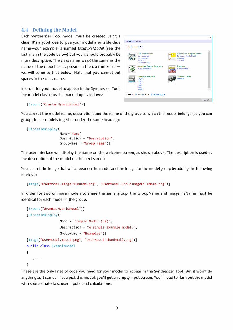
4.4 Defining the Model Each Synthesizer Tool model must be created using a
class. It’s a good idea to give your model a suitable class
name—our example is named ExampleModel (see the
last line in the code below) but yours should probably be
more descriptive. The class name is not the same as the
name of the model as it appears in the user interface—
we will come to that below. Note that you cannot put
spaces in the class name.
In order for your model to appear in the Synthesizer Tool,
the model class must be marked up as follows:
[Export("Granta.HybridModel")]
You can set the model name, description, and the name of the group to which the model belongs (so you can
group similar models together under the same heading):
[BindableDisplay(
Name="Name",
Description = "Description",
GroupName = "Group name")]
The user interface will display the name on the welcome screen, as shown above. The description is used as
the description of the model on the next screen.
You can set the image that will appear on the model and the image for the model group by adding the following
mark up:
[Image("UserModel.ImageFileName.png", "UserModel.GroupImageFileName.png")]
In order for two or more models to share the same group, the GroupName and ImageFileName must be
identical for each model in the group.
[Export("Granta.HybridModel")]
[BindableDisplay(
Name = "Simple Model (C#)",
Description = "A simple example model.",
GroupName = "Examples")]
[Image("UserModel.model.png", "UserModel.thumbnail.png")]
public class ExampleModel
{
. . .
}
These are the only lines of code you need for your model to appear in the Synthesizer Tool! But it won’t do
anything as it stands. If you pick this model, you’ll get an empty input screen. You’ll need to flesh out the model
with source materials, user inputs, and calculations.

10
4.5 Adding Source Materials to the Model Source Materials are created by adding fields to the model class and marking them as materials.
The type of each source material field must be the name of the class in which you defined and stored the
source material properties (as in section 4.3)—in our example, that class is named SourceData.
For example, we can define a field for the matrix material in our model:
public SourceData matrix;
Mark up each source material field as follows:
[Material]
[Display(Name = "Name", Description = "Description")]
The "Name" value is used to label the material in the ‘Source Records’ section of the user interface and the
"Description" is used to provide extra information in the form of a tooltip. The "Name" label also appears in
the ‘Record Naming’ section at the bottom of the user interface; this is where the user enters abbreviations
for the source materials so that suitable record names can be created for the resulting records. The Synthesizer
Tool will generate these user interface elements for you; all you need to provide is the name and description.
You can add as many materials as you like. The example below shows the two materials required for our hybrid
material—a matrix and a reinforcement:
public class ExampleModel
{
[Material]"Matrix", "Matrix material")]
[Display(Name = "Matrix", Description = "Matrix material")]
public SourceData matrix;
[Material]
[Display(Name = "Reinforcement", Description = "Reinforcement material")]
public SourceData reinforcement;
}
4.6 Adding Model Variables The Synthesizer Tool is capable of calculating a family of records in one analysis. This can be achieved by
defining a user specified model variable, such as the reinforcement volume fraction in the Simple model
example.
Model variables can be specified either as a range of discrete values – with start and end values, and a number
specifying the steps in between—or as a list of given values. Note, model parameters, which are single value
constants that can be specified by the user, are discussed in the advanced model example (see section 6.1).
You will typically use one or more variables in your calculation code, and for each one, the Synthesizer Tool
will fill in your field with each specified value in turn. This means that your calculation methods will be called
several times—once for each value or combination of values.

11
Variables are added to the model by creating a field of type double in the model class and marking it as a
variable by using the following, where the Name and Unit are shown in the user interface, and the Description
is used as a tooltip:
[Variable("Unit")]
[Display(Name = "Name", Description = "Description")]
Optionally, you can specify default values for the variable, either as a list or as a range: [Values(10, 20, 30)] [RangeValues(Start = 1, End = 25, Number = 5)]
In the example below, we have created a variable which we’ve named percentage. It holds values for
reinforcement volume fraction (%), defaulting to seven numbers between 10 and 70. By default, values within
a range are created at logarithmic intervals, but in this Simple example we just want linear values, and so we’ve
added logarithmic=false. We have also defined bounds that specify that the values cannot go below 0 or
above 70. The bounds are used by the Synthesizer Tool to validate the user input and make sure that the user
enters valid values for the model variables.
[Variable("%")]
[Display(Name = "Reinforcement percentage", Description = "Specify the volume fraction")]
[RangeValues(Start = 10, End = 70,
Number = 7, Logarithmic = false)]
[Bounds(0, 70)]
public double percentage;
4.7 Calculations By now you should have enough input data available to
perform the real work of the model—the calculations.
Remember that calculations form the behavior of the
model, and are written as methods in the model class.
You’ll need to write a calculation method for each
material property that you want to calculate.
The method must return the calculated value as a value
of type double, and be marked up as calculation data:
[CalculatedData("Property Name", "unit")]
Just like the markup added to source materials, you
should specify the name of the material property you are calculating, plus the unit that you are returning the
result in. Note, the “Property Name” needs to be identical to a property in the installed database if you want
the calculated data to be available for selection projects. If the “Property Name” does not match any of the
properties in the database, the calculated property will be added to the Notes field at the bottom of the
synthesized record’s datasheet.
Calculation methods are called automatically by the Synthesizer Tool, which will set the values of the
parameters and variables accordingly. You can add as many calculation methods as your model needs and
they will all be called by the Synthesizer Tool once for each combination of variables. As our example stands,
this means that the calculation code is called seven times (we have seven reinforcement values) and the model
will create seven synthesized records, each with a different value for reinforcement.

12
Recall that our simple model is calculating density and Young’s modulus for a hybrid material using the rule of
mixtures:
Density, �̃� = 𝑓𝜌𝑟 + (1 − 𝑓)𝜌𝑚
Young’s Modulus, �̃� = 𝑓𝐸𝑟 + (1 − 𝑓)𝐸𝑚
The example code below shows two methods that calculate density and Young’s modulus. Note that:
The method name is followed by an empty pair of brackets ( ).
The calculation code is enclosed in a pair of curly brackets { }.
The word return tells the method to return the result of the calculation.
The model has already been set up to ask for reinforcement volume fraction (𝑓) as a percentage. This is
assigned to the variable percentage. In the calculations below, this is divided by 100 to convert it into a
fraction.
When adding calculations to your model it is important to remember that the source data will be provided in
the requested ‘Data’ unit (see section 4.3) and that the calculated value will be returned in the specified
‘Calculated Data’ unit. As a result, it is important to ensure that your equations are set up to calculate in these
units:
[CalculatedData("Density", "kg/m^3")]
public double Density()
{
return (percentage / 100.0) * reinforcement.Density
+ (1 - percentage / 100) * matrix.Density;
}
[CalculatedData("Young's modulus", "GPa")]
public double YoungsModulus()
{
return (percentage / 100.0) * reinforcement.YoungsModulus
+ (1 - percentage / 100) * matrix.YoungsModulus;
}
Note: calculation methods calculate a point value for each property. If the material data in the installed
database is saved as a range value (e.g., Young’s modulus = 2.0 – 2.9 GPa), these will be converted to point
values using the geometric mean (i.e., square root of the product of the min and max values).

13
5 Running the Model
5.1 Building the Model Once you have created your model, the next step is to compile the model. To do this:
1. Go to the Build menu in Visual Studio and select Configuration Manager. In the resulting dialog,
ensure that the current project is configured to build in ‘Release’ mode by adjusting the drop-down
list in the Configuration column. Once this is done, close the dialog.
2. Go to the Build menu in Visual Studio and select Build Solution. If you’ve made an error you’ll be told.
The module won’t compile and you’ll need to fix the problem (typically this will be an error in syntax,
such as a missing ‘}’ or ‘;’). Assuming that the solution compiled successfully, you can add the model
to the software.
5.2 Adding the Model to the Software The CES EduPack or CES Selector software won’t be able to use your new Synthesizer Tool model until you put
the compiled module in the correct place. The module builds to a .dll file under the bin\Release folder of the
sample, but we need to move it to a place where CES can find it.
To do this, you should make a folder under your CES EduPack or CES Selector installation named plugins. The
software is normally installed under C:\Program Files (x86)\, but if you are running a 32 bit operating system,
you’ll find it under C:\Program Files\. Copy the model .dll file to the plugins folder, as shown below. The .dll
file you need is the one that matches your Visual Studio project name. The other files in the release folder are
not necessary—this is the only file that you need to copy. Note that you might require administrator privileges
to do this.
Now start CES EduPack or CES Selector. When you run the Synthesizer Tool, you should see your new model
in the list of available models.

14
6 Defining a Model: Part 2—Extra Features In this section we will introduce several new concepts that will simplify the definition of calculations.
6.1 Adding Model Parameters Model parameters are similar to model variables, except they can only take a single value rather than varying
across a range or list. To add a parameter, add a field of type double to the model class and mark it as a
parameter as follows:
[Parameter("Unit")]
[Display(Name = "Name", Description = "Description")]
Just like variables, parameters can be constrained to certain values by using [Bounds(LowerBound,
UpperBound)].
As an example, if we want the user to supply a single value for “Parameter X”, we can define it as a model
parameter:
[Parameter("%")] [Display(Name = "Parameter", Description = " Specify a value for X ")] [Bounds(LowerBound = 0)] public double percentage = 10;
Note, in the example above, a default value of 10 has been specified as part of the field definition.
6.2 Using Calculated Parameters Sometimes there is benefit in simplifying calculations by pre-calculating certain values. For example, in the
Simple model we can simplify the density and Young’s modulus calculations by pre-calculating the volume
fraction of reinforcement (fr) and matrix (fm). As we don’t want these values to be added to the resulting
datasheet, these calculations will be marked as private. If percentage is the reinforcement percentage, then
the fractional values are defined as:
fr = percentage / 100
fm = 1 – ( percentage / 100 )
Written as code, this becomes:
private double fr { get { return (percentage / 100); } } private double fm { get { return (1 - percentage / 100); } }
The values for fr and fm can then be used in the existing density and Young’s modulus equations as follows:
[CalculatedData("Density", "kg/m^3")]
public double Density()
{
return fr * reinforcement.Density + fm * matrix.Density;
}

15
[CalculatedData("Young's modulus", "GPa")]
public double YoungsModulus()
{
return fr * reinforcement.YoungsModulus + fm * matrix.YoungsModulus;
}
We could also use this technique if we want to add price (�̃�). If we assume that the price of a hybrid material
is based simply on the cost of the constituent components, then the price can be defined as follows:
Price, �̃� =𝑓𝑟.𝜌𝑟.𝐶𝑟+𝑓𝑚.𝜌𝑚.𝐶𝑚
�̃�
In this case, the method to calculate price will use three pre-calculated values, the public double �̃� (the density
of the final hybrid material), which we have already defined as one of the model calculations (see section 4.7)
and the fr and fm values:
[CalculatedData("Price", "currency/kg")] public double Price()
{
return (fr * reinforcement.Density * reinforcement.Price + fm * matrix.Density *
matrix.Price) / Density();
}
In order for this method to access the price of the reinforcement and matrix materials, the following field must
be added to the SourceData class:
[Data("Price", "currency/kg")] public double Price;
6.3 Using Equation Logic and Standard Functions In certain cases, the performance of a material will be dependent on how the material behaves under certain
load conditions. For example, the compressive strength of unidirectional composites is determined by the
stress at which compressive fiber failure and fiber kinking occurs, with the final strength being determined by
the failure mechanism that occurs at the lowest load. As a result we can define the compressive strength
calculation as follows,
Lesser of {
𝜎�̃� = 0.75 𝑓𝜎𝑐,𝑟 + (1 − 𝑓)𝜎𝑐,𝑚 : compressive fiber failure
𝜎�̃� = 14 𝜎𝑦,𝑚 : fiber kinking
We’ll need to write a little bit of logic to return the correct result. The method shown in the example below
calculates both possible values for compressive strength and then uses the built-in Math.Min method to return
the minimum of these two values:
[CalculatedData("Compressive strength", "MPa")] public double CompressiveStrength() { var cs1 = 0.75 * fr * reinforcement.CompressiveStrength +
fm * matrix.CompressiveStrength; var cs2 = 14.0 * matrix.YieldStrength; return Math.Min(cs1, cs2);
}

16
In order for this method to access the compressive strength and yield strength of the reinforcement and matrix materials, the following fields must be added to the SourceData class:
[Data("Compressive strength", "MPa")] public double CompressiveStrength; [Data("Yield strength (elastic limit)", "MPa")] public double YieldStrength;
Note: there are a number of built-in fields and functions that are frequently used in scientific equations, e.g., Pi, Pow, Sqrt, Min, Max, Log, Log10, Exp, Sin, Cos, Tan. More information on these, and numerous other functions, can be found at:
http://msdn.microsoft.com/en-us/library/system.math.aspx
7 Defining a Model: Part 3—Advanced Features The code associated with the features explained in this section is listed in full in Appendix A and is incorporated
in the Advanced model sample file.
7.1 Reusing Calculations In our model we calculate density, Young’s modulus, and price using the rule of mixtures (RoM):
Density, �̃� = 𝑓𝜌𝑟 + (1 − 𝑓)𝜌𝑚
Young’s Modulus, �̃� = 𝑓𝐸𝑟 + (1 − 𝑓)𝐸𝑚
Price, �̃� =𝑓𝜌𝑟.𝐶𝑟+(1−𝑓)𝜌𝑚.𝐶𝑚
�̃�
When we implemented this in the Simple model, we wrote the RoM calculation out in full for each property.
However, we can improve that code by creating a calculation method for the rule of mixtures and calling it
from the Density, Young’s Modulus, and Price methods. To do so, we create a method that takes two values
for the source material and returns the value for the hybrid material using the reinforcement percentage,
percentage. The code for the other calculations can then use this method, as shown below:
[CalculatedData("Density", "kg/m^3")] public double Density() { return RuleOfMixture(reinforcement.Density, matrix.Density); } [CalculatedData("Young's modulus", "GPa")] public double YoungsModulus() { return RuleOfMixture(reinforcement.YoungsModulus, matrix.YoungsModulus); } [CalculatedData("Price", "currency/kg")] public double Price() { return RuleOfMixture(reinforcement.Density * reinforcement.Price,
matrix.Density * matrix.Price) / Density() ; } private double RuleOfMixture(double a, double b) { var f = percentage / 100;

17
return f * a + (1.0 - f) * b; }
Note that the RuleOfMixture method has been defined as private: it is not visible outside the model class.
7.2 Adding a List of Options In certain models you may want the user to pick a parameter value from a list of options. This is shown in the
Synthesizer Tool user interface as a drop-down list. To do this, we need to use something known as an
enumeration, or enum. An enumeration defines a list or a set of named values that a field can take. We are
going to extend our example model to allow the user to specify whether the reinforcement orientation is
unidirectional or quasi-isotropic. To do so, we will create an enumeration that lists these two options, and a
field to hold the option that the user has selected.
The example below creates an enum named
LaminateType that can take two values—Unidirectional
and QuasiIsotropic. The [OptionItem] markup is added to
specify what is displayed in the Synthesizer Tool user
interface, specifically the two entries in the ‘Laminate’
drop-down list.
To make use of whichever option the user selects, we
create a field of the enum type (LaminateType) and mark
it as an option. The Name is used to label the option in
the user interface, and the Description is used as a
tooltip:
[Option] [Display(Name = "Name", Description = "Description")]
Here is the code for creating a list of options, and setting the default value to Unidirectional:
public enum LaminateType { [Display(Description = "Unidirectional fiber")] Unidirectional, [Display(Description = "Quasi-isotropic fiber")] QuasiIsotropic, } [Option] [Display(Name = "Laminate", Description = "Pick a laminate")] public LaminateType laminate = LaminateType.Unidirectional;
The code below uses the value of the laminate field to modify the calculation of Young’s modulus. If the
laminate is Unidirectional, the calculation simply uses the rule of mixtures, but if the laminate is Quasi-
Isotropic, the rule of mixtures is calculated using only 0.5 of the reinforcement value. We are using a switch
statement to change the calculation based on the laminate type. In practice the value of the field laminate will
always be set to Unidirectional or Quasi-Isotropic and a suitable value calculated, but we need to cater for the
hypothetical case where the fields is blank, otherwise we will get a compilation error. This is handled by the
default statement, which returns a special constant, double.NaN, which simply means that the model failed
to calculate a value.

18
[CalculatedData("Young's modulus", "GPa")] public double YoungsModulus() { switch (laminateType) { case LaminateType.Unidirectional: return RuleOfMixture(reinforcement.YoungsModulus, matrix.YoungsModulus); case LaminateType.QuasiIsotropic: return RuleOfMixture(0.5 * reinforcement.YoungsModulus, matrix.YoungsModulus); default: return double.NaN; } }
7.3 Modifying Record Naming To assist with creating meaningful and unique names for synthesized records, a model can be configured to
take abbreviated names for the source materials, in the ‘Record Naming’ section of the user interface. The
Synthesizer Tool will automatically generate an appropriate name for the resulting records based on these
abbreviated names. To add these abbreviated names, use the following markup for each source material:
[RecordName] [Display(Name = "Name", Description = "Description")]
For instance, for the example model, the names “Matrix” and “Reinforcement” could be used to generate a
meaningful name for each record produced by the model:
[RecordName] [Display(Name = "Matrix", Description = "Abbreviation used in record name")]
[RecordName] [Display(Name = "Reinforcement", Description = "Abbreviation used in record name")]
7.4 Arranging the Layout of the User Interface As you have seen, the Synthesizer Tool will automatically create a user interface based on the custom model.
However, it is possible to set the order in which the elements appear on the user interface. This can be
achieved using the following markup:
[Group(“GroupName”, orderNumber)]
Elements marked with the same GroupName will appear
together in the user interface. The order number (which
should not be enclosed in quotation marks) is used to
specify the order in which the element appears in the
user interface. The numbering does not need to be
sequential. For best results, it is recommended that
numbering is unique across the groups in the order in
which you wish the elements to appear. The advanced
example model uses this feature to override the default
element arrangement:
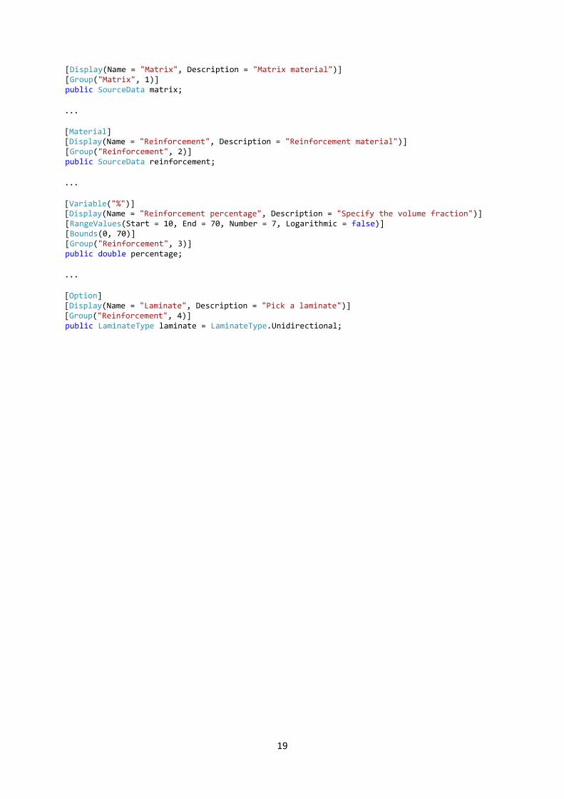
[Material]
19
[Display(Name = "Matrix", Description = "Matrix material")] [Group("Matrix", 1)] public SourceData matrix;
...
[Material] [Display(Name = "Reinforcement", Description = "Reinforcement material")]
[Group("Reinforcement", 2)] public SourceData reinforcement;
...
[Variable("%")] [Display(Name = "Reinforcement percentage", Description = "Specify the volume fraction")]
[RangeValues(Start = 10, End = 70, Number = 7, Logarithmic = false)] [Bounds(0, 70)] [Group("Reinforcement", 3)] public double percentage;
...
[Option] [Display(Name = "Laminate", Description = "Pick a laminate")] [Group("Reinforcement", 4)]
public LaminateType laminate = LaminateType.Unidirectional;

20
7.5 Changing Model Images Models can be grouped so that, when the Synthesizer Tool is opened, the models appear in the same section
of the user interface. Each group has a thumbnail image and, when clicked, each model has its own image.
As explained in section 4.4 (Defining the model) above, the image for each model and the thumbnail image for
a group of models is set by marking up the model class with the following:
[Image("UserModel.model.png", "UserModel.thumbnail.png")]
thumbnail.png is the image used for the thumbnail image and is 64 pixels wide and 64 pixels high. model.png
is the image displayed at the top of each model and is 200 pixels wide and 125 pixels high.
These images can be replaced with your own custom images provided that:
1. the image is in .png format;
2. the image is of the correct dimensions;
3. the name of the image matches the name as set out in the model code; and
4. the image is located in the same file directory as the Visual Studio project.
21
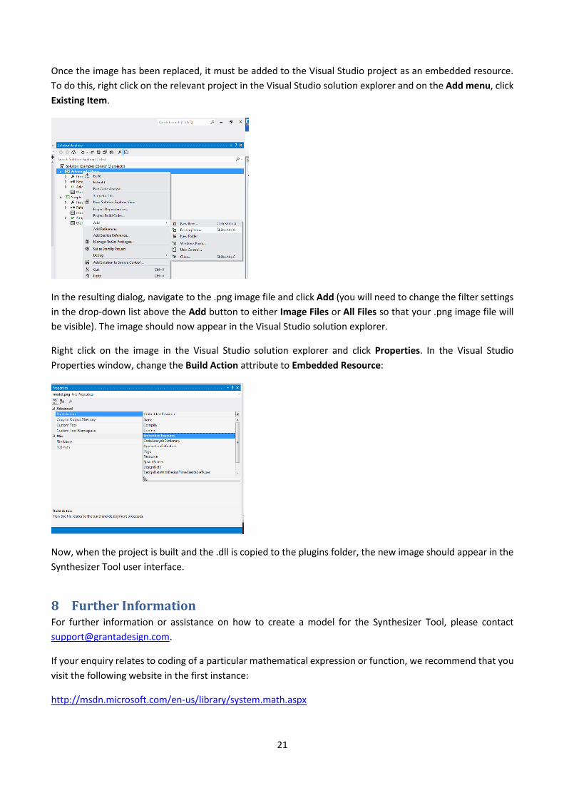
Once the image has been replaced, it must be added to the Visual Studio project as an embedded resource.
To do this, right click on the relevant project in the Visual Studio solution explorer and on the Add menu, click
Existing Item.
In the resulting dialog, navigate to the .png image file and click Add (you will need to change the filter settings
in the drop-down list above the Add button to either Image Files or All Files so that your .png image file will
be visible). The image should now appear in the Visual Studio solution explorer.
Right click on the image in the Visual Studio solution explorer and click Properties. In the Visual Studio
Properties window, change the Build Action attribute to Embedded Resource:
Now, when the project is built and the .dll is copied to the plugins folder, the new image should appear in the
Synthesizer Tool user interface.
8 Further Information For further information or assistance on how to create a model for the Synthesizer Tool, please contact
If your enquiry relates to coding of a particular mathematical expression or function, we recommend that you
visit the following website in the first instance:
http://msdn.microsoft.com/en-us/library/system.math.aspx

22
Appendix A—Source Listing (Advanced Model) using System; using System.ComponentModel.Composition; using Granta.HybridBase; using Granta.Framework.DataAnnotations; using System.ComponentModel.DataAnnotations; namespace UserModel { #region Source Material Data Definition public class SourceData { [Data("Density", "kg/m^3")] public double Density; [Data("Young's Modulus", "GPa")] public double YoungsModulus; [Data("Compressive strength", "MPa")] public double CompressiveStrength; [Data("Yield strength (elastic limit)", "MPa")] public double YieldStrength; // When requesting price data, the unit takes the form currency/kg: [Data("Price", "currency/kg")] public double Price; } #endregion [Export("Granta.HybridModel")] [BindableDisplay(Name = "Advanced Model (C#)",
Description = "A more advanced example model.", GroupName = "Examples")]
[Image("UserModel.model.png")] public class ExampleModel { [Material] [Display(Name = "Matrix", Description = "Matrix material")] [Group("Matrix", 1)] public SourceData matrix; [RecordName] [Display(Name = "Matrix", Description = "Abbreviation used in record name")] public string _matrixName; [Material] [Display(Name = "Reinforcement", Description = " Reinforcement material")] [Group("Reinforcement", 2)] public SourceData reinforcement; [RecordName] [Display(Name = "Matrix", Description = "Abbreviation used in record name")] public string _reinforcementName; [Variable("%")] [Display(Name = "Reinforcement percentage", Description = "Specify the volume fraction")] [RangeValues(Start = 10, End = 70, Number = 7, Logarithmic = false)] [Bounds(0, 70)] [Group("Reinforcement", 3)] public double percentage;
23
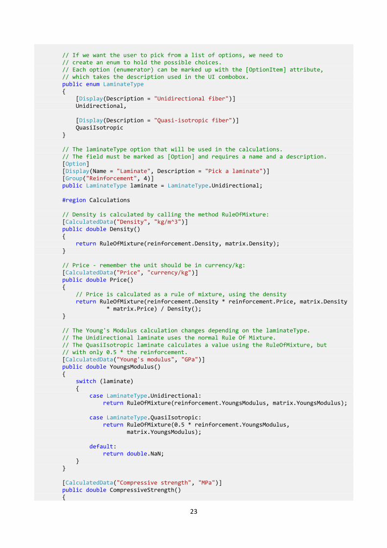
// If we want the user to pick from a list of options, we need to // create an enum to hold the possible choices. // Each option (enumerator) can be marked up with the [OptionItem] attribute, // which takes the description used in the UI combobox. public enum LaminateType { [Display(Description = "Unidirectional fiber")] Unidirectional, [Display(Description = "Quasi-isotropic fiber")] QuasiIsotropic } // The laminateType option that will be used in the calculations. // The field must be marked as [Option] and requires a name and a description. [Option] [Display(Name = "Laminate", Description = "Pick a laminate")] [Group("Reinforcement", 4)] public LaminateType laminate = LaminateType.Unidirectional; #region Calculations // Density is calculated by calling the method RuleOfMixture: [CalculatedData("Density", "kg/m^3")] public double Density() { return RuleOfMixture(reinforcement.Density, matrix.Density); } // Price - remember the unit should be in currency/kg: [CalculatedData("Price", "currency/kg")] public double Price() { // Price is calculated as a rule of mixture, using the density return RuleOfMixture(reinforcement.Density * reinforcement.Price, matrix.Density * matrix.Price) / Density(); } // The Young's Modulus calculation changes depending on the laminateType. // The Unidirectional laminate uses the normal Rule Of Mixture. // The QuasiIsotropic laminate calculates a value using the RuleOfMixture, but // with only 0.5 * the reinforcement. [CalculatedData("Young's modulus", "GPa")] public double YoungsModulus() { switch (laminate) { case LaminateType.Unidirectional: return RuleOfMixture(reinforcement.YoungsModulus, matrix.YoungsModulus); case LaminateType.QuasiIsotropic: return RuleOfMixture(0.5 * reinforcement.YoungsModulus, matrix.YoungsModulus); default: return double.NaN; } } [CalculatedData("Compressive strength", "MPa")] public double CompressiveStrength() {

24
switch (laminate) { case LaminateType.Unidirectional: { var cs1 = RuleOfMixture(0.75 * reinforcement.CompressiveStrength, matrix.CompressiveStrength); var cs2 = 14.0 * matrix.YieldStrength; return Math.Min(cs1, cs2); } case LaminateType.QuasiIsotropic: { var cs1 = RuleOfMixture(0.25 * reinforcement.CompressiveStrength, matrix.CompressiveStrength); var cs2 = 14.0 * matrix.YieldStrength; return Math.Min(cs1, cs2); } default: return double.NaN; } } #endregion // The Rule Of Mixture implemented as a helper method, and reused in the calculations above. private double RuleOfMixture(double a, double b) { var f = percentage / 100; return f * a + (1.0 - f) * b; } } }

25
Appendix B—Model References and Properties In order to build a model, you’ll need to add a reference to the Synthesizer library. You can do this by right-
clicking on the project name e.g., ‘Simple.CSharp’, and selecting Add Reference from the context menu, as
shown in the screen below:
In the Reference Manager, click Browse. Browse to the installation folder for CES EduPack or CES Selector
(e.g., C:\Program Files (x86)\CES xxxxxxx\) and select (by holding down the Ctrl key) Granta.Data.dll,
Granta.Framework.dll and Granta.HybridBase.dll. Click Add to add the reference.

26
Similarly, add a reference to the Microsoft.Net libraries System.ComponentModel.Composition and
System.ComponentModel.DataAnnotations as shown in the screen below. In the Reference Manager, click
Assemblies, then click Framework. To find the library, use the scroll bar or the search in the top right of the
Reference Manager. If there are several versions of the library available, check the box for the 4.0 version.
Click OK to close the Reference Manager.
You can also change the output file name (.dll) by using the Project menu and selecting
<your project name> Properties (the last entry in the menu). The window should appear as shown below,
where, under Application, you can modify the Assembly name to reflect that of your model. Now when you
build your model, it will create a .dll with your model name.

27
Appendix C—Debugging the Model
Set the project configuration to Debug. Now your model should build to the bin\debug folder rather than the
bin\release folder. Remember that each time you make a change to your model; you must rebuild the solution
and copy the output .dll to the CES EduPack or CES Selector plugins folder.
If you try to debug your model (using Debug -> Start debugging) you’ll be greeted with an error message
saying that a project with an output type of Class Library cannot be started directly. You can’t run the model
directly as it is a library, not an application, and runs inside CES. Instead, you can debug your library by
attaching to a running CES.exe.
You can do this as follows:
1. Start CES EduPack or CES Selector as normal.
2. On the Debug menu in Visual Studio, click Attach to Process....
3. In the resulting dialog, find CES.exe in the list of Available Processes and select it. Click Attach.