1

Student Name: Krishan Rayarel

Module: L13500 Economics Dissertation 2018

Supervisor: Spiros Bougheas

Word Count: 7,345

This Dissertation is presented in part fulfilment of the requirement for the completion of an

Undergraduate degree in the School of Economics, University of Nottingham. The work is the

sole responsibility of the candidate.

I am happy for this dissertation to be made available to students in future years if chosen as an

example of good practice.

Abstract:

This study tests the efficient market hypothesis (EMH) by analysing the effect of Donald Trump’s

company-specific tweets on financial markets for the period between 8 November, 2016 (the U.S.

presidential election date) to 24 January, 2018 (a year after inauguration). Using a sample of 24

company-specific tweets, the results show that a tweet by Trump leads to statistically significant

abnormal returns that last for 2 to 3 trading days. This is inconsistent with the semi-strong form

of EMH. This is the first paper to test the attention-based investing hypothesis by Barber and

Odean (2005) using Trump’s tweets. Attention-based investing is a possible reason for market

inefficiency as Trump’s tweets lead to an abnormal trade volume of 43.54% on the day of the

tweet and an increase in Google search activity on the week of the tweet.

The Impact of Donald Trump’s Tweets on

Financial Markets

2

1. Introduction ..................................................................................................................... 3

2. Background ...................................................................................................................... 4

3. Literature Review ............................................................................................................. 5

4. Data .................................................................................................................................. 8

4.1. Tweet Collection

4.2. Financial Data Collection

4.3. Sentiment Classification

5. Methodology .................................................................................................................... 9

5.1. Event Studies

5.1.1. Sample Selection

5.1.2. Normal and Abnormal Returns

5.1.3. Significance Tests for AAR & CAAR

5.2. Average Abnormal Trading Volume (AAV)

5.2.1. Significance Tests for Average Abnormal Trading Volume

5.3. Google Search Activity

5.4. Hypotheses

6. Results: Testing the Efficient Market Hypothesis (EMH) ........................................... 17

6.1. Market Model Coefficients

6.2. Average Abnormal Returns (AAR)

6.3. Cumulative Average Abnormal Returns (CAAR)

7. Results: Testing for Attention-Based Investing ............................................................. 22

7.1. Average Abnormal Trading Volume (AAV)

7.2. Google Search Activity

8. Discussion ....................................................................................................................... 23

8.1. General Analysis

8.2. Justifications

8.3. Limitations

9. Conclusion ...................................................................................................................... 24

10. Bibliography .................................................................................................................. 26

11. Appendices .................................................................................................................... 28

3

1. Introduction

The social networking platform Twitter was established in 2006. It has since grown in popularity

with over 330 million active users (Statista, 2018). An avid user of Twitter is Donald Trump.

Recently elected as the 45th President of the United States, Trump, unlike his 44 predecessors,

actively uses Twitter to express his views on global affairs. One would think that Trump uses

Twitter to build support for his campaign however, Trump is renowned for using Twitter as a

strategic tool to prevent US companies from moving operations overseas and publicly berating

political leaders. With over 50 million followers on Twitter, Trump has become the most

followed world leader and investors are now closely monitoring his tweets as indicators of future

policy. This gives Trump exclusive power to influence financial markets with just 140 characters,

as shown below:

Trump tweeted about Lockheed Martin on 22 December, 2016 after the market had closed. The

next trading day, Lockheed Martin’s stock price dropped by 2% and this decreased its market

value by $1.2 billion. Trump may have been able to move the market this much because

investors feel Lockheed Martin will be targeted by Trump in future policy and therefore this new

information is reflected today through a decrease in its stock price. Figure 1 also shows that the

stock recovered on the same day. This may imply markets rapidly incorporate new information

and thus the efficient market hypothesis (EMH) holds.

Figure 1: 1-minute chart of Lockheed Martin’s (LMT) stock price.

4

On the other hand, some of Trump’s tweets are non-informative. For instance, Trump

responded to Nordstrom’s announcement of removing Ivanka Trump’s clothing line:

@realDonaldTrump: “My daughter Ivanka has been treated so unfairly by @Nordstrom. She is a

great person – always pushing me to do the right thing! Terrible!”

This tweet merely draws attention to Nordstrom’s actions and is non-informative. Immediately

after the tweet, Nordstrom’s stock plummeted by -0.3%. However, after just 4 minutes

(Marketwatch, 2017) the stock price recovered and at market close, the stock price had actually

increased by 4%. The fact that the market reacts to a non-informative Trump tweet, suggests

that the EMH does not hold. A possible explanation of these movements is Trump’s tweets

catch the attention of retail investors1 who cannot process all available information. This paper

tests this hypothesis.

These examples highlight that analysing the impact of Trump’s tweets on financial markets is a

unique way of testing the EMH. Specifically, this paper will first test the hypothesis that a

positive (negative) Trump tweet leads to a higher (lower) stock return. The study will then test

whether stock prices rapidly incorporate the informational content of Trump’s tweets, thus

testing the semi-strong form of the EMH. Finally, this paper tests the attention-based investing

hypothesis by Barber and Odean (2005) through analysis of trading volume and Google search

activity.

2. Background

Eugene Fama (1965) pioneered the EMH, which states that all available information at a certain

time is fully incorporated into security prices. The intuition behind this is that, in the absence of

frictions, this information disperses so quickly that security prices adjust before an investor has

time to trade. There are three forms of the EMH; the semi-strong form is analysed in this paper.

This form states that all public announcements are priced into the market. Public

announcements may include earnings announcements and dividend changes. By classing

Trump’s tweets as public announcements, the semi-strong form of EMH is tested.

The literature review shows that there is no consensus on whether the EMH holds in practice.

One possible reason for this is that the EMH assumes that investors consider all available

1 A retail investor is a non-professional investor that trades for personal reasons rather than for an institution. They tend to trade in much smaller amounts than institutional investors do. They have fewer resources to work with.

5

information when investing. When choosing what to invest in, investors have the option of

many different stocks. Barber and Odean (2005) suggest retail investors have high search costs

and therefore are likely to only consider information that grabs their attention rather than all

available information. On the other hand, institutional investors are less prone to indulge in

attention-based purchases as they have relatively more time and resources. This means that the

EMH does not hold, as some investors do not consider all available information. This study will

test this hypothesis by analysing abnormal trading volume to assess whether a tweet by Trump

does actually generate investor attention. Furthermore, this study will contribute to Barber and

Odean (2005) as it will monitor the Google search activity of these stocks during Trump’s

tweets. Google search activity determines whether small retail investors act upon Trump’s tweets

and drive market inefficiency, assuming small retail investors are likely to use Google to search

for stocks, unlike institutional investors who will use Bloomberg Terminals.

3. Literature Review

The EMH appears frequently in economic literature. A common methodology used to test the

EMH is event studies2. This dissertation also uses event studies and therefore, the review starts

by comparing key event study papers. These papers tend to analyse the effect of financial

announcements, such as stock splits, on markets. Recently, Economists have focused on the

impact of non-financial announcements, such as social media posts, on stock markets to test the

EMH. Trump’s tweets are non-financial announcements and therefore key papers that analyse

the effect of these specific announcements on financial markets will be the focus of the latter

parts of the review.

Fama, Fisher, Jensen and Roll (1969) were the first to test the semi-strong form of EMH using

event studies. They analysed the impact of stock splits3 on stock prices using monthly data. They

pioneered the market model4 in order to control for general market movements and focus purely

on the effect of the stock split announcement. In the pre-announcement period, the returns on

stocks are very high. This is because these companies have experienced dramatic increases in

expected earnings and dividends, leading to an increase in stock price (hence the need for the

stock split). The returns on these securities are even higher a few months after the split. This

implies that the market is inefficient as it takes time to incorporate this new information.

However, the authors note that co-existing events could be driving stock price changes. More

2 Event studies are a statistical method used to measure the impact of an event on a firm’s value or stock price 3 A stock split is a way of reducing the stock price of the company in order to make the stock more affordable to investors. 4 A market model is a statistical method of finding expected returns of stocks. It is devised through a regression, which will be shown in the methodology section.

6

specifically, dividend payments usually change after a stock split and therefore this may affect the

stock price. Once they control for dividend announcements, abnormal returns5 are insignificant

for periods after the stock split announcement. This means that the market is efficient as stock

prices adjust rapidly to new information. Similarly, this dissertation uses event studies and the

market model to test stock market efficiency. In contrast, instead of using monthly data, this

study uses daily data as Trump is likely to have a short-term effect on stock prices. This paper by

Fama et al. (1969) initiated an array of research on the effect of different types of public

announcements on financial markets such as dividend policy changes and quarterly earnings

announcements.

Charest (1978) analysed the impact of dividend changes on the stock prices of New York Stock

Exchange (NYSE) companies over the period 1947-1967. He finds that an increase in cash

dividend leads to abnormal returns of 1%. A decrease in cash dividend leads to abnormal returns

of -3.18%. He suggests there is a stronger negative effect as a decrease in cash dividend

announcement is usually in the wake of other bad news. Moreover, he finds significant abnormal

returns in the months following dividend changes. This implies the market is inconsistent with

the semi-strong form of EMH. Similarly, Ball and Brown (1968) found evidence inconsistent

with the semi-strong form of EMH. However, they analysed the impact of annual corporate

earnings announcements on security prices. They found that stock prices do not fully

incorporate new information instantly and abnormal returns are present many days after the

announcement. They call this the post earnings announcement drift (PEAD) and it represents

the delay in stock price adjustment to equilibrium levels. Bernard and Thomas (1989) test the

EMH through analysis of quarterly earnings announcements on stock prices. Similarly, to Ball

and Brown (1968), they find a PEAD of 60 days. Therefore, these findings are inconsistent with

the EMH. Many studies analyse the impact of financial announcements on stock markets. This

dissertation contributes to the existing literature by focusing on a non-financial announcement.

Specifically, it focuses on how social media posts can affect financial markets.

The growing influence of media and social media has led to a flurry of research into the impact

of media on financial markets. Tetlock (2007) analyses the interactions between a popular Wall

Street Journal column and the stock market. In this journal column, brokerage houses, Analysts

and other professionals give their views on stocks. By categorising the content of these columns

into pessimistic, negative and weakly negative, he finds that high values of media pessimism lead

to temporary downward pressure on corresponding stock prices and temporarily high values of

5 Abnormal returns are the actual returns of a stock minus the expected returns of a stock (which is calculated through the market model).

7

trading volume. This downward pressure lasts for two trading days. After making a fair

assumption that these newspaper columns are non-informative about the fundamentals of the

company, he argues that the market is inconsistent with the semi-strong form of EMH. Ranco et

al. (2015) instead analyse the impact of Twitter on markets. During U.S. earnings season, a

positive tweet leads to a cumulative average abnormal return (CAAR)6 of 4.22% on the day of

the tweet whereas a negative tweet leads to a CAAR of -5.64%. These effects last for up to 10

days after the tweet, implying inconsistency with the semi-strong form of the EMH. Similarly,

positive tweets posted during non-earnings periods lead to a CAAR of 3.65% whereas negative

tweets lead to a CAAR of -3%. These effects last for up to 8 days after the tweet. This confirms

that the EMH does not hold. Similarly, this dissertation analyses the impact of social media on

financial markets, however it focuses on one Twitter user, namely Donald Trump. Ranco et al.

(2015) show that including earnings announcement periods lead to an inflated figure for

abnormal returns. Therefore, in this study, Trump’s tweets that occur during earnings season are

excluded in order to find the exact impact of a Trump tweet.

Malaver and Vojvodic (2017) focus on the effect of Trump’s tweets on the Mexico Peso against

the U.S. Dollar. They analyse the impact of 7,429 Trump tweets between June 16, 2015 and

February 21, 2017. The results show that a negative tweet by Trump leads to an increase in the

daily volatility of the Mexican Peso against the U.S. Dollar by 21.6%. This shows that Trump can

influence foreign exchange markets. This dissertation will focus on stock markets rather than the

foreign exchange market as methods for testing the EMH in foreign exchange markets are not as

widely documented as methods for testing the EMH in stock markets.

Born, Myers and Clark (2017) test the semi-strong form of EMH by analysing the impact of

Trump’s tweets on stock markets. They analyse stock returns during the president-elect period7.

The results show that CAAR are statistically significant for five trading days after the tweet,

implying inefficient markets. They also compute abnormal trading volume and Google search

activity in order to monitor whether noise trading is present. They find that the pattern of

trading volume and Google search activity implies small noise traders are reacting to Donald

Trump’s tweets and therefore driving market inefficiencies. A caveat of this paper is a small

sample size of only 15 tweets. Ge, Kurov and Wolfe (2017) build upon the limitation of Born et

al. (2017) by considering a larger sample size of 48 tweets. They consider tweets from the pre-

6 Cumulative average abnormal returns are simply the sum of average abnormal returns over the event window. This is used to test how long it takes markets to incorporate new information. 7 The president-elect period is a period between the election date and inauguration whereby a candidate has won the election but has not entered office yet. For Trump, this period was between November 8, 2016 and January 20, 2017.

8

inauguration and post-inauguration period8 rather than just the president-elect period. Using

event studies, they find that positive and negative Trump tweets, on average, move stock price

by 0.80% and there is no asymmetry in the impact of positive and negative tweets. They find

abnormal returns are statistically significant for 2 days after the tweet. This is inconsistent with

the semi-strong form of EMH. A limitation of event study methodology is that co-existing

events could move stock prices and therefore have an impact on the sample of stocks. For

instance, preceding company or earnings announcements may cause misinterpretation of the

impact of Trump’s tweets. These papers do not consider the effect of earnings and company

announcements that occur in proximity to Trump’s tweets. Ge et al. (2017) note that only 18 out

of the 48 presidential tweets do not have preceding related news events. To build upon these

limitations, this dissertation categorises Trump’s tweets into informative and non-informative

tweets. Informative tweets are used to test the EMH and non-informative tweets will be

discarded from the sample.

To summarise, this dissertation is building upon the limitations of previous literature. The

sample size of Trump’s tweets is increased by increasing the sample range. 24 tweets are

obtained, which is an enlargement of the sample size of previous literature9. Furthermore, a

subsample of Trump’s tweets that are not responses to company announcements and do not

occur during earnings announcements is created. This subsample is used to test the EMH. The

key contribution of this paper to existing literature is the explanation for why markets may be

inefficient. More specifically, analysis of abnormal trading volume and Google search activity

provides insight on whether Trump’s tweets lead to attention-based investing, which in turn

drives market inefficiency.

4. Data

4.1. Tweet Collection

An algorithm devised by Twlets.com is used to collect a full sample of Trump’s company-

specific tweets. Tweets posted by Donald Trump’s personal account (@realDonaldTrump) are

used rather than Donald Trump’s presidential account (@POTUS) as Trump simply retweets his

personal account tweets on his presidential account and hence activity on this account provides

no new information.

8 Inauguration, in this case, is the ceremony to mark the start of Donald Trump’s presidency. The ceremony was held on January 20, 2017. 9 Considering Ge et al. (2017) have only 18 informative tweets.

9

4.2. Financial Data Collection

Yahoo Finance is used to access historical daily prices of stocks and logarithmic daily stock

returns are calculated using the formula:

Ri,t = ln (Pi,t)

ln (Pi,t−1)

Where (Ri,t) is the daily returns of stock i at time t, Pi,t is the closing price of stock i at day t and

Pi,t-1 is the previous day’s closing price for stock i.

The stocks used are the ones mentioned by Trump in his company-specific tweets. Daily data is

used rather than intraday data as daily data is more accessible and also Trump occasionally tweets

after the market closes so the effect is evident on the next trading day. Furthermore, Trump

tends to tweet about two companies on the same day due to the 140-character limit and daily

returns combines the effect of both tweets on the stock. Similarly, the daily trading volume data

across firms is collected through Yahoo Finance.

4.3. Sentiment Classification

Sentiment analysis is undertaken via an algorithm called valence aware dictionary and sentiment

reasoner (VADER). VADER is a reliable method for calculating the polarity of tweets as it is

used frequently to analyse social media. VADER has a dictionary of social media vocabulary and

matches words in tweets with this dictionary. It assigns a compound value to tweets and

categorises tweets as positive, negative and neutral. Here is an example of VADER analysis on

one Donald Trump tweet:

@realDonaldTrump: “Thank you Brian Krzanich, CEO of @intel. A great investment ($7

BILLION) in American INNOVATION and JOBS!”

The VADER analysis assigns this tweet a compound score of 0.8814. The sentiment score of

each tweet is compounded and standardised between 1 and -1 with 1 being extremely positive, -1

being extremely negative and 0 being neutral. As can be seen, VADER does well in accurately

identifying the sentiment in the above tweet and classing it as a very positive tweet. Trump’s

tweets are classified into positive and negative sentiments in this manner (see appendix C).

10

5. Methodology

5.1. Event Studies

The first step of conducting an event study is to define the event window. The event window is

the time interval over which the event occurs. This can include a certain number of days before

and after the announcement.

Figure 2: Event study timeline

This timeline defines the key periods in an event study. On the timeline, 𝑡 = 0 is the day that the

tweet occurs. This is the event day. The event window is T1-T2 where T1 is the first day in the

event window and T2 is the last day. There is no consensus on the length of the event window.

In existing event study literature, the event window varies from 1 to 40 days. Born et al (2017),

who also measure the effect of Trump’s tweets on financial markets, incorporate a 10-day event

window ranging from day -5 (5 days before the announcement) to day 5 (5 days after the

announcement). A 20-day event window, which analyses average abnormal returns on day -10

and day 10, is incorporated in this study. I use a longer event window than Born et al. (2017) to

confirm there are no preceding events that affect stock returns.

The second step of an event study is to define the estimation window. The estimation window is

the interval of time before the event window that is used to estimate the expected (or normal)

returns. When selecting the estimation window, it is usually common practice, according to

Peterson (1989), to pick an estimation window with a length of 100 to 300 days. The more days

we use, the more accurate the estimation parameters are likely to be. In this study, the estimation

window starts from day -271 and ends on day -21. Therefore, the length of the estimation

window is 250 trading days. There is gap of 10 days between day -21 and day -11, in order to

prevent the tweet from influencing the expected return parameters.

5.1.1. Sample Selection

The second step of conducting an event study is to define the sample. Firstly, Trump tweets a

significant number of times to the New York Times (NYT). Over the sample period, he sent 42

negative tweets to the NYT. It is assumed that markets have factored in Trump’s negative stance

on NYT and therefore these tweets are excluded from the sample. Ge et al. (2017) and Born et

al. (2017) also exclude these tweets. A limitation of event studies is that the results on day 0

11

could be driven by preceding events such as earnings and company announcements. In this

study, company announcements do occur in proximity to a minority of Trump’s tweets. For

instance:

@realDonaldTrump: “Thank you to @exxonmobil for your $20 billion investment that is

creating more than 45,000 manufacturing & construction jobs in the USA!”

The fact that Exxon are investing $20 billion may lead to an increase in their stock price itself

and therefore if this tweet is included in the sample, the effect of Trump’s tweet would be biased

upwards by this company announcement. Therefore, tweets that are responses to company

announcements (henceforth ‘response tweets’) are excluded from the sample as these tweets do

not contain new information. Similarly, a better-than-expected earnings announcement may lead

to an increase in stock price and therefore bias the effect of Trump’s tweets on stock prices.

Therefore, Trump’s tweets which are in a 20-day proximity to earnings announcement dates (see

appendix B) are excluded from the sample when testing the EMH.

Overall, the full data sample contains 44 Trump tweets observed between 8 November, 2016

(the US presidential election date) to 24 January, 2018 (a year after inauguration). 15 tweets are

response tweets, 4 tweets occur during earnings announcements and 1 tweet occurs during a

takeover announcement. These 20 tweets are excluded from the sample. The remaining 24

tweets are informative and this subsample is used to test the EMH. These tweets are categorised

as positive or negative through sentiment analysis and overall we find that out of the 24 tweets,

there are 16 negative tweets and 8 positive tweets.

5.1.2. Normal & Abnormal Returns

Now that the estimation period is defined and the sample is selected, the normal (or expected)

returns of each stock can be calculated. There are three commonly used methods to calculate

normal returns. The constant mean return model (CMR) is a statistical model that postulates

expected returns are simply the mean of returns in the estimation window. Another model is the

market model, which calculates expected return by accounting for general market movements.

This requires an OLS regression of stock return on the market return. Finally, the capital asset

pricing model (CAPM) calculates the expected return by accounting for risk investors bear when

buying a specific stock. The market model is more comprehensive than the CMR as the CMR

does not control for market movements. Brown and Warner (1985) find that the CMR is mis-

specified when there is event clustering. Event clustering occurs when different tweets have

overlapping event windows. This is found as Trump often tweets about two different companies

12

on consecutive days. Therefore, the market model is more suitable than the CMR. In addition,

Brown and Warner (1980) and MacKinlay (1997) find that the market model is a more powerful

test than CAPM for event studies. Therefore, I use the market model to estimate normal returns.

The market model firstly requires an OLS regression:

𝑅𝑖,𝑡 = 𝛼𝑖 + 𝛽𝑖𝑅𝑆&𝑃500,𝑡 + 𝜀𝑖,𝑡

𝐸(𝜀𝑖,𝑡) = 0

Where 𝑅𝑖,𝑡 is the daily return of stock i, 𝛼𝑖 is the intercept, 𝛽𝑖 is the beta of the stock, and

𝑅𝑆&𝑃500,𝑡 is the return of the S&P500 index, which is used as the market proxy. 𝜀𝑖,𝑡 is the error

term which has a mean of zero.

The beta and intercept results and the actual daily return of the S&P500 are then used to find the

daily normal return for each stock. This daily normal return is subtracted from the stock’s actual

return to obtain an estimate of abnormal return for stock i on day t.

𝐸(𝑅𝑖,𝑡) = 𝛼𝑖 + 𝛽𝑖𝑅𝑆&𝑃500,𝑡

𝐴𝑅𝑖,𝑡 = 𝑅𝑖,𝑡 − 𝐸(𝑅𝑖,𝑡)

As Trump tweets about many stocks, the abnormal return of each stock can be combined into a

portfolio and averaged. This is the average abnormal return (AAR):

𝐴𝐴𝑅𝑡 =1

𝑁∑ 𝐴𝑅𝑖,𝑡

𝑁

𝑖=1

Where N is the number of stocks.

To test how quickly the market adjusts to new information, the cumulative average abnormal

returns (CAAR) must be derived. The cumulative average abnormal return is expressed as one

number across different event windows:

𝐶𝐴𝐴𝑅(𝑇1,𝑇2) = ∑ 𝐴𝐴𝑅t

𝑇2

𝑡=𝑇1

Where 𝑇1 is the first day in the event window and 𝑇2 is the last day in the event window.

13

5.1.3. Significance test for AAR & CAAR - Crude Dependence Adjustment (CDA):

Brown and Warner (1980) established the crude dependence adjustment test to check for the

significance of AAR and CAAR values. The advantage of this test is that it compensates for

dependence of returns across events by estimating the standard deviation of AAR using the

estimation window.

The t-statistic is calculated as:

𝑡 =𝐴𝐴𝑅𝑡

�̂�𝐴𝐴𝑅

Where:

�̂�𝐴𝐴𝑅 = √ ∑ (𝐴𝐴𝑅𝑡 − 𝐴𝐴𝑅̅̅ ̅̅ ̅̅−21

𝑡=−271 )2

250

Where �̂�𝐴𝐴𝑅 is the standard deviation of average abnormal returns, 𝑡 = −271 to 𝑡 = −21 is the

estimation window period and 250 is the number of days in the estimation window. 𝐴𝐴𝑅̅̅ ̅̅ ̅̅ is the

mean of the average abnormal returns over the estimation window:

𝐴𝐴𝑅̅̅ ̅̅ ̅̅ =∑ 𝐴𝐴𝑅𝑡

−21𝑡= −271

250

The critical value for the market model is calculated with degrees of freedom d-2 where d is the

number of days in the estimation window (250 days in this paper).

The test statistic for CAAR is given as:

𝑡 = 𝐶𝐴𝐴𝑅𝑡

(𝑇2 − 𝑇1 + 1)12 �̂�𝐴𝐴𝑅

Where 𝑇2 − 𝑇1 is the length of the event window.

5.2. Average Abnormal Trading Volume (AAV)

The mean-adjusted abnormal trading volume is calculated through Microsoft Excel using the

formula:

14

𝐴𝑉𝑖𝑡 = 𝑉𝑖𝑡 − �̅�𝑖

�̅�𝑖

Where AVit is change in abnormal trading volume for security i on day t, Vit is the trading

volume of security i on day t (obtained through Yahoo Finance) and V̅i is the average trading

volume of security i, estimated through the estimation window:

�̅�𝑖 = ∑ 𝑉𝑖𝑡

−21𝑡=−271

250

This abnormal trading volume can then be aggregated across stocks into a portfolio and then the

AAV can be calculated:

𝐴𝐴𝑉𝑡 =∑ 𝐴𝑉𝑖𝑡

𝑁𝑖=1

𝑁

Where N is the number of stocks.

5.2.1. Significance Test for Average Abnormal Trading Volume (AAV)

The portfolio test, pioneered by Campbell and Wasley (1996), is used to assess the significance of

average abnormal trading volume. The portfolio test statistic is:

𝑡 =𝐴𝐴𝑉𝑡

�̂�𝐴𝐴𝑉

Where σ̂AAV is the standard deviation of average abnormal volume and is calculated as:

σ̂AAV = √∑ (AAVt − AAV̅̅ ̅̅ ̅̅ )2−21

t=−271

250

Where AAV̅̅ ̅̅ ̅̅ is the mean of the average abnormal volume over the estimation window:

AAV̅̅ ̅̅ ̅̅ = ∑ AAVt

−21t=−271

250

This test statistic is distributed through a student t distribution with d-1 degrees of freedom,

where d is the number of days in the estimation window.

15

5.3. Google Search Activity

In order to test whether Trump’s tweets catch the attention of retail investors, a novel approach

established by Born et al. (2017) is incorporated.

Google Trends is used in order to find Google search activity data. Google Trends provides a

search index for keywords searched on Google at a particular period of time. A limitation of this

method is that Google provides relative search data rather than absolute search data. Google

search data is indexed relative to a user-defined period. A period of 30 October, 2016 to 7

February, 2018 is used. This period is used as the first tweet in the sample was made on 11

November, 2016 so we can relate Google search activity on the event date to two weeks before

the initial tweet date. The last tweet in the sample was on 24 January, 2018 so the index time

range ends on 7 February, 2018 to compare the Google search activity two weeks after the initial

tweet. One other limitation is that Google searches are not just used by investors. For instance,

Amazon is in the sample of tweets analysed and in the Christmas period, many people use

Amazon to shop. As a result, Google search activity for the keyword ‘Amazon’ will

unsurprisingly increase. This is not because of Trump’s tweet. To control for this, the search

activity of the keyword ‘Amazon stock price’ is used rather than just ‘Amazon’ (see appendix D).

Google Trends provides weekly data rather than daily data. A value of 100 implies that a

particular search term (for instance ‘Lockheed Martin stock price’) was the most popular search

during a certain week in the period between October 2016 to March 2018. As will be shown in

the results section, Google search activity is averaged across stocks, in order to find aggregate

effects. Some of the 24 tweets used are aimed at the same company. Out of the 24 tweets there

are 16 different companies mentioned. For simplicity, the tweets that are considered are the ones

that occur the earliest as there is a relative index. For instance, Trump tweets about Ford on 17

November, 2016 and 4 January, 2017. The Google search activity is found for the earlier tweet.

This is because if the activity for the later tweet is found, this index would include the effect of

the earlier tweet and therefore this would bias the relative search activity value.

To test market efficiency, we first assess whether Trump actually has an effect on financial

markets.

𝐻0: 𝐴𝐴𝑅 = 0

𝐻1: 𝐴𝐴𝑅 ≠ 0

If the null hypothesis is rejected, it can be argued that Trump does have an impact on financial

markets.

16

After this, the CAAR can be analysed to see how long this effect lasts.

𝐻0: 𝐶𝐴𝐴𝑅 = 0

𝐻1: 𝐶𝐴𝐴𝑅 ≠ 0

If this null hypothesis is rejected, market efficiency can be tested by finding how many days this

CAAR lasts. Generally, if we find that the CAAR lasts for more than 1 trading day it is argued

that markets are inefficient.

To test the attention-based hypothesis, average abnormal trading volume is measured.

𝐻0: 𝐴𝐴𝑉 = 0

𝐻1: 𝐴𝐴𝑉 ≠ 0

If the null hypothesis is rejected this means that abnormal trading volume is seen on average

across stocks when Trump tweets. Google search activity confirms that it is retail investors

acting upon Trump’s tweets. If Google search activity increases on the week of Trump’s tweet,

this implies that Trump draws attention to specific companies and thus drives market

inefficiency.

17

6. Results: Testing the Efficient Market Hypothesis (EMH)

Firstly, the results for the market model coefficients are estimated and then AAR and CAAR are

estimated. The results for AAR and CAAR are classified by sentiment to find whether a negative

tweet by Trump leads to a negative abnormal return and a positive tweet leads to a positive

abnormal return.

6.1. Coefficients from Market Model Regression

Stock Intercept Slope

Ford -0.00102 (-1.30) 1.22 (13.89)

United Technologies 0.00009 (0.189) 0.87 (15.56)

Rexnord -0.00022 (-0.23) 1.57 (14.18)

Softbank 0.00033 (0.25) 1.16 (7.70)

Boeing -0.00010 (-0.14) 1.22 (14.84)

Lockheed Martin 0.00073 (1.19) 0.53 (7.73)

General Motors 0.00001 (0.02) 1.06 (11.23)

Toyota -0.00037 (-0.50) 1.08 (12.63)

Amazon 0.00071 (1.15) 1.02 (9.96)

Comcast 0.00082 (1.68) 0.68 (8.50)

American Airlines -0.00001 (0.01) 1.62 (8.35)

Facebook 0.00059 (0.98) 1.14 (9.98)

CBS 0.00010 (0.14) 0.68 (4.37)

Wells Fargo -0.00045 (-0.66) 1.46 (9.20)

Disney -0.00015 (-0.24) 0.53 (3.80)

J.P. Morgan -0.0005 (-0.09) 1.46 (12.06)

Alpha is the intercept of the regression and beta is the slope. Beta measures the volatility of a

stock relative to the market. In other words, it measures market risk. All beta values are

statistically significant. The S&P500 index is assigned a beta of 1. A stock with a beta that is

higher than 1 means that the stock is more volatile than the market, implying the stock is risky

and a beta of less than 1 means the stock is less volatile than the market. For instance, Ford has a

beta of 1.22 and therefore Ford is 1.22 times more volatile than the S&P500 index. As a result of

this, the regression will show that riskier stocks with higher beta values have higher expected

returns as the market compensates higher risk.

Table 1: T-statistics are in parentheses. The results are obtained from the

OLS market model regression: 𝑅𝑖,𝑡 = 𝛼𝑖 + 𝛽𝑖𝑅𝑆&𝑃500,𝑡 + 𝜀𝑖,𝑡

18

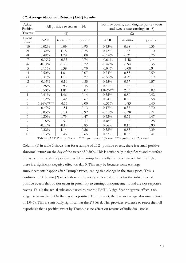
6.2. Average Abnormal Returns (AAR) Results

AAR: Positive Tweets

All positive tweets (n = 24) Positive tweets, excluding response tweets

and tweets near earnings (n=8)

(1) (2)

Event time

AAR t-statistic p-value AAR t-statistic p-value

-10 0.02% 0.09 0.93 0.43% 0.98 0.33

-9 0.32% 1.15 0.25 0.72% 1.63 0.10

-8 0.49% 1.78 0.08 -0.14% -0.31 0.76

-7 -0.09% -0.33 0.74 -0.66% -1.48 0.14

-6 -0.34% -1.22 0.22 -0.42% -0.94 0.35

-5 0.11% 0.39 0.70 -0.04% -0.08 0.94

-4 0.50% 1.81 0.07 0.24% 0.53 0.59

-3 0.31% 1.11 0.27 -0.58% -1.31 0.19

-2 -0.05% -0.19 0.85 0.25% 0.57 0.57

-1 0.26% 0.93 0.35 0.61% 1.38 0.17

0 0.50% 1.81 0.07 1.04%*** 2.36 0.02

1 0.41% 1.46 0.14 0.35% 0.80 0.42

2 0.12% 0.42 0.67 0.24% 0.55 0.58

3 -1.26%**** -4.53 0.00 -0.37% -0.83 0.40

4 -0.42% -1.51 0.13 0.17% 0.38 0.70

5 0.03% 0.10 0.92 -0.17% -0.38 0.71

6 0.20% 0.73 0.47 0.32% 0.72 0.47

7 0.16% 0.57 0.57 0.48% 1.08 0.28

8 -0.05% -0.19 0.85 0.06% 0.13 0.90

9 0.32% 1.14 0.26 0.38% 0.85 0.39

10 0.13% 0.45 0.65 0.37% 0.83 0.41 Table 2: AAR Positive Tweets ****significant at 1% level, ***significant at 2% level

Column (1) in table 2 shows that for a sample of all 24 positive tweets, there is a small positive

abnormal return on the day of the tweet of 0.50%. This is statistically insignificant and therefore

it may be inferred that a positive tweet by Trump has no effect on the market. Interestingly,

there is a significant negative effect on day 3. This may be because some earnings

announcements happen after Trump’s tweet, leading to a change in the stock price. This is

confirmed in Column (2) which shows the average abnormal returns for the subsample of

positive tweets that do not occur in proximity to earnings announcements and are not response

tweets. This is the actual subsample used to test the EMH. A significant negative effect is no

longer seen on day 3. On the day of a positive Trump tweet, there is an average abnormal return

of 1.04%. This is statistically significant at the 2% level. This provides evidence to reject the null

hypothesis that a positive tweet by Trump has no effect on returns of individual stocks.

19

AAR: Negative Tweets

All negative tweets (n=20) Negative tweets, excluding response

tweets and tweets near earnings (n=16)

(1) (2)

Event time AAR t-statistic p-value AAR t-statistic p-value

-10 -0.15% -0.52 0.60 -0.11% -0.38 0.70

-9 -0.22% -0.77 0.44 -0.23% -0.78 0.43

-8 -0.10% -0.35 0.72 0.14% 0.49 0.62

-7 0.02% 0.07 0.94 -0.12% -0.41 0.68

-6 -0.09% -0.33 0.74 -0.08% -0.28 0.78

-5 -0.32% -1.12 0.26 -0.22% -0.77 0.44

-4 -0.29% -1.02 0.31 -0.29% -1.00 0.32

-3 0.07% 0.24 0.81 0.28% 0.98 0.33

-2 -0.31% -1.11 0.27 -0.28% -0.96 0.34

-1 -0.22% -0.77 0.44 -0.21% -0.72 0.47

0 -0.31% -1.11 0.27 -0.85%**** -2.93 0.00

1 0.03% 0.10 0.92 -0.20% -0.67 0.50

2 0.20% 0.71 0.48 0.21% 0.71 0.48

3 -0.17% -0.60 0.06 -0.56% -1.93 0.06

4 0.40% 1.43 0.15 0.46% 1.59 0.11

5 -0.12% -0.41 0.68 -0.02% -0.05 0.96

6 -0.05% -0.19 0.85 0.30% 1.03 0.30

7 -0.02% -0.06 0.95 -0.17% -0.59 0.55

8 -0.21% -0.73 0.46 -0.38% -1.32 0.19

9 0.18% 0.65 0.51 0.19% 0.65 0.52

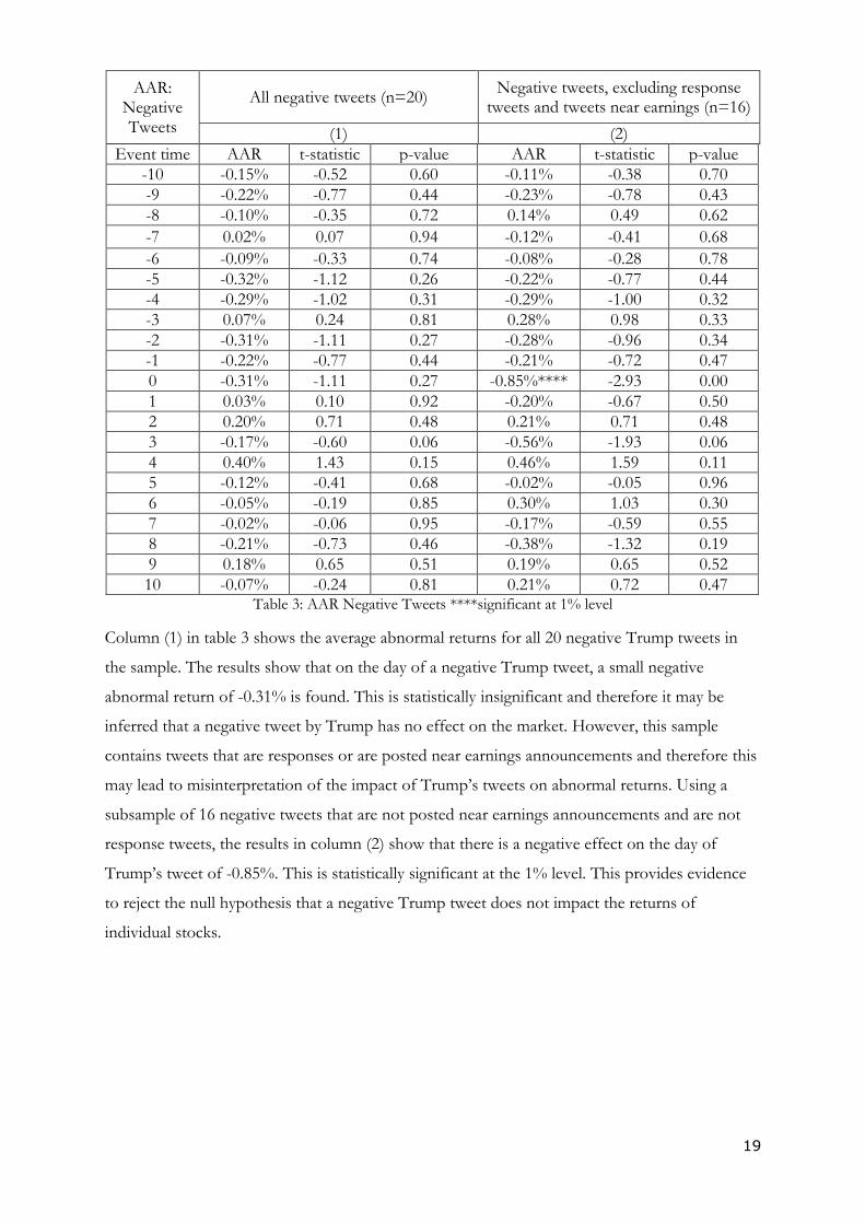
10 -0.07% -0.24 0.81 0.21% 0.72 0.47 Table 3: AAR Negative Tweets ****significant at 1% level

Column (1) in table 3 shows the average abnormal returns for all 20 negative Trump tweets in

the sample. The results show that on the day of a negative Trump tweet, a small negative

abnormal return of -0.31% is found. This is statistically insignificant and therefore it may be

inferred that a negative tweet by Trump has no effect on the market. However, this sample

contains tweets that are responses or are posted near earnings announcements and therefore this

may lead to misinterpretation of the impact of Trump’s tweets on abnormal returns. Using a

subsample of 16 negative tweets that are not posted near earnings announcements and are not

response tweets, the results in column (2) show that there is a negative effect on the day of

Trump’s tweet of -0.85%. This is statistically significant at the 1% level. This provides evidence

to reject the null hypothesis that a negative Trump tweet does not impact the returns of

individual stocks.

20

Figure 3: Average abnormal returns for positive and negative tweets

Figure 3 shows that that for positive tweets, on event day 0, there is a spike in abnormal returns

of 1%. For negative tweets there is a negative spike down to -0.85%. Interestingly, on day 2,

AARs return to pre-event levels. This suggests that the markets takes 2 days to adjust to new

information and therefore is inefficient. This will be analysed formally through CAAR.

Overall, the AAR results show that the null hypothesis of no impact of Trump’s tweets on AAR

can be rejected. As a result, the EMH can be tested by analysing the CAAR.

6.3. Cumulative Average Abnormal Return (CAAR)

CAAR: Negative &

Positive Tweets

Negative tweets, excluding response tweets and tweets near earnings

(n=16)

Positive tweets, excluding response tweets and tweets near earnings

(n=8)

(1) (2)

Event window CAAR t-statistic p-value CAAR t-statistic p-value

(-10,-1) -1.12% -1.22 0.22 0.43% 0.31 0.76

(0,1) -1.05%*** -2.55 0.01 1.40%** 2.23 0.03

(0,2) -0.84%* -1.67 0.05 1.64%** 2.14 0.03

(0,3) -1.40%*** -2.41 0.02 1.27% 1.44 0.15

(0,4) -0.94% -1.45 0.15 1.44% 1.46 0.15

(0,5) -0.96% -1.34 0.18 1.27% 1.18 0.24

(-10,10) -1.93% -1.45 0.15 3.30% 1.63 0.10 Table 4: ***Significant at 2% level, **Significant at 5% level, *Significant at 10% level

Column (1) in table 4 shows the CAAR of a subsample of 16 negative tweets that do not include

responses or earnings. There is a CAAR of -1.12% in the (-10,-1) pre-event period but this is

statistically insignificant which means that results are not contaminated by preceding events.

Looking across the whole 21-day sample, we find that there is a negative impact of -1.93% but

-1.00%

-0.50%

0.00%

0.50%

1.00%

1.50%

-10 -9 -8 -7 -6 -5 -4 -3 -2 -1 0 1 2 3 4 5 6 7 8 9 10

Aver

age

Ab

no

rmal

Ret

urn

Event Day

Average Abnormal Returns

Positive Tweet Negative Tweet

21

this is statistically insignificant so there seems to be no long-term impact of Trump’s tweets. The

immediate impact of a negative tweet is a negative return on average across stocks. This is shown

by the event window (0,1). There is an impact of -1.05% on average across the day of the tweet

and the day after the tweet. This is statistically significant at the 2% level. There is a significant

weaker negative effect of -0.84% for the (0,2) event window. Interestingly, the (0,3) event

window CAAR shows that there is a stronger negative effect of -1.40%, 3 trading days after the

tweet is made and this is statistically significant at the 2% level. A possible reason for this is that

Donald Trump’s tweets are released by the media a couple of days after he tweets, therefore the

effect may be delayed. Four trading days after the tweet, there is no longer an effect of Trump’s

tweets as the CAARs are no longer statistically significant. This means that the market has

adjusted. This is inconsistent with the semi-strong form of EMH, as new information is not

incorporated rapidly into the market.

Column (2) shows the results for a subsample of 8 positive tweets that are not response tweets

and do not occur near earnings announcements. There is a CAAR of 0.43% in the pre-tweet

period but this is statistically insignificant. Similarly to negative Trump tweets, there is no long-

term impact on the market. There is an significant immediate impact of 1.40% for the (0,1) event

window. Looking at the (0,2) event window, there is a stronger positive effect of 1.64% which is

statistically significant at the 5% level. The (0,3) event window shows that there is a positive

effect 3 trading days after the tweet is made but this is not statistically significant. Unlike negative

Trump tweets, on day 3, there is not a strong effect. This may contradict the initial suggestion

that the media is delayed in releasing information about Trump tweets. However, usually the

media only highlight negative Trump content. Therefore, this abides by the results, as negative

Trump tweets would receive more media coverage whereas positive tweets would not.10

Overall, the CAARs for both positive and negative tweets provide enough evidence to reject the

null hypothesis that markets are efficient as the market does not incorporate new information

instantly.

10 Pew Research Centre finds that 62% of media coverage on Trump is negative and only 5% is positive. Therefore, it may be argued that only negative tweets receive media coverage and positive tweets do not. This is why we see a stronger effect on day 3 for negative tweets relative to positive tweets.

22

7. Results: Testing for Attention-Based Investing

7.1. Average Abnormal Trading Volume (AAV) Results

AAV: Positive & Negative

Tweets

Positive & Negative tweets, excluding response tweets and tweets near earnings

(n = 24)

(1)

Event time AAV t-statistic p-value

-5 -9.11% -0.64 0.53

-4 -1.72% -0.12 0.90

-3 -8.78% -0.61 0.54

-2 -10.49% -0.73 0.46

-1 21.80% 1.52 0.13

0 43.57%**** 3.04 0.00

1 17.29% 1.21 0.23

2 -10.39% -0.73 0.47

3 -5.40% -0.38 0.71

4 8.52% 0.59 0.55

5 6.06% 0.42 0.67 Table 5: T-statistics are in parentheses. ****Significant at 1% level

A subsample of 8 positive and 16 negative tweets that do not occur near earnings

announcements and are not response tweets are used. Table 5 shows that on day 0, there is a

spike in abnormal trading volume of 43.57%. This is statistically significant at the 1% level.

However, after day 0, abnormal trading volumes are statistically insignificant. This implies that

Trump’s tweets do generate investor attention. Findings are consistent with the attention-based

investing hypothesis if retail investors act upon the information and Google search activity

confirms this.

7.2. Google Search Activity:

Company Week -2 Week -1 Week 0 Week +1 Week +2

Ford 42 49 52 47 44

United Technologies 36 29 100 77 54

Rexnord 0 0 100 97 0

Softbank 0 8 60 23 8

Boeing 46 24 16 16 16

Lockheed Martin 36 35 100 71 24

General Motors 22 23 85 53 27

Toyota 38 39 100 63 50

Amazon 52 46 32 29 33

Comcast 40 59 69 46 58

American Airlines 23 9 14 11 9

Facebook 53 52 61 65 53

CBS 63 56 95 69 94

Wells Fargo 45 53 59 49 43

Disney 68 56 53 47 41

J.P. Morgan 49 37 87 79 74

Average 38 36 68 53 53

Table 6: These values are the relative number of searches for each company during the period October 2016 to February 2018

23

On the week of the tweet, Google Trends finds that Trump’s tweets lead to an increase in the

search volume index from 36 in the previous week to 68 on average. A week after the event

week, the Google search activity begins to fall. This is consistent with attention-based buying as

investors only draw attention to stocks mentioned by Trump for the event week. After this,

investor attention is diverted away from these stocks.

8. Discussion:

8.1. General Analysis

This study finds that Trump can affect financial markets with his tweets. The effect of a positive

and negative tweet on abnormal returns is statistically and economically significant as the effect

on returns usually follows the sentiment of the tweet (a positive tweet leads to positive abnormal

returns). Interestingly, a positive tweet by Trump has more of an effect than a negative tweet on

the market. This contrasts from Ge et al. (2017) who find no difference in the effect of a

negative and positive tweet. A possible reason for this is that Trump’s company-specific tweets

are usually very negative and therefore positive tweets about companies are unexpected and

therefore lead to higher returns. Another reason for this may be that the positive tweet

subsample is smaller than the negative tweet subsample and therefore this may limit

interpretation. The market generally takes 2 to 3 trading days to incorporate the information

contained in these tweets and therefore the findings are inconsistent with the semi-strong form

of EMH. This is in line with studies by Born et al. (2017) and Ge et al. (2017). A key

contribution of this study is attention-based investing. Retail investors in particular tend to focus

on stocks mentioned by Trump and therefore do not consider all available information.

Contrastingly, Born et al. (2017) finds noise trading as the reason for market inefficiencies,

whereas Ge et al. (2017) do not provide a reason for observed market inefficiencies.

A real-world implication of this study is that trading strategies can be devised so that when

Trump tweets positively (negatively) an investor can short (buy) the stock and then exit their

position after 2 or 3 trading days. However, this may depend upon broker or transaction costs as

abnormal returns may not be high enough to cover this. Therefore, retail investors may not be

able to devise profitable strategies based upon Trump’s tweets. Nonetheless, institutional

investors, who can benefit from lower transaction costs, may be able to profit from these

announcements and devise trading strategies.

24

8.2. Justifications

EMH states that it is impossible to beat the market if markets are efficient. This event study

shows that the markets are possible to beat. However, if transaction costs are incorporated, there

may be a possibility that markets are actually efficient as the abnormal returns seen are low.

Nevertheless, there are now many brokers that charge various commissions. For instance, some

brokers offer flat rates per trade whereas others charge a monthly rate. Statistics for average

transaction costs in the US are difficult to obtain and therefore, it is unclear how to include

transaction costs into an event study. As a result, similar to other event studies11, transaction

costs are disregarded and focus is kept on the informational efficiency of markets.

8.3. Limitations

The small sample size for positive tweets limits interpretation. This is because most positive

tweets by Trump are response tweets, simply thanking companies for abiding by his policies. The

sample size in this study is 24 and this is an enlargement of previous work on the impact of

Trump’s tweets on financial markets. However, a larger sample size would improve this analysis.

Additionally, it could be argued that Google search activity is limited in its interpretation as the

data is indexed and is found on a weekly basis. On the other hand, this paper incorporates

trading volume in order to complement the result of Google Search Activity. A possible

limitation of event studies is that some preceding events may not be accounted for. However, to

minimise this limitation, this study excludes tweets that occur during earnings and company

announcements. This reduces the chance that preceding events drive the impact of Trump’s

tweets.

9. Conclusion

This paper finds that positive and negative Trump tweets move stock prices and lead to

significant abnormal returns. These effects last 2-3 trading days, which implies that the market is

inefficient. These findings suggest that Donald Trump does indeed use Twitter as a strategic tool

to influence the stock price and hence the actions of target companies. A key strength of this

paper is the new insight it adds in the form of attention-based buying. Transitory increases in

trading volume and Google search activity implies that Trump catches the attention of retail

investors who do not consider all available information.

Future research could innovate a way of incorporating transaction costs to make results more

robust and devise profitable trading strategies for retail and institutional investors. In order to

11 All studies mentioned in the literature review disregard transaction costs including Ge et al. (2017) and Born et al. (2017).

25

increase the accuracy of results, researchers could increase the sample size by analysing tweets at

the end of Trump’s presidential term. This would provide results that are more reliable. A bigger

sample size also means that specific industries could be analysed. For instance, some industries

that rely heavily on government contracts (such as defence) may be more susceptible to Trump’s

tweets. Furthermore, as Twitter rises in popularity, the effect of celebrities and other politicians

on financial markets could be analysed. Recently, Kylie Jenner tweeted negatively about Snap Co.

and this lead to a decrease in its stock market value by £1 billion. This shows that with a large

follower base, celebrities and politicians can affect organisations for the better or the worse. As

result, regulators may want to consider scrutinising the effect of Twitter on financial markets

more critically in the future.

26

10. Bibliography

Ball, R. and Brown, P. (1968). An Empirical Evaluation of Accounting Income Numbers. Journal of Accounting Research, 6(2). Barber, B. and Odean, T. (2005). All that Glitters: The Effect of Attention and News on the Buying Behavior of Individual and Institutional Investors. Review of Financial Studies, 21(2), 785-818. Bernard, V. and Thomas, J. (1989). Post-Earnings-Announcement Drift: Delayed Price Response or Risk Premium?. Journal of Accounting Research, 27. Born, J., Myers, D. and Clark, W. (2017). Trump tweets and the efficient Market Hypothesis. Algorithmic Finance, 6(3-4), pp.103-109. Brown, B. (2017). Trump Twitter Archive. Accessed 7 November 2017. Available at: http://www.trumptwitterarchive.com. Brown, S. and Warner, J. (1980). Measuring Security Price Performance. Journal of Financial Economics, 8(3), pp.205-258. Brown, S. and Warner, J. (1985). Using Daily Stock Returns: The Case of Event Studies. Journal of Financial Economics, 14(1), pp.3-31. Campbell, C. and Wasley, C. (1996). Measuring abnormal daily trading volume for samples of NYSE/ASE and NASDAQ securities using parametric and nonparametric test statistics. Review of Quantitative Finance and Accounting, 6(3), pp.309-326. Charest, G. (1978). Split information, stock returns and market efficiency-I. Journal of Financial Economics, 6(2-3), pp.265-296. Fama, E. (1965). The Behavior of Stock-Market Prices. The Journal of Business, 38(1). Fama, E., Fisher, L., Jensen, M. and Roll, R. (1969). The Adjustment of Stock Prices to New Information. International Economic Review, 10(1). Finance.yahoo.com. (2017). ^GSPC : Summary for S&P 500 - Yahoo Finance. Accessed 1 November 2017. Available at: https://finance.yahoo.com/quote/%5EGSPC?p=%5EGSPC. Gab, C., (2017). VADER Sentiment Analysis Explained - Data Meets Media. Data Meets Media. Accessed 10 November 2017. Available at: http://datameetsmedia.com/vader-sentiment-analysis-explained/. Ge, Q. and Wolfe, M. (2017). Stock Market Reactions to Presidential Social Media Usage: Evidence from Company-Specific Tweets. Hutto, C. and Gilbert, E. (2014). VADER: A Parsimonious Rule-based Model for Sentiment. Kilgore, T. (2017). Nordstrom recovers from Trump’s ‘Terrible!’ tweet in just 4 minutes. MarketWatch. Accessed 1 February 2018. Available at: https://www.marketwatch.com/story/nordstrom-recovers-from-trumps-terrible-tweet-in-just-4-minutes-2017-02-08.

27

Lexicon.ft.com. (2017). Beta Definition from Financial Times Lexicon. Accessed 10 November 2017. Available at: http://lexicon.ft.com/Term?term=beta. Lexicon.ft.com. (2017). Retail Investor Definition from Financial Times Lexicon. Accessed 10 November 2017. Available at: http://lexicon.ft.com/Term?term=retail-investor. Lexicon.ft.com. (2017). Share Split Definition from Financial Times Lexicon. Accessed 10 November 2017. Available at: http://lexicon.ft.com/Term?term=share-split. MacKinlay, C. (1997). Event Studies in Economics and Finance. Journal of Economic Literature 35(1). Malaver-Vojvodic, M. (2017). Measuring the Impact of President Donald Trump’s Tweets on the Mexican Peso/U.S. Dollar Exchange Rate. Mimeo, University of Ottawa. Mitchell, A., Gottfried, J., Stocking, G., Matsa, K. and Grieco, E. (2017). 3. A comparison to early coverage of past administrations. Pew Research Center's Journalism Project. Accessed 24 Apr. 2018. Available at: http://www.journalism.org/2017/10/02/a-comparison-to-early-coverage-of-past-administrations/ Peterson, P. (1989). Event studies: A review of Issues and Methodology. Quarterly Journal of Business and Economics 28(3). Ranco, G., Aleksovski, D., Caldarelli, G., Grčar, M. and Mozetič, I. (2015). The Effects of Twitter Sentiment on Stock Price Returns. PLOS ONE, 10(9). Statista. (2018). Leading global social networks 2018. Accessed 21 March 2018. Available at: https://www.statista.com/statistics/272014/global-social-networks-ranked-by-number-of-users/. Support.google.com. (2018). Trends Help. Accessed 10 February 2018. Available at: https://support.google.com/trends/?hl=en#topic=6248052. Technician. (2018). Technician - Real-time stock charts for mobile and web. Accessed 4 December 2017. Available at: http://technicianapp.com. Tetlock, P. (2007). Giving Content to Investor Sentiment: The Role of Media in the Stock Market. The Journal of Finance, 62(3), pp.1139-1168. Time. (2017). Meet the 25 Most Influential People on the Internet. [online] Available at: http://time.com/4815217/most-influential-people-internet/. Twlets. (2018). Accessed 1 November 2017. Available at: http://twlets.com. Wang, C. (2016). Lockheed Martin shares take another tumble after Trump tweet. CNBC. Available at: https://www.cnbc.com/2016/12/22/lockheed-martin-shares-take-another-tumble-after-trump-tweet.html. YouTube. (2016). Event Study Walkthrough in Excel. Accessed 1 November 2017. Available at: https://www.youtube.com/watch?v=McxSD1Vm9Xg. Yurieff, K. (2018). Snapchat stock loses $1.3 billion after Kylie Jenner tweet. CNNMoney. Accessed 30 March 2018. Available at: http://money.cnn.com/2018/02/22/technology/snapchat-update-kylie-jenner/index.html.

28

11. Appendices

11.1. Appendix A: Summary of Literature

Paper Announcement

type Time range

How long does the post-

announcement effect last?

Is the market

efficient? Sample size

Fama, Fisher,

Jensen and Roll (1969)

Stock splits 1927-1959 0 months Yes 940 stock splits

Ball and Brown (1968)

Annual earnings announcements

1944-1966 6 months No 75 firms

Bernard and Thomas (1989)

Quarterly earnings announcements

1974-1986 60 days No 84,792 firm-

quarters of data

Charest (1978)

Dividend policy 1947-1967 3 months No

1720 dividend

announcements

Tetlock (2007)

Newspaper column

1984-1999 2 days No 30 firms

Ranco et al. (2015)

Tweets 2013-2014 10 days No 100,000 tweets

Malaver and Vojvodic

(2017) Trump’s tweets 2015-2017 N/A N/A 7,429 tweets

Born et al. (2017)

Trump’s tweets 2016 5 trading days No 15 tweets

Ge et al. (2017)

Trump’s tweets 2016-2017 2 trading days No 48 tweets – 18 of

which are informative

29

11.2. Appendix B: Earnings Announcement Dates

Earnings Dates 2017 Q4 2016 Q1 2017 Q2 2017 Q3 2017 Q4 2017 Q1 2018

Ford 01/26/2017 04/27/2017 07/26/2017 10/26/2017 24/01/2018 04/25/2018

General Motors 02/07/2017 04/28/2017 07/25/2017 10/24/2017 02/06/2018 04/26/2018

Toyota 02/06/2017 05/10/2017 08/04/2017 11/07/2017 02/06/2018 05/09/2018

Fiat Chrysler 01/26/2017 04/26/2017 07/27/2017 10/24/2017 01/25/2018 04/26/2018

Walmart 02/21/2017 05/17/2017 08/17/2017 11/16/2017 02/20/2018 05/17/2018

Intel 01/26/2017 04/27/2017 07/27/2017 10/26/2017 01/25/2018 04/26/2018

Nordstrom 02/23/2017 05/11/2017 08/10/2017 11/09/2017 03/01/2018 05/10/2018

Exxon 01/31/2017 04/28/2017 07/28/2017 10/27/2017 02/02/2018 04/27/2018

Rexnord 02/02/2017 05/18/2017 08/02/2017 11/01/2017 01/31/2018 05/16/2018

Amazon 02/02/2017 04/27/2017 07/27/2017 10/26/2017 02/01/2018 04/26/2018

Comcast 01/26/2017 04/27/2017 07/27/2017 10/26/2017 01/24/2018 04/25/2018

Corning 01/24/2017 04/25/2017 07/26/2017 10/24/2017 01/30/2018 04/24/2018

Merck 02/02/2017 05/02/2017 07/28/2017 10/27/2017 02/02/2018 05/01/2018

Pfizer 01/31/2017 05/02/2017 08/01/2017 10/31/2017 01/30/2018 05/01/2018

CBS 02/15/2017 05/04/2017 08/07/2017 11/02/2017 02/15/2018 05/03/2018

American Airlines 01/27/2016 04/27/2017 07/28/2017 10/26/2017 01/25/2018 04/26/2018

Facebook 02/03/2017 05/03/2017 07/26/2017 11/01/2017 01/31/2018 05/02/2018

Broadcom 12/08/2016 03/01/2017 06/01/2017 08/24/2017 12/06/2017 03/15/2018

Wells Fargo 01/13/2017 04/13/2017 06/14/2017 10/13/2017 01/12/2018 03/08/2018

Apple 10/21/2016 01/31/2017 05/02/2017 08/01/2017 11/02/2017 02/01/2018

Disney 11/10/2016 02/07/2017 05/09/2017 08/08/2017 11/09/2017 02/06/2018

J.P. Morgan 01/13/2017 04/13/2017 07/14/2017 10/12/2017 01/12/2018 04/12/2018

These dates are used in order to determine whether Trump’s tweets occur during earnings announcements. The bolded dates highlight earnings announcements that occur in proximity to Trump’s

tweets.

30

11.3. Appendix C: Positive and Negative Tweets

Positive Tweets Sample:

Company Ticker Date Time

Does The Tweet

Occur Near Earnings

Date?

Is The Tweet A Response To A

Company Announcement?

Subject Of The Tweet

Ford F 11/17/2016 9:51 PM No No

Announcing that Ford are keeping plant in US not

Mexico

United Technologies UTC 11/24/2016 10:12 AM No No Working on Carrier

to stay in US

United Technologies* UTC 11/29/2016 10: 40 PM No Yes Responding to UTC

staying in US

Softbank SFTBK 12/06/2016 2:10 PM No No

Announcing Softbank CEO

agreeing to invest in US

Boeing BOE 12/22/2016 5:26 PM No No Asked BOE to price

out LMT

Ford F 01/04/2017 8:19 AM No No Announcing ford

scrapping new plant in Mexico

Fiat Chrysler* FCAU 01/09/2017 9:14 AM No Yes Responding to

FCAU investment

General Motors* GM 01/17/2017 12:55 PM No Yes Thank you for

investment

Walmart* WMT 01/17/2017 12:55 PM No Yes Thank you for

investment

General Motors* GM 01/24/2017 7:47 PM No Yes Great meeting with

CEO

Ford* F 01/24/2017 7:47 PM Yes Yes Great meeting with

CEO

Intel* INTC 02/08/2017 2:22 PM No Yes Thank you for

investment

Exxon* XOM 03/06/2017 4:19 PM No Yes Thank you for

investment

Corning* GLW 07/21/2017 10:31 PM No Yes Thank you for

investment & new jobs

Merck* MRK 07/21/2017 10:31 PM No Yes Thank you for

investment & new jobs

Pfizer* PFE 07/21/2017 10:31 PM No Yes Thank you for

investment & new jobs

American Airlines AAL 09/22/2017 12:54 PM No No Helping with flights during the hurricane

Broadcom** AVGO 11/02/2017 2:58 PM No Yes Thank you for

investment

Toyota* TM 01/10/2018 6:37 PM No Yes Thank you for

investment and new jobs

31

Apple* AAPL 01/17/2018 06:28 PM No Yes Thank you for

investment and new jobs

Fiat Chrysler* FCAU 01/17/2018 6:32 PM No Yes Thank you for moving from Mexico to US

Disney DIS 01/24/2018 6:58 AM No No Good progress in

US

J.P. Morgan JPM 01/24/2018 6:58 AM No No Good progress in

US

Fiat Chrysler* FCAU 01/28/2018 8:18 AM Yes Yes Thank you for moving from Mexico to US

*Excluded tweets as they either are response tweets or occur near earnings announcements **Broadcom announced bid for Qualcomm and this tweet is excluded as a result

Negative tweets sample:

Company Ticker Date Time

Does The Tweet Occur

Near Earnings Date?

Is The Tweet A Response To A

Company Announcement?

Subject Of The Tweet

Rexnord RXN 12/02/2016 10:06 PM No No Worker negligence

Boeing BOE 12/06/2016 8:52 AM No No Boeing prices are out of

control

Lockheed Martin LMT 12/12/2016 2:26 PM No No F-35 programme out of

control

Lockheed Martin LMT 12/22/2016 5:26 PM No No Asked Boeing To Price

out LMT

General Motors GM 01/03/2017 7:30 AM No No Threating large border

taxes

Toyota TM 01/05/2017 1:14 PM No No Threating large border

taxes

Nordstrom* JWN 02/08/2017 10:51 AM No Yes

Frustration at Nordstrom

discontinuing Ivanka Trump’s clothing line

Rexnord RXN 05/07/2017 5:58 PM No No Threatening to tax products sold in us

Amazon AMZ 06/28/2017 8:06 AM No No Amazon should pay

internet taxes

Comcast CMCSA 07/01/2017 7:59 AM No No Fake news

CBS* CBS 08/07/2017 6:18 AM Yes No Fake news

Merck* MRK 08/14/2017 7:54 AM Yes No ‘Rip-off’ drug prices

Amazon AMZ 08/16/2017 5:12 AM No No Amazon damaging tax-

paying retailers

Facebook FB 09/27/2017 8:36 AM No No Suggesting collusion between FB and CBS

CBS CBS 10/17/2017 4:51 PM No No Fake news

Facebook FB 10/21/2017 3:06 PM No No Fake news

CBS CBS 10/21/2017 3:06 PM No No Fake news

Comcast* CMCSA 11/29/2017 7:16 AM No Yes Fake news

Wells Fargo WF 12/08/2017 10:18 AM No No Threating tougher

penalties for behaviour

Amazon AMZ 12/29/2017 8:04 AM No No Amazon should pay

more to US Post Office

*Excluded tweets as they either are response tweets or occur near earnings announcements

32

11.4. Appendix D: Google Search Terms

Company Ticker Search Term Used

Ford F ‘Ford stock price’

United Technologies UTC ‘United Technologies stock price’

Rexnord* RXN ‘Rexnord stock’

Softbank SFTBK ‘Softbank stock price’

Boeing BOE ‘Boeing stock price’

Lockheed Martin LMT ‘Lockheed Martin stock price’

General Motors GM ‘General Motors stock price’

Toyota TM ‘Toyota stock price’

Amazon AMZ ‘Amazon stock price’

Comcast CMCSA ‘Comcast stock price’

American Airlines AA ‘American Airlines stock price’

Facebook FB ‘Facebook stock price’

CBS CBS ‘CBS stock price’

Wells Fargo WF ‘Wells Fargo stock price’

Disney DIS ‘Disney stock price’

J.P. Morgan JPM ‘JP Morgan stock price’

*’Rexnord stock’ is used as the search term instead of ‘Rexnord stock price’ as there were not enough searches for Rexnord stock price