The impact of endothermy on the climatic niche evolution

Articleshttps://doi.org/10.1038/s41559-017-0451-9

© 2018 Macmillan Publishers Limited, part of Springer Nature. All rights reserved.

The impact of endothermy on the climatic niche evolution and the distribution of vertebrate diversityJonathan Rolland 1,2,3*, Daniele Silvestro 1,2,4,5, Dolph Schluter3, Antoine Guisan6,7, Olivier Broennimann6,7 and Nicolas Salamin1,2

1Department of Computational Biology, Biophore, University of Lausanne, Lausanne, Switzerland. 2Swiss Institute of Bioinformatics, Quartier Sorge, Lausanne, Switzerland. 3Department of Zoology, University of British Columbia, Vancouver, Canada. 4Department of Biological and Environmental Sciences, University of Gothenburg, Gothenburg, Sweden. 5Gothenburg Global Biodiversity Centre, Gothenburg, Sweden. 6Department of Ecology and Evolution, Biophore, University of Lausanne, Lausanne, Switzerland. 7Institute of Earth Surface Dynamics, Geopolis, University of Lausanne, 1015 Lausanne, Switzerland. *e-mail: [email protected]

SUPPLEMENTARY INFORMATION

In the format provided by the authors and unedited.

NATuRe ecOlOGy & evOluTiON | www.nature.com/natecolevol

https://doi.org/10.1038/s41559-017-0451-9

http://orcid.org/0000-0002-7141-0870

http://orcid.org/0000-0003-0100-0961

mailto:[email protected]

http://www.nature.com/natecolevol

Supplementary methods and results 31

32

Simulations of the ancestral states and quality of the estimates 33

We simulated a set of true ancestral states and we then tested whether our method could recover 34

accurately these states only with partial information (present day data and few/no fossils). These 35

tests are described in details in the supplementary material of Silvestro et al. 2017 52 (the following 36

text has been modified from 52): For each simulation, we generated a complete phylogenetic tree 37

(extinct and extant taxa) under a constant rate of birth-death with 100 extant tips (using the 38

sim.bd.taxa function with parameters: speciation rate (λ) = 0.4, and extinction rate (µ) = 0.2, in the 39

R package TreePar53). The number of fossils simulated on the tree was defined by a Poisson 40

distribution with expected number of occurrences set to 1, 5, and 20. Additional simulations were 41

also run without any fossils for comparison. The simulation under the model presented here 42

correspond to a constant rate of evolution σ2 drawn from a gamma distribution Γ(2, 5), and no 43

phenotypic trend (µ0 = 0). We simulated 100 data sets under each scenario (i.e. number of fossils 44

= 0, 1, 5, and 20). We analyzed each simulated dataset to estimate the rate parameters of the 45

Brownian Motion model (σ2) and the ancestral states. Each dataset was run for 500,000 MCMC 46

generations, sampling every 500 steps. We summarized the results in two ways. First, we 47

numerically quantified the overall accuracy of the σ2 estimate across all simulations using the mean 48

absolute percentage error (MAPE): 49

50

where j is the simulation number, is the estimated rate at branch i, and is the true rate at 51

branch i, and N is the number of branches in the tree. Secondly, we calculated the coefficient of 52

across all simulations using di↵erent summary statistics for each set of parameters. The the

BM rate parameters (�2) we calculated the mean absolute percentage error (MAPE),

defined as:

MAPEj(�2) =

1

N

NX

i=1

|�̂2

i � �

2

i |�

2

i

!(2)

where j is the simulation number, �̂2

i is the estimated rate at branch i, �2

i is the true rate

at branch i, and N is the number of branches in the tree. Because the trend parameter can

take both negative and positive values, we used the mean absolute error (MAE) to quantify

the accuracy of its estimates:

MAEj(µ0

) =1

N

NX

i=1

⇣|µ̂i

0

� µ

i0

|⌘

(3)

where µ̂

i0

is the estimated trend at branch i and µ

i0

is the true trend at branch i. We

quantified the accuracy of the ancestral state estimates in terms of coe�cient of

determination (R2) between the true and the estimated values. These summary statistics

were computed for each simulation scenario (across 100 replicates) and are provided in

Figs. S2 and S3.

Finally, we assessed the ability of the BDMCMC algorithm to identify the correct

BM model of evolution in terms of number of shifts in rate and trend parameters. We

calculated the mean probability estimated for models with di↵erent number of rate shifts

(K�2 ranging from 0 to 4) and shifts in trends (Kµ0 ranging from 0 to 4). Note that K = 0

indicates a model with constant rate and/or trend parameter across branches. The

estimated posterior probability of a given number of rate shifts was obtained from the

frequency at which that model was sampled during the MCMC (Stephens, 2000). We

averaged these probabilities across 100 simulations under each scenario. We additionally

calculated the percentage of simulations in which each model was selected as the best

7

not peer-reviewed) is the author/funder. All rights reserved. No reuse allowed without permission. The copyright holder for this preprint (which was. http://dx.doi.org/10.1101/178111doi: bioRxiv preprint first posted online Aug. 18, 2017;



defined as:

MAPEj(�2) =

1

N

NX

i=1

|�̂2

i � �

2

i |�

2

i

!(2)



i is the true rate




MAEj(µ0

) =1

N

NX

i=1

⇣|µ̂i

0

� µ

i0

|⌘

(3)

where µ̂

i0


i0





Figs. S2 and S3.










7




defined as:

MAPEj(�2) =

1

N

NX

i=1

|�̂2

i � �

2

i |�

2

i

!(2)



i is the true rate




MAEj(µ0

) =1

N

NX

i=1

⇣|µ̂i

0

� µ

i0

|⌘

(3)

where µ̂

i0


i0





Figs. S2 and S3.










7


determination (R2) between the true and the estimated ancestral states. These analyses showed that 53

our method is not biased (Supplementary Figure 8) and yields accurate estimations of ancestral 54

states (Supplementary Figure 9). Additional test on the performance of the method are described 55

in Silvestro et al. 52. The code used to run these simulations is available at: 56

https://github.com/dsilvestro/fossilBM. 57

58

Robustness of the results 59

60

To verify that our results were not affected by methodological biases, we ran a series of robustness 61

tests. 62

1. Niche evolution estimates might be artificially high in mammals and birds because there 63

is more fossil data in these groups, or if the fossil record is biased (e.g if tropical 64

occurrences were less likely to be recorded in the fossil record). We ran all of the analyses 65

again without the fossils and found that niche evolution remained faster in 66

endotherms (Supplementary Figure 2). This latter result ensure that the main results of our 67

study will hold even if fossil occurrences might not reflect the true ancestral latitude of the 68

clades, and if fossils are misplaced on the tree (e.g. including changes in taxonomy between 69

the fossil record and the phylogeny). 70

2. Niche evolution estimates might be artificially high in mammals and birds because these 71

two groups have larger phylogenies. We ran all of the analyses again using pruned trees 72

for each group and found that niche evolution remained faster in endotherms 73

(Supplementary Figure 2). 74

3. Niche evolution estimates might be artificially low in amphibians and squamates because 75

they are older groups. We tested for a relationship between the estimates of niche evolution 76

rates in the 20 main orders (in birds and mammals) or families (in amphibians and 77

squamates) and their age and did not observe a significant relationship (Supplementary 78

Figure 6), which suggests that our results are not biased in this respect. 79

4. Niche evolution estimates might be artificially high in mammals and birds because of our 80

evolution model. We tested whether similar niche evolution estimates could be obtained 81

when applying Brownian motion (BM) and Ornstein-Uhlenbeck (OU) models (using the 82

fitContinuous R function in the geiger package). We obtained mean temperatures for each 83

species for which we had occurrence data points (GBIF), spatial distribution data (IUCN) 84

and mean annual temperature climatic layer data (BIO1, WorldClim), and we estimated 85

the rate of temperature evolution along the phylogenies for the four groups. These results, 86

which do not include fossil information, confirmed our previous results in which 87

endotherms were shown to have a faster niche evolution rate (Supplementary Table 1). 88

5. Niche evolution estimates might be artificially high in birds because of migratory behavior. 89

It is difficult to describe with confidence the distribution of migratory species, as their 90

occupancy area change across seasons. For birds, we estimated the niche evolution rate 91

based on the mean annual temperatures of both the breeding and wintering ranges (the 92

global distribution of each species without accounting for seasonal changes). This 93

simplification might affect our niche evolution reconstruction and we might have 94

underestimated the mean temperatures of migratory species; thus, we may have artificially 95

inflated the rate of niche evolution in birds. To test for this potential bias, we re-estimated 96

the rate of niche evolution using a BM model (using the fitContinuous R function in the 97

geiger package) that did not include fossil data but did include a phylogeny that only 98

contained sedentary species as well as the mean temperatures obtained for each species. 99

We also obtained migratory bird status data using the BirdLife International and 100

NatureServe databases (http://www.birdlife.org/). Following the method described in 101

Somveille et al.54, we considered a species to be migratory if it has at least one non-102

breeding season polygon or one breeding season polygon (see Rolland et al.55 for more 103

details). We found migratory data for 6,142 of the species in our dataset, and we removed 104

1,387 migratory species, thus retaining a total of 4,755 sedentary species. We obtained 105

comparable BM estimates between the sedentary birds (e.g., BM σ2= 9.05) and all birds 106

(e.g., BM σ2=14.84, Supplementary Table 1), suggesting that potential bias caused by using 107

mean annual temperatures does not affect our results and indicating that niche evolution 108

remains higher in birds than in the three other groups (Mammals BM σ2=2.92, Amphibians 109

BM σ2=1.01 and Squamates BM σ2=0.65, Table S1). 110

6. GBIF occurrence data points might be unevenly distributed inside the IUCN polygons and 111

lead to biased values of altitude, latitude and temperature. If the occurrence points inside 112

the polygons were geographically (or environmentally) clustered, we would expect to see 113

a mismatch between data extracted from polygons alone and data extracted from 114

occurrences points inside the polygons. We thus extracted the latitude, altitude and 115

temperature values for each species from polygons alone and we then tested if there was a 116

considerable difference with the same data obtained from occurrences inside the polygons. 117

We found no systematic bias in the values extracted with both approaches and an extremely 118

high association between these variables (for latitude: R2birds = 0.88, R2

mammals = 0.97, 119

R2amphibians = 0.99, R2

squamata = 0.99; for altitude: R2birds = 0.78, R2

mammals = 0.8, R2amphibians = 0.86, 120

R2squamata = 0.83; and for temperature: R2

birds = 0.82 , R2mammals = 0.91, R2

amphibians = 0.91, 121

R2squamata = 0.91; P<10-16 for all groups). These results suggest that occurrences data are not 122

strongly biased and represent accurately the variation of ecological conditions contained 123

inside polygons. 124

7. The temperature curve used in our study might be biased in the Neogene due to the 125

presence of ice volumes. Our paleo-temperature curve is based on the deep-sea benthic 126

foraminiferal oxygen-isotope δ18O (Zachos et al. 19). These estimates conflate temperature 127

and ice volume, which may be problematic when comparing greenhouse Eocene and 128

icehouse Neogene. We now run the analyses with two other Cenozoic curves from Cramer 129

et al. 2011 56 (based on formulas 7a and 7b in the supplementary information of the study) 130

that are based on the ratio Mg/Ca for the Cenozoic. In order to cover the 270 Myr of our 131

study, we did not change the temperature curve before 62.4 Myr, and the Cramer et al. 132

2011 56 curves were used after 62.4 Myr (we ran two independent analyses for the two 133

curves). We found no effect of these new curves on our results with faster rate of niche 134

evolution in birds and mammals compared to squamates and amphibians (birds= 0.86 or 135

0.64°C/Myr, respectively for the formulas 7a or 7b of Cramer et al. 2011 56, mammals= 136

0.70 or 0.52°C/Myr, amphibians= 0.37 or 0.31 °C/Myr, squamates= 0.40 or 0.33°C/Myr. 137

8. We also tested whether branches leading to nodes or tips informed by fossil or present-day 138

data were giving the same results as the whole phylogeny. This test permitted to test the 139

robustness of our phylogenetic approach. We found the same results with only branches 140

related to nodes informed by fossil or tips informed by field data, with higher rate of niche 141

evolution for endotherms than ectotherms (mean rate of niche evolution birds= 142

2.09°C/Myr, mammals= 2.37°C/Myr, amphibians= 0.56°C/Myr, squamates= 143

0.61°C/Myr). 144

145

Supplementary references 146

52. Silvestro D., Tejedor M. F., Serrano-Serrano M. L., Loiseau O., Rossier V., Rolland J., 147

Zizka A., Antonelli A. & Salamin N. Evolutionary history of New World monkeys 148

revealed by molecular and fossil data. BioRxiv (2017) (available online at 149

http://www.biorxiv.org/content/early/2017/08/18/178111.article-metrics ). 150

53. Stadler, T. Mammalian phylogeny reveals recent diversification rate shifts. Proc. Natl. 151

Acad. Sci. U.S.A. 108 , 6187-6192 (2011). 152

54. Somveille, M., Manica, A., Butchart, S. H. & Rodrigues, A. S. Mapping global diversity 153

patterns for migratory birds. PLOS ONE 8, e70907 (2013). 154

55. Rolland, J., Jiguet, F., Jønsson, K. A., Condamine, F. L. &Morlon, H. Settling down of 155

seasonal migrants promotes bird diversification. Proc. Biol. Sci. 281, 20140473 (2014). 156

56. Cramer, B. S., Miller, K. G., Barrett, P. J., & Wright, J. D. Late Cretaceous–Neogene trends 157

in deep ocean temperature and continental ice volume: Reconciling records of benthic 158

foraminiferal geochemistry (δ18O and Mg/Ca) with sea level history. J. Geophys. Res 159

Oceans. 116. (2011). 160

161

162

163

164

165

166

Supplementary Figure 1. Bayesian inference of ancestral states using a fossil-calibrated 167 Brownian motion model of evolution. The example shows an ultrametric tree with trait values 168 indicated by the size of the circles at the tips and at the internal nodes. The ancestral state of any 169 given internal node i is sampled directly from its joint posterior distribution through Gibbs 170 sampling. The joint posterior distribution of node i is a normal distribution obtained by combining 171 four normal distributions: three from the expectation of the Brownian motion with rate parameter 172 σ2 (ancestral node in dark blue and the two descendant values in purple and light blue) and one for 173 the prior assigned to the node (in red). The prior is either informative, i.e. when defined based on 174 fossil data, or non-informative with an arbitrary large variance if fossils are not available (see 175 "Fossils" and "Ancestral reconstruction of latitude and altitude" sections for more details). 176

177

Supplementary Figure 2. Robustness analysis. Niche evolution remains faster in endotherms 178 even when trees are pruned and fossil data are removed. The niche evolution of each group 179 was estimated based on four reconstructions: minimum and maximum latitude and minimum and 180 maximum altitude. These four analyses were run on trees of five different sizes for birds (3000, 181 1500, 1000, 500 and 100 tips), four different sizes for mammals (1500, 1000, 500 and 100 tips), 182 three different sizes for amphibians (1000, 500 and 100 tips), and two different sizes for squamates 183 (500 and 100 tips). Each reconstruction was replicated five times for each tree size, for a total of 184 5 x 4 x 14=280 reconstructions. We designed a pruning algorithm to remove randomly 185 monophyletic clades from the original tree (code available at 186 https://github.com/jonathanrolland/niche_evolution). This methodology allowed us to retain the 187 phylogenetic signal inside each group and was more conservative than randomly pruning 188 individual tips (rates of niche evolution were substantially higher when the tips were randomly 189 removed). In addition, to account for the potential effect of fossils in our results, we did not 190 consider fossil information in these robustness analyses. 191

192

0 500 1000 1500 2000 2500 3000

0.2

0.4

0.6

0.8

ntips

Med

ian

of th

e sp

eed

of n

iche

evo

lutio

n

0 500 1000 1500 2000 2500 3000

0.2

0.4

0.6

0.8

0 500 1000 1500 2000 2500 3000

0.2

0.4

0.6

0.8

0 500 1000 1500 2000 2500 3000

0.2

0.4

0.6

0.8

Med

ianofth

erateofn

icheevolution(°C

/Myr)

Number ofterminalbranchesinthephylogeny

193 Supplementary Figure 3. Avian (red) and mammalian (orange) species cover a wider range 194 of mean temperature, mean latitude and mean altitude than amphibian (green) and 195 squamate (blue) species. Violin plots were calculated using all of the species in each group. 196

-10 0 10 20 30

12

34

Mean temperature (°C)

0 10 20 30 40 50

12

34

Temperature range per species (°C)

-60 -40 -20 0 20 40 60

12

34

Mean latitude (°)

0 20 40 60 80 100 120 140

12

34

Latitude range per species (°)

0 1000 2000 3000 4000 5000 6000

12

34

Mean altitude (m)

0 2000 4000 6000 8000

12

34

Altitude range per species (m)

A

B

C

197

Supplementary Figure 4. Median rate of niche evolution for the 20 richest orders of birds 198 (red) and mammals (orange) and the 20 richest families of amphibians (green) and 199 squamates (blue). 200

0.5

1.0

1.5

2.0

2.5

3.0

Names of clades

Med

ian

of th

e sp

eed

of n

iche

evo

lutio

n (°

C/M

yr)

Med

ianofth

erateofn

icheevolution(°C

/Myr)

Names oftheclades

201 Supplementary Figure 5. Latitudinal diversity gradients of the groups that showed rapid 202 niche evolution. The vertical red line corresponds to the equator. 203

204

205

206

207

208

209

210

ANSERIFORMES

-60 -40 -20 0 20 40 60 80

05

15

PROCELLARIIFORMES

-60 -40 -20 0 20 40 60 80

010

20

LAGOMORPHA

-60 -40 -20 0 20 40 60 80

05

1015

CARNIVORA

-60 -40 -20 0 20 40 60 80

010

2030

MEGOPHRYIDAE

-60 -40 -20 0 20 40 60 80

04

812

BUFONIDAE

-60 -40 -20 0 20 40 60 80

05

15

NATRICIDAE

-60 -40 -20 0 20 40 60 80

05

15

ELAPIDAE

-60 -40 -20 0 20 40 60 80

04

8

Numberofspecies

Latitude Latitude

BIRDS

MAMMALS

AMPHIBIANS

SQUAMATES

211

Supplementary Figure 6. Robustness analysis. Niche evolution rates are not associated with 212 the age of the clades (orders and families). The rate of niche evolution was estimated for the 20 213 richest orders of birds (red) and mammals (orange) and the 20 richest families of amphibians 214 (green) and squamates (blue). The black line represents the regression of the linear model between 215 the rate of niche evolution and the age of the groups (P > 0.05). 216

217

218

219

220

221

222

223 224

20 40 60 80 100

0.5

1.0

1.5

2.0

2.5

Age of clades

Med

ian

of th

e sp

eed

of n

iche

evo

lutio

n (°

C/M

yr)

Ageofclades(Myr)

Med

ianofth

espeedofth

enicheevolution(°C

/Myr)

P >0.05

225

Supplementary Figure 7. Description of the procedure to obtain temperature for each node 226 of the phylogeny from both the reconstructions of latitude and altitude and the climatic grid 227 through time. 228 229 230 231 232 233 234 235 236 237 238 239

Rescaling allthevaluesofthe temperature grid withthedeltatemperaturebetween t andpresent

Altitude

Latitude

The firstgrid is calculated fromtemperature layers atpresent

Altitude

Latitude

+!Tt2+!Tt1

1

2

3

!!!!!

!!!!!

Majority!of!dispersal!!toward!the!poles!

Toward!the!equator!

Prop

or6o

n!of!descend

ants!!

dispersing!to

ward!the!po

les!

La6tude!of!the!ancestors!(°)!

!!!!!

!!!!!

!!!!!

Tempe

rature!(°C)!

!

A"

B" C" D" E"!!!!!!!!

K/T!boundary! EoceneDOligocene!!Transi6on!

Miocen!Clima6c!Op6mum!

Cretaceous! Cenozoic!

145 Myrs - 66 Myrs

0 20 40 60 80

0

0.25

0.5

0.75

1

66 Myrs - 33.9 Myrs

0 20 40 60 80

0

0.25

0.5

0.75

1

Pro

porti

on o

f lin

eage

s di

sper

sing

tow

ard

the

pole

s

33.9 Myrs - 15 Myrs

0 20 40 60 80

0

0.25

0.5

0.75

1

Pro

porti

on o

f lin

eage

s di

sper

sing

tow

ard

the

pole

s

15 Myrs - 0 Myrs

0 20 40 60 80

0

0.25

0.5

0.75

1

Pro

porti

on o

f lin

eage

s di

sper

sing

tow

ard

the

pole

s

145"–"66" 66","33.9" 33.9","15" 15","0"" Time"(Myr)"

!Tt2

t1t2

!Tt1

time present

Reconstruct altitude andlatitudepreferences onphylogenies

altitude

latitude

4 Determine the temperaturecorresponding tothe latitude-altitudecombination ofeach node forthegridbuilt attheage of thenode.

temperature

y1y2

y2

y1

x1 x2

Altitude

Latitudex1

x2

240 241 242 Supplementary Figure 8. Accuracy of parameter estimation summarized across 100 243 simulations. Mean absolute percentage errors (MAPE) are reported for the rate parameters (σ2, 244 panel A), and the coefficient of determination is used for ancestral states (R2, panel B, modified 245 from Figure S2 of Silvestro et al. 2017 52). 246 247

Scenario 1 Scenario 2 Scenario 3 Scenario 4 Scenario 5 Scenario 6

0.0

0.1

0.2

0.3

0.4

0.5

a) Rate parameters

MAP

E si

g2


0.0

0.1

0.2

0.3

0.4

0.5

b) Trend parameters

MAE

mu0


0.80

0.85

0.90

0.95

1.00

c) Ancestral states

R2

Ance

stra

l sta

tes

Figure S2: Accuracy of parameter estimation summarized across 100 simulations under sixsimulation settings (see Supplementary Methods). Mean absolute percentage errors (MAPE)are reported for the rate parameters (a; �2), Mean absolute errors (MAE) are used for thetrend parameters (b; µ

0

) and the coe�cient of determination R

2 is used for ancestral states(c).

21



0.0

0.1

0.2

0.3

0.4

0.5

a) Rate parameters

MAP

E si

g2


0.0

0.1

0.2

0.3

0.4

0.5

b) Trend parameters

MAE

mu0


0.80

0.85

0.90

0.95

1.00

c) Ancestral states

R2

Ance

stra

l sta

tes

Figure S2: Accuracy of parameter estimation summarized across 100 simulations under sixsimulation settings (see Supplementary Methods). Mean absolute percentage errors (MAPE)are reported for the rate parameters (a; �2), Mean absolute errors (MAE) are used for thetrend parameters (b; µ

0

) and the coe�cient of determination R

2 is used for ancestral states(c).

21


A B

248 249 Supplementary Figure 9. Accuracy of parameter estimation summarized across 100 250 simulations with decreasing number of fossils: 20, 5, 1, and 0. Mean absolute percentage errors 251 (MAPE) are reported for the rate parameters (σ2, panel A), and the coefficient of determination R2 252 is used for ancestral states (R2, panel B). (modified from Figure S3 of Silvestro et al. 2017 52). 253 254 255 256 257 258 259 260 261 262 263 264 265

0.00

0.10

0.20

0.30

a) Scenario 1

Number of fossils

MAP

E si

g2

20 5 1 0

20 5 1 0

0.0

0.1

0.2

0.3

0.4

0.5

0.6

Number of fossils

MAE

mu0

20 5 1 0

0.70

0.80

0.90

1.00

Number of fossils

R2

Ance

stra

l sat

es

0.0

0.1

0.2

0.3

0.4

b) Scenario 2

Number of fossils

MAP

E si

g2

20 5 1 0

20 5 1 0

0.0

1.0

2.0

3.0

Number of fossils

MAE

mu0

20 5 1 0

0.0

0.2

0.4

0.6

0.8

1.0

Number of fossils

R2

Ance

stra

l sat

es

Figure S3: Accuracy of parameter estimation summarized across 100 simulations underscenarios 1 and 2 with decreasing number of fossils: 20, 5, 1, and 0. When the number offossils was set to 0, only extant taxa were included in the analysis and the trend parameter(µ

0

) was not estimated.

22


0.00

0.10

0.20

0.30

a) Scenario 1

Number of fossils

MAP

E sig

2

20 5 1 0

20 5 1 0

0.0

0.1

0.2

0.3

0.4

0.5

0.6

Number of fossils

MAE

mu0

20 5 1 0

0.70

0.80

0.90

1.00

Number of fossils

R2 A

nces

tral s

ates

0.0

0.1

0.2

0.3

0.4

b) Scenario 2

Number of fossils

MAP

E sig

2

20 5 1 0

20 5 1 0

0.0

1.0

2.0

3.0

Number of fossils

MAE

mu0

20 5 1 0

0.0

0.2

0.4

0.6

0.8

1.0

Number of fossils

R2 A

nces

tral s

ates

Figure S3: Accuracy of parameter estimation summarized across 100 simulations underscenarios 1 and 2 with decreasing number of fossils: 20, 5, 1, and 0. When the number offossils was set to 0, only extant taxa were included in the analysis and the trend parameter(µ

0

) was not estimated.

22


A

B

266 267 Supplementary Figure 10. Distribution of the nodes calibrated using fossil information (red 268 points) on the phylogenies of the four studied groups. 2663 fossil occurrences were used to 269 calibrate 239 of the 6141 nodes present in the birds phylogeny, 21767 fossil occurrences were used 270 to calibrate 473 or the 2921 nodes of the mammals phylogeny, 908 occurrences were used to 271 calibrate 48 of the 1413 nodes in amphibian phylogeny and 476 occurrences permitted to calibrate 272 37 of the 986 nodes in squamates phylogeny, the rest of the nodes in the phylogenies had flat 273 priors. We also provided in Table S2-S4 the number of fossils that permitted to calibrate each 274 node. 275 276 277 278 279 280 281 282 283 284 285 286

287 288

289 290 291 Supplementary Figure 11. Robustness analysis. The pattern of the dispersal of the species 292 distributed at high latitudes towards the equator (presented in the figure 3D) is robust when we 293 considered only the lineages that disperse more than 1°, 2°, 5° or 10° latitude. 294 295 296 297

145 Myrs - 66 Myrs

Latitude (°)

0 20 40 60 80

0

0.25

0.5

0.75

1

Latitude (°)

66 Myrs - 33.9 Myrs

Latitude (°)

0 20 40 60 80

0

0.25

0.5

0.75

1

Latitude (°)

Pro

port

ion

of li

neag

es d

ispe

rsin

g to

war

d th

e po

les

33.9 Myrs - 15 Myrs

Latitude (°)

0 20 40 60 80

0

0.25

0.5

0.75

1

Latitude (°)

Pro

port

ion

of li

neag

es d

ispe

rsin

g to

war

d th

e po

les

15 Myrs - 0 Myrs

Latitude (°)

0 20 40 60 80

0

0.25

0.5

0.75

1

Latitude (°)

Pro

port

ion

of li

neag

es d

ispe

rsin

g to

war

d th

e po

les

145 Myrs - 66 Myrs

Latitude (°)

0 20 40 60 80

0

0.25

0.5

0.75

1

Latitude (°)

66 Myrs - 33.9 Myrs

Latitude (°)

0 20 40 60 80

0

0.25

0.5

0.75

1

Latitude (°)

Pro

port

ion

of li

neag

es d

ispe

rsin

g to

war

d th

e po

les

33.9 Myrs - 15 Myrs

Latitude (°)

0 20 40 60 80

0

0.25

0.5

0.75

1

Latitude (°)

Pro

port

ion

of li

neag

es d

ispe

rsin

g to

war

d th

e po

les

15 Myrs - 0 Myrs

Latitude (°)

0 20 40 60 80

0

0.25

0.5

0.75

1

Latitude (°)

Pro

port

ion

of li

neag

es d

ispe

rsin

g to

war

d th

e po

les

145 Myrs - 66 Myrs

Latitude (°)

0 20 40 60 80

0

0.25

0.5

0.75

1

Latitude (°)

66 Myrs - 33.9 Myrs

Latitude (°)

0 20 40 60 80

0

0.25

0.5

0.75

1

Latitude (°)

Pro

port

ion

of li

neag

es d

ispe

rsin

g to

war

d th

e po

les

33.9 Myrs - 15 Myrs

Latitude (°)

0 20 40 60 80

0

0.25

0.5

0.75

1

Latitude (°)

Pro

port

ion

of li

neag

es d

ispe

rsin

g to

war

d th

e po

les

15 Myrs - 0 Myrs

Latitude (°)

0 20 40 60 80

0

0.25

0.5

0.75

1

Latitude (°)

Pro

port

ion

of li

neag

es d

ispe

rsin

g to

war

d th

e po

les

145 Myrs - 66 Myrs

0 20 40 60 80

0

0.25

0.5

0.75

1

66 Myrs - 33.9 Myrs

0 20 40 60 80

0

0.25

0.5

0.75

1

Pro

port

ion

of li

neag

es d

ispe

rsin

g to

war

d th

e po

les

33.9 Myrs - 15 Myrs

0 20 40 60 80

0

0.25

0.5

0.75

1

Pro

port

ion

of li

neag

es d

ispe

rsin

g to

war

d th

e po

les

15 Myrs - 0 Myrs

0 20 40 60 80

0

0.25

0.5

0.75

1

Pro

port

ion

of li

neag

es d

ispe

rsin

g to

war

d th

e po

les

Latitude

(Minimum1°)

(Minimum2°)

(Minimum5°)

(Minimum1°)

(Minimum2°)

(Minimum5°)

Proportionofdescendantsdispersing towardthepole

(Minimum10°)

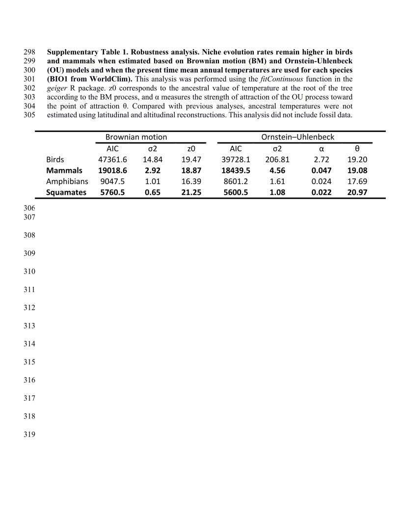
Supplementary Table 1. Robustness analysis. Niche evolution rates remain higher in birds 298 and mammals when estimated based on Brownian motion (BM) and Ornstein-Uhlenbeck 299 (OU) models and when the present time mean annual temperatures are used for each species 300 (BIO1 from WorldClim). This analysis was performed using the fitContinuous function in the 301 geiger R package. z0 corresponds to the ancestral value of temperature at the root of the tree 302 according to the BM process, and α measures the strength of attraction of the OU process toward 303 the point of attraction θ. Compared with previous analyses, ancestral temperatures were not 304 estimated using latitudinal and altitudinal reconstructions. This analysis did not include fossil data. 305

306 307

308

309

310

311

312

313

314

315

316

317

318

319

AIC σ2 z0 AIC σ2 α θBirds 47361.6 14.84 19.47 39728.1 206.81 2.72 19.20Mammals 19018.6 2.92 18.87 18439.5 4.56 0.047 19.08Amphibians 9047.5 1.01 16.39 8601.2 1.61 0.024 17.69Squamates 5760.5 0.65 21.25 5600.5 1.08 0.022 20.97

Brownian@motion Ornstein–Uhlenbeck

Supplementary Table 2. Number of fossil occurrences used to inform the most recent 320

common node of each genus in the birds phylogeny. 321

322

Birds

Nb.offossilsused

toinformthenode

Aythya 38

Anas 165 Perisoreus 3 Streptopelia 4 Gallirallus 3

Crinifer 1 Melospiza 6 Aegypius 2 Chenonetta 2

Nycticorax 8 Circus 5 Milvus 3 Pelecanoides 5

Pandion 10 Molothrus 6 Tadorna 9 Cyanoramphus 2

Haliaeetus 14 Cardinalis 4 Caprimulgus 2 Eudyptes 5

Meleagris 45 Zonotrichia 12 Oceanites 4 Coenocorypha 2

Spheniscus 18 Accipiter 25 Colius 4 Apteryx 2

Phalacrocorax 80 Melanerpes 15 Pachyptila 8 Megadyptes 3

Fulmarus 11 Passerina 1 Scopus 1 Hemiphaga 2

Sula 34 Junco 8 Leptoptilos 8 Anthornis 1

Buteo 70 Zenaida 21 Turnix 6 Thalassarche 2

Gavia 40 Colaptes 27 Passer 1 Petroica 1

Morus 29 Passerculus 4 Ploceus 2 Hymenolaimus 1

Puffinus 69 Tyto 33 Coturnix 13 Coracopsis 1

Diomedea 9 Passerella 2 Ephippiorhynchus 2 Leptopterus 1

Uria 21 Picoides 6 Hirundo 8 Foudia 1

Cepphus 6 Aphelocoma 4 Carduelis 6 Upupa 1

Oceanodroma 2 Podiceps 28 Gypaetus 1 Terpsiphone 1

Dromaius 10 Vermivora 2 Athene 11 Mirafra 1

Calonectris 6 Coragyps 16 Parus 3 Zosterops 1

Ortalis 4 Columba 24 Jabiru 4 Oreortyx 3

Tympanuchus 10 Bubo 33 Alauda 7 Loxia 3

Strix 17 Sturnella 11 Eremophila 8 Bombycilla 1

Geranoaetus 5 Coccyzus 4 Sturnus 11 Menura 1

Ardea 31 Glaucidium 4 Otis 4 Brachyramphus 2

Burhinus 5 Euphagus 6 Surnia 5 Rissa 3

Mycteria 10 Asio 20 Apus 3 Aegotheles 1

Grus 33 Dryocopus 4 Gallus 9 Collocalia 1

Aramus 5 Tachybaptus 2 Pyrrhocorax 11 Cinclosoma 2

Balearica 2 Hylocichla 2 Casuarius 1 Ptilonorhynchus 1

Anhinga 16 Ammodramus 3 Cerorhinca 6 Cacatua 2

Egretta 14 Buteogallus 3 Synthliboramphus 12 Anthochaera 2

Ardeola 1 Cyanocitta 12 Alca 25 Phaps 2

Jacana 4 Porzana 21 Aethia 4 Dasyornis 2

Phoenicopterus 10 Turdus 46 Haematopus 7 Glossopsitta 1

Fulica 27 Dumetella 2 Pluvialis 7 Platycercus 1

Bartramia 5 Chondestes 2 Bulweria 1 Phalaropus 2

Falco 62 Toxostoma 4 Fratercula 15 Neochen 1

Aquila 23 Catharus 3 Procellaria 2 Pagophila 1

Ptychoramphus 9 Spizella 6 Sterna 3

Mergus 29 Calidris 13 Pterodroma 9

Ceryle 1 Cathartes 16 Chloephaga 3

Podilymbus 31 Aegolius 8 Rhea 10

Corvus 82 Quiscalus 9 Nothura 2

Agelaius 15 Pica 10 Pygoscelis 4

Rallus 38 Recurvirostra 5 Vultur 2

Aix 8 Somateria 8 Sarcoramphus 2

Bucephala 13 Pelecanus 9 Eudromia 2

Limnodromus 6 Charadrius 12 Columbina 4

Colinus 24 Cistothorus 3 Milvago 4

Butorides 6 Caracara 17 Arenaria 4

Ciconia 19 Pipilo 4 Crypturellus 1

Gallinula 13 Icterus 2 Syrigma 1

Spizaetus 4 Anser 24 Thinocorus 3

Gymnogyps 18 Xanthocephalus 3 Theristicus 1

Gallinago 7 Tachycineta 4 Alle 18

Botaurus 8 Lophodytes 7 Dendragapus 5

Laterallus 5 Numenius 13 Cyrtonyx 3

Nyctanassa 6 Cygnus 17 Callipepla 1

Tringa 13 Melanitta 12 Pavo 1

Dendrocygna 8 Stercorarius 6 Sayornis 4

Scolopax 14 Larus 36 Petrochelidon 2

Ixobrychus 3 Aechmophorus 5 Contopus 2

Eudocimus 12 Megaceryle 3 Sitta 5

Branta 34 Dendrocopos 4 Phaethon 1

Oxyura 3 Limosa 7 Carpodacus 3

Plegadis 4 Struthio 72 Chaetura 2

Otus 21 Francolinus 28 Pinicola 2

Bonasa 12 Numida 14 Piranga 2

Genus


common node of each genus in the mammals phylogeny. 324

325

Arctonyx 9 Desmodus 16 Dasyprocta 6 Mystromys 21 Leopoldamys 3 Natalus 1

Nb.offossilsused Cuon 16 Pan 2 Marmosa 14 Malacothrix 7 Petromus 1 Mogera 3toinformthenode Rattus 34 Hydrochoerus 19 Tamandua 4 Sylvicapra 6 Gerbillurus 1 Pteromys 1

Ellobius 18 Eothenomys 2 Mormoops 5 Choloepus 3 Dendrohyrax 5 Lagostomus 28 Hylobates 1Viverra 24 Pongo 16 Antidorcas 146 Myoprocta 2 Oryctolagus 58 Myocastor 15 Pseudois 1Giraffa 252 Trachypithecus 7 Litocranius 3 Potos 3 Nesokia 7 Chaetophractus 16 Peroryctes 2Lutra 42 Macropus 94 Aepyceros 146 Caluromys 4 Thamnomys 3 Zaedyus 12 Dasyuroides 1Tapirus 246 Dasyurus 10 Damaliscus 131 Monodelphis 2 Miniopterus 21 Microcavia 10 Eligmodontia 2Potamochoerus 60 Boselaphus 1 Connochaetes 158 Metachirus 4 Grammomys 1 Lestodelphys 7 Abrothrix 1Moschus 9 Bison 263 Hippotragus 76 Ateles 3 Atelerix 3 Akodon 7 Neotomys 1Muntiacus 34 Rangifer 76 Oryx 41 Chiropotes 1 Zelotomys 8 Oxymycterus 3 Capromys 3Crocidura 145 Redunca 116 Kobus 321 Pithecia 1 Zenkerella 2 Reithrodon 13 Auliscomys 1Blarinella 10 Atlantoxerus 26 Madoqua 27 Mesomys 2 Rousettus 8 Phyllotis 7 Pecari 2

Anourosorex 8 Sciurus 104 Otocyon 12 Proechimys 8 Neotragus 2 Galea 8Myotis 231 Ochotona 117 Mellivora 44 Philander 4 Crossarchus 2 Holochilus 11Eptesicus 73 Sicista 43 Papio 83 Bradypus 3 Scutisorex 2 Ozotoceros 6Pipistrellus 31 Apodemus 313 Pedetes 11 Priodontes 2 Heliosciurus 1 Calomys 10Plecotus 34 Micromys 37 Thryonomys 43 Neacomys 1 Bdeogale 1 Lophostoma 1Callosciurus 5 Chironectes 3 Caracal 41 Rhipidomys 2 Funisciurus 2 Leptonycteris 2Tamiops 3 Aotus 3 Ichneumia 8 Mazama 22 Protoxerus 2 Chimarrogale 2Dremomys 6 Presbytis 1 Cephalophus 59 Petauroides 2 Nyctereutes 41 Murina 4Hylopetes 12 Manis 10 Phacochoerus 90 Melomys 2 Anomalurus 1 Petaurista 3Mus 61 Thylamys 7 Lycaon 17 Antechinus 10 Macroscelides 3 Chiropodomys 1Hystrix 203 Noctilio 5 Theropithecus 179 Planigale 1 Meriones 22 Burramys 2Macaca 70 Thyroptera 3 Mungos 9 Sminthopsis 8 Glis 73 Pseudochirops 2Martes 66 Leopardus 15 Loxodonta 137 Lagorchestes 2 Cricetus 94 Macroderma 2Felis 174 Lutreolina 6 Ceratotherium 205 Thylogale 4 Calomyscus 3 Dendrolagus 2Sus 182 Lepus 301 Diceros 96 Petaurus 4 Eliomys 106 Euphractus 7Rhinoceros 85 Bassariscus 45 Tragelaphus 391 Cercartetus 1 Phascogale 2 Andinomys 2Gazella 424 Perognathus 136 Tatera 46 Aepyprymnus 6 Sarcophilus 7 Euryzygomatomys 1Antilope 86 Spermophilus 388 Cercocebus 11 Bettongia 5 Phascolarctos 6 Hippocamelus 4Equus 1578 Catagonus 15 Syncerus 111 Wallabia 3 Vombatus 6 Graomys 1Hippopotamus 452 Thomomys 207 Genetta 33 Isoodon 3 Lasiorhinus 2 Balantiopteryx 1Cervus 399 Onychomys 61 Rhynchocyon 8 Perameles 8 Potorous 4 Liomys 3Capreolus 80 Antrozous 22 Civettictis 4 Pseudocheirus 5 Nyctophilus 1 Dolichotis 5Erinaceus 73 Geomys 171 Raphicerus 110 Trichosurus 12 Mastacomys 2 Blastocerus 2Hyaena 85 Ammospermophilus 20 Cercopithecus 25 Hydromys 2 Hypsiprymnodon 1 Lyncodon 1Canis 713 Lasiurus 28 Colobus 11 Uromys 1 Strigocuscus 3 Pteronotus 3Vulpes 234 Parascalops 19 Aethomys 41 Pteronura 3 Muscardinus 61 Chrotopterus 1Ursus 346 Baiomys 25 Aonyx 26 Bassaricyon 2 Desmana 61 Lonchophylla 1Panthera 329 Nasua 7 Arvicanthis 22 Callicebus 1 Episoriculus 42 Necromys 3Microtus 816 Taxidea 62 Thallomys 27 Lagothrix 1 Meles 52 Lagidium 4Capra 41 Cynomys 85 Chlorocebus 12 Saguinus 3 Talpa 210 Colomys 1Bos 158 Scapanus 49 Scotophilus 4 Saimiri 1 Lagurus 36 Kerodon 1Procavia 83 Cryptotis 41 Nycteris 4 Dactylomys 1 Urotrichus 10 Vicugna 1Hipposideros 31 Neurotrichus 3 Jaculus 5 Oecomys 2 Spalax 32 Aplodontia 5Rhinolophus 81 Tayassu 31 Mastomys 21 Oligoryzomys 4 Soriculus 7 Pappogeomys 2Tadarida 29 Cerdocyon 6 Xerus 16 Nectomys 2 Galemys 14 Solenodon 1Dasypus 83 Notiosorex 23 Taphozous 6 Marmosops 1 Neomys 20 Macrotus 3Tamias 63 Reithrodontomys 85 Helogale 10 Callithrix 1 Dryomys 8 Brachyphylla 3Didelphis 44 Cratogeomys 22 Gerbillus 30 Dinomys 1 Cricetulus 27 Nycticeius 2Sylvilagus 275 Eumops 11 Pelomys 9 Alcelaphus 126 Arvicola 92 Geogale 2Blarina 82 Histiotus 1 Acomys 10 Acinonyx 28 Hemitragus 23 Microgale 6Scalopus 55 Dipodomys 135 Heterocephalus 14 Cabassous 1 Mesocricetus 5 Tenrec 2Sorex 516 Erethizon 66 Paraxerus 11 Microsciurus 1 Chionomys 2 Pteropus 1Marmota 104 Chrysocyon 5 Lemniscomys 14 Dasymys 16 Vormela 3 Microcebus 2Castor 172 Antilocapra 29 Myosorex 12 Lophuromys 2 Axis 8 Cheirogaleus 2Oryzomys 40 Orthogeomys 7 Suncus 23 Praomys 24 Myospalax 12 Lemur 2Peromyscus 309 Phenacomys 61 Eidolon 2 Cricetomys 4 Rupicapra 4 Propithecus 2Sigmodon 201 Lasionycteris 3 Galago 12 Graphiurus 12 Hemiechinus 1 Avahi 1Neotoma 318 Microdipodops 3 Heterohyrax 8 Sylvisorex 3 Barbastella 4 Fossa 1Neofiber 37 Oreamnos 9 Heteromys 3 Hylochoerus 6 Nyctalus 3 Cryptoprocta 1Ondatra 162 Myodes 124 Eira 4 Ictonyx 7 Rhizomys 10 Nesomys 1Synaptomys 73 Chaetodipus 22 Galictis 3 Proteles 9 Allactaga 8 Echinops 1Zapus 39 Ovis 90 Molossops 2 Cryptomys 22 Dorcopsis 3 Triaenops 1Urocyon 53 Enhydra 22 Molossus 3 Cynictis 18 Viverricula 1 Mormopterus 1Tremarctos 26 Lemmus 41 Artibeus 5 Elephantulus 32 Atherurus 3 Eliurus 2Procyon 92 Lemmiscus 28 Carollia 1 Amblysomus 6 Asellia 1 Paradoxurus 1Mustela 231 Brachylagus 8 Glossophaga 2 Steatomys 20 Tarsius 3 Uropsilus 1Spilogale 63 Ochrotomys 7 Micronycteris 4 Dendromus 21 Megaderma 8 Tylonycteris 1Mephitis 48 Glaucomys 26 Phyllostomus 3 Saccostomus 32 Ctenomys 27 Trichys 1Conepatus 19 Podomys 11 Sturnira 2 Otomys 34 Scaptonyx 5 Elaphodus 1Lontra 32 Tamiasciurus 33 Trachops 2 Rhabdomys 8 Alticola 1 Budorcas 1Lynx 161 Alces 50 Rhogeessa 2 Atilax 14 Eolagurus 4 Phyllops 1Odocoileus 237 Condylura 12 Alouatta 5 Bathyergus 18 Cavia 9 Gracilinanus 2Puma 51 Napaeozapus 9 Cuniculus 8 Suricata 7 Hylomys 5 Scapteromys 2Hydropotes 5 Vespertilio 10 Rhynchonycteris 1 Georychus 3 Ratufa 4 Clyomys 1Elephas 85 Gulo 22 Tonatia 2 Parotomys 2 Tupaia 3 Thrichomys 1Crocuta 142 Myrmecophaga 5 Cebus 4 Chrysochloris 8 Nycticebus 1 Prionailurus 1Paguma 4 Dicrostonyx 27 Zygodontomys 4 Tachyoryctes 15 Belomys 2 Lutrogale 1Herpestes 62 Ovibos 37 Coendou 8 Poecilogale 1 Niviventer 7 Babyrousa 2

Genus


common node of each genus in the amphibians and squamates phylogenies. 327

328

Squamata Amphibians

Nb.offossilsused Nb.offossilsused

toinformthenode toinformthenode

Ophisaurus 107 Salamandra 20

Uromastyx 4 Pelodytes 6

Sceloporus 42 Plethodon 7

Anolis 25 Rana 212

Gerrhonotus 12 Pseudotriton 1

Rhineura 11 Bufo 195

Leiocephalus 7 Ambystoma 96

Eumeces 38 Hyla 64

Holbrookia 10 Barbourula 1

Phrynosoma 25 Tylototriton 2

Heloderma 4 Necturus 2

Crotaphytus 13 Cryptobranchus 8

Gambelia 1 Amphiuma 9

Uta 1 Siren 30

Anniella 2 Scaphiopus 28

Varanus 35 Rhinophrynus 2

Egernia 2 Taricha 3

Blanus 13 Spea 32

Chalcides 8 Andrias 13

Trogonophis 1 Acris 10

Lacerta 82 Pseudacris 21

Tarentola 3 Pseudobranchus 5

Agama 3 Notophthalmus 12

Tropidophorus 2 Gyrinophilus 3

Chamaeleo 8 Gastrophryne 6

Eremias 2 Discoglossus 12

Amphisbaena 2 Xenopus 6

Urosaurus 2 Litoria 3

Elgaria 1 Limnodynastes 3

Paroedura 1 Pelobates 30

Zonosaurus 1 Triturus 22

Furcifer 1 Alytes 2

Callisaurus 1 Bombina 5

Ameiva 3 Eupsophus 1

Sauromalus 1 Lechriodus 1

Aristelliger 1 Ceratophrys 2

Sphaerodactylus 1 Leptodactylus 3

Leiopelma 3

Eleutherodactylus 7

Desmognathus 7

Eurycea 1

Chioglossa 1

Laliostoma 1

Ptychadena 1

Scaphiophryne 1

Rhacophorus 1

Dicamptodon 1

Lissotriton 5

Mertensiella 1

Genus Genus

Documents

The impact of endothermy on the climatic niche evolution