Embed Size (px)
Citation preview
Agricultural and Resource Economics Review 40/1 (April 2011) 63–80 Copyright 2011 Northeastern Agricultural and Resource Economics Association
The Impact of Reducing Greenhouse Gas Emissions in Crop Agriculture: A Spatial- and Production-Level Analysis Lanier Nalley, Mike Popp, and Corey Fortin With the Waxman-Markey Bill passing the House and the administration’s push to reduce car-
bon emissions, the likelihood of the implementation of some form of a carbon emissions pol-icy is increasing. This study estimates the greenhouse gas (GHG) emissions of the six largest row crops produced in Arkansas using 57 different production practices predominantly used and documented by the University of Arkansas Cooperative Extension Service. From these GHG emission estimates, a baseline state “carbon footprint” was estimated and a hypothetical GHG emissions reduction of 5, 10, and 20 percent was levied on Arkansas agriculture using a cap-and-trade method. Using current production technology and traditional land use choices, results show that the trading of carbon-emitting permits to reduce statewide GHG emissions by 5 percent from the baseline would enhance GHG emissions efficiency measured as net crop farm income generated per unit of carbon emissions created. The 5 percent reduction in GHG emissions does cause marginal reductions in acres farmed and has marginal income ramifica-tions. Beyond the 5 percent reduction target, gains in GHG emissions efficiency decline but remain positive in most counties through the 10 percent GHG reduction target. However, with a 10 percent GHG reduction, acreage and income reductions more than double compared to the 5 percent level. When GHG emissions are reduced by 20 percent from the baseline, the re-sult is a major cropping pattern shift coupled with significant reductions in traditional row crop acreage, income, and GHG emissions efficiency.
Key Words: greenhouse gas emissions, carbon equivalents, sustainability, cap and trade With the Waxman-Markey Bill passing the House and the administration’s push to reduce green-house gas (GHG) emissions by late 2009, the likelihood of the implementation of some form of a carbon emissions policy is increasing. While GHG emissions have been modeled for quite some time, many policy analyses to date have focused either on global/national effects on agriculture (Reilly and Paltsev 2009, Outlaw et al. 2009, Beckman, Hertel, and Tyner 2009, McCarl 2007), individual field test plots, or soil- and climate-based models that work at the field level (Century
Model 1995, Parton et al. 1987). The former lack detail at the local level while being representative and relevant at the macro level, while the latter prove very detail-oriented, but findings can often not be generalized to larger regions and hence typically lack inclusion of likely responses to changing economic conditions. Therefore, a meth-odology to both measure GHG emissions and ana-lyze carbon emission policy impacts that strikes a middle ground is needed—a methodology suffi-ciently detailed to embody local production, soil, and climate differences, and yet sufficiently re-presentative to provide pertinent economic infor-mation for agricultural producers and policymak-ers at the local, county, state, and federal levels. The purpose of this study is to estimate and analyze GHG emissions of the six largest row crops (corn, cotton, rice, sorghum, soybeans, and wheat) produced in Arkansas across the range of the most predominant production practices docu-mented by the University of Arkansas Coopera-
_________________________________________
Lanier Nalley is Assistant Professor, Mike Popp is Professor, and CoreyFortin is Research Assistant in the Department of Agricultural Eco-nomics and Agribusiness at the University of Arkansas in Fayetteville, Arkansas.
This project was supported by a grant from Cotton Incorporated. Fur-ther support and resources were provided by the University of Arkan-sas Center for Agricultural and Rural Sustainability, the USDA Coop-erative State Research, Education, and Extension Service (CSREES), the Arkansas Agricultural Experiment Station, and the U.S. Depart-ment of Energy.

64 April 2011 Agricultural and Resource Economics Review
tive Extension Service (UACES). The estimation of GHG emissions by production method uses a cradle-to-farm gate Life Cycle Analysis (LCA) on a county-by-county basis and offers the opportu-nity of estimating the trade-offs between GHG emis-sions and agricultural returns between crops and within crops using different production methods. More specifically, GHG emissions were esti-mated by crop and production practice, varying within and across counties in conjunction with cost of production data, allowing for the estima-tion of impacts of various carbon-reduction poli-cies on (i) county and agricultural income redis-tribution throughout the state as a result of crop acreage reallocation, (ii) crop acreage realloca-tion, which in turn is affected by the capping of GHG emissions, and (iii) the capping of GHG emissions itself. The objectives of this study are to (i) quantify the amount of GHG emissions as they vary by crop, production practice, and county, (ii) calculate crop acreage reallocation and farm income redistribution at the county level when GHG emissions are reduced with a cap-and-trade system from a 2007 baseline by 5, 10, and 20 per-cent, and (iii) compare changes in carbon emis-sion efficiency measured as net crop farm income generated per ton of carbon emissions created. Background Life Cycle Analysis The Life Cycle Analysis (LCA) put forth in this study included both direct and indirect GHG emis-sions. Direct emissions are those that come from farm operations. Examples are carbon dioxide (CO2) emissions from the use of diesel by tractors and irrigation equipment and the use of gasoline by farm trucks. Indirect emissions, on the other hand, are emissions generated off-farm as a result of the manufacturing of inputs used on the farm. Examples are GHG emissions from the use of natural gas in commercial fertilizer production. Included in the LCA are GHG emissions of agri-cultural inputs involved in the production of commodities up to the farm gate (e.g., fertilizer, herbicides, pesticides, fuel, agricultural plastics, and other chemicals). Excluded are emissions gen-erated during drying, transport, or processing of a commodity that occurs after the farm gate. Also excluded from this study are embedded carbon
emissions as a result of upstream production of equipment and tools used on-farm for agricultural production. Finally, as is common with many LCAs, the analysis excludes those inputs that con-tribute less than 2 percent of total emissions. Methane Emissions from Rice Given that Arkansas is the largest producer of rice in the United States, methane (CH4) emis-sions—a direct result of flooded rice cultivation and the anaerobic decomposition of organic mat-ter in the soil—were included. Tyler (2009) ana-lyzed 12 rice production seasons from two south-ern rice-producing states (Texas and Louisiana) and found that the average methane released from rice production was 268.1 mg/m2 of methane per day, or an equivalent of 1,367 lbs of carbon per acre of paddy rice per year.1 Relative to the rest of the row crop agriculture, rice production thus releases a large amount of methane, a greenhouse gas 25 times more potent than carbon dioxide. Soil and Nitrogen Effects It was assumed that soil carbon remained con-stant, or at equilibrium, and so there was no net carbon sequestration or soil CO2 emission (Kahn et al. 2007) as a result of crop production. Soil nitrous oxide (N2O) emissions stemming from the application of nitrogen fertilizer have been identi-fied as a major contributor to GHG emissions from crop production (Bouwman 1996, Smith 1997, Yanai 2003, Del Grosso et al. 2005, Snyder et al. 2009). The International Panel on Climate Change (IPCC) (IPCC 2007) Third Assessment Re-port conversion factor of 298 units of CO2 emitted per unit of N2O applied is commonly used and based on a one percent emissions loss from nitro-gen application. This amounts to 1.27 lb of car-bon equivalent (CE) emissions per pound of ele-mental nitrogen applied.2 However, given the large variation in N2O release, which is a function 1 268.1 mg/m2 of methane per day times 4,046 m2/acre times 25 CO2/ CH4 times 12/44 C/CO2 divided by 453,592 mg/lb equals a carbon equivalent of 16.3 lbs/ac per day. The average number of days under the flood in Tyler’s (2009) study was 83.84, resulting in 1,367 (83.84 × 16.3) lbs of carbon equivalent per acre per year from methane release in rice production. 2 For each pound of N applied we get 44/28 N2O/N2 times 0.993 per-cent emitted times 298 CO2 / N2O times 12/44 C/CO2 equals 1.27 C/N applied.
Nalley, Popp, and Fortin The Impact of Reducing Greenhouse Gas Emissions in Crop Agriculture 65
of timing and method type of nitrogen as well as climatic and soil conditions, we chose to perform the analyses with and without this N2O emissions load. Carbon Emissions Calculations Given the above complexities in dealing with the estimation of GHG emissions, previously reported carbon equivalent (CE) emission factors were used to estimate the amount of emissions gener-ated as a result of input use by production prac-tice (Table 1). In essence, multiple GHGs associ-ated with global warming were converted to their carbon equivalents to obtain a “carbon foot-print”—a process stemming from a rich engi-neering literature on carbon equivalence. Values provided by the U.S. Environmental Protection Agency (EPA) (EPA 2007, 2009) were used for diesel and gasoline combustion emissions and combined with EcoInvent’s life cycle inventory database through SimaPro (2009) to calculate the upstream emissions from the production of fuel. Values provided by Lal (2004), a synthesis of nu-merous studies measuring carbon emissions from farm operations, were used for all other inputs. Since many different types of fertilizers (e.g., ammonium nitrate, liquid nitrogen, diammonium phosphate, urea, potash, phosphates, and combi-nations of the above) require different amounts of energy, production technologies, and hence CO2 emissions during fertilizer production, Lal’s (2004) CE emission values for nitrogen, phosphorus, and potassium were used to arrive at GHG emissions from combinations of fertilizers used in produc-tion by weighting by their component values (i.e., 1 lb of 18-24-15 N-P-K fertilizer would have 0.18 × 1.3 CE from N + 0.24 × 0.2 CE from P and 0.15 × 0.16 CE from K, or 0.31 CE per pound of 18-24-15 fertilizer applied without N2O emissions and 0.54 CE with N2O emissions). Crop Production Information Annual estimates of cost of production for each of the six largest crops are available from the University of Arkansas Cooperative Extension Service (UACES) (UACES 2008) and are reported for different soils, production regions, and pro-duction practices commonly used by producers (see the appendix for a description of major
changes in production methods). Using the car-bon equivalents from Table 1 and the recom-mended input usage from each of the 57 exten-sion production budgets, a per acre GHG emission level could be calculated for each production bud-get (Table 2). As shown, per acre GHG emissions are highest for rice production, with GHG emis-sion rates roughly four times higher than for corn, the next highest emitter. The principal component of this large carbon footprint is the methane re-leased during paddy rice production. Table 2 and Figure 1 also illustrate the differ-ence in GHG emissions per acre between irrigated and non-irrigated production methods (high-lighted in Figure 1 with the letter D for dryland or non-irrigated production). Pumping water for irrigation requires a significant amount of energy (typically diesel) and contributes significantly to the total GHG emissions when comparing irri-gated to non-irrigated production. Including or excluding N2O emissions affects corn and soy-beans the most/least, respectively, given the rela-tively high level and lack of nitrogen fertilizer application for the respective crops. The applica-tion of agricultural chemicals (pesticide, fungi-cide, and herbicide) affects the GHG emissions for cotton the most. Figure 1 demonstrates the signi-ficant impact of using different production prac-tices across different regions in the state. On aver-age, soybeans had the lowest GHG emissions per acre, followed by wheat, sorghum, cotton, corn, and rice, respectively. While these relative rankings are important, they fail to take into account the profitability of each crop. That is, if a carbon policy was implemented, that does not imply that there would be a large increase of dryland soybean acres (the smallest emitter) and a large decrease of rice acres (the largest emitter). In fact, in terms of profitability, rice is highest among the portfolio of crop land use choices available in the Arkansas Delta, and as such producers would be most reluctant to cur-tail its production. Another key point that a single “carbon emissions score” fails to take into ac-count is the efficiency of input use. As inputs re-main constant and yield increases, carbon per lb/ bushel of commodity decreases. While some crop production methods (center pivot irrigation, for example) have high levels of inputs (fuel), they also have a relatively high yield, and so the GHG emissions per lb/bushel of commodity is much closer to the mean of low-input and low-yielding

66 April 2011 Agricultural and Resource Economics Review
Table 1. Carbon Equivalent Emission Factors
Input Pounds of Carbon-Equivalent
per Unit of Input Used Source
Fuel (gal)
diesel 7.01 SimaPro (2009), EPA (2007, 2009)
gasoline 6.48 SimaPro (2009), EPA (2007, 2009)
Fertilizer (lb)
nitrogen 1.30 Lal (2004)
phosphorus 0.20 Lal (2004)
potassium 0.16 Lal (2004)
lime 0.06 Lal (2004)
N2O emissions 1.27 Solomon et al. (2007)
Herbicide/Harvest Aid/adjuvant (pt or lb) 6.44 Lal (2004)
Insecticide/fungicide (pt or lb) 5.44 Lal (2004)
Methane (acre of paddy rice) 1,367 Tyler (2009)
production practices of non-irrigated crops, for example. On the same note, as new seed tech-nologies are adopted that have lower input usage (e.g., hybrid rice) while maintaining yield, GHG emissions per lb/bushel of crop will decline as well. So, to imply that rice acreage will decrease because it has the largest carbon footprint is look-ing at only one side of the equation. Profitability in terms of input to output efficiency must be analyzed at a county level and by production method to estimate how crop land use choice will change under various carbon policies. Modeling County Crop Production
Profitability and Historical Acreage Limits
An Arkansas state model that tracks crop profit-ability and resource use similar to that used by Popp, Nalley, and Vickery (2010) was necessary to model producer behavior on a county-by-county basis. Tracking fuel, labor, fertilizer, chemi-cal, and irrigation water/plastic piping use as re-ported by UACES was used to not only calculate GHG emissions but also to conduct crop profit-ability analyses by comparing county yields and associated revenues to cost of production. Given the array of production methods discussed above (Table 2), crop-specific extension experts were consulted to determine which of the reported pro-duction methods were most prevalent in each of
the nine crop-reporting districts (CRD) as defined by the Arkansas Agricultural Statistics Service. That is, rice extension experts were asked to determine which of the eight possible rice pro-duction methods in Arkansas were most fre-quently used within each CRD. This effort re-sulted in CRD-specific cost of production and resource use estimates. County-level average yields from 2004 to 2007 (USDA 2008a) helped deter-mine returns above total specified expenses to land, management, and capital (NR), which in turn were used to model producer crop allocation decisions for all 75 counties in Arkansas. The model is constrained by historical land use decisions to reflect technological, socioeconomic, and capital investment barriers. Hence, historical information about harvested crop land (including all crops, fruits, vegetables, hay land, and hay yield), pasture, CRP, and irrigated acres was col-lected from USDA Census of Agriculture data for 1987 through 2007. County-specific average Con-servation Reserve Program (CRP) payments for 2007 were obtained from the USDA’s Farm Ser-vice Agency (USDA 2008). Data for annual har-vested acres for the traditional crops were avail-able electronically by county from the Arkansas Agricultural Statistics Service from 1975 to 2007 (USDA 2008a). With the possibility of emission restrictions re-quiring crop land to be idled, an alternative land

Nal
ley,
Pop
p, a
nd F
ortin
Th
e Im
pact
of R
educ
ing
Gre
enho
use
Gas
Em
issi
ons i
n C
rop
Agri
cultu
re
67
Tab
le 2
. Gre
enho
use
Gas
(Car
bon
Equ
ival
ent)
Exc
ludi
ng N
2O E
mis
sion
s in
Poun
ds p
er A
cre
for
Eac
h of
the
61 M
ajor
Pro
duct
ion
Met
hods
for
the
6 L
arge
st R
ow C
rops
, Hay
, Pas
ture
, and
CR
P in
Ark
ansa
s C
rop
(Reg
ion)
Pr
oduc
tion
Prac
tice
Car
bon
Equi
vale
nt
Emis
sion
(lbs
/ac)
Cro
p Pr
oduc
tion
Prac
tice
Car
bon
Equi
vale
nt
Emis
sion
(lbs
/ac)
C
orn
RR
furr
ow c
lay
soil
(1)a
571.
07
Sorg
hum
C
ente
r piv
ot lo
amy
soil
(37)
36
7.44
RR
furr
ow lo
amy
soil
(3)
492.
98
Furr
ow lo
amy
soil
(38)
33
2.46
BT/
RR
furr
ow lo
amy
soil
(4)
492.
98
Floo
d lo
amy
soil
(39)
32
6.71
BT
furr
ow lo
amy
soil
(5)
477.
59
Non
-irrig
ated
mix
ed so
il (4
0)
247.
43
C
onve
ntio
nal c
ente
r piv
ot lo
amy
soil
(2)
554.
63
C
onve
ntio
nal f
urro
w lo
amy
soil
(6)
477.
59
RR
floo
d (1
1)
232.
07
R
R fu
rrow
(12)
22
8.31
C
otto
n B
G/R
R c
ente
r piv
ot st
ale
seed
bed
12
row
(47)
46
9.50
Full-
se
ason
so
ybea
n R
R c
ente
r piv
ot (1
3)
221.
19
B
GII
/RR
Flex
cen
ter p
ivot
no-
till 1
2 ro
w (4
9)
458.
14
RR
boa
rder
irrig
ated
(17)
19
3.26
(N
orth
east
) R
RFl
ex fu
rrow
stal
e se
ed b
ed 1
2 ro
w (5
2)
455.
48
RR
non
-irrig
ated
(19)
10
9.04
LL fu
rrow
stal
e se
ed b
ed 1
2 ro
w (5
4)
440.
32
Con
vent
iona
l flo
od (1
4)
212.
82
R
R n
on-ir
rigat
ed st
ale
seed
bed
8 ro
w (5
6)
362.
94
Con
vent
iona
l fur
row
(15)
20
9.07
BG
/RR
furr
ow c
onve
ntio
nal t
ill 1
2 ro
w (4
4)
479.
42
Con
vent
iona
l cen
ter p
ivot
(16)
20
1.94
BG
/RR
cen
ter p
ivot
stal
e se
ed b
ed 1
2 ro
w (4
6)
469.
50
Con
vent
iona
l boa
rder
Irrig
ated
(18)
17
4.01
(C
entr
al)
WS/
RR
Flex
furr
ow st
ale
seed
bed
12
row
(48)
45
8.17
C
onve
ntio
nal n
on-ir
rigat
ed (2
0)
89.7
9
BG
II/R
RFl
ex fu
rrow
stal
e se
ed b
ed 1
2 ro
w (5
1)
455.
48
B
G/R
R fu
rrow
stal
e se
ed b
ed 1
2 ro
w (5
3)
455.
48
RR
furr
ow (2
1)
205.
60
R
R n
on-ir
rigat
ed st
ale
seed
bed
8 ro
w (5
7)
348.
42
RR
cen
ter P
ivot
(22)
20
5.48
BG
/RR
cen
ter p
ivot
stal
e co
nven
tiona
l till
8 ro
w (4
1)
513.
67
Dou
ble-
cr
oppe
d so
ybea
n R
R fl
ood
(23)
20
2.23
BG
/RR
furr
ow st
ale
seed
bed
8 ro
w (4
2)
480.
62
RR
cen
ter p
ivot
no-
till (
27)
173.
15
(Sou
thea
st)
BG
/RR
furr
ow c
onve
ntio
nal t
ill 1
2 ro
w (4
3)
479.
48
RR
boa
rder
irrig
ated
(28)
17
0.55
BG
II/R
RFl
ex c
ente
r piv
ot st
ale
seed
bed
12 ro
w (4
5)
470.
63
RR
furr
ow n
o-til
l (29
) 15
8.89
BG
II/R
RFl
ex fu
rrow
stal
e se
edbe
d 12
row
(50)
45
5.48
C
onve
ntio
nal c
ente
r piv
ot (2
5)
188.
33
R
R n
on-ir
rigat
ed st
ale
seed
bed
8 ro
w (5
5)
363.
30
Con
vent
iona
l fur
row
(24)
18
8.45
Con
vent
iona
l flo
od (2
6)
185.
08
Ric
eb C
onve
ntio
nal s
eed
clay
soil
(31)
2,
010.
47
Con
vent
iona
l boa
rder
irrig
ated
(30)
15
3.40
Con
vent
iona
l see
d si
lt lo
am so
il (3
2)
1,94
7.76
Con
vent
iona
l no-
till s
ilt lo
am so
il (3
4)
1,93
7.85
W
heat
A
fter r
ice
clay
(7)
284.
23
C
lear
field
silt
loam
soil
(33)
1,
942.
51
Afte
r ric
e sa
nd/s
ilt lo
am so
il (9
) 26
6.27
Hyb
rid si
lt lo
am so
il (3
5)
1,90
5.91
A
fter o
ther
cla
y so
il (8
) 27
2.25
Con
vent
iona
l zer
o gr
aded
no-
till w
ater
seed
ed (3
6)
1,85
9.98
A
fter o
ther
sand
/silt
loam
soil
(10)
24
2.31
Hay
C
onve
ntio
nal (
ferti
lized
to N
ASS
repo
rted
yiel
ds) (
58)
18
6.68
CR
P Es
tabl
ishm
ent c
harg
e fo
r gra
ss (6
1)
2
7.97
Low
inpu
t (lo
w fe
rtiliz
er 1
cut
with
wee
d co
ntro
l) (5
9)
14
9.03
Pa
stur
e Es
timat
ed fo
r 2 a
cres
per
cow
with
out l
ives
tock
em
issi
ons (
60)
97
.18
a B
udge
t num
ber f
or c
ross
refe
renc
e w
ith F
igur
e 1.
//
b Ric
e G
HG
em
issi
ons i
nclu
de th
e es
timat
ed 1
,367
lbs o
f car
bon
attri
bute
d to
met
hane
gas
rele
ase
per a
cre.
Nalley, Popp, and Fortin The Impact of Reducing Greenhouse Gas Emissions in Crop Agriculture 67

68 April 2011 Agricultural and Resource Economics Review
0
100
200
300
400
500
600
700
800
900
1 2 3Corn 4 5 6 7 8
Wheat 9 10 11 12 13 14 15
Soybeans FS 16 17 18
D 19
D 20 21 22 23 24 25
Soybeans DC 26 27 28 29 30 31 32
Rice 33 34 35 36 37 38
Sorghum 39
D 40 41 42 43 44
D 45 46
Cotton 47 48 49 50
D 51 52 53 54 55 56
D 57
Hay D 58
D 59
Pasture D 60
CRP D 61
Carbon Equivalent Em
issions (lb/ac)
Fertilizer N20 Emissions Fuel Herbicide/Harvest Aid/Adjuvant Insecticide Fungicide Figure 1. Decomposition of Total Greenhouse Gas Emissions by Crop and Production Types Note: The carbon equivalent for rice does not include the 1,367 lbs attributed to methane release. “D” symbolizes non-irrigated enterprises. The crop number immediately below the x-axis refers to the production budget number in Table 2.
use choice was created to ensure that this land would not go to weeds or cause excessive soil erosion. The enterprise alternative chosen in-volves establishment of grass that would be har-vested once per year in June or July to avoid po-tential weather-related problems with earlier har-vest. The land is minimally fertilized and con-trolled for weeds to maintain the stand. As such, low-quality hay harvested at an average yield of 1.91 dry ton per acre results in sufficient revenue to offset most production costs. This alternative was chosen in lieu of pine tree production, as output price uncertainty would be lower, initial cash outlays smaller, reversibility to crop land easier, and annual revenue streams from com-modity sales possible. This comes at the cost of lower carbon sequestration potential, the value of which is currently deemed an insignificant source of revenue at $0.20 per ton of carbon sequestered and higher emissions in comparison with pine (Smith, Popp, and Nalley 2010). Similar to Popp, Nalley, and Vickery (2010),
the net return of Arkansas crop, hay, and pasture land are maximized by choosing crop acres (x) on the basis of expected commodity prices (p), county-relevant yield (y), and cost of production informa-tion (c) as follows:
(1) Maximize NR = 75 14
1 1( ) ,j ij ijn ij
i jp y c x
= =
× − ×∑∑
subject to xmin ij ≤ xij ≤ xmaxij iacresmini ≤ ∑xij ≤ iacresmaxi for irrigated crops only acresmini ≤ ∑xij ≤ acresmaxi for all crops except pasture and CRP, where i denotes each of the 75 counties of pro-duction and j denotes 14 land management choices
Nalley, Popp, and Fortin The Impact of Reducing Greenhouse Gas Emissions in Crop Agriculture 69
(irrigated and non-irrigated crop production, hay, pasture, and CRP), and n denotes different pro-duction practices specific to production region and exogenous to the model. Xmin and xmax are historical county acreage minima and maxima over the harvest years 2000 through 2007 for each crop (USDA 2008a). Iacresmin and iacres-max are the 1987 to 2007 Census-based reported irrigated acres that reflect technological, socio-economic, and capital barriers to irrigation, again at the county level. Acresmin and acresmax are total harvested acres at the county level, as col-lected by the Census, and were amended by add-ing 10 percent of county CRP enrollments to the maximum harvested acre totals to reflect the po-tential for added acres from land coming out of CRP and the typical ten-year enrollment horizon of CRP acreage. Note that winter wheat was con-sidered part of harvested acres even though this crop can be considered in double-crop rotations with soybean, corn, or sorghum crops. Crop price information (pj) was based on the July futures prices as of December of the previous year and no commodity price program support (Great Pacific Trading Company 2008).3 Basis expectations were set to zero for all crops, and prices were ad-justed for hauling, drying, and commodity board check-off charges as appropriate. Direct and counter-cyclical payments were included in the price per unit of all crops (Table 3).4 Yields (yij) reflect the per acre county averages for most crops. Since the Arkansas field office of the Na-tional Agricultural Statistics Service (NASS) does not differentiate between irrigated and non-irriga-ted double-cropped soybean and sorghum acre-age, minor modifications as described by Popp, Nalley, and Vickery (2008) were made to double-crop soybean maximum and minimum acreage re-strictions and grain sorghum yield differences be-tween irrigated and non-irrigated production. Per acre cost of production estimates (cij) were devel-oped as reported above. 3Wheat prices were based on the May futures prices as of September of the previous year given the different planting and harvest times com-pared to spring planted crops. 4 All commodity prices were high enough that the loan deficiency pay-ments were not triggered. Model runs without government payments are available from the authors upon request.
Carbon Policy Analysis The above model [equation (1)] was run to de-velop a crop production baseline for Arkansas using 2007 conditions and resulted in a county-specific and statewide estimate of the amount of GHG emitted from agricultural production (Car-bonmax). The model could then be restricted us-ing the following constraint: (2) ∑Carbonij × xij ≤ Carbonmax × (1 – a), where Carbonij are the carbon emissions by county i for land use choice j, xij are acres in pro-duction as described above, and a represents the targeted fraction of state GHG emissions to be reduced. That is, the baseline model allows pro-ducers at a county level to allocate acreage to maximize profit around a set of historical produc-tion constraints without a carbon restriction. A statewide carbon footprint was calculated from this baseline, and then 5, 10, and 20 percent re-ductions were imposed as new model constraints. It is important to note that the carbon reduction is not a county-level reduction but rather a state-wide constraint. This implies that the most/least GHG efficient crops—generating the most income per lb of GHG emitted—would be least/most af-fected by mandated reductions in statewide GHG emissions. While the model does allow the actual tracking of overall GHG emissions by county, it does not track exactly how GHG emissions are reallocated,5 and therefore does not track cash flows that a county would pay/receive by the pur-chasing/selling of carbon emission permits. In essence, changes in county-level crop farm in-come represent only the changes associated with crop acreage reallocation. Noteworthy nonethe-less is the fact that since the transactions between buyer and seller are a zero sum gain, the total
5 For example, assume that county A and B both produce rice using only production method X (thus, theoretically the cost of production and emissions should be equivalent). If the average yield per acre in county B is 200 bu/acre and county A averages 175 bu/ac, because of the profit-maximizing nature of the model county B would continue to produce, whereas county A would curtail production if these were the only two options. Since each county grows more than one crop using an array of production techniques, it becomes difficult to track emis-sions trading where producers that curtail emissions would sell pollu-tion credits to those that continue to pollute. As such, the model also does not take into consideration the actual price of the permit nor transaction costs associated with permit trading; this is pertinent infor-mation that warrants further research.
70
Apr
il 20
11
Agri
cultu
ral a
nd R
esou
rce
Econ
omic
s Rev
iew
T
able
3. B
asel
ine
Cro
p A
crea
ge a
nd P
erce
ntag
e C
hang
e in
Sta
te C
rop
Acr
eage
Giv
en a
5, 1
0, a
nd 2
0 Pe
rcen
t Red
uctio
n in
Sta
tew
ide
Gre
enho
use
Gas
Em
issi
ons
B
asel
ine
Perc
enta
ge C
hang
e fr
om B
asel
ine
Acr
es a
nd In
com
e w
ith
GH
G E
mis
sion
s Red
uctio
n Po
licy
Scen
ario
s
$/
Cd
5%
10%
20
%
Cro
p A
cres
$/
Acr
e Pr
iceb
Gov
t. Py
mtc
Avg
. SD
w
/o N
2O
N2O
w
/o N
2O
N2O
w
/o N
2O
N2O
Cor
n (ir
rigat
ed)
520.
8 20
0 4.
00
0.11
79
8 27
3 3.
7 1.
1 0.
7 1.
9 (1
7.2)
(1
4.9)
Non
-irrig
ated
cot
ton
341.
3 11
9 0.
58
0.07
66
5 36
0 (1
.3)
nc
(9.8
) nc
(5
5.9)
(3
0.3)
Irrig
ated
cot
ton
667.
5 14
8 0.
58
0.07
62
9 15
8 12
.9
14.2
8.
4 13
.1
(18.
4)
5.6
Non
-irrig
ated
full-
seas
on so
ybea
ns
736.
4 17
7.
10
0.22
35
0 51
2 (1
.3)
16.4
13
.5
16.1
14
.1
36.5
Irrig
ated
full-
seas
on so
ybea
ns
1,65
8.7
25
7.10
0.
22
225
209
0.4
0.2
0.6
1.0
nc
1.2
Irrig
ated
dou
ble-
crop
soyb
eans
14
4.8
(22)
7.
10
0.22
(2
35)
275
nc
nc
nc
nc
nc
nc
Ric
e (ir
rigat
ed)
1,45
3.5
296
0.11
0.
01
299
37
(9.6
) (6
.2)
(12.
9)
(12.
5)
(12.
9)
(12.
9)
Whe
at (n
on-ir
rigat
ed)
844.
3 63
4.
60
0.32
49
1 17
7 (1
0.8)
(5
0.0)
(4
0.8)
(5
0.7)
(7
3.8)
(7
6.1)
Non
-irrig
ated
gra
in so
rghu
m
105.
8 78
3.
80
0.18
63
3 23
5 (6
.5)
0.1
(11.
0)
(0.4
) (4
8.8)
(4
6.3)
Irrig
ated
gra
in so
rghu
m
86.6
11
4 3.
80
0.18
65
7 17
2 17
.5
(0.4
) (2
.1)
1.0
nc
(25.
1)
Hay
land
1,
428.
2 40
60
.00
NA
42
6 19
4 (0
.3)
0.9
(24.
5)
(24.
2)
(23.
9)
(24.
5)
Low
-inpu
t hay
d 0
(4)
40.0
0 N
A
(49)
N
A
6,69
0 20
,201
20
,201
20
,201
24
,464
18
,390
CR
P 44
2.8
41
54.9
8 N
A
2,90
0 74
8 nc
nc
nc
nc
nc
nc
Past
ure
3,85
6.5
25
25.0
0 N
A
515
NA
nc
nc
nc
nc
(5
7.6)
(5
7.6)
Tota
l acr
es in
pro
duct
ion
7,99
8.0
(1
.7)
(3.2
) (9
.3)
(8.8
) (1
9.0)
(1
3.6)
Tota
l irr
igat
ed a
cres
4,
532.
0
0.3
0.3
(2.6
) (1
.4)
(9.7
) (5
.1)
Tota
l car
bon
emis
sion
s (to
ns)e
2,48
8.2
Tota
l net
retu
rns (
$)
986,
701
(2
.9)
(2.9
) (7
.6)
(7.0
) (2
2.9)
(1
8.2)
a In
thou
sand
s of u
nits
. $/a
cre
is a
crea
ge-w
eigh
ted
aver
age
retu
rns p
er c
rop.
$/C
is a
crea
ge-w
eigh
ted
base
line
net r
etur
ns p
er to
n of
car
bon
emis
sion
s with
out N
2O e
mis
sion
s. b C
orn,
whe
at, b
eans
, and
sor
ghum
are
pric
ed in
dol
lars
per
bus
hel,
rice
in d
olla
rs p
er h
undr
edw
eigh
t, an
d co
tton
in d
olla
rs p
er p
ound
of l
int.
Past
ure
is re
ntal
rate
s pe
r acr
e, C
RP
is a
vera
ge
paym
ent p
er a
cre
for t
he st
ate
but i
s cou
nty-
spec
ific,
and
hay
is b
ased
on
dolla
rs p
er to
n.
c Gov
ernm
ent p
aym
ents
are
the
sum
mat
ion
of d
irect
and
cou
nter
-cyc
lical
pay
men
ts p
er u
nit (
lb, b
ushe
l, cw
t, et
c.) p
er c
rop.
d S
tand
ard
devi
atio
n of
$/C
is b
ased
on
varia
tion
in y
ield
and
regi
on-s
peci
fic c
ost o
f pro
duct
ion.
Cos
t of p
rodu
ctio
n do
es n
ot v
ary
by y
ield
, onl
y by
pro
duct
ion
met
hod.
Pas
ture
and
low
-inpu
t ha
y ar
e m
odel
ed a
t con
stan
t pro
fit/y
ield
acr
oss c
ount
y gi
ven
lack
of d
ata
on p
rodu
ctio
n m
etho
d de
tail.
d T
he b
asel
ine
mod
el d
oes n
ot a
lloca
te a
crea
ge to
low
-inpu
t hay
. Thu
s, th
e nu
mbe
rs in
this
row
repr
esen
t tot
al a
cres
, not
per
cent
age
chan
ge fr
om th
e ba
selin
e.
e N2O
em
issi
ons a
dd 3
63,0
70 to
ns o
r 12.
8 pe
rcen
t abo
ve b
asel
ine
tota
l car
bon
emis
sion
s.
70 April 2011 Agricultural and Resource Economics Review
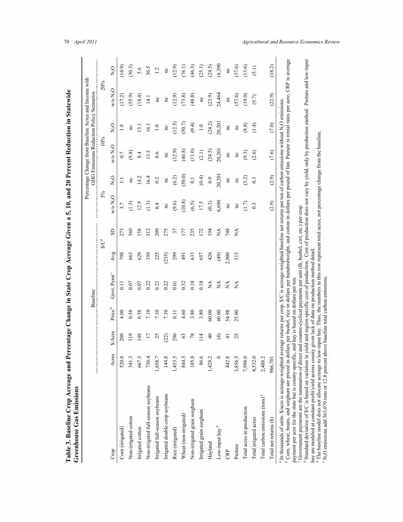
Nalley, Popp, and Fortin The Impact of Reducing Greenhouse Gas Emissions in Crop Agriculture 71
change in state crop farm income is only a func-tion of crop acreage reallocation and not affected by permit trading cash flows with the exception of transaction costs. These assumptions are non-limiting in the sense that carbon trading at current price levels, $0.20 per ton, is expected to be minimal. As shown in Table 2 and Figure 1, the largest GHG differential per acre among tradi-tional row crop land use choices is between rice and non-irrigated soybeans at 1,920.68 lbs CE/ acre. This differential in carbon emissions trans-lates to $0.19 per acre using a carbon price of $0.20/ton versus per acre net returns of $295.74 on average for rice and $17.48 on average for non-irrigated soybeans. That is, the price of car-bon would have to change substantially before a producer voluntarily switches from one acre of ir-rigated rice to one acre of non-irrigated soybeans. So, by changing the amount of GHG emissions allowed for state crop agriculture, the model can be used to determine changes in crop acreage allocation and the overall profitability implica-tions of a reduction of GHG emissions specifically targeted at Arkansas crop agriculture.6 The analy-sis does assume that producers will choose only from current production practices and does not include the possibility of the adoption of carbon-reducing production methods/technology, as cur-rent carbon prices provide little incentive to change. Excluded from the model are also moni-toring costs for enforcing carbon emission re-strictions. Another important simplifying assump-tion is no changes in input prices that are antici-pated with any sort of carbon-emission reduction policy. Since input prices are exogenous in this model, it assumes that producers will face the same input prices regardless of the emission re-duction amount. Further research is warranted on the effects of emission policies on input prices. By modeling different reductions in GHG emis-sions, estimates of crop acreage and net farm ag-ricultural income changes for each of the 75 counties in Arkansas, providing valuable insights about which crops/industries would stand to lose the most acreage or production if emission reduc-
6 This assumes that only crop agriculture in Arkansas would be in-volved and treats Arkansas like a closed economy. That is, agriculture does not trade permits with coal-powered electricity-generating facili-ties, for example. As stated previously, this also assumes that carbon sequestration is either equal to zero or not rewarded in the form of offsets.
tions were imposed on agriculture using current production technologies. This does assume that crop prices do not respond to changes in Arkan-sas crop acreage, an assumption that is put into the context of price determination by global changes in production, with Arkansas’ production playing a minor role. Results The crop-specific baseline acreage and carbon footprint from the unconstrained model are illus-trated in Table 3.7 The baseline acreage was vali-dated and found to be within 15 percent of actual 2007 planting for corn, grain sorghum, hay land, pasture, and soybeans, and within 20 percent of the actual 2007 wheat and cotton acreage. Full season soybeans and rice are estimated as the two largest crops in Arkansas, with 1.66 and 1.45 mil-lion acres, respectively. Table 3 also presents the impacts of a 5, 10, and 20 percent reduction in GHG emissions on cropping patterns, acres in production, irrigated acreage, and net agricultural returns. Figures 2 and 3 highlight differences in GHG emissions and agricultural income for vari-ous policy scenarios with and without the inclu-sion of N2O emissions. As expected with a cap-and-trade type emis-sions restriction policy, not all counties are af-fected equally, and hence some counties offer higher emission reductions than others regardless of the amount of emission restrictions imposed (Figure 2). Further, the changes in emissions re-duction by county differ whether N2O emissions are included or not. A similar observation occurs in Figure 3 when analyzing changes in income. While initial emission reductions appear to occur more in the eastern part of the state (the Arkansas Delta), where traditional row crop production oc-curs, emission reductions required to meet a statewide 20 percent goal appear to be mainly sourced from the western part of the state. As demonstrated in Table 4, this is likely a function of the amount of land use substitution possibili- 7 Interestingly, the state baseline carbon emissions with government payments (CCP and direct payments) included in the “market” price are roughly 19.3 percent (2,488.2 tons, Table 3) less than the baseline (2,968.7 tons) without the government payments. This is attributed to the fact that with government payments, dryland cotton acreage (a low emitter) increases substantially, and corn (a relatively high emitter) acreage decreases. Results without government payments are available from the authors upon request.

72
Apr
il 20
11
Agri
cultu
ral a
nd R
esou
rce
Econ
omic
s Rev
iew
With
out N
2O E
mis
sion
s 5%
10
%
20%
With
N2O
Em
issi
ons
Fi
gure
2. E
stim
ated
Per
cent
age
Cha
nges
in C
ount
y-L
evel
Agr
icul
tura
l Gre
enho
use
Gas
Em
issi
ons f
rom
a
Stat
ewid
e 5,
10,
and
20
Perc
ent (
left
to r
ight
) Cap
-and
-Tra
de G
HG
Red
uctio
n Po
licy
With
out a
nd W
ith N
2O
Em
issi
ons (
top
and
bott
om)
72 April 2011 Agricultural and Resource Economics Review

Nal
ley,
Pop
p, a
nd F
ortin
Th
e Im
pact
of R
educ
ing
Gre
enho
use
Gas
Em
issi
ons i
n C
rop
Agri
cultu
re
73
With
out N
2O E
mis
sion
s 5%
10
%
20%
W
ith N
2O E
mis
sion
s
Figu
re 3
. Est
imat
ed P
erce
ntag
e C
hang
es in
Cou
nty-
Lev
el A
gric
ultu
ral N
et In
com
e R
educ
tion
from
a S
tate
wid
e 5,
10,
and
20
Perc
ent (
left
to r
ight
) Cap
-and
-Tra
de G
HG
Red
uctio
n Po
licy
With
out a
nd W
ith N
2O E
mis
sion
s (t
op a
nd b
otto
m)
Nalley, Popp, and Fortin The Impact of Reducing Greenhouse Gas Emissions in Crop Agriculture 73
74
Apr
il 20
11
Agri
cultu
ral a
nd R
esou
rce
Econ
omic
s Rev
iew
T
able
4. C
hang
es in
Cro
p R
otat
ion
and
Car
bon-
Equ
ival
ent E
mis
sion
s for
Cou
ntie
s Sel
ecte
d on
the
Bas
is o
f Deg
ree
of L
and
Use
Sub
stitu
tion
Poss
ibili
ties a
nd O
vera
ll C
ount
y Pr
ofita
bilit
y (lo
w, h
igh,
and
med
ium
from
top
to b
otto
m) (
N2O
em
issi
ons e
xclu
ded)
C
otto
n So
rghu
m
Soyb
ean
Hay
C
ount
y M
easu
re
Cor
n Ir
r. N
on-I
rr.
Irr.
Non
-Irr
. Ir
r. N
on-I
rr.
Ric
e W
heat
C
onv.
Lo
w
Tota
l A
cres
a
NR
$/a
c --
b --
--
--
--
--
--
--
--
$4
0.30
$(
3.66
) --
$/
lb C
--
--
--
--
--
--
--
--
--
$0
.22
$(0.
02)
--
lb C
/ac
--
--
--
--
--
--
--
--
--
186.
86
149.
03
--
Min
ac
--
--
--
--
--
--
--
--
--
64,0
82
--
68,9
34
Max
ac
--
--
--
--
--
--
--
--
--
84,6
48
85,9
74
85,9
74
Bas
e ac
--
--
--
--
--
--
--
--
--
84
,648
--
84
,648
5%
c --
--
--
--
--
--
--
--
--
nc
nc
nc
10
%
--
--
--
--
--
--
--
--
--
(15,
714)
nc
(1
5,71
4)
Washington
20%
--
--
--
--
--
--
--
--
--
(1
5,71
4)
nc
(15,
714)
N
R $
/ac
$97.
79
$154
.20
$132
.39
$148
.21
$111
.00
$35.
76
$25.
22
$303
.14
$46.
69
$40.
30
$(3.
66)
--
$/lb
C
$0.4
4 $0
.33
$0.3
6 $0
.42
$0.4
5 $0
.16
$0.2
5 $0
.15
$0.1
8 $0
.22
$(0.
02)
--
lb C
/ac
503.
27
463.
10
362.
94
346.
37
247.
43
225.
55
99.4
2 1,
980.
22
255.
78
186.
86
149.
03
--
Min
ac
2,00
0 56
,700
4,
100
500
500
109,
000
20,2
00
117,
000
7,50
0 1,
495
--
190,
302
Max
ac
11,5
00
40,0
00
22,0
00
2,25
0 2,
250
143,
500
39,0
00
136,
000
42,0
00
2,21
7 37
2,88
9 36
2,84
0 B
ase
ac
11,5
00
56,7
00
22,0
00
2,25
0 2,
250
109,
000
20,2
00
119,
120
18,3
25
1,49
5 --
36
2,84
0 5%
nc
nc
nc
nc
nc
nc
10
,103
nc
(1
0,82
5)
722
nc
nc
10%
nc
nc
nc
nc
nc
nc
12
,945
(2
,120
) (1
0,82
5)
nc
nc
nc
Poinsett
20%
nc
nc
nc
nc
nc
nc
12
,945
(2
,120
) (1
0,82
5)
nc
nc
nc
NR
$/a
c $1
24.8
5 --
--
$1
08.0
6 $7
0.47
$(
16.5
9)
$(25
.35)
$2
36.2
6 $2
0.50
$4
0.30
$(
3.66
) --
$/
lb C
$0
.25
--
--
$0.3
1 $0
.28
$(0.
07)
$(0.
25)
$0.1
2 $0
.08
$0.2
2 $(
0.02
) --
lb
C/a
c 50
3.27
--
--
34
6.37
24
7.43
22
5.55
99
.42
1,98
0.22
25
5.78
18
6.86
14
9.03
--
M
in a
c 1,
600
--
--
200
200
23,0
00
13,5
00
14,0
00
1,70
0 34
,031
--
13
7,79
3 M
ax a
c 3,
500
--
--
1,50
0 1,
500
30,0
00
23,5
00
22,0
00
21,5
00
55,6
15
171,
891
169,
771
Bas
e ac
3,
481
--
--
1,50
0 1,
500
23,0
00
13,5
00
21,1
47
21,5
00
55,6
15
--
141,
243
5%
19
--
--
nc
nc
nc
nc
(7,1
47)
nc
nc
3,67
8 (3
,450
) 10
%
19
--
--
nc
nc
nc
nc
(7,1
47)
(13,
512)
nc
17
,190
(3
,450
)
White
20%
(1
,881
) --
--
nc
nc
nc
8,
188
(7,1
47)
(19,
800)
nc
17
,190
(3
,450
)
a Tot
al a
cres
exc
lude
pas
ture
, CR
P, a
nd d
oubl
e-cr
oppe
d so
ybea
ns a
s pa
stur
e ac
res
are
not c
ount
ed in
his
toric
al m
inim
um a
nd m
axim
um h
arve
sted
acr
es in
this
mod
el. D
oubl
e-cr
oppe
d so
y-be
ans a
nd C
RP
are
not i
nclu
ded
as th
ey a
re a
lway
s at m
inim
um a
crea
ge a
nd C
RP
is n
ot m
odel
ed to
hav
e su
bstit
utio
n po
ssib
ilitie
s in
the
mod
el.
b “--
” m
eans
that
the
crop
has
not
bee
n gr
own
in th
e co
unty
from
200
0 to
200
7. U
nder
tota
l acr
es th
e sa
me
sym
bol i
mpl
ies t
hat t
he m
easu
re is
not
mea
ning
ful.
c “nc
” m
eans
no
chan
ge fr
om th
e ba
se a
crea
ge o
bser
ved.
Num
bers
in p
aren
thes
es in
dica
te d
eclin
es in
acr
eage
com
pare
d to
the
base
line,
whe
reas
pos
itive
num
bers
indi
cate
inre
ased
acr
eage
.
74 April 2011 Agricultural and Resource Economics Review
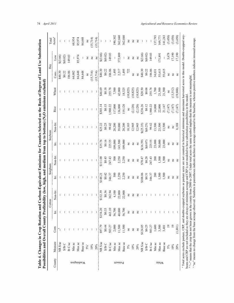
Nalley, Popp, and Fortin The Impact of Reducing Greenhouse Gas Emissions in Crop Agriculture 75
ties and the need to stay within historical acreage limits. Crop Substitution and Acreage Limits Table 4 shows detailed county-level results re-lated to Washington, Poinsett, and White coun-ties. These counties were chosen to show the im-pact of limited land use substitution possibilities as well as historical harvested acre limitations. Washington County, while profitable with hay and pasture production, has no history of row crop production, and hence the economic choice to re-duce state-level emission reductions begins to im-pact that county at the 10 percent emissions re-duction level when hay production declines. At the 20 percent emissions reduction target, pasture acres (not counted in historical harvested acres but tracked separately) go to their county mini-mum to enable a 20 percent state reduction in emissions even though these acres are still profit-able and pasture is the third lowest emitting crop (Figure 1 and Table 2). Hence, the response of Washington County with limited land use substi-tution possibilities is to curtail production only to allow more carbon-efficient counties to maintain their output level or marginally decrease their out-put to a lesser extent than Washington County. The second county analyzed in Table 4 is Poin-sett County, with the largest historical harvested acres and with the greatest number of possible choices for land use substitution. Note that in this county, production of non-irrigated soybeans—the lowest emitting crop (Figure 1 and Table 2)—and hay increases at the cost of wheat acreage to cur-tail emissions by 5 percent. Analyzing the 10 per-cent and 20 percent emissions scenario suggests a reduction of rice acreage to its historical mini-mum while adding additional non-irrigated soy-bean acres and dropping the initially added hay acres for non-irrigated soybeans with lower emis-sions. Notable, in this county is the relatively high level of profitability per acre across all enter-prises. The most carbon efficient (highest NR/lb of carbon emitted) crops stay unchanged by emis-sion restrictions, as other counties offer emission reductions at a lower overall cost to state returns and hence overall harvested acreage in the total acres column remains at historical maximum acres. White County, which has an intermediate level of land use substitution possibilities, provides
insights about how low-input hay would enter production. Also, with the exception of corn, this county exhibits less profitable yields for sorghum, soybeans, rice, and wheat than does Poinsett County, and hence acreage reductions to meet state-level emission restrictions are considered more likely. White County reallocates land use at the 5 percent emissions restriction level by first curtailing production of rice, the crop with the relatively low carbon efficiency but very high carbon emissions footprint. This allows the addi-tion of modest corn acreage to offset profitability losses but also requires the addition of low-input hay to meet the minimum total acres harvested constraint of 137,793 acres. Higher emission re-ductions come at the cost of wheat acres, the least carbon efficient of remaining crop choices for acre-age reductions (note that soybeans are already at their minima), offering a differential of approxi-mately 106 lbs of carbon/acre compared to low-input hay at a profit loss of $24.16/acre. At the 20 percent reduction level, non-irrigated soybeans, even at their greater loss to the county, offer more carbon reduction than even low-input hay, and hence enter the crop mix. Carbon Efficiency Changes Trade-offs, such as those illustrated for a sample of counties in Table 4, are also summarized in Table 5. As illustrated above, crop land use choice to minimize emissions can lead to carbon effi-ciency improvements when counties that offer lower carbon efficiency trade off emissions with counties that provide more net returns per pound of carbon emitted. Thus, while the average $/C information by crop in Table 3 is important, sig-nificant variation in profitability exists across counties primarily as a function of yield. Hence, non-irrigated cotton acreage declines at lower emission restriction levels than does irrigated cot-ton acreage, for example, even though non-irri-gated cotton acreage has a higher average carbon efficiency by shedding least efficient acres earlier than irrigated cotton acreage (note the higher stan-dard deviation in $/C for non-irrigated cotton). Further, irrigated double-cropped soybeans are already at minimum historical acreage, and hence their low carbon efficiency yields no further acre-age reduction with increasing emission restric-tions. Also note that wheat shows much higher

76 April 2011 Agricultural and Resource Economics Review
Table 5. Changes in Carbon Emissions Efficiency Across All Counties in Arkansas
Baseline
Emissions Efficiency Changes Under Policy
Scenarios a Baseline
Emissions Efficiency Changes Under Policy
Scenarios a
County C b $/C b 5% 10% 20% County C b $/C b 5% 10% 20%
Benton 28.7 476.2 0.0 0.3 (36.7) Arkansas 270.7 420.8 0.0 0.0 (13.7) Boone 22.3 491.0 0.0 1.5 (35.7) Crittenden 144.4 361.0 8.7 7.6 (9.7) Carroll 22.1 486.4 0.0 2.0 (35.0) Cross 252.0 298.4 0.0 (1.3) (11.1) Madison 22.0 479.1 0.0 2.1 (35.9) Lee 146.1 430.0 16.0 16.0 (6.8) Newton 8.0 488.9 0.0 1.9 (36.1) Lonoke 203.7 352.9 0.0 (0.0) (16.4) Washington 31.5 475.0 0.0 0.9 (36.5) Monroe 145.0 321.8 1.0 (1.7) (16.3) CRD 1 134.7 481.3 0.0 1.3 (36.1) Phillips 164.6 528.1 0.0 2.3 (19.0) Prairie 172.5 419.9 0.0 0.8 (12.9) Baxter 8.1 493.1 0.0 1.3 (36.1) Saint Francis 143.6 362.0 7.7 7.7 (10.5) Cleburne 10.5 498.9 0.0 2.9 (32.2) Woodruff 161.9 234.4 0.1 (2.5) (19.4) Fulton 19.0 499.5 0.0 1.4 (35.0) CRD 6 1,804.6 372.4 2.4 2.8 (13.5) Izard 14.8 509.7 0.0 2.2 (32.4) Marion 10.8 494.6 0.0 1.1 (35.7) Hempstead 18.6 506.5 0.0 1.2 (33.6) Searcy 13.2 492.8 0.0 1.0 (36.3) Howard 11.2 481.5 0.0 2.2 (35.3) Sharp 13.2 511.5 0.0 2.6 (32.1) Lafayette 22.7 326.8 12.4 12.4 (31.9) Stone 11.2 494.4 0.0 2.7 (33.9) Little River 16.6 518.8 0.0 0.8 (37.5) Van Buren 9.9 475.0 0.0 1.5 (36.9) Miller 36.6 319.5 6.1 6.1 (27.8) CRD 2 110.6 497.8 0.0 1.8 (34.4) Montgomery 6.7 475.7 0.0 1.6 (36.2) Pike 7.5 489.8 0.0 1.5 (35.5) Clay 210.5 392.6 0.0 0.1 (14.6) Sevier 11.6 479.3 0.0 1.7 (36.1) Craighead 244.1 426.3 0.0 0.0 (14.3) CRD 7 131.5 417.9 4.4 4.4 (33.5) Greene 170.9 336.3 0.3 0.6 (16.7) Independence 54.2 303.0 5.3 5.9 (28.5) Bradley 2.2 490.0 0.0 2.1 (33.9) Jackson 230.3 244.8 (0.8) (0.8) (14.1) Calhoun 1.5 491.3 0.0 1.5 (34.5) Lawrence 223.9 272.6 0.0 (0.9) (12.2) Clark 6.1 526.4 0.0 0.0 (32.7) Mississippi 224.1 553.3 5.1 5.7 (13.0) Cleveland 2.8 478.0 0.0 1.9 (35.4) Poinsett 311.6 361.4 0.1 0.4 (11.4) Columbia 4.1 475.9 0.0 0.6 (36.8) Randolph 95.5 385.6 4.0 7.2 (10.4) Dallas 1.5 499.3 0.0 1.6 (33.7) White 81.7 327.5 4.7 4.0 (24.4) Nevada 6.8 487.5 0.0 0.6 (35.7) CRD 3 1846.8 367.2 1.9 2.2 (13.0) Ouachita 2.4 481.3 0.0 1.2 (35.6) Union 2.7 486.2 0.0 1.6 (35.3) Crawford 15.3 512.3 0.0 2.0 (29.9) CRD 8 30.0 493.3 0.0 1.0 (34.8) Franklin 16.8 476.0 0.0 1.3 (35.7) Johnson 11.0 466.8 0.0 1.2 (37.3) Ashley 76.8 381.2 8.9 8.8 (15.8) Logan 20.7 494.7 0.0 1.4 (35.1) Chicot 120.1 464.8 1.4 2.1 (21.2) Polk 12.9 479.8 0.0 2.6 (35.2) Desha 148.3 563.4 1.9 4.1 (13.8) Pope 16.1 454.9 1.2 2.6 (35.8) Drew 53.7 359.1 12.4 12.8 (8.2) Scott 10.8 477.6 0.0 1.0 (36.4) Jefferson 171.7 370.6 1.2 3.6 (13.7) Sebastian 10.9 477.4 0.0 1.3 (35.9) Lincoln 112.5 372.5 5.2 4.5 (10.7) Yell 22.0 412.8 2.1 2.0 (33.1) CRD 9 683.0 429.6 4.0 5.5 (13.6) CRD 4 136.6 470.1 0.5 1.6 (34.7) State Total 4,976.3 389.3 2.3 2.7 (16.6) Conway 20.7 425.8 0.9 0.8 (36.8) Garland 27.2 429.6 0.8 0.6 (31.5) Grant 3.8 486.2 0.0 1.1 (37.1) Faulkner 3.3 469.4 0.0 1.9 (36.1) Hot Spring 6.1 483.0 0.0 0.9 (35.9) Perry 6.4 486.5 0.0 1.7 (34.2) Pulaski 26.4 293.2 0.6 (1.5) (29.9) Saline 4.7 484.3 0.0 1.8 (35.1) CRD 5 98.6 405.5 0.9 1.5 (33.4)
a Policy scenarios are state reductions in GHG emissions from a 2007 baseline in the amount of 5, 10, and 20 percent. b C represents carbon emisssions in thousands of pounds, and $/C tracks agricultural income per county divided by tons of carbon emitted.

Nalley, Popp, and Fortin The Impact of Reducing Greenhouse Gas Emissions in Crop Agriculture 77
acreage reductions with N2O emissions included at low levels of emission restrictions than if N2O emissions are not included. This is a direct func-tion of carbon efficiency. With N2O emissions, curtailing wheat acres allows more carbon reduc-tion benefits at relatively low profitability losses than if N2O emissions are not included, and hence state income can be maintained by shedding fewer corn acres, increasing rather than decreasing irri-gated cotton and requiring fewer low-input hay acres to meet historical harvested acreage con-straints (Table 3). Changes in Agricultural Income While minor state-level reductions in profitability at low restriction levels are evident, larger ramifi-cations become visible at the 10 percent level as even counties like Poinsett trade off profitable rice acres to meet emission restrictions. At both the 5 and 10 percent emission restriction levels, income drops by less than 5 and 10 percent be-cause of the carbon efficiency increases noted in Table 5. At the 20 percent level, however, sub-stitution possibilities that maintain total harvested acres are no longer possible and, as a last resort, crop production declines, with more or less equal declines in profitability, pending exclusion of N2O emissions. Possible Commodity Price Effects Arkansas is the largest rice producer in the United States, so a large shift away from rice production should endogenously affect domestic and to some extent world price more so than with any of the other crops considered. Under the 20 percent re-duction scenario, rice acreage declines by ap-proximately 12.9 percent. To determine whether this acreage reduction scenario would yield a sig-nificant increase in rice price, an analysis using the Arkansas Global Rice Model (Wailes and Chavez 2010) was performed and indicated that there would be a domestic price increase of ap-proximately 1.1 percent and a world price in-crease of 0.9 percent. Given that Arkansas has the largest impact in the rice market (compared to other row crops), this price change was consid-ered to be sufficiently insignificant, and other commodity price changes through emission pol-icy changes were not analyzed.
Conclusions The objective of this study was to estimate the GHG emissions, in the form of their carbon equiva-lent, as a result of production of the major crops in Arkansas. Using a cradle-to-farm gate Life Cy-cle Analysis, both direct and indirect carbon emis-sions were estimated including production prac-tice details commonly aggregated in other studies. Results of this analysis illustrate the differences in emissions on a spatial basis, as well as by production (tillage, irrigation, etc.) practice. This analysis provides a baseline for comparisons across counties and across production practices to see how inputs and spatially specific production prac-tices impact GHG emissions in production of row crops. While the results are specific to Arkansas agriculture, the methodology implemented could be applied to any region. Modeling crop production without GHG emis-sion restrictions provided a baseline of 2007 pro-duction conditions and was subsequently used to compare the introduction of cap-and-trade type GHG emission reduction policies at varying levels of intensity. Statewide restriction on GHG emis-sions led to findings that suggest that moderate reductions in emissions can lead to carbon emis-sion efficiency (dollars of output per ton of car-bon emitted) improvements as a result of emis-sions trading. Targeted emission reductions be-yond 10 percent, however, curtail carbon effi-ciency gains from trading emission permits, lower acreage in production, and significantly reduce agricultural income. Further, as a result of changes in crop mix and acreage reductions, significant spatial reallocation of producer income results in the absence of expected minor commodity price changes and no further CRP or like program acre-age payments for idled land. Ancillary effects of crop acreage changes for input and processing industries associated with agriculture in Arkansas were beyond the scope of this study but warrant further research. Also not included were transaction costs associated with enforcing emission restrictions as well as price-based incentives for pursuing less carbon inten-sive production. The analysis did show, however, that crop acre-age reallocation is sensitive to initial carbon emis-sion assumptions. That is, changing modeling as-sumptions associated with N2O emissions had an impact on crop acreage choices at the higher
78 April 2011 Agricultural and Resource Economics Review
emission reduction targets as well as for wheat—the crop most affected by N2O emissions relative to other land use choices. This suggests that, given the potential for large acreage reductions, it is quite plausible that lesser carbon emitting crops could enter the portfolio of producer land use choices, and in the event of high emission reduc-tion targets that pasture land would be diverted to alternative enterprises with potential introductions of carbon offset markets and/or energy crop mar-kets. Notable examples are CRP or like program acres as well as perennial, no-till forage and en-ergy crops like switchgrass as well as tree crops. Of considerable debate, at that point, would also be changes in carbon sequestration as a natural result of crop, tree, or dedicated energy crop pro-duction if the assumption of steady-state carbon levels in soils, as made in this analysis, were to be relaxed. In summary, modest reductions in emission tar-gets will have minor negative farm income rami-fications unless commodity prices rise to offset this effect via global declines in commodity pro-duction (all countries impose like emission re-strictions on agriculture). Also, as expected, car-bon emission efficiency increases due to gains from “trading” emission permits at modest emis-sion reduction targets. However, at high emission reduction targets, both farm income and emission efficiency are lower than the baseline. Inclusion of secondary losses in input and processing in-dustries as well as transaction costs associated with enforcing emission restrictions are expected to add to the negative aspect of mandatory emis-sion reduction policies.
References Beckman, J., T.W. Hertel, and W.E. Tyner. 2009. “Why Pre-
vious Estimates of the Cost of Climate Mitigation Are Likely Too Low”. GTAP Working Paper No. 54, Global Trade Analysis Project (GTAP), Center for Global Trade Analy-sis, Department of Agricultural Economics, Purdue Univer-sity, West Lafayette, IN. Available at https://www.gtap. agecon.purdue.edu/resources/download/4564.pdf (accessed October 22, 2009).
Bouwman, A.F. 1996. “Direct Emission of Nitrous Oxide from Agricultural Soils.” Nutrient Cycling in Agroecosys-tems 46(1): 53–70.
Century Model. 1995. “Model 4.0” Colorado State University. Available at http://www.nrel.colostate.edu/projects/century5/ (accessed October 22, 2009).
Del Grosso, S.J., W.J. Parton, A.R. Mosier, and D.S. Ojima. 2005. “DAYCENT National-Scale Simulations of Nitrous Oxide Emissions from Cropped Soils in the United States.” Journal of Environmental Quality 35(4) 1451–1460.
Great Pacific Trading Company (GPTC). 2008. “Charts and Quotes.” Available at http://www.gptc.com/quotes.html (ac-cessed June 5, 2008).
International Panel on Climate Change (IPCC). 2007. “Cli-mate Change 2007: The Physical Science Basis Contribu-tion of Working Group I to the Fourth Assessment Report of the Intergovernmental Panel on Climate Change” (edited by S. Solomon, D. Qin, M. Manning, Z. Chen, M. Marquis, K.B. Averyt, M. Tignor, and H.L. Miller). IPCC, Geneva, Switzerland.
Khan, S., R. Mulvaney, T. Ellsworth, and C. Boast. 2007. “The Myth of Nitrogen Fertilization for Soil Carbon Se-questration.” Journal of Environmental Quality 36(6): 1821–1832.
Lal, R. 2004. “Carbon Emission from Farm Operations.” Envi-ronment International 30(7): 981–990.
McCarl, B.A. 2007. “Biofuels and Legislation Linking Biofuel Supply and Demand Using the FASOMGHG Model.” Pa-per presented at the Nicolas Institute Conference: Eco-nomic Modeling of Federal Climate Proposals: Advancing Model Transparency and Technology Policy Development (July, Duke University, Durham, NC).
Outlaw, J.L., J.W. Richardson, H.L. Bryant, J.M. Raulston, G.M. Knapeck, B.K. Herbst, L.A. Ribera, and D.P. Ander-son. 2009. “Economic Implications of the EPA Analysis of the CAP and Trade Provisions of H.R. 2454 for U.S. Rep-resentative Farms.” Agricultural and Food Policy Center Research Paper No. 09-2, Texas A&M University, College Station, TX.
Parton, W.J., D.S. Schimel, C.V. Cole, and D.S. Ojima. 1987. “Analysis of Factors Controlling Soil Organic Matter Lev-els in Great Plains Grasslands.” Soil Science of America Journal 51(5): 1173–1179.
Popp, M., L. Nalley, and G. Vickery. 2008. “Expected Changes in Farm Landscape with the Introduction of a Bio-mass Market.” Proceedings paper of the Farm Foundation conference “Transition to Bioeconomy: Environmental and Rural Development Impacts” (October 15–16, St. Louis, MO). Available at http://www.farmfoundation.org/news/ articlefiles/401-Final_version_Farm_Foundation%20feb% 2020%2009.pdf (accessed October 22, 2009).
____. 2010. “Irrigation Restriction and Biomass Market Inter-actions: The Case of the Alluvial Aquifer”. Journal of Agri-cultural and Applied Economics 42(1): 69–86.
Reilly, J., and S. Paltsev. 2009. “The Outlook for Energy Al-ternatives.” Invited paper from the conference “Transition to Bioeconomy: Global Trade and Policy Issues” (March 30–31, Washington, D.C.). Available at http://www.farm foundation.org/news/articlefiles/1698-John%20Reilly%20 Paper%203-27-09.pdf (accessed October 22, 2009).
SimaPro. 2009. SimaPro 7.1, Life Cycle Assessment Software, Pré Consultants, Amersfoort, the Netherlands.

Nalley, Popp, and Fortin The Impact of Reducing Greenhouse Gas Emissions in Crop Agriculture 79
Smith, K.A., I.P. McTaggart, and H. Tsuruta. 1997. “Emis-sions of N2O and NO Associated with Nitrogen Fertiliza-tion in Intensive Agriculture, and the Potential for Mitiga-tion.” Soil Use and Management 13(4): 296–304.
Smith, A., M. Popp, and L. Nalley. 2010. “Carbon Offset Pay-ments and Spatial Biomass Supply in Arkansas: Implica-tions of Pine and Switchgrass.” Presented at the Third Na-tional Forum on Socioeconomic Research in Coastal Sys-tems, “Challenges for National Resource Economics and Policy,” New Orleans, LA (May). Available at http://www. cnrep.lsu.edu/2010/Presentations/ASmith.pdf (accessed Janu-ary 30, 2011).
Snyder, C.S., T.W. Bruulsema, T.L. Jensen, and P.E. Fixen. 2009. “Review of Greenhouse Gas Emissions from Crop Production Systems and Fertilizer Management Effects.” Agriculture, Ecosystems & Environment 133(3/4): 247–266.
Tyler, S. 2009. Personal correspondence sharing experimental data from numerous studies. Stanley Tyler, Atmospheric Sci-ence and Biogeochemistry, University of California, Irvine, CA.
University of Arkansas Cooperative Extension Service (UACES). 2008. “2007 Crop Production Budgets for Farm Planning.” Available at http://www.uaex.edu/depts/ag_ economics/previous_ budgets.htm (accessed February 23, 2010).
U.S. Department of Agriculture. 2008. “Arkansas County Data-Crops.” Arkansas field office of USDA’s National Agri-cultural Statistics Service, Little Rock, AR. Available at http://www.nass.usda.gov/QuickStats/Create_County_Indv.jsp (accessed June 7, 2008).
U.S. Environmental Protection Agency (EPA). 2007. “Inven-tory of U.S. Greenhouse Gas Emissions and Sinks: 1990–2005.” EPA Report No. 430-R-07-002, EPA, Washington, D.C.
____. 2009. “Inventory of U.S. Greenhouse Gas Emissions and Sinks: 1990–2007.” EPA Report No. 430-R-09-004, EPA, Washington, D.C.
Wailes, E.J., and E. Chavez. 2010. “Updated Arkansas Global Rice Model.” Staff Paper No. 01-2010, Department of Ag-ricultural Economics and Agribusiness, University of Ar-kansas, AR.
Yanai, J., T. Sawamoto, T. Oe, K. Kusa, K. Yamakawa, K. Sakamoto, T. Naganawa, K. Inubushi, R. Hatano, and T. Kosaki. 2003. “Spatial Variability of Nitrous Oxide Emis-sions and Their Soil-Related Determining Factors in an Ag-ricultural Field.” Journal of Environmental Quality 32(6): 1965–1977.
Appendix. Differences Within and Across Crop Enterprises
KEY FOR ABBREVIATIONS USED IN APPENDIX
ac-in acre inch RR Roundup Ready7
N nitrogen LL Liberty Link7
P phosphorus WS Roundup Ready Flex7
K potassium BG Bollgard
B boron Bt Bacillus thuringiensis
S sulfur
Corn
All corn production is irrigated using an average of 12 ac-in per production season. Fertilizer rec-ommendations are 220 lbs of N, 75 lbs of P, and 75 lbs of K—with 60 lbs of extra N on clay. All rates are elemental. Other cost differences are a function of fuel efficiency and capital cost of irri-gation method ranging from flood, furrow, to center pivot, as well as seed technology employed (conventional seed type, RR, Bt, and Bt/RR). Corn is grown mainly on loamy soils but also clay. Cotton
Cotton production occurs under both irrigated and non-irrigated conditions. Fertilizer recommenda-tions are 100 lbs of N, 60 lbs of P, 120 lbs of K, 10 lbs of B, and 1 lb of S—with 20 lbs less N for non-irrigated production. Cost differences are a function of equipment size (8 row vs. 12 row), seed technology (RR, LL, conventional seed type, WS, BG, Bt), boll weevil eradication zone, and irrigation amounts (center pivot 7 ac-in and fur-row-irrigated at 12 ac-in). Rice
All rice production is irrigated using 24–36 ac-in per production season, with zero-grade no-till fields requiring the fewest irrigation resources. All acres are flood-irrigated. Fertilizer recommen-dations range from 125 to 185 lbs of N, 0 or 60 lbs of P, and 0 or 90 lbs of K—with no P or K ap-plied on no-till and clay soils, and extra N on clay. Other cost differences are a result of plant-ing method (conventional seed type, no till, and stale seedbed) and related fuel and operating costs. Hybrid and LL varieties show significantly differ-
80 April 2011 Agricultural and Resource Economics Review
ent seed and herbicide cost. Rice is grown mainly on silt loam soil but also clay. Soybeans
Soybean production varies across irrigation method (no irrigation, center pivot, border, furrow, and flood) and seed technology (RR and conventional seed type). Fertilization recommendations include 35 lbs of P and 70 lbs of K for full season irri-gated and dryland beans, and 30 lbs of P and 35 lbs of K for double-crop irrigated soybeans. A no-till option is available for double-crop irri-gated soybeans. Wheat
Wheat production varies across soil type (clay and sand/silt loam) and planting rotation (follow-ing rice or other crops). No irrigation is assumed for all wheat as all is grown over winter. Ferti-lizer application ranges from 140 to 175 lbs of N and 70 lbs of P depending on soil type and crop rotation. Grain Sorghum
Grain sorghum production varies across irrigation type (center pivot, furrow, flood, or non-irri-gated). Fertilizer application rates are 135 lbs of N, 60 lbs of P, and 70 lbs of K—with a decrease to 110 lbs of N, 50 lbs of P, and 60 lbs of K for non-irrigated production. Other cost differences are related to irrigation fuel efficiency and capital cost. Grain sorghum is grown on loamy soils ex-clusively.
Hay
Fertilizer recommendations are 2 tons of lime at planting and 77 lbs of N, 60 lbs of P, and 60 lbs of K. All hay land is non-irrigated. Stand life is eight years, with establishment charges prorated over the useful life of the stand. Fertilizer rates are a function of average nutrient requirements for mixed hay to achieve state hay yields. Round bales are staged at the side of the field. Pasture
Fertilizer recommendation rates are 45 lbs of N, P, and K. All pasture is non-irrigated. Fertilizer recommendations are determined to ensure suffi-cient mixed forage growth to support 1 cow unit (includes calf, replacement heifer, and herd sire feeding requirements) using 2.7 acres for grazing at an estimated forage yield of 1.2 dry tons per acre. Establishment charges are similar to those for hay fields and prorated over an 8-year useful life. Lime application rates are 40 percent of those for hay. Idle Land Converted to Low Fertilizer Single Cut Hay
Fertilizer recommendations are 2 tons of lime at planting, 52 lbs of N, 45 lbs of P, and 45 lbs of K, and based on a yield target of 1.9 dry tons per acre. A single cutting is performed in June or July, and supplemental chemical weed control is assumed. Cost of establishment is prorated over an 8-year stand life.