The Impact of Skewness and Fat Tails on the Asset

March/April 2011 www.cfapubs.org 23

Financial Analysts JournalVolume 67 Number 2

©2011 CFA Institute

The Impact of Skewness and Fat Tails on the Asset Allocation Decision

James X. Xiong, CFA, and Thomas M. Idzorek, CFA

The authors modeled the non-normal returns of multiple asset classes by using a multivariatetruncated Lévy flight distribution and incorporating non-normal returns into the mean-conditionalvalue at risk (M-CVaR) optimization framework. In a series of controlled optimizations, they foundthat both skewness and kurtosis affect the M-CVaR optimization and lead to substantially differentallocations than do the traditional mean–variance optimizations. They also found that the M-CVaRoptimization would have been beneficial during the 2008 financial crisis.

lthough numerous alternatives to themean–variance optimization (MVO)framework have appeared in the litera-ture, no clear leader has emerged. The lack

of an agreed-upon alternative to MVO has slowedthe development of practitioner-oriented tools.Moreover, the difficulty in estimating the requiredinputs—returns, standard deviations, andcorrelations—for MVO is well known, a problemthat can be substantially more difficult with moreadvanced techniques. The future is hard to predictaccurately, especially in detail.

Asset class return distributions are not nor-mally distributed, but the typical Markowitz MVOframework that has dominated the asset allocationprocess for more than 50 years relies on only thefirst two moments of the return distribution.Equally important, considerable evidence showsthat investor preferences go beyond mean and vari-ance to higher moments: skewness and kurtosis.Investors are particularly concerned about signifi-cant losses—that is, downside risk, which is a func-tion of skewness and kurtosis.

Recent research suggests that higher momentsare important considerations in asset allocation.Patton (2004) showed that knowledge of bothskewness and asymmetric dependence (higher cor-relations in downside markets) leads to economi-cally significant gains, in particular, with noshorting constraints. Harvey, Liechty, Liechty, andMüller (2010) proposed a method for optimalportfolio selection involving a Bayesian decision

theoretical framework that addresses both highermoments and estimation error. They suggestedthat incorporating higher-order return distributionmoments in portfolio selection is important.

The financial crisis of 2008 has led many inves-tors to search for tools that minimize downsiderisk. In our study, we explored one of the promisingalternatives to MVO that incorporates non-normalreturn distributions: mean-conditional value at risk(M-CVaR) optimization.

Modeling Non-Normal ReturnsEmpirically, almost all asset classes and portfolioshave returns that are not normally distributed.Many assets’ return distributions are asymmetri-cal. In other words, the distribution is skewed tothe left (or occasionally the right) of the mean(expected) value. In addition, most asset returndistributions are more leptokurtic, or fatter tailed,than are normal distributions. The normal distri-bution assigns what most people would character-ize as meaninglessly small probabilities to extremeevents that empirically seem to occur approxi-mately 10 times more often than the normal distri-bution predicts.

Many statistical models have been put forth toaccount for fat tails. Well-known examples are theLévy stable hypothesis (Mandelbrot 1963), the Stu-dent’s t-distribution (Blattberg and Gonedes 1974),and the mixture-of-Gaussian-distributions hypoth-esis (Clark 1973). The last two models possess finitevariance and fat tails, but they are unstable, whichimplies that their shapes change at different timehorizons and that distributions at different timehorizons do not obey scaling relations.1

James X. Xiong, CFA, is a senior research consultant andThomas M. Idzorek, CFA, is chief investment officer anddirector of research at Ibbotson Associates, a Morningstarcompany, Chicago.

A

24 www.cfapubs.org ©2011 CFA Institute

Financial Analysts Journal

Our preferred method is based on an enhance-ment to the Lévy stable distribution model (Lévy1925). In 1963, Mandelbrot modeled cotton priceswith a Lévy stable process, an approach that waslater supported by Fama (1965). A Lévy stable dis-tribution model can have skewness and fat tails andobeys scaling properties. Unfortunately, the Lévystable distribution has infinite variance, which vio-lates empirical observations and logic that dictatesfinite return variance. Infinite variance significantlycomplicates the task of risk estimation and limits thepractical application of the stable distribution.

A simple enhancement that addresses thisshortcoming of the Lévy stable distribution is totruncate the extreme tails of the stable distribution,which results in the truncated Lévy flight (TLF)distribution (see Mantegna and Stanley 2000). TheTLF distribution is particularly well suited to finan-cial modeling because it has four finite momentsthat empirically fit the data exceptionally well; per-haps most important for financial modelers seekingan elegant modeling solution, it “scales” appropri-ately over time. More specifically, it approximatelyobeys Lévy stable scaling relations at small timeintervals and slowly converges to a Gaussian dis-tribution at very large time intervals, both of whichare consistent with empirical observations.

Xiong (2010) demonstrated that the TLF modelprovides an excellent fit for a variety of assetclasses, including the mean, asymmetries (skew-ness), and the thickness of the tails (kurtosis), aswell as the minimum and maximum returns deter-mined through the truncation process. Because wecan parametrically control skewness and kurtosis(in addition to mean and variance) with a multivar-iate version of the TLF model, it is ideal for not onlysimulating asset class returns but also studying theimpact of incorporating skewness and fat tails intothe asset allocation decision through controlledoptimizations. Thus, in our controlled optimiza-tions, in which we systematically varied the skew-ness and kurtosis of the asset classes, we used amultivariate TLF model as the basis for generatingasset returns and ultimately estimating a portfo-lio’s conditional value at risk (CVaR).

Conditional Value at RiskThe precursor to CVaR—and a slightly better-known measure of downside risk—is the standardvalue at risk (VaR), which estimates the loss that isexpected to be exceeded with a given level of proba-bility over a specified period. CVaR is closely relatedto VaR and is calculated by taking a probability-weighted average of the possible losses conditional

on the loss being equal to or exceeding the specifiedVaR. Other terms for CVaR include mean shortfall,tail VaR, and expected tail loss. CVaR is a compre-hensive measure of the entire part of the tail that isbeing observed and for many is the preferred mea-surement of downside risk. In contrast with CVaR,VaR is a statement about only one particular pointon the distribution. Studies have shown that CVaRhas more attractive properties than VaR (see, e.g.,Rockafellar and Uryasev 2000; Pflug 2000).

Artzner, Delbaen, Eber, and Heath (1999) dem-onstrated that one of the desirable characteristics ofa “coherent measure of risk” is subadditivity—thatis, the risk of a combination of investments is at mostas large as the sum of the individual risks. VaR isnot always subadditive, which means that the VaRof a portfolio with two instruments may be greaterthan the sum of the individual VaRs of those twoinstruments. In contrast, CVaR is subadditive.

In the most basic case, if one assumes thatreturns are normally distributed, both VaR andCVaR can be estimated by using only the first twomoments of the return distribution (see, e.g.,Rockafellar and Uryasev 2000).

(1)

and

(2)

where P and P are the mean and the standarddeviation of the portfolio, respectively. For ourstudy, we fixed the probability level for the VaR andthe CVaR at 5 percent (corresponding to a confi-dence level of 95 percent). For example, for a port-folio with P = 10 percent and P = 20 percent, theVaR and the CVaR of the portfolio are VaRP = 23.0percent and CVaRP = –31.2 percent of the portfolio’sstarting value. To investors, this –31.2 percent is theaverage tail loss when a loss exceeds a threshold—in our example, the worst 5th percentile of thereturn distribution.

Introducing skewness (or asymmetry) andkurtosis into a portfolio’s return distribution com-plicates the calculation of CVaR and brings us toEquation 3:

(3)

where f (c,s,k) is a function of confidence level c,skewness s, and kurtosis k.2 Unfortunately, thefunction f (c,s,k) is complicated and generally has noclosed-form solution. With Monte Carlo simula-tions based on the TLF distribution, however, wecan model non-normal returns and ultimately esti-mate Equation 3.

VaRP P P= −μ σ1 65. ,

CVaRP P P= −μ σ2 06. ,

CVaRP P Pf c s k= − ( )μ σ, , ,



M-CVaR OptimizationTraditional MVO leads to an efficient frontier thatmaximizes return per unit of variance or, equiva-lently, minimizes variance for a given level of return.In contrast, M-CVaR maximizes return for a givenlevel of CVaR or, equivalently, minimizes CVaR fora given level of return.

The M-CVaR process that we used in our studytakes non-normal return characteristics into con-sideration and, in general, prefers assets with pos-itive skewness, small kurtosis, and low variance. Ifthe returns of the asset classes are normally distrib-uted or if the method used to estimate the CVaRconsiders only the first two moments, both MVOand M-CVaR optimization lead to the same effi-cient frontier and, thus, the same asset allocations.To understand the implications of skewness andkurtosis for portfolio selection, one must estimateCVaR in a manner that captures the important non-normal characteristics of the assets in the opportu-nity set and how those non-normal characteristicsinteract when combined into portfolios.

Armed with a measure of CVaR that accountsfor skewness and kurtosis, we studied the impact ofskewness and kurtosis on asset allocation in a seriesof five comparisons. We started with a simple hypo-

thetical example and eventually moved on to a moreapplicable 14-asset-class example. More specifi-cally, Scenarios 1–4 involved four simple hypothet-ical examples, whereas Scenario 5 consisted of areal-world opportunity set of 14 asset classes.

In Scenario 1, in which we assumed normalreturns, we used a traditional quadratic optimiza-tion routine to determine the optimal portfolios. InScenarios 2–4, which involved non-normal returndistributions, we used simulation-based optimiza-tions for both MVO and M-CVaR.3 We simulatedasset returns by using multivariate TLF distribu-tion models. Such models result in return distribu-tions that incorporate variance, skewness, andkurtosis into the CVaR estimate. Appendix A pro-vides additional details on the simulation.

Hypothetical Asset ClassesTo isolate the impact of skewness and kurtosis on M-CVaR optimization, we ran a controlled experimentwith a small asset universe so that we could easilysee the insights. We assumed four simple hypothet-ical assets—Assets A, B, C, and D. The expectedreturns, standard deviations, and correlation matrixare shown in Table 1 (Panels A and B). Panel C ofTable 1 identifies the skewness and kurtosis for the

Table 1. Capital Market Assumptions with Higher MomentsExpected Return Standard Deviation

A. Expected returns and standard deviations

Asset A 5% 10%Asset B 10 20Asset C 15 30Asset D 13 30

Asset A Asset B Asset C Asset DB. Correlation matrix

Asset A 1.00Asset B 0.34 1.00Asset C 0.32 0.82 1.00Asset D 0.32 0.82 0.71 1.00

C. Skewness and kurtosis

Scenario 1Skewness 0 0 0 0Kurtosis 3 3 3 3

Scenario 2Skewness 0 0 0 0Kurtosis 3.5 3.5 6 3.5

Scenario 3Skewness 0 0 –0.5 –0.3Kurtosis 6 6 6 6

Scenario 4Skewness 0 0 –0.5 –0.3Kurtosis 3.5 3.5 6 3.5



four assets used in the first four scenarios. The nor-mal distribution has zero skewness and a kurtosis of3. A kurtosis greater than 3 indicates a fatter tail thanthat of the normal distribution. The multivariateTLF model can take the inputs shown in Table 1 andgenerate the corresponding multivariate returnsthat we used for the first four scenario analyses.

Assets A, B, and C have the same ratio of returnto risk (standard deviation), 0.5. Asset D has aslightly lower return-to-risk ratio, 0.43. The correla-tion between Asset A and the other assets is “low,”whereas the correlations among Assets B, C, and Dare “high.” One can think of Asset A as a bond indexand Assets B, C, and D as equity indices.

We analyzed the asset allocations as we variedthe skewness and kurtosis of the four assets. As canbe seen in Panel C of Table 1, by varying the skew-ness and kurtosis of Asset C relative to the otherassets, we were able to use Asset C as our primaryguinea pig. We selected a skewness of –0.5 and akurtosis of 6 (Panel C) in such a way that they aretypical values for equity asset classes.4 Because MVOignores higher moments, the optimal allocations arenearly the same for the four scenarios based onMVO.5 In contrast, one would expect the M-CVaRoptimizations to lead to different allocations.

Scenario 1. Zero Skewness and Uniform TailsZero skewness means symmetrical distributions,and uniform tails means that the kurtosis for allassets in a universe is the same. In our simplestscenario, the returns of all four hypothetical assetsare assumed to be multivariate and normally dis-tributed, with a kurtosis of 3. Table 2 shows eightoptimal allocations, ranging from low return (lowrisk) to high return (high risk). For both MVO andM-CVaR, the only constraint is no shorting. In ourstudy, we used expected return as the basis of MVO

versus M-CVaR optimization comparisons, givenour two definitions of risk. Note that the optimalallocations for the MVO and the M-CVaR optimi-zation are the same. Returning to Equation 2, wecan see that this intuitive result flows directly fromthe fact that minimizing CVaR (when estimatedunder Equation 2) is equivalent to minimizingeither P or for a given P.

If all four assets have symmetrical return dis-tributions but uniformly fat tails with a kurtosisgreater than 3, the MVO and the M-CVaR optimi-zation lead to very similar allocations, as reportedin Table 2. The reason is that when the kurtoses forall the assets are uniformly higher, their individualcontributions to the overall portfolio’s CVaR willbe higher in absolute value, but not on a relativebasis. In other words, the relative (percentage) con-tribution to the portfolio’s CVaR for each assetremains the same. The equivalency of the assetallocations provides empirical evidence that fattails alone do not invalidate MVO.6

Scenario 2. Zero Skewness and Mixed TailsIn Scenario 2, the skewness for all four assets isassumed to be approximately zero and the amountof kurtosis associated with each asset varies.7 AssetsA, B, and D have relatively thin tails with a kurtosisof 3.5, and Asset C has a fat tail with a kurtosis of 6.In the absence of skewness, Scenario 2 tests whethervarious levels of kurtosis affect asset allocations.

Table 3 shows the results. As one might expect,at an equivalent expected return, the M-CVaR opti-mizations have significantly lower allocations toAsset C—the only fat-tailed asset in this scenario—than do the MVO allocations. The M-CVaR optimi-zation lowers the portfolio’s CVaR by decreasingallocations to Asset C.

σP2

Table 2. Scenario 1: Zero Skewness and Normal Tails

Exp. Ret. = 7% Exp. Ret. = 9% Exp. Ret. = 11% Exp. Ret. = 13%

MVO M-CVaR MVO M-CVaR MVO M-CVaR MVO M-CVaR

Asset A 70.9% 70.9% 54.5% 54.5% 37.3% 37.3% 16.4% 16.4%Asset B 18.3 18.3 8.4 8.4 0.0 0.0 0.0 0.0

Asset C 10.9 10.9 30.6 30.6 49.3 49.3 65.7 65.7

Asset D 0.0 0.0 6.5 6.5 13.4 13.4 17.9 17.9

Total 100.0% 100.0% 100.0% 100.0% 100.0% 100.0% 100.0% 100.0%

Std. dev. 11.2% 11.2% 14.9% 14.9% 19.4% 19.4% 24.4% 24.4%

Skewness 0.0 0.0 0.0 0.0 0.0 0.0 0.0 0.0

Kurtosis 3.0 3.0 3.0 3.0 3.0 3.0 3.0 3.0

VaR –11.5% –11.5% –15.6% –15.6% –21.1% –21.1% –27.3% –27.3%

CVaR –16.1% –16.1% –21.7% –21.7% –29.0% –29.0% –37.3% –37.3%



Scenario 2 also highlights one of the weak-nesses of VaR. For an expected return of 13 percent,the CVaR is 0.9 percentage point less extreme forthe M-CVaR optimization than for the MVO. Incontrast, for the same two portfolios, the VaR is 1.6percentage points more extreme for the M-CVaRthan for the MVO. We can observe similar behav-iors for all four expected returns shown in Table 3,which is equivalent to saying that attempts to lowerthe VaR inadvertently increase the CVaR. Thisunwanted result is rooted in the fact that VaR is nota coherent measure of risk.

Scenario 3. Non-Zero Skewness and Uniformly Fat TailsIn Scenario 3, Assets A and B have zero skewnessand Assets C and D have (bad) skewness of –0.5 and–0.3, respectively. All four assets are assumed tohave a kurtosis of 6. Scenario 3 tests the impact ofvarious levels of skewness when tails are uniform.

The optimization results are displayed inTable 4. In the M-CVaR optimization, the alloca-tions to Asset C range from 3.9 to 9.4 percentagepoints lower than the corresponding MVO alloca-tions. This outcome suggests that when kurtosis iscontrolled, the M-CVaR optimization tends toavoid the negatively skewed assets in order to min-imize the CVaR. The more negative the skewness,the higher the tail loss, or CVaR. In other words,when all assets in the universe have uniformly fattails, the net impact is from skewness.

Scenario 4. Non-Zero Skewness and Mixed TailsThe skewness in Scenario 4 is the same as in Sce-nario 3 (Assets A and B with 0 and Assets C and Dwith –0.5 and –0.3, respectively); however, the kur-tosis of the assets varies. Assets A, B, and D all have

a kurtosis of 3.5, whereas Asset C has a disadvan-tageous kurtosis of 6. Scenario 4 tests the impact ofvarious levels of skewness and kurtosis on assetallocations.

As expected, Table 5 reports that in the M-CVaR optimization, the allocations to Asset C rangefrom 5.6 to 20.7 percentage points lower than thosein the MVO, an additional reduction of 2.6–3 per-centage points compared with Scenario 2, in whichall the assets have zero skewness. Among the fourscenarios, Asset C has the lowest allocations. For anexpected return of 13 percent, the portfolio’s stan-dard deviation is 0.5 percentage point higher for theM-CVaR optimization but its CVaR, or expected tailloss, is reduced by 1.3 percentage points.

Summarizing Scenarios 1–4Figure 1 summarizes the impact of skewness andkurtosis on the asset allocation differences thatresult from MVO and M-CVaR optimization asmeasured by the allocation to Asset C, our guineapig asset. Across all four scenarios, MVO led tosimilar asset allocations at each of the correspond-ing expected return points. Again, the observeddifferences are due to sampling errors—that is,slight differences in the return vector, standarddeviation vector, and correlation matrix for Scenar-ios 2–4. In contrast, the M-CVaR optimizationincorporated skewness and kurtosis into the assetallocation decision, which led to different optimalmixes—the allocations to Asset C varied by 20 per-centage points when changes were made to skew-ness and kurtosis. Scenario 2 suggests that kurtosiswith mixed tails has a significant impact eventhough the asset return distributions are symmet-rical. Scenario 3 implies that skewness has a signif-icant impact when kurtosis is controlled. Scenario4 shows that the combination of skewness andkurtosis with mixed tails has the largest impact.

Table 3. Scenario 2: Zero Skewness and Mixed Tails



Asset A 71.0% 68.2% 52.8% 47.3% 35.8% 25.7% 16.9% 4.5%Asset B 18.8 24.6 13.9 23.2 5.1 23.4 0.6 22.4

Asset C 10.1 7.1 28.8 20.6 46.6 33.2 63.5 45.9

Asset D 0.0 0.1 4.5 8.9 12.5 17.8 18.9 27.2

Total 100.0% 100.0% 100.0% 100.0% 100.0% 100.0% 100.0% 100.0%

Std. dev. 11.2% 11.3% 14.8% 14.9% 19.3% 19.6% 24.2% 24.6%

Skewness 0.0 0.0 0.0 0.0 0.0 0.0 0.0 0.0

Kurtosis 3.34 3.26 4.0 3.6 4.6 3.9 4.9 4.0

VaR –11.36% –11.43% –14.9% –15.3% –19.9% –20.8% –25.4% –27.0%

CVaR –16.63% –16.57% –23.4% –23.0% –32.4% –31.8% –42.2% –41.3%



Table 4. Scenario 3: Non-Zero Skewness and Uniformly Fat Tails Exp. Ret. = 7% Exp. Ret. = 9% Exp. Ret. = 11% Exp. Ret. = 13%


Asset A 72.1% 68.8% 56.0% 52.5% 37.7% 33.6% 17.2% 13.1%Asset B 16.2 22.6 6.1 11.9 0.5 6.9 0.0 5.1

Asset C 11.4 7.5 31.0 25.5 48.7 41.3 65.2 55.8

Asset D 0.3 1.2 6.9 10.1 13.1 18.2 17.7 26.0

Total 100.0% 100.0% 100.0% 100.0% 100.0% 100.0% 100.0% 100.0%

Std. dev. 11.3% 11.3% 14.9% 15.0% 19.5% 19.5% 24.4% 24.6%

Skewness –0.1 –0.1 –0.3 –0.3 –0.4 –0.3 –0.4 –0.3

Kurtosis 4.2 4.1 4.7 4.5 5.2 4.9 5.4 5.1

VaR –12.1% –12.3% –16.4% –16.6% –22.2% –22.5% –28.8% –29.3%

CVaR –19.1% –19.0% –26.9% –26.7% –37.2% –37.0% –48.2% –47.9%

Table 5. Scenario 4: Non-Zero Skewness and Mixed TailsExp. Ret. = 7% Exp. Ret. = 9% Exp. Ret. = 11% Exp. Ret. = 13%


Asset A 71.3% 66.0% 53.4% 44.2% 35.8% 22.9% 16.7% 2.9%Asset B 18.1 28.6 11.9 28.9 4.4 27.8 0.1 23.8

Asset C 10.6 5.0 29.1 17.3 46.6 29.4 63.1 42.4

Asset D 0.0 0.4 5.6 9.6 13.3 20.0 20.1 30.9

Total 100.0% 100.0% 100.0% 100.0% 100.0% 100.0% 100.0% 100.0%

Std. dev. 11.3% 11.3% 14.8% 15.1% 19.3% 19.8% 24.3% 24.8%

Skewness –0.1 –0.1 –0.3 –0.2 –0.4 –0.3 –0.4 –0.3

Kurtosis 3.3 3.2 4.0 3.5 4.6 3.7 4.8 3.9

VaR –11.9% –12.0% –16.2% –16.7% –22.2% –23.1% –28.7% –29.9%

CVaR –17.6% –17.4% –25.7% –25.1% –36.0% –34.9% –46.8% –45.5%

Figure 1. Allocations to Asset C in the Efficient Frontier with Portfolio Return of 11 Percent for the Four Scenarios

MVO M-CVaR

Percent

60

50

40

30

20

10

0Scenario 1 Scenario 4Scenario 3Scenario 2



These four scenarios provide useful insights.In an asset universe with mixed tails, informationabout skewness and kurtosis can significantlyaffect the optimal allocations in the M-CVaR opti-mization. In these cases, the CVaR, or expected tailloss, can be reduced by performing the M-CVaRoptimization but not the MVO. The reduced CVaRfor the two optimizations depends on the distribu-tions of skewness and kurtosis in the asset universeshown in Panel C of Table 1. In the M-CVaR opti-mization, wider ranges of skewness and kurtosisamong the assets lead to a greater reduction in theportfolio’s CVaR.

Scenario 5. The 14 Asset ClassesIn our final example, Scenario 5, we move awayfrom our four asset classes and apply MVO and M-CVaR to a robust 14-asset-class opportunity set thatis typical for a sophisticated investor. The 14 assetclasses and various historical descriptive statisticsare shown in Table 6.8 We measured the historicalmean, standard deviation, skewness, kurtosis,Sharpe ratio, CVaR, and “CVaR ratio” from Febru-ary 1990 to May 2010. The CVaR ratio measuresrisk-adjusted performance in the same way as theSharpe ratio, except that the denominator is CVaR.In Table 6, we can see that emerging markets havethe largest tail loss, U.S. bonds have the best Sharpeand CVaR ratios, and non-U.S. developed equitieshave the worst Sharpe and CVaR ratios.

In contrast to our previous four scenarios—inwhich we used the multivariate TLF distribution(parameterized on the basis of the capital marketassumptions in Table 1) to estimate CVaR—in Sce-nario 5, we switched to a nonparametric bootstrap-ping analysis based on historical data. This

approach allows other researchers to duplicate thisportion of our analysis because few practitionershave a workable version of the multivariate TLFdistribution.9

Rather than simply use pure historical returns,we used the reverse optimization procedure basedon the capital asset pricing model—the startingpoint for the Black–Litterman model—to infer theexpected future return for each asset class (shownin the second column of Table 7).10 We used thecapitalization-based weights (as of May 2010) in thefirst column to back out the expected returns for the14 asset classes. We then “shifted” the location ofthe historical return distribution by either addingor subtracting a constant (the difference betweenthe reverse-optimized return and the historicalaverage return) to or from each historical return. Byadding or subtracting an asset-class-specific con-stant to or from each historical return series, wefound that the standard deviation, skewness, kur-tosis, and correlation matrix of the adjusted returnsremain the same as those of the historical returns.

The expected Sharpe ratios and the expectedCVaR ratios in Table 7 are quite different from theircorresponding historical ratios in Table 6 owing tothe substantial differences between expectedreturns and historical returns. The emerging mar-kets asset class continues to have the largestexpected tail loss. Non-U.S. developed equities hasthe largest expected Sharpe and CVaR ratios. U.S.bonds has the lowest expected Sharpe ratio,whereas U.S. Treasury Inflation-Protected Securi-ties (TIPS) has the lowest expected CVaR ratio.

Next, we performed bootstrapping analysesby randomly drawing from these “shifted” histor-ical return distributions. Conceptually, the starting

Table 6. Historical Descriptive Statistics for the 14 Asset Classes, February 1990–May 2010Mean Std. Dev. Skewness Kurtosis Sharpe Ratio CVaR CVaR Ratio

Large value 10.24% 14.70% –0.82 5.06 0.44 –36.37% 0.18Large growth 9.34 17.40 –0.64 4.19 0.32 –41.46 0.13

Small value 12.62 17.07 –0.86 5.16 0.51 –42.84 0.20

Small growth 9.47 23.23 –0.41 3.84 0.24 –51.71 0.11

Non-U.S. dev. equities 5.85 17.45 –0.52 4.29 0.11 –40.90 0.05

Emerging markets 13.29 24.26 –0.74 4.72 0.39 –56.11 0.17

Commodities 7.13 15.58 –0.57 6.67 0.21 –35.00 0.09

Non-U.S. REITs 8.05 20.66 –0.22 5.03 0.20 –46.44 0.09

U.S. REITs 15.31 20.36 –0.76 10.51 0.56 –49.50 0.23

U.S. TIPS 8.19 5.54 –0.89 8.27 0.78 –11.74 0.37

U.S. bonds 7.22 3.82 –0.31 3.72 0.89 –6.77 0.50

Non-U.S. bonds 7.67 8.76 0.17 3.54 0.44 –15.89 0.24

Global high yield 10.89 10.59 –1.60 12.50 0.67 –27.13 0.26

Cash 3.85 1.98 –0.26 2.26 0 0.03 0



shifted historical return distribution can be thoughtof as the best guess for the unknown “population”distribution in which each random draw results inone possible sample distribution that could be thebest representation of the unknown true futuredistribution. The bootstrapping, or resampling,method simultaneously accounts for input uncer-tainty and addresses the issues of estimation error,input sensitivity, and highly concentrated assetallocations.

Because CVaR is a tail measure, each drawnsample needed to contain adequate tail informa-tion, and thus, the number of data points in eachdraw could not be too small. We simply set thenumber of draws equal to the available historicaldata period: February 1990–May 2010, or 244months. Therefore, the left tail contained about 12data points (= 5 percent 244) each time a newsample distribution was created. We repeated theM-CVaR optimization and the MVO 500 differenttimes for 500 different sample distributions. All theresults were recorded and averaged to derive theaverage optimal asset allocations over the 500 pos-sible realized futures.

To ensure diversification, we limited the max-imum allocation for each asset class to 30 percentduring each optimization. To mitigate the issue of“optionality” associated with long-only con-straints in resampling (see Scherer 2002), weallowed short sales and limited shorting to 30 per-cent for each asset class. Optionality means thatassets are either in or out but are never negative inlong-only resampled asset allocations, and thus,higher-volatility assets tend to receive higher allo-cations (on average) relative to long–short resam-pled asset allocations.

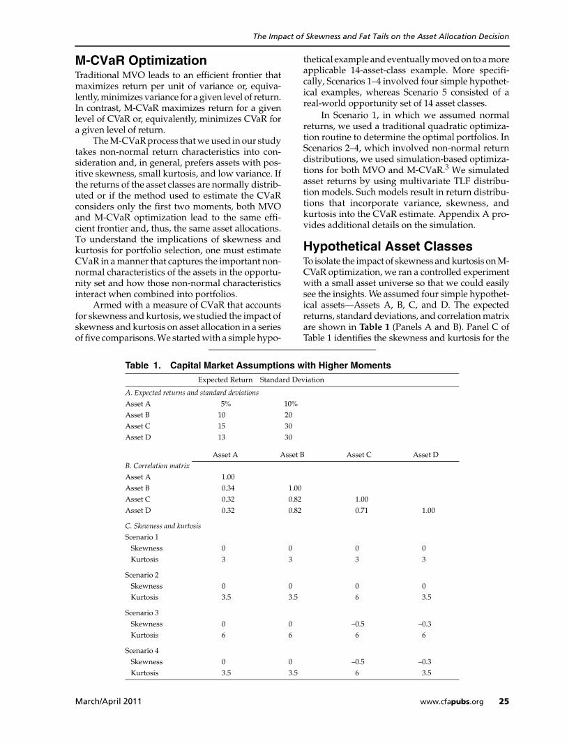
Figure 2 shows the skewness and kurtosis forthe 14 asset classes over the last 20 years (1990–2010). Note that the relationship between skewnessand kurtosis is somewhat linear for all 14 assetclasses. A higher kurtosis is often accompanied bymore extreme negative skewness. Also note thatglobal high yield, U.S. REITs, and U.S. TIPS appearin the bottom right of Figure 2, which suggests thatthey have high kurtosis and more extreme negativeskewness. From this perspective, these three assetshave characteristics that are similar to those of AssetC in Scenario 4. Empirically, these assets seem toproduce relatively stable returns during normaltimes, but they can suffer severely negative returnsduring extraordinary events. For U.S. REITs, thisoutcome is perhaps due to larger-than-normalamounts of leverage coupled with unusuallysmooth returns because of the large dividend com-ponent of returns. For U.S. TIPS and global highyield, we performed an “exceedence correlation”analysis to estimate asymmetrical correlations andfound that their correlation with the U.S. equitymarket is asymmetrically much higher in severedownside markets than in normal markets or upmarkets.11 This finding is directly related to nega-tive skewness and higher kurtosis.

Table 8 shows the optimal asset allocations forboth the MVO and the M-CVaR optimization fromthe bootstrapping of the 14 asset classes. As before,we identified efficient asset allocations from theMVO and M-CVaR optimization approaches basedon expected returns. We selected four asset mixes(AM1–AM4), with expected returns of 7 percent, 9percent, 11 percent, and 13 percent for each boot-strapping, respectively. Many of the different assetallocations between the M-CVaR and the MVO aresignificant at the 5 percent level. For example, the

Table 7. Expected Descriptive Statistics for the 14 Asset Classes Capitalization

WeightsExpected

MeanSharpeRatio

ExpectedCVaR

CVaRRatio

Large value 8.70% 8.94% 0.36 –36.62% 0.14Large growth 8.67 9.54 0.34 –41.29 0.14

Small value 0.83 9.12 0.32 –43.66 0.12

Small growth 0.76 10.71 0.31 –51.23 0.14

Non-U.S. dev. equities 16.01 10.53 0.40 –39.50 0.18

Emerging markets 4.82 11.88 0.35 –56.30 0.15

Commodities 5.80 6.33 0.16 –35.16 0.07

Non-U.S. REITs 7.98 11.31 0.38 –45.41 0.17

U.S. REITs 3.51 9.24 0.27 –50.97 0.11

U.S. TIPS 0.84 4.78 0.15 –12.64 0.06

U.S. bonds 23.12 4.49 0.13 –7.49 0.07

Non-U.S. bonds 16.04 5.51 0.18 –16.44 0.10

Global high yield 1.92 7.10 0.31 –28.07 0.12

Cash 0.98 4.00 0 0.10 0



M-CVaR optimization allocates significantlyhigher amounts, by about 4.5 percentage points, tonon-U.S. government bonds and significantlylower amounts, by about 3 percentage points, toglobal high yield for all the expected return levels.

These two asset classes are the polar points alongthe skewness axis in Figure 2.

Compared with the MVO, the M-CVaR opti-mization monotonically underweights global highyield, U.S. REITs, and commodities because of their

Figure 2. Skewness and Kurtosis for the 14 Asset Classes, February 1990–May 2010

Table 8. Bootstrapped Optimal Allocations and Statistics for the 14 Asset ClassesAM1 AM2 AM3 AM4



Large value 1.13% 0.59% 3.52%* 2.15%* 5.79%* 3.80%* 8.88%* 6.87%*Large growth 3.29* 4.63* 3.79 4.52 4.93 5.70 7.67 8.04Small value 7.54* 8.51* 5.48 6.03 4.52 4.77 5.28 5.79Small growth –2.35* –1.37* –1.36* –0.04* 0.08* 1.74* 1.91* 4.01*Non-U.S. dev. equities 2.82* –0.45* 5.25* 2.47* 8.54* 7.08* 12.05 11.36Emerging markets 1.31 1.53 1.56 1.18 2.94 2.35 5.48 4.94Commodities 3.62* 1.12* 4.03* 1.38* 4.71* 2.17* 4.85* 2.59*Non-U.S. REITs –2.83 –2.55 0.01* 2.33* 3.49* 6.19* 7.75* 10.70*U.S. REITs –2.55* –4.36* –0.74* –3.42* 1.75* –1.69* 4.73* 0.98*U.S. TIPS 15.55 15.17 13.46* 15.51* 11.89* 14.42* 8.10* 10.33*U.S. bonds 28.18 28.30 22.91* 24.11* 17.35* 20.26* 11.16* 14.46*Non-U.S. bonds 9.27* 15.62* 9.01* 14.10* 8.82* 12.27* 8.08* 11.02*Global high yield 5.01* 3.29* 5.22* 2.26* 5.01* 1.53* 4.86* 0.72*Cash 30.00 29.97 27.84 27.40 20.19* 19.40* 9.19* 8.19*

Total 100.0% 100.0% 100.0% 100.0% 100.0% 100.0% 100.0% 100.0%

Std. dev. 4.0% 4.6% 6.0% 6.7% 8.5% 9.2% 10.8% 11.5%Skewness –0.4 0.3 –0.3 0.3 –0.3 0.1 –0.4 0.0Kurtosis 5.0 3.7 4.9 3.9 5.0 4.2 5.1 4.3

VaR –4.8% –4.7% –7.6% –7.5% –11.4% –11.1% –14.8% –14.7%CVaR –7.3% –6.0% –11.4% –9.8% –16.9% –15.1% –22.1% –20.4%

*Significant at the 5 percent level.

Skewness

Non-U.S. Bonds

CashSmall Growth

Non-U.S. Dev.Large Growth

EmergingLarge Value

Small Value

Commodities

U.S. TIPSU.S. REITs

Non-U.S. REITsU.S. Bonds

Global High Yield

0.5

0

–0.5

–1.0

–1.5

–2.00 4 8 12

Kurtosis



more extreme negative skewness and higher kur-tosis, and it overweights non-U.S. governmentbonds, U.S. nominal bonds, and non-U.S. REITsbecause of their more attractive combined skew-ness and kurtosis. Small growth receives higherweights in the M-CVaR optimization owing to itsattractive upper-left position in Figure 2 (higherskewness and lower kurtosis), even though theweights are negative (short sales) for AM1 andAM2. Non-U.S. developed equities closely matchessmall growth in all four moments, as shown inTable 6, but it is located below and to the right ofsmall growth and thus receives less weight in theM-CVaR than in the MVO.

Note that the M-CVaR, compared with theMVO, allocates 4.8 percentage points less weight toU.S. TIPS in the asset mix with an expected returnof 5 percent (not shown in Table 8) but allocates 2.2percentage points more weight to U.S. TIPS in AM4,with an expected return of 13 percent. The alloca-tions to TIPS are reduced as the expected return isincreased for both the M-CVaR and the MVO, butthe reduced amount is less for the M-CVaR (5.9percentage points) than for the MVO (13.0 percent-age points) when the expected return is increasedfrom 5 percent to 13 percent. The main reason is thatthe M-CVaR is relatively less sensitive to expectedreturn than is the MVO, and the CVaR measure putsmore weight on skewness and kurtosis.

A portfolio’s skewness or kurtosis is not sim-ply the linear combination of individual assetclasses’ skewness or kurtosis. Because the M-CVaRminimizes a portfolio’s CVaR, or tail loss, an indi-vidual asset class’s higher-moment informationshould not be considered entirely separately. Thispoint reinforces the most important lesson of mod-ern portfolio theory: Although individual assetclass characteristics are important, what really mat-ters is the portfolio’s overall characteristics.

In general, these observations are consistentwith our previous discussions of Scenarios 2–4: TheM-CVaR optimization tends to pick positivelyskewed (or less negatively skewed) and thin-tailedassets, whereas the MVO ignores the informationfrom skewness and kurtosis. At the portfolio level,the skewness is higher, the kurtosis is lower, andthe CVaR is lower for the M-CVaR optimization.For example, as shown in the bottom of Table 8 forAM4, the expected volatility is increased by 0.7percentage point, but the skewness is increasedfrom –0.4 to 0, the kurtosis is lowered by 0.8, andthe CVaR is lowered by 1.7 percentage points.

Note that bootstrapping allows us to obtainsome estimates on sampling error for the CVaR. Asmentioned earlier, CVaR is a tail-loss measure thatcan suffer from estimation errors. For example, for

AM4 in Table 8, the mean of the estimated CVaRsover the 500 samples is –20.4 percent (last row, lastcolumn), but the variations of those CVaRs are 18percent in terms of standard deviation. That is, thebulk of the CVaRs range from –2.4 percent to –38.4percent, which is quite wide. In terms of standarddeviation, the average variations of optimal alloca-tions for each asset are about 25 percent over the500 sample multivariate distributions. For AM1,the corresponding CVaRs range from –4.0 percentto –8.0 percent, which is much narrower than therange for AM4. The average variations of optimalallocations for each asset are about 12 percent forAM1. A larger sample can reduce CVaR estimationerror, but the trade-off is that a larger sample is lessefficient for resampling. More specifically, a largersample increases the likelihood that the sampleparameters will converge to the starting inputs(population parameters), which will increase thesimilarity of the optimal asset allocations from dif-ferent bootstrapped samples.

M-CVaR vs. MVO in the Financial Crisis of 2008To test whether the M-CVaR optimization, com-pared with the MVO, would have helped investorsduring the financial crisis of 2008, we ran an out-of-sample bootstrapping analysis.12 The bootstrap-ping procedure is the same as the one describedearlier except that it was performed in August 2008,right before the onset of the most dramatic part ofthe financial crisis. The historical skewness and kur-tosis from February 1990 to August 2008 are shownin the second and third columns of Table 9. Notethat absent the data from September 2008 on, thevalues for skewness are higher and the values forkurtosis are lower for most equity classes, REITs,and commodities. In other words, the 2008 crisissignificantly shifted their left tails further to the left.In particular, commodities were positively skewedbefore the crisis but were significantly negative afterthe crisis. In sharp contrast, the crisis made theskewness of U.S. bonds less negative, which sug-gests that the crisis triggered the flight to safety.

As before, we selected four asset mixes (AM1–AM4) for each resampled portfolio, with expectedreturns of 7 percent, 9 percent, 11 percent, and 13percent, respectively. We set the minimum andmaximum allocations for each asset class at –30percent and 30 percent, respectively. We repeatedthe M-CVaR optimization and the MVO 500 timesand recorded the average optimal asset allocations.The differences in average allocations between theM-CVaR and the MVO for the four asset mixes areshown in Table 9 (from column 5 to the last column).



A negative sign means that the asset class has alower weighting based on the M-CVaR optimiza-tion. Overall, the allocation differences shown inTable 9 are similar to those shown in Table 8, exceptfor U.S. bonds and commodities. The oppositechanges in skewness for U.S. bonds and commodi-ties owing to the crisis resulted in higher allocationsto commodities and lower allocations to U.S. bondsfor the M-CVaR optimization in Table 9 comparedwith that in Table 8.

The duration of our out-of-sample testingperiod was six months (September 2008–Febru-ary 2009). No rebalancing occurred during thesesix months. For the 14 asset classes, the losses orgains during the six months are shown in thefourth column of Table 9: U.S. REITs suffered thehighest loss (–58.39 percent), followed by com-modities (–48.47 percent). The outperformance ofthe M-CVaR optimization over the MVO is shownin the last row of Table 9. Note that the M-CVaRoutperformed the MVO in all four asset allocationmixes, with excess returns ranging from 0.84 per-centage point to 1.44 percentage points.

Across the four asset mixes, on average, the M-CVaR optimization overweights non-U.S. bondsover global high yield, as well as non-U.S. REITsover U.S. REITs. It also underweights non-U.S.developed equities and emerging markets. Twoadverse allocations made by the M-CVaR optimi-zation are the overweighting in commodities andthe underweighting in U.S. bonds relative to the

MVO because the asset class commodities (U.S.bonds) has favorable (unfavorable) pre-crisis skew-ness. The majority of these allocation differences,however, turn out to be effective, which leads to theoverall outperformance for the M-CVaR. This out-performance suggests that the higher-momentinformation embedded in historical returns hadsome predictive power in the crisis.13

ConclusionAlthough practitioners are well aware that assetreturns are not normally distributed and thatinvestor preferences often go beyond mean andvariance, the implications for portfolio choice arenot well known.

In a series of controlled traditional MVOs andM-CVaR optimizations, we gained insights into theramifications of skewness and kurtosis for optimalasset allocations. In our first four scenarios, prior torunning the optimizations, we used the multivari-ate TLF distribution model to simulate a large num-ber of returns with appropriate variance, skewness,and kurtosis, which, in turn, enabled us to moreaccurately measure the downside risk of a portfolioby using the CVaR.

In our first example, in which returns are sym-metrically distributed and have uniform tails, theMVO and the M-CVaR lead to the same results.When there are varying levels of skewness andkurtosis in the opportunity set of assets, the MVOand the M-CVaR lead to significantly different asset

Table 9. Out-of-Sample Test for M-CVaR and MVO in the Financial Crisis of 2008

Skewnessa KurtosisaGain/Loss in

Crisis AM1b AM2b AM3b AM4b

Large value –0.53 4.48 –39.98% 0.68 –0.32 –1.06 –1.19Large growth –0.52 4.17 –34.54 1.63 1.64 1.06 0.02

Small value –0.74 4.56 –42.47 0.08 1.30 1.41 0.73

Small growth –0.32 3.91 –41.91 –0.33 0.09 0.97 1.91

Non-U.S. dev. equities –0.29 3.44 –41.26 –2.44 –1.83 –0.52 0.46

Emerging markets –0.70 4.45 –39.62 –0.63 –1.99 –2.87 –2.40

Commodities 0.13 3.58 –48.47 –0.17 0.08 0.64 0.99

Non-U.S. REITs 0.01 4.50 –46.27 1.14 2.53 3.25 2.93

U.S. REITs –0.30 3.81 –58.39 –0.90 –2.52 –2.91 –2.88

U.S. TIPS –0.33 4.67 –2.06 1.53 4.14 3.77 3.48

U.S. bonds –0.38 3.67 3.29 –1.71 –0.96 –0.13 –0.19

Non-U.S. bonds 0.18 3.56 0.87 3.95 2.44 1.92 1.79

Global high yield –1.22 10.36 –20.76 –2.72 –3.68 –4.46 –4.53

Cash –0.20 2.45 0.44 –0.12 –0.91 –1.06 –1.12

M-CVaR return less MVO return 1.11 1.44 1.15 0.84aSkewness and kurtosis were measured from February 1990 to August 2008.bColumns AM1–AM4 show the optimal allocation differences, measured in percentage points, between M-CVaR and MVO for eachasset class for the four asset mixes.



allocations. In particular, the combination of a neg-ative skewness and a fat tail has the greatest impacton the optimal asset allocation weights. Intuitively,the M-CVaR prefers assets with higher positiveskewness, lower kurtosis, and lower variance.

Over the last 20 years, global high yield, U.S.REITs, U.S. TIPS, and value stocks had significantnegative skewness, whereas non-U.S. governmentbonds had positive skewness. The kurtosis forglobal high yield, U.S. REITs, and U.S. TIPS washigher than it was for other asset classes. In a 14-asset-class bootstrapping analysis, the M-CVaR,relative to the MVO, led to significantly higherallocations to non-U.S. government bonds and U.S.nominal bonds and lower allocations to global highyield, U.S. REITs, and commodities.

An out-of-sample test showed that the M-CVaRoutperformed the MVO in the financial crisis of2008, with excess gains ranging from 0.84 percent-age point to 1.44 percentage points across the effi-cient frontier. This outperformance suggests thathigher-moment information embedded in histori-cal returns had some predictive power in the crisis.

Although we are just beginning to understandthe impact of higher moments on asset allocationpolicy and further study is needed, these optimiza-tions drive home a critical implication of modernportfolio theory: What matters is the overall impacton the portfolio’s characteristics.

This article qualifies for 1 CE credit.

Appendix A. Multivariate TLF DistributionWe generated multivariate Lévy stable distributedreturns through a numerical software package writ-

ten by John Nolan (2009; for details, see http://academic2.american.edu/~jpnolan/stable/stable.html). Next, we applied a truncation method tothese returns with infinite variance so that eachreturn series followed a truncated Lévy flight modeland preserved the desired pairwise correlations.

The multivariate Lévy stable returns are gen-erated by the software’s multivariate stable func-tions with discrete spectral measure. The inputs tothe function are a matrix that specifies the locationsof the point masses as columns, a lambda vector, abeta vector, a location vector, and . Conceptually,this matrix specification plays a role similar to thatof the covariance matrix that drives a traditionalmultivariate normal simulation. The lambda vectoris proportional to the volatility vector. The betavector specifies the skewness for each asset. Thelocation vector corresponds to an expected returnvector. The indicates the heaviness of the tails.

Note that the disadvantage of the multivariatestable—and thus the TLF distribution—is that itrequires the same tail index () for each marginalor individual distribution. In a typical portfolio,stocks and bonds tend to have slightly different tailindices. The tail index () is closely related to thekurtosis and is the parameter used to control thekurtosis. The lower the tail index (), the higher thekurtosis, and vice versa.

In Scenarios 2 and 4, we assumed two differentkurtosis levels (kurtosis of 6 for Asset C and 3.5 forAssets A, B, and D). To implement these morecomplicated scenarios, we called the multivariateTLF function twice for each of the two kurtoses. Wethen replaced the Asset C returns in the first set ofmultivariate TLF returns (kurtosis = 3.5) with theAsset C returns in the second set of multivariateTLF returns (kurtosis = 6). The correlation matrixwas slightly distorted by this replacement, but thedistortion is unimportant because we are interestedin comparing the MVO with the M-CVaR optimi-zation, given the same multivariate returns.

Notes1. Scaling relations imply that one can model the return dis-

tribution of different time intervals (e.g., from a week to amonth) with the same model parameters.

2. Hallerbach (2002) provided a formula for VaR for non-normal distributions, which can be straightforwardlyextended to CVaR.

3. Developed by Rockafellar and Uryasev (2000), the M-CVaRoptimization algorithm that we used can be easily imple-mented with simulated stochastic returns.

4. See Table 6.

5. The slight variations among the MVO results in Scenarios2–4 arise from the simulation procedure. As the number oftrials increases, the MVO results approach those from anon-simulation-based quadratic programming technique.

6. Another case in which the MVO and the M-CVaR optimi-zation are equivalent is the multivariate elliptical distribu-tion with fat tails (see, e.g., Bradley and Taqqu 2003).

7. Although the parameters of the simulation are precise, weuse the word “approximately” to emphasize that in anygiven simulation, the “moment” may vary from the “target.”

The authors thank Brian Huckstep, CFA, and Jin Tao,CFA, for their assistance and Alexa Auerbach at Morn-ingstar for helpful comments.



8. The indices that we used as proxies for the 14 asset classesare the Russell 1000 Value Index, Russell 1000 GrowthIndex, Russell 2000 Value Index, Russell 2000 GrowthIndex, MSCI World ex USA, MSCI Emerging MarketsIndex, Ibbotson Associates Commodity Composite Index,FTSE EPRA/NAREIT Global ex U.S. Index, FTSE EPRA/NAREIT U.S. Index, Barclays Capital Real U.S. TreasuryTIPS Index, Barclays Capital U.S. Aggregate Bond Index,Citigroup Non-USD World Global Bond Index, BarclaysCapital High-Yield Index, and Citigroup 3-Month U.S.Treasury Bill Index. The Barclays Capital Real U.S. TreasuryTIPS Index was constructed from February 1990 to Novem-ber 1997 by Ibbotson Associates because the existing seriesstarts from December 1997.

9. In practice, we believe that one should use expectedreturns coupled with expected standard deviations, corre-lations, skewness, and kurtosis to generate the multivari-ate TLF returns and then use simulation-basedoptimization to derive the MVO and M-CVaR efficientfrontiers. Our simulation-based optimization results formultivariate TLF returns for the 14 asset classes are gen-erally consistent with our bootstrapping results.

10. The excess return reverse optimization formula is = w,where is the risk aversion coefficient, is the covariancematrix, and w is the capitalization weights.

11. We used measures called “exceedence correlations” (seeLongin and Solnik 2001) to determine the asymmetric cor-relation between the U.S. equity market and both U.S. TIPSand global high yield.

12. A thorough out-of-sample test for both crisis and noncrisisperiods was beyond the scope of our study. It would alsorequire a long history of data because the tail informationmust be estimated.

13. To check for robustness, we repeated the out-of-sample testwith pure historical returns (instead of expected returns)from February 1990 to August 2008. In this test, the meanswere different, whereas the standard deviations, skewness,and kurtosis remained the same. The M-CVaR outperfor-mances were –0.07 percentage point, 0.23 percentage point,0.97 percentage point, and 0.86 percentage point for thefour asset mixes, respectively. On average, the outperfor-mances were positive but slightly worse than thosereported in Table 9.

ReferencesArtzner, Philippe, Freddy Delbaen, Jean-Marc Eber, and DavidHeath. 1999. “Coherent Measures of Risk.” Mathematical Finance,vol. 9, no. 3 (July):203–228.

Blattberg, Robert C., and Nicholas J. Gonedes. 1974. “A Com-parison of the Stable and Student Distributions as StatisticalModels for Stock Prices.” Journal of Business, vol. 47, no. 2(April):244–280.

Bradley, B., and M.S. Taqqu. 2003. “Financial Risk and HeavyTails.” In Handbook of Heavy-Tailed Distributions in Finance.Edited by S.T. Rachev. Amsterdam: Elsevier.

Clark, Peter K. 1973. “A Subordinated Stochastic Process Modelwith Finite Variance for Speculative Prices.” Econometrica, vol.41, no. 1 (January):135–155.

Fama, Eugene F. 1965. “The Behavior of Stock-Market Prices.”Journal of Business, vol. 38, no. 1 (January):34–105.

Hallerbach, Winfried G. 2002. “Decomposing Portfolio Value-at-Risk: A General Analysis.” Journal of Risk, vol. 5, no. 2(Winter):1–18.

Harvey, Campbell R., John C. Liechty, Merrill W. Liechty, andPeter Müller. 2010. “Portfolio Selection with Higher Moments.”Quantitative Finance, vol. 10, no. 5 (May):469–485.

Lévy, Paul. 1925. Calcul des Probabilités. Paris: Gauthier-Villars.

Longin, François, and Bruno Solnik. 2001. “Extreme Correlationof International Equity Markets.” Journal of Finance, vol. 56, no.2 (April):649–676.

Mandelbrot, Benoit B. 1963. “The Variation of Certain Specula-tive Prices.” Journal of Business, vol. 36, no. 4 (October):394–419.

Mantegna, Rosario N., and H. Eugene Stanley. 2000. An Intro-duction to Econophysics: Correlations and Complexity in Finance.Cambridge, U.K.: Cambridge University Press.

Nolan, John. 2009. Software Stable 5.1 for Matlab.

Patton, Andrew J. 2004. “On the Out-of-Sample Importance ofSkewness and Asymmetric Dependence for Asset Allocation.”Journal of Financial Econometrics, vol. 2, no. 1 (January):130–168.

Pflug, Georg Ch. 2000. “Some Remarks on the Value-at-Risk andthe Conditional Value-at-Risk.” In Probabilistic Constrained Opti-mization: Methodology and Applications. Edited by S. Uryasev.Dordrecht, Netherlands: Kluwer Academic Publishers.

Rockafellar, R. Tyrrell, and Stanislav Uryasev. 2000. “Optimiza-tion of Conditional Value-at-Risk.” Journal of Risk, vol. 2, no. 3(Spring):21–41.

Scherer, Bernd. 2002. “Portfolio Resampling: Review andCritique.” Financial Analysts Journal, vol. 58, no. 6 (November/December):98–109.

Xiong, James X. 2010. “Using Truncated Lévy Flight to EstimateDownside Risk.” Journal of Risk Management in FinancialInstitutions, vol. 3, no. 3 (January):231–242.

Documents

The Impact of Skewness and Fat Tails on the Asset