The Impact of Weather Anomalies onMigration in sub-Saharan Africa

L. Marchiori, J-F. Maystadt and I. Schumacher

Discussion Paper 2011-34

The Impact of Weather Anomalies on Migration in sub-Saharan Africa∗

Luca Marchiori † Jean-François Maystadt‡ Ingmar Schumacher§

October, 2011

Abstract

This paper analyzes the effects of weather anomalies on migration in sub-Saharan Africa. The-oretically, we show how weather anomalies induce rural-urban migration thatsubsequently triggersinternational migration. We distinguish two transmission channels, an amenity andan economicgeography channel. Empirically, based on annual, cross-country panel data for sub-Saharan Africa,our results suggest that weather anomalies increased internal and international migration throughboth channels. We estimate that temperature and rainfall anomalies caused a total displacementof 5 million people in net terms during the period 1960-2000, i.e. a minimum of 130’000 peopleevery year. Further weather anomalies, based on IPCC projections on climate change, could leadto an additional annual displacement of 11 million people by the end of the 21st century.

Keywords: International migration, urbanization, rural-urban migration, weather anomalies, sub-Saharan Africa.JEL Classification: F22, Q54, R13.

∗For helpful suggestions we would kindly like to thank two anonymous referees, Luisito Bertinelli, Frédéric Docquier,Gilles Duranton, Timothy Hatton, Giordano Mion, DominiquePeeters, Eric Strobl, Jacques Thisse. We benefited fromcomments by the participants at the Annual Conference of theEuropean Society for Population Economics (June 2010),of the Third Conference of Transnationality of Migrants - TOM, Marie Curie Research Training Network Conference(October 9-10, 2010), the CSAE Conference on Economic Development in Africa (March 20-22, 2011), the NorfaceConference “Migration: Economic Change, Social Challenge” (April 6-9, 2011) and the Conference on Adaptation toClimate Change in Low-Income Countries (May 18-19, 2011). We are also grateful to Francesco Ortega and Giovanni Perifor accepting to share their data on bilateral migration flows. Finally, the paper benefited from financial support from theBelgian French-speaking Community (convention ARC 09/14-019 on “Geographical Mobility of Workers and Firms”).

†Central Bank of Luxembourg, 2 Boulevard Royal, L-2983 Luxembourg, and IRES, Université catholique de Louvain.E-mail: luca.marchiori@bcl.lu.

‡International Food Policy Research Institute (IFPRI), Washington DC.E-mail: J.F.Maystadt@cgiar.org. This au-thor acknowledges financial support from the Fonds de la Recherche Scientifique (FNRS) and from the Belgian French-Speaking Community (convention ARC 09/14-019 on “Geographical Mobility of Factors”).

§Central Bank of Luxembourg, 2 Boulevard Royal, L-2983 Luxembourg, and Department of Economics, École Poly-technique Paris.E-mail: ingmar.schumacher@polytechnique.edu. The research presented here does not necessarily reflectthe views and opinions of the Banque centrale du Luxembourg.

1 Introduction

It is now well-known that local weather anomalies are able toimpose significant strains on economies

(World Bank, 2010). A topic that has received much media coverage but less academic research is how

exactly these weather anomalies influence the incentives tomigrate to places that are perceived to be

less affected by weather anomalies. The amount of people that had to leave their homes due to changes

in local weather conditions is believed to be everything else but negligible. Estimates range from an

annual displacement of 15 million environmental refugees1 during the 70s (El-Hinnawi, 1985) to 25

million for the sole year of 1995, of which 18 million originate from Africa (Myers, 1996). Increasing

risks are predicted for the future, with a sea level rise of one meter potentially producing between 50

million (Jacobson, 1988) to 200 million environmental migrants (Myers, 1996). As reviewed by Piguet

et al. (2011), these authors were seeking to raise awarenesssurrounding the potential impact of climate

change on international migration. However, these estimates2 lack a robust empirical framework and

are mostly extrapolations based on the amount of people living in affected regions. Thus, despite

the comprehensive overview of the Intergovernmental Panelon Climate Change (IPCC) fourth report,

the lack of robust evidence regarding the relationship between migration and weather anomalies is

unfortunate (Boko et al., 2007).

The general knowledge of the effect of weather anomalies on migration is still somewhat limited,

especially for a topic which is so very much at the heart of themodern, international debate. Studies

that investigate the environmental motives for rural-urban migration are, for example, Findley (1994),

1The term ‘environmental refugee’ is itself under discussion. The distinction between refugee and migrant is an impor-tant policy debate, notably in terms of assistance and protection, see Black (2001), McGregor (1993), Kibreab (1997) orSuhrke (1994). In the rest of the paper, the term ‘environmental migrant’ will be used. In the data, the people crossing aborder as a result of environmental damage would not be considered as refugees given the mandate to the UNHCR by the51 Convention of Geneva, but they would be counted as migrants in national statistics.

2In its 2010 World Development Report onDevelopment and Climate Change, the World Bank (2010, pp.108-109)underlines that these “estimates are based on broad assessments of people exposed to increasing risks rather than analyzesof whether exposure will lead them to migrate.”

1

Barrios et al. (2006), Henry et al. (2003), Mueller and Osgood(2009) or Saldaña-Zorrilla and Sand-

berg (2009). Articles that look at international environmental migration are Munshi (2003) and Feng

et al. (2010), focusing on Mexican-US migration, as well as Naude (2008), who studies whether nat-

ural disasters induces conflicts which lead to out-migration (for a theoretical work, see Marchiori and

Schumacher, 2011). While each of the articles provides an important contribution to our understanding

of how weather anomalies may drive migration, neither of thearticles studies migration in within the

more holistic perspective that we try to advocate here.

As we shall argue, rural-urban and national-internationalmigration are both intimately linked and

ought to be analyzed within a unified framework. It is, therefore, the objective of this article to provide

a theoretical and empirical analysis of the impact of weather anomalies on rural-urban-international

migration. Based upon the empirical analysis we also forwarda tentative estimate of the number of en-

vironmental migrants in Africa between 1960 and 2000, as well as projections of future environmental-

driven migration based on UN population forecasts and IPCC future climate scenarios for the end of

the 21st century.

What are the stylized facts that a study of rural-urban and urban-international migration should

integrate? Firstly, it is well-known that weather anomalies bear the strongest direct impacts on agricul-

tural activities, whereas the manufacturing sector is hurtless (IPCC, 2007). Thus, countries with a large

dependency on the agricultural sector are particularly vulnerable to weather anomalies (Deschenes and

Greenstone, 2007; Fisher et al., 2011; World Bank, 2010). As the agricultural sector is predominantly

rural, while the manufacturing sector is mostly urban, we should expect migration from the rural to the

urban areas. Weather anomalies are, therefore, likely to foster urbanization (Barrios et al. 2006, Collier

et al. 2008). As this internal migration implies that more workers are now available in the urban sector,

this will exert a downward pressure on the urban wage at home,providing incentives for the urban

2

workers to move across borders (Hatton and Williamson, 2003). Thus, international migration can be

seen as a consequence of the increasing pressures in the urban areas following rural-urban migration.

We dub the wage and urbanization effects the so-called ‘economic geographic channel’. In addition,

one should be able to account for the fact that weather anomalies could potentially affect international

migration, independently of the wage and urbanization channels. Such a direct impact is consistent

with studies emphasizing how weather variability may affect amenities (Rappaport, 2007) or pure non-

market costs such as the spread of diseases or a higher probability of death due to flooding or excessive

heat waves (World Bank, 2010). Hence, we label this the ‘amenity channel’. In line with these stylized

facts, our framework encompasses the above channels. The theoretical model is a continuous time,

two-country model with a rural and urban sector, both pricing competitively. Weather anomalies affect

the productivity in the rural sector. We allow for rural-urban and urban-international migration, where

agents compare their wages in the different sectors and countries when deciding whether to migrate or

not. This model predicts that larger weather anomalies induce international migration through rural-

urban migration. Furthermore, the more depending a countryis on the agricultural sector, the stronger

the impact of weather anomalies on migration.

We then collected a new cross-country panel dataset in orderto study whether the theoretical results

hold in practice. Our focus here is on Africa for several particular reasons. Inhabitants of most sub-

Saharan countries already live on the brink of starvation, with often more than 60% of people living

below the poverty line (see UN Human Development Report 2007/2008). For example, in 2004 around

800 million people were at risk of hunger (FAO 2004) leading to around four million deaths annually.

Since many African countries are heavily relying on agricultural production (in several countries up

to 90% of the population work in the agricultural sector, seeFAO 2004), even small changes in the

weather conditions can have significant impacts on peoples’chances of survival. Around half of those

3

deaths are believed to have arisen in sub-Saharan Africa. Given several very likely scenarios of the

IPCC (2007) that predict increases in temperature and declines in rainfall for most of sub-Saharan

Africa, the number of deaths could easily double in the near future (Warren et al. 2006). In the light

of the recent events and IPCC projections one wonders which are the most important driving forces

behind the migration decisions in the sub-Saharan region. To our knowledge, Hatton and Williamson

(2003) are among the first to have conducted an empirical analysis on the determinants of migration in

Africa. Their study underlines the importance of the wage gaps between sending and receiving regions

as well as demographic booms in the low-wage sending regionsfor explaining net migration within

sub-Saharan Africa. While taking into account economic and political determinants of migration, they

do not account for a potential environmental push factor that may be important in determining African

migration. The articles that look into part of this questionare Barrios et al. (2006, 2010). In their 2006

article, the authors find that weather conditions in sub-Saharan Africa lead to a displacement of people

internally. However, our theoretical model hints at further effects from weather anomalies, namely that

changes in urban centres and relative wages provide motivation for international migration, too. For

example, increased urbanization is likely to mitigate the impact of weather on international migration

due to agglomeration forces. One of our motivations, therefore, is to understand the importance of

these economic geography effects for migration in sub-Saharan Africa.

Though most previous studies proxy weather anomalies by rainfall (Barrios et al., 2006, 2010),

it is also well-known that a significant part of weather anomalies in sub-Saharan Africa is related to

increases in temperature. Even small changes in temperature can very often be decisive for whether a

region is semi-arid like Italy or arid like Namibia. Dell et al. (2009) show that the detrimental impact

of weather anomalies on economic performances is mainly driven by annual variations in temperature.

Therefore, our aim here is to look specifically at both temperature and rainfall anomalies which provide

4

a fairly complete picture of the true extent of weather anomalies (IPCC 2007).

Our results are as follows. Guided by the theoretical model,we study the economic geography

channel of weather anomalies on wages and urbanization, both of which the theoretical model predicts

to be the main variables that drive international migrationdecisions. We find that weather anoma-

lies are, especially for agriculturally-dominated countries, an important determinant for international

migration over the period 1960-2000. Our interpretation ofthe empirical results in the light of the

theoretical model is as follows. We find that larger weather anomalies leads to a lower wage. This

induces migration into the cities since cities are generally not directly (or as severely as rural areas) af-

fected by weather anomalies. Increases in urban centers lead to agglomeration externalities. However,

increased weather anomalies also (indirectly) induce lower urban wages. We find that, overall, the

reduction in the wages outweighs the benefits of urban concentrations (or agglomeration forces) and,

therefore, weather anomalies induce out-migration. Based on the empirical results we then estimate

that a minimum of around 5 million people have migrated internationally between 1960 and 2000 due

to variations in local weather in sub-Saharan Africa. This represents 0.3% of the population or 128’000

people every year. We then project the impact of weather anomalies on the future rates of migration

in sub-Saharan Africa based on the moderate IPCC climate scenario A1B (see Section 3.5 for details).

These estimates suggest that, in sub-Saharan Africa towards the end of the 21st century, every year an

additional 0.12%, 0.34% and 0.53% of the sub-Saharan African population will move in best, median

and worst weather forecasts of IPCC scenario A1B. Multiplied by the medium-fertility UN population

projection for the end of the century, this would amount, every year, to an additional displacement of

4, 11 and 25 million inhabitants in the best, median and worstweather forecast of the IPCC climate

scenario.

This paper is organized as follows. Section 2 introduces thetheoretical framework. Section 3

5

presents the data, methodology and the empirical results ofour study. Section 4 concludes.

2 A Theoretical Framework

In this section, we introduce a simple theoretical model that helps in motivating the modeling choices

in the subsequent empirical analysis. The model is used as a roadmap to understand the impact of

weather anomalies on migration flows. For this aim we built a simplified model that is able to describe

the mechanisms underlying the link from weather anomalies to rural-urban and urban-international

migration, allowing for the amenity as well as the economic geography channel.

In the following framework, a change in any variablext over time is denoted byxt, the derivative by

a subscript. We assume that there exists a mass 1 agricultural workers that may work in the rural sector

or in the urban sector. These workers are thus mobile across sectors. A shareLt ∈ [0, 1] constitutes

agricultural workers who work in the urban sector, while1 − Lt work in the rural sector. There are

Nt ∈ [0, 1] urban workers that only work in the urban sector but are mobile across countries. There are

two sectors, the rural sector with production technologyY a(c, 1 − Lt), wherec denotes weather, and

the urban sector withY u(Nt + Lt, Nt). Both productions exploit decreasing returns to scale in labor.3

Weather is assumed to affect total productivity in the ruralsector. One would ideally want to

measure weather through a random variable, say z, with support z ∈ [0,∞]. Zero would then represent

the best outcome, while infinity would designate the worst. On average we would expect the outcome

E(z) =∫

∞

0zf(z)dz, with f(z) denoting the probability function. In order to allow for a concise

3Our assumption on decreasing returns to scale in agricultural production could be questioned on the grounds of thereplication argument. An obvious remedy in this case is to assume the existence of another factor of production, like landX, that is constant, non-tradable and unpriced, such thatY a = Y a(c, 1 − Lt,X), with Y a now being homogeneous ofdegree 1 in land and labor. This would preserve the results presented above. One could even go one step further and assumethat the new factor of production earns a return itself, but that this return is the residual profit from production. In anycase,the decreasing returns to scale in labor are a crucial assumption that cannot be dispensed of if one wants the model to havean interior solution.

6

and precise theoretical analysis, and without an importantloss of generality, we shall avoid modeling

weather as a stochastic process here. Hence, we simply denote a random draw from the distribution

f(z) asc > 0. On average, we would thus expect thatc = E(z), while a year with a worse outcome

would imply c > E(z).4

We take capital and knowledge as given and being encompassedin the total factor productivities.

Both sectors price competitively and prices in each sector are given. The rural sector produces accord-

ing towa(1 − Lt, c) = paY a1−L, with wa1−L < 0, wac < 0 andlimL→1w

a = ∞. The optimal wage in

the urban sector is given bywu(Lt + Nt, Nt) = puY uL , with wuL < 0,wuN < 0. While the first part of

wu reflects the total amount of workers active in the urban sector, the second part stands for a Mar-

shallian externality on productivity that arises from labor sharing, input-output linkages or information

(Duranton and Puga, 2004). It represents agglomeration effects.5 Workers compare their wages across

sectors and countries and migrate in case they obtain higherwages elsewhere. Within this framework,

agricultural workers then decide to move from the rural to the urban region according to

Lt = wu(Lt +Nt, Nt) − wa(1 − Lt, c). (1)

Thus, the amount of agricultural workers that work in the urban sector increases if the wage in the

urban sector is higher than in the rural one.

As for international migration, we assume that urban workers compare their wage at home with

the wage of the country they intend to migrate to, denoted byw∗(1 −Nt); and a direct weather effect,

4In this way we also avoid the analytics associated with a system of stochastic differential equations and a stochasticsteady state. Though mathematically feasible, we would notlearn more about migration dynamics.

5Functional forms consistent with these assumptions are, e.g., Y a = A(c)(1 − Lt)α, α ∈ (0, 1), A(c) > 0 with

A′(c) < 0, whereA denotes total factor productivity in the rural sector that is negatively affected by weather anomalies,represented byc > 0. Also, Y u = B(Nt)(Lt + Nt)

β , whereBN > 0 is the marginal effect ofN on the Marshallianexternality,β ∈ (0, 1) is the elasticity of labor.

7

given byg(c), with gc > 0.

We assume that workers that migrate have a negative impact onthe other country’s wage, such

thatw∗

1−N < 0. The termg(c) assumes that weather anomalies also have a direct impact on urban

workers through a change in the amenity value of the weather at home. It should capture what we

dubbed the amenity channel. For sub-Saharan Africa, we expect such amenities to reflect non-market

costs induced by weather anomalies such as poor environmental quality, possible spread of diseases

like malaria, denge or meningitis and consequently increasing numbers of deaths (World Bank, 2010).

Thus, workers from the urban region migrate internationally according to

Nt = wu(Lt +Nt, Nt) − w∗(1 −Nt) − g(c). (2)

As such, urban workers migrate if the net international wageexceeds the wage they would otherwise

obtain in the urban sector at home or if the amenity channel isvery strong. From now, the subscriptt

is dropped for presentation purpose.

Assumption 1. We assume that(1) limL→0wa(1 − L, c) < w∗(1 − N) + g(c); (2) wu(L, 0) >

w∗(1) + g(c); and (3) wu(L+ 1, 1) < w∗(0) + g(c).

The first part of this assumption basically means that, if allagricultural workers were to stay in the

rural sector, then the international wage must be higher than the rural wage. If it were lower, then there

would be no reason for moving into the urban sector and we would see a corner solution inL. The

second and third parts of the assumption simply require the national wage to be sufficiently responsive

to international migration. All three conditions are weak and straight-forward.

We are now ready to study this rather intuitive model of weather anomalies inducing rural-urban

and urban-international migration.

8

Proposition 1. At equilibrium, a larger weather anomaly induces international migration through

rural-to-urban migration.

Proof. We assume thatN = L = 0. Combining then (1) with (2) gives the equilibrium condition

w∗(1 −N) + g(c) = wa(1 − L, c). Sincew∗(1 −N) + g(c) > 0, by Assumption 1 andlimL→1wa =

∞, then there exists an interior solution inL. Taking now the interior solution ofL as given, then

Assumption 1 also assures an interior solution inN . Deriving the weather anomalies’ impact on the

equilibrium locational decisions gives us

dL

dc=

wac (wuN + w∗

1−N) − gcwuN

wuNwa1−L + w∗

1−N(wuL + wa1−L)> 0, (3)

dN

dc=

gcwuN + w∗

1−N

−wuL

wuN + w∗

1−N

dL

dc< 0. (4)

Hence, the proposition follows.

Thus, weather anomalies increase rural-to-urban migration as well as urban-to-international migra-

tion. Additionally, a stronger amenity effect induces a larger international migration directly, which

increases the wage in the urban sector at home and therefore gives further incentives for rural-urban

migration. The larger the effect of weather anomalies in therural sector, the more pronounced will be

the rural-urban migration, and the larger will be the international migration.

The next proposition derives the equilibrium dynamics of this model.

Proposition 2. The system of equations(1) and (2) has an asymptotically stable equilibrium point

{L, N}.

Proof. By Proposition 1 we know that there exists an interior equilibrium solution inL andN that we

denote as{L, N}, where{L, N} solvesN = 0 andL = 0. We derive the Jacobian around the steady

9

state{L, N}. This is given by

J

∣

∣

∣

∣

(L,N)

=

wuL + wa1−L wuN

wuL wuN + w∗

1−N

,

The trace is trJ = wuL + wa1−L + wuN + w∗

1−N < 0 and the determinant isdetJ = wuNw∗

1−N +

wa1−L(wuN + w∗

1−N) > 0. Since the eigenvalues are given by

λ1,2 =1

2

(

trJ ±√

(trJ )2 − 4 detJ

)

,

we know that either both eigenvalues are negative or complexwith negative real part. Thus, the equi-

librium point {L, N} is asymptotically stable. Disregarding complex dynamics for simplicity, this

implies thatλ1 < 0 andλ2 < 0.

As a consequence, we know that, given a change in the weather conditions, bothL andN will

converge to a unique, interior steady state.

The storyline that we suggest here is capturing what we believe to be the most reasonable underly-

ing processes for weather-induced migration decisions. Figure 1 illustrates the migration mechanisms

graphically. Assume we are at the equilibrium point{L,N}, and now the weather condition in the

sending country worsens, such thatdc > 0. This has two immediate effects. Firstly, the wage in

the rural sector shrinks, thus shifting thewa curve down. This brings forth incentives for rural-urban

migration. At the same time, there is a direct effect from theamenity value of the environment which

induces incentives for urban-international migration. However, due to the inflow of agricultural work-

ers into the urban sector, the wage in the urban sector decreases (per unit ofN ), and therefore the curve

wu shifts down. This gives further incentives for urban-international migration. Due to the Marshal-

lian externality, this effect is not as pronounced as it otherwise would be. International factor price

10

equalization is then achieved via two channels. International migration has a positive effect on inter-

national wage via agglomeration forces and a negative effect via decreasing returns to scale to labor.

Conversely, the urban wage will increase, as shown by the shift of thewu curve in the left panel. Given

assumption 2, the later effect will dominate the former, leading to a decrease in the foreign country’s

wage. We thus arrive at a new equilibrium point that is given by {L′, N ′}.

Simple comparative statics furthermore suggest that a stronger agglomeration effect would flatten

the curvewu and thereby diminish the change in international wages. Without the direct effect of the

amenity value of weather, the curvew∗(1 − N) + g(c) would not shift up and therefore international

migration would be lower. Similarly, with little international migration, the curvewu in the left part of

Figure 1 would shift up by less, the effect being a lower amount of sectoral migration.6

To complete the analysis we now derive the effect of weather anomalies on several variables that

give us crucial hints for the way we should set up the empirical analysis.

We, firstly, derive the effect of weather anomalies on urbanization. We here define urbanization as

ψ = (L+N)/(1 +N).

Proposition 3. Weather anomalies increase equilibrium urbanization if the amenity channel is weak

enough and agglomeration forces are sufficiently small.

Proof. Since urbanization is defined asψ = (L+N)/(1 +N), then we can easily calculate

dψ

dc=

1 +N

(1 +N)2

dL

dc+

1 − L

(1 +N)2

dN

dc.

6The direction of the changes presented here rests cruciallyon the assumption thatwuN < 0. If agglomeration forces

were stronger than the diminishing returns to labor in production, then it could be possible that some effects are reversed.However, it seems rather natural for us to assume that wages are more responsive to migration than to agglomeration effects.This is also what we confirm in the subsequent empirical analysis.

11

Substituting fordNdc

, assuminggc → 0, gives

dψ

dc=

1

(1 +N)2

(1 +N)(wuN + w∗

1−N) − (1 − L)wuLwuN + w∗

1−N

dL

dc.

Then(1 +N)(wuN + w∗

1−N) − (1 − L)wuL < 0 implies dψ

dc> 0.

This result may be explained as follows. Since weather anomalies induce rural-urban migration,

then the subsequent decrease in the urban wage will induce international migration. As a consequence,

we see an increase in urbanization, since both the number of inhabitants decreases and the number of

rural workers in the rural sector decreases. This holds unless the amenity effect ofg(c) is too strong or

if the residual ofwuN − wuL, representing the effect ofN on the agglomeration externality, is too large.

The next proposition derives the amenity channel.

Proposition 4. A stronger amenity channel leads to out-migration.

Proof. The amenity effect is given by the effect ofg(c) on N only. By equation (4), this effect is

negative.

Therefore, the stronger the effect of weather anomalies on the amenity value at home, the more will

urban workers be inclined to migrate abroad. We dub this the amenity channel since it explains how

weather anomalies affect migration directly without goingthrough other variables like urbanization or

wages.

Our final proposition is related to a country’s exposure to weather anomalies. We define a country

that is depending on one sector as one where that sector produces a relatively larger share of GDP.

Proposition 5. The more depending a country is on the rural sector, the stronger the impact of weather

anomalies on migration.

12

Proof. From the profit functions we know that a higherc implies a lowerY a versusY u. Furthermore,

from equation (3) we know thatL at steady state is increasing inc. From equation (4), the proposition

thus follows.

This result seems rather intuitive. Take any country whose GDP is highly exposed to weather

anomalies, then one will also see a larger impact of weather anomalies on the country that is more

exposed. This exposure term might be very low for countries that are more urbanized and, thus, whose

production is mostly independent of weather anomalies, like countries with a larger manufacturing

sector. It could, however, be large for those countries thatare very dependent on the agricultural sector

and where even small changes in the weather conditions mightlead to a significant exposure of a large

share of GDP.

This framework leaves out several aspects. For example, it has been established that migrants move

with their demands and can affect consumer prices (Saiz, 2007; Lach, 2007) as well as the profitability

of locally provided goods and services. In addition, migrants can also constitute complementary factors

in the production of the receiving countries and strengthenagglomeration economies (Ottaviano and

Peri, 2011). We did not allow for changes in prices, (costly)trade in goods or firm re-allocations, and

introduced agglomeration effects as well as consumer surplus considerations in a somewhat stylized

way. Nevertheless, we believe that the model captures the crucial qualitative links of rural-urban and

urban-international migration.

Another point could be that the sending country is a small economy. In this case one would expect

that the receiving country’s wage is not responsive to international migration, such thatw∗ = w∗.

Though this does not qualitatively change the results presented above, we are likely to see a larger

rural-urban and a larger international migration from the small country. The reason is that, in this case,

13

international migration does not drive down the receiving country’s wage and, as a consequence, more

international migration is necessary to restore equilibrium.

3 Empirical analysis

Since Todaro (1980) and the review of Yap (1977), it has become standard in the literature to relate,

in an aggregate migration form, the migration rate to changes in expected income and to changes in

the degree of urbanisation (see also Taylor and Martin (2001)). We will not depart from this tradi-

tion. However, Propositions 1, 3 and 4 of our theoretical framework not only point to the importance

of the amenity channel but also to the economic geography (via income and urbanization) channel

through which weather anomalies could affect international migration. The theoretical model and its

discussion also shed light on possible risks of endogeneity. As discussed above, the self-reinforcing

and cumulative nature of migration makes economic wealth and the level of urbanisation potentially

endogenous variables. Therefore, we develop a three-equation model, with one equation for the net

migration rate, one for GDP per capita and one for the level ofurbanisation. We collect a new dataset

of 39 sub-Saharan African countries with yearly data from 1960-2000. This cross-country panel data

consists of variables on migration, variables describing the weather characteristics, the economic and

demographic situations, as well as several country-specific variables. The country list can be found in

Table 1 in the Appendix. Our three-equation model is formulated as follows:

14

MIGRr,t = β0 + β1 WeatherAr,t + β2 (WeatherAr,t ∗ AGRIr) + β3

log

(

GDPpcr,tGDPpc

−r,t

)

+β4log(URBr,t) + β Xr,t + βR,t + βr + εr,t (5)

log

(

GDPpcr,tGDPpc

−r,t

)

= γ0 + γ1WeatherAr,t + γ2 (WeatherAr,t ∗ AGRIr) + γZr,t + γR,t + γr + εr,t(6)

log(URBr,t) = θ0 + θ1WeatherAr,t + θ2 (WeatherAr,t ∗ AGRIr) + θZr,t + θR,t + θr + εr,t (7)

This baseline model suggests thatMIGRr,t, which represents average net migration rates, can be

explained by a set of weather variables (weather anomalies,defined below)WeatherAr,t; by per capita

GDP (GDPpcr,t) as a proxy for domestic wage; by the foreign per capita GDP, i.e. average per capita

GDP in the other SSA countries weighted by the distance to country r (GDPpc−r,t); by the share of

the urban population (URBr,t) as well as by a vector of control variables (Zr,t), described below. As

suggested by Propositions 1 and 3, we also allow weather anomalies to affect international migration

through the economic geography channel, which works its waythrough per capita GDP and the level

of urbanisation. Proposition 5 also invites us to assess thedifferentiated impact of weather variables in

countries whose economies largely depend on the agricultural sector. We introduce, therefore, interac-

tion terms(WeatherAr,t ∗ AGRIr), whereAGRIr is an “agricultural” dummy, which as in Dell et al.

(2009) equals 1 for an above median agricultural GDP share in1995.7 Denotingα ∈ {β, γ, θ}, we

also control for any time-constant source of country heterogeneity by the use of country fixed effects

αr and for phenomena common to all countries across time through the introduction of time dummies,

αt. We also follow Dell et al. (2009) in introducing a time-region fixed effect,αR,t, thus controlling

7We follow Dell et al. (2009, footnote 10) in using 1995 data for agricultural share because data coverage for earlieryears is sparse.

15

for the importance of changes in the regional patterns of migration in sub-Saharan Africa (Adebusoye,

2006).

3.1 Variables description

Data are collected from several sources to compute the variables introduced in the system of equations

above. Descriptive statistics are provided in Tables 2 and 3(Table 1 in the supplementary material

offers a detailed description with data sources for the different variables).

• MIGRr,t: Thenet migration rateis defined as the difference between immigrants and emigrants

per thousands of population, corrected by net refugee flows (see below). Typically research on

international migration uses bilateral data on migration flows or stocks to analyze migration into

developed countries. However, such data is barely available for developing countries and par-

ticularly difficult to obtain for Africa (over a longer period). The reason is that cross-border

migration in sub-Saharan Africa is poorly documented (Zlotnik, 1999).8 Thus, we do not use

directly observable data for international migration. Like Hatton and Williamson (2003), we

rely on net migration flows as a proxy for cross-border migration. This data is available for the

period 1960-2000 and provided by the US Census Bureau. The datais constructed from a com-

bination of directly observable international migration data based on official population registers

and indirect observations, i.e. migration estimates usinga variety of sources, including censuses,

surveys, and administrative records.9 Moreover, as Hatton and Williamson (2003), we account

8Directly observable cross-border migration data for Africa can be found in the United Nations Demographic Yearbooksand in the ILO’s International Migration Database, but the number of entries is very scarce. In order to deal with the lackof bilateral migration data and to control for possible spatial dependency introduced by such data constraint, we exploitspatial weighting matrices in order to capture the influenceof some variables in neighboring countries. In line with theseminal work of Ravenstein (1885) on the role of distance in migration flows, such a weighting also constitutes a way totake into account the costs of migration across borders, which should be positively correlated with distance (Clark, 1986).

9The US Census Bureau’s strategy to construct its migration data series can be summarized as follows. First, the US

16

for refugees who are driven by non-economic factors and included in the net migration estimates.

To do so, we subtract the refugee movement from the net migration rate. In fact, the US Census

includes net refugee movements in its net migration series by using UNHCR refugee data. Using

the same source (UNHCR, 2009), we compute thenet refugee movement (NetREF), which is

expressed per thousand of the country’s population, as the difference between the change in the

stock of refugees living in a country (change in refugees residing in countryr) and the change

in the stock of refugees from that country living elsewhere (change in refugees originating from

countryr). Nevertheless, our robustness analysis reveals that proceeding or not to such a correc-

tion in the dependent variable leaves our main findings unchanged (see Section 3.4).

• WeatherAr,t: Weather variablesshould capture the incentives for migration that come through

weather anomalies. In line with the climatology literature(see for example, Nicholson, 1986,

1992; Munoz-Diaz and Rodrigo, 2004), we use anomalies in precipitations and in temperature.

The anomalies are computed as the deviations from the country’s long-term mean, divided by

its long-run standard deviation. Rainfall and temperature data originate from the IPCC (Mitchell

et al., 2002). Like Barrios et al. (2010), we take the long-runto be the 1901-2000 period and

denote the weather anomaly WeatherA, which represents either rainfall anomaly (RAIN) or tem-

Census Bureau uses direct net international migration observations from country censuses on foreign born population ordata from general sources such as Eurostat, the International Labor Organization (ILO), International Organization forMigration (IOM), the Organization for Economic Cooperation and Development (OECD). Net migration can be estimatedfor the intercensal period from census data, especially when it contains information such as place of birth of the foreign-born population or date of arrival and departure. Second, when no or few direct migration observations are available, the USCensus relies on indirect estimation techniques, which areapplied through an iterative process to generate most accurateresults (US Census, 2010, p.22-26). For instance, the census cohort analysis attributes irregularities in the comparison ofpopulation by year of birth across two or more censuses to netmigration. The residual technique calculates net migrationas differences between observed census population distribution and population distribution resulting from a populationprojection that accounts for natural increases but not migration (US Census, 2010, p.22-26). The residual technique islikely to include illegal and undocumented migrants compared to the more direct, observational approach.

17

perature anomaly (TEMP), as follows

WeatherAr,t =WeatherAlevel,r,t − µLRr (WeatherAlevel)

σLRr (WeatherAlevel)(8)

where WeatherAlevel,r,t stands for the level of either rainfall or temperature of country r in yeart,

andµLRr (WeatherAlevel) andσLRr (WeatherAlevel) are countryr’s mean value and standard devia-

tion, respectively, in rainfall or temperature over the long-run (LR) reference period. As pointed

out by Barrios et al. (2010), anomalies allow one to eliminatepossible scale effects and take ac-

count of the likelihood that for the more arid countries variability is large compared to the mean

(Munoz-Diaz and Rodrigo, 2004). The long-term mean gives an idea of the ‘normal’ weather

conditions of a particular region. Anomalies thus describein how far the weather conditions

depart from this normal in a given year.10

• GDPpcr,t: GDP per capitais used as a proxy for the domestic wage. A comparison with the

‘foreign’ wage should reflect an individual’s economic incentives to migrate. In the tables we use

the short hand notationsy for this variable. One problem for directly translating thetheoretical

framework into an empirical one is that we do not have separate data on rural and urban wages.

This is, however, of a lesser problem for the following reasons. Firstly, according to our theo-

retical framework, weather impacts the rural wage and usingGDP per capita is a compromise

that may, nevertheless, be a good proxy for the average wage.Secondly, our theoretical frame-

work predicts that weather anomalies drive rural and urban wages in the same direction. Thus,

whenever weather anomalies reduce rural wages then they also drive down urban wages. This

implies that average wages, proxied by our GDP per capita, fall. Furthermore, the more easily

10Since the anomaly transformation provides a partial correction to year-to-year fluctuations, the reader should keep inmind that we are capturing deviations in the weather from thenorm.

18

migrants can move between rural and urban areas the more quickly will the wage differential

between both areas be minimized.

• GDPpc−r,t: Foreign GDP per capitaproxies the ‘foreign’ wage, i.e. the wage outside the home

country, and is measured as average GDP per capita in the other countries of the sample weighted

by a distance function∑N

s=1 f(dr,s)wages,t, wheref(dr,s) = 1/(dr,s)2.11 In the tables we use

the short hand notationsyF for this variable.

• URBr,t: Urban populationis defined as the ratio of urban to total population in each country

and originates from the United Nations (2009).

• Zr,t: Our baseline regression includes a set ofcontrol variables. The occurrence of war seeks

to capture the political motivations to migrate. Data on thenumber of internal armedconflicts

(WAR) are used. This is particularly relevant in the case of Africa where internal conflict have

been by far the dominant form of conflict since the late 1950s (Gleditsch et al., 2002). We

expect a negative sign, as war should lead to out-migration.Forced migration is undeniably an

important feature of migration in Africa. Between the early 80’s and the mid 90’s, Africa hosted

30% to 45% of the world total refugee stock. The number of refugees in Africa has increased

from 1960 to 1995, but due to resolution of conflicts, important repatriations were made possible

since the 1990’s. Nevertheless, refugees accounted for a large share of the total migrantstockin

11Although Head and Mayer (2004) warn against giving a structural estimation to this proxy, the ‘foreign’ wage couldbe interpreted as the Real Market Potential introduced by Harris (1954). It is unfortunately not possible to proceed tothe Redding and Venables (2004) estimation of the real market potential on the investigated period, given the lack ofbilateral trade data availability before 1993 (Bosker and Garretsen, 2008). We use distance data from the CEPII (Mayerand Zignago, 2006), and more specifically the simple distance calculated following the great circle formula, which useslatitudes and longitudes of the most important city (in terms of population). The Foreign GDP per capita is thereforeconstructed by making the less restrictive assumption regarding migration costs, i.e. increasing linearly with distance. Asindicated in Section 3.4., our results are nonetheless robust to alternative proxies for migration barriers, including coloniallink, contiguity, common colonial ruler and linguistic proximity.

19

Africa passing from 25% in 1980, to 33% in 1990 and to 22% in 2000 (Zlotnik, 2003).12 We also

follow Hatton and Williamson (2003) in introducing four country-specific policy dummies. For

example, Hatton and Williamson (2003) suggest to control for the large expulsion of Ghanaian

migrants by the Nigerian government in 1983 and 1985.

• Time-regional dummiesare introduced using the grouping described in Table 1 of theAppendix.

This should capture the regional pattern of migration underlined by several authors. In fact,

across-border migration in sub-Saharan African is not distributed evenly across regions. In 2000,

42% of the international migrants in Africa lived in countries of Western Africa, 28% in Eastern

Africa, 12% in Northern Africa, and 9% in each Middle and Southern Africa (Zlotnik, 2003:5).

Moreover, trans-boundary migration occurs often among countries of the same region, as regions

have their own attraction poles and economic grouping, e.g.the Economic Community of West

Africa States, the Southern African Development Community and the Common Market of East

and Southern Africa (Adebusoye, 2006). Surveys of the population aged 15 years and older

carried out showed that, in 1993, 92% of all the foreigners inIvory Coast, which is a main

attraction pole for migrants in the region, originated fromseven other countries in Western Africa

(Zlotnik, 1999).

Figures 2.a and 2.b plot net migration rate against rainfalland temperature anomalies, respectively,

for the 39 sub-Saharan African countries of the sample over the period 1960-2000. Temperature is on

an increasing track whereas rainfall exhibits a decreasingpattern, indicating that sub-Saharan Africa

12Given the fact that migration data incorporate refugee figures, we do not follow Hatton and Williamson (2003) inintroducing net numbers of refugee flows as an explanatory variable. It would generate an obvious endogeneity problemdue to the simultaneity between this additional variable and the dependent variable. We prefer to substract the net refugeeflows directly from our dependent variable. Still, we will show that results are not fundamentally changed when we followHatton and Williamson (2003)’s approach. Our estimation also differs from the one of Hatton and Williamson (2003) inthe sense that we include a country fixed effect while their paper uses a Pooled Ordinary Least Squares (POLS) estimation.An F-test unambiguously confirms the presence of unobservedfixed effects and the Hausman test unambiguously supportsthe use of a fixed effect model over a random effect one.

20

is experiencing weather changes over the period of our investigation. Moreover, Barrios et al. (2006)

stress that rainfall in sub-Saharan Africa remained constant during the first part of the 20th century

until the 1950s, peaking in the late 1950s and being on a cleardownward trend since that peak. While

weather variables indicate clear trends, average net migration does not. Thus, judging purely based on

correlation, it is difficult to state whether net migration rate and rainfall/temperature anomalies move

together. Furthermore, our identification strategy exploits year-to-year anomalies of temperature and

rainfall anomalieswithin countries that cannot be observed in the averaged series of Figures 2.a and

2.b.

Given the relatively long time period used, the non-stationary nature of our variables may be a

point of concern, leading to possible spurious relationships (Maddala and Wu, 1999). We perform

the Fisher panel data unit root test on the dependent and the explanatory variables (see Table 2 in

the supplementary material). The tests show that all seriesare stationary at any reasonable level of

confidence.

3.2 Dealing with endogeneity

Despite the introduction of region-time dummies which are likely to capture some time-specific and

time-region-specific events, we might be in trouble if an unobserved effect is both country-specific and

time-variant. For example, the reputation of migrants or the presence of people with the same nation-

ality could accumulate over time and be specific to some countries. There is some evidence for what is

called the ‘friends and relative’ argument, i.e. the fact that migrants are attracted to locations to which

they already have some relations (see Hatton and Williamson, 2003). Assume that the presence of

migrants from the same nationality would affect GDP per capita negatively, it means that our estimates

might be biased downward. Another source of time-varying unobserved effect could result from some

21

form of ‘selective’ migration policy introduced both in terms of skills and countries of origin by some

OECD countries. Such factors could impact GDP per capita and potentially affect migration through

another channel than these economic variables. Also, a causal interpretation could be problematic

given the potential simultaneity problems that threaten the estimation of some variables. Although

empirically the causality from migration to wages is at bestweak, we cannot neglect this possibility.13

Our theoretical framework clearly points to a potential simultaneity, since migrants move with their

demand for goods and affect the production in the receiving countries, and thereby alter wages in both

the country of origin and the destination country.

To be more precise, our theoretical model suggests that rainfall and temperature anomalies affect

the incentives to migrate through an amenity as well as an economic geography channel. Though

the amenity channel poses no challenge econometrically, the existence of the economic geography

channel hints at possible endogeneities. The two main variables that comprise the economic geography

channel are, according to our theoretical contribution, wages and urbanization. Given the results of our

theoretical model as well as those in Barrios et al. (2006) we are well-aware that the size of the urban

population is likely to be endogenous to wages, weather anomalies and several control variables. An

increase in urbanization should theoretically increase the incentives to further migrate as migrants

move with their income and strengthen agglomeration forces. This is what is usually referred to as the

home market effect (Krugman, 1991).

One approach to deal with this simultaneity issue is by resorting to instrumental variables in a fixed

effect framework that copes with unobserved time-constantand time-region heterogeneity. One of the

difficulties is to find a valid instrumental variable that will not affect the net migration rate through

13Among others, Card (1990), Friedberg and Hunt (1995), Hunt (1992) as well as Ottaviano and Peri (2011) cannot findempirical evidence supporting this causal link. With the exception of Maystadt and Verwimp (2009) who study the issue inthe particular context of refugee hosting, no similar assessment has been undertaken in the African context.

22

another channel than the potentially endogenous variable.In regression (1), we instrument GDP per

capita with the absolute growth in the money supply. The relevance of this candidate rests on the

importance of monetary variables in determining GDP variation.

Indeed, one of the most familiar rules in monetary policy is the Taylor rule, which links monetary

policy with inflation and the output gap. Under this rule, which is followed by e.g. the Fed in the

US, deviations from the potential output should induce monetary policy actions, thus making money

supply, at least for the US, endogenous to GDP. However, sub-Saharan African countries, just like the

Euro area countries, do not follow the Taylor rule but focus only on fighting inflation. This is also

confirmed in Kasekende and Brownbridge (2011),14 who write that “[t]he implementation of monetary

targeting frameworks in sub-Saharan Africa has, in practice, paid little attention to the stabilization

of output.” As a result, monetary policy in sub-Saharan Africa can be viewed as clearly monetarist in

nature. Hence, by changing the money supply, policy makers are able to induce changes in interest rates

which affect the incentives for investments, and thereby production and wages. Indeed, contractions

in the money supply have been shown to be the source of such strong contractions in production as

those during the Great Depression (Friedman and Schwartz, 1971), or as such large expansions as

the Great Moderation (Brunnermeier (2008); Bean (2010); Cecchetti (2009)). The channels through

which monetary policy may affect production are now well-studied, and include direct channels like

the interest rate channel, or indirect ones, like the creditchannels (see Cecchetti (1995); Gertler and

Bernanke (1995); Mishkin (1996)). Hence, especially in countries with inflation targets like the sub-

Saharan African countries, the causality clearly goes frommonetary policy to GDP.

14The authors are Deputy Governor and Economic Advisor to the Governor at the central bank of Uganda.

23

3.3 Results

We present the main results of this article in Table 4. As predicted by the theoretical model we find

both robust and statistically significant evidence for boththe amenity channel and the economic geog-

raphy channel. With respect to the amenity channel, we find that weather anomalies in agriculturally-

dominated countries induce out-migration. Thus, this supports the existence of environmental non-

economic (non-market) pure externalities that exacerbatethe incentives to move to another country.

Similar evidence has been obtained by Rappaport and Sachs (2003) and Rappaport (2007) for the case

of the US, and by Cheshire and Magrini (2000) for Europe. Thesearticles suggest that weather-related

migration, in richer regions like the US or Europe, may be dueto a larger relative valuation of the

environment from rising per capita income. For sub-SaharanAfrica, it seems unlikely that the amenity

channel is due to the fact that people simply want to live in places with nicer weather per se. Instead,

we would more strongly emphasize the view that the amenity channel most likely captures health-

related or risk-reducing migration. Health-related migration should be mainly due to weather anoma-

lies spreading diseases like malaria, denge or meningitis (World Bank, 2010). Indeed, sub-Saharan

Africa is the region in the world with most deaths from malaria or similar diseases. Risk-reducing

migration is likely due to the fact that a period of weather anomalies may be associated with higher

future risks15 and, consequently, migration might occur as a preventive step. Similar reasons have been

forwarded by Gutmann and Field (2010) who emphasize why not all previous inhabitants returned in

the aftermath of the hurricanes Katrina or Andrew.

With respect to the economic geography channel, we find the following. Firstly, weather anomalies

clearly impact wages (proxied by relative GDP per capita). This result, thus, confirms and complements

previous works by Barrios et al. (2010). Furthermore, sub-Saharan African countries that have a large

15There is evidence that climatic variables help in explaining malaria transmission (Kiszewski et al., 2004).

24

agricultural sector are particularly vulnerable. In regressions (1), (3) and (7), temperature anomalies

have a negative impact on the GDP per capita ratio, in line with the findings in Dell et al. (2009).16

The interaction term of rainfall anomalies and the dummy forabove-median agricultural added value

(AGRI) have the expected positive sign. Given the significant and positive coefficient of the GDP

per capita ratio in the second stage of the estimation procedure (see (2), (5), (6) and (9)), weather

anomalies increase the incentives to migrate out of one’s country of origin, particularly in countries

that are highly dependent on the agricultural sector.

In line with Barrios et al. (2006), weather anomalies strengthen the urbanization process in agriculturally-

dominated countries.17 Given the role of agglomeration economies, such an increasein urbanization

constitutes an attraction force for international migrants. This is consistent with the mechanism de-

scribed in our theoretical framework where decreased ruralwages lead to a larger urban concentration,

while in turn, stronger agglomeration forces provide incentives for in-migration. This result also finds

support both with empirical New Economic Geography studieson the role of urbanization in attracting

migrants (Head and Mayer, 2004) and more descriptive evidence on the importance of international

migrants in African cities (Beauchemin and Bocquier, 2004). Given its positive and significant coef-

ficient in the second-stage of the regressions, urbanization softens the impact of weather anomalies

16This result is useful in that it supports the assumption thattemperature affects GDP which is the foundation for thewhole integrated assessment literature, see e.g. Nordhaus(2008).

17Further analyses (available from the authors) show that ourresults on rainfall differ from those in Barrios et al. (2006)because we have a different sample (migration data causes a reduction in the sample size). Although non-significant, ourcoefficients have a similar effect on urbanization, in termsof magnitude, as Barrios et al. (2006). They find that a onepercent decrease in rainfall (i.e. -10 mm per year and per country) yields a 0.45 percent increase in urbanization. Our(non-significant) rainfall coefficients indicate that a onepercent decrease in rainfall induces a 0.98 percent (unweightedcountry average) and a 0.81 percent (population-weighted average) increase in urbanization. We note that even thoughtemperature anomalies dominate in our sample, results on other samples e.g. Henry et al. (2003), Barrios et al. (2006) orregions (Munshi, 2003, for Mexico) emphasize the role of rainfall, while yet others push the importance of temperaturealone (Dillon et al., 2010; Burke et al., 2009). Thus, thoughdifferent samples find robust results for an impact fromweather anomalies, they differ in whether rainfall or temperature is the main driver. Since both drive evapotranspiration,the differences in results may arise through the possibility that for some countries, evapotranspiration is more stronglydriven by temperature while in others rain might be more important simply due to differences in geographic conditions orthe local flora and fauna.

25

on international migration. Section 3.5 discusses which channels outweigh for international migration

and provides estimates of the effect of weather anomalies oninternational migration.18

These results hinge crucially on the use of our three regressions, instrumental variables framework.

As we argued above, only a unified framework may be able to simultaneously account for the channels

that we identified within our theoretical framework. Thus, for consistency we describe our use of the

instruments in more detail now. Our first-stage regression confirms that a decline in the growth of

money is statistically associated with a fall in GDP per capita. A decrease by a standard deviation

in money growth should reduce relative GDP per capita by about 11%. In regressions (3) to (5), we

show results under overidentifying restrictions by introducing two additional instruments. We use a

dummy indicating whether a country experienced the two firstyears of independence, as well as the

interaction of this variable with a dummy that takes the value one if that country has been colonized

by the UK colonial power. According to Miller and Singh (1994)’s catch-up hypothesis and consistent

with the results of Barrios et al. (2006), restrictions on internal movements during colonial times have

been followed by a strong urbanization after independence.19 This has been particularly the case in

former British colonies whose administration favored the establishment of new colonial urban centers

(Falola and Salm, 2004). Although Figure 2 does not seem to depict a different trajectory in net

18Our preferred specification (3)-(5) yields average partialeffects (APE) of rainfall and temperature in agriculturally-dominated countries (Agri=1) and in countries with below median agricultural GDP share (Agri=0) taking on the followingvalues: APERAIN,Agri=1=1.07, APERAIN,Agri=0=0, APETEMP,Agri=1=-0.65 and APETEMP,Agri=0=0.53. These values account forthe amenity and economic geography channel of weather on migration.

19Hance (1970, p.223) documents that restrictions on movements to the cities under colonial regimes greatly explain thelow urban levels of less than 10% in the three main Eastern African countries (Ethiopia, Somalia and Kenya). According toNjoh (2003), colonial authorities worked fervently to discourage Africans from living in urban areas. Governments in colo-nial Africa, and South Africa during the apartheid era, crafted legislation to prevent the rural-to-urban migration ofnativeAfricans. The covert goals of this policy were to preserve the ‘white’ character of the cities and keep the black populationin the rural areas. As reported by Roberts (2003) “colonial relationships between core countries and their dependencies setthe stage for differences in urbanization among less-developed countries. In the colonial situation, provincial cities oftenserved mainly as administrative and control centers to ensure the channeling for export of minerals, precious metals ortheproducts of plantations and large estates; but wealth and elites tended to concentrate in the major city. When countriesbecame independent and began to industrialize, it was thesemajor cities that attracted both population and investment.They represented the largest and most available markets forindustrialists producing for the domestic market. They alsowere likely to have the best infrastructure to support both industry and commerce in terms of communications and utilities.”

26

migration in the years where most African countries became independent, we cannot exclude a priori

the possibility that state independence has affected cross-border migration by another channel than

rural-urban migration. However, using three instruments with two endogenous variables allows us

to test the exogenous nature of these instruments (overidentification test). Beyond the reasonable

nature of the overidentifying restrictions, statistical tests support our confidence in the validity of these

instrumental variables. Provided at least one instrument is valid, the Hansen overidentification test

fails to reject the null hypothesis of zero correlation between these instrumental variables and the error

terms. F-tests on excluded instruments equal 30.84 in first-stage regression (3) and 12.99 in first-

stage regression (4). As suggested by Angrist and Pischke (2009), we also test the robustness of the

results under overidentifying restrictions to the LimitedInformation Maximum Likelihood (LIML)

estimator. Regression (6) indicates that our results are unaltered with the LIML estimator and that

we can reject the null hypothesis of weak instruments. In regressions (7), (8) and (9), we also follow

Angrist and Pischke (2009) in checking the robustness of ourresults to a just-identified estimation.

Just-identified 2SLS is indeed approximately unbiased while the LIML estimator is approximately

median-unbiased for overidentified models. When just-identified estimation is implemented, results do

not change whether the dummy for the first two years of independence is introduced as an exogenous

explanatory variable or not.

3.4 Robustness

Robustness checks are not shown in the paper (but presented inSection 4 of the supplementary mate-

rial). These robustness checks relate to the use of alternative dependent variables, alternative definition

of the main explanatory variables of interest and the addition or omission of control variables. Re-

garding the dependent variable, our results are robust to the definition used by Hatton and Williamson

27

(2003), i.e. without subtracting the net refugee flows from the migration rate but introducing them as

an explanatory variable (see Table 5 in the supplementary material). Since now the dependent variable

incorporates the movement of refugees, the net refugee flows(NetREF) exhibit a positive coefficient

which is close to 1. Although it unduly increases the risk of endogeneity, our results are unaltered by

this inclusion.20 Furthermore, we test the robustness of our findings to an alternative definition of our

variables of interest (see Table 6 in the supplementary material). Our results are unaltered when rain-

fall and temperature are expressed in levels (with or without logarithmic transformation) rather than in

anomaly terms. Moreover, the inclusion of a foreign-definedversion or of lagged values for weather

variables, which do not feature significant explanatory power, does not change our main results. Us-

ing alternative definitions for GDP per capita does not change our findings. In fact, our main results

are confirmed when replacing GDP per capita by the GDP per worker, using the Chain transforma-

tion instead of the Laspeyres index in the real terms transformation (see Table 7 in the supplementary

material), or exploiting alternative weights in the spatial decay function to compute the foreign wage

(see Table 8 in the supplementary material). These alternative weights include other proxies than the

distance for migration costs, including colonial link, contiguity, a common colonial ruler and linguis-

tic proximity. Moreover, we also test the robustness of our results to the omission of some control

variables (see Table 9 in the supplementary material). Since the works by Miguel et al. (2004), Burke

et al. (2009) and Hsiang et al. (2011), we cannot exclude thatweather affects conflict and, hence, the

inclusion of the conflict variable may wipe out some of the explanatory power of our weather variables.

20Moreover, Hatton and Williamson (2003) point out that demographic pressure is an important determinant of interna-tional migration. Our main results remain valid when introducing such a demographic variable in our specification withthe lagged value of population density, which is significantand affects net migration negatively. However, potential endo-geneity issues induced by the introduction of population density require to be cautious with this specification. Furthermore,the entry into the ACP agreements could also constitute another determinant of international migration. Completing thedata by Head et al. (2010) on the entry into ACP with data for Botswana and Namibia, adding the entry into ACP as anadditional control variable does not alter the main resultsand shows a non-significant coefficient. These results are shownin the supplementary material.

28

Therefore, the inclusion of the conflict-related variablesmay undermine our estimations of weather-

induced migration. Although introducing a potential omitted variable bias, omitting the conflict-related

variable does not alter the main results of this paper. Finally, we test the robustness of our results to an

alternative dependent variable, based on bilateral migration flows between our 39 SSA countries and

14 OECD destination countries (see Table 10 in the supplementary material based on data from Ortega

and Peri (2009, 2011)). Results obtained from two-stage estimations like in our baseline confirm our

main findings of Table 4. Like in Mayda (2010), we find that a higher GDP per capita at origin or lower

GDP per capita at destination reduces outmigration. Moreover, these robustness results indicate that

decreased rainfall anomalies increase the economic incentives to migrate from countries highly depen-

dent on the agricultural sector, while temperature anomalies in turn increase that economic incentives.

Our main findings hold, therefore, also for migration outside Africa.

It is likely that our proxy for the domestic wage could be subject to measurement errors and thus

potentially bias our results.21 Nevertheless, we believe that this should not significantlyinfluence our

results for the following reasons. Firstly, these measurements errors are partly dealt with through

the use of the instrumental variables. Secondly, by restricting the sample to sub-Saharan African

countries, we are more likely to have relatively similar GDPand institutional structures, which is an

important determinant of sound comparisons over time (Deaton and Heston, 2010). Thirdly, we test

the robustness of our results to alternative GDP per capita measurements. Replacing GDP per capita

by GDP per worker or using the Chain transformation instead ofthe Laspeyres index in the real terms

21One would expect these errors to be largely dependent on the institutional environment in the countries under concern.In this case, they would not cause any bias if they were constant over time or time-specific, as we use country- and time-specific fixed effects. Nevertheless, since some countries might have experienced institutional changes that induced avariability in the measurement error then this could potentially leave some room for biases. For example, poor countriesmay be more likely to have a less developed statistical capacity and migration data may be more likely to be based onthe residual approach, or more inclusive of illegal and undocumented migrants. Consequently, a change in economicdevelopment and statistical capacity may be associated with a change in demographic accounting methodology, for examplefrom a residual to an observational approach. In that case, the estimated coefficient of the GDP ratio is likely to featureadownward bias.

29

transformation does not change the main results (see supplementary material).

3.5 Projections

Overall, our results suggest that weather anomalies raise the incentives to migrate to another country.

In this section we provide a tentative estimation of weather-induced migration flows in sub-Saharan

Africa. We first estimate the historical migration flows induced by weather anomalies over the period

1960-2000. Subsequently, we provide an end of century projection for the change in migration flows

based on IPCC forecasts for potential weather scenarios and based on population projections from the

UN. Our computations are based on the significant coefficients of the weather variables as well as on

the coefficients of the GDP per capita ratio and urbanizationin regressions (3) to (5) of Table 4. More

details can be found in the supplementary material.

3.5.1 Historical estimates

We compute the contribution of weather changes to past migration in sub-Saharan Africa over the pe-

riod 1960-2000. Our calculations are based on the significant coefficients of our preferred regressions

(3) to (5) in Table 4 and on observed weather data in the 39 countries of our sample. Our findings yield

that 0.03% of the sub-Saharan African population living in the countries most exposed to weather

anomalies (i.e. highly dependent upon the agricultural sector), was displaced on average each year due

to changes in temperature and precipitations during the second half of the 20th century (see first column

of Table 6). Table 6 also indicates the share of this weather-induced migration that is due to rainfall

and temperature as well as the fraction that is due to the amenity effect of weather and to the economic

geography effects (GDP per capita ratio and urbanization).Rainfall changes drove changes in net

migration more strongly than temperature over the period 1960-2000, while weather anomalies affect

30

international migration mainly through the economic geography channel, thus economic incentives,

to migrate. This estimate correspondsin net figuresto 128’000 individuals having been displaced on

average every year due to weather anomalies over the period 1960-2000, which represents only about

3% of the 4 million annual internal (rural-urban) migrants caused by weather anomalies. This means

that we estimate that in total, over the period 1960-2000, 5 million people have been displaced due to

weather anomalies. Such a figure may seem rather low, but given the ‘net’ nature of our dependent

variable, it represents a lower bound estimate.22

3.5.2 End of century projections

To give a rough estimate of the possible consequences of further weather anomalies on migration flows

in sub-Saharan Africa, we can make use of the climate projections described in the Fourth Assessment

Report (AR4) of the United Nations Intergovernmental Panel onClimate Change (IPCC). The IPCC

projections are drawn from various climate models and scenarios and provide estimates on the future

changein regional temperature and precipitation between the periods 1980-1999 and 2080-2099. Our

migration projections are based on weather anomalies givenby scenario A1B, which is described in

detail in Chapter 11 of the IPCC report (Christensen et al., 2007, p.854) and its forecasted weather

changes are reproduced in Table 5. This scenario seems reasonable as it assumes greater economic

integration in the future, which is in line with recent economic growth trends of emerging countries

(China, India and even sub-Saharan Africa). Furthermore, assumptions on future green house gas

22We find that, in net terms, 0.851 people out of 1000 individuals living in sub-Saharan Africa (SSA) left their countryevery year over the period 1960-2000. This value is obtainedby computing the number of net migrants from countrieswith a negativeaverage net migration rates over the period 1960-2000 divided by total SSA population. Similarly, byfocusing on countries with positive average net migration rates, we find that 0.637/1000 migrated to another of the 39 SSAcountries of our sample. The difference between these two values, indicates that 0.241/1000 established in another countryof the world. Considering only the effect of weather changes, we find that 0.305/1000 left one of the 39 SSA countries,0.159/1000 found home in another of these 39 countries and 0.146/1000 in another country of the world. This means alsothat 35.83% (305/851) of people leaving their country did sobecause of weather changes.

31

emission and world population increase are moderate (see further details in the supplementary mate-

rial).

According to our projections, an additional 0.121% to 0.532% of the sub-Saharan African popula-

tion will be induced to migrate annually due to varying weather conditions towards the end of the 21st

century (see columns 2 to 4 of Table 6). The UN Population Division provides projections of popu-

lation changes over the 21st century according to low-, medium- and high-fertility scenarios (United

Nations, 2009). Applying our projected net migration ratesto these estimated population changes

yields, in net terms, a figure of an additional 2.9 million environmental migrants every year for the pe-

riod 2080-2099 compared to the period 1980-1999 in the low-fertility/best-weather-change scenario.

The results are an additional 25 million migrants in the high-fertility/worse-weather-change scenario.

In order to present country-specific results we constructeda map.23 While there has been a long

tradition of migration to the coastal agglomerations in Africa (Adebusoye, 2006), coastal areas could

experience a significant proportion of their population fleeing toward African mainland due to weather

changes by 2099. West Africa, Benin, Ghana, Guinea, Guinea-Bissau, Nigeria and Sierra Leone may

be among the most affected countries. In contrast, Eastern Africa, Kenya, Madagascar, Mozambique,

Tanzania and Uganda may constitute a cluster of sending countries of environmental migrants. South-

ern Africa, Angola and Botswana could become important sources of environmental migrants while

Congo and Gabon could also be pointed out in Central Africa.

Concerning the end of century projections we have to add that,given the non-negligible amounts of

environmental migrants that we estimate, some of our assumptions may not continue to hold. In par-

ticular, there might be a strong divergence between the desire to migrate versus the capacity to do so.24

23For illustrative purposes, the map displays values for CapeVerde, Guinea-Bissau, Somalia and South Africa. Thesecountries were dropped from our initial sample due to few observations on various variables. To include them in the map,we applied our coefficients to available data on migration, population and weather for these countries.

24We are grateful to one referee for suggesting this line of thought.

32

For example, if there are large and persistent migration flows from one country into another, then the

potential receiving country could restrict migration, just like Europe did for migrants from Africa and

the US for those from Mexico. Additionally, problems of infrastructure and property rights may evolve.

Then, massive population movements could speed up the transmission of epidemic diseases such as

e.g. malaria (Montalvo and Reynal-Querol, 2007) in areas where the population has not yet developed

protective genetic modifications (Boko et al., 2007). Finally, the expected move towards mainland

Africa could become a major geopolitical concern since population density, ethnic differences and so-

cial disparities have been recognized as factors enhancingconflicts; these factors have been argued to

be relevant for the conflicts in North-Kivu in Congo, Burundi (Bundervoet, 2009), Rwanda (Andre and

Platteau, 1998) or also Darfur (Fadul, 2006). Naturally, such consequences remain to be verified both

theoretically and empirically in order to be more affirmative on the relationship between migration

flows and conflict onset.

4 Conclusion

The problems associated with weather anomalies certainly rank as one of the important issues of our

times. However, few academic evidence has been provided regarding one of its most often heard

consequences, namely human migration. In this article we propose a theoretical framework featuring

rural-urban-international migration as a consequence of weather anomalies. Our theoretical model

predicts that weather anomalies should work its way into international migration through two channels.

Firstly, the theoretical model predicts that weather anomalies will lead to lower wages, particularly

if the effect of weather anomalies on agricultural production is sufficiently strong. This will then

induce agricultural workers to move into the cities in orderto find work. Weather anomalies are

33

therefore a key determinant of urbanization. Such a rural-urban flow, by decreasing the urban wage,

magnifies the incentives of the internationally mobile worker to move to another country. However,

due to agglomeration economies, an increase in urbanization tends to mitigate the impact of weather

anomalies on international migration.

We then collect a new dataset for African countries and use the results of our theoretical work

as guidance for an empirical analysis of the impact of weather anomalies on international migration.

Weather anomalies have a significant and robust impact on average wages. This result, therefore, sup-

ports the works by Barrios et al. (2010) and Dell et al. (2009),who show that weather anomalies bear

an important impact on GDP per capita. We then find that wages are robust and significant determi-

nants of international migration. We also obtain that weather anomalies directly affect international

migration, reflecting possible pure externality effects ofweather anomalies. We dub this the amenity

channel. Second, we observe that weather anomalies increase incentives to move to the cities. Such

a channel of transmission is consistent with the paper of Barrios et al. (2006) who show that weather

anomalies in Africa displace people internally. We also findthat urban centers represent an attraction

force, thus urbanization softens the impact of weather anomalies on international migration. We label

these effects, via wages and urbanization, the economic geography channel.

Overall we conclude that a minimum of about 5 million people have migrated between 1960 and

2000 due to anomalies in local weather in sub-Saharan Africa. This represents 0.3% of the population

or 128’000 people every year. We then project the impact of weather anomalies on the future rates of

migration in sub-Saharan Africa. Considering the medium-fertility population forecast of the United

Nations, our main results are that in sub-Saharan Africa towards the end of the 21st century every year

an additional 11 million inhabitants may move as a consequence of weather anomalies.

These results impose serious and challenging questions forpolicy makers. After all, African coun-

34

tries account for only approximately five percent of world emissions. If one believes the academic

literature and the works of the IPCC in that weather anomaliesmay be human-induced, then these

variations are nearly exclusively driven by the developed world. This externality thus imposed on the

sub-Saharan countries requires international attention based on equity and fairness criteria. In this re-

spect, the recent advances presented in the Cancun Agreementprovide a good starting point. However,

one of the important components of the Cancun Agreement, namely Nationally Appropriate Mitigation

Actions, will not be a useful policy tool for Africa due to therelatively low total emissions. Future

policies should therefore focus more closely on adaptationpolicies. As argued by Collier et al. (2008),

policies aiming at making crops less sensitive to weather anomalies is the most obvious policy recom-

mendation. Easing the market reallocation from agriculture to manufacturing sectors and emphasizing

the absorption role of urban areas will also reduce the social costs of weather anomalies. However, our

paper also qualifies the market-oriented solution promotedby Collier et al. (2008). Specific policies

easing the factor absorption capacity at national level or compensation mechanisms at supra-national

level should help countries in dealing with the human capital depletion that threatens some of the most

affected countries.

Our projections also warn us about possible consequences interms of health and security that

such population movements could have on their hosting nations. Provided one is concerned about the

security consequences of environmental migration, strengthening the buffering role of urban centers

may constitute a policy option. In that respect, reducing congestion costs and improving transport

infrastructure may enhance the absorption capacity of agglomeration centers.

35

References

Adebusoye, P. (2006). Geographic Labour Mobility in Sub-Saharan Africa. Technical report, IDRC

Working Papers on Globalization, Growth and Poverty.

Andre, C. and Platteau, J.-P. (1998). Land relations under unbearable stress: Rwanda caught in the

Malthusian trap.Journal of Economic Behavior and Organization, 34:1–47.

Angrist, J. and Pischke, J.-S. (2009).Mostly Harmless Econometrics: An empiricist’s companion.

Princeton University Press.

Barrios, S., Bertinelli, L., and Strobl, E. (2006). Climatic change and rural-urban migration: the case

of sub-saharian Africa.Journal of Urban Economics, 60(357-371).

Barrios, S., Bertinelli, L., and Strobl, E. (2010). Trends in rainfall and economic growth in Africa: A

neglected cause of the African growth tragedy.The Review of Economics and Statistics, 92(2):350–

366.

Bean, C. (2010). Joseph schumpeter lecture the great moderation, the great panic, and the great con-

traction.Journal of the European Economic Association, 8(2-3):289–325.

Beauchemin, C. and Bocquier, P. (2004). Migration and Urbanization in Africa: An Overview of the

Recent Empirical Evidence.Urban Studies, 41(11):2245–2272.

Black, R. (2001). Environmental refugees: Myth or reality?UNHCR Working Paper, 34.

Boko, M., Niang, I., Nyong, A., Vogel, C., Githeko, A., Medany,M., Osman-Elasha, B., Tabo, R., and

Yanda, P. (2007). Africa. Climate change 2007: Impacts, adaptation and vulnerability. Contribution

of working group II. In Parry, M., Canziani, O., Palutikof, J., van der Linden, P. J., and Hanson, C.,

36

editors,Fourth assesment report of the intergovernmental panel on climate change, pages 433–467.

Cambridge University press, Cambridge UK.

Bosker, M. and Garretsen, H. (2008). Economic Geography and Economic Development in Sub-

Saharan Africa. CESifo Working Paper Series No. 2490.

Brunnermeier, M. (2008). Deciphering the 2007-08 liquidityand credit crunch.Journal of Economic

Perspectives, 23(1):77–100.

Bundervoet, T. (2009). Livestock, land and political power:The 1993 killings in Burundi.Journal of

Peace Research, 46(3):357–376.

Burke, M., Miguel, E., Satyanath, S., Dykema, J., and Lobell,D. (2009). Warning increases the risk

of civil war in africa. Proceedings of the National Academy of Sciences, 106(49):20670–20674.

Card, D. (1990). The Impact of the Mariel Boatlift on the Miami labour markets.Industrial and Labor

Relations Review, 43(2):245–257.

Cecchetti, S. (1995). Distinguishing theories of the monetary transmission mechanism.Review-Federal

Reserve Bank Of Saint Louis, 77:83–83.

Cecchetti, S. (2009). Crisis and responses: The federal reserve in the early stages of the financial crisis.

Journal of Economic Perspectives, 23(1):51–75.

Cheshire, P. and Magrini, S. (2000). Endogenous processes ineuropean regional growth: Convergence

and policy.Growth and Change, 31(4):455–479.

Christensen, J., Hewitson, B., Busuioc, A., Chen, A., Gao, X., Held, I., Jones, R., Kolli, R., Kwon,

W.-T., Laprise, R., Rueda, V. M., Mearns, L., Menndez, C., Rsissnen, J., Rinkeand, A., Sarr, A., and

37

Whetton, P. (2007).Regional Climate Projections. In: Climate Change 2007: The Physical Science

Basis. Contribution of Working Group I to the Fourth Assessment Report of the Intergovernmental

Panel on Climate Change. Cambridge University Press.

Clark, W. (1986).Human migration. Sage Publications Beverly Hills.

Collier, P., Conway, G., and Venables, T. (2008). Climate Changeand Africa. mimeo, forthcoming in

The Oxford Review of Economic Policy.

Deaton, A. and Heston, A. (2010). Understanding PPPs and PPP-based National Accounts.American

Economic Journal: Macroeconomics, 2(4):1–35.

Dell, M., Jones, B. F., and Olken, B. A. (2009). Temperature andIncome: Reconciling New Cross-

Sectional and Panel Estimates.The American Economic Review, 99(2):198–204.

Deschenes, O. and Greenstone, M. (2007). The Economic Impacts of Climate Change: Evidence

from Agricultural Output and Random Fluctuations in Weather. The American Economic Review,

97(1):354–355.

Dillon, A., Mueller, V., and Salau, S. (2010). Migratory responses to agricultural risk in northern

nigeria. IFPRI discussion papers.

Duranton, G. and Puga, D. (2004). Micro-foundations of urban agglomeration economies. In Hen-

derson, V. and Thisse, J.-F., editors,Handbook of Regional and Urban Economics, volume IV,

chapter 48, pages 2063–2117. Amsterdam: North Holland.

El-Hinnawi, E. (1985). Environmental Refugees. United Nations Environment Programme, Nairobi.

38

Fadul, A. A. (2006). Natural Resources Management for Sustainable Peace in Darfur. In King, M. E.

and Osman, M. A., editors,Environmental degradation as a cause of conflict in Darfur. University

for Peace, Addis Ababa, Ethiopia.

Falola, T. and Salm, S. J. (2004).Globalization and Urbanization in Africa. Africa World Press.

Feng, S., Krueger, A., and Oppenheimer, M. (2010). Linkagesamong climate change, crop

yields and mexico–us cross-border migration.Proceedings of the National Academy of Sciences,

107(32):14257.

Findley, S. (1994). Does drought increase migration? a study of migration from rural mali during the

1983-1985 drought.International Migration Review, pages 539–553.

Fisher, A. C., Hanemann, W. M., Roberts, M. J., , and Schlenker,W. (2011). The Economic Im-

pacts of Climate Change: Evidence from Agricultural Output and Random Fluctuations in Weather:

Comment.The American Economic Review, forthcoming.

Food and Agricultural Organization (2004). The State of Food and Agriculture 2003-2004. FAO Food

and Agricultural Organization, Agriculture Series (SOFA).

Friedberg, R. and Hunt, J. (1995). The impact of immigration on host country wages, employment and

growth. Journal of Economic Perspectives, 9(2):23–44.

Friedman, M. and Schwartz, A. (1971).A monetary history of the United States, 1867-1960, vol-

ume 12. Princeton University Press.

Gertler, M. and Bernanke, B. (1995). Inside the black box: the credit channel of monetary policy

transmission.Journal of Economic Perspectives, 9(4):27–48.

39

Gleditsch, N. P., Wallensteen, P., Eriksson, M., Sollenberg, M., and Strand, H. (2002). Armed Conflict

1946-2001: A new Dataset.Journal of Peace Research, 39(5):615–637.

Gutmann, M. and Field, V. (2010). Katrina in historical context: environment and migration in the us.

Population & Environment, 31(1):3–19.

Hance, W. (1970).Population, migration, and urbanization in Africa. Columbia University Press.

Harris, C. (1954). The market as a factor in the localization of industry in the United States.Annals of

the Association of American Geographers, 64:315–348.

Hatton, T. J. and Williamson, J. G. (2003). Demographic and economic pressure on emigration out of

Africa. Scandinavian Journal of Economics, 105(3):465–486.

Head, K. and Mayer, T. (2004). The Empirics of Agglomerationand Trade. In Henderson, V. and

Thisse, J.-F., editors,Handbook of Regional and Urban Economics, volume IV. Amsterdam: North

Holland.

Head, K., Mayer, T., and Ries, J. (2010). The erosion of colonial trade linkages after independence.

Journal of International Economics, 81:1369–1401.

Henry, S., Boyle, P., and Lambin, E. (2003). Modelling inter-provincial migration in Burkina Faso,

West Africa: the role of socio-demographic and environmental factors.Applied Geography, 23(2-

3):115–136.

Hsiang, S., Meng, K., and Cane, M. (2011). Civil conflicts are associated with the global climate.

Nature, 476:438–441.

40

Hunt, J. (1992). The Impact of the 1962 repatriates from Algeria on the French labor market.Industrial

and Labor Relations Review, 45(3):556–572.

IPCC (2007).Climate Change 2007 - Impacts, Adaptation and Vulnerability. Cambridge University

Press.

Jacobson, J. (1988). Environmental Refugees: a Yardstick ofHabitability. Bulletin of Science, Tech-

nology & Society, 8(3):257.

Kasekende, L. and Brownbridge, M. (2011). Post-crisis monetary policy frameworks in sub-saharan

africa. African Development Review, 23(2):190–201.

Kibreab, G. (1997). Environmental Causes and Impact of Refugee Movements: A Critique of the

Current Debate.Disasters, 21(1):20–38.

Kiszewski, A., Mellinger, A., Spielman, A., Malaney, P., Sachs, S., and Sachs, J. (2004). A global

index representing the stability of malaria transmission.The American Journal of Tropical Medicine

and Hygiene, 70(5):486.

Krugman, P. (1991). Increasing returns and economic geography. Journal of Political Economy,

99:483–499.

Lach, S. (2007). Immigration and prices.Journal of Political Economy, 115(4):548–587.

Maddala, G. S. and Wu, S. (1999). A comparative Study of Unit Root Tests With Panel Data and A

New Simple Test.Oxford Bulletin of Economics and Statistics, 61:631–652.

Marchiori, L. and Schumacher, I. (2011). When nature rebels:international migration, climate change,

and inequality.Journal of Population Economics, 24(2):569–600.

41

Mayda, A. (2010). International migration: a panel data analysis of the determinants of bilateral flows.

Journal of Population Economics, 23(4):1249–1274.

Mayer, T. and Zignago, S. (2006). Notes on CEPII’s distances measures. CEPII distance data.

Maystadt, J.-F. and Verwimp, P. (2009). Winners and Losers Among a Refugee-Hosting Population.

CORE Discussion Paper, 2009/34.

McGregor, J. (1993). Refugees and the environment.Geography and Refugees: Patterns and Processes

of Change, pages 157–170.

Miguel, E., Satyanath, S., and Sergenti, E. (2004). Economic shocks and civil conflict : An instrumen-

tal variable approach.Journal of Political Economy, 112(4):725.

Miller, H. M. and Singh, R. N. (1994). Urbanization during thePostcolonial Days. In Traver, J. D.,

editor,Urbanization in Africa. Greenwood press, London.

Mishkin, F. (1996). The channels of monetary transmission:lessons for monetary policy.

Mitchell, T. D., Hulme, M., and New, M. (2002). Climate Data for Political Areas.Area, 31(2):109–

112.

Montalvo, J. G. and Reynal-Querol, M. (2007). Fighting against Malaria: Prevent wars while waiting

for “miraculous” vaccine .The Review of Economics and Statistics, 89(1):165–177.

Mueller, V. and Osgood, D. (2009). Long-term consequences of short-term precipitation shocks: evi-

dence from brazilian migrant households.Agricultural Economics, 40(5):573–586.

Munoz-Diaz, D. and Rodrigo, F. (2004). Spatio-Temporal Patterns of Seasonal Rainfall in Spain

42

(1912-2000) Using Cluster and Principal Component Analysis:Comparison.Annales Geophysicae,,

22:1435–1448.

Munshi, K. (2003). Networks in the modern economy: Mexican migrants in the us labor market.

Quarterly Journal of Economics, 118(2):549–599.

Myers, N. (1996). Environmentally-induced displacements: the state of the art. Technical report,

Environmentally-Induced Population Displacements and Environmental Impacts Resulting from

Mass Migration, International Symposium.

Naude, W. (2008). Conflict, disasters, and no jobs: Reasons forinternational migration from sub-

saharan africa. WIDER Research Paper, 2008/85.

Nicholson, S. (1986). The Spatial Coherence of African Rainfall Anomalies: Interhemispheric Tele-

connections.Journal of Applied Meteorology, 25(10):1365–1381.

Nicholson, S. (1992). An Overview of African Rainfall Fluctuations of the Last Decade.Journal of

Climate, 6(7):1463–1466.

Njoh, A. J. (2003). Urbanization and development in sub-Saharan Africa.Cities, 20(3):167–174.

Nordhaus, W. (2008).A question of balance: Weighing the options on global warmingpolicies. Yale

Univ Pr.

Ortega, F. and Peri, G. (2009). The Causes and Effects of International Labor Mobility: Evidence

from OECD Countries 1980-2005 . Human Development Research Paper 2009/06.

Ortega, F. and Peri, G. (2011). The Aggregate Effects of Trade and Migration: Evidence from OECD

Countries . IZA Discussion Paper No. 5604.

43

Ottaviano, G. and Peri, G. (2011). Rethinking the effects of immigration on wages.Journal of the

European Economic Association, forthcoming.

Piguet, E., Pecoud, A., and de Guchteneire, P. (2011). Migration and Climate Change. Cambridge

University Press.

Rappaport, J. (2007). Moving to nice weather.Regional Science and Urban Economics, 37(3):375–

398.

Rappaport, J. and Sachs, J. (2003). The united states as a coastal nation.Journal of Economic Growth,

8(1):5–46.

Ravenstein, E. (1885). The Laws of Migration.Journal of the Statistical Society of London, 48(2):167–

235.

Redding, S. and Venables, A. J. (2004). Economic geography and international inequality.Journal of

International Economics, 62:53–82.

Roberts, B. (2003). Comparative Systems: An Overview. InConference on African Migration in

Comparative Perspective, Johannesburg, South Africa, pages 4–7.

Saiz, A. (2007). Immigration and Housing Rents in American Cities. Journal of Urban Economics,

61:345–371.

Saldaña-Zorrilla, S. and Sandberg, K. (2009). Impact of climate-related disasters on human migration

in mexico: a spatial model.Climatic change, 96(1):97–118.

Suhrke, A. (1994). Environmental Degradation and Population Flows.Journal of International Affairs,

47(2).

44

Taylor, E. and Martin, P. (2001). Human capital : migration and rural population change. In Gardner,

B. and Rausser, G., editors,Handbook of Agricultural economics, pages 457–511. Elsevier Science

B V.

Todaro, M. (1980). Internal Migration in Developing Countries : A Survey. In Easterlin, R., editor,

Population and Economic Change in Developing Countries, chapter 6, pages 361–402. University

of Chicago Press.

UNHCR (2009).Statistical Online Population Database. www.unhcr.org/statistics/populationdatabase,

Data extracted: 01/03/2009, United Nations High Commissioner for Refugees (UNHCR), Geneva.

United Nations (2008).Fighting climate change: Human solidarity in a divided world.

United Nations (2009). Access on 28/11/2010, http://esa.un.org/unpp/, World Population Prospects:

The 2008 Revision. Department of Economic and Social Affairs, United Nations.

US Census (2010). International Data Base: Population Estimates and Projections Methodology.

http://www.census.gov/population/international/data/idb/estandproj.php, June 2010, US Census Bu-

reau.

Warren, R., Arnell, N., Nicholls, R., Levy, P., and Price, J. (2006). Understanding the regional impacts

of climate change. Technical report, Tyndall Centre for Climate Change Research Working Paper

90.

World Bank (2010).World Development Report 2010: Development and Climate Change. Washing-

ton, DC: World Bank.

45

Yap, L. (1977). The attraction of cities : A review of the migration literature.Journal of Development

Economics, 4(3):239–264.

Zlotnik, H. (1999). Trends of International Migration since 1965: What Existing Data Reveal.Inter-

national Migration, 37(1):21–61.

Zlotnik, H. (2003). Migrants’ rights, forced migration andmigration policy in Africa. Migration in

Comparative Perspective conference, Johannesburg.

List of Figures and tables

Figure 1: Rural-urban and international migration

a. Rural sector b. Urban sector

46

Table 1: Countries

Regions Countries

Central Burundi, Cameroon, Central African Republic, Chad, Congo Braz-zaville, Congo Kinshasa, Gabon, Rwanda

East Djibouti, Ethiopia, Kenya, Mauritius, Sudan, Tanzania, Uganda

South Angola, Botswana, Lesotho, Malawi, Mozambique, Namibia,Swaziland, Zambia, Zimbabwe

West Benin, Burkina Faso, Côte d’Ivoire, Gambia, Ghana, Guinea,Guinea Bissau, Liberia, Mali, Mauritania, Niger, Nigeria,Senegal,Sierra Leone, Togo

Table 2: Short description of main variables

CODE Definition/DescriptionMIGR Net migration rate: Difference between numbers of immigrants and emigrants per

thousands of population, corrected by the refugee movementRAIN Rain Anomalies, deviations from the country’s long-term mean, divided by its long-

run standard deviationTEMP Temperature Anomalies: deviations from the country’slong-term mean, divided by

its long-run standard deviationy/yF GDP per capita over GDP per capita in other African countriesweigthed by distance.WAR War onset, value 1 for civil war onsetWARF War onsets in other countries weigthed by distanceURB Share of urban population in total populationAGRI Whether a country has an agricultural value added above the median in 1995 (similar

to Dell, 2009)∆ Money Money plus Quasi-Money: Absolute growth in money supplyNew State Independence: value 1 if country is in the two first years of independenceMIGRa Original net migration rate, without refugee movement correctionNetREF Net refugee movement per thousands of population

A more detailed variable description containing also the different sources for the data is provided in the supplementary

material.

47

Table 3: Descriptive statistics

Mean Std Dev Units

MIGR 0.1511 20.657 per 1’000 of populationMIGRa 0.1581 8.930 per 1’000 of populationRAINlevel 1051.2470 578.741 mmTEMPlevel 24.4440 3.371 Celsius degreesRAIN -0.3688 0.975 anomaliesTEMP 0.5588 1.063 anomaliesAGRI 0.4347 0.496 1 if country’s agricultural share of GDP is above median

in 1995, 0 otherwiseRAIN*AGRI -0.1583 0.648TEMP*AGRI 0.2221 0.754WARt−1 0.0333 0.180 1 if more than 100 deaths, 0 otherwiseWARF

t−1 0.0298 0.059URB 28.5612 14.725 % of population(log)URB 3.1931 0.616log(y/yF ) -1.1689 0.836∆ Money Supply 0.0277 0.140 in 1012 US dollarsNew State 0.0053 0.073 1 if country is in 2 first years of independence, 0 other-

wiseNew State UK 0.0040 0.063 1 if country is in 2 first years of independence from UK,

0 otherwiseNetREF -6.69*10−5 18.528 per 1’000 of population

MIGRa stands for net migration rate without the correction for therefugee movement.

Figure 2: Weather anomalies and net migration rate in sub-Saharan Africa

a. Rainfall and net migration b. Temperature and net migration

Source:IPPC for rainfall and temperature data and US Census for net migration.

48

Table 4: Two-stage regressions

Regression (1) (2) (3) (4) (5) (6) (7) (8) (9)

Models FE2SLS FE2SLS FE2SLS FE2SLS FE2SLS FE2SLS FE2SLS FE2SLS FE2SLSLIML

SE robust robust robust robust robust robust robust robust robustStage 1st 2nd 1st 1st 2nd 2nd 1st 1st 2nd

Dependent log(y/yF ) MIGR log(y/yF ) log(URB) MIGR MIGR log(y/yF ) log(URB) MIGRVariable

RAIN -0.0222 1.277 -0.023 -0.00332 0.843 0.843 -0.0231 -0.0034 0.845[0.0140] [0.978] [0.0140] [0.00832] [0.832] [0.832] [0.0139] [0.00830] [0.833]

TEMP -0.0457*** 2.922** -0.0432*** -0.0204** 2.841** 2.842** -0.0432*** -0.0203** 2.849**[0.0153] [1.366] [0.0153] [0.00876] [1.239] [1.240] [0.0153] [0.00875] [1.252]

RAIN*AGRI 0.0484*** -2.608** 0.0494*** 0.00162 -1.258 -1.258 0.0495*** 0.0017 -1.26[0.0187] [1.314] [0.0187] [0.00997] [0.936] [0.936] [0.0187] [0.00995] [0.937]

TEMP*AGRI 0.00702 -1.382 0.00811 0.0455*** -4.253** -4.254** 0.00807 0.0454*** -4.268**[0.0217] [1.297] [0.0218] [0.00980] [1.693] [1.694] [0.0217] [0.00979] [1.715]

WARt−1 -0.075 6.024 -0.0738 0.0104 2.997 2.997 -0.0738 0.0104 2.996[0.0877] [7.611] [0.0877] [0.0259] [5.709] [5.710] [0.0876] [0.0259] [5.715]

WARF

t−1-0.183 7.869 -0.182 0.02 0.86 0.861 -0.182 0.02 0.861[0.150] [9.281] [0.150] [0.0850] [7.194] [7.195] [0.150] [0.0849] [7.210]

log(y/yF ) 52.30** 21.58*** 21.59*** 21.62***[20.57] [7.216] [7.219] [7.286]

log(URB) 67.51*** 67.53*** 67.83***[24.14] [24.15] [24.55]

Instruments∆ Money 0.131** 0.131** 0.0596 0.130** 0.0591

[0.0556] [0.0557] [0.0350] [0.0556] [0.0349]New State UK -0.641*** 0.230*** -0.671*** 0.194***

[0.0892] [0.0484] [0.0725] [0.0323]New State -0.0297 -0.0362

[0.0504] [0.0338]HW-Duma Incl. Incl. Incl. Incl. Incl. Incl. Incl. Incl. Incl.Region-Duma Incl. Incl. Incl. Incl. Incl. Incl. Incl. Incl. Incl.Time-Duma Incl. Incl. Incl. Incl. Incl. Incl. Incl. Incl. Incl.Region-Timea Incl. Incl. Incl. Incl. Incl. Incl. Incl. Incl. Incl.Observations 750 750 750 750 750 750 750 750 750Number of countries 39 39 39 39 39 39 39 39 39F-test 61.85*** 23.23*** 88.87*** 65.79*** 22.17*** 22.17*** 93.85*** 66.36*** 19.33***F-test on excl. IV 5.51** 30.84*** 12.99*** 46.24*** 19.43***Underid test 6.796*** 7.595*** 7.595*** 7.124***P-value Hansen 0.871 0.871Endo stat 12.98*** 14.53*** 14.53*** 13.26***Root MSE .2288 13.04 .2283 .09746 10.82 10.82 .2281 .09738 10.84

** significant at 5%; *** significant at 1% (significance at 10%not highlighted). Robust standard errors are in square

brackets.y stands for domestic GDP per capita,yF stands for foreign GDP per capita. “HW-Dum” stands for the 4 dummies

of Hatton and Williamson (2003) for Ghana and Nigeria for theyears 1983 and 1985, “Region-Dum” includes region

dummies, “Time-Dum” time dummies and “Region-Time” time-region dummies. R-squared is not shown, because, in the

case of 2SLS/IV, it is not an appropriate measure of the goodness of fit and has no statistical meaning (see www.stata.com).

49

Table 5: IPCC projected changes in rainfall and temperature

projected change in rainfall projected change in temperaturebest median worst best median worst

Saharan 57% -6% -44% 2.6 3.6 5.4West 13% 2% -9% 1.8 3.3 4.7East 25% 7% -3% 1.8 3.2 4.3South 6% -4% -12% 1.9 3.4 4.8

Columns “worst”, “median” and “best” correspond to the less optimistic, medium and most optimisticweather changes of the IPCC’s scenario A1B, i.e. 75%, 50%, and 25% quartile values for projected

changes in precipitation (%) and to the 25%, 50%, and 75% quartile values for projectedchanges in temperature (◦C) between the period 1980-1999 and the period 2080-2099.

Source:IPCC Fourth Assessment Report, Scenario A1B (Christensen etal., 2007).

Table 6: Weather-induced migration for the sub-Saharan Africa region

1960-2000 Projections for the end of the 21st centurybest median worst

Weather-driven migrationAnnual net (international) migration rate(a) -0.30 -1.21 -3.40 -5.32Annual number of net international migrants(b) -128’414Annual number ofinternal migrants(b,c) 4’206’729Total number of net international migrants -5’136’569Total number ofinternalmigrants(c) 168’269’153Proj. ann. nb. of net int’l migr. (low fertility)(d) -2’910’008 -8’493’369 -13’332’808Proj. ann. nb. of net int’l migr. (medium fertility)(d) -4’053’671 -11’784’960 -18’477’402Proj. ann. nb. of net int’l migr. (high fertility)(d) -5’528’551 -16’014’948 -25’080’975

Contribution of rainfall and temperatureanomalies to net international migrationTemperature 47 % 162 % 103 % 92 %Rainfall 53 % -62 % -3 % 8 %

Contribution of amenity and economic geographychannel to net international migrationAmenity channel 101 % 352 % 224 % 200 %GDP per capita (econ. geog. channel) 120 % 170 % 145 % 140 %Urban population (econ. geog. channel) -121 % -422 % -269 % -241 %

Table displays net (international) migration rate and the net number of (international) migrants displaced out of SSAcountries due to weather changes over the period 1960-2000 and projections for the end of the 21st century. Negative

numbers for net international migration mean that there were more emigrants than immigrants.(a) Net migration rate is expressed in 1000 of population.

(b) Calculated using 1960-2000 population averages.(c) Refers to rural-urban migration, i.e. increases in urbanization.

(d) Proj. ann. nb. of net int’l migr.stands for projected annual number of international migrants. In the cases (i)1980-99

pop., (ii) low fertility, (iii) medium fertility and (iv) high fertility, projected migrants are obtained by multiplying the

projected net migration rates of the first row with the (i) 1980-1999 population averages, (ii) 2080-2099 averages UN low

fertility population projections, (iii) medium fertilityprojections and (iv) high fertility projections.

50

Figure 3: Projected net environmental migrants per thousand of population, 2000-2099

51

Supplementary material to

The Impact of Weather Anomalies on Migration in sub-Saharan Africa

Luca Marchiori ∗ Jean-François Maystadt† Ingmar Schumacher‡

October, 2011

1 Literature overview on environmentally-induced migration

There has been some controversy on whether migration strongly figures as a means of adaptation to

environmental factors or not. For example, tentative projections by Myers (1996) suggest that we

might see around 200 million environmental refugees if the sea level rises by one meter. In contrast

to this claim, Black (2001)’s reading of the literature strongly suggests that much of the literature on

environmental refugees until 2001 does not give rise to the conclusion that environmental, climate or

weather conditions are a significant contributor towards migration. During the past ten years there have

been substantial further contributions on this topic, belonging to either of the two points of view. Thus,

∗Central Bank of Luxembourg, 2 Boulevard Royal, L-2983 Luxembourg, and IRES, Université catholique de Louvain.E-mail: luca.marchiori@bcl.lu.

†International Food Policy Research Institute (IFPRI), Washington DC.E-mail: J.F.Maystadt@cgiar.org. This au-thor acknowledges financial support from the Fonds de la Recherche Scientifique (FNRS) and from the Belgian French-Speaking Community (convention ARC 09/14-019 on “Geographical Mobility of Factors”).

‡Central Bank of Luxembourg, 2 Boulevard Royal, L-2983 Luxembourg, and Department of Economics, École Poly-technique Paris.E-mail: ingmar.schumacher@polytechnique.edu. The research presented here does not necessarily reflectthe views and opinions of the Banque centrale du Luxembourg.

1

in this overview we constrain ourselves to hard evidence on environmental factors inducing migration

based on either case studies or econometric analysis. An overview is provided in Table 1. Furthermore,

we limit ourselves to evidence based on the last 60 years.

As Table 1 shows, most of the recent evidence supports the view that environmental factors have

contributed to migration, both rural-urban and international migration. While most of the environmentally-

induced migration in Africa has been linked to droughts, most migration in the US has arisen as a

consequence of hurricanes and for quality of life reasons (also for Europe). Thus, the evidence points

to two channels - one we dub the ‘amenity channel’, which one may link to the amenity value attached

to the environment (quality of life); and we call the other the ‘economic geography channel’, which

can be related to economic geography effects (income and urbanization). Most of the studies do not

clearly separate the two channels, which makes it difficult to attribute empirical results to either one.

Furthermore, most studies do not control for endogeneitiesaffecting income or employment oppor-

tunities which subsequently affect incentives to migrate (exceptions being Munshi (2003), Feng et al.

(2010) and Naude (2008)). Not controlling for these endogeneities may certainly lead to biased results.

There are four articles that point towards evidence suggesting that environmental factors do not

induce migratory movements (Findley (1994), Paul (2005), Halliday (2006), and Mortreux and Bar-

nett (2009)). Findley (1994) studied droughts in Mali and concludes that droughts did not increase

overall migration, but reduced long-term migration and increased short-term migration. This change

in migration pattern should be attributed to the fact that long-term migration is associated with signifi-

cant uncertainty of whether it is possible to find work quickly enough in order to support the family at

home. Clearly, during a drought immediate finance is necessary, which is more easily obtained through

short-distance migration. Supporting this income channeleffect is the observation that “[d]uring the

2

drought, 63 percent of the families said that they depended on remittances from family members who

had already migrated.” ((Findley, 1994), pp. 544) Thus, this supports our view that neglecting the

effect of environmental factors on income may bias empirical results.

Paul (2005) finds that the 2004 flooding in Bangladesh did not lead to migration due to disaster aid.

The obvious questions is whether we would have observed migration without this disaster aid or not.

A useful conclusion that one can draw from his works is, however, that though environmental factors

might provide reasons for migration, good governance can work against this.

Finally, Mortreux and Barnett (2009) studied migration incentives in an island of Tuvalu and con-

cludes that climate change does not figure as an important driver of migration decisions. Religious

beliefs as well as no immediate threat of sea level rise seem to be the main reasons behind this point of

view. This result stands in contrast to the more immediate threat of sea level rise faced by the Carteret

Islands (Papua New Guinea islands). Here, evacuation started in 2009 and will continue throughout

the next years as a response to the sea level rise which is likely to submerge the Carteret Islands.

In summary, the evidence tends to favor the result that the environment has an impact on rural-urban

as well as international migration. However, the literature review emphasizes also that it is important

to distinguish between the amenity channel and the economicgeography channel, as well as between

internal and international migration. This task should, ideally, be undertaken in a unified framework.

3

2 Additional tables: Variable description and unit root tests

Table 2 offers a detailed description of the main variables with an indication of the various sources

used. Table 3 presents one-period lagged unit root tests forunbalanced panels.

3 The amenity channel

Columns (1)-(3) in Table 4 are estimated by means of a pooled estimation. We use this method as it is

likely to capture the long-term relationship between our explanatory variables and net migration rates

in sub-Saharan Africa, provided standard assumptions are fulfilled (see also Hatton and Williamson

(2003)). Regressions (1) and (2) of Table 4 start by introducing the environmental, political and eco-

nomic incentives to migrate, without any reference to our theoretical framework. We also correct our

standard errors for heteroskedasticity and serial correlation. Using Pooled Ordinary Least Squares

estimation (POLS), models (1) and (2) show that neither rainfall nor temperature seem to affect the

incentives to migrate at the means.1 Moreover, in model (3) we introduce an interaction term between

the weather variables and the ‘agricultural’ dummy (AGRI). At least two reasons motivate the choice

of such an explanatory variable. First, our theoretical model suggests that the effect of weather vari-

ations should be conditional on an exposure term, where a more dominant agricultural sector in the

national economy implies a larger exposure. Second, this interaction term corresponds to the common

sense view that agriculture-dependent countries will be particularly vulnerable to weather variability

(Collier et al., 2008; World Bank, 2010). In regressions (1)-(3), weather variations appear not to affect

net migration flows in neither of the three POLS regressions.The dummies proposed by Hatton and

1For consistency reasons, we also include temperature and rainfall anomalies separately, but the effect of these weathervariables remains insignificant.

4

Williamson (2003) are significant and capture the policy-induced expulsion of Ghanaian migrants by

the Nigerian government.

Nevertheless, it is well known that our POLS estimation may suffer from an endogeneity bias due

to unobserved heterogeneity among the countries of our sample. For example, this would be the case

if a long tradition of labor migration (Adepoju, 1995) affects the dependent variable and the GDP per

capita ratio variable but does not follow the regional patterns captured by our regional-time dummies.

A more promising approach is to get rid of the possible presence of a (time-constant) unobserved effect

by using a fixed-effects estimation (FE). Like the POLS estimations, the FE models regressions (4)-(8)

of Table 4 indicate that weather variables do not seem to havean impact on migration, even when

introducing further lags as in regressions (7) and (8).

As pointed in the paper, it would, however, be hasty to conclude from this that weather variations

do not impact migration behavior. For example, weather variables are known to affect GDP per capita

as shown in Barrios et al. (2010) and Dell et al. (2009). Although no amenity effect from weather

variations to migration is identified, our theoretical framework also suggests that weather variations

may indirectly affect migration through the economic geography channel. Furthermore, our theoret-

ical model also points to a possible endogeneity bias threatening the economic variables. The paper

proposes an approach to consider both the amenity and the economic geography channel of weather

variations on international migration and to deal with the endogeneity of the main economic variables.

5

4 Robustness tests: Additional tables

Robustness checks are not shown in the paper but are describedin this supplementary material and

are based on the baseline results, regressions (3) to (5) from Table 4 in the paper. These robustness

checks relate to the use of alternative dependent variables(Table 5), alternative definition of the main

explanatory variables of interest (Tables 6-8) and the addition or omission of control variables (Table

9) and the use of alternative bilateral migration data (Table 10).

First, in addition to robustness shown in the paper and basedon bilateral migration data, Table 5

shows that our results do not depend on the refugee-related correction done to the net migration rate.

Regressions (9) to (11) replicate the over-identified estimation of Table 4 in the paper without subtract-

ing the net refugee flows from the migration rate but introducing them as an explanatory variable. Since

now the dependent variable incorporates the movement of refugees, the net refugee flows (NetREF)

exhibit a positive coefficient which is close to 1. Although it unduly increases the risk of endogeneity,

our results are unaltered by this inclusion.

Second, we test the robustness of our findings to an alternative definition of our variables of interest,

the weather-related variables. Regressions (12) to (14) of Table 6 indicate that similar results are

obtained when rainfall and temperature are expressed in levels rather than in anomaly terms. The same

results are obtained when the levels are transformed into logarithm. In regressions (15) to (20) of Table

6, the inclusion of a foreign-defined version or of lagged values for weather variables does not change

our main results.2 Nevertheless, most of these additional variables are far from being significant.

Only temperature seems to have some lagging effects on the GDP per capita ratio and the level of

urbanization. Even if we do not elaborate further on these results, the lagging effect of temperature is

2Note that the inclusion of foreign climatic variables is a particularly strong assumption about the capacity of themigrants to react to weather variations occurring in foreign countries.

6

consistent with evidence provided by Dell et al. (2008). Results are also robust to alternative definitions

for the GDP per capita. Replacing GDP per capita by the GDP per worker (regressions (21) to (23) of

Table 7), using the Chain transformation instead of the Laspeyres index in the real terms transformation

(regressions (24) to (26) of Table 7) do not change the main results of the paper. We also test the

results of the paper to alternative weighting in the computation of the Foreign wage. These alternative

weights include other proxies than the distance for migration costs, including colonial link (regressions

(27) to (29) of Table 7) a common colonial ruler (regressions(30) to (32) of Table 8) and linguistic

proximity (regressions (36) to (38) of Table 8).3 We could indeed assume that since African countries

are more likely to have less migration restrictions with their former colonial ruler, the fact to have a

colonial relationship is the distinction that matters for the foreign wage (Mcube et al., 2010). It has

to be noted that it cannot be introduced as a control variablein the migration equation as it is time-

constant. We could also assume that the fact to have experienced a similar colonial experiences is what

matters because it will capture many similarities due to common colonial heritage (Acemoglu et al.,

2001; La Porta et al., 1999; Huillery, 2009). According to Tables 7 and 8, results remain unaltered

when the foreign wage is weighted by these alternative proxies for migration costs. These robustness

checks remain valid when the colonial or linguistic proximity indicators are interacted with the distance

between countries. Regarding the use of distance, we also test the robustness of our results to the

assumption that only neighboring countries matter for migration (regressions (33) to (35) of Table 8).

Our results remain robust to that more restrictive assumption on migration costs.

Third, we also test the robustness of our results to the addition or omission of some control vari-

ables. For example, one may think that the entry into the ACP agreements could also constitute another

3We use the linguistic proximity based on official or nationallanguages and languages spoken by at least 20% of thepopulation of the country in Table 8. However, similar results are obtained when we use mother tongue as a criteria. Thesevariables are taken from the CEPII’s distances measures (Mayer and Zignago, 2006).

7

determinant of international migration. Completing the data by Head et al. (2010) on the entry into

ACP with data for Botswana and Namibia, adding the entry into ACPas an additional control variable

does not alter the main results and shows a non-significant coefficient (with the exception of the effect

on the GDP ratio). This can be seen in regressions (39) to (41)of Table 9. Furthermore, since the

works by Miguel et al. (2004) and Burke et al. (2009), we cannotexclude that weather affects conflict

and, hence, the inclusion of the conflict variable may wipe out some of the explanatory power of our

weather variables. Therefore, the inclusion of the conflict-related variables may undermine our estima-

tions of climate-induced migration. Although introducinga potential omitted variable bias, omitting

the conflict-related variable does not alter the main results of this paper (regressions (42) to (44) of Ta-

ble 9). As expected, the direct and indirect effects of weather variations on migration slightly increase

as a result of this omission. Finally, Hatton and Williamson(2003) point out that demographic pressure

is an important determinant of international migration. According to regressions (45) to (47) of Table

9, our main results remain valid when introducing such a demographic variable in our specification

with the lagged value of population density, which is significant and affects net migration negatively.

However, potential endogeneity issues induced by the introduction of population density require to be

cautious with this specification and lead us to exclude this variable from our paper.

Fourth, one last robustness check deserves further attention. In Table 10, we test the robustness

of our results to an alternative dependent variable, based on the OECD database on bilateral migra-

tion flows between our 39 SSA countries and 14 destination countries (Australia, Belgium, Canada,

Denmark, France, Germany, Japan, Netherlands, Norway, Spain, Sweden, Switzerland, the United

Kingdom and the United States). We should note that the research question becomes radically differ-

ent as there are many reasons to believe that migration within Africa greatly differs from migration

8

movements outside Africa (see e.g. Mayda, 2010). Given the dyadic nature of these data and similar to

Mayda (2010), our specification replaces our country fixed effect by a destination and origin countries’

fixed effects, while the GDP ratio defined as the log of the origin country’s (y) to the destination coun-

try’s GDP per capita (yF ). Regression (48) of Table 10 first adopts a specification similar to Mayda

(2010) but restricted to our sample. Like Mayda (2010), we use as dependent variable the emigration

rate, i.e. immigrant inflow from origin to destination country (multiplied by 100’000), divided by ori-

gin country’s population. The data is similar to Mayda (2010), but extended to more countries and

years by Ortega and Peri (2009, 2011)4 As expected by Mayda (2010), a negative coefficient is found

for the GDP per capita ratio (significant at 10%). In regression (49) of Table 10, we introduce the

weather-related incentives to migrate and proceed in regressions (50) to (56) to the same two-stage es-

timations than in our baseline results. We confirm our main results of table 4 in the article. Decreased

rainfall anomalies increase the economic incentives to migrate from countries highly dependent on

the agricultural sector, while temperature anomalies in turn increase that economic incentives. And

this is true for migration outside Africa. However, we should acknowledge that the direct effects of

weather anomalies on international migration and the buffer effect of the level of urbanization does

not hold anymore. The impact of weather anomalies on the level of urbanization is confirmed but this

last variable is not significant anymore in the second stage.Two explanations may be advanced. First

of all, the fact that weather deviations do not directly affect international migration outside of Africa

seems perfectly consistent with Mayda (2010) view that poverty constraints may be binding for some

forms of international migration outside Africa. Second, the fact that agglomeration economies are

4Ortega and Peri (2009) and Ortega and Peri (2011) build on Mayda (2010) to extend the existing datasets on bilateralmigration flows (gross and net) and stocks to more countries (14 OECD destinations and 74 countries of origin) and years(1980-2005) 1980-2007. Ortega and Peri’s data offer different migration variables originating from different sources, butonly the one based on UN data is going back until 1960 and is, according to Ortega and Peri, the most suitable for long-termanalysis.

9

not sufficient to counter-balance at least partly the climate-related economic incentives to migrate out-

side Africa is consistent with the low levels of agglomeration forces within African cities at a global

scale (de Brauw et al., 2011). Not jeopardizing our main results, this last robustness check certainly

undermines the external validity of our results.

5 Details on the projections

Past movements. The annual average for any variableV over the period 1960-2000 is indicated by

µ1960−2000(V). The average annual migration flow over the period 1960-2000,µ1960−2000(MIGR), due

to variations in rainfall and temperature is computed as follows:

µ1960−2000(MIGR) = APERAIN µ1960−2000(RAIN) + APETEMP µ1960−2000(TEMP),

whereµ1960−2000(RAIN) andµ1960−2000(TEMP) are the average annual rainfall and temperature anoma-

lies, respectively, over the period 1960-2000. The averagepartial effects (APE) of rainfall anomalies

and of temperature anomalies on net migration combine the direct effect and the indirect effects via the

GDP per capita ratio and the level of urbanization of climatevariations. We use for this computation

the significant coefficients of the most precise results of regressions (3)-(5) of Table 4 in the paper.

This means that we use the significant coefficients on TEMP andRAIN*AGRI of regression (3), on

TEMP and TEMP*AGRI of regression (4), and on TEMP, TEMP*AGRI, log(y/yF ) and log(URB) of

regression (5).5

5Our preferred specification (3)-(5) yields average partialeffects (APE) of rainfall and temperature in agriculturally-dominated countries (Agri=1) and in countries with below median agricultural GDP share (Agri=0) taking on the followingvalues: APERAIN,Agri=1=1.07, APERAIN,Agri=0=0, APETEMP,Agri=1=-0.65 and APETEMP,Agri=0=0.53. These values account forthe amenity and economic geography channel of weather on migration.

10

Future movements. The IPCC projected future changes in climate for the 21st century are based on

different atmosphere-ocean general circulation models and different climate scenarios. The scenarios

are divided into four families (A1, A2, B1, B2), depending on assumptions on the future evolution

of greenhouse gas pollution, land-use, technological development, economic growth, demographic

changes, etc. Our projections of weather-driven migrationare based on weather changes given by

family A1 and in particular climate scenario A1B, described in detail in Chapter 11 of the IPCC report

(Christensen et al., 2007). This scenario assumes, among other things, an increasing but moderate

emission trajectory over the 21st century (Global GHG emissions, i.e. CO2, CH4, N2O and F-gases,

increase until 2050 and then slowly decrease until 2100), a more and more integrated world with rapid

economic growth. This scenario choice is not an unreasonable choice for our projections, given that

the world economy is marked by the rapid growth of China and India and that sub-Saharan Africa also

experienced surprisingly high economic growth rates in the2000s (Easterly, 2009).

The IPCC scenarios account also for future population evolution, assuming that world population

in 2100 attaining 7.1 billion (families A1 and B1), 10.4 billion (family B2) or 15 billion (family A2) in

2100. In comparison, the United Nations’ Population Division (United Nations, 2009) projects world

population to attain either 6.2 (low fertility scenario), 10.1 (medium fertility scenario) or 15.8 (high

fertility scenario). Scenario A1B assumes that world population peaks around 2050 and settles at 7.1

billion in 2100. This assumption thus comprised between thelow and medium fertility scenarios of the

UN.

The IPCC provides projections on the change in regional temperature and precipitation between the

periods 1980-1999 and 2080-2099. Table 5 in the paper shows the best, median and worst long term

climate changes in terms of temperature (◦C) and precipitation (%) for 4 African regions (Saharan,

11

Western, Eastern and Southern Africa). These changes stem from differences between the 1980-1999

period and the 2080-2099 period. To obtain these predictions, the IPCC relies on a multi-model data

set which makes use of information from all available realisations for the 1980 to 1999 period and plots

the evolution of projected changes for a specific scenario for the period 2080-2099. The best, median

and worst cases - representing the 25%, 50% and 75% quartile values for changes in temperature

( ◦C) and the 75%, 50% and 25% quartile values for changes in precipitation (%) - are reported based

on 21 models (Christensen et al., 2007, p.854). Since climatic predictions by the IPCC are based

on realizations over the period 1980-1999, we computed the impact on net migration of a change

in climatic variables with respect to the average climatic situation over the period 1980-1999. The

predicted net numbers of migrants are calculated based on the average population over the period

1980-1999. Our calculations are described in what follows.

The projectedchangein net migration flows due to forecasted weather variations,∆MIGR, can be

computed by adopting the following strategy:

∆MIGR = APERAIN (∆RAIN) + APETEMP (∆TEMP) (1)

where the APE’s are computed as before. A change in any variable V refers to the change between

the annual average value of V over the period 2080-2099 and the annual average over the period 1980-

1999,∆V = µ2080−2099(V) − µ1980−1999(V). ∆RAIN and ∆TEMP are thus forecastedchangesin

weather variable anomaly and are directly based on the IPCC forecasted weather changes. The average

annual rainfall and temperatureanomalyover the period 2080-2099,µ2080−2099(RAIN), is given by the

difference in the average rainfalllevelduring period 2080-2099 and the one over the long-run period,

12

µLR, divided by the long-run standard deviation,σLR, in rainfall level:

µ2080−2099(RAIN) =µ2080−2099(RAINlevel) − µLR(RAINlevel)

σLR(RAINlevel).

The rainfall level during the period 2080-2099 correspondsto average level during the period 1980-

1999plusthe future changes in the rainfall level as predicted by the IPCC:

µ2080−2099(RAINlevel) = µ1980−1999(RAINlevel) + ∆RAINIPCClevel.

The future change in temperature anomalies,∆TEMP, is calculated in an analogous way. We can then

compute the additional net migration flows induced by futureweather variations via equation (1) and

by using our preferred estimates in regressions (3)-(5) of Table 4 in the paper for theAPE’s and the

IPCC predictions for∆RAINIPCClevel and∆TEMPIPCC

level (see Table 5 in the paper for the IPCC’s weather

forecasts).

Based on these projections, Table 11 ranks the countries of our sample according to highestad-

ditional net out-migration expected by future weather change in the median outcome of the IPCC

projections. The numbers of net migrants are computed by using the medium-fertility population sce-

nario of the UN Population Projections (United Nations, 2009). It also offers thevariation in yearly

net migration for the worst and best weather changes, and also as a comparison, the yearly average net

migration induced by observed weather variations over the period 1960-2000 for every country in the

sample.

13

References

Acemoglu, D., Johnson, S., and Robinson, J. A. (2001). The colonial origins of comparative develop-

ment: An empirical investigation.The American Economic Review, 91(5):1369–1401.

Adepoju, A. (1995). Emigration dynamics in Sub-Saharan Africa. International Migration, 33(3-

4):315–90.

Anselin, L. (2002). Under the hood : Issues in the specification and interpretation of spatial regression

models.Agricultural Economics, 27(3):247–267.

Barrios, S., Bertinelli, L., and Strobl, E. (2010). Trends in rainfall and economic growth in Africa: A

neglected cause of the African growth tragedy.The Review of Economics and Statistics, 92(2):350–

366.

Bates, R., Feree, K., Habyarimana, J., Humphreys, M., and Singh, S. (2011). Dataset on africa:

Economic data, controls data, other political data. AfricaResearch Program.

Black, R. (2001).Environmental refugees: myth or reality?UNHCR.

Burke, M., Miguel, E., Satyanath, S., Dykema, J., and Lobell,D. (2009). Warning increases the risk

of civil war in africa. Proceedings of the National Academy of Sciences, 106(49):20670–20674.

Cheshire, P. and Magrini, S. (2000). Endogenous processes ineuropean regional growth: Convergence

and policy.Growth and Change, 31(4):455–479.

Christensen, J., Hewitson, B., Busuioc, A., Chen, A., Gao, X., Held, I., Jones, R., Kolli, R., Kwon,

W.-T., Laprise, R., Rueda, V. M., Mearns, L., Menndez, C., Rsissnen, J., Rinkeand, A., Sarr, A., and

Whetton, P. (2007).Regional Climate Projections. In: Climate Change 2007: The Physical Science

14

Basis. Contribution of Working Group I to the Fourth Assessment Report of the Intergovernmental

Panel on Climate Change. Cambridge University Press.

Collier, P., Conway, G., and Venables, T. (2008). Climate Changeand Africa. mimeo, forthcoming in

The Oxford Review of Economic Policy.

de Brauw, A., Mueller, V., and Lee, H. (2011). The role of Rural-Urban Migration in the Structural

transformation of sub-Saharan Africa. Paper presented at the IFPRI-University of Ghana Confer-

ence, "Understanding Economic Transformation in Sub-Saharan Africa" Accra, Ghana, May 10-11,

2011.

Dell, M., Jones, B., and Olken, B. (2008). Climate shocks and economic growth: Evidence from the

last half century.NBER Working Paper, 14132.

Dell, M., Jones, B. F., and Olken, B. A. (2009). Temperature andIncome: Reconciling New Cross-

Sectional and Panel Estimates.The American Economic Review, 99(2):198–204.

Dercon, S. (2004). Growth and shocks: evidence from rural ethiopia. Journal of Development Eco-

nomics, 74(2):309–329.

Dillon, A., Mueller, V., and Salau, S. (2010). Migratory responses to agricultural risk in northern

nigeria. IFPRI discussion papers.

Easterly, W. (2009). How the Millennium Development Goals are Unfair to Africa. World Develop-

ment, 37(1):26–35.

Ezra, M. and Kiros, G. (2001). Rural out-migration in the drought prone areas of ethiopia: A multilevel

analysis1.International Migration Review, 35(3):749–771.

15

Fearon, J. D. and Latin, D. D. (2003). Ethnicity, Insurgency, and Civil War.American Political Science

Review, 97(1):75–90.

Feng, S., Krueger, A., and Oppenheimer, M. (2010). Linkagesamong climate change, crop

yields and mexico–us cross-border migration.Proceedings of the National Academy of Sciences,

107(32):14257.

Findley, S. (1994). Does drought increase migration? a study of migration from rural mali during the

1983-1985 drought.International Migration Review, pages 539–553.

Gutmann, M. and Field, V. (2010). Katrina in historical context: environment and migration in the us.

Population & Environment, 31(1):3–19.

Halliday, T. (2006). Migration, risk, and liquidity constraints in el salvador.Economic Development

and Cultural Change, 54(4):893–926.

Hammer, T. (2004). Desertification and migration: a political ecology of environmental migration in

west africa.Environmental Change and Its Implications for Population Migration, pages 231–246.

Hatton, T. J. and Williamson, J. G. (2003). Demographic and economic pressure on emigration out of

Africa. Scandinavian Journal of Economics, 105(3):465–486.

Head, K., Mayer, T., and Ries, J. (2010). The erosion of colonial trade linkages after independence.

Journal of International Economics, 81:1369–1401.

Henry, S., Boyle, P., and Lambin, E. (2003). Modelling inter-provincial migration in Burkina Faso,

West Africa: the role of socio-demographic and environmental factors.Applied Geography, 23(2-

3):115–136.

16

Huillery, E. (2009). History matters: The long-term impactof colonial public investments in french

west africa.American Economic Journal: Applied Economics, 1(2):176–215.

La Porta, R., Lopez-de Silanes, F., Shleifer, A., and Vishny,R. (1999). The quality of government.

Journal of Law, Economics, and Organization, 15(1):222–279.

Leighton, M. (2006). Desertification and migration.Governing global desertification: linking envi-

ronmental degradation, poverty and participation, page 43.

Maddala, G. S. and Wu, S. (1999). A comparative Study of Unit Root Tests With Panel Data and A

New Simple Test.Oxford Bulletin of Economics and Statistics, 61:631–652.

Mayda, A. (2010). International migration: a panel data analysis of the determinants of bilateral flows.

Journal of Population Economics, 23(4):1249–1274.

Mayer, T. and Zignago, S. (2006). Notes on CEPII’s distances measures. CEPII distance data.

Mcube, M., Leyeka Lufumpa, C., and Ndikumana, L. (2010). Africans abroad: migration trends,

patterns and determinants.fDB Economic Brief1(6), 23 September 2010.

Miguel, E., Satyanath, S., and Sergenti, E. (2004). Economic shocks and civil conflict : An instrumen-

tal variable approach.Journal of Political Economy, 112(4):725.

Mortreux, C. and Barnett, J. (2009). Climate change, migrationand adaptation in funafuti, tuvalu.

Global Environmental Change, 19(1):105–112.

Munshi, K. (2003). Networks in the modern economy: Mexican migrants in the us labor market.

Quarterly Journal of Economics, 118(2):549–599.

17

Myers, N. (1996). Environmentally-induced displacements: the state of the art. Technical report,

Environmentally-Induced Population Displacements and Environmental Impacts Resulting from

Mass Migration, International Symposium.

Naude, W. (2008). Conflict, disasters, and no jobs: Reasons forinternational migration from sub-

saharan africa. WIDER Research Paper, 2008/85.

Ortega, F. and Peri, G. (2009). The Causes and Effects of International Labor Mobility: Evidence

from OECD Countries 1980-2005 . Human Development Research Paper 2009/06.

Ortega, F. and Peri, G. (2011). The Aggregate Effects of Trade and Migration: Evidence from OECD

Countries . IZA Discussion Paper No. 5604.

Paul, B. (2005). Evidence against disaster-induced migration: the 2004 tornado in north-central

bangladesh.Disasters, 29(4):370–385.

Rappaport, J. (2007). Moving to nice weather.Regional Science and Urban Economics, 37(3):375–

398.

Rappaport, J. and Sachs, J. (2003). The united states as a coastal nation.Journal of Economic Growth,

8(1):5–46.

Saldaña-Zorrilla, S. and Sandberg, K. (2009). Impact of climate-related disasters on human migration

in mexico: a spatial model.Climatic change, 96(1):97–118.

Smith, K. and Petley, D. (2009).Environmental hazards: assessing risk and reducing disaster. Taylor

& Francis.

18

UNHCR (2009).Statistical Online Population Database. www.unhcr.org/statistics/populationdatabase,

Data extracted: 01/03/2009, United Nations High Commissioner for Refugees (UNHCR), Geneva.

United Nations (2009). Access on 28/11/2010, http://esa.un.org/unpp/, World Population Prospects:

The 2008 Revision. Department of Economic and Social Affairs, United Nations.

World Bank (2009).The World Bank (2009), World Development Indicators. Washington, DC: World

Bank.

World Bank (2010).World Development Report 2010: Development and Climate Change. Washing-

ton, DC: World Bank.

19

Table 1: Literature overview

Study focuses on

Source Country/Place Period Results

EVIDENCE FOR ENVIRONMENTAL IMPACTS ON MIGRATION

Naude (2008) sub-Saharan Africa 1965-2005 natural disasters induces conflictswhich lead to out-migration

Barrios et al. (2010) Sub-saharan Africa 1960-1990 lower rainfall induces urbanizationHammer (2004) Niger 1985 1 million migrated due to droughts

(plus many more in the Sahel regionduring 1973 - 1999)

Smith and Petley (2009) Bangladesh 1994 0.4% of households migrated fromflooding

Henry et al. (2003) Burkina Faso 1970-1998 odds of migratingare higher in dryregions vs. those with average rain-fall

Dillon et al. (2010) Nigeria 1988-2008 temperature affectsincentives tomigrate

Ezra and Kiros (2001) Ethopia 1984-1994 vulnerability to food crisis inducesmigration

Dercon (2004) Ethopia 1989-1997 rainfall affects consumption growthGutmann and Field (2010) City of New Orleans 2005 four years after Hurricane Katrina

population is still down by 23%Gutmann and Field (2010) southern South Sade County 1992 Hurricane Andrew led to reduction

in population of 39%Rappaport and Sachs (2003) USA 2000 quality of life (measured through

weather) effect leads to larger pop-ulation concentration at coast

Rappaport (2007) USA 1970-2000 population density affected byquality of life (measured throughweather)

Feng et al. (2010) Mexico 1995-2005 weather-driven changesin cropyields affect migration rate to theUS

Leighton (2006) North-East Brazil 1960-1980 drought and desertification induced3.4 million migrants

Halliday (2006) El Salvador 1997-2001 agricultural shocksinduce interna-tional migration

Saldaña-Zorrilla and Sandberg(2009)

Mexico 1980-2005 natural disasters lead to internal mi-gration

Munshi (2003) Mexico 1982-1997 rainfall induces Mexico to US mi-gration

Cheshire and Magrini (2000) Europe 1980-2000 climatic variations impact urbanpopulation growth

EVIDENCE AGAINST ENVIRONMENTAL IMPACTS ON MIGRATION

Findley (1994) Mali 1982, 1989 droughts did not increase overallmigration, but there was an in-crease in female and child as wellas shorter-cycle migration

Paul (2005) Bangladesh 2004 no migration (due to disaster aid)Halliday (2006) El Salvador 2001 earthquake reduced migrationMortreux and Barnett (2009) Tuvalu 2007 climate change no apparent reason

for migration

20

Table 2: Variable definition and sources

CODE Definition Characteristics Source

MIGR Net migration flows Difference between numbers of immigrantsand emigrants per thousands of populationfrom 1960 to 2000, on a yearly basis, cor-rected by the refugee movement

US Census Bureau and UNHCR (2009)

RAIN Rain Anomalies Deviations from the country’s long-termmean, divided by its long-run standard de-viation

Inter-Governmental Panel on ClimateChange (IPCC)

TEMP Temperature Anomalies Deviations from the country’s long-termmean, divided by its long-run standard de-viation

Inter-Governmental Panel on ClimateChange (IPCC)

y/yF GDP per capita over GDP per capitain other African countries weightedby the distance. To build this ratio,we excluded from the numerator thecountry for which there was a miss-ing value for GDP per capita, andthus correspondingly also excludedits distance to countryr in the de-nominator. (This is to keep thesum of rows in the weighting matrixequal to 1, see Anselin (2002)). Thedistance function used isf(d) =1/d2, whered is distance of othercountries to countryr

Available 1960-2000 Income per capita from Penn World Ta-bles and World Bank data and data ford

originates from CEPII (Mayer and Zignago,2006).

WAR war onset 1 for civil war onset Fearon and Latin (2003)WARF War onsets in other countries

weighted by distanceValue between 0 and 1; war onsets in anothersub-Saharan African country weighted by adistance function

Fearon and Latin (2003) and CEPII

URB Urban population Share of urban population in total populationUnited Nations (2009)AGRI Whether a country has an agricul-

tural value added above the medianin 1995 (similar to Dell, 2009)

Dummy variable World Bank (2009) for agricultural valueadded.

∆ Money Money plus Quasi-Money Absolute growth in money supply, available1960-2000

Robert Bates’ Database (Bates et al., 2011)

New State Independence 1 if country is in the two first years of inde-pendence, available 1960-2000

Fearon and Latin (2003)

POPden Population density People per square meter, available 1960-2000

Robert Bates’ Database (Bates et al., 2011)

21

Table 3: Panel unit root test (Maddala and Wu, 1999)

Variable Panel UnitRoot Test

MIGR 324.478***MIGRa 483.870***RAIN 243.916***TEMP 252.616***RAIN*AGRI 123.067***TEMP*AGRI 103.385**WARt−1 133.281***WARF

t−1 503.238***Log(URB) 157.267***Log(y/yF ) 183.103***∆ Money 108.057***NetREF 406.949***

** significant at 5%; *** significant at 1%.MIGRa stands for net migration rate without the correction for therefugee movement.

Fisher statistics are given by the test of Maddala and Wu (1999). Unit test with one period lag.

22

Table 4: Basic Regressions

Regression (1) (2) (3) (4) (5) (6) (7) (8)

Models POLS POLS POLS FE FE FE FE FE

RAIN -0.232 -0.21 -0.24 -0.223 -0.216 0.0168 -0.255 -0.00701[0.340] [0.345] [0.312] [0.368] [0.347] [0.301] [0.352] [0.312]

TEMP -0.33 -0.169 -0.00869 -0.216 -0.0631 0.000572 -0.142 -0.053[0.382] [0.362] [0.257] [0.270] [0.254] [0.295] [0.248] [0.250]

RAIN*AGRI 0.0548 -0.593 -0.639[0.809] [0.833] [0.835]

TEMP*AGRI -0.361 -0.183 -0.256[0.815] [0.543] [0.589]

RAINt−1 -0.0115 -0.0667[0.213] [0.185]

TEMPt−1 0.314 0.248[0.223] [0.245]

RAINt−1*AGRI 0.167[0.504]

TEMPt−1*AGRI 0.185[0.304]

log(y/yF ) 0.813 0.799 -0.385 -0.336 -0.29 -0.254[0.703] [0.711] [2.612] [2.597] [2.639] [2.643]

log(URB) 0.78 0.794 -2.668 -2.633 -3.026 -3.011[0.713] [0.750] [3.711] [3.692] [3.794] [3.782]

WARt−1 1.338 1.366 1.009 1.072 1.034 1.119[3.490] [3.530] [3.320] [3.320] [3.329] [3.331]

WARF

t−1-2.749 -2.815 -2.608 -2.68 -2.411 -2.29[3.997] [4.026] [5.208] [5.169] [5.090] [5.105]

AGRI 0.289[0.911]

Constant 0.257 -1.327 -1.526 0.197 8.226 8.17 9.344 9.331[0.446] [2.866] [2.850] [0.250] [10.30] [10.26] [10.67] [10.64]

Observations 750 750 750 750 750 750 750 750R-squared 0.002 0.014 0.015 0.001 0.005 0.006 0.006 0.007F-test 0.655 1.38 1.454 1.033 0.564 0.623 0.668 0.841Number of coun 39 39 39 39 39 39 39 39

** significant at 5%; *** significant at 1%.Robust standard errors are in square brackets.y stands for GDP per capita.

23

Table 5: Robustness to an alternative dependent variable

Regressions (9) (10) (11)Models FE2SLS FE2SLS FE2SLSSE Robust Robust RobustStage 1st 1st 2nd

Dependent log(y/yF ) log(URB) MIGRa

VariableRAIN -0.0227* -0.00323 0.854

[0.0137] [0.00834] [0.862]TEMP -0.0437*** -0.0205** 2.934**

[0.0154] [0.00879] [1.302]RAIN*AGRI 0.0494*** 0.00161 -1.293

[0.0187] [0.00997] [0.994]TEMP*AGRI 0.00879 0.0457*** -4.386**

[0.0218] [0.00984] [1.814]WARt − 1 -0.0755 0.00987 3.096

[0.0880] [0.0259] [5.919]WARF

t−1t − 1 -0.173 0.0224 0.581[0.149] [0.0840] [7.288]

NetRef 0.000334 9.70E-05 0.986***[0.000944] [0.000254] [0.0473]

log(y/yF ) 22.26***[7.763]

log(URB) 69.69***[26.19]

Instruments∆ Money 0.126** 0.0581*

[0.0580] [0.0351]New State UK -0.642*** 0.230***

[0.0894] [0.0484]New State -0.0285 -0.0358

[0.0508] [0.0338]HW-Duma incl. incl. incl.Region-Duma incl. incl. incl.Time-Duma incl. incl. incl.Region-Timea incl. incl. incl.Observations 750 750 750Number of countries 39 39 39F-test 92.76*** 67.94*** 24.86***F-Test on excluded IV 30.26*** 12.96***Underid test 7.449**Weak id stat 2.334P-value Hansen test 0.862Endo stat 13.08***Root MSE 0.23 0.097 11.01

* significant at 10%; ** significant at 5%; *** significant at 1%. MIGRa stands for net migration rate without the correction

for the refugee movement. Robust standard errors are in square brackets.y stands for domestic GDP per capita,yF stands

for foreign GDP per capita. “HW-Dum” stands for the 4 dummiesof Hatton and Williamson (2003) for Ghana and Nigeria

for the years 1983 and 1985, “Region-Dum” includes region dummies, “Time-Dum” time dummies and“Region-Time”

time-region dummies.

24

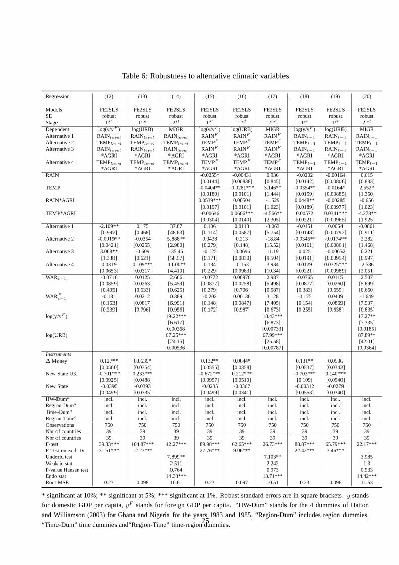
Table 6: Robustness to alternative climatic variables

Regression (12) (13) (14) (15) (16) (17) (18) (19) (20)

Models FE2SLS FE2SLS FE2SLS FE2SLS FE2SLS FE2SLS FE2SLS FE2SLS FE2SLSSE robust robust robust robust robust robust robust robust robustStage 1st 1nd 2st 1st 1nd 2nd 1st 1st 2nd

Dependent log(y/yF ) log(URB) MIGR log(y/yF ) log(URB) MIGR log(y/yF ) log(URB) MIGRAlternative 1 RAINlevel RAINlevel RAINlevel RAINF RAINF RAINF RAINt−1 RAINt−1 RAINt−1

Alternative 2 TEMPlevel TEMPlevel TEMPlevel TEMPF TEMPF TEMPF TEMPt−1 TEMPt−1 TEMPt−1

Alternative 3 RAINlevel RAINlevel RAINlevel RAINF RAINF RAINF RAINt−1 RAINt−1 RAINt−1

*AGRI *AGRI *AGRI *AGRI *AGRI *AGRI *AGRI *AGRI *AGRIAlternative 4 TEMPlevel TEMPlevel TEMPlevel TEMPF TEMPF TEMPF TEMPt−1 TEMPt−1 TEMPt−1

*AGRI *AGRI *AGRI *AGRI *AGRI *AGRI *AGRI *AGRI *AGRIRAIN -0.0255* -0.00431 0.936 -0.0202 -0.00164 0.615

[0.0144] [0.00838] [0.845] [0.0142] [0.00806] [0.883]TEMP -0.0404** -0.0281*** 3.146** -0.0354** -0.0164* 2.552*

[0.0180] [0.0101] [1.444] [0.0159] [0.00885] [1.350]RAIN*AGRI 0.0539*** 0.00504 -1.529 0.0448** -0.00285 -0.656

[0.0197] [0.0101] [1.023] [0.0189] [0.00977] [1.023]TEMP*AGRI -0.00646 0.0606*** -4.566** 0.00572 0.0341*** -4.278**

[0.0304] [0.0140] [2.305] [0.0221] [0.00965] [1.925]Alternative 1 -2.109** 0.175 37.87 0.106 0.0113 -3.063 -0.0151 0.0054 -0.0861

[0.997] [0.468] [48.63] [0.114] [0.0587] [5.754] [0.0148] [0.00792] [0.911]Alternative 2 -0.0919** -0.0354 5.888** 0.0438 0.213 -18.84 -0.0345** -0.0174** 2.282

[0.0421] [0.0255] [2.980] [0.279] [0.148] [15.52] [0.0161] [0.00861] [1.468]Alternative 3 3.068** -0.609 -35.45 -0.125 -0.0696 11.19 0.025 -0.00652 0.221

[1.338] [0.621] [58.57] [0.171] [0.0830] [9.504] [0.0191] [0.00954] [0.997]Alternative 4 0.0319 0.109*** -11.00** 0.134 -0.153 3.934 0.0129 0.0325*** -2.586

[0.0653] [0.0317] [4.410] [0.229] [0.0983] [10.34] [0.0221] [0.00989] [2.051]WARt−1 -0.0716 0.0125 2.666 -0.0772 0.00976 2.987 -0.0765 0.0115 2.507

[0.0859] [0.0263] [5.459] [0.0877] [0.0258] [5.498] [0.0877] [0.0260] [5.699][0.405] [0.633] [0.625] [0.379] [0.706] [0.587] [0.383] [0.659] [0.660]

WARF

t−1-0.181 0.0212 0.389 -0.202 0.00136 3.128 -0.175 0.0409 -1.649[0.153] [0.0817] [6.991] [0.148] [0.0847] [7.405] [0.154] [0.0869] [7.937][0.239] [0.796] [0.956] [0.172] [0.987] [0.673] [0.255] [0.638] [0.835]

log(y/yF ) 19.22*** 18.43*** 17.27**[6.617] [6.873] [7.335]

[0.00368] [0.00733] [0.0185]log(URB) 67.25*** 67.99*** 87.89**

[24.15] [25.58] [42.01][0.00536] [0.00787] [0.0364]

Instruments∆ Money 0.127** 0.0639* 0.132** 0.0644* 0.131** 0.0506

[0.0560] [0.0354] [0.0555] [0.0358] [0.0537] [0.0342]New State UK -0.701*** 0.233*** -0.672*** 0.212*** -0.703*** 0.140***

[0.0925] [0.0488] [0.0957] [0.0510] [0.109] [0.0540]New State -0.0395 -0.0393 -0.0235 -0.0367 -0.00312 -0.0279

[0.0499] [0.0335] [0.0499] [0.0341] [0.0553] [0.0340]HW-Duma incl. incl. incl. incl. incl. incl. incl. incl. incl.Region-Duma incl. incl. incl. incl. incl. incl. incl. incl. incl.Time-Duma incl. incl. incl. incl. incl. incl. incl. incl. incl.Region-Timea incl. incl. incl. incl. incl. incl. incl. incl. incl.Observations 750 750 750 750 750 750 750 750 750Nbr of countries 39 39 39 39 39 39 39 39 39Nbr of countries 39 39 39 39 39 39 39 39 39F-test 39.33*** 104.87*** 42.27*** 89.98*** 62.65*** 26.73*** 88.87*** 65.79*** 22.17***F-Test on excl. IV 31.51*** 12.23*** 27.76*** 9.06*** 22.42*** 3.46***Underid test 7.899** 7.103** 3.985Weak id stat 2.511 2.242 1.3P-value Hansen test 0.764 0.973 0.933Endo stat 14.33*** 13.71*** 14.42***Root MSE 0.23 0.098 10.61 0.23 0.097 10.51 0.23 0.096 11.53

* significant at 10%; ** significant at 5%; *** significant at 1%. Robust standard errors are in square brackets.y stands

for domestic GDP per capita,yF stands for foreign GDP per capita. “HW-Dum” stands for the 4 dummies of Hatton

and Williamson (2003) for Ghana and Nigeria for the years 1983 and 1985, “Region-Dum” includes region dummies,

“Time-Dum” time dummies and“Region-Time” time-region dummies.25

Table 7: Robustness to alternative economic variables (Part1)

Regression (21) (22) (23) (24) (25) (26) (27) (28) (29)

Models FE2SLS FE2SLS FE2SLS FE2SLS FE2SLS FE2SLS FE2SLS FE2SLS FE2SLSSE robust robust robust robust robust robust robust robust robustStage 1st 1nd 2st 1st 1nd 2nd 1st 1st 2nd

Dependent log(y/yF ) log(URB) MIGR log(y/yF ) log(URB) MIGR log(y/yF ) log(URB) MIGRAlternative GDP per GDP per GDP per Chain Chain Chain Colony Colony Colonylog(y/yF ) worker worker worker Trans. Trans. Trans.RAIN -0.0203 -0.00332 0.944 -0.0229 -0.00332 0.846 -0.0197 -0.00332 0.899

[0.0135] [0.00832] [0.894] [0.0139] [0.00832] [0.834] [0.0137] [0.00832] [0.957]TEMP -0.0416*** -0.0204** 3.095** -0.0429*** -0.0204** 2.846** -0.0384** -0.0204** 3.221**

[0.0149] [0.00876] [1.362] [0.0153] [0.00876] [1.242] [0.0149] [0.00876] [1.511]RAIN*AGRI 0.0421** 0.00162 -1.437 0.0493*** 0.00162 -1.264 0.0448** 0.00162 -1.33

[0.0183] [0.00997] [1.027] [0.0187] [0.00997] [0.939] [0.0186] [0.00997] [1.095]TEMP*AGRI 0.0177 0.0455*** -4.496** 0.00808 0.0455*** -4.262** -0.00491 0.0455*** -4.782**

[0.0212] [0.00980] [1.841] [0.0218] [0.00980] [1.697] [0.0216] [0.00980] [2.062]WARt − 1 -0.0669 0.0104 3.413 -0.0746 0.0104 3.026 -0.0748 0.0104 3.055

[0.0868] [0.0259] [6.238] [0.0877] [0.0259] [5.723] [0.0882] [0.0259] [6.091]WARF

t−1t − 1 -0.137 0.02 1.054 -0.183 0.02 0.904 -0.205 0.02 1.611[0.142] [0.0850] [7.670] [0.150] [0.0850] [7.213] [0.147] [0.0850] [8.448]

Alternative 29.66*** 21.75*** 24.60**log(y/yF ) [10.29] [7.269] [9.575]log(URB) 65.19*** 67.69*** 85.80**

[24.59] [24.17] [34.82]Instruments∆ Money 0.0987* 0.0596* 0.129** 0.0596* 0.0618 0.0596*

[0.0519] [0.0350] [0.0563] [0.0350] [0.0541] [0.0350]New State UK -0.428*** 0.230*** -0.641*** 0.230*** -0.616*** 0.230***

[0.0820] [0.0484] [0.0891] [0.0484] [0.0872] [0.0484]New State -0.0451 -0.0362 -0.0258 -0.0362 -0.101** -0.0362

[0.0554] [0.0338] [0.0505] [0.0338] [0.0480] [0.0338]HW-Duma incl. incl. incl. incl. incl. incl. incl. incl. incl.Region-Duma incl. incl. incl. incl. incl. incl. incl. incl. incl.Time-Duma incl. incl. incl. incl. incl. incl. incl. incl. incl.Region-Timea incl. incl. incl. incl. incl. incl. incl. incl. incl.Observations 750 750 750 750 750 750 750 750 750Number of countries 39 39 39 39 39 39 39 39 39F-test 95.46*** 65.79*** 270.96*** 90.41*** 65.79*** 22.20*** 32.49*** 65.79*** 13.71***F-Test on excl. IV 23.31*** 12.99*** 30.59*** 12.99*** 35.13*** 12.99***Underid test 11.82*** 7.665** 8.265**Weak id stat 0.00271 0.0217 0.016P-value Hansen test 0.746 0.891 0.487Endo stat 14.67*** 14.56*** 13.08***Root MSE 0.23 0.097 11.75 0.23 0.097 10.85 0.23 0.097 12.1

* significant at 10%; ** significant at 5%; *** significant at 1%. Robust standard errors are in square brackets.y stands

for domestic GDP per capita,yF stands for foreign GDP per capita. “HW-Dum” stands for the 4 dummies of Hatton

and Williamson (2003) for Ghana and Nigeria for the years 1983 and 1985, “Region-Dum” includes region dummies,

“Time-Dum” time dummies and“Region-Time” time-region dummies.

26

Table 8: Robustness to alternative economic variables (Part2)

Regression (30) (31) (32) (33) (34) (35) (36) (37) (38)

Models FE2SLS FE2SLS FE2SLS FE2SLS FE2SLS FE2SLS FE2SLS FE2SLS FE2SLSSE robust robust robust robust robust robust robust robust robustStage 1st 1nd 2st 1st 1nd 2nd 1st 1st 2nd

Dependent log(y/yF ) log(URB) MIGR log(y/yF ) log(URB) MIGR log(y/yF ) log(URB) MIGRa

Alternative log(y/yF ) Common Common Common Contiguity Contiguity Contiguity Linguistic Linguistic LinguisticColony Colony Colony proximity proximity proximity

RAIN -0.0454*** -0.00332 1.512 -0.0292* -0.00332 0.943 -0.0172 -0.00332 0.748[0.0151] [0.00832] [1.112] [0.0173] [0.00832] [0.924] [0.0152] [0.00832] [0.896]

TEMP -0.0470*** -0.0204** 3.376** -0.019 -0.0204** 2.471** -0.0381** -0.0204** 2.965**[0.0172] [0.00876] [1.610] [0.0231] [0.00876] [1.249] [0.0173] [0.00876] [1.408]

RAIN*AGRI 0.0575*** 0.00162 -1.624 0.0497** 0.00162 -1.166 0.0446** 0.00162 -1.133[0.0192] [0.00997] [1.161] [0.0227] [0.00997] [1.027] [0.0198] [0.00997] [1.017]

TEMP*AGRI -0.0096 0.0455*** -4.568** -0.0314 0.0455*** -3.910** -0.0125 0.0455*** -4.429**[0.0219] [0.00980] [2.015] [0.0273] [0.00980] [1.734] [0.0232] [0.00980] [1.919]

WARt − 1 -0.0225 0.0104 1.788 -0.0802 0.0104 2.853 -0.104 0.0104 3.408[0.0887] [0.0259] [6.147] [0.0961] [0.0259] [5.714] [0.0925] [0.0259] [5.813]

WARF

t−1t − 1 -0.145 0.02 0.152 -0.23 0.02 1.192 -0.221 0.02 1.231[0.163] [0.0850] [9.419] [0.196] [0.0850] [7.884] [0.154] [0.0850] [7.917]

Alternative 24.35** 19.30*** 20.61**log(y/yF ) [9.572] [7.225] [8.007]log(URB) 83.56** 77.16** 80.91**

[34.38] [30.38] [32.96]Instruments∆ Money 0.0685 0.0596* 0.116** 0.0596* 0.0974* 0.0596*

[0.0520] [0.0350] [0.0579] [0.0350] [0.0527] [0.0350]New State UK -0.608*** 0.230*** -0.827*** 0.230*** -0.804*** 0.230***

[0.0906] [0.0484] [0.0901] [0.0484] [0.0906] [0.0484]New State -0.101** -0.0362 -0.0204 -0.0362 -0.0248 -0.0362

[0.0488] [0.0338] [0.0572] [0.0338] [0.0487] [0.0338]HW-Duma incl. incl. incl. incl. incl. incl. incl. incl. incl.Region-Duma incl. incl. incl. incl. incl. incl. incl. incl. incl.Time-Duma incl. incl. incl. incl. incl. incl. incl. incl. incl.Region-Timea incl. incl. incl. incl. incl. incl. incl. incl. incl.Observations 750 750 750 750 750 750 750 750 750Number of countries 39 39 39 39 39 39 39 39 39F-test 285.58*** 65.79*** 50.79*** 28.66*** 65.79*** 19.31*** 65.24*** 65.79*** 25.55***F-Test on excl. IV 31.88*** 12.99*** 55.21*** 12.99*** 41.87*** 12.99***Underid test 8.455** 7.548** 6.933**Weak id stat 0.0146 0.023 0.0312P-value Hansen test 0.5 0.857 0.803Endo stat 13.001*** 14.34*** 14.4***Root MSE 0.239 0.097 12.48 0.27 0.097 11.36 0.241 0.097 11.48

* significant at 10%; ** significant at 5%; *** significant at 1%. Robust standard errors are in square brackets.y stands

for domestic GDP per capita,yF stands for foreign GDP per capita. “HW-Dum” stands for the 4 dummies of Hatton

and Williamson (2003) for Ghana and Nigeria for the years 1983 and 1985, “Region-Dum” includes region dummies,

“Time-Dum” time dummies and“Region-Time” time-region dummies.

27

Table 9: Robustness to the addition or omission of control variables

Regression (39) (40) (41) (42) (43) (44) (45) (46) (47)

Models FE2SLS FE2SLS FE2SLS FE2SLS FE2SLS FE2SLS FE2SLS FE2SLS FE2SLSSE robust robust robust robust robust robust robust robust robustStage 1st 2nd 1st 1st 2nd 2nd 1st 1st 2nd

Dependent log(y/yF ) log(URB) MIGR log(y/yF ) log(URB) MIGR log(y/yF ) log(URB) MIGRVariable

Addition ACP ACP ACP Density Density DensityOmission No Conflict No Conflict No ConflictRAIN -0.0232* -0.0033 0.882 -0.0229 -0.00332 0.849 -0.00819 -0.00133 0.484

[0.0137] [0.00831] [0.822] [0.0141] [0.00831] [0.844] [0.0143] [0.00797] [0.828]TEMP -0.0426*** -0.0204** 2.851** -0.0435*** -0.0203** 2.858** -0.0387** -0.0200** 2.636**

[0.0152] [0.00877] [1.228] [0.0153] [0.00876] [1.244] [0.0155] [0.00875] [1.221]RAIN*AGRI 0.0498*** 0.00159 -1.367 0.0473** 0.00191 -1.187 0.0378** -0.000235 -1.271

[0.0185] [0.00996] [0.927] [0.0184] [0.00999] [0.908] [0.0188] [0.0101] [0.980]TEMP*AGRI 0.0106 0.0452*** -4.161** 0.00614 0.0458*** -4.219** 0.0134 0.0480*** -4.118**

[0.0214] [0.00983] [1.652] [0.0217] [0.00975] [1.696] [0.0219] [0.0101] [1.660]WARt − 1 -0.0742 0.0104 3.211 -0.0947 0.0039 5.013

[0.0877] [0.0259] [5.818] [0.0904] [0.0251] [6.421]WARF

t−1t − 1 -0.182 0.02 1.355 -0.26 0.00357 6.48[0.150] [0.0851] [7.177] [0.164] [0.0829] [7.486]

Addition 0.177* -0.0163 -3.697 0.00310*** 0.000668 -0.140**[0.1000] [0.0354] [2.936] [0.000754] [0.000590] [0.0606]

log(y/yF ) 23.86*** 21.63*** 31.00***[8.079] [7.243] [10.05]

log(URB) 63.82*** 68.50*** 55.82***[22.78] [24.37] [19.37]

Instruments∆ Money 0.128** 0.0598* 0.129** 0.0598* 0.119** 0.0567

[0.0541] [0.0350] [0.0557] [0.0350] [0.0533] [0.0358]New State UK -0.615*** 0.228*** -0.646*** 0.231*** -0.408*** 0.275***

[0.0929] [0.0489] [0.0897] [0.0481] [0.0975] [0.0613]New State 0.0843 -0.0467 -0.0292 -0.0362 -0.0469 -0.0395

[0.0892] [0.0380] [0.0508] [0.0337] [0.0514] [0.0342]HW-Duma incl. incl. incl. incl. incl. incl. incl. incl. incl.Region-Duma incl. incl. incl. incl. incl. incl. incl. incl. incl.Time-Duma incl. incl. incl. incl. incl. incl. incl. incl. incl.Region-Timea incl. incl. incl. incl. incl. incl. incl. incl. incl.Observations 750 750 750 750 750 750 750 735 735Number of countries 39 39 39 39 39 39 39 39 39Number of countries 39 39 39 39 39 39 39 39 39F-test 85.57*** 68.72*** 56.11*** 64.18*** 64.98*** 595.00*** 61.10 54.18*** 3512.28***F-Test on excl. IV 17.56*** 9.22*** 31.07*** 13.18*** 14.25*** 9.06***Underid test 7.773** 7.661** 13.59***Weak id stat 2.56 2.449 4.822P-value Hansen test 0.535 0.869 0.731Endo stat 13.94*** 14.41*** 14.45***Root MSE 0.23 0.097 10.87 0.23 0.097 10.89 0.23 0.098 11.3

* significant at 10%; ** significant at 5%; *** significant at 1%. Robust standard errors are in square brackets.y stands

for domestic GDP per capita,yF stands for foreign GDP per capita. “HW-Dum” stands for the 4 dummies of Hatton

and Williamson (2003) for Ghana and Nigeria for the years 1983 and 1985, “Region-Dum” includes region dummies,

“Time-Dum” time dummies and“Region-Time” time-region dummies.

28

Table 10: Robustness with alternative OECD dataset

Regression (48) (49) (50) (51) (52) (53) (54) (55) (56)

Models FE FE FE2SLS FE2SLS FE2SLS FE2SLS FE2SLS FE2SLS FE2SLS

SE robust robust robust robust robust robust robust robust robustStage 1st 2nd 1st 2st 1nd 1st 2st

Dependent MIGR MIGR log(y/yF ) MIGR log(y/yF ) MIGR log(y/yF ) log(URB) MIGRVariable

log(y/yF ) -2.863** -2.824** -19.73* -12.67* -10.06**[1.354] [1.357] [10.88] [7.540] [5.022]

RAIN 0.00869 -0.0247*** -0.463 -0.0232*** -0.00424 -0.0232*** -0.00683** 0.0459[0.239] [0.00570] [0.410] [0.00576] [0.281] [0.00577] [0.00316] [0.232]

RAIN*AGRI -0.155 0.0205*** 0.377 0.0173** -0.0885 0.0186** 0.00509 -0.126[0.236] [0.00739] [0.404] [0.00738] [0.241] [0.00740] [0.00421] [0.198]

TEMP 0.349 -0.0394*** -0.286 -0.0349*** -0.0717 -0.0336*** -0.0133*** -0.00111[0.292] [0.00584] [0.559] [0.00603] [0.388] [0.00602] [0.00336] [0.347]

TEMP*AGRI -0.383 -0.00396 -0.426 -0.00637 -0.386 -0.00823 0.0236*** -0.333[0.345] [0.00772] [0.396] [0.00772] [0.333] [0.00771] [0.00406] [0.323]

log(Distance) -2.143 -2.143 -0.00791 -2.568[2.368] [2.365] [0.0445] [2.580]

WARt−1 0.631 0.653 0.00466 0.886 -0.00294 0.511 -0.00229 0.00715 0.529[1.225] [1.216] [0.0231] [1.221] [0.0238] [1.144] [0.0237] [0.00857] [1.149]

log(URB) -1.543[2.511]

Instruments∆ Money 0.0277*** 0.0296*** 0.159*** 0.0612***

[0.00906] [0.0110] [0.0283] [0.0137]New State -0.00957 -0.00399

[0.0332] [0.0179]Constant 22.93 22.84

[22.83] [22.83]

αi Incl. Incl. Incl. Incl. Incl. Incl. Incl.αj Incl. Incl. Incl. Incl. Incl. Incl. Incl.αij Incl. Incl.HW-Duma Incl. Incl. Incl. Incl. Incl. Incl. Incl. Incl. Incl.Region-Duma Incl. Incl. Incl. Incl. Incl. Incl. Incl. Incl. Incl.Time-Duma Incl. Incl. Incl. Incl. Incl. Incl. Incl. Incl. Incl.Region-Timea Incl. Incl. Incl. Incl. Incl. Incl. Incl. Incl. Incl.Observations 4’959 4’959 4’503 4’503 4’463 4’463 4’463 4’463 4’463F test 9172*** 37774*** 599*** 3.90*** 593*** 228*** 151***F-Test on excl. IV 9.33*** 7.31*** 13.85*** 39.27***P-value Hansen 0.0989Underid test 14.75*** 11.49*** 26.32***Root MSE 7.621 7.622 0.210 8.293 0.203 5.834 0.203 0.0911 5.742

* significant at 10%; ** significant at 5%; *** significant at 1%. Robust standard errors are in square brackets.y stands

for GDP per capita in migrants’ origin countries,yF stands for GDP per capita in destination countries. “HW-Dum”

stands for the 4 dummies of Hatton and Williamson (2003) for Ghana and Nigeria for the years 1983 and 1985, “Region-

Dum” includes region dummies, “Time-Dum” time dummies and “Region-Time” time-region dummies. Efficiency of

regressions (16)-(18) have been strengthened by introducing the square of the money supply to make the instruments

stronger. Otherwise, the second-stage is less precise due to the instrument weakness in such a setting. Angrist-Pischke

multivariate F test of excluded instruments for regression(54)-(56). R-squared not shown, because, in the case of 2SLS/IV,

it is not an appropriate measure of the goodness of fit and has no statistical meaning (see www.stata.com).

29

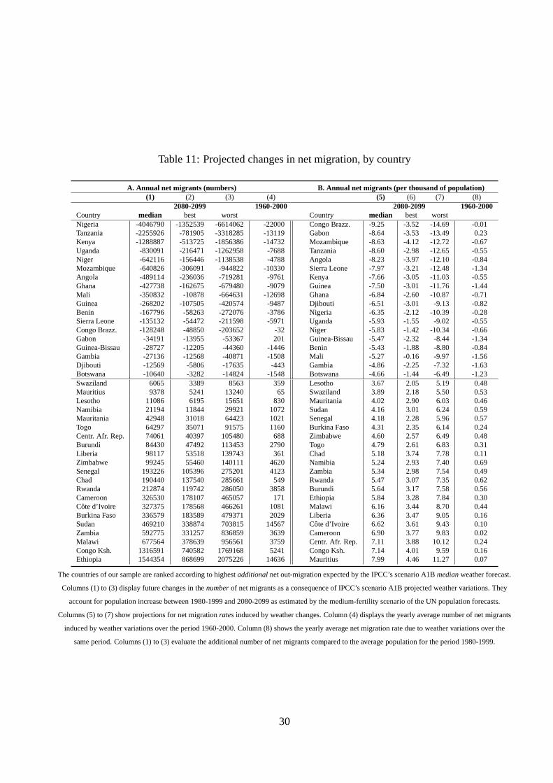
Table 11: Projected changes in net migration, by country

A. Annual net migrants (numbers) B. Annual net migrants (per thousand of population)(1) (2) (3) (4) (5) (6) (7) (8)

2080-2099 1960-2000 2080-2099 1960-2000Country median best worst Country median best worstNigeria -4046790 -1352539 -6614062 -22000 Congo Brazz. -9.25 -3.52 -14.69 -0.01Tanzania -2255926 -781905 -3318285 -13119 Gabon -8.64 -3.53 -13.49 0.23Kenya -1288887 -513725 -1856386 -14732 Mozambique -8.63 -4.12 -12.72 -0.67Uganda -830091 -216471 -1262958 -7688 Tanzania -8.60 -2.98 -12.65 -0.55Niger -642116 -156446 -1138538 -4788 Angola -8.23 -3.97 -12.10 -0.84Mozambique -640826 -306091 -944822 -10330 Sierra Leone -7.97 -3.21 -12.48 -1.34Angola -489114 -236036 -719281 -9761 Kenya -7.66 -3.05 -11.03 -0.55Ghana -427738 -162675 -679480 -9079 Guinea -7.50 -3.01 -11.76 -1.44Mali -350832 -10878 -664631 -12698 Ghana -6.84 -2.60 -10.87 -0.71Guinea -268202 -107505 -420574 -9487 Djibouti -6.51 -3.01 -9.13 -0.82Benin -167796 -58263 -272076 -3786 Nigeria -6.35 -2.12 -10.39 -0.28Sierra Leone -135132 -54472 -211598 -5971 Uganda -5.93 -1.55 -9.02 -0.55Congo Brazz. -128248 -48850 -203652 -32 Niger -5.83 -1.42 -10.34 -0.66Gabon -34191 -13955 -53367 201 Guinea-Bissau -5.47 -2.32 -8.44 -1.34Guinea-Bissau -28727 -12205 -44360 -1446 Benin -5.43 -1.88 -8.80 -0.84Gambia -27136 -12568 -40871 -1508 Mali -5.27 -0.16 -9.97 -1.56Djibouti -12569 -5806 -17635 -443 Gambia -4.86 -2.25 -7.32 -1.63Botswana -10640 -3282 -14824 -1548 Botswana -4.66 -1.44 -6.49 -1.23Swaziland 6065 3389 8563 359 Lesotho 3.67 2.05 5.19 0.48Mauritius 9378 5241 13240 65 Swaziland 3.89 2.18 5.50 0.53Lesotho 11086 6195 15651 830 Mauritania 4.02 2.90 6.03 0.46Namibia 21194 11844 29921 1072 Sudan 4.16 3.01 6.24 0.59Mauritania 42948 31018 64423 1021 Senegal 4.18 2.28 5.96 0.57Togo 64297 35071 91575 1160 Burkina Faso 4.31 2.35 6.14 0.24Centr. Afr. Rep. 74061 40397 105480 688 Zimbabwe 4.60 2.57 6.49 0.48Burundi 84430 47492 113453 2790 Togo 4.79 2.61 6.83 0.31Liberia 98117 53518 139743 361 Chad 5.18 3.74 7.78 0.11Zimbabwe 99245 55460 140111 4620 Namibia 5.24 2.93 7.40 0.69Senegal 193226 105396 275201 4123 Zambia 5.34 2.98 7.54 0.49Chad 190440 137540 285661 549 Rwanda 5.47 3.07 7.35 0.62Rwanda 212874 119742 286050 3858 Burundi 5.64 3.17 7.58 0.56Cameroon 326530 178107 465057 171 Ethiopia 5.84 3.28 7.84 0.30Côte d’Ivoire 327375 178568 466261 1081 Malawi 6.16 3.44 8.70 0.44Burkina Faso 336579 183589 479371 2029 Liberia 6.36 3.47 9.05 0.16Sudan 469210 338874 703815 14567 Côte d’Ivoire 6.62 3.61 9.43 0.10Zambia 592775 331257 836859 3639 Cameroon 6.90 3.77 9.83 0.02Malawi 677564 378639 956561 3759 Centr. Afr. Rep. 7.11 3.88 10.12 0.24Congo Ksh. 1316591 740582 1769168 5241 Congo Ksh. 7.14 4.01 9.59 0.16Ethiopia 1544354 868699 2075226 14636 Mauritius 7.99 4.46 11.27 0.07

The countries of our sample are ranked according to highestadditionalnet out-migration expected by the IPCC’s scenario A1Bmedianweather forecast.

Columns (1) to (3) display future changes in thenumberof net migrants as a consequence of IPCC’s scenario A1B projected weather variations. They

account for population increase between 1980-1999 and 2080-2099 as estimated by the medium-fertility scenario of the UN population forecasts.

Columns (5) to (7) show projections for net migrationratesinduced by weather changes. Column (4) displays the yearly average number of net migrants

induced by weather variations over the period 1960-2000. Column (8) shows the yearly average net migration rate due to weather variations over the

same period. Columns (1) to (3) evaluate the additional number of net migrants compared to the average population for the period 1980-1999.

30

ISSN 1379-244X D/2011/3082/034