Embed Size (px)
Citation preview

University of Nebraska at OmahaDigitalCommons@UNO
Student Work
12-2013
The Importance of Mapping to the NextGeneration Retinal ProsthesisJonathan GesellUniversity of Nebraska at Omaha
Follow this and additional works at: https://digitalcommons.unomaha.edu/studentwork
Part of the Computer Sciences Commons
This Thesis is brought to you for free and open access byDigitalCommons@UNO. It has been accepted for inclusion in StudentWork by an authorized administrator of DigitalCommons@UNO. Formore information, please contact [email protected].
Recommended CitationGesell, Jonathan, "The Importance of Mapping to the Next Generation Retinal Prosthesis" (2013). Student Work. 2895.https://digitalcommons.unomaha.edu/studentwork/2895

The Importance of Mapping to the Next Generation Retinal Prosthesis
A Thesis
Presented to the
Department of Computer Science
and the
Faculty of the Graduate College
University of Nebraska
In Partial Fulfillment
Of the Requirements for the Degree
Master of Science
University of Nebraska at Omaha
By
Jonathan Gesell
December 2013
Supervisory Committee:
Dr. Mahadevan Subramaniam
Dr. Parvathi Chundi
Dr. Eyal Margalit

All rights reserved
INFORMATION TO ALL USERSThe quality of this reproduction is dependent upon the quality of the copy submitted.
In the unlikely event that the author did not send a complete manuscriptand there are missing pages, these will be noted. Also, if material had to be removed,
a note will indicate the deletion.
Microform Edition © ProQuest LLC.All rights reserved. This work is protected against
unauthorized copying under Title 17, United States Code
ProQuest LLC.789 East Eisenhower Parkway
P.O. Box 1346Ann Arbor, MI 48106 - 1346
UMI 1555143
Published by ProQuest LLC (2014). Copyright in the Dissertation held by the Author.
UMI Number: 1555143
The Importance of Mapping to the Next Generation Retinal Prosthesis
JONATHAN GESELL, M.S.
University of Nebraska, 2013
Advisor: Dr. Mahadevan Subramaniam
Abstract
Evolutionarily, human beings have come to rely on vision more than any other
sense, and with the prevalence of visual-oriented stimuli and the necessity of computers
and visual media in everyday activities, this can be problematic. Therefore, the develop-
ment of an accurate and fast retinal prosthesis to restore the lost portions of the visual field
for those with specific types of vision loss is vital, but current methodologies are extremely
limited in scope. All current models use a spatio-temporal filter (ST), which uses a differ-
ence of Gaussian (DOG) to mimic the inner layers of the retina and a noisy leak and fire
integrate (NLIF) unit to simulate the optical ganglion. None of these processes show how
these filters are mapped to each other, and therefore simulate the interaction of cells with
each other in the retina.
The mapping is key to having a fast and efficient filtering method; one that will
allow for higher-resolution images with significantly less hardware, and therefore power
requirements. The focus of this thesis was streamlining this process: the first major portion
involved was applying a pipelining system to the 3D-ADoG, which showed some signifi-
cant improvement over the design by Eckmiller. The major contribution was the mapping
process: three mapping schemes were tried, and there was a significant difference found
between them. While none of the models met the timing requirements, the ratios for
speedups seen between the methods was significant.
Despite the speedups and potential power savings, none of the other papers made
specific mention of using any mapping schemes, nor how they improve both the speed and
quality of the output images. The closest reference: a very vague reference to the amount
of overlap as a tunable feature. Nevertheless, this is a key feature to developing the next
generation prosthesis, and the manner in which the output from the ST filter bank is mapped
seems to have a significant effect on speed, quality, and efficiency of the entire system as
a whole.

iii
ACKNOWLEDGEMENTS
Without a lot of help, none of this would have been possible.
First: Dr. Subramaniam and Dr. Chundi, for keeping me on track, for all of the as-sistance, both technical and personal, and for your patience and guidance.
To my family, for their support and encouragement during this long process.
To Sarah, for being a beacon to me, every time things got rough, and for listening to all the ramblings, rants and raves as this went on.
To the RooE202 crew, who allowed me an outlet, and kept me sane, while keep-ing me on track to get it done.
iv
TABLE OF CONTENTS
CHAPTER 1: INTRODUCTION .................................................................................................................... 1
INTRODUCTION ............................................................................................................................... 1 CURRENT MODELS .............................................................................................................................. 3 IMPROVEMENTS ON THE EXISTING MODELS. ............................................................................................. 6
CHAPTER 2: THE BIOLOGICAL PROCESS OF HUMAN VISION ..................................................................... 9
CELLS ............................................................................................................................................... 9 SIMULATING CELL INTERACTIONS ......................................................................................................... 18
CHAPTER 3: ST FILTERS ........................................................................................................................... 20
GAUSSIAN FILTERS ............................................................................................................................ 20 GAUSSIAN RADIUS ............................................................................................................................ 22 3-DIMENSIONAL ADAPTIVE DIFFERENCE OF GAUSSIAN ............................................................................. 23 BASICS OF THIS IMPLEMENTATION ....................................................................................................... 26
CHAPTER 4: PIPELINING ................................................................................................................ 28
BASICS OF PIPELINING ....................................................................................................................... 28 IMPLEMENTATION IN THIS PROJECT ...................................................................................................... 29
CHAPTER 5: MAPPINGS ................................................................................................................... 35
MAPPING TYPES ............................................................................................................................... 35 1-TO-1 MAPPING ............................................................................................................................. 36 MANY-TO-MANY MAPPING ............................................................................................................... 39 MAPPINGS IMPLEMENTATIONS ............................................................................................................ 41
CHAPTER 6: TIMING AND MAPPING INTERACTIONS .............................................................................. 44
TIMING FOR ORIGINAL DESIGNS .......................................................................................................... 44 TIMING FOR CURRENT DESIGNS ........................................................................................................... 47
CHAPTER 7: IMPLEMENTATION ARCH ....................................................................................... 52
ORIGINAL DESIGN ........................................................................................................................ 52 TECHNICAL SPECIFICATIONS ................................................................................................................ 52 HISTORICAL MODELS ......................................................................................................................... 52 FINAL MODELS ................................................................................................................................. 65
CHAPTER 8: CONCLUSIONS AND FUTURE WORK .................................................................................... 76
CONCLUSIONS .................................................................................................................................. 76 FUTURE WORK ................................................................................................................................. 78
APPENDIX A: WORKS CITED ...................................................................................................................... I
APPENDIX B: ORIGINAL CODE .................................................................................................................. II
B.1. ORIGINAL 9X9 PROTOTYPE.................................................................................................................... II B.2. FIRST FUNCTIONAL PROTOTYPE .............................................................................................................. V B.3. SECOND FUNCTIONAL PROTOTYPE.......................................................................................................... X
v
APPENDIX C: ORIGINAL RADIUS CODE .................................................................................................. XIV
C.1. ORIGINAL VERSION .......................................................................................................................... XIV C.2. UPDATED VERSION.......................................................................................................................... XVIII
APPENDIX D: ORIGINAL MULTICORE CODE ......................................................................................... XXIII
APPENDIX E: CURRENT CODE ............................................................................................................ XXXIII
E.1. MASTER CONTROLL PROGRAM ......................................................................................................... XXXIII E.2. 1 : 1 RATIO..................................................................................................................................... XLV E.3. MANY : 1 RATIO ............................................................................................................................. XLIX E.4. MANY : MANY RATIO USING MEAN ...................................................................................................... LIII E.5. MANY : MANY RATIO USING NEAREST NEIGHBOR ................................................................................... LVII
vi
LIST OF FIGURES/TABLES
FIG 1: FLOWCHART SHOWING THE PIPELINING SYSTEM USED WITH TIMING.................................................... 31 FIG 2: DIAGRAM OF 1-TO-1 MAPPING SCHEME USED IN THIS PROJECT. ......................................................................... 37 FIG 3: MANY-TO-1 MAPPING SCHEME USED IN THIS PROJECT. ............................................................................ 38 FIG 4: THE MANY-TO-MANY MAPPING SCHEME USED IN THIS PROJECT. ....................................................................... 40 FIG 5: TABLES SHOWING THE ST FILTER PROCESS AT ITS SIMPLEST. .............................................................. 54 FIG 6: THE ORIGINAL "LENA" IMAGE. ............................................................................................................ 57 FIG 7: "LENA" AFTER THE ORIGINAL ST FILTER PROCESS. ............................................................................................ 58 FIG 8: "LENA" AFTER THE IMPROVED ST FILTER PROCESS, WITH RADIUS FUNCTION ADDED. .............................................. 60 FIG 9: "LENA" AFTER THE IMPROVED ST FILTER PROCESS WITH BOTH RADIUS AND OVERLAP ADDED. ................................... 61 FIG 10: "LENA" AFTER A RARE, SUCCESSFUL RUN OF THE MULTI-CORE IMAGE, PRE-STALLING FIX. ....................................... 63 FIG 11: "LENA" SHOWING THE MORE COMMON RESULT OF THE MULTI-CORE RUNS, WHEN THEY COMPLETED. ..................... 64 FIG 12: 1-TO-1 FINAL OUTPUT FOR "LENA." ................................................................................................... 68 FIG 13: MANY-TO-1 FINAL OUTPUT FOR "LENA." ........................................................................................... 70 FIG 14: MANY-TO-MANY FINAL OUTPUT FOR "LENA" USING THE MEAN TO RECONSTRUCT THE IMAGE DATA
POST-FILTERING. ................................................................................................................................... 72
1
CHAPTER 1: Introduction
Introduction
The process by which humans see is a combination of processes that occur in both
the eye and the visual cortex of the brain, which is to say that while there is comprehen-
sion of much of the process, much of it is also speculation. While trying to model any
process in visual cortex in real time, and with any degree of accuracy is very difficult, if
not nigh impossible, due to the limitations on computer hardware of the current genera-
tion, it is possible to accurately model the part of this process that occurs within the eye,
as these cell processes are fairly well-understood. In order to accomplish this, and in or-
der for such a model to make sense, it is necessary to understand at a very finely detailed
level precisely what is going on in the eye itself, and how these cells interact to send the
impulses to the brain.
Before discussion on this topic may begin, it is important to note that there are
two different major types of photoreceptors in the eye: rods and cones. These cells are
primarily responsible for light and shadow, as well as edge detection (rods) and color de-
tection (cones). These interact with other cells in the membrane to send a signal along
the pathway to the visual cortex, which then interprets this data as vision. To clarify, the
cells themselves do not convey information such as color or movement, but rather that, as
currently understood, the brain deduces that information based on the signals received
from the optical ganglion.
The first challenge is determining how to replace the functionality of these cells,
as in the particular ailments of the eye that are focused on in current generation retinal
2
prostheses, these cells are destroyed utterly and do not grow back. While more detail will
be given regarding the precise functioning of these cells, the short answer to this chal-
lenge is that the resulting images are almost a hybrid of the types of vision provided by
each cell: they relay information in gray-scale, like the rods, but with the attention to de-
tail of the cones. Nevertheles, as the next chapter discusses, they are closer to simulating
the much simpler rod cells than the cone cells.
This challenge becomes greater, given that the understanding of the internal biol-
ogy of human vision is relatively limited. For example, what the process is in the first
layer with a high degree of certainty, in the second layer with certainty but lacking in
terms of technical knowledge of the process, and beyond that is mostly speculation, as
this next step is feeding the visual data directly into the brain. Therefore, the next deter-
mination in this process is that of where the prosthesis should stop, and normal data re-
sume. As discussed later, this is entirely dependent on the degree of damage to the eye
(superficial to the retina, or deeper tissue damage. Neverheless, the models presented by
Karagoz et al and Eckmiller et al, the primary sources of information for this thesis, pre-
sent a model that would allow for bypassing of nearly the entire retina, and simulate the
ganglion directly.
Once this challenge is overcome, then a whole plethora of applications for such
vision becomes available. With these ground level, yet highly complex processes mod-
eled, this extends beyond the simpler forms of vision loss experience by those with macu-
lar degeneration and retinal pigmentosa, and into other forms of vision loss. For exam-
ple, once the optical ganglion signals are understood, it becomes possible to restore vi-
sion to those who have suffered damage to this part of their eyes, such as diabetics, or
3
those who have lost vision to some other trauma. The only issue remaining at that point
is the evidence existing that shows the brain eventually stops listening to signals from
these damaged cells, making timing of implantation for the prosthesis all the more im-
portant.
Current Models
At present, there are two models that are showing great promise in the field of hu-
man vision restoration, neither of which are complete in terms of biological functionality
of the eye: the 3-dimensional adaptive difference of Gaussian process used by Karagoz et
al [1], and the more direct spatio-temporal process used by Eckmiller et al [2]. Both of
these processes are improvements on the standard difference of Gaussian filters (ST fil-
ters) that have been widely accepted, and used almost exclusively by most current gener-
ation prosthesis [2] [1] [3] [4]. The reason for this is best put by Karagoz: “the DoG filter
based retina model does not include the non-linear transduction and adaptation which oc-
cur at ealier stages of retnal processing, [but] it describes many of the actual properties of
filtering behavior of the retina.” [1] However, there are efforts to more accurately simu-
late the functioning of a real-world retina, one of the subjects of this thesis. The first is-
sue with this is to determine what constitutes a ratio of filter to retinal cell. The next is-
sue comes with ways to improve performance of these filters to get them to perform at
the same rate as the human eye. Finally, again, comes the question of just how much is
needed in terms of depth of cell replacement.
Tunable Retinal Encoder
Eckmiller uses a two-step approach to his particular retinal prosthesis models.
The first step is the standard ST filter, a single unit of which produces result R1(t), and is
4
used to simulate the retinal domain of vision. The next step is the visual system model
(VM) that uses R1(t) at given intervals, and is used to replace the optical ganglion. This
unit produces an output only if there exists sufficient input from R1(t) to produce output
P2 in the perceptual domain, essentially simulating the brain and ganglion activity.
The issue that even Eckmiller admits is that this system works well in a static en-
vironment, but does not function as well with the subtle and persistent movements that
the human eye is constantly undergoing. In addition, they believed that it was required
that their program be written in a lower-level language, such as basic or C, in order to
produce the timings necessary to properly simulate vision: the retinal encoder module
(RE) “was implemented by program modules in C/C++ as PC simulation with an average
output of 20 frames/s and …a combination of program modules in C and in assembler”
[2]. In addition, the system used was limited to a 16x16 grid of filters, and each photo
sensor input is mapped to a very specific point, that is that they placed “the RF centers of
all 256 ST filters were evenly distributed over the inpute surface on a hexagonal grid with
about 16 centers each in the horizontal and vertical directions.” [2]
This does not solve all of the issues that are present, however, and that forms the
core of this thesis. First among these is the general mapping: this thesis attempts to ex-
plore the possibility of a more dynamic mapping scheme that will allow for higher resolu-
tion images to be used, as well as filters that are more shapped to the individual rather
than a mere grid. A second issue that is addressed by both this thesis and Karagoz et al is
that it does not compensate for the whole of the retina, as each image generally goes only
thru a single ST filter in their tests. One point of agreement, hwever, is that they do not
use a strict 1 : 1 mapping ratio, but allow for “[e]ach of the photosensor input pixels
5
could be allocated to one or more ST filters.” [2]
The 3-Dimensional Adaptive Difference of Gaussian Filter (3D-ADoG)
This model served as the basis for the versions of the filter system used in this
thesis. Karagoz et al proposed a model of the retina that went beyond the simpler, single-
layer difference of Gaussian filter that was seen in the model proposed by Eckmiller. For
example, they point out one of the major shortfalls of the Eckmiller process, that it is
done “using the trial and error techniques instead of adaptive methods. It also requires
long times.” [1] Another issue that they found was on the subjectivity of the Eckmiller
process: “The standard DoG filter based retina models introducing these disadvantagers
have user-dependent and highly parametric characteristics.” [1] That is, they do not con-
form to any standard, and must be adapted to each user, however, this is not necessarily a
negative, and is one of the goals of this paper: a more adaptive DoG that can be molded
to the user without significant changes. This is important from a medical standpoint, as
each case is unique, and a one-size fits all method is seldom useful.
The goal for Karagoz et al was to allow for the system to more closely simulate
the entire retina, up to and including the optical ganglion, even going so far as to allow
for on and off center relationships between the filters, while still using the accepted DoG
filter system. However, there as also shortcomings for this proposal. Unlike Eckmiller,
Karagoz et al do not propose any specific mapping scheme, only that there must be on
and off-center, so there must be a center and surround filtering group. This matches the
hexagonal groupings proposed by Eckmiller, though it is not directly stated. This model
serves as the basis for most of the process used in this paper, however, it is hardly the end
of the development for it. While they do not specify any particular mapping scheme,
6
there is some overlap in terms of layers, as theirs was the only system that porposed using
multiple layers of ST filters to more accurately simulate the functional retina.
Improvements on the existing models.
The improvements that are going to be explored in this thesis revolve around sev-
eral ideas regarding the assertions and mappings presented in Eckmiller et al and Karagoz
et al. The first of these assertions explored is the idea that this system can only reach de-
sired timings if a lower-level programming language, such as C or basic is used. Indeed,
while the timings that are desired were not met with the models that this thesis produced,
they do show a roadmap to how to overcome the 100ms barrier, and get down to the de-
sired 30ms run time.
The next notion that will be challenged is to lock down the radius that an ST filter
should cover. As is discussed, there are trade offs for size of the radius, allowing for
overlap between filters, and image resolution. Indeed, contrary to the initial hypothesis,
allowing for some overlap actually increased the run time under a very specific set of cir-
cumstances, but there is a limit as to how much. Eckmiller proposed a mapping scheme
that, while not clear, can be inferred to mean that there is overlap between filters: they
state that they allow overlap: “input pixels could be allocated to one or more of the ST
filters…properties of each ST filter could be modified by 11 parameters with a wide
value range (-1 to +1, 32-bit resolution)” [2], but do not specify what exactly this means.
Karagoz also does not specify the mappings used, other than that each pixel is run thru at
least 2 ST filter banks, but not how many filters per bank. This relates to the final idea
that is part of the contribution of this thesis: the mappings. The proposals by Karagoz

7
and Eckmiller et al make no mention of what sort of mapping is used between the ST fil-
ter system and the image data and and out, but based on the papers, it seems to be a sim-
ple 1:1 ratio. In other words, each pixel in is fed into only a single ST filter, and the out-
put results from the data regarding only that single pixel.
This is arguably the most important part of this thesis: the attempts at three of the
four mappings, those determined to be practical in this regards, 1-to-1, Many-to-1 and
Many-to-Many mapping schemes. This was researched for two reasons: thie first is
speed, the second to more realistically simulate the biological functioning of the retina.
These two points are more related than would initially appear, as the more overlap that
exists, the longer the process will take to run, however, the cells in the human retina also
do not exist in any sort of finite and defined isolation, as inferred by the models used in
Eckmiller and Karagoz et al.
Therefore, based on the above, the contributions of this thesis are as follows:
1) It will attempt to actually implement a functional version of the works of Ka-
ragoz et al and Eckmiller et al, built from scratch, as they provided no code
feedback 2) It will use mappings to more accurately simulate the human retina, and how
the individual ST filters will interact with each other and how they alter the
outputs for each filter, and each layer 3) To alter the parameters of each mapping to see whch mapping schemes can
effectively be used and still meet the timing requirements.
8
There was, initially, a fourth parameter, however, this was dropped due to infeasibility
within this timeframs: the use of multithreading. While this initially did show a lot of
promise, the implementation along with the other aspects were never functionially real-
ized. They are discussed here, primarily for historical reasons, and as an option for po-
tential future work.
Overall, the results showed promise: first, a successful model was created based
on a merging of the Karagoz and Eckmiller design descriptions. Second, we found that
there was a significant difference in the timings based on which mapping scheme was
chosen. Finally, there showed exceptional promise in terms of standard programming
speedups, such as pipelining and multicore, such as pipelining, and the initial attempts at
multithredding. As stated, while multithreading was never fully implemented, there was
sufficient evidence that it would allow for the breaking of the timing barrier, even using
the higher-level programming languages that were discouraged by Eckmiller.
These results are discussed in much further detail in each of the following chap-
ters, but starting with a brief introduction into the science of vision in chapter 2. After
that comes an introduction into the specifics of ST filters and the DoG process in chapter
3, followed in chapter 4 with the discussion of the main form of speedup that was made
functional: pipelining. In chapter 5 is the weight of the thesis: mappings and the mapping
schemes used, and is expanded on in chapter 6, where the timings for each mapping are
discussed. After this comes the specifics of the implementation of this process, an imple-
mentation arch discussed in chapter 7, and then comes the proposals for future work and
the conclusions of this thesis in chapter 8. Finally, in the apendicies are the source codes.
9
CHAPTER 2: The Biological Process of Human Vision
Before any discussion concerning how to properly simulate the human retina once
it is damaged, a basic understanding of the physiology of the eye is necessary. The infor-
mation presented here is primarily a higher-level description of the cells that would be
damaged by the two types of diseases that this prosthesis is designed to accommodate
macular degeneration and retinal pigmentosa. Most of the information comes from colle-
giate-level physiology textbooks and online resources, and is not meant to be in any way
complete.
Cells
The basic cell structures and functions are necessary to comprehension of how
this retinal prosthesis model, specifically the 3D-ADoG model, works, and why it exists
in its current configuration. Without this vital information, nothing that follows resem-
bles anything coherent, other than as a series of equations that performed on an image. It
is also important to note that, while some aspects of this process are well known and well
understood, as with all science, this is an evolving process, and new information, both
supportive and contradictory to the current understanding, is always emerging. As an ex-
ample to this, for a long time, the common belief was that there were only two photore-
ceptors, and that all humans had only trichromatic vision. As recently as the late 1990’s,
however, a third type of photoreceptor was found, one that was not linked to vision (and
so will not be discussed in any depth here), but to circadian rhythms; in addition, some
people have been found to have tetrachromatic vision, as they have a fourth cone cell
type.
10
The model that is in use for the eventual prosthesis requires interactions with only
specific types of cells, the functions of which are fairly well known. As a result, much of
this new data, will not be taken into account, as it either has nothing to do with the actual,
functional process of vision (the circadian rhythm photoreceptors), or to the specific type
of vision that the prosthesis will simulate (tetrachromatic vision). To that end, this will
be a discussion of information found in widely accepted anatomy textbooks, and with
well-documented and sourced material, rather than from experimental papers.
Photoreceptive Cells
There are two major types of photoreceptive cells, and the understanding of their
functional roles is necessary: rod cells and cone cells. While differing in structure and
signal pathways, the internal functioning of these cells is very much the same. The of
phototransduction, by which the cells respond to light, sums up thusly: in the absence of
light, the cell is actually depolarized (active), as most of its ion channels are in an open
state, allowing free-flow of positively charged ions, such as sodium and some calcium to
flow in and out of the cell. These positively charged ions reduce the membrane potential
of the cell. At the same time that these ions are flowing mostly into the cell, at seemingly
random intervals, a neurotransmitter that acts to hyper-polarize the bipolar cell, the next
cell in the chain, is released, hyper-polarizing that cell while keeping these channels open
in the photoreceptor cell. Once light strikes the pigment within the cell, it causes a reac-
tion, which changes the physical shape of the retinal molecule in the cell itself. This
change in configuration of the retinal molecule then changes the configuration of the
molecule that anchors it to the cell membrane, causing further changes that culminate in
the release of an enzyme that breaks down the neurotransmitter glutamate, mentioned
11
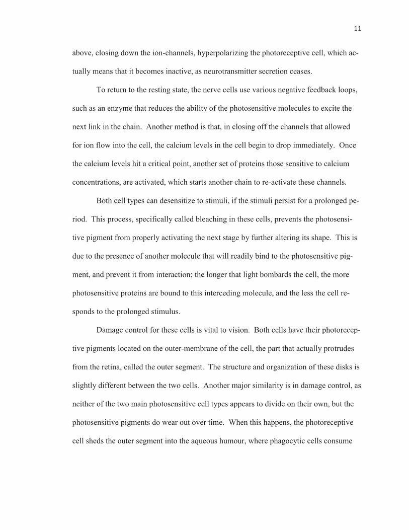
above, closing down the ion-channels, hyperpolarizing the photoreceptive cell, which ac-
tually means that it becomes inactive, as neurotransmitter secretion ceases.
To return to the resting state, the nerve cells use various negative feedback loops,
such as an enzyme that reduces the ability of the photosensitive molecules to excite the
next link in the chain. Another method is that, in closing off the channels that allowed
for ion flow into the cell, the calcium levels in the cell begin to drop immediately. Once
the calcium levels hit a critical point, another set of proteins those sensitive to calcium
concentrations, are activated, which starts another chain to re-activate these channels.
Both cell types can desensitize to stimuli, if the stimuli persist for a prolonged pe-
riod. This process, specifically called bleaching in these cells, prevents the photosensi-
tive pigment from properly activating the next stage by further altering its shape. This is
due to the presence of another molecule that will readily bind to the photosensitive pig-
ment, and prevent it from interaction; the longer that light bombards the cell, the more
photosensitive proteins are bound to this interceding molecule, and the less the cell re-
sponds to the prolonged stimulus.
Damage control for these cells is vital to vision. Both cells have their photorecep-
tive pigments located on the outer-membrane of the cell, the part that actually protrudes
from the retina, called the outer segment. The structure and organization of these disks is
slightly different between the two cells. Another major similarity is in damage control, as
neither of the two main photosensitive cell types appears to divide on their own, but the
photosensitive pigments do wear out over time. When this happens, the photoreceptive
cell sheds the outer segment into the aqueous humour, where phagocytic cells consume
12
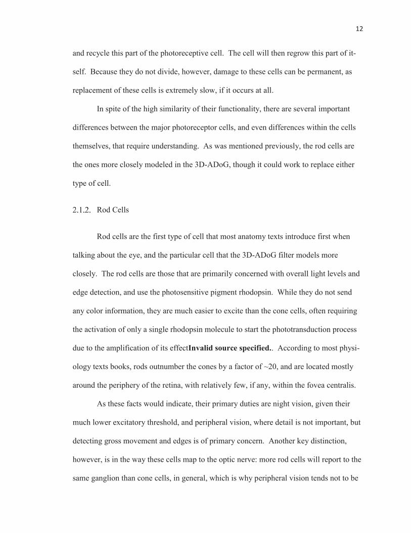
and recycle this part of the photoreceptive cell. The cell will then regrow this part of it-
self. Because they do not divide, however, damage to these cells can be permanent, as
replacement of these cells is extremely slow, if it occurs at all.
In spite of the high similarity of their functionality, there are several important
differences between the major photoreceptor cells, and even differences within the cells
themselves, that require understanding. As was mentioned previously, the rod cells are
the ones more closely modeled in the 3D-ADoG, though it could work to replace either
type of cell.
Rod Cells
Rod cells are the first type of cell that most anatomy texts introduce first when
talking about the eye, and the particular cell that the 3D-ADoG filter models more
closely. The rod cells are those that are primarily concerned with overall light levels and
edge detection, and use the photosensitive pigment rhodopsin. While they do not send
any color information, they are much easier to excite than the cone cells, often requiring
the activation of only a single rhodopsin molecule to start the phototransduction process
due to the amplification of its effectInvalid source specified.. According to most physi-
ology texts books, rods outnumber the cones by a factor of ~20, and are located mostly
around the periphery of the retina, with relatively few, if any, within the fovea centralis.
As these facts would indicate, their primary duties are night vision, given their
much lower excitatory threshold, and peripheral vision, where detail is not important, but
detecting gross movement and edges is of primary concern. Another key distinction,
however, is in the way these cells map to the optic nerve: more rod cells will report to the
same ganglion than cone cells, in general, which is why peripheral vision tends not to be
13
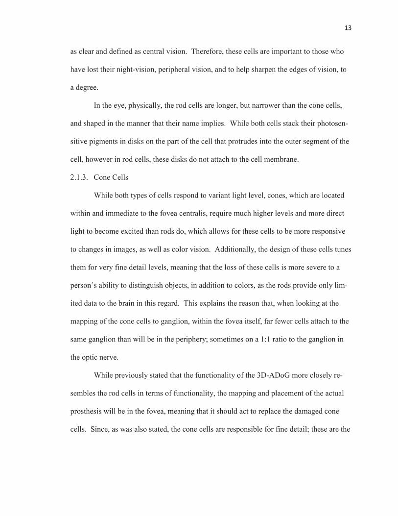
as clear and defined as central vision. Therefore, these cells are important to those who
have lost their night-vision, peripheral vision, and to help sharpen the edges of vision, to
a degree.
In the eye, physically, the rod cells are longer, but narrower than the cone cells,
and shaped in the manner that their name implies. While both cells stack their photosen-
sitive pigments in disks on the part of the cell that protrudes into the outer segment of the
cell, however in rod cells, these disks do not attach to the cell membrane.
Cone Cells
While both types of cells respond to variant light level, cones, which are located
within and immediate to the fovea centralis, require much higher levels and more direct
light to become excited than rods do, which allows for these cells to be more responsive
to changes in images, as well as color vision. Additionally, the design of these cells tunes
them for very fine detail levels, meaning that the loss of these cells is more severe to a
person’s ability to distinguish objects, in addition to colors, as the rods provide only lim-
ited data to the brain in this regard. This explains the reason that, when looking at the
mapping of the cone cells to ganglion, within the fovea itself, far fewer cells attach to the
same ganglion than will be in the periphery; sometimes on a 1:1 ratio to the ganglion in
the optic nerve.
While previously stated that the functionality of the 3D-ADoG more closely re-
sembles the rod cells in terms of functionality, the mapping and placement of the actual
prosthesis will be in the fovea, meaning that it should act to replace the damaged cone
cells. Since, as was also stated, the cone cells are responsible for fine detail; these are the
14
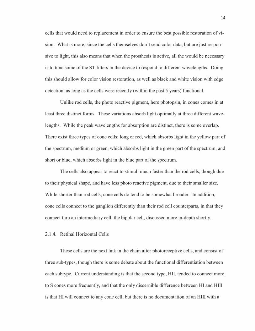
cells that would need to replacement in order to ensure the best possible restoration of vi-
sion. What is more, since the cells themselves don’t send color data, but are just respon-
sive to light, this also means that when the prosthesis is active, all the would be necessary
is to tune some of the ST filters in the device to respond to different wavelengths. Doing
this should allow for color vision restoration, as well as black and white vision with edge
detection, as long as the cells were recently (within the past 5 years) functional.
Unlike rod cells, the photo reactive pigment, here photopsin, in cones comes in at
least three distinct forms. These variations absorb light optimally at three different wave-
lengths. While the peak wavelengths for absorption are distinct, there is some overlap.
There exist three types of cone cells: long or red, which absorbs light in the yellow part of
the spectrum, medium or green, which absorbs light in the green part of the spectrum, and
short or blue, which absorbs light in the blue part of the spectrum.
The cells also appear to react to stimuli much faster than the rod cells, though due
to their physical shape, and have less photo reactive pigment, due to their smaller size.
While shorter than rod cells, cone cells do tend to be somewhat broader. In addition,
cone cells connect to the ganglion differently than their rod cell counterparts, in that they
connect thru an intermediary cell, the bipolar cell, discussed more in-depth shortly.
Retinal Horizontal Cells
These cells are the next link in the chain after photoreceptive cells, and consist of
three sub-types, though there is some debate about the functional differentiation between
each subtype. Current understanding is that the second type, HII, tended to connect more
to S cones more frequently, and that the only discernible difference between HI and HIII
is that HI will connect to any cone cell, but there is no documentation of an HIII with a
15
connection to an S cone. HII cells also are those which connect to rod cells, however, the
connection is so far removed from the more active center-portion of the cell that the con-
nection is nigh-trivial.
In terms of function, these cells are depolarized by the neurotransmitter gluta-
mate, which as was said previously is what the photoreceptive cells are passively releas-
ing when not stimulated. While depolarized, these cells release an inhibitory neurotrans-
mitter, GABA, to any photoreceptive cells in the immediate vicinity of the photoreceptive
cell that connects to, but which is not receiving stimulation: in other words, if the cell
connected to the horizontal cell is not firing, it will release GABA to ensure that no other
immediate cells are firing. When the photoreceptor cell fires, the decrease in glutamate
levels means that less GABA is produced, which means that it is now also more difficult
for the surrounding photoreceptors to fire.
In the 3D-ADoG by Karagoz et al [1], this is one of the sources of their described
ON/OFF, as the activation of a center cell deactivates a surround cell, unless the stimulus
to both is sufficient, and vice-versa. In the first stage of visual receptive field creation,
this cell is singularly the most responsible for the detection of edges.
Retinal Bipolar Cells
Similar to horizontal cells, these cells may exclusively connect rods, cones or hor-
izontal cells to the ganglion. Each cell can only accept one type of the above three as an
input, and output either directly to the ganglion, or to the amacrine cells (in the case that
the bipolar cell connects to rod cells, they will always connect to an amacrine AII cell).
Unlike any of the other nerve cells in this section, these cells do not use action potentials:
rather, they use graded potentials to pass on the information. In other words, they do not
16
fire in short, constant bursts, but rather alter their membrane potentials in a variant way,
for an indistinct amount of time. Similar to the photoreceptive cells, when the center bi-
polar cells receive stimuli from the cells prior to them in the chain, they actually enter a
state of inactivity. If the on-center cell receives sufficient stimulus, it hyperpolarizes and
becomes inactive, just like the photoreceptive cells; if it connects to a horizontal cell, the
off-center cells now become active, and the bipolar cell becomes inactive for the on-cen-
ter, and activates the off-center bipolar cells.
Unfortunately, it is at this point that the functions of the individual cells and lay-
ers in the chain of events for vision becomes significantly more hazy, as actual study in-
vivo is particularly difficult. Only the center bipolar cell mechanisms, like those previ-
ously discussed, are currently well understood, and generally accepted, in terms of how
they communicate, and how the information passes to the ganglia. As for the mecha-
nisms of the surround bipolar cells, while there are several theories about how this works,
there appears to be no definitive answer for what the mechanisms, molecular or biochem-
ically are.
These cells are found in the inner plexiform layer, which itself acts as a sort of
secondary excitatory/inhibitory response center, as well as a signal amplifier, before the
information is passed directly to the ganglion. In other words, the probably function, as
derived from what is known about on/off center cell interactions, is that it will further
amplify the edge detection from the horizontal cells.
Retinal Amacrine Cells
Very little seems to be in consensus about the function of these cells, other than
that they amplify whatever signals other cells transmit. What knowledge exists concerns
17
more regarding their structure: they have significantly vast dendritic trees. Like bipolar
cells, they exist in the inner layer of the retina, the inner plexiform layer.
Retinal Ganglion
These cells are located in the final layer of the retina, and transmit the information
from the previous layers directly to the brain, giving stimuli to several areas, most im-
portantly to our purpose being the visual cortex. Several facts are important about these
cells, and understanding of them is required for the functionality of the ST filter. First,
and most importantly is that the number of retinal ganglion cells is roughly 1% the num-
ber of photoreceptor cells, so multiple mapping is required. What is interesting about it
though is that the mapping is not uniform: the closer that the ganglion is to the fovea cen-
tralis, the fewer individual photoreceptor cells for which it has responsibility. The second
interesting thing is that even when at rest, it fires a constant pulse of action potentials.
When it is excited, then the frequency increases. This is what accounts for the brain de-
termining important information: if the ganglion is firing at a constant rate, no matter
what that rate may be, then the brain becomes desensitized to that stimulus, so the im-
portant information must always be causing a change in the rate of the ganglion firing in
order that the brain deem it of importance.
This might go so far as to explain the reason why desensitization is such a com-
mon problem in retinal prosthesis: from what has been read, it seems that these prosthesis
hyper-stimulate the ganglion with higher levels of electrical activity than biologically
normal [5], causing it to fire non-stop, and always fire at the same pulse for the same in-
put [6]. This is not how the ganglion is supposed to function, so the desensitization might
just be a function of the brain literally being bored with the input, or as a result of damage
18
from the increased electrical intensity [5].
These cells fall into categories based on where in the brain they deliver their in-
put, however, since this is unimportant to the prosthesis design, it in-depth discussion is
not necessary at this time. One fact of interest though was the discovery of a new type of
ganglion that is photoreceptive itself, and believed to be a part of regulation of the circa-
dian rhythm.
Simulating Cell Interactions
From the above, the order of operations becomes clearer, as does the mechanics
of how the device must work and the depth of how far the filter requires synthesis. Es-
sentially, the device needs to be able to simulate most of the interactions up to the optic
nerve itself. Essentially, light will strike the photoreceptive cells, which will then interact
with the first layer of the retina, which has excitatory cells, if it hits the connected photo-
receptors on-center, and inhibitory cells if it is hit off-center, as is the functional interac-
tion between the horizontal and bipolar cells, described above. This datum passes into a
second excitatory/inhibitory cell group, the amacrine cells, which, while understanding of
their function is by no means comprehensive, appear to act in the same manner, which is
to inhibit surround signals if on-center and excite surround while inhibiting the center if
the data are off-center. All of this information then electrochemically passes to a gan-
glion cell, that itself is part of the optic nerve.
The goal of the device is functionally to replace damaged retinal layers; therefore,
the device essentially needs to replace two layers of inhibitory/excitatory reactions. The
device proposed by Eckmiller appears to only functionally replace a single layer, which is
why, although we see some clarity, his image is not terribly fine-detailed. By contrast,
19
the double layering of Karagoz et al’s 3D-ADoG [1] becomes necessary to simulate the
two retinal layers: it is the only system seen so far that functionally simulates two layers.
The first layer functions as the excitatory/inhibitory reactios of the rod and cone cells,
and the second acts as the middle layer of the retina, with the bipolar and horizontal cells.
There exists at least one commonly observed issue, however, and one that could
be difficult to overcome: in cases where vision has been lost for an extended period, the
body tends to shut down to stimulus from the optic nerve for those damaged cells. If this
is the case, then no prosthesis currently available will be able to get these nerve cells to
respond again. In addition, because of the designs of many prostheses, the brain tends to
stop responding to stimuli from the prosthesis after a relatively short period.
A key metric for the success of this is the timing: the brain receives the data and
interprets the image at a rate of roughly 30Hz; therefore, this program needs to run at a
speed of more than 33ms, in order for the image to be as smooth as possible. There is
something of a range, as this is the upper limit to the speeds of the eye, and realistically, a
speed of ~20Hz would be acceptable.
The majority of how the biological function is simulated is discussed in the sec-
ond and third sections of chapter 3, the next chapter.
20
CHAPTER 3: ST FILTERS
The spatio-temporal (ST) filter is the device that simulates the cellular functions
described above. Essentially, the device will function to interact directly with the gan-
glion thru electrical impulse, using methods described below, to simulate the functional-
ity of the damaged layers of the retina. The number of filters that will be required will be
discussed in greater detail below, however, suffice to say that the number of filters cold
in theory be equal to the number of photoreceptor cells, depending on how detailed the
image should be. Since, for this particular design, the assumption then was that this de-
vice would be near the fovea centralis; that it functions as though there is a 1:1 ratio be-
tween the number of ST filters, and the number of photoreceptive cells.
In his paper, Eckmiller discusses the fact that his filters are tunable. This relates
to some of the specifics of the design that will be discussed in further detail below, how-
ever, the fact is that there are numerous ways to alter the output of the image. Some of
these have to do with the clarity of the image, others with the way that overlap is simu-
lated, etc. While none of these particular methods for tuning are able to be tuned on the
fly in the prototype, to be able to do so is very obvious, in terms of where these tunings
should apply, and may be used in future applications.
Gaussian Filters
The Gaussian filters forms the backbone of the entire process for the visual pros-
thesis designed here: essentially, the value of any given pixel changes based on the dis-
tance between that pixel and a defined center value. In practice, this is similar to the way
that the cells embedded in the retina will inhibit or amplify the signal received from the
21
photoreceptive cells. In this design, the stronger the stimulus is near the center, the more
focused it will be at the center, and the more diffused it is, the more evenly spread this ef-
fect will be across the entirety of the filter.
The formula for a single Gaussian filter is as follows, where A is a given ampli-
tude value, σ is the standard deviation for the area’s portions, and the variables x and y
represent the difference along their respective axis (x or y) from the center coordinate [1]:
This equation calculates both the center and the surround values for any given re-
gion. The major change between the center and the surround comes from the A values
for the respective region: the surround has a smaller amplitude value, as was taken di-
rectly from Karagoz et al [1], due to the fact that these should have a lesser impact on the
output of the image as compared to the center. The surround portion is representative of
the off-center cells, while the center is representative of the on-center cells. Since the on-
center strike is the more important of the two, the weight of it, represented by the ampli-
tude is the more important, and therefore more heavily weighed of the two.
As has been stated, the design uses this formula twice: once for the center, once
for the surround parts of the given image or area of the image. What happens next is
finding the difference between the two to simulate the on and off-center strikes. If the
strike is stronger on-center, simulating if the strongest light is hitting the central photore-
ceptive cell, then the output value will be greater than zero, and sends a signal to the next
level, indicating that the output should produce an image. If the surround is stronger,
however, then the output should be zero or less, which inhibit the response chain de-
22
scribed in the previous chapter. To find this result, a difference of the center and sur-
round Gaussians (difference of Gaussian or DoG) is used [1]:
This is the actual equation that constitutes an ST filter, and constitutes the bulk of
the work that each section of the program will do. This indirectly simulates the work of
the photoreceptive cells themselves, and more directly the horizontal and bipolar cells in
the next retinal layer. Discussion on this topic continues, in further depth, in the imple-
mentation chapter.
Gaussian Radius
An important aspect discovered during implementation was that the system seems
to work best when fully simulating that the area covered by each photoreceptive cell is
finite and smaller than the whole image in size. That is, if each filter is responsible not
for the image as a whole, but only a selection. While this too will be discussed more in-
depth in the implementation, the important piece is that without this, because of the na-
ture of the second part of the equation, , the larger the area that is covered, the
more rapidly, the entire equation resolves to zero, meaning that no visual data is inter-
preted.
The addition of the radius function has a two-fold effect because of this. First, it
simulates the fact that no cells are going to have full visual field access; they will only be
perceptive of a small portion of the area. Second, it makes sure that there is viable output
from the DoG equation, as both of the equations would otherwise resolve to zero, mean-
ing no output, no matter how strong the signal, or else an output that is a single white
23
pixel surrounded by black, or a single black pixel surrounded by white. Eckmiller dis-
cussed this in his paper, and the implication was that these would be the desired results
under ideal circumstances. However, this is not what is ideal for image reconstruction.
To ensure that this did not become the standard, it is simple enough to place a limit on the
function, so that it only covers enough area to prevent that part of the equation from aver-
aging out to zero.
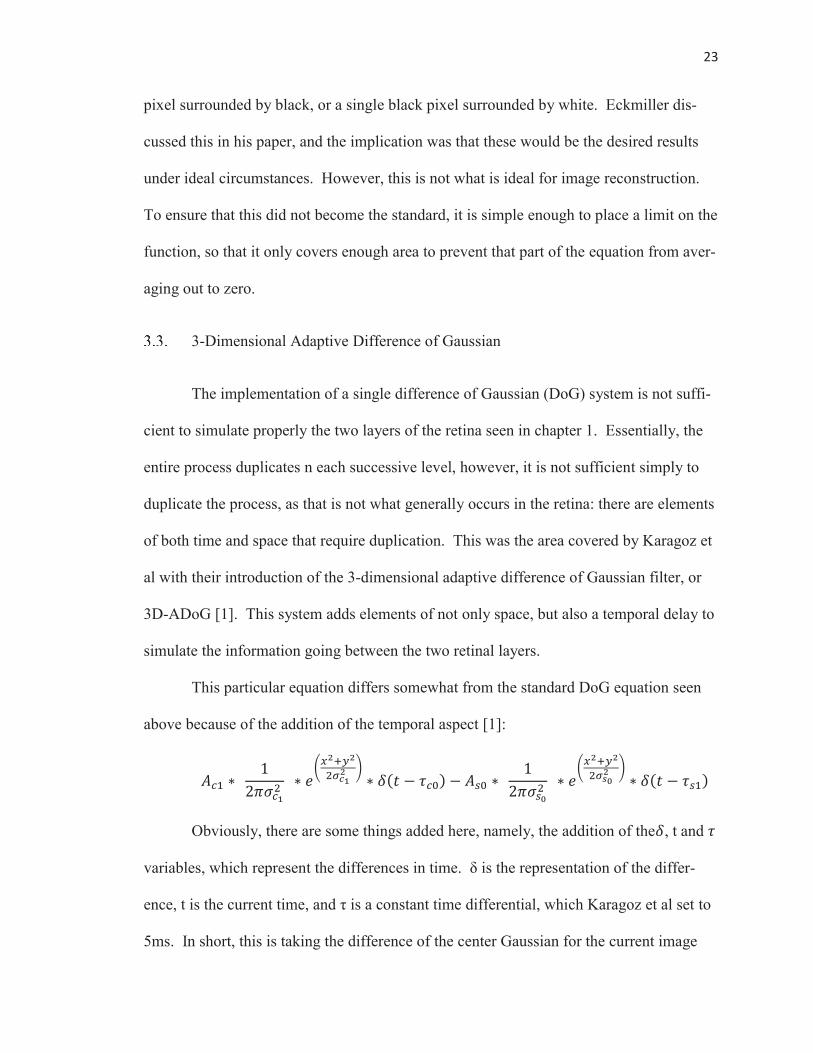
3-Dimensional Adaptive Difference of Gaussian
The implementation of a single difference of Gaussian (DoG) system is not suffi-
cient to simulate properly the two layers of the retina seen in chapter 1. Essentially, the
entire process duplicates n each successive level, however, it is not sufficient simply to
duplicate the process, as that is not what generally occurs in the retina: there are elements
of both time and space that require duplication. This was the area covered by Karagoz et
al with their introduction of the 3-dimensional adaptive difference of Gaussian filter, or
3D-ADoG [1]. This system adds elements of not only space, but also a temporal delay to
simulate the information going between the two retinal layers.
This particular equation differs somewhat from the standard DoG equation seen
above because of the addition of the temporal aspect [1]:
Obviously, there are some things added here, namely, the addition of the , t and
variables, which represent the differences in time. δ is the representation of the differ-
ence, t is the current time, and τ is a constant time differential, which Karagoz et al set to
5ms. In short, this is taking the difference of the center Gaussian for the current image
24
(c1), and subtracting it from the surround value of the previous image (s0). This occurs in
order to simulate the image’s path thru the retina, and works under the assumption that it
takes longer for a surround reaction to activate than direct, on-center action. This is
somewhat supported in the first layer of the retina, however, as was stated previously, it
is not known if it occurs in the second layer. The main thing here, which separates it, is
the fact that it takes multiple images into account, rather than just a single, static image,
which is closer to how this would function in the eye, which will be constantly receiving
input.
The fact that it is taking the surround as the slower of the two input is of interest.
In the Karagoz et al paper, the τs is always set to 5ms less than the τc in order to represent
this. While it is not made clear in their paper, that is what was the clue that the center and
the surround come from two different images, rather than simply trying to make the sur-
round simply more powerful than the center image, to try and balance it out. This was
initially the point of some contention, as with a static image, this equation still works, but
makes much more sense given our particular implementation of the paper, which is the
subject of a later portion of this thesis. In short, as was said earlier, the basis for this was
the idea that information constantly bombards the eye, combined with the fact that the
signals for an off-center signal to the brain take longer than those for on-center would.
This biologically also make some sense, as it would take more stimulus to get these cells
to fire if they are not in the central focus of the light, especially in the area of the retina
that is the focus of this process.
These reasons, the multiple image applicability, the addition of a temporal ele-
ment, and the fact that it more closely resembles the biological function of the eye, led to
25
the choice of this particular version of the DoG for the prosthesis. In addition, their par-
ticular implementation assumes damage to both layers of the retina, and so would be able
to function regardless of how much damage, so long as the optic nerve and the individual
ganglion are still functional. The only issue with this assumption is the previously men-
tioned fact that the body tends to desensitize to stimuli, especially if the damage has been
persistent, or the individual has not had “normal” vision for some time.
The final part of the 3D-ADoG is the noisy-leak, integrate and fire (NLIF) sec-
tion, which is what determines if the ganglion should receive sufficient electrical stimulus
to fire. This piece is essentially the go-between for the amacrine and retinal ganglion
cells, and assumes that the ganglion themselves are still active. It uses a unique equation
set, one for if the neuron will fire, and one if it does not, based on the voltage threshold.
The more interesting equation is what happens if it does not fire, and it is as follows [1]
[7]:
Essentially, at time tn, voltage V is equal to the voltage from time tn-1, plus the in-
tegral of the current ( ) is this after it has been integrated) and a noise constant
that they added to simulate the noise that naturally occurs in optic nerves. The result of
this is that the previous state of the nerve has a direct influence on the current state. This
essentially simulates the previously mentioned state of the retinal bipolar cells: that of
graded potential. If the cell does reach a certain level, however, it acts like any other
nerve cell and will immediately reset to that cell's resting state. In a pure form of the im-
plementation as described by Karagoz, there would also exist an absolute refractory pe-
26
riod, whereby no matter what, the cell cannot fire again. This is also in line with the biol-
ogy. The equation for if the observed voltage is greater than the spike threshold follows
[1]:
To sum this equation up, if the voltage at time t is sufficient to fire an action po-
tential, then the voltage automatically resets to the resting potential, and a spike is then
generated.
Basics Of This Implementation
This will be touched more in depth in the next chapter; however, some elements
are necessary to clarify now. First, this implementation of the 3D-ADoG is the particular
version of DoG that used. Second, its use assumes that there will be images coming in at
a constant rate from a specific source. This is to ensure, as seen in Karagoz et al, that the
successful implementation of both retinal layers. This implementation does not include
the NLIF itself, however, as that part very quickly became too difficult to implement in
any meaningful function in time for the defense of this thesis.
It is now possible to lay out the basic steps of how the filter functions here with-
out going into the specifics of this implementation. The first step is the normalization of
the image data, which keeps any spikes to within a constant range. This normalized im-
age then runs thru the first stage of the 3D-ADoG, which is an ST-filter. This process is
to take the formula and use the normalized image data to create, essentially, a new image
data file that is a Gaussian distortion of the normalized data, mimicking the output from
the outer retinal layer. This new file is then normalized and passed thru a second filter
27
bank, using the output of the first filter bank in place of the normalized data from the first
run-thru. This is the point at which the implementation described here will stop, how-
ever, to truly simulate the eye down to the ganglion level, a third step, the NLIF, is used
in the manner described above.
Once this file is received, it is decoded and reconstructed into an output image.
This output image is not what the user would see, but is rather a decoding of the data that
would go into the NLIF. Areas that are brighter are those that would most likely produce
a positive reaction from the NLIF, resulting in it firing. Those areas that are darker
would result in the NLIF not firing, and would be black. The NLIF would be tuned to a
threshold, so this could be adjusted, just like in Eckmiller et al. This tuning was im-
portant to Eckmiller, but this implementation allows for very easy addition of an addi-
tional tuning parameter that Eckmiller did not allow for: the tuning of individual image
sections. Because of the modularity of this implementation, it is possible to specify
which areas of the image will go to which filters, and what the intensity of the section
should be relative to the other sections. This would allow for greater control over the
damaged areas of the retinal cells than was seen in Karagoz or Eckmiller.
28
CHAPTER 4: PIPELINING
As was stated in the introduction, one of the important aspects of this thesis is the
potential improvements to speeding up the current processes, so that the other aspects
may fall into place, and with the correct timings. Pipelining was determined early on to
be one of the easiest ways to do this, as given the two-layer model, it fit perfectly into the
paradigm.
Basics Of Pipelining
Pipelining is a relatively simple process, and one with a well understood imple-
mentation within the computer science community, as it is one of the older methods of
speeding a process up. In order for pipelining to function, the output of the first part of
an operation or function must be the input of the second part of that operation or function.
Additionally, the output of the first part of this operation or function must not affect or be
required by a new instance of the function or operation. In other words, that each opera-
tion or function is discrete, but that the outputs of the first stage can function as inputs for
the next stage, which is also its own discrete function. The end goal is that the operations
at any given point, and which exist in the pipeline all execute at the same time, or roughly
thereabouts. Therefore, one part from the first stage and one part from the second stage
occur in the same clock cycle, instead of performing all of the first stage, then all of the
second stage, then the next operation’s first stage again, and so on.
It is of great importance to understand, however, that the initial image output will
take the same amount of time, regardless of whether or not pipelining exists in the sys-
tem. The reason that this becomes important is two-fold. First, it is demonstrative that it

29
does not speed up the process of each image output, but rather the bandwidth of the sys-
tem as a whole. This allows the ST filter system for this project to work on multiple im-
ages at different levels simultaneously. Second, it gives a benchmark to measure whether
the system produces the images with the correct timing. Therefore, it is a method of
speeding up the project that requires no hardware dependence, unlike the addition of
multi-threading, or requiring a multi-core environment. It is also much easier to imple-
ment in any software or hardware architecture than the above two other methods. As a
matter of best practice, making no assumptions about either the hardware or general envi-
ronment in which the prosthesis will eventually exist remains highly important, and so
the goal becomes making this as universal as possible.
For these reasons, pipelining became the primary focus of the speedups in this
project, rather than multi-threading, or multicore dependency. Though it would be a sim-
ple matter to implement, especially regarding miniaturization, to assume and to create a
device containing at least 2 processing units, this assumption violates best practice, and
the attempts made at multi-threading in Java produced results that, while very fast, were
extremely unreliable. This is one of the subjects of chapter 6.
Implementation In This Project
This particular project follows a very basic pipeline procedure, however, despite
this simplicity; its importance cannot be overstated: the pipeline was the most significant
addition to the design. As stated previously, the entire system requires precise timing.
The problems that were encountered show that the system needs a way to speed itself up,
and that while multi-threading does sufficiently speed the system up, it is not reliable
30
enough to produce stable images at the rate needed. However, the images need pro-
cessing at very specific intervals, and within very specific periods for the entire process
to function. The multi-threading within the image processing obviously doesn’t work,
however, it might be possible instead to multi-thread each image as it comes in, pro-
cessing multiple images at once. While in their paper, Karagoz et al emphasize a timing
of only 5ms between each image, this does not quite work for this particular design.
However, it does allow for a diagram of the pipeline system that is easier to read and un-
derstand. In reality, the time between each stem in this system would ideally come out to
roughly 30ms, rather than the proposed 5ms, but this is in order to meet the goal of ~30
frames per second. As was discussed in section 1, while this is the maximal number of
times that the image on the eye would be refreshed in-vivo, it is not the normal operating
number of frames per-second that they eye would normally see; that number is closer to
20-25 frames per second. Any more speed than this would be wasteful.
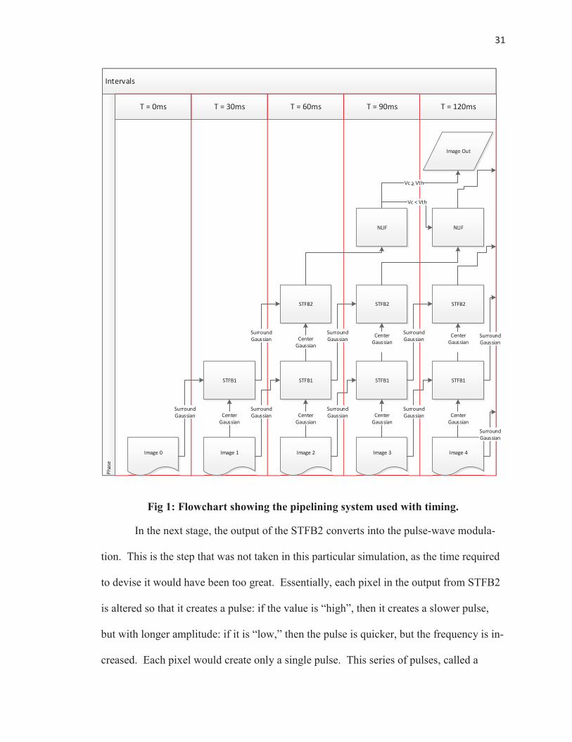
To explain the following diagram, the bottom row is the image series coming in
from the source. The surround matrix calculated from initial processing of the image at
stage n-1 then combines with the center matrix from the image at stage n in the first filter
bank of the STFB. This STFB outputs what essentially amounts to another image, with a
center and surround matrix of its own. The surround part of this matrix, the output from
the STFB run at time n, becomes the surround matrix in another STFB filter bank, with
the center matrix from the STFB run at time n+1. The output from this STFB is a combi-
nation of the outputs from the lower-level STFBs and is a Gaussian distortion of a Gauss-
ian distortion. This means that it does function in a manner very similar to how the hu-
man eye is supposed to function, in accordance with current understanding.
31
Intervals
T = 0ms T = 30ms T = 60ms T = 90ms T = 120msPh
ase
Image 0 Image 1 Image 2 Image 3 Image 4
STFB1 STFB1 STFB1 STFB1
SurroundGaussian Center
GaussianCenter
Gaussian
SurroundGaussian
SurroundGaussian Center
Gaussian
SurroundGaussian Center
Gaussian
SurroundGaussian
STFB2
SurroundGaussian
STFB2
SurroundGaussian
STFB2
SurroundGaussian
SurroundGaussian
CenterGaussian
CenterGaussian
CenterGaussian
NLIF NLIF
Image Out
Vc > Vth
Vc < Vth
Fig 1: Flowchart showing the pipelining system used with timing.
In the next stage, the output of the STFB2 converts into the pulse-wave modula-
tion. This is the step that was not taken in this particular simulation, as the time required
to devise it would have been too great. Essentially, each pixel in the output from STFB2
is altered so that it creates a pulse: if the value is “high”, then it creates a slower pulse,
but with longer amplitude: if it is “low,” then the pulse is quicker, but the frequency is in-
creased. Each pixel would create only a single pulse. This series of pulses, called a
32
pulse-wave modulation, is the backbone of the creation of what is referred to as the spike
train in most papers regarding visual prosthesis, and it is the key to converting the digital
signal into one that can be understood by the ganglion cells. This pulse wave modulation
then feeds into the NLIF, which itself acts as an artificial neuron [4]: if the pulse’s ampli-
tude matches the threshold value, then it generates a spike, otherwise, the next spike uses
the output of the current spike for its own spike amplitude determination [7]. This creates
a visible chain of spikes, and recreating the image from this chain of spikes is the key to
recreating vision in the human eye using a digital prosthesis.
The pipeline system is not without its own drawbacks. First, it does take four cy-
cles to get thru all four stages of the ADoG. Second, to function ideally, it would require
that each of these stages runs as a separate thread, given all of the positives and negative
effects that multi-threading had in the past. However, this system exists in the current
model of this project’s STFB, albeit in modified form, in the final version of the project.
Initial Attempts
The initial attempts at pipelining the system were not terribly successful, as the
entire program initially ran as a single class, without any branching allowed. This pre-
vented the program from ever having two distinct objects, like what the figure above
shows. Instead, what resulted was a single object, where the program applied the mathe-
matical operations to both images as though they were a continuous input stream of data,
essentially as though they feed in like a continuous fax machine. What this resulted in
was an image with a very definitive center and surround output, instead of what the de-
sired result should be: a smooth image.
The solution to this was very simply: break the image apart into its own separate
33
object, and perform the tasks in the same manner depicted in the diagram above (which
did not exist in written form at this point). By doing this, each image object performed
all of the functions that would be required of it in the first stage of the pipeline, and then
the individual arrays created and manipulated with the output of the next image, undergo-
ing the same process, in the second stage of the pipeline. By doing this, run time was re-
duced, since the images arrived, essentially, pre-rendered, and all that is needed is a sim-
ple subtraction operation on the two, in accordance with the formula presented earlier.
This output is then subject to the same process, but merged now with the new input im-
age’s properties. The result is a significant reduction in the running time of the whole
process, since this creates each image object with these required properties, rather than
having to go thru one at a time, individually.
This also lends itself naturally to multi-threading the operation, as the creation of
each object runs independently of the creation of any other object. Naturally, this would
also serve to further reduce the running time and bring it within the required parameters.
Resulting Attempts
As was stated above, the breaking down of images into their own discreet objects
is what eventually led to the success of the pipeline implementation in this architecture.
In addition, the speedup that it produced was almost double that of trying to run each
stage of the pipeline consecutively. Running concurrently, with some multi-threading,
created increases in speeds that approached the threshold required, despite a much higher
resolution than the image used in the final prosthesis, though without the desired reliabil-
ity or stability. The promise this holds is astounding, as minor improvements in hardware

34
could mean significant increases in the resolution used in these prosthesis, once the hard-
ware is able to handle them.
While the timing is the discussion of a later chapter, the speedup potential intro-
duced is still fairly phenomenal: even the most complex versions now take less than a
third of the original run-times for the first prototypes, with most coming in at under a sec-
ond, all while performing far more work. In short, this particular breakthrough, in con-
junction with the radius function that is the subject of the chapter on the development arc,
constitutes a major component in the functionality and feasibility of this project.
35
CHAPTER 5: MAPPINGS
As stated in the introduction, one of the goals of this project was to ensure that the
programs more accurately reflected human visual processes. The current paradigm only
has a 1-to-1 ratio when it comes to mapping, so one of the project’s sub-tasks was to see
if this was indeed the most efficient means to perform these processes. Unfortunately,
this does not accurately reflect the real function of the human eye, as the retinal cells do
not exist independent of each other. Therefore, two important reasons were found to ex-
amine the different ways to map the images and ST filters.
Mapping Types
The first of these challenges addressed was how to map the ST filters to the im-
ages themselves. Indeed, reading the papers on the subject, it was not clear if they sec-
tionalized the images, ran each image thru a series of filters, or any such useful infor-
mation; all information given from Eckmiller et al, for example, was the number of fil-
ters, the number of tuneable parameters and the size of the image. The clue came from
Karagoz et al when they proposed their dual-layer 3D-ADoG: they ran their image thru
two-layers of ST filters, and claimed superiority over the older, single-layer. From the
information given, it was relatively easy to infer that the previous models had all used a
single-layer of ST filters spread out over the image.
The next question came down to how to sectionalize the image. In the earliest
versions of the development of this project, the image was not sectionalized at all, and
this resulted in extremely slow run times, as each pixel was compared to every other
pixel: over 260,000 comparisons per run-thru. This is why the addition of the radius
36
function became so vital to the process: it dramatically reduced the number of calcula-
tions required. While it would be possible to design a system that uses these filters in any
manner of shapes, for simplicity, it was decided to keep them all uniform in size: it saves
on trying to cut the image out into certain shapes, it is easier to develop and maintain, and
it is more universal to distortion and edge detection. To do this, a mapping scheme was
required, and four separate types of mapping required consideration.
1-To-1 Mapping
This is the simplest form of mapping implemented in a design such as this project
and it is the version that, so far, has proven to be the most effective, in terms of timing.
In this type of mapping, as the image is broken down, each section of the image used in
one, and only one ST filter. The output, therefore, is also mapped to the same area: so
that if the image is broken into 15x15 pixel squares, each ST filter will output a 15x15
pixel square
Though not 100% necessary, for all of the versions of the ST filter that were explored
here, this was used in the implementation to both avoid confusion and speed up the image
rebuilding process, as well as to ensure proper image reconstruction when the filter had
finished running. As stated, since this is generally the simplest form of mapping, the ini-
tial hypothesis was that this should be the fastest, and that will be covered in chapter 5.
All versions of the program using the radius without overlap design for the ST filters in
this project use this mapping type and the results in terms of the images are across the
board in terms of clarity, though generally among the best. All of these instances use the
mean values from the output in the reconstruction of the image post-ST filtering.
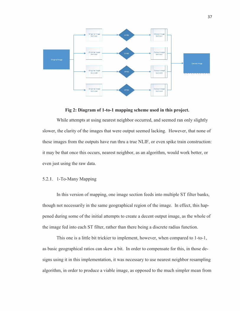
37
Fig 2: Diagram of 1-to-1 mapping scheme used in this project.
While attempts at using nearest neighbor occurred, and seemed ran only slightly
slower, the clarity of the images that were output seemed lacking. However, that none of
these images from the outputs have run thru a true NLIF, or even spike train construction:
it may be that once this occurs, nearest neighbor, as an algorithm, would work better, or
even just using the raw data.
1-To-Many Mapping
In this version of mapping, one image section feeds into multiple ST filter banks,
though not necessarily in the same geographical region of the image. In effect, this hap-
pened during some of the initial attempts to create a decent output image, as the whole of
the image fed into each ST filter, rather than there being a discrete radius function.
This one is a little bit trickier to implement, however, when compared to 1-to-1,
as basic geographical ratios can skew a bit. In order to compensate for this, in those de-
signs using it in this implementation, it was necessary to use nearest neighbor resampling
algorithm, in order to produce a viable image, as opposed to the much simpler mean from
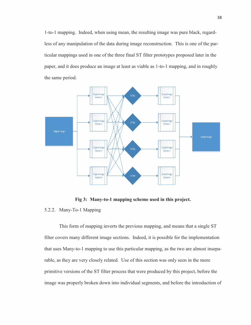
38
1-to-1 mapping. Indeed, when using mean, the resulting image was pure black, regard-
less of any manipulation of the data during image reconstruction. This is one of the par-
ticular mappings used in one of the three final ST filter prototypes proposed later in the
paper, and it does produce an image at least as viable as 1-to-1 mapping, and in roughly
the same period.
Fig 3: Many-to-1 mapping scheme used in this project.
Many-To-1 Mapping
This form of mapping inverts the previous mapping, and means that a single ST
filter covers many different image sections. Indeed, it is possible for the implementation
that uses Many-to-1 mapping to use this particular mapping, as the two are almost insepa-
rable, as they are very closely related. Use of this section was only seen in the more
primitive versions of the ST filter process that were produced by this project, before the
image was properly broken down into individual segments, and before the introduction of
39
the radius function, which essentially switch this to 1-to-1. The reasons for this will be
included and discussed more in the next chapter, where timings discussions are more the
focus.
In terms of spike train generation, either mean or nearest neighbor could work,
though conjecture would put nearest neighbor as the more likely candidate. The reason
for this is its similarity to 1-to-Many mapping, which produced results only with nearest
neighbor, and did not produce a viable image when using the mean. However, since no
viable image was ever the outcomes using this method once the implementation of image
section compartmentalization took effect, it is not easy to tell if this would actually be the
case.
Many-To-Many Mapping
As was stated before, this is the version that is closest in function to the human
eye: light does not hit the photoreceptive cells in discrete, packaged areas, and the brain
interprets based on changes between each photoreceptive cell group. Therefore, this
mapping should produce the most coherent images when it transfers into a spike-train.
As to how the image translation occurs, the clearest images that this particular mapping
produced were those that used mean to determine the final output image. As to the close-
ness of how this works in the eye, it is important to note that the ganglion receives input
from multiple sources, each of which do have an effect on the neighboring cell groups.
Therefore, more experimentation would have to occur to see which produces a better
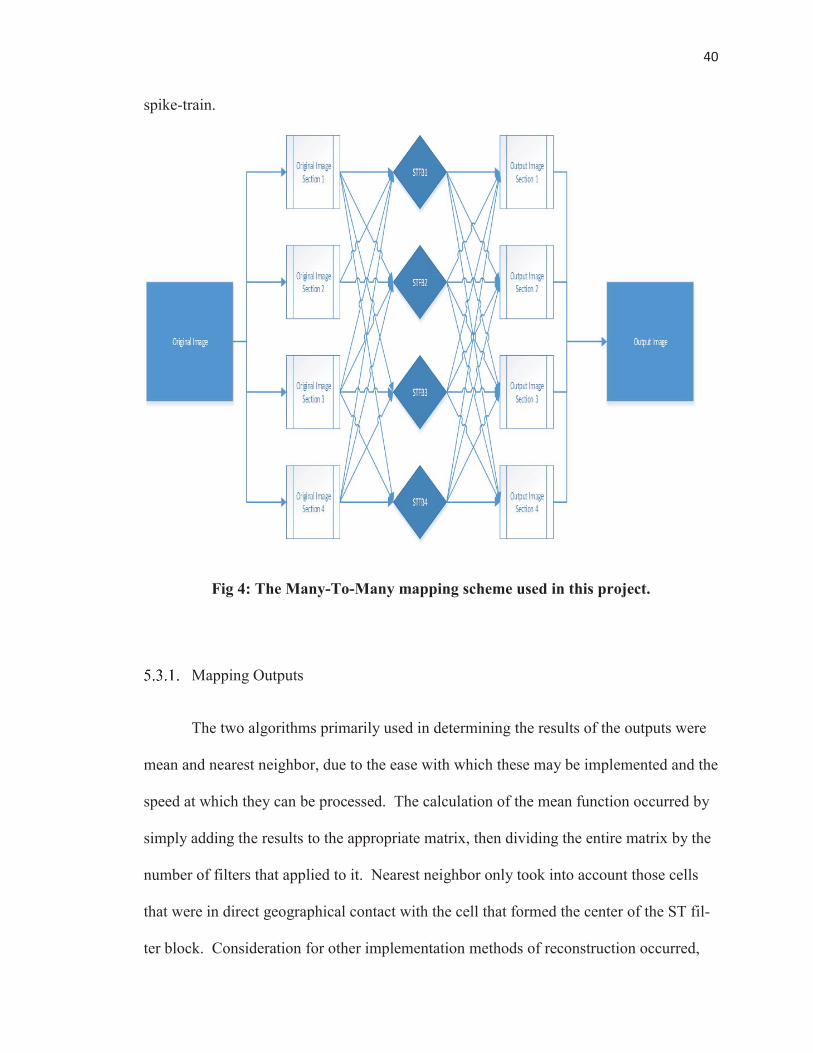
40
spike-train.
Fig 4: The Many-To-Many mapping scheme used in this project.
Mapping Outputs
The two algorithms primarily used in determining the results of the outputs were
mean and nearest neighbor, due to the ease with which these may be implemented and the
speed at which they can be processed. The calculation of the mean function occurred by
simply adding the results to the appropriate matrix, then dividing the entire matrix by the
number of filters that applied to it. Nearest neighbor only took into account those cells
that were in direct geographical contact with the cell that formed the center of the ST fil-
ter block. Consideration for other implementation methods of reconstruction occurred,

41
but there was insufficient time to implement them, so these two received the most atten-
tion.
It is of note that none of the papers discusses this particular aspect of how to
check on the program: all of this had to come from scratch. The papers are all more con-
cerned with the output of the NLIF; however, this step is vital, as it allows the user to en-
sure that the image distortion occurs in a manner that they wish to use. To focus solely
on the NLIF, which itself is substituting for the optic nerve will be the next step, and it is
debatable as to whether this part will be of any use to that portion of the project or not:
whether the data should be normalized or raw coming out of the ST filter.
Mappings Implementations
The project used various mappings at different points throughout the project, but
some were of greater use. By far, the most used were the 1-to-1 mapping because of its
relative ease, and the Many-to-Many mapping because of its effectiveness. To actually
implement the other two, 1-to-Many and Many-to-1, in their purest forms becomes ex-
tremely difficult in this particular situation, especially when attempting to reconstruct, in
software, something that actually functions like the human eye, and which does not turn
into either a 1-to-1 or Many-to-Many mapping.
For example, while Many-to-1 exists in one of the final three versions of the pro-
gram put forward, the difference between it and the Many-to-Many version is a very
slight alteration. To explain, the addition of a finite radius to the function that only al-
lows for a partial use of each image section surrounding the central body, so the whole of
the 1 is never used twice, at which point it would become Many-to-Many, instead. Simi-
larly, the attempts to create a true 1-to-Many mapping scheme kept resulting in either the
42
system locking up, or else the same effect as Many-to-Many, as the borders between the
image sections are extremely well defined.
This results from the fact that in order to produce any sort of image at all, using the
discrete section method, it becomes necessary to severely limit the radius of these sec-
tions, as otherwise the values produced by the ST filters very quickly rounds to 0. If this
were not the case, and the borders of the sections were more free, this would be much
easier to implement, and indeed, with future work, might be the way to go. For now,
however, because the finite sections model was used in order to speed up the process,
these two particular forms of mapping have limited, and somewhat subjective use in this
project.
Of the final three versions of the code, two of them only have one implementation:
1-to-1 and Many-to-1. For 1-to-1, this is because the code does not require any sort of
averaging out in order to reconstruct the image, as each section remains unaffected by
those image sections around it, so any image manipulation is not required, and would
only be necessary to sharpen, brighten or dim the image. For the Many-to-1, a mean
function does not work, and never produced a viable image, because while portions of
each image section are used at several points, the whole section itself is not used, so it
would require averaging out each pixel based on the number filters that particular pixel is
fed thru. This is both time consuming, and unnecessary to produce a viable image, as
will be seen in chapter 6. While an initial attempt at a version that used the mean existed,
it was discarded very quickly, and the code no longer exists due to a crash. It never pro-
duced anything other than a pure-black or gray image, no matter what parameters used.
The final version of the Many-to-Many mapping, however, is different, in that two
43
versions of the code do exist: one using mean, the other using nearest neighbor. While
one does arguably produce a much higher quality image reconstruction, this sis somewhat
subjective, and left up to the future designers. The timing differences between the mod-
els used is the subject discussed in the next chapter.

44
CHAPTER 6: TIMING AND MAPPING
INTERACTIONS
Again, in order to more accurately recreate the human visual process, both the
timing and the mappings must be correct. The average speed for the human eye would be
processing images at roughly 30 images per second, though the actual range is more var-
ied. While this number was not achieved, another, more important piece of information
was: namely, the exact trade-off for how close the overlap of the cells in the eye can be
recreated, and how much extra time each of these particular types of mapping require.
A key point to stress is that the times that are listed should not be considered as
absolutes. Instead, they should be used as a measurement against each other, given that
the device used to run them was neither designed for the task, nor was able to run them
exclusively. Therefore, if a runtime for one model is 15ms, and another model is 30ms, it
is not that they will always run this fast on given hardware, but rather that the runtime of
the second model is roughly twice that of the first. This is why the averages were used,
as well, since the run times varied wildly depending on what was also running on the ma-
chine at the time.
Timing For Original Designs
The speeds showed derive from the average run times seen running the program
on a personal computer, which is admittedly much more powerful than the device in
question will be, at least with current hardware limitation. Since this was all written in
Java, and is machine independent, the times should at least be similar, so what will be
represented are the ratios of the times required for each run in comparison of the original
45
prototype, as well as the actual averaged run times themselves. All times shown are in
milliseconds.
Original Prototype
The run-time for the original prototype was 11,955, and since this is used as the
base, it has the ratio number of 1. This was incredibly slow mostly because it required
treating every pixel, in essence as its own filter in order to recreate the image, but the out-
put, as was seen, is still not terribly clear, and does have the photonegative effect, so the
trade-off is not exceptionally worthwhile. In addition, unlike the latter attempts, this one
did not break the image up into two distinct runs thru the equation, but rather consisted of
only a single run thru the ST filter process: so it uses only one bank of filters, and runs at
over 11 seconds. It is also only capable of using a single image, and cannot merge the
images as they come in, as the final version will.
This model however, did serve as the basis for all of the models to follow it, and
so it does deserve some respect, as even the current models use the same system to break
down the image. The slowness results from the naïve manner in which it breaks the im-
age down, and reassembles it, all without pipelining or multi-threading. The latter mod-
els, while they do use this basic setup, do so in a much more streamlined manner.
One thing to note about the timing is that it is actually from a slightly modified
version of the original version: one that uses a more refined version of who to determine
the required number of filters. While it does do a comparison of every pixel to every
other pixel, hence the extremely slow speed, but there are a finite number of filters that
are in use; 256 by default.
46
The Addition Of The Finite Radius
The addition of the radius was the single greatest reduction in run time over the
previous version: it has an average run time of 541ms, giving it a ratio of 0.04525. This
came the closest of the current models to meeting the requested speed of 33ms, or a ratio
of 0.00279. More about the specifics of the radius function is the discussion of the next
chapter; however, the reason for the improvement was that it simply reduced the number
of pixels that were involved in each comparison. It also ensured that each pixel is dis-
crete: not used as an element to every other pixel, but only to those within its own cluster.
It still uses the same number of filters as the prototype, as it comes from exactly the same
template.
This means that many of the reasons as to why it runs as it does are the same: the
same naïve rebuilding of the image form the direct and unmodified pixel values, a similar
manner of how it breaks apart the image, etcetera. However, there exists another key dif-
ference: each image block is essentially broken into its own array, totaling 256 small ar-
rays that are used in the ST filter block. Therefore, the overall speed, as discussed in the
next chapter, is not quite using the same metrics, and it has its own reasons for speed re-
duction.
The Addition Of The Overlap With The Radius
As can be expected, the addition of more pixels to the comparisons increased the
run-time of the entire program by a slight margin, though it also did increase the overall
clarity of the image. The new run time, with a margin of 15-pixels of overlap was 837, a
ratio of 0.07001 to the original, and 1.54713 to the program without the overlap. In other
47
words, adding 15 pixels, which at the time, the overall radius was 16 pixels when there
was no overlap, increased the run-time by only 155%: so a near double increase in the ra-
dius of each area, but not a doubling of the overall runtime.
This can be seen to carry over into the Many-to-1 mapping scheme of the current
designs, which are also the fastest in terms of runtime, but which have only marginal in-
creases in clarity compared to the strict 1-to-1 mappings. The reasons as to why this
seems to be the case comprise the discussion in that section, however, here, both the strict
radius and the radius with overlap were using a mean value, and a true Many-to-1 was
not enforced, but it did use the sort of cheat methods used later.
The Attempts At Multi-Threading
The multithreading system no longer exists, and never gave a full image, so get-
ting an accurate runtime for it proved difficult. On the few times that it did run success-
fully, the times reported were ~100ms, but this also varied wildly, as each processor was
reporting its own clock time, and so getting a single run thru time is nearly impossible.
The result of this, it will be treated as though no complete run thru was completed, as the
inconsistency essentially makes this true. In addition, even on the completed runs, while
it did report a total time, the system showed as still running thru some of the loops, so it
there exists no concrete evidence concerning whether the 100ms figure is accurate for the
run time for this reason, as well as the multiple threading and use of the multiple cores.
Timing For Current Designs
48
1-To-1
As stated previously, the design for the 1-to-1 mapping model is really descended
directly from the radius without overlap model used previously, but it shares much in
common with the original prototype. Details about the exact implementation discussed
later, however, the overall run time for the current model is 955.8ms, which gives it a ra-
tio to the original of 0.07995. While this is slower than the radius model itself, there are
several reasons for this: primarily, the radius model did not use true Gaussian matrices,
and second, this model recreates the images mid-way thru for testing purposes. Part of
the future work on this project will be to remove the necessity for this by expanding the
current models, so as not to require the creation of an additional image file.
The main change here is that it does use actual Gaussian matrices in its calcula-
tions, rather than simple using the raw image data and applying a semi-Gaussian filter.
This adds an additional run-thru the image data array in order to create these matrices, as
well as the application of this data as an overlay on the image data itself. These issues
combined give the reason why it seems to run at half the speed, and if the application of
these components to the original radius equation, and the extra image creation removed
from this one, it would probably run at roughly the same speed.
Many-To-1
Easily the fastest of the new models, this model has an average run-time of
777.4ms, which puts it at a ratio of 0.06503 to the original model. Again, the impressive
part in all of this is the dramatic increase in the number of filters, as compared to the orig-
inal model, as well as a slightly better resolution. The resolution, however, is not, as a
49
subjective opinion, significantly better than the 1-to-1, but since this has a better run-
time, this method would be preferable.
It is of interest to extrapolate the run-times, if this were to have all of the features
present in the real model: smaller resolution, as well as better multi-core utilization (as
this model still does not use multi-threading), as well as others. Of the models used in
this project, this model seems most likely to break the threshold of 30ms/image: with a
smaller image, so too are fewer filters used, which would mean an even further increase
in the run time. The point here is that the run time is more dependent on image size than
one would initially believe, as the program stores size of the filters and the overlap as a
ratio to the overall image size, in order to prevent this from turning into a Many-to-Many
mapping. Indeed, this is highly preferable, as the Many-to-Many mapping, which is the
next discussion point, is the slowest of the three current models.
Many-To-Many
As previously stated, this model presents the most trade-off potential for conser-
vation of detail versus run-time. As the next chapter demonstrates in figure 16, while the
level of detail preserved is astounding, the overall run time is much slower. Additionally,
there are actually two versions of this model, which figure 17 shows trade off the run-
time for detail: one using the mean to reconstruct the image, the other using the nearest
neighbor algorithm for this purpose. While overall, this is the closest to the actual func-
tionality of the human eye, it demonstrates just how effective the organic eye can be,
when compared to a computer, in terms of timing and detail preservation.
Using Mean
The average runtime for the version using the mean was an astoundingly high
50
3038.8ms, more than 100 times the desired run time, and having a ratio of 0.25419 to the
original image. Again, as seen in figure 16, however, the trade-off is an astonishing de-
tail preservation, especially when considering how much of the image each filter utilizes.
While the image is still broken into the thousands of discrete sections, each filter bank
now uses 25 of these sections each (with the exceptions of the edges, of course). This al-
lows the overall effect that each pixel can have on those around it is preserved, but it is
not so high as to cause the entire image to go to black, as seen in previous models. The
reason for this was the use of the mean function, coupled with a very slight adjustment to
the values used in image reconstruction.
It is also important to note that this is the only image version that does not have
the photonegative effect occurring. As to how important this is when considering overall
image preservation is somewhat subjective, however, it is still of great importance. Also
of importance is the fact that this system seems also to preserve areas of both high con-
trast and high detail, with roughly equal measure. It requires some more fine-tuning,
however, this shows the most promise, in terms of overall image clarity, just as the
Many-to-1 model showed this promise in regards to the overall run-time.
Using Nearest Neighbor
The average runtime for the Many-to-Many with the nearest neighbor algorithm
showed a slight increase over the simple mean algorithm, 3090.2ms; faster, though not
significantly so, than the version using mean. This gives it a ratio of 0.25849 to the origi-
nal timing, Additionally, the image quality did drop significantly as compared to the use
of mean. The quality was on-par with the Many-to-1 mapping, however, the light and
51
darkened areas remained as they are in the original image, so there was no color inver-
sion. In short, it would be easier to fix the color inversion on the Many-to-1, which is al-
ready faster, than to use this, which gives the same quality, but without color inversion,
and is running at just under 4 times the speed.

52
CHAPTER 7: IMPLEMENTATION ARCH
Original Design
From the initial stages, Java proved the most efficient computer language for this
project, as it applied to a real, practical device and, the program required functionality in
this environment, as well as any changes that could arise to the environment. Java was
chosen for two important reasons: first, it was the language which the programmer was
most familiar and comfortable with, and second, and arguably more important reason has
to do with Java’s platform independence: it will run the same whether the final device is a
Linux or Windows-based architecture. This was not without its problems, however: as
was specified in the Eckmiller paper, that group chose C and assembly language, due to
the speeds required. It was, therefore, very important that this design meet those biologi-
cal requirements for the speeds which the image would be processed. Therefore, after the
initial models, speedups became the primary concern.
Technical Specifications
All of the versions of this project run on the same physical machine with the fol-
lowing specifications: a Windows-based (specifically Windows 8) machine with 6-core
processor, each running at 3.2 GHz, with 16 GB of RAM. The purpose of using this par-
ticular machine, as well as the continued use of it, was to ensure as close to accurate
measurements of speed as possible.
Historical Models
The creation of the current models went thru many iterations, most of which no
53
longer exist due to modification and improper source control. However, even those with-
out source control were variations on the basic design, and these are what are presented
here. All of the designs that follow formed the backbone of the future designs, and all
models are essentially minor modifications of these fundamentals.
Model 1: The 9-Square Filter
This was the simplest form of the ST filter process used. It existed as a proof of
concept regarding Eckmiller’s assertions that the best quality images would occur if the
center area were well lit and the surround darkened to near black, or vice versa. This ver-
sion, while eventually programmed, started out as a purely mental exercise, done in Mi-
crosoft Excel, using the formulae functions there.
To test this, initially, it necessitated the construction of a 3x3 grid with values of
only one and zero (white and black respectively). In the squares where the 1 was the cen-
ter, and all surrounds were 0, the output after following the steps that were set up in the
manner described in chapter 2, section 4, as a two-stage ST-filter. Observation at this
point made the reason why Karagoz et al proposed using a two-stage design: the second
stage acts to amplify the difference between the white and dark areas, though only when
the image is on-center. If it is off-center, it serves to reduce the amount of ambient noise
in the image. Essentially, rebuilding the image at this point, where any non-zero value
meant white, and any zero value meant black, would result in a faithful reconstruction.
However, if any sort of gradient exists, then the off-center image reduces significantly in
intensity when compared to the on-center image. The following tables indicate these re-
sults:
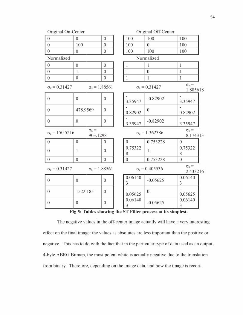
54
Original On-Center Original Off-Center 0 0 0 100 100 100 0 100 0 100 0 100 0 0 0 100 100 100 Normalized Normalized 0 0 0 1 1 1 0 1 0 1 0 1 0 0 0 1 1 1
σc = 0.31427 σs = 1.88561 σc = 0.31427 σs = 1.885618
0 0 0 -3.35947 -0.82902 -
3.35947
0 478.9569 0 -0.82902 0 -
0.82902
0 0 0 -3.35947 -0.82902 -
3.35947
σc = 150.5216 σs = 903.1298 σc = 1.362386 σs =
8.174313 0 0 0 0 0.753228 0
0 1 0 0.753228 1 0.75322
8
0 0 0 0 0.753228 0
σc = 0.31427 σs = 1.88561 σc = 0.405536 σs = 2.433216
0 0 0 0.061403 -0.05625 0.06140
3
0 1522.185 0 -0.05625 0 -
0.05625
0 0 0 0.061403 -0.05625 0.06140
3
Fig 5: Tables showing the ST Filter process at its simplest.
The negative values in the off-center image actually will have a very interesting
effect on the final image: the values as absolutes are less important than the positive or
negative. This has to do with the fact that in the particular type of data used as an output,
4-byte ABRG Bitmap, the most potent white is actually negative due to the translation
from binary. Therefore, depending on the image data, and how the image is recon-
55
structed, either the corners will be bright and the cells above and to the sides will be dim-
mer, or else the opposite will be true. An additional step, not present in Karagoz et al,
was the second normalization of the data; the reason for this addition is in chapter 4.
While this works well as a proof of concept, no particular filter system that is only
this large would be of practical value, at least at first glance. This led to the discovery,
over the course of the development of the final product, that the real system must divide
the image into parts that are not much larger than this in order to function, as the values
for the Gaussian equation very quickly round to zero in Java. Therefore, this paper test
could have been one of the most significant pieces of the puzzle, despite its apparent sim-
plicity. As stated earlier, there was no real code written for this part: all calculations per-
formed by hand, so no code exists for this, aside from the formulae mentioned previ-
ously. The code for the rest of the iterations, where it survives, will be included in Ap-
pendix A.
Model 2: Using The “Lena” Image
The next stage in the process was to see how well the ST-filter system performed
on a real image. Since the output device required a specific type of data as input, and
while the input was considerably more flexible, it was determined that the entire process
should follow a single type of file thru the entire process. For this reason, an image that
was preferably square, black and white, and of type bitmap was required. In addition,
Gaussian distortion is primarily concerned with edge definition and detection, which is
what a functional human eye captures; an image containing multiple well-defined edges
would be ideal. As to the resolution, this was not as important to the initial screening
56
process for an image, as at the time, perception led to the belief that this was not im-
portant. Later, after the system was developed, the revelation came about that the image
we chose was much higher resolution than would the device itself used. As a result of
this, the timing now had much less weight, but also held more interest compare to the
timing goals that were set, and were nearly met in theory, as the system could then handle
much higher-resolution images than initially believed.
The chosen image was a square, black and white photograph of a young girl,
which met with the above criteria. It also has much in terms of fine-level detail (the
feathers in the hat for example) that allows for the determination of how much detail loss
existed after processing. Though this is slightly subjective, it does allow for an additional
level of fine-tuning the device, especially when discussing the radius function, one of the
major elements of the final version of this program. In addition, the focus of the image is
the face of a young woman, and facial recognition is one of the most important aspects of
the human visual system: while actual recognition of who the person is does not matter,
the ability of the person to recognize that they are seeing a human face is vitally im-
portant. Below, the image eventually selected, and it is included to allow for a base line
that the user can draw their own judgment on the effectiveness of the various image ma-
nipulation techniques. The image has a long history in computer science as a baseline
image, and comes originally from Playboy magazine.
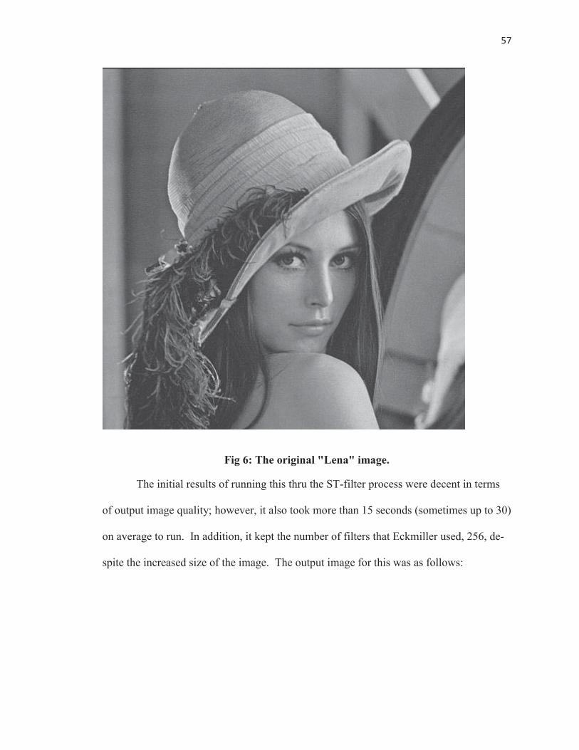
57
Fig 6: The original "Lena" image.
The initial results of running this thru the ST-filter process were decent in terms
of output image quality; however, it also took more than 15 seconds (sometimes up to 30)
on average to run. In addition, it kept the number of filters that Eckmiller used, 256, de-
spite the increased size of the image. The output image for this was as follows:
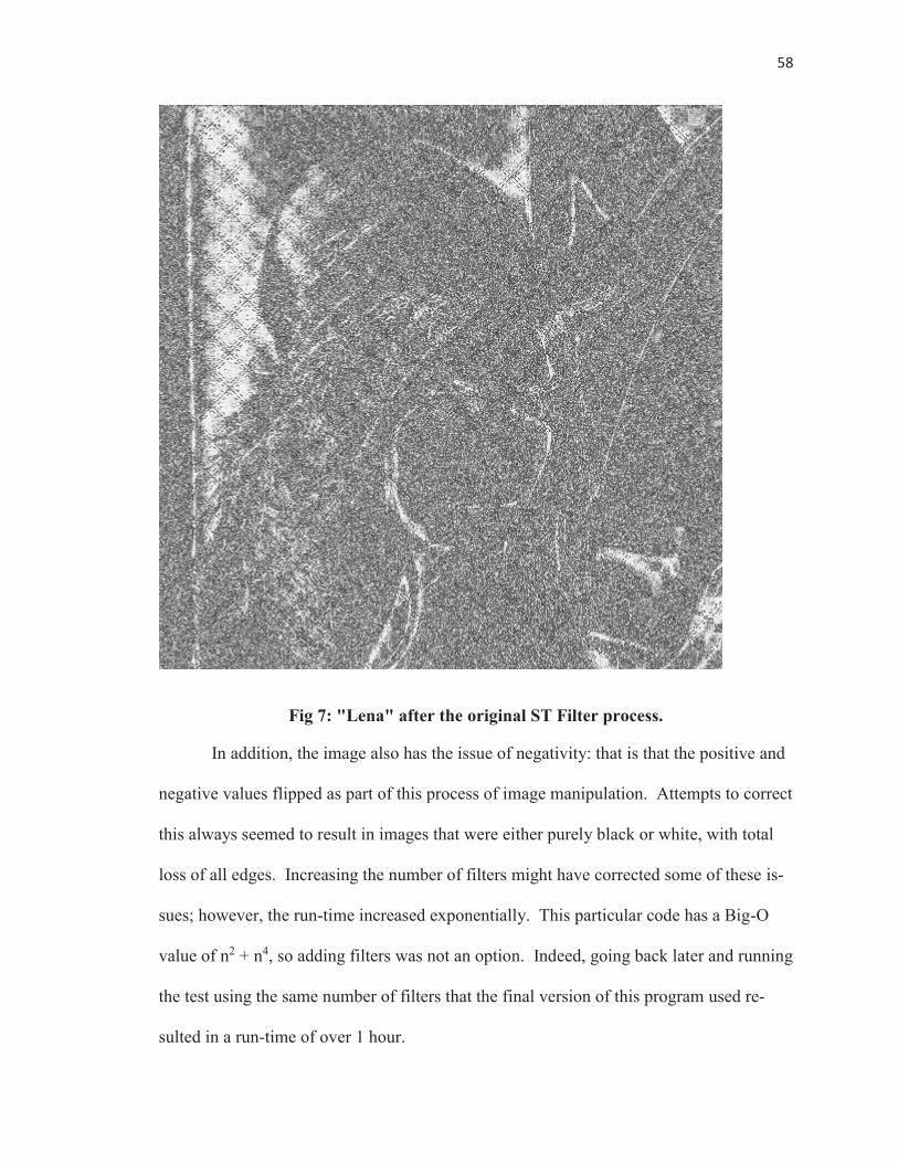
58
Fig 7: "Lena" after the original ST Filter process.
In addition, the image also has the issue of negativity: that is that the positive and
negative values flipped as part of this process of image manipulation. Attempts to correct
this always seemed to result in images that were either purely black or white, with total
loss of all edges. Increasing the number of filters might have corrected some of these is-
sues; however, the run-time increased exponentially. This particular code has a Big-O
value of n2 + n4, so adding filters was not an option. Indeed, going back later and running
the test using the same number of filters that the final version of this program used re-
sulted in a run-time of over 1 hour.
59
An important design feature of this system, however, is that unlike the versions
seen in both Karagoz and Eckmiller, this version was size-independent: that is it could be
run altering the number of filters, both horizontal and vertical, independent of the size of
the input image. Therefore, the image itself became unimportant, and the focus could re-
main on edge detection, rather than finding the magic ratio of the number of filters versus
image clarity.
Model 3: The Addition Of The Radius
One of the first improvements added to the system came after realizing the afore-
mentioned fact that all of the values returned outside of a given radius from the center of
the image are zero, and were not having any effect on the overall outcome of the image,
at least in this version of the design. Therefore, in order to reduce the running time, the
addition of a new, very small subroutine to the process that made it so it would only go
out a certain distance from the center point. This finite radius function simply divides the
total size of the image by the number of filters, and uses that to prevent overlap, reducing
the number of times that the image goes thru the ST-filter loop. While it does not affect
the Big-O time of the image, it significantly reduced the number of iterations.
This resulted in a significantly shorter run time of only 541ms. While this is still
well above the goal speed of 33ms, given the hardware limits, and the size of the image
compared to what would eventually come about, this was extremely promising. As dis-
cussed, this is also a question of resolution, as “Lena” is a much higher resolution image
than the end device itself will use. A second version that allowed for overlap was also
developed. This version, while slightly slower, clocking in at 837ms, produced an image
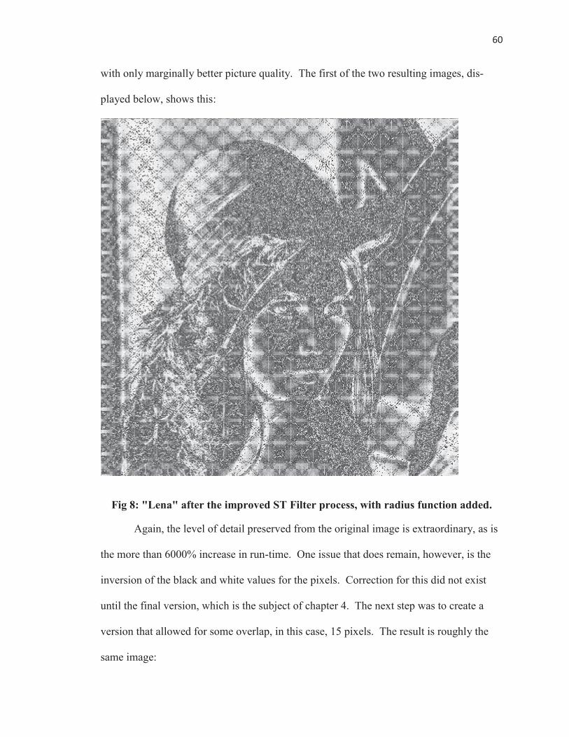
60
with only marginally better picture quality. The first of the two resulting images, dis-
played below, shows this:
Fig 8: "Lena" after the improved ST Filter process, with radius function added.
Again, the level of detail preserved from the original image is extraordinary, as is
the more than 6000% increase in run-time. One issue that does remain, however, is the
inversion of the black and white values for the pixels. Correction for this did not exist
until the final version, which is the subject of chapter 4. The next step was to create a
version that allowed for some overlap, in this case, 15 pixels. The result is roughly the
same image:
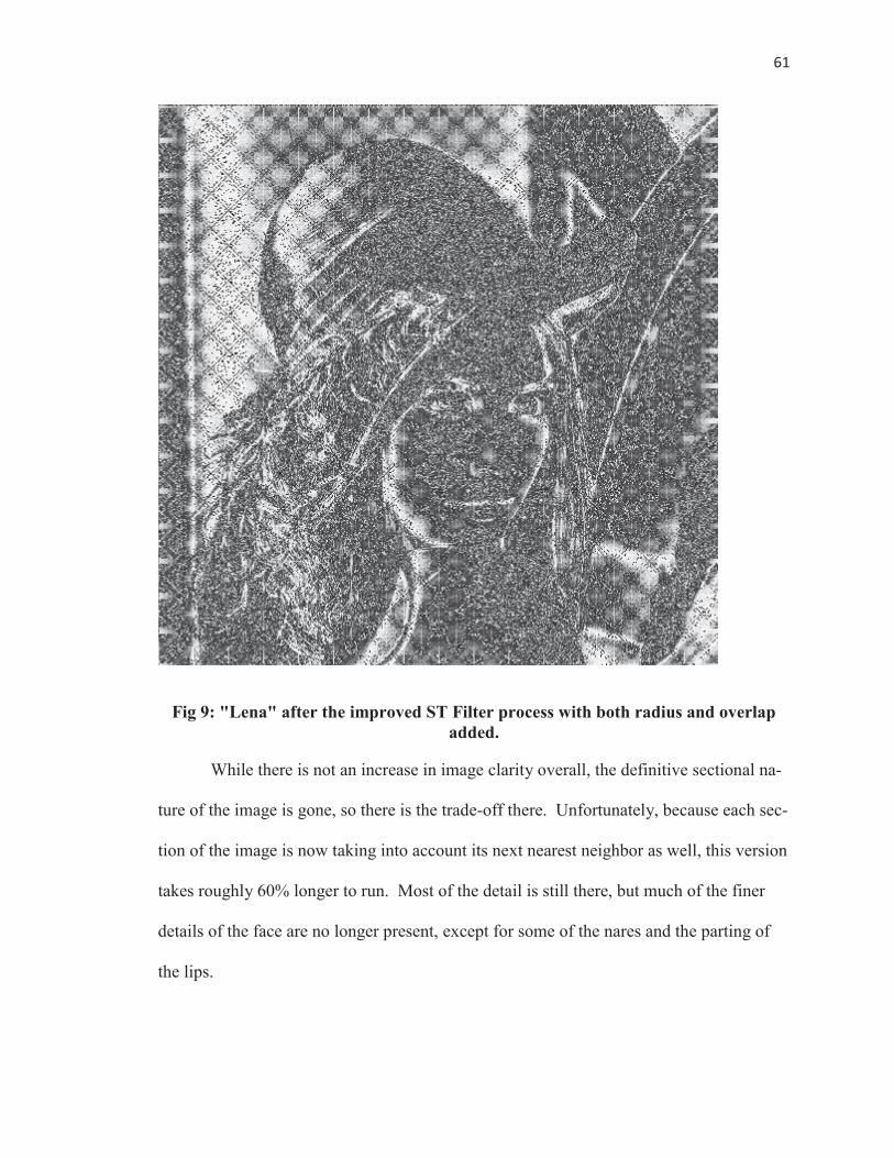
61
Fig 9: "Lena" after the improved ST Filter process with both radius and overlap added.
While there is not an increase in image clarity overall, the definitive sectional na-
ture of the image is gone, so there is the trade-off there. Unfortunately, because each sec-
tion of the image is now taking into account its next nearest neighbor as well, this version
takes roughly 60% longer to run. Most of the detail is still there, but much of the finer
details of the face are no longer present, except for some of the nares and the parting of
the lips.
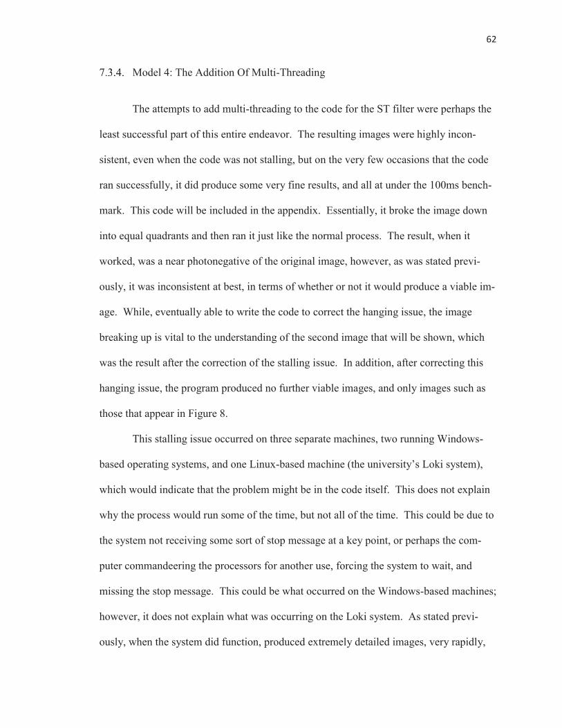
62
Model 4: The Addition Of Multi-Threading
The attempts to add multi-threading to the code for the ST filter were perhaps the
least successful part of this entire endeavor. The resulting images were highly incon-
sistent, even when the code was not stalling, but on the very few occasions that the code
ran successfully, it did produce some very fine results, and all at under the 100ms bench-
mark. This code will be included in the appendix. Essentially, it broke the image down
into equal quadrants and then ran it just like the normal process. The result, when it
worked, was a near photonegative of the original image, however, as was stated previ-
ously, it was inconsistent at best, in terms of whether or not it would produce a viable im-
age. While, eventually able to write the code to correct the hanging issue, the image
breaking up is vital to the understanding of the second image that will be shown, which
was the result after the correction of the stalling issue. In addition, after correcting this
hanging issue, the program produced no further viable images, and only images such as
those that appear in Figure 8.
This stalling issue occurred on three separate machines, two running Windows-
based operating systems, and one Linux-based machine (the university’s Loki system),
which would indicate that the problem might be in the code itself. This does not explain
why the process would run some of the time, but not all of the time. This could be due to
the system not receiving some sort of stop message at a key point, or perhaps the com-
puter commandeering the processors for another use, forcing the system to wait, and
missing the stop message. This could be what occurred on the Windows-based machines;
however, it does not explain what was occurring on the Loki system. As stated previ-
ously, when the system did function, produced extremely detailed images, very rapidly,
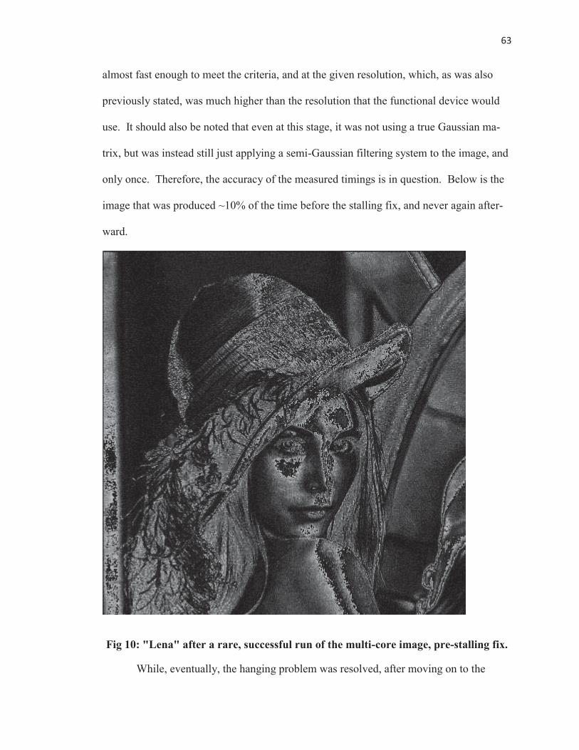
63
almost fast enough to meet the criteria, and at the given resolution, which, as was also
previously stated, was much higher than the resolution that the functional device would
use. It should also be noted that even at this stage, it was not using a true Gaussian ma-
trix, but was instead still just applying a semi-Gaussian filtering system to the image, and
only once. Therefore, the accuracy of the measured timings is in question. Below is the
image that was produced ~10% of the time before the stalling fix, and never again after-
ward.
Fig 10: "Lena" after a rare, successful run of the multi-core image, pre-stalling fix.
While, eventually, the hanging problem was resolved, after moving on to the
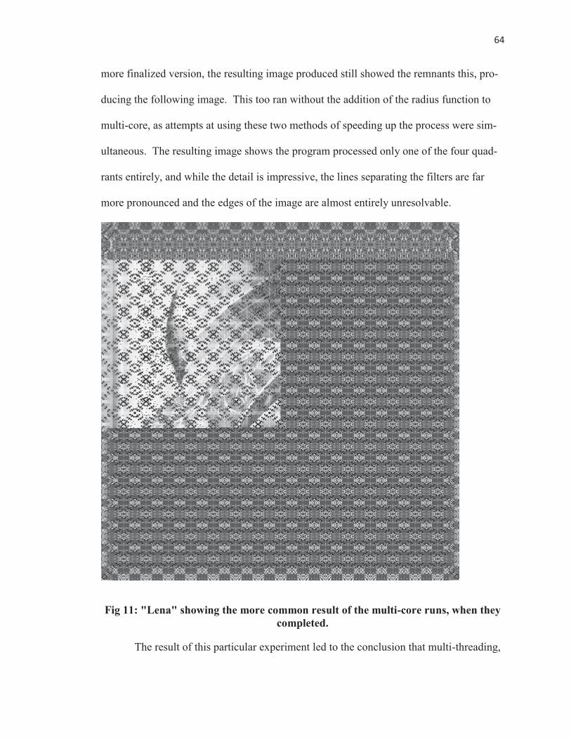
64
more finalized version, the resulting image produced still showed the remnants this, pro-
ducing the following image. This too ran without the addition of the radius function to
multi-core, as attempts at using these two methods of speeding up the process were sim-
ultaneous. The resulting image shows the program processed only one of the four quad-
rants entirely, and while the detail is impressive, the lines separating the filters are far
more pronounced and the edges of the image are almost entirely unresolvable.
Fig 11: "Lena" showing the more common result of the multi-core runs, when they completed.
The result of this particular experiment led to the conclusion that multi-threading,
65
at this point, was not yielding the desired results that, and so a different path became nec-
essary, and one that came from a more basic source, rather than the ambition. Indeed,
since the hardware of the final device is unknown, to assume that it will natively support
multi-threading is an assumption that could lead to the entire process becoming unusable.
Model 5: The Addition Of Pipeline
The pipeline came about at the same time that the revelation of the lack of true
Gaussian filters in the system revealed itself. Therefore, those involved in the project de-
termined that a true-two staged, pipelined system should be created, and the entire project
started over from little more than scratch: a lot of components could be reused, but not in
the form that they existed currently. The result of the initial discussions also revealed
that the run-time of this system would be significantly slower as a result, given that it
would now perform, essentially, twice the work. This led to the necessitation of the pipe-
lining system used in the final models, and serves as the turning point between the older-
model systems and the new systems, as the first system produced using pipelining is, in
all respects, the final 1-to-1 version of the system.
Final Models
The presented final models are those currently used actively for experimentation,
and proposed for use in the final system. They are all relatively small, and can all run
from the same testing script. In essence, all three of them perform the same actions, the
only major difference stems from how they reassemble the image data after each iteration
of the Gaussian filter loop.
66
Overview
As was stated in Chapter 2, this particular design is a modification of the design
found in the paper by Karagoz et al, but only to a point. One major modification is the
exclusion of the NLIF, due to this project’s scope rendering it unnecessary. The second
has to do with the improvements made specifically to run-time and architecture, as were
discussed in the specifics of the prototypes in Chapter 3. The following sections will dis-
cuss which of these improvements showed enough promise to keep, and how the modifi-
cations progressed to meet the requirements decided upon in the final design.
In total, the results of the research necessitated the creation of three designs based
on the original prototypes, each of them harnessing aspects from all prototypes to create
their respective output images. Each comes with benefits and trade-offs, as is to be ex-
pected. There are several universal aspects to each version, however. To start, each ver-
sion first breaks the image into smaller, discrete sections to be processed individually (a
technique that although run in a single thread here, was developed based on the work
with multi-threading, and could be done in that manner with a few minor modifications).
Each version then uses a modification of the ratio of ST filters to image sections. The
key differences between the three versions stems from these aspect ratios, namely the
number of filters into which each image section feeds.
In addition, due to several discoveries about how the process should work, the
number of filters used dramatically increased, from 256 to 65536. This was done to in-
crease the image clarity overall, as well as due to the fact that with the improvements
made, the radius over which each filter functions was significantly reduced. After a ra-
dius of more than about four pixels, the entirety of the image reduces to no more than a
67
sea of black, because of the exponential portion of the function. This caused several ben-
efits, as can be seen in the sample images for each ratio: notably, the lack of any of the
radius lines, as the number of pixels wasted on the radius reduces to zero. The second is
an increase in clarity, as the amount of noise from pixels that are extremely off-centered
reduces to near-zero levels, as well.
1-To-1 Ratio
This particular ratio evolved from the basics of both Karagoz et al and Eckmiller
et al, and each section of the original image feeds into a single ST filter system, with no
overlap. Essentially, this is still the most basic prototype, though modified to fit into the
pipeline method, as well as 3D-ADoG. As was stated, this is the radius function in full
effect, but without allowing for overlap. The output image still contains the “photo-nega-
tive” quality of the earlier prototypes, but there are numerous key differences. First, most
edges are fantastically preserved, showing the same, or near the same, level of detail as
the original radius function, but at a slightly higher speed. Given that the functions used
are significantly more complex (the original was, in actuality a single-stage ST filter sys-
tem, whereas this uses the true matrix function and two stages), the minimal increase in
speed is acceptable. The second, as was just mentioned is the speed, which due to the
pipelining, sees an overall reduction compared to the original radius function, when con-
sidering the effect that it has at each stage, as well as the number of steps required for
each stage.
There are downsides, however. In addition to the photo negativity, the image is
also still quite grainy, as each pixel, despite the finite radius, still carries over some ef-
fects from every other pixel around it. In addition, while the image preservation is better,
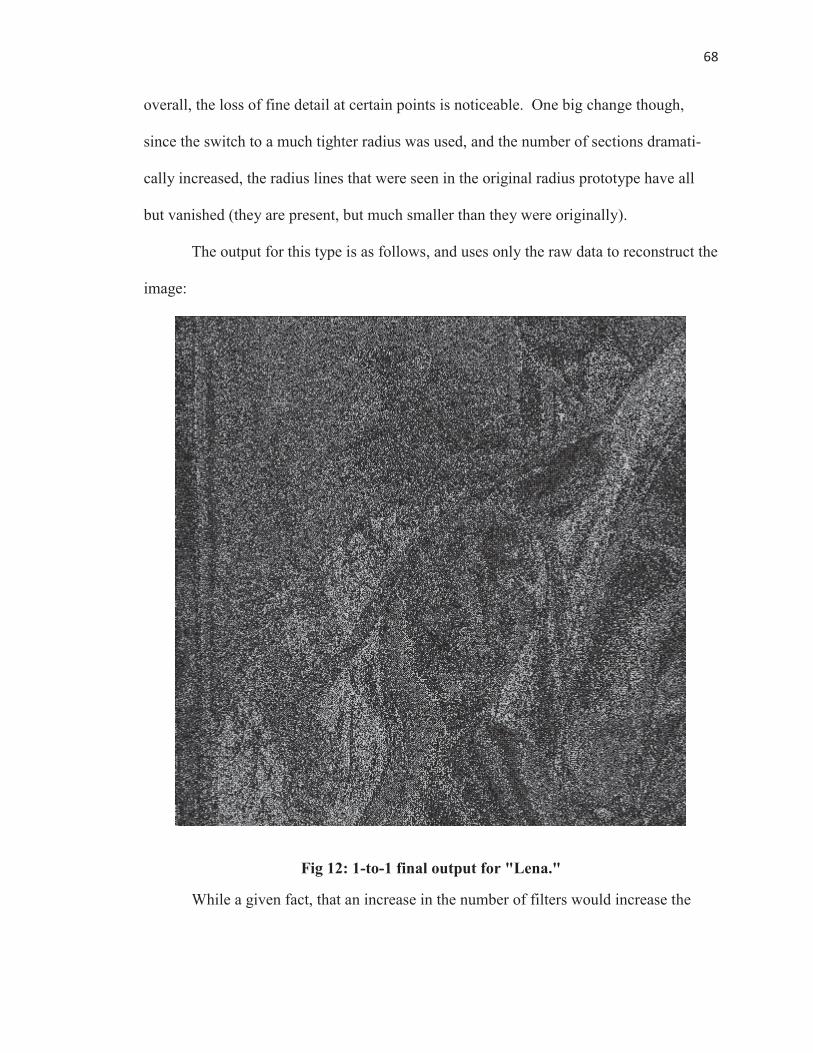
68
overall, the loss of fine detail at certain points is noticeable. One big change though,
since the switch to a much tighter radius was used, and the number of sections dramati-
cally increased, the radius lines that were seen in the original radius prototype have all
but vanished (they are present, but much smaller than they were originally).
The output for this type is as follows, and uses only the raw data to reconstruct the
image:
Fig 12: 1-to-1 final output for "Lena."
While a given fact, that an increase in the number of filters would increase the
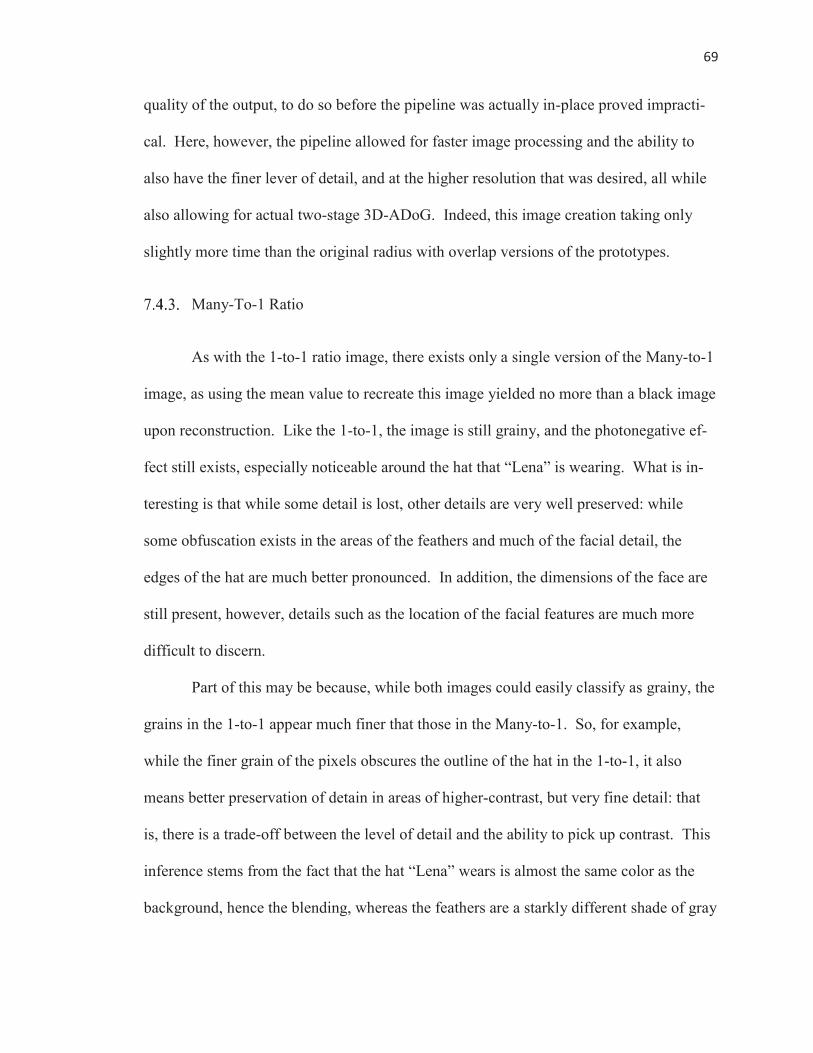
69
quality of the output, to do so before the pipeline was actually in-place proved impracti-
cal. Here, however, the pipeline allowed for faster image processing and the ability to
also have the finer lever of detail, and at the higher resolution that was desired, all while
also allowing for actual two-stage 3D-ADoG. Indeed, this image creation taking only
slightly more time than the original radius with overlap versions of the prototypes.
Many-To-1 Ratio
As with the 1-to-1 ratio image, there exists only a single version of the Many-to-1
image, as using the mean value to recreate this image yielded no more than a black image
upon reconstruction. Like the 1-to-1, the image is still grainy, and the photonegative ef-
fect still exists, especially noticeable around the hat that “Lena” is wearing. What is in-
teresting is that while some detail is lost, other details are very well preserved: while
some obfuscation exists in the areas of the feathers and much of the facial detail, the
edges of the hat are much better pronounced. In addition, the dimensions of the face are
still present, however, details such as the location of the facial features are much more
difficult to discern.
Part of this may be because, while both images could easily classify as grainy, the
grains in the 1-to-1 appear much finer that those in the Many-to-1. So, for example,
while the finer grain of the pixels obscures the outline of the hat in the 1-to-1, it also
means better preservation of detain in areas of higher-contrast, but very fine detail: that
is, there is a trade-off between the level of detail and the ability to pick up contrast. This
inference stems from the fact that the hat “Lena” wears is almost the same color as the
background, hence the blending, whereas the feathers are a starkly different shade of gray
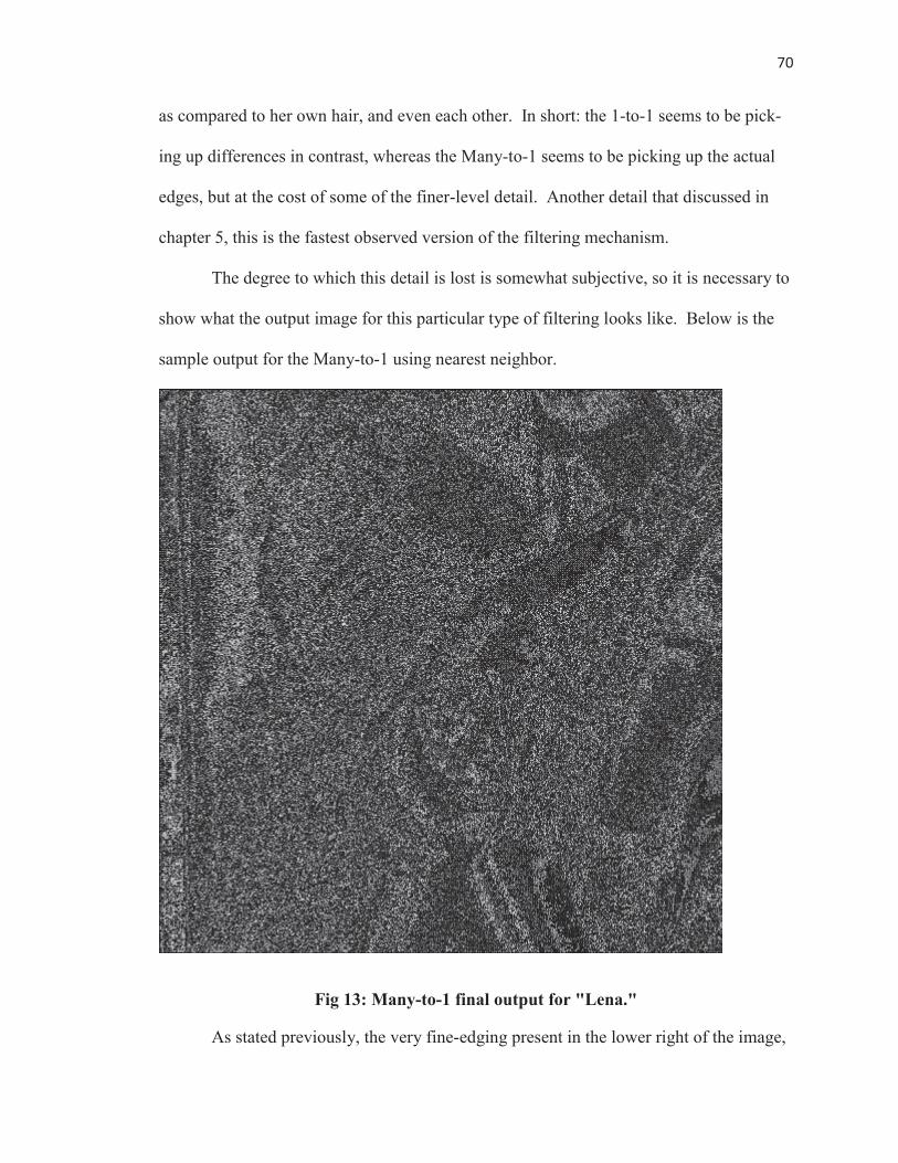
70
as compared to her own hair, and even each other. In short: the 1-to-1 seems to be pick-
ing up differences in contrast, whereas the Many-to-1 seems to be picking up the actual
edges, but at the cost of some of the finer-level detail. Another detail that discussed in
chapter 5, this is the fastest observed version of the filtering mechanism.
The degree to which this detail is lost is somewhat subjective, so it is necessary to
show what the output image for this particular type of filtering looks like. Below is the
sample output for the Many-to-1 using nearest neighbor.
Fig 13: Many-to-1 final output for "Lena."
As stated previously, the very fine-edging present in the lower right of the image,
71
where the feathers from the hat overlap with her hair, is at least as blurred as the top of
the hat in the 1-to-1 image. In addition, while the vague outlines of the areas of her face
are present, it is somewhat more difficult to discern than the 1-to-1 counterpart is.
Many-to-Many
This would be the source of the most trade-offs in terms of running time versus
image quality, when using mean. In fact, as was demonstrated in chapter 5, it runs at just
under four times slower than its counterpart does when using. The produced results,
however, demonstrate why, if there exists the possibility for a reduction in the image res-
olution, the superiority of this version is apparent. In the first image, that using mean, not
only are details wonderfully preserved so too are light-level gradients. Again, a portion
of this is subjective as to the desired level of detail. The second image is that using the
nearest neighbor to reconstruct the image. The quality seems on-par with that seen when
unsing the same reconstruction method in the Many-to-1 model. This would indicate that
the reconstruction process has some effect on the image quality, whereas the mapping has
an effect on the speed.
In the first image, as stated previously, the detail is very well preserved, and edges
can be seen in amazing contrast to their surroundings. The second image is still a slight
improvement, however, the finer detail, as in Many-to-1 is still lost when reconstruction
of the image occurs. While there is still some light/dark inversion, compared to the true
Many-to-1 system, it is much less severe.
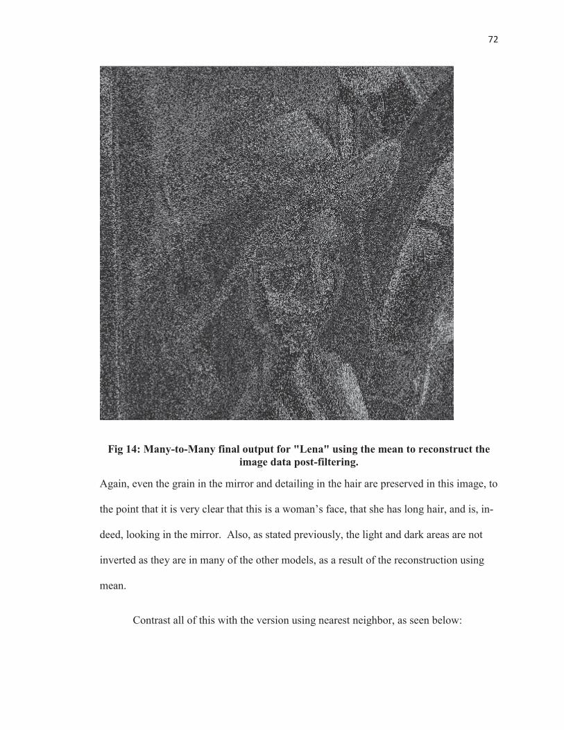
72
Fig 14: Many-to-Many final output for "Lena" using the mean to reconstruct the image data post-filtering.
Again, even the grain in the mirror and detailing in the hair are preserved in this image, to
the point that it is very clear that this is a woman’s face, that she has long hair, and is, in-
deed, looking in the mirror. Also, as stated previously, the light and dark areas are not
inverted as they are in many of the other models, as a result of the reconstruction using
mean.
Contrast all of this with the version using nearest neighbor, as seen below:
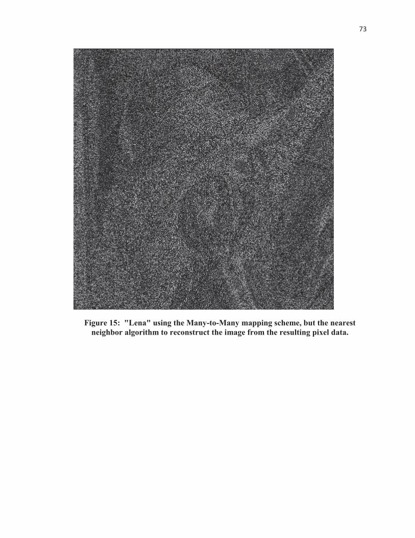
73
Figure 15: "Lena" using the Many-to-Many mapping scheme, but the nearest neighbor algorithm to reconstruct the image from the resulting pixel data.
74
While the light/dark inversion is nowhere near so bad as in Many-to-1, it is still
present. However, the level of detail still seems higher than in Many-to-1, though this is
partiallys subjective. However, the mirror’s outline, as well as many of the edges on both
the face and the hat are well-preserved, only the extremely fine details of the hair are to-
tally obstructd.
1-To-Many
While discussion about this model occurred at length and the implementation the-
orized, this particular model never came about for several reasons. First, the issue of time
requirement: the other models showed more promise, and were already mostly functional
by the time of the bulk of this model’s discussion. Second, and perhaps most important,
was the difficulty discovered in defining this particular model in a computer simulation.
While conceptually, this is not a difficult concept to grasp, see chapter 4, the overall use
of such a model in the current system would have resulted in a lot of redundancy and run-
time padding, rather than achieving anything different from the 1-to-1 model. The reason
here is that the ratio dictates each image section’s use in conjunction with only itself, and
not with any other filters. Were it used with other image sections, this would simply be-
come a Many-to-Many model. A second problem occurs in that this all becomes highly
redundant, since it would necessitate the use of many independent filters on the same,
static, image section: many filters producing identical results. This would only serve to
increase the run-time while producing an image that, essentially, is nigh identical to the
1-to-1 model.
As discussed in chapter 4, while this mapping system is very similar to the Many-
to-1 system, for this particular project it makes no sense to use it, and, unlike the Many-
75
to-1 system, there was no way to bend the definitions. That is the only reason the Many-
to-1 system is available for use: the slight bending of the definitions “many” and “one”
such that each image section as a whole is used only once, but parts of it are used multi-
ple times, so as to avoid it turning into a Many-to-Many or a 1-to-1. However, this map-
ping does not allow for any such flexing without total breakage, it is much more rigid. In
short, while an interesting and abstract concept, it exists here only to round out the four
types of mapping that exist, and its implementation in this project is non-existent, except
as a thought experiment in how to accomplish such a design.
76
CHAPTER 8: CONCLUSIONS AND FUTURE
WORK
Conclusions
In this project, essentially three functional software prototypes for the inner-work-
ings of a retinal prosthesis, specifically the initial image processing, have come into be-
ing. It is still necessary that much work and refinement continue on these prototypes, as
none of them met the timing requirements initially laid out. However, it is also necessary
to point out that the images coming out of each of these prototypes are remarkably simi-
lar to the reconstructed images seen in many other papers on this subject, specifically Ka-
ragoz et al [1], and Eckmiller et al [2]. To that end, this is a success as a project, even
without the NLIF portion.
Indeed, this thesis demonstrates that one aspect ignored by both of those authors:
the question of whether how the ST filters are mapped to the image has an effect on the
speed or output. As this thesis demonstrates, this is indeed a very important descision, as
a definitive trade-off between level of detail and the speed of the image was seen. This
makes sensefrom a logical standpoint, as mapping techniques require different levels of
work to be realized. There was also evidence that with some future work, it may become
feasible to overcome the speed issues. As discussed in chapter 6, the fastest model also
produced the least amount of detail for the ST filter output. However, there also seems to
be something to be said for the methods used to reconstruct the image.
77
While much of the focus was on the speed of the image processing, the im-
portance of the image detail cannot be ignored. To that end, using mean on most fre-
quently produced a much crisper overall image, while nearest neighbor produced a less
detailed image, and in the instance where both were used on the same mapping scheme,
actually seemed slower. Additionally, whenever nearest neighbor was used, there was
some light/dark inversion in the image. Though this also occurred while using mean,
when using mean in conjunction with the Many-to-Many mapping, this effect was elimi-
nated. The next step would be to try both outputs in the NLIF, to see if the sharpness and
detail are retained thru that phase, and can be transmitted to the electrodes actually at-
tached to the eye.
While the NLIF is nonexistent here, and though it is a major component according
to much of the research, its functionality is questionable to this project, as it seems to be
unimportant to the work of this thesis. The crux of the project was to determine if the
mapping scheme and image reconstruction methods had any effect on overall speed and
image quality, and this was observed. The NLIF, however, would seem to function more
as a sort of replacement to the optic ganglion itself, below the layers of the retina, and
possibly substitute for the optic nerve, and the design is static, and not affected by either
mapping r reconstruction methods. This is not to say that omission of the NLIF is a good
thing, merely that the necessity of such a device remains questionable to the scope of this
project.
A final issue with the images as they stand is the quantification of clarity. Again,
the images seen are not what the output images would actually be, but rather the inputs to

78
the NLIF, and as such, no refinement has occurred. This makes it very difficult to quan-
tify using the standard method of contours, since there is too much noise in the images
themselves. This makes the creation and inclusion of the NLIF to this model all the more
important. As it stands, the clearest image, Many-To-Many, still requires a countour fil-
tering of 50% higher than the original image to even approach the same level of clarity.
Some of these issues would be corrected by NLIF, not only because of the manner in
which it functions, but also because of the tuning of the NLIF, which will reduce the
amount of noise.
Future Work
While there was much accomplished in this project, it would be naïve to believe
that it represents anything remotely close to a comprehensive attempt at this work. This
thesis should essentially act as a gateway for how to proceed in the future in this particu-
lar line of thought, and to that end, there are numerous avenues that require further explo-
ration.
Radius Function
Given the importance that this function has had on the overall functioning of the
ST filter process, arguably second only to pipelining in terms of timing and effect, this
shows promise in the future versions of this design. One addition mentioned previously
in the paper was the idea that the image sections do not need to be symmetrical, as they
are here, but rather can conform to the specific shapes required by each user. In so doing,
it would be possible to allow for an ST filter system that is truly unique to each user’s ret-
ina and visual preference.
79
Pipelining And Multi-Threading
Streamlining the process in order to increase speed of the overall device was a key
part of this thesis, as well as an area of major focus, but there is far more that can be
done, including optimizing the pipeline for better multithreading. While the design of the
pipeline shown previously does lend itself quite well to multithreading, image reconstruc-
tion never occurred, at least not successfully, and so this particular area cannot receive
coverage as deserved. Indeed, the pipelining aspect quickly became the single most-im-
portant aspect of the project after the mapping scheme, as it dramatically decreased the
runtime, but also one of the least utilized, and not to its full potential, at least not without
the addition of multithreading.
As to multithreading, when this project first started, there was no question that
multithreading was an unattainable goal. However, as the project advanced, this concept
very quickly took a much more important role, as the speedups promised were too tanta-
lizing to ignore. As seen above, the results never lived up to expectations, at least in this
project, so this area requires significantly more time, and probably from a more experi-
enced programmer, to fully realize. Especially with the revelation the final product could
very easily incorporate at least a dual, if not quad-core processor, the utilization of multi-
threading to its full potential becomes and even more important feature to develop: it will
allow for larger, more complicated images to go thru the filtering process faster, preserv-
ing more detail, and more acutely reproducing the lost vision, and it integrates very natu-
rally into the multi-threading schema.
With the exception of NLIF, this is probably the most lamented lost piece to the
puzzle that was this project, and one that would require great attention from those who
80
continue in this work. Since the confirmation of a multi-core prototype, as well as the
continued miniaturization of all hardware in general, this prospect comes closer and
closer to a reality, and deserves more attention. While the initial goal of 30 frames per
second was set, based on the limits of biological response, aside from power consumption
there is no reason not to exceed this goal. A proposed manner to combine multi-thread-
ing with the pipeline: each core dedicated to a separate function; one to breaking
down/processing the first image, one to the creation of the second image, one to the
breaking down/processing of the second image, and the final core to the NLIF itself.
Output
In general, the outputs come with several trade-offs that must be considered. As
to aesthetics, it is up to the individual user preference in the end, however, the Many-to-
Many implementation seems to preserve detail the best, but with the slowest running time
on the hardware used. Ideally, to have the detail level seen with the Many-to-Many im-
plementation using mean, but the speed of the Many-to-1 implementation could exist.
More tests, and specifically in vivo tests, are required in order to demonstrate the true ef-
fectiveness of these schemes, as the current tests are far too isolated in terms of run-time
and hardware, to convey their effectiveness and speed with any real meaning, outside of
baseline comparison. One known fact, however, is that with the smaller images that the
real prototype uses, these schemas should all run significantly faster, as they will require
fewer filters, run over fewer pixels, and so run-times should decrease dramatically with
each reduction in size. Add to this the prospect on the NLIF, and the only item left to test
is the particular user preference.
81
Eventually, with everything else equal, the three schemas should function at rela-
tively fast enough speeds that the distinguishing factor would be the user’s preference.
Additionally, one avenue not explored in this project is what would occur with different
schemes used at differing stages: for example, the first-level ST filter used a Many-to-
Many scheme, and the second level used a Many-to-1 scheme. Would this have a major
effect on either clarity or on speed? This might better simulate real eye function, as the
functionality of some of the cells located deeper in the retina remains unknown, and
might not function simply as a mirror to the outer layers.
Also, as stated, the outputs seen are meant to be visual interpretations of the data
which would go into the NLIF, and so are not actually representative of how the final
output will appear. However, more can be done to smooth this data out before it goes
into the NLIF, which would allow for more contour matching compatability. As it cur-
rently stands, to try and quantify the image clarity compared to the original is not practi-
cal, since the noise created by the Gaussian filter process is fairly extreme, with numer-
ous artifacts. This is true for all four outputs, but especially true for those using the near-
est neighbor algorithm. The best seen so far required an decrease in sensitivity by almost
50%.
Universality
A secondary goal here was the demonstration that using current hardware, the
computational language requirement put forward by Eckmiller, that such programs can
exist only in C or Basic, no longer carry relevancy. While this project did not meet the
timing requirements initially set out, it did demonstrate that such assertions are likely
82
false. The only hurdle left to this project is implementation of a live-system to test the al-
gorithms in-vivo. As stated previously, the images used are significantly larger than
those that such a device uses, indicating that the goal is within reach when using an im-
age at the resolution that Eckmiller used. Additionally, the test environments existed on a
computer, that while much more powerful than what the device would use, did not have
designs for such a device specifically when manufactured, nor was it running the program
for the device exclusively.
To this end, the use of Java indicates a step toward universality: despite the fact
that it ran in a Windows environment, the program should be portable to any device, as
the language used will not change based on the operating system, and is theoretically uni-
versal to any JVM. Indeed, to port this program to a device should require only minor
tweaks to either how the program accesses the necessary files in the file structure, as op-
posed to having to re-write whole segments based on the hardware (Basic/Machine Code)
or the command structure of the operating system (C/C++). To that end, this program ex-
ists more as a proof of concept than a polished and final version, as it still requires testing
in vivo, however, the universality aspects of it exist, and only require some further test-
ing.
NLIF
As previously stated, the NLIF was not necessary to this design; however, the
functionality of such a piece of software is beyond doubt. Indeed, it would allow for re-
placement of vision beyond the current limits, and possibly into true blindness. To do
this, however, would require an understanding of the human visual system that is beyond
what currently exists. The NLIF, in essence, would simulate the responses that already
83
exist in the ganglion; sending spikes of information to the brain, and letting the brain de-
code such spikes. The issue here becomes whether the brain is still capable of such a pro-
cess after prolonged absence or even the nonexistence since birth, of such spikes, as sev-
eral authors have pointed out that either the brain becomes non-responsive, or that the
signals are slowly adapted to by the brain in such a way that they cease to produce visual
stimuli [5].
Quiroga et al predict something even more fascinating, if such a device is ever re-
fined to the point of proposed functionality. They propose that such a device could move
beyond the simple retinal prosthesis, and allow meaningful machine-human interaction,
as well as serve to recreate lost limbs through brain-controlled prosthesis [8]. It makes
sense to see such potential, given the description of how the NLIF should work: after all,
if the ability to simulate one type of nerve exists, then the applicability to other types
should present slightly less of a problem, as it would not start from scratch. Again, how-
ever, exaggerating the difficulties in understanding both the functional complexity and
the importance of such a device proves difficult, especially since evidence shows that it is
variability in the firing rates that produces information [8], and most of the models pre-
sented here are designed to present a nigh-constant stream of information.
Appendix i
APPENDIX A: Works Cited
[1] I. Karagoz and M. Ozden, "Adaptive Artificial Retina Model to Improve Perception Quality of Retina Implant Recipients," in 2011 4th International Conference on Biomedical Engineering and Informatics(BMEI), Shanghai, 2011.
[2] R. Eckmiller, D. Neurmann and O. Baruth, "Tunable Retina Encoders for Retina Implants: Why and How," Journal of Neural Engineering, vol. 2, no. 2005, pp. S91-S104, 22 February 2005.
[3] W. Liu, K. Vichienchom, M. Clements, S. C. DeMarco, C. Hughes, E. McGucken, M. S. Humayun, E. de Juan, J. D. Weiland and R. Greenberg, "A Neuro-Stimulus Chip with Telemetry Unit for Retinal Prosthetic Device," IEEE Journal of Solid-State Circuits, vol. 35, no. 10, pp. 1487-1497, 10 October 2000.
[4] S. Nirenberg and C. Pandarinath, "Retinal Prosthetic Strategy with the Capacity to Restore Normal Vision," in Proceedings of the National Acadamy of Sciences of the United States of America, New York, 2012.
[5] J. O. Winter, S. F. Cogan and J. F. Rizzo, "Retinal prostheses: Current Challenges and Future Outlook," Journal of Biomaterials Science Polymer Edition, vol. 18, no. 8, pp. 1031-1055, February 2007.
[6] D. K. Freeman and S. I. Fried, "Multiple Components of Ganglion Cell Desensitization in Response to Prosthetic Stimulation," Journal of Neural Engineering, 1 February 2011.
[7] E. Orhan, "The Leaky Integrate-and- Fire Neuron Model," Rochester, 2012.
[8] R. Q. Quiroga and S. Panzeri, "Extracting Information From Neuronal Populations: Information Theory and Decoding Approaches," Nature Reviews Neuroscience, vol. 10, pp. 173-185, March 2009.
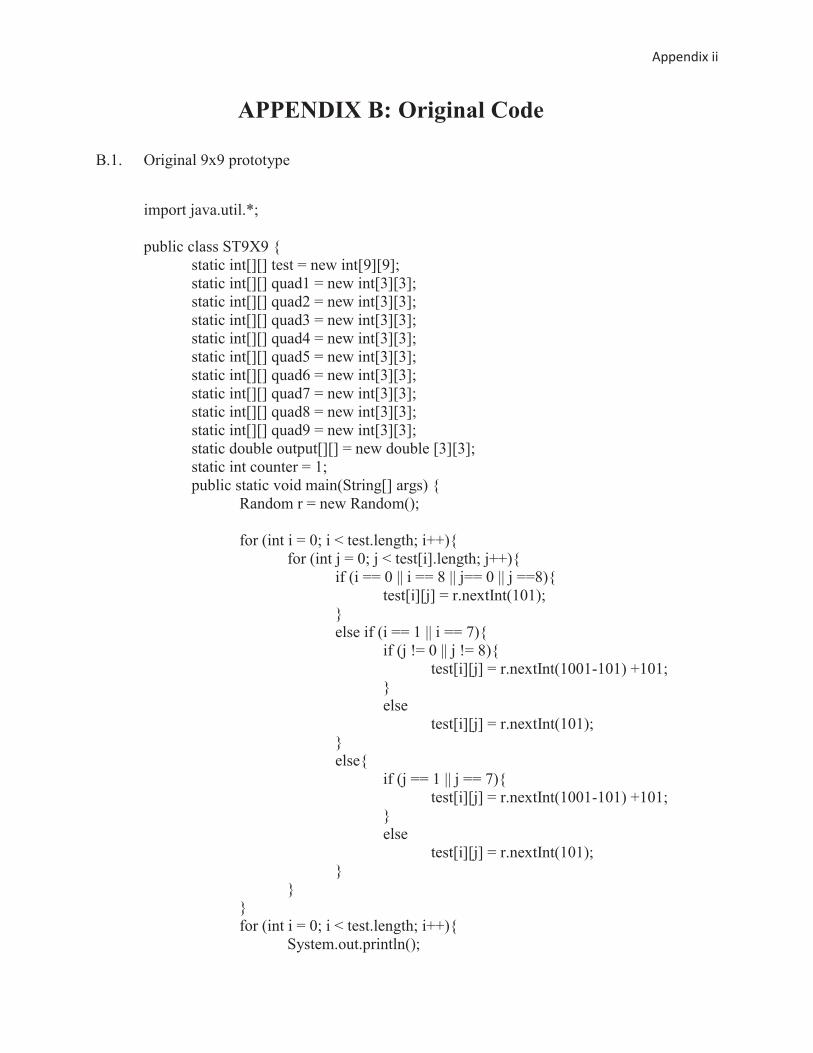
Appendix ii
APPENDIX B: Original Code
B.1. Original 9x9 prototype
import java.util.*; public class ST9X9 { static int[][] test = new int[9][9]; static int[][] quad1 = new int[3][3]; static int[][] quad2 = new int[3][3]; static int[][] quad3 = new int[3][3]; static int[][] quad4 = new int[3][3]; static int[][] quad5 = new int[3][3]; static int[][] quad6 = new int[3][3]; static int[][] quad7 = new int[3][3]; static int[][] quad8 = new int[3][3]; static int[][] quad9 = new int[3][3]; static double output[][] = new double [3][3]; static int counter = 1; public static void main(String[] args) { Random r = new Random(); for (int i = 0; i < test.length; i++){ for (int j = 0; j < test[i].length; j++){ if (i == 0 || i == 8 || j== 0 || j ==8){ test[i][j] = r.nextInt(101); } else if (i == 1 || i == 7){ if (j != 0 || j != 8){ test[i][j] = r.nextInt(1001-101) +101; } else test[i][j] = r.nextInt(101); } else{ if (j == 1 || j == 7){ test[i][j] = r.nextInt(1001-101) +101; } else test[i][j] = r.nextInt(101); } } } for (int i = 0; i < test.length; i++){ System.out.println();
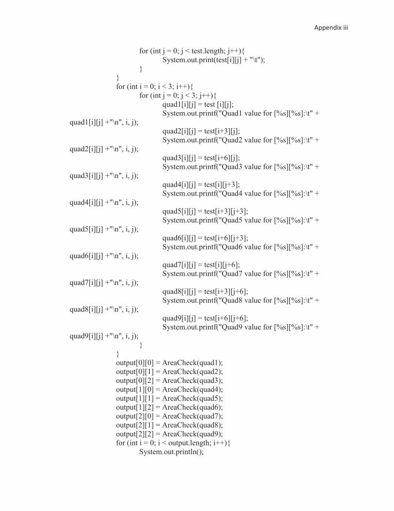
Appendix iii
for (int j = 0; j < test.length; j++){ System.out.print(test[i][j] + "\t"); } } for (int i = 0; i < 3; i++){ for (int j = 0; j < 3; j++){ quad1[i][j] = test [i][j]; System.out.printf("Quad1 value for [%s][%s]:\t" + quad1[i][j] +"\n", i, j); quad2[i][j] = test[i+3][j]; System.out.printf("Quad2 value for [%s][%s]:\t" + quad2[i][j] +"\n", i, j); quad3[i][j] = test[i+6][j]; System.out.printf("Quad3 value for [%s][%s]:\t" + quad3[i][j] +"\n", i, j); quad4[i][j] = test[i][j+3]; System.out.printf("Quad4 value for [%s][%s]:\t" + quad4[i][j] +"\n", i, j); quad5[i][j] = test[i+3][j+3]; System.out.printf("Quad5 value for [%s][%s]:\t" + quad5[i][j] +"\n", i, j); quad6[i][j] = test[i+6][j+3]; System.out.printf("Quad6 value for [%s][%s]:\t" + quad6[i][j] +"\n", i, j); quad7[i][j] = test[i][j+6]; System.out.printf("Quad7 value for [%s][%s]:\t" + quad7[i][j] +"\n", i, j); quad8[i][j] = test[i+3][j+6]; System.out.printf("Quad8 value for [%s][%s]:\t" + quad8[i][j] +"\n", i, j); quad9[i][j] = test[i+6][j+6]; System.out.printf("Quad9 value for [%s][%s]:\t" + quad9[i][j] +"\n", i, j); } } output[0][0] = AreaCheck(quad1); output[0][1] = AreaCheck(quad2); output[0][2] = AreaCheck(quad3); output[1][0] = AreaCheck(quad4); output[1][1] = AreaCheck(quad5); output[1][2] = AreaCheck(quad6); output[2][0] = AreaCheck(quad7); output[2][1] = AreaCheck(quad8); output[2][2] = AreaCheck(quad9); for (int i = 0; i < output.length; i++){ System.out.println();
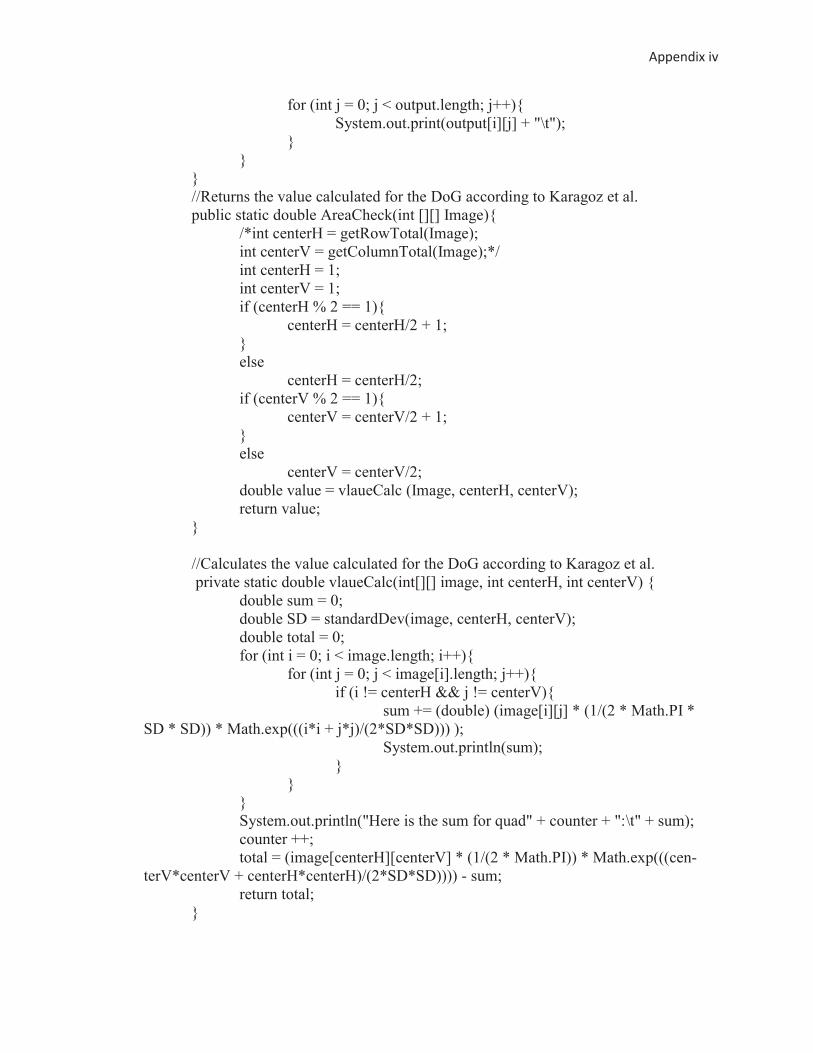
Appendix iv
for (int j = 0; j < output.length; j++){ System.out.print(output[i][j] + "\t"); } } } //Returns the value calculated for the DoG according to Karagoz et al. public static double AreaCheck(int [][] Image){ /*int centerH = getRowTotal(Image); int centerV = getColumnTotal(Image);*/ int centerH = 1; int centerV = 1; if (centerH % 2 == 1){ centerH = centerH/2 + 1; } else centerH = centerH/2; if (centerV % 2 == 1){ centerV = centerV/2 + 1; } else centerV = centerV/2; double value = vlaueCalc (Image, centerH, centerV); return value; } //Calculates the value calculated for the DoG according to Karagoz et al. private static double vlaueCalc(int[][] image, int centerH, int centerV) { double sum = 0; double SD = standardDev(image, centerH, centerV); double total = 0; for (int i = 0; i < image.length; i++){ for (int j = 0; j < image[i].length; j++){ if (i != centerH && j != centerV){ sum += (double) (image[i][j] * (1/(2 * Math.PI * SD * SD)) * Math.exp(((i*i + j*j)/(2*SD*SD))) ); System.out.println(sum); } } } System.out.println("Here is the sum for quad" + counter + ":\t" + sum); counter ++; total = (image[centerH][centerV] * (1/(2 * Math.PI)) * Math.exp(((cen-terV*centerV + centerH*centerH)/(2*SD*SD)))) - sum; return total; }
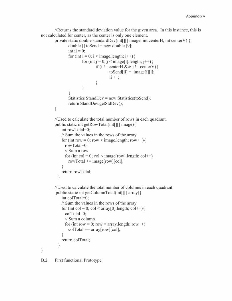
Appendix v
//Returns the standard deviation value for the given area. In this instance, this is not calculated for center, as the center is only one element. private static double standardDev(int[][] image, int centerH, int centerV) { double [] toSend = new double [9]; int ii = 0; for (int i = 0; i < image.length; i++){ for (int j = 0; j < image[i].length; j++){ if (i != centerH && j != centerV){ toSend[ii] = image[i][j]; ii ++; } } } Statistics StandDev = new Statistics(toSend); return StandDev.getStdDev(); } //Used to calculate the total number of rows in each quadrant. public static int getRowTotal(int[][] image){ int rowTotal=0; // Sum the values in the rows of the array for (int row = 0; row < image.length; row++){ rowTotal=0; // Sum a row for (int col = 0; col < image[row].length; col++) rowTotal += image[row][col]; } return rowTotal; } //Used to calculate the total number of columns in each quadrant. public static int getColumnTotal(int[][] array){ int colTotal=0; // Sum the values in the rows of the array for (int col = 0; col < array[0].length; col++){ colTotal=0; // Sum a column for (int row = 0; row < array.length; row++) colTotal += array[row][col]; } return colTotal; } }
B.2. First functional Prototype
Appendix vi
import java.awt.image.BufferedImage; import java.io.File; import java.io.IOException; import javax.imageio.ImageIO; public class ST_Filter { static File file = new File( "C:\\Users\\Jon Gesell\\Google Drive\\Thesis\\ST Fil-ter\\lena512_8bit.bmp"); static int width = 0; static int height = 0; static int Vt = 10; static int Tau = 5; static int R = 10; static int Vr = -65; static double nt = -0.1; static int spkthr = -50; static BufferedImage originalImage = null; static int Ac = 3; static int As = 1; static double sigmaC = 0; static double sigmaS = 0; static double min = Integer.MAX_VALUE; static double max = 0; static int Radius = 7; static int horizontalFilters = 16; static int verticalFilters = 16; public static void main (String args[]) throws IOException{ try { originalImage = ImageIO.read(file); } catch (IOException e) { System.out.println("No such image exists"); } width = originalImage.getWidth(); height = originalImage.getHeight(); double [][] imageQuad1 = new double [height/2][width/2]; double [][] imageQuad2 = new double [height/2][width/2]; double [][] imageQuad3 = new double [height/2][width/2]; double [][] imageQuad4 = new double [height/2][width/2]; double [][] image = new double [height][width]; System.out.println("Width = " + width + "\nHeight = " + height); for (int y = 0; y < height/2 ; y++){ for (int x = 0; x < width/2; x++){ imageQuad1 [x][y] = originalImage.getRGB(x,y); imageQuad2 [x][y] = originalImage.getRGB(x + width/2, y);
Appendix vii
imageQuad3 [x][y] = originalImage.getRGB(x, y + height/2); imageQuad4 [x][y] = originalImage.getRGB(x + width/2, y + height/2); } } double[][] normalizedQuad1 = Normalize(imageQuad1); double[][] normalizedQuad2 = Normalize(imageQuad2); double[][] normalizedQuad3 = Normalize(imageQuad3); double[][] normalizedQuad4 = Normalize(imageQuad4); sigmaC = sigmaC/4; imageQuad1 = MatrixCreate(normalizedQuad1, Radius); imageQuad2 = MatrixCreate(normalizedQuad2, Radius); imageQuad3 = MatrixCreate(normalizedQuad3, Radius); imageQuad4 = MatrixCreate(normalizedQuad4, Radius); for (int y = 0; y < height/2 ; y++){ for (int x = 0; x < width/2; x++){ image[x][y] = imageQuad1[x][y] * origi-nalImage.getRGB(x, y); image[x + width/2][y] = imageQuad2[x][y] * origi-nalImage.getRGB(x + width/2, y); image[x][y + height/2] = imageQuad3[x][y] * origi-nalImage.getRGB(x, y + height/2); image[x + width/2][y + height/2] = imageQuad4[x][y] * originalImage.getRGB(x + width/2, y + height/2); } } Radius = 4; Ac = 2; System.out.println("Width = " + width + "\nHeight = " + height); for (int y = 0; y < height/2 ; y++){ for (int x = 0; x < width/2; x++){ imageQuad1 [x][y] = image[x][y]; imageQuad2 [x][y] = image[x + width/2][y]; imageQuad3 [x][y] = image[x][y + height/2]; imageQuad4 [x][y] = image[x + width/2][y + height/2]; } } normalizedQuad1 = Normalize(imageQuad1); normalizedQuad2 = Normalize(imageQuad2); normalizedQuad3 = Normalize(imageQuad3); normalizedQuad4 = Normalize(imageQuad4); sigmaC = sigmaC/4; imageQuad1 = MatrixCreate(normalizedQuad1, Radius); imageQuad2 = MatrixCreate(normalizedQuad2, Radius); imageQuad3 = MatrixCreate(normalizedQuad3, Radius);
Appendix viii
imageQuad4 = MatrixCreate(normalizedQuad4, Radius); for (int y = 0; y < height/2 ; y++){ for (int x = 0; x < width/2; x++){ image[x][y] = imageQuad1[x][y] * origi-nalImage.getRGB(x, y); image[x + width/2][y] = imageQuad2[x][y] * origi-nalImage.getRGB(x + width/2, y); image[x][y + height/2] = imageQuad3[x][y] * origi-nalImage.getRGB(x, y + height/2); image[x + width/2][y + height/2] = imageQuad4[x][y] * originalImage.getRGB(x + width/2, y + height/2); } } BufferedImage imageOut = new BufferedImage (width, height, Buff-eredImage.TYPE_4BYTE_ABGR); for(int y = 0; y < height; y++){ for(int x = 0; x < width; x++){ imageOut.setRGB(x, y, (int)Math.round(image[x][y])); } } File imageFile = new File("C:\\Users\\Jon Gesell\\Google Drive\\The-sis\\ST Filter\\imageOut_V5.bmp"); ImageIO.write(imageOut, "bmp", imageFile); System.out.println("New image located at \'C:\\Users\\Jon Gesell\\Google Drive\\Thesis\\ST Filter\\imageOut_V4.bmp\'"); } private static double STFB(int Ac, int As, double sigmaC, double sigmaS, int x, int y, double PixelIn){ double PixelOut = PixelIn * (Ac * (Math.exp(-1*(x^2 + y^2))/(2*Math.PI*sigmaC)) - (As * (Math.exp(-1*(x^2 + y^2))/(2*Math.PI*sigmaS)))); return PixelOut; } private static double[][] MatrixCreate(double [][] imageIn, int Radius){ int Center = Radius/2 + 1; double[][] matrixX = new double[imageIn.length][imageIn[0].length]; double[][] matrixY = new double[imageIn.length][imageIn[0].length]; double[][] matrixOut = new double[imageIn.length][imageIn[0].length]; for (int y = imageIn.length - 1; y >= 0; y--){ for (int x = imageIn.length - 1; x >=0; x--){ if (x != Center && y != Center){ matrixX[x][y] = 0; matrixY[x][y] = 0; } else if (x == Center && y != Center){
Appendix ix
matrixX[x][y] = STFB(Ac, As, sigmaC, sigmaS, Math.abs(Center - x), Math.abs(Center - y), imageIn[Math.abs(x - Radius)][Math.abs(y - Radius)]); matrixY[x][y] = 0; } else if (x != Center && y == Center){ matrixX[x][y] = 0; matrixY[x][y] = STFB(Ac, As, sigmaC, sigmaS, Math.abs(Center - x), Math.abs(Center - y), imageIn[Math.abs(x - Radius)][Math.abs(y - Radius)]); } else if (x == Center && y == Center){ matrixX[x][y] = STFB(Ac, As, sigmaC, sigmaS, Math.abs(Center - x), Math.abs(Center - y), imageIn[Math.abs(x - Radius)][Math.abs(y - Radius)]); matrixY[x][y] = STFB(Ac, As, sigmaC, sigmaS, Math.abs(Center - x), Math.abs(Center - y), imageIn[Math.abs(x - Radius)][Math.abs(y - Radius)]); } } } matrixOut = MatrixMultiply (matrixX, matrixY); return matrixOut; } private static double[][] MatrixMultiply(double[][] matrixX, double[][] matrixY) { double [][] matrixOut = new double [matrixX.length][matrixX.length]; for (int y = 0; y < matrixOut.length; y++){ for (int x = 0; x < matrixOut.length; x ++){ for (int z = 0; z < matrixOut.length; z++){ matrixOut[x][y] = matrixX[x][z] * matrixY[z][y]; } } } return matrixOut; } private static double NLIF(double PixelIn){ double SpikeOut = 0; int I = 600; int t0 = 0; int vthreshold = 15; int vr = 0; int tauM = 10; int vt = 0; int t = vt = vr*Math.exp(arg0)
Appendix x
return SpikeOut; } private static double[][] Normalize (double [][] imageIn){ double imageOut[][] = new double[imageIn.length][imageIn[0].length]; for (int a = 0; a < imageIn.length; a ++){ for (int b = 0; b < imageIn[0].length; b++){ imageOut[b][a] = (imageIn[b][a] - min)/(max - min); } } StandardDeviation(imageOut); return imageOut; } private static void StandardDeviation(double[][] normalized) { double average = 0; for (int a = 0; a < normalized.length; a ++){ for (int b = 0; b < normalized[0].length; b++){ average += normalized[b][a]; } } average = Math.sqrt(average/(normalized[0].length * normalized.length)); for (int a = 0; a < normalized.length; a ++){ for (int b = 0; b < normalized[0].length; b++){ normalized[b][a] = normalized[b][a] - average; normalized[b][a] = normalized[b][a] * normalized[b][a]; } } average = 0; for (int a = 0; a < normalized.length; a ++){ for (int b = 0; b < normalized[0].length; b++){ average += normalized[b][a]; } } sigmaC += Math.sqrt(average/(normalized[0].length * normal-ized.length)); } }
B.3. Second Functional Prototype
import java.awt.*; import java.awt.image.BufferedImage; import java.io.*; import java.util.*; import javax.imageio.ImageIO; public class STFilter {
Appendix xi
static File file = new File( "./lena512_8bit.bmp"); static BufferedImage originalImage = null; static int counter = 0; static int centerH = 0; static int centerV = 0; static int min = 0; static int max = 0; static double thetaC = 0; static double thetaS = 0; static int width = 0; static int height = 0; static int Ac = 3; static int As = 1; public static void main (String args[]) throws IOException{ try { originalImage = ImageIO.read(file); } catch (IOException e) { System.out.println("No such image exists"); } width = originalImage.getWidth(); height = originalImage.getHeight(); double [][] finalOut = new double [width][height]; int [][] Image = new int[width][height]; double [][] normalized = new double[width][height]; for (int a = 0; a < height; a ++){ //System.out.println(); for (int b = 0; b < width; b++){ finalOut[b][a] = 0; Image[b][a] = originalImage.getRGB(b, a); //System.out.print("\t" + Image[b][a]); if (min > -1 * originalImage.getRGB(b,a)){ min = originalImage.getRGB(b, a); } if (max < -1 * originalImage.getRGB(b,a)){ max = originalImage.getRGB(b, a); } } } System.out.println ("Max: "+ max + "\t Min: "+min); for (int a = 0; a < height; a ++){ //System.out.println(); for (int b = 0; b < width; b++){ normalized[b][a] = (Image[b][a] - min)/(max - min); //System.out.print("\t" + normalized[b][a]); } }
Appendix xii
thetaC = StandardDeviation(normalized); System.out.println("Theta C: " + thetaC); thetaS = thetaC * 6; System.out.println("Theta S: " + thetaS); for (centerV = height/16; centerV < height; centerV += height/16){ for (centerH = width/16; centerH < width; centerH += width/16){ finalOut = FilterFirst(normalized, finalOut); counter ++; } } System.out.println("Number of ST Filters used: " + counter); for (int a = 0; a < height; a ++){ //System.out.println(); for (int b = 0; b < width; b++){ finalOut[b][a] = finalOut[b][a]/counter; //System.out.println(counter); //System.out.print("\t" + finalOut[b][a]); } } BufferedImage imageOut = new BufferedImage (width, height, Buff-eredImage.TYPE_BYTE_GRAY); for(int y = 0; y < height; y++){ for(int x = 0; x < width; x++){ imageOut.setRGB(x, y, (int)Math.round(finalOut[x][y])); } } File imageFile = new File("./imageOut.bmp"); ImageIO.write(imageOut, "bmp", imageFile); System.out.println("New image located at \'./imageOut.bmp\'"); } private static double[][] FilterFirst(double[][] normalized, double[][] finalOut) { for (int a = 0; a < height; a ++){ int y = centerV - a; int maximum = 256^4; //System.out.println(); for (int b = 0; b < width; b++){ int x = centerH - b; finalOut[b][a] += ((Ac/(2*Math.PI*thetaC*thetaC))*(Math.exp((x^2 + y^2)/(2*thetaC*thetaC))) - (As/(2*Math.PI*thetaS*thetaS))*Math.exp((x^2+y^2)/(2*thetaS*thetaS))) * normal-ized[b][a]; if(finalOut[b][a] >= maximum) finalOut[b][a] = -1*maximum - 1; //System.out.print("\t" + finalOut[b][a]);
Appendix xiii
} } return finalOut; } private static double StandardDeviation(double[][] normalized) { double average = 0; for (int a = 0; a < height; a ++){ for (int b = 0; b < width; b++){ average += normalized[b][a]; } } average = Math.sqrt(average/(width * height)); for (int a = 0; a < height; a ++){ for (int b = 0; b < width; b++){ normalized[b][a] = normalized[b][a] - average; normalized[b][a] = normalized[b][a] * normalized[b][a]; } } average = 0; for (int a = 0; a < height; a ++){ for (int b = 0; b < width; b++){ average += normalized[b][a]; } } average = Math.sqrt(average/(width * height)); return average; } }
Appendix xiv
APPENDIX C: Original Radius Code
C.1. Original Version
import java.awt.*; import java.awt.image.BufferedImage; import java.io.*; import java.util.*; import javax.imageio.ImageIO; public class STFilterRadius { static File file = new File( "C:\\Users\\Jon Gesell\\workspace\\The-sis\\src\\lena512_8bit.bmp"); static BufferedImage originalImage = null; static int counter = 0; static int centerH = 0; static int centerV = 0; static double min = Integer.MAX_VALUE; static double max = 0; static double thetaC = 0; static double thetaS = 0; static int width = 0; static int height = 0; static int Ac = 3; static int As = 1; static int horizontalFilters = 16; static int verticalFilters = 16; static int yRad = 0; static int xRad = 0; public static void main (String args[]) throws IOException{ Scanner input = new Scanner(System.in); try { originalImage = ImageIO.read(file); } catch (IOException e) { System.out.println("No such image exists"); } System.out.print("Please enter the number of horizontal filters to be used (best result: at least 16):\t"); horizontalFilters = input.nextInt(); System.out.print("Please enter the number of vertical filters to be used (best result: at least 16):\t"); verticalFilters = input.nextInt(); long startTime = System.currentTimeMillis(); width = originalImage.getWidth();
Appendix xv
height = originalImage.getHeight(); double [][] finalOut = new double [width][height]; double[][] Image = new double[width][height]; double [][] normalized = new double[width][height]; for (int a = 0; a < height; a ++){ //System.out.println(); for (int b = 0; b < width; b++){ finalOut[b][a] = 0; Image[b][a] = originalImage.getRGB(b, a); //System.out.print("\t" + Image[b][a]); } } imageProcess(Image); normalized = normalize(Image); // System.out.println ("Max: "+ max + "\t Min: "+min); thetaC = StandardDeviation(normalized); // System.out.println("Theta C: " + thetaC); thetaS = thetaC * 6; //System.out.println("Theta S: " + thetaS); yRad = height/verticalFilters; xRad = width/horizontalFilters; for (int vert = Math.round(height/verticalFilters); vert <= height; vert += height/verticalFilters){ centerV = vert - (height/verticalFilters)/2; for (int hor = Math.round(width/horizontalFilters); hor <= width; hor += width/horizontalFilters){ centerH = hor - (width/horizontalFilters)/2; finalOut = Filter(normalized, finalOut); counter ++; } } // System.out.println("Number of ST Filters used: " + counter); for (int a = 0; a < height; a ++){ //System.out.println(); for (int b = 0; b < width; b++){ finalOut[b][a] = finalOut[b][a]/counter; finalOut[b][a] = finalOut[b][a] * 256*256*256*256; //System.out.println(counter); //System.out.print("\t" + finalOut[b][a]); } } counter = 0; Ac = 2; imageProcess(finalOut); // System.out.println ("Max: "+ max + "\t Min: "+min);
Appendix xvi
normalized = normalize(finalOut); thetaC = StandardDeviation(normalized); // System.out.println("Theta C: " + thetaC); thetaS = thetaC * 6; // System.out.println("Theta S: " + thetaS); for (int vert = Math.round(height/verticalFilters); vert <= height; vert += height/verticalFilters){ centerV = vert - (height/verticalFilters)/2; for (int hor = Math.round(width/horizontalFilters); hor <= width; hor += width/horizontalFilters){ centerH = hor - (width/horizontalFilters)/2; finalOut = Filter(normalized, finalOut); counter ++; } } // System.out.println("Number of ST Filters used: " + counter); /* for (int a = 0; a < height; a ++){ //System.out.println(); for (int b = 0; b < width; b++){ finalOut[b][a] = finalOut[b][a]/counter; finalOut[b][a] = finalOut[b][a] * 256*256*256*256; //System.out.println(counter); //System.out.print("\t" + finalOut[b][a]); } }*/ BufferedImage imageOut = new BufferedImage (width, height, Buff-eredImage.TYPE_BYTE_GRAY); for(int y = 0; y < height; y++){ for(int x = 0; x < width; x++){ imageOut.setRGB(x, y, (int)Math.round(finalOut[x][y])); } } File imageFile = new File("C:\\Users\\Jon Gesell\\workspace\\The-sis\\src\\imageOut with Radius16.bmp"); ImageIO.write(imageOut, "bmp", imageFile); System.out.println("New image located at \'C:\\Users\\Jon Gesell\\work-space\\Thesis\\src\\imageOut with Radius.bmp\'"); long endTime = System.currentTimeMillis(); long totalTime = endTime - startTime; System.out.println(totalTime); } private static double[][] normalize(double[][] image) { double [][] normalize = new double [width][height]; for (int a = 0; a < height; a ++){
Appendix xvii
//System.out.println(); for (int b = 0; b < width; b++){ normalize[b][a] = (image[b][a] - min)/(max - min); //System.out.print("\t" + normalized[b][a]); } } return normalize; } private static void imageProcess(double[][] image) { for (int a = 0; a < height; a ++){ //System.out.println(); for (int b = 0; b < width; b++){ if (min > Math.abs(image[b][a])){ min = image[b][a]; } if (max < Math.abs(image[b][a])){ max = image[b][a]; } } } } private static double[][] Filter(double[][] normalized, double[][] finalOut) { for (int a = 0; a < height; a ++){ int y = Math.abs(centerV - a); //int maximum = 256^4; if (Math.abs(y) <= yRad){ //System.out.println(); for (int b = 0; b < width; b++){ int x = Math.abs(centerH - b); if (Math.abs(x) <= xRad){ finalOut[b][a] += ((Ac/(2*Math.PI*thetaC*thetaC))*(Math.exp(-1* (x^2 + y^2)/(2*thetaC*thetaC))) - (As/(2*Math.PI*thetaS*thetaS))*Math.exp(-1*(x^2+y^2)/(2*thetaS*thetaS))) * normal-ized[b][a]; /*if(finalOut[b][a] >= maximum) finalOut[b][a] = -1*maximum - 1;*/ //System.out.print("\t" + finalOut[b][a]); } } } } return finalOut; } private static double StandardDeviation(double[][] normalized) {
Appendix xviii
double average = 0; for (int a = 0; a < height; a ++){ for (int b = 0; b < width; b++){ average += normalized[b][a]; } } average = Math.sqrt(average/(width * height)); for (int a = 0; a < height; a ++){ for (int b = 0; b < width; b++){ normalized[b][a] = normalized[b][a] - average; normalized[b][a] = normalized[b][a] * normalized[b][a]; } } average = 0; for (int a = 0; a < height; a ++){ for (int b = 0; b < width; b++){ average += normalized[b][a]; } } average = Math.sqrt(average/(width * height)); return average; } }
C.2. Updated Version
import java.awt.*; import java.awt.image.BufferedImage; import java.io.*; import java.util.*; import javax.imageio.ImageIO; public class STFilterRadius { static File file = new File( "C:\\Users\\Jon Gesell\\workspace\\The-sis\\src\\lena512_8bit.bmp"); static BufferedImage originalImage = null; static int counter = 0; static int centerH = 0; static int centerV = 0; static double min = Integer.MAX_VALUE; static double max = 0; static double thetaC = 0; static double thetaS = 0; static int width = 0; static int height = 0;
Appendix xix
static int Ac = 3; static int As = 1; static int horizontalFilters = 16; static int verticalFilters = 16; static int yRad = 0; static int xRad = 0; public static void main (String args[]) throws IOException{ Scanner input = new Scanner(System.in); try { originalImage = ImageIO.read(file); } catch (IOException e) { System.out.println("No such image exists"); } System.out.print("Please enter the number of horizontal filters to be used (best result: at least 16):\t"); horizontalFilters = input.nextInt(); System.out.print("Please enter the number of vertical filters to be used (best result: at least 16):\t"); verticalFilters = input.nextInt(); long startTime = System.currentTimeMillis(); width = originalImage.getWidth(); height = originalImage.getHeight(); double [][] finalOut = new double [width][height]; double[][] Image = new double[width][height]; double [][] normalized = new double[width][height]; for (int a = 0; a < height; a ++){ //System.out.println(); for (int b = 0; b < width; b++){ finalOut[b][a] = 0; Image[b][a] = originalImage.getRGB(b, a); //System.out.print("\t" + Image[b][a]); } } imageProcess(Image); normalized = normalize(Image); // System.out.println ("Max: "+ max + "\t Min: "+min); thetaC = StandardDeviation(normalized); // System.out.println("Theta C: " + thetaC); thetaS = thetaC * 6; //System.out.println("Theta S: " + thetaS); yRad = height/verticalFilters; xRad = width/horizontalFilters; for (int vert = Math.round(height/verticalFilters); vert <= height; vert += height/verticalFilters){ centerV = vert - (height/verticalFilters)/2;
Appendix xx
for (int hor = Math.round(width/horizontalFilters); hor <= width; hor += width/horizontalFilters){ centerH = hor - (width/horizontalFilters)/2; finalOut = Filter(normalized, finalOut); counter ++; } } // System.out.println("Number of ST Filters used: " + counter); for (int a = 0; a < height; a ++){ //System.out.println(); for (int b = 0; b < width; b++){ finalOut[b][a] = finalOut[b][a]/counter; finalOut[b][a] = finalOut[b][a] * 256*256*256*256; //System.out.println(counter); //System.out.print("\t" + finalOut[b][a]); } } counter = 0; Ac = 2; imageProcess(finalOut); // System.out.println ("Max: "+ max + "\t Min: "+min); normalized = normalize(finalOut); thetaC = StandardDeviation(normalized); // System.out.println("Theta C: " + thetaC); thetaS = thetaC * 6; // System.out.println("Theta S: " + thetaS); for (int vert = Math.round(height/verticalFilters); vert <= height; vert += height/verticalFilters){ centerV = vert - (height/verticalFilters)/2; for (int hor = Math.round(width/horizontalFilters); hor <= width; hor += width/horizontalFilters){ centerH = hor - (width/horizontalFilters)/2; finalOut = Filter(normalized, finalOut); counter ++; } } // System.out.println("Number of ST Filters used: " + counter); /* for (int a = 0; a < height; a ++){ //System.out.println(); for (int b = 0; b < width; b++){ finalOut[b][a] = finalOut[b][a]/counter; finalOut[b][a] = finalOut[b][a] * 256*256*256*256; //System.out.println(counter); //System.out.print("\t" + finalOut[b][a]); }
Appendix xxi
}*/ BufferedImage imageOut = new BufferedImage (width, height, Buff-eredImage.TYPE_BYTE_GRAY); for(int y = 0; y < height; y++){ for(int x = 0; x < width; x++){ imageOut.setRGB(x, y, (int)Math.round(finalOut[x][y])); } } File imageFile = new File("C:\\Users\\Jon Gesell\\workspace\\The-sis\\src\\imageOut with Radius16.bmp"); ImageIO.write(imageOut, "bmp", imageFile); System.out.println("New image located at \'C:\\Users\\Jon Gesell\\work-space\\Thesis\\src\\imageOut with Radius.bmp\'"); long endTime = System.currentTimeMillis(); long totalTime = endTime - startTime; System.out.println(totalTime); } private static double[][] normalize(double[][] image) { double [][] normalize = new double [width][height]; for (int a = 0; a < height; a ++){ //System.out.println(); for (int b = 0; b < width; b++){ normalize[b][a] = (image[b][a] - min)/(max - min); //System.out.print("\t" + normalized[b][a]); } } return normalize; } private static void imageProcess(double[][] image) { for (int a = 0; a < height; a ++){ //System.out.println(); for (int b = 0; b < width; b++){ if (min > Math.abs(image[b][a])){ min = image[b][a]; } if (max < Math.abs(image[b][a])){ max = image[b][a]; } } } } private static double[][] Filter(double[][] normalized, double[][] finalOut) { for (int a = 0; a < height; a ++){
Appendix xxii
int y = Math.abs(centerV - a); //int maximum = 256^4; if (Math.abs(y) <= yRad){ //System.out.println(); for (int b = 0; b < width; b++){ int x = Math.abs(centerH - b); if (Math.abs(x) <= xRad){ finalOut[b][a] += ((Ac/(2*Math.PI*thetaC*thetaC))*(Math.exp(-1* (x^2 + y^2)/(2*thetaC*thetaC))) - (As/(2*Math.PI*thetaS*thetaS))*Math.exp(-1*(x^2+y^2)/(2*thetaS*thetaS))) * normal-ized[b][a]; /*if(finalOut[b][a] >= maximum) finalOut[b][a] = -1*maximum - 1;*/ //System.out.print("\t" + finalOut[b][a]); } } } } return finalOut; } private static double StandardDeviation(double[][] normalized) { double average = 0; for (int a = 0; a < height; a ++){ for (int b = 0; b < width; b++){ average += normalized[b][a]; } } average = Math.sqrt(average/(width * height)); for (int a = 0; a < height; a ++){ for (int b = 0; b < width; b++){ normalized[b][a] = normalized[b][a] - average; normalized[b][a] = normalized[b][a] * normalized[b][a]; } } average = 0; for (int a = 0; a < height; a ++){ for (int b = 0; b < width; b++){ average += normalized[b][a]; } } average = Math.sqrt(average/(width * height)); return average; } }
Appendix xxiii
APPENDIX D: Original Multicore code
import java.awt.Image; import java.awt.List; import java.awt.image.BufferedImage; import java.io.BufferedReader; import java.io.File; import java.io.FileReader; import java.io.IOException; import java.util.ArrayList; import java.util.concurrent.ExecutorService; import java.util.concurrent.Executors; import javax.imageio.ImageIO; public class ST_Test_V2_Multi { static ExecutorService threadPool = Executors.newFixedThreadPool(6); static File previous = new File ("C:\\Users\\Jon\\Google Drive\\Thesis\\ST Fil-ter\\Workbench\\Thesis 2013\\src\\1.bmp"); static File current = new File ("C:\\Users\\Jon\\Google Drive\\Thesis\\ST Fil-ter\\Workbench\\Thesis 2013\\src\\1.bmp"); static File next = new File ("C:\\Users\\Jon\\Google Drive\\Thesis\\ST Fil-ter\\Workbench\\Thesis 2013\\src\\1.bmp"); static ImageData prev1; static ImageData curr1; static ImageData next1; static BufferedImage prevImg; static BufferedImage currImg; static BufferedImage nextImg; static ImageData inter1; static ImageData inter2; static ImageData curr2; static ImageData prev2; static BufferedImage interIm1; static BufferedImage interIm2; static double [][] STOut11; static double [][] STOut12; static double [][] STOut21; static BufferedImage imageOut; static int threads = 0; public static void main(String[] args) throws IOException { try { prevImg = ImageIO.read(previous); currImg = ImageIO.read(current); nextImg = ImageIO.read(next);
Appendix xxiv
prev1 = new ImageData (prevImg, 3); curr1 = new ImageData (currImg, 3); next1 = new ImageData (nextImg, 3); } catch (IOException e1) { System.out.println("Image files missing"); e1.printStackTrace(); } STOut11 = new double [prev1.height][prev1.width]; STOut12 = new double [curr1.height][curr1.width]; for (threads = 0; threads < 4; threads ++){ threadPool.submit(new Runnable(){ public void run() { for (int height = 0; height < prev1.height/2; height ++){ for (int width = 0; width < prev1.width/2; width ++){ STOut11 [height][width] = (curr1.centerGaussian1[height][width] - prev1.surroundGaussian [height][width]); STOut11 [height + prev1.height/2][width] = (curr1.centerGaussian1[height + prev1.height/2][width] - prev1.surroundGaussian [height + prev1.height/2][width]); STOut11 [height][width + prev1.width/2] = (curr1.centerGaussian1[height][width + prev1.width/2] - prev1.sur-roundGaussian [height][width + prev1.width/2]); STOut11 [height + prev1.height/2][width + prev1.width/2] = (curr1.centerGaussian1[height + prev1.height/2][width + prev1.width/2] - prev1.surroundGaussian [height + prev1.height/2][width + prev1.width/2]); STOut12 [height][width] = (prev1.centerGaussian1[height][width] - curr1.surroundGaussian [height][width]); STOut12 [height + prev1.height/2][width] = (prev1.centerGaussian1[height + prev1.height/2][width] - curr1.surroundGaussian [height + prev1.height/2][width]); STOut12 [height][width + prev1.width/2] = (prev1.centerGaussian1[height][width + prev1.width/2] - curr1.sur-roundGaussian [height][width + prev1.width/2]); STOut12 [height + prev1.height/2][width + prev1.width/2] = (prev1.centerGaussian1[height + prev1.height/2][width + prev1.width/2] - curr1.surroundGaussian [height + prev1.height/2][width + prev1.width/2]); } } }}); }
Appendix xxv
interIm1 = new BufferedImage (STOut11.length, STOut11[0].length, BufferedImage.TYPE_BYTE_GRAY); interIm2 = new BufferedImage (STOut12.length, STOut12[0].length, BufferedImage.TYPE_BYTE_GRAY); PartTwo(); } public static void PartTwo(){ for (threads = 0; threads < 4; threads ++){ threadPool.submit(new Runnable() { public void run() { for(int y = 0; y < STOut11.length/2; y++){ for(int x = 0; x < STOut11[0].length/2; x++){ interIm1.setRGB(x, y, (int)Math.round(STOut11[y][x] * 256 * 256 * 256 *256)); interIm1.setRGB(x + STOut11[0].length/2, y, (int)Math.round(STOut11[y][x + STOut11[0].length/2] * 256 * 256 * 256 *256)); interIm1.setRGB(x, y + STOut11.length/2, (int)Math.round(STOut11[y + STOut11.length/2][x] * 256 * 256 * 256 *256)); interIm1.setRGB(x + STOut11[0].length/2, y + STOut11.length/2, (int)Math.round(STOut11[y + STOut11.length/2][x + STOut11[0].length/2] * 256 * 256 * 256 *256)); } } for(int y = 0; y < STOut12.length; y++){ for(int x = 0; x < STOut12[0].length; x++){ interIm2.setRGB(x, y, (int)Math.round(STOut11[y][x]* 256 * 256 * 256 *256)); interIm2.setRGB(x + STOut11[0].length/2, y, (int)Math.round(STOut11[y][x + STOut11[0].length/2]* 256 * 256 * 256 *256)); interIm2.setRGB(x, y + STOut11.length/2, (int)Math.round(STOut11[y + STOut11.length/2][x]* 256 * 256 * 256 *256)); interIm2.setRGB(x + STOut11[0].length/2, y + STOut11.length/2, (int)Math.round(STOut11[y + STOut11.length/2][x + STOut11[0].length/2]* 256 * 256 * 256 *256)); } } } }); } try {
Appendix xxvi
File secondIntermediate = new File("C:\\Users\\Jon\\Google Drive\\Thesis\\ST Filter\\Workbench\\Thesis 2013\\src\\Second_Intermediate.bmp"); ImageIO.write(interIm2, "bmp", secondIntermediate); } catch (IOException e) { System.out.println("Unable to create the second intermediate im-age"); e.printStackTrace(); } try { File firstIntermediate = new File("C:\\Users\\Jon\\Google Drive\\Thesis\\ST Filter\\Workbench\\Thesis 2013\\src\\First_Intermediate.bmp"); ImageIO.write(interIm1, "bmp", firstIntermediate); } catch (IOException e) { System.out.println("Unable to create the first intermediate image"); e.printStackTrace(); } System.out.println("First intermediate image located at 'C:\\Us-ers\\Jon\\Google Drive\\Thesis\\ST Filter\\Workbench\\Thesis 2013\\src\\First_Intermedi-ate.bmp'"); System.out.println("Second intermediate image located at 'C:\\Us-ers\\Jon\\Google Drive\\Thesis\\ST Filter\\Workbench\\Thesis 2013\\src\\Second_Inter-mediate.bmp'"); prev2 = new ImageData (interIm1, 2); curr2 = new ImageData (interIm2, 2); PartThree(); } public static void PartThree(){ STOut21 = new double [prevImg.getHeight()][prevImg.getWidth()]; for (threads = 0; threads < 6; threads ++){ threadPool.submit(new Runnable(){ public void run() { for (int height = 0; height < prevImg.getHeight()/2; height ++){ for (int width = 0; width < pre-vImg.getWidth()/2; width ++){ STOut21 [height][width] = (curr2.centerGaussian1[height][width] - prev2.surroundGaussian [height][width]); STOut21 [height][width + pre-vImg.getWidth()/2] = (curr2.centerGaussian1[height][width + prevImg.getWidth()/2] - prev2.surroundGaussian [height][width + prevImg.getWidth()/2]); STOut21 [height + pre-vImg.getHeight()/2][width] = (curr2.centerGaussian1[height + pre-vImg.getHeight()/2][width] - prev2.surroundGaussian [height + pre-vImg.getHeight()/2][width]);
Appendix xxvii
STOut21 [height + pre-vImg.getHeight()/2][width + prevImg.getWidth()/2] = (curr2.centerGaussian1[height + prevImg.getHeight()/2][width + prevImg.getWidth()/2] - prev2.surroundGaussian [height + prevImg.getHeight()/2][width + prevImg.getWidth()/2]); } } } }); } PartFour(); } public static void PartFour(){ imageOut = new BufferedImage (prevImg.getWidth(), pre-vImg.getHeight(), BufferedImage.TYPE_BYTE_GRAY); for (threads = 0; threads < 6; threads ++){ threadPool.submit(new Runnable(){ public void run() { for(int y = 0; y < prevImg.getHeight()/2; y++){ for(int x = 0; x < prevImg.getWidth()/2; x++){ imageOut.setRGB(x, y, (int)Math.round(STOut21[y][x] * 256*256*256*256)); imageOut.setRGB(x + pre-vImg.getWidth()/2, y, (int)Math.round(STOut21[y][x + prevImg.getWidth()/2] * 256*256*256*256)); imageOut.setRGB(x, y + pre-vImg.getHeight()/2, (int)Math.round(STOut21[y + prevImg.getHeight()/2][x] * 256*256*256*256)); imageOut.setRGB(x + pre-vImg.getWidth()/2, y + prevImg.getHeight()/2, (int)Math.round(STOut21[y + pre-vImg.getHeight()/2][x + prevImg.getWidth()/2] * 256*256*256*256)); } } } }); } try { File imageFile = new File("C:\\Users\\Jon\\Google Drive\\The-sis\\ST Filter\\Workbench\\Thesis 2013\\src\\imageOut_V5.bmp"); ImageIO.write(imageOut, "bmp", imageFile); } catch (IOException e) { System.out.println("Failed to create second output image"); e.printStackTrace(); }
Appendix xxviii
System.out.println("New image located at \'C:\\Users\\Jon\\Google Drive\\Thesis\\ST Filter\\Workbench\\Thesis 2013\\src\\imageOut_V5.bmp\'"); } } import java.awt.image.BufferedImage; import java.util.concurrent.ExecutorService; import java.util.concurrent.Executors; public class ImageData_Multicore { static double min = Integer.MAX_VALUE; static double max = Integer.MIN_VALUE; static double sigmaC = 0; static double sigmaS = 0; public int width = 0; public int height = 0; static double [][] centerOut; static double [][] surroundOut; static double[][] normalized; public double [][] centerGaussian1; static double [][] centerGaussian2; public double [][] surroundGaussian; static int Ac = 3; static int As = 1; static double [][] image; static BufferedImage imageIn = null; static ExecutorService threadPool = Executors.newFixedThreadPool(10); static double average = 0; public ImageData_Multicore (BufferedImage imageIn1, int Amp){ imageIn = imageIn1; Ac = Amp; this.width = imageIn.getWidth(); this.height = imageIn.getHeight(); image = new double [height][width]; System.out.println("Height = " + height + " and width = " + width); for (int threads = 0; threads < 4; threads ++){ threadPool.submit(new Runnable(){ public void run() { for (int y = 0; y < height/2; y++){ for (int x = 0; x < width/2; x++){ image[y][x] = imageIn.getRGB(x, y); image[y][x + width/2] = im-ageIn.getRGB(x + width/2, y);
Appendix xxix
image[y + height/2][x] = im-ageIn.getRGB(x, y + height/2); image[y + height/2][x + width/2] = imageIn.getRGB(x + width/2, y + height/2); if (Math.abs(imageIn.getRGB(x, y)) < Math.abs(min)) min = imageIn.getRGB(x, y); if (Math.abs(imageIn.getRGB(x + width/2, y)) < Math.abs(min)) min = imageIn.getRGB(x + width/2, y); if (Math.abs(imageIn.getRGB(x, y + height/2)) < Math.abs(min)) min = imageIn.getRGB(x, y + height/2); if (Math.abs(imageIn.getRGB(x + width/2, y + height/2)) < Math.abs(min)) min = imageIn.getRGB(x + width/2, y + height/2); if (Math.abs(imageIn.getRGB(x, y)) > Math.abs(min)) max = imageIn.getRGB(x, y); if (Math.abs(imageIn.getRGB(x + width/2, y)) > Math.abs(min)) max = imageIn.getRGB(x + width/2, y); if (Math.abs(imageIn.getRGB(x, y + height/2)) > Math.abs(min)) max = imageIn.getRGB(x, y + height/2); if (Math.abs(imageIn.getRGB(x + width/2, y + height/2)) > Math.abs(min)) max = imageIn.getRGB(x + width/2, y + height/2); } } } }); } System.out.println("Image data creation matrix complete, normalizing"); normalized = Normalize (image); this.centerGaussian1 = CenterCalc(normalized); this.surroundGaussian = SurroundCalc(normalized); }
Appendix xxx
private static double[][] Normalize (final double [][] imageIn){ System.out.println("Normalizing of image data starting..."); final double imageOut[][] = new double[imageIn.length][im-ageIn[0].length]; for (int threads = 0; threads < 4; threads ++){ threadPool.submit(new Runnable(){ public void run() { for (int a = 0; a < imageIn.length/2; a ++){ for (int b = 0; b < imageIn[0].length/2; b++){ imageOut[a][b] = (imageIn[a][b] - min)/(max - min); imageOut[a][b + im-ageIn[0].length/2] = (imageIn[a][b + imageIn[0].length/2] - min)/(max - min); imageOut[a + imageIn.length/2][b] = (imageIn[a + imageIn.length/2][b] - min)/(max - min); imageOut[a + imageIn.length/2][b + imageIn[0].length/2] = (imageIn[a + imageIn.length/2][b + imageIn[0].length/2] - min)/(max - min); } } } }); } System.out.println("Normalization of image complete."); StandardDeviation(imageOut); return imageOut; } private static void StandardDeviation(final double[][] normalized) { System.out.println("Finding the standard deviation..."); average = 0; for (int threads = 0; threads < 4; threads ++){ threadPool.submit(new Runnable(){ public void run() { for (int a = 0; a < normalized.length/2; a ++){ for (int b = 0; b < normalized[0].length/2; b++){ average += normalized[a][b]; average += normalized[a][b + nor-malized[0].length/2]; average += normalized[a + normal-ized.length/2][b]; average += normalized[a + normal-ized.length/2][b + normalized[0].length/2]; }
Appendix xxxi
} } }); } average = Math.sqrt(average/(normalized[0].length * normalized.length)); for (int a = 0; a < normalized.length; a ++){ for (int b = 0; b < normalized[0].length; b++){ normalized[a][b] = normalized[a][b] - average; normalized[a][b] = normalized[a][b] * normalized[a][b]; } } average = 0; for (int a = 0; a < normalized.length; a ++){ for (int b = 0; b < normalized[0].length; b++){ average += normalized[a][b]; } } sigmaC += Math.sqrt(average/(normalized[0].length * normal-ized.length)); sigmaS = 6*sigmaC; System.out.println("Data normalization complete, with SigmaC = " + sig-maC + " and SigmaS = " + sigmaS); } private double[][] CenterCalc (double [][] normalized){ System.out.println("Starting Center matrix calculation..."); centerOut = new double [normalized[0].length][normalized.length]; int centerH = normalized.length/2; int centerV = normalized[0].length/2; for (int y = 0; y < normalized.length; y++){ for (int x = 0; x < normalized[y].length; x++){ if ((x >= (centerH - 7) && x <=(centerH + 7)) && (y >= (centerV - 7) && y <= (centerV + 7) )) centerOut[y][x] = normalized[y][x]; else centerOut[y][x] = 0; } } return Gaussian(centerOut, centerH, centerV, Ac); } private double[][] SurroundCalc (double [][]normalized){ System.out.println("Starting Surround matrix calculation..."); double [][] surroundOut = new double [normalized[0].length][normal-ized.length];
Appendix xxxii
int centerH = normalized.length/2; int centerV = normalized[0].length/2; for (int y = 0; y < normalized.length; y++){ for (int x = 0; x < normalized[y].length; x++){ if ((x <=(centerH - 7)|| x >=(centerH + 7)) && (y <= (cen-terV - 7) || y >= (centerV + 7))) surroundOut[y][x] = normalized[y][x]; else surroundOut[y][x] = 0; } } surroundGaussian = Gaussian (surroundOut, centerH, centerV, As); return surroundGaussian; } private double[][] Gaussian (double [][] dataIn, int centerH, int centerV, int A){ double[][] xMatrix = new double[dataIn[0].length][dataIn.length]; double[][] yMatrix = new double[dataIn[0].length][dataIn.length]; for (int y = 0; y < dataIn.length; y++){ int y1 = dataIn.length - (y + 1); for (int x = 0; x < dataIn[y].length; x++){ int x1 = dataIn[y].length - (x + 1); xMatrix[y1][x1] = A * (Math.exp(-1*((centerH - x)^2 + (centerV - y)^2))/(2*Math.PI*sigmaC)) * normalized[x][y]; yMatrix[y1][x1] = A * (Math.exp(-1*((centerH - x)^2 + (centerV - y)^2))/(2*Math.PI*sigmaC)) * normalized[x][y]; } } return MatrixMultiply(xMatrix, yMatrix); } private static double[][] MatrixMultiply(double[][] matrixX, double[][] matrixY) { System.out.println("X and Y matrix calculations complete, multiplying matricies..."); double [][] matrixOut = new double [matrixX.length][matrixX.length]; for (int y = 0; y < matrixOut.length; y++){ for (int x = 0; x < matrixOut.length; x ++){ for (int z = 0; z < matrixOut.length; z++){ matrixOut[x][y] = matrixX[y][z] * matrixY[z][x]; } } } return matrixOut; } }
Appendix xxxiii
APPENDIX E: Current code
E.1. Master controll program
import java.awt.image.BufferedImage; import java.io.File; import java.io.IOException; import javax.imageio.ImageIO; public class ST_Test { static File previous = new File ("C:\\Users\\Jon\\Google Drive\\Thesis\\ST Fil-ter\\Workbench\\Thesis 2013\\bin\\Thesis_Final\\src\\Images\\3.bmp"); static File current = new File ("C:\\Users\\Jon\\Google Drive\\Thesis\\ST Fil-ter\\Workbench\\Thesis 2013\\bin\\Thesis_Final\\src\\Images\\3.bmp"); static File next = new File ("C:\\Users\\Jon\\Google Drive\\Thesis\\ST Fil-ter\\Workbench\\Thesis 2013\\bin\\Thesis_Final\\src\\Images\\3.bmp"); static ImageData_1to1 prev1_1; static ImageData_1to1 curr1_1; static ImageData_1to1 next1_1; static ImageData_1to1 prev2_1_1; static ImageData_1to1 curr2_1_1; static ImageData_Manyto1 prevM_1; static ImageData_Manyto1 currM_1; static ImageData_Manyto1 nextM_1; static ImageData_Manyto1 prev2_M_1; static ImageData_Manyto1 curr2_M_1; static ImageData_ManytoMany prevM_M; static ImageData_ManytoMany currM_M; static ImageData_ManytoMany nextM_M; static ImageData_ManytoMany prev2_M_M; static ImageData_ManytoMany curr2_M_M; static ImageData_ManytoMany_NN prevM_M_NN; static ImageData_ManytoMany_NN currM_M_NN; static ImageData_ManytoMany_NN nextM_M_NN; static ImageData_ManytoMany_NN prev2M_M_NN; static ImageData_ManytoMany_NN curr2M_M_NN; static ImageData_Manyto1_Augment prevM_1_A; static ImageData_Manyto1_Augment currM_1_A; static ImageData_Manyto1_Augment nextM_1_A; static ImageData_Manyto1_Augment prev2_M_1_A; static ImageData_Manyto1_Augment curr2_M_1_A; static ImageData_ManytoMany_Augment prevM_M_A; static ImageData_ManytoMany_Augment currM_M_A; static ImageData_ManytoMany_Augment nextM_M_A; static ImageData_ManytoMany_Augment prev2M_M_A;
Appendix xxxiv
static ImageData_ManytoMany_Augment curr2M_M_A; static BufferedImage Temp; static BufferedImage prevImg; static BufferedImage currImg; static BufferedImage nextImg; static ImageData_1to1 inter1; static ImageData_1to1 inter2; static BufferedImage interIm1; static BufferedImage interIm2; static double [][] STOut1; static double [][] STOut2; static int counter = 0; static boolean [][] Fired = new boolean [512][512]; static int I = 600; static int t0 = 0; static int vthreshold = 15; static int vr = 0; static int tauM = 10; static double[][] vt; static int t = 0; static int abs = 0; static int R = 10; static double [][] overlay; public static void main(String[] args) throws IOException { overlay = new double[4][4]; /*overlay[0][0] = 8; overlay[0][1] = overlay [1][0] = 4; overlay[0][2] = overlay[1][1] = overlay[2][0] = 2; overlay[0][3] = overlay[1][2] = overlay[2][1] = overlay[3][0] = 1; overlay[1][3] = overlay[2][2] = overlay [3][1] = 0.75; overlay [3][2] = overlay[2][3] = 0.5; overlay[3][3] = 0.25;*/ for (int y = 0; y < overlay.length; y++){ for (int x = 0; x < overlay[y].length; x ++){ if (x < 2 && y < 2) overlay[y][x] = 4; else if (x == 3 && y == 3) overlay[y][x] = 0; else overlay[y][x] = 1; } } long startTime = System.currentTimeMillis(); prev1_1 = new ImageData_1to1(previous, 3); curr1_1 = new ImageData_1to1(current, 3);
Appendix xxxv
next1_1 = new ImageData_1to1(next, 3); STOut1 = new double[prev1_1.height][prev1_1.width]; STOut2 = new double[next1_1.height][next1_1.width]; for (int y = 0; y < prev1_1.height; y ++){ for (int x = 0; x < prev1_1.width; x ++){ STOut1 [y][x] = (curr1_1.centerGaussian[y][x] - prev1_1.surroundGaussian [y][x])/**(256*256*256*4)*/; STOut2 [y][x] = (next1_1.centerGaussian[y][x] - curr1_1.surroundGaussian[y][x]); } } Temp = new BufferedImage (STOut1.length, STOut1[0].length, Buff-eredImage.TYPE_BYTE_GRAY); for(int y = 0; y < STOut1.length; y++){ for(int x = 0; x < STOut1[0].length; x++){ Temp.setRGB(x, y, (int)Math.round(STOut1[y][x] )); } } File firstIntermediate = new File("C:\\Users\\Jon\\Google Drive\\The-sis\\ST Filter\\Workbench\\Thesis 2013\\bin\\Thesis_Final\\src\\Intermediates\\Intermedi-ate 1 to 1.bmp"); ImageIO.write(Temp, "bmp", firstIntermediate); System.out.println("First intermediate image located at 'C:\\Us-ers\\Jon\\Google Drive\\Thesis\\ST Filter\\Workbench\\Thesis 2013\\bin\\Thesis_Fi-nal\\src\\Intermediates\\Intermediate 1 to 1.bmp'"); counter++; Temp = new BufferedImage (STOut2.length, STOut2[0].length, Buff-eredImage.TYPE_BYTE_GRAY); for(int y = 0; y < STOut2.length; y++){ for(int x = 0; x < STOut2[0].length; x++){ Temp.setRGB(x, y, (int)Math.round(STOut2[y][x] )); } } File secondIntermediate = new File("C:\\Users\\Jon\\Google Drive\\The-sis\\ST Filter\\Workbench\\Thesis 2013\\bin\\Thesis_Final\\src\\Intermediates\\Intermedi-ate2 1 to 1.bmp"); ImageIO.write(Temp, "bmp", secondIntermediate); System.out.println("Second intermediate image located at 'C:\\Us-ers\\Jon\\Google Drive\\Thesis\\ST Filter\\Workbench\\Thesis 2013\\bin\\Thesis_Fi-nal\\src\\Intermediates\\Intermediate2 1 to 1.bmp'"); prev2_1_1 = new ImageData_1to1(firstIntermediate, 2); curr2_1_1 = new ImageData_1to1(secondIntermediate, 2); STOut2 = new double [prev2_1_1.height][prev2_1_1.width]; for (int height = 0; height < prev2_1_1.height; height ++){ for (int width = 0; width < prev2_1_1.width; width ++){
Appendix xxxvi
STOut2 [height][width] = (curr2_1_1.centerGauss-ian[height][width] - prev2_1_1.surroundGaussian [height][width])/**(256*256*256*4)*/; } } BufferedImage imageOut = new BufferedImage (prev2_1_1.width, prev2_1_1.height, BufferedImage.TYPE_BYTE_GRAY); for(int y = 0; y < prev2_1_1.height; y++){ for(int x = 0; x < prev2_1_1.width; x++){ imageOut.setRGB(x, y, (int)Math.round(STOut2[y][x] )); } } System.out.println(); File imageFile = new File("C:\\Users\\Jon\\Google Drive\\Thesis\\ST Fil-ter\\Workbench\\Thesis 2013\\bin\\Thesis_Final\\src\\Images_Out\\imageOut_V5 1 to 1.bmp"); ImageIO.write(imageOut, "bmp", imageFile); System.out.println("New image located at \'C:\\Users\\Jon\\Google Drive\\Thesis\\ST Filter\\Workbench\\Thesis 2013\\bin\\Thesis_Final\\src\\Im-ages_Out\\imageOut_V5 1 to 1.bmp\'"); System.out.println(); long endTime = System.currentTimeMillis(); long totalTime = endTime - startTime; System.out.println("1:1 running time: " + totalTime); // End of 1:1 startTime = System.currentTimeMillis(); counter = 0; prevM_M = new ImageData_ManytoMany(previous, 3); currM_M = new ImageData_ManytoMany(current, 3); nextM_M = new ImageData_ManytoMany(next, 3); STOut1 = new double[prevM_M.height][prevM_M.width]; STOut2 = new double[nextM_M.height][nextM_M.width]; for (int y = 0; y < prevM_M.height; y ++){ for (int x = 0; x < prevM_M.width; x ++){ STOut1 [y][x] = (currM_M.centerGaussian[y][x] - prevM_M.surroundGaussian [y][x])/**(256*256*256*4)*/; STOut2 [y][x] = (nextM_M.centerGaussian[y][x] - currM_M.surroundGaussian[y][x]); } }
Appendix xxxvii
firstIntermediate = new File("C:\\Users\\Jon\\Google Drive\\Thesis\\ST Filter\\Workbench\\Thesis 2013\\bin\\Thesis_Final\\src\\Intermediates\\Intermediate Many to Many.bmp"); Temp = new BufferedImage (STOut1.length, STOut1[0].length, Buff-eredImage.TYPE_BYTE_GRAY); for(int y = 0; y < STOut1.length; y++){ for(int x = 0; x < STOut1[0].length; x++){ Temp.setRGB(x, y, (int)Math.round(STOut1[y][x] )); } } firstIntermediate = new File("C:\\Users\\Jon\\Google Drive\\Thesis\\ST Filter\\Workbench\\Thesis 2013\\bin\\Thesis_Final\\src\\Intermediates\\Intermediate Many to Many.bmp"); ImageIO.write(Temp, "bmp", firstIntermediate); System.out.println("First intermediate image located at 'C:\\Us-ers\\Jon\\Google Drive\\Thesis\\ST Filter\\Workbench\\Thesis 2013\\bin\\Thesis_Fi-nal\\src\\Intermediates\\Intermediate Many to Many.bmp'"); counter++; Temp = new BufferedImage (STOut2.length, STOut2[0].length, Buff-eredImage.TYPE_BYTE_GRAY); for(int y = 0; y < STOut2.length; y++){ for(int x = 0; x < STOut2[0].length; x++){ Temp.setRGB(x, y, (int)Math.round(STOut2[y][x] )); } } secondIntermediate = new File("C:\\Users\\Jon\\Google Drive\\Thesis\\ST Filter\\Workbench\\Thesis 2013\\bin\\Thesis_Final\\src\\Intermediates\\Intermediate2 Many to Many.bmp"); ImageIO.write(Temp, "bmp", secondIntermediate); System.out.println("Second intermediate image located at 'C:\\Us-ers\\Jon\\Google Drive\\Thesis\\ST Filter\\Workbench\\Thesis 2013\\bin\\Thesis_Fi-nal\\src\\Intermediates\\Intermediate2 Many to Many.bmp'"); prev2_M_M = new ImageData_ManytoMany(firstIntermediate, 2); curr2_M_M = new ImageData_ManytoMany(secondIntermediate, 2); STOut2 = new double [prev2_M_M.height][prev2_M_M.width]; for (int height = 0; height < prev2_M_M.height; height ++){ for (int width = 0; width < prev2_M_M.width; width ++){ STOut2 [height][width] = (curr2_M_M.centerGauss-ian[height][width] - prev2_M_M.surroundGaussian [height][width])/**(256*256*256*4)*/; } } imageOut = new BufferedImage (prev2_M_M.width, prev2_M_M.height, BufferedImage.TYPE_BYTE_GRAY); for(int y = 0; y < prev2_M_M.height; y++){ for(int x = 0; x < prev2_M_M.width; x++){
Appendix xxxviii
imageOut.setRGB(x, y, (int)Math.round(STOut2[y][x] )); } } System.out.println(); imageFile = new File("C:\\Users\\Jon\\Google Drive\\Thesis\\ST Fil-ter\\Workbench\\Thesis 2013\\bin\\Thesis_Final\\src\\Images_Out\\imageOut_V5 Many to Many.bmp"); ImageIO.write(imageOut, "bmp", imageFile); System.out.println("New image located at \'C:\\Users\\Jon\\Google Drive\\Thesis\\ST Filter\\Workbench\\Thesis 2013\\bin\\Thesis_Final\\src\\Im-ages_Out\\imageOut_V5 Many to Many.bmp\'"); System.out.println(); endTime = System.currentTimeMillis(); totalTime = endTime - startTime; System.out.println("Many:Many running time: " + totalTime); //End of Many:Many startTime = System.currentTimeMillis(); counter = 0; prevM_1 = new ImageData_Manyto1(previous, 3); currM_1 = new ImageData_Manyto1(current, 3); nextM_1 = new ImageData_Manyto1(next, 3); STOut1 = new double[prevM_1.height][prevM_1.width]; STOut2 = new double[nextM_1.height][nextM_1.width]; for (int y = 0; y < prevM_1.height; y ++){ for (int x = 0; x < prevM_1.width; x ++){ STOut1 [y][x] = (currM_1.centerGaussian[y][x] - prevM_1.surroundGaussian [y][x]);//**(256*256*256*4)*//*; STOut2 [y][x] = (nextM_1.centerGaussian[y][x] - currM_1.surroundGaussian[y][x]); } } firstIntermediate = new File("C:\\Users\\Jon\\Google Drive\\Thesis\\ST Filter\\Workbench\\Thesis 2013\\bin\\Thesis_Final\\src\\Intermediates\\Intermediate Many to 1.bmp"); Temp = new BufferedImage (STOut1.length, STOut1[0].length, Buff-eredImage.TYPE_BYTE_GRAY); for(int y = 0; y < STOut1.length; y++){ for(int x = 0; x < STOut1[0].length; x++){ Temp.setRGB(x, y, (int)Math.round(STOut1[y][x] )); } }
Appendix xxxix
firstIntermediate = new File("C:\\Users\\Jon\\Google Drive\\Thesis\\ST Filter\\Workbench\\Thesis 2013\\bin\\Thesis_Final\\src\\Intermediates\\Intermediate Many to 1.bmp"); ImageIO.write(Temp, "bmp", firstIntermediate); System.out.println("First intermediate image located at 'C:\\Us-ers\\Jon\\Google Drive\\Thesis\\ST Filter\\Workbench\\Thesis 2013\\bin\\Thesis_Fi-nal\\src\\Intermediates\\Intermediate Many to 1.bmp'"); counter++; Temp = new BufferedImage (STOut2.length, STOut2[0].length, Buff-eredImage.TYPE_BYTE_GRAY); for(int y = 0; y < STOut2.length; y++){ for(int x = 0; x < STOut2[0].length; x++){ Temp.setRGB(x, y, (int)Math.round(STOut2[y][x] )); } } secondIntermediate = new File("C:\\Users\\Jon\\Google Drive\\Thesis\\ST Filter\\Workbench\\Thesis 2013\\bin\\Thesis_Final\\src\\Intermediates\\Intermediate2 Many to 1.bmp"); ImageIO.write(Temp, "bmp", secondIntermediate); System.out.println("Second intermediate image located at 'C:\\Us-ers\\Jon\\Google Drive\\Thesis\\ST Filter\\Workbench\\Thesis 2013\\bin\\Thesis_Fi-nal\\src\\Intermediates\\Intermediate2 Many to 1.bmp'"); prev2_M_1 = new ImageData_Manyto1(firstIntermediate, 2); curr2_M_1 = new ImageData_Manyto1(secondIntermediate, 2); STOut2 = new double [prev2_M_1.height][prev2_M_1.width]; for (int height = 0; height < prev2_M_1.height; height ++){ for (int width = 0; width < prev2_M_1.width; width ++){ STOut2 [height][width] = (curr2_M_1.centerGauss-ian[height][width] - prev2_M_1.surroundGaussian [height][width]);//**(256*256*256*4)*//*; } } imageOut = new BufferedImage (prev2_M_1.width, prev2_M_1.height, BufferedImage.TYPE_BYTE_GRAY); for(int y = 0; y < prev2_M_1.height; y++){ for(int x = 0; x < prev2_M_1.width; x++){ imageOut.setRGB(x, y, (int)Math.round(STOut2[y][x] )); } } System.out.println(); imageFile = new File("C:\\Users\\Jon\\Google Drive\\Thesis\\ST Fil-ter\\Workbench\\Thesis 2013\\bin\\Thesis_Final\\src\\Images_Out\\imageOut_V5 Many to 1.bmp"); ImageIO.write(imageOut, "bmp", imageFile);
Appendix xl
System.out.println("New image located at \'C:\\Users\\Jon\\Google Drive\\Thesis\\ST Filter\\Workbench\\Thesis 2013\\bin\\Thesis_Final\\src\\Im-ages_Out\\imageOut_V5 Many to 1.bmp\'"); System.out.println(); endTime = System.currentTimeMillis(); totalTime = endTime - startTime; System.out.println("Many:1running time: " + totalTime); //End of Many to 1 startTime = System.currentTimeMillis(); counter = 0; prevM_1_A = new ImageData_Manyto1_Augment(previous, 3); currM_1_A = new ImageData_Manyto1_Augment(current, 3); nextM_1_A = new ImageData_Manyto1_Augment(next, 3); STOut1 = new double[prevM_1_A.height][prevM_1_A.width]; STOut2 = new double[nextM_1_A.height][nextM_1_A.width]; for (int y = 0; y < prevM_1_A.height; y ++){ for (int x = 0; x < prevM_1_A.width; x ++){ STOut1 [y][x] = (currM_1_A.centerGaussian[y][x] - prevM_1_A.surroundGaussian [y][x]) * overlay[y%4][x%4];//**(256*256*256*4)*//*; STOut2 [y][x] = (nextM_1_A.centerGaussian[y][x] - currM_1_A.surroundGaussian[y][x]) * overlay[y%4][x%4]; } } firstIntermediate = new File("C:\\Users\\Jon\\Google Drive\\Thesis\\ST Filter\\Workbench\\Thesis 2013\\bin\\Thesis_Final\\src\\Intermediates\\Intermediate Many to 1 Augmented.bmp"); Temp = new BufferedImage (STOut1.length, STOut1[0].length, Buff-eredImage.TYPE_BYTE_GRAY); for(int y = 0; y < STOut1.length; y++){ for(int x = 0; x < STOut1[0].length; x++){ Temp.setRGB(x, y, (int)Math.round(STOut1[y][x] )); } } firstIntermediate = new File("C:\\Users\\Jon\\Google Drive\\Thesis\\ST Filter\\Workbench\\Thesis 2013\\bin\\Thesis_Final\\src\\Intermediates\\Intermediate Many to 1 Augmented.bmp"); ImageIO.write(Temp, "bmp", firstIntermediate); System.out.println("First intermediate image located at 'C:\\Us-ers\\Jon\\Google Drive\\Thesis\\ST Filter\\Workbench\\Thesis 2013\\bin\\Thesis_Fi-nal\\src\\Intermediates\\Intermediate Many to 1 Augmented.bmp'"); counter++;
Appendix xli
Temp = new BufferedImage (STOut2.length, STOut2[0].length, Buff-eredImage.TYPE_BYTE_GRAY); for(int y = 0; y < STOut2.length; y++){ for(int x = 0; x < STOut2[0].length; x++){ Temp.setRGB(x, y, (int)Math.round(STOut2[y][x] )); } } secondIntermediate = new File("C:\\Users\\Jon\\Google Drive\\Thesis\\ST Filter\\Workbench\\Thesis 2013\\bin\\Thesis_Final\\src\\Intermediates\\Intermediate2 Many to 1 Augmented.bmp"); ImageIO.write(Temp, "bmp", secondIntermediate); System.out.println("Second intermediate image located at 'C:\\Us-ers\\Jon\\Google Drive\\Thesis\\ST Filter\\Workbench\\Thesis 2013\\bin\\Thesis_Fi-nal\\src\\Intermediates\\Intermediate2 Many to 1 Augmented.bmp'"); prev2_M_1_A = new ImageData_Manyto1_Augment(firstIntermediate, 2); curr2_M_1_A = new ImageData_Manyto1_Augment(secondIntermediate, 2); STOut2 = new double [prev2_M_1_A.height][prev2_M_1_A.width]; for (int y = 0; y < prev2_M_1_A.height; y ++){ for (int x = 0; x < prev2_M_1_A.width; x ++){ STOut2 [y][x] = (curr2_M_1_A.centerGaussian[y][x] - prev2_M_1_A.surroundGaussian [y][x]) * over-lay[y%4][x%4];//**(256*256*256*4)*//*; } } imageOut = new BufferedImage (prev2_M_1_A.width, prev2_M_1_A.height, BufferedImage.TYPE_BYTE_GRAY); for(int y = 0; y < prev2_M_1_A.height; y++){ for(int x = 0; x < prev2_M_1_A.width; x++){ imageOut.setRGB(x, y, (int)Math.round(STOut2[y][x] )); } } System.out.println(); imageFile = new File("C:\\Users\\Jon\\Google Drive\\Thesis\\ST Fil-ter\\Workbench\\Thesis 2013\\bin\\Thesis_Final\\src\\Images_Out\\imageOut_V5 Many to 1 Augmented.bmp"); ImageIO.write(imageOut, "bmp", imageFile); System.out.println("New image located at \'C:\\Users\\Jon\\Google Drive\\Thesis\\ST Filter\\Workbench\\Thesis 2013\\bin\\Thesis_Final\\src\\Im-ages_Out\\imageOut_V5 Many to 1 Augmented.bmp\'"); System.out.println(); endTime = System.currentTimeMillis(); totalTime = endTime - startTime; System.out.println("Many:1 running time: " + totalTime);
Appendix xlii
//End of Many to 1 Augmented startTime = System.currentTimeMillis(); counter = 0; prevM_M_NN = new ImageData_ManytoMany_NN(previous, 3); currM_M_NN = new ImageData_ManytoMany_NN(current, 3); nextM_M_NN = new ImageData_ManytoMany_NN(next, 3); STOut1 = new double[prevM_M.height][prevM_M.width]; STOut2 = new double[nextM_M.height][nextM_M.width]; for (int y = 0; y < prevM_M.height; y ++){ for (int x = 0; x < prevM_M.width; x ++){ STOut1 [y][x] = (currM_M.centerGaussian[y][x] - prevM_M.surroundGaussian [y][x])/**(256*256*256*4)*/; STOut2 [y][x] = (nextM_M.centerGaussian[y][x] - currM_M.surroundGaussian[y][x]); } } firstIntermediate = new File("C:\\Users\\Jon\\Google Drive\\Thesis\\ST Filter\\Workbench\\Thesis 2013\\bin\\Thesis_Final\\src\\Intermediates\\Intermediate Many to Many NN.bmp"); Temp = new BufferedImage (STOut1.length, STOut1[0].length, Buff-eredImage.TYPE_BYTE_GRAY); for(int y = 0; y < STOut1.length; y++){ for(int x = 0; x < STOut1[0].length; x++){ Temp.setRGB(x, y, (int)Math.round(STOut1[y][x] )); } } firstIntermediate = new File("C:\\Users\\Jon\\Google Drive\\Thesis\\ST Filter\\Workbench\\Thesis 2013\\bin\\Thesis_Final\\src\\Intermediates\\Intermediate Many to Many NN.bmp"); ImageIO.write(Temp, "bmp", firstIntermediate); System.out.println("First intermediate image located at 'C:\\Us-ers\\Jon\\Google Drive\\Thesis\\ST Filter\\Workbench\\Thesis 2013\\bin\\Thesis_Fi-nal\\src\\Intermediates\\Intermediate Many to Many NN.bmp'"); counter++; Temp = new BufferedImage (STOut2.length, STOut2[0].length, Buff-eredImage.TYPE_BYTE_GRAY); for(int y = 0; y < STOut2.length; y++){ for(int x = 0; x < STOut2[0].length; x++){ Temp.setRGB(x, y, (int)Math.round(STOut2[y][x] )); } } secondIntermediate = new File("C:\\Users\\Jon\\Google Drive\\Thesis\\ST Filter\\Workbench\\Thesis 2013\\bin\\Thesis_Final\\src\\Intermediates\\Intermediate2 Many to Many NN.bmp"); ImageIO.write(Temp, "bmp", secondIntermediate);
Appendix xliii
System.out.println("Second intermediate image located at 'C:\\Us-ers\\Jon\\Google Drive\\Thesis\\ST Filter\\Workbench\\Thesis 2013\\bin\\Thesis_Fi-nal\\src\\Intermediates\\Intermediate2 Many to Many NN.bmp'"); prev2M_M_NN = new ImageData_ManytoMany_NN(firstIntermediate, 2); curr2M_M_NN = new ImageData_ManytoMany_NN(secondIntermediate, 2); STOut2 = new double [prev2M_M_NN.height][prev2M_M_NN.width]; for (int height = 0; height < prev2M_M_NN.height; height ++){ for (int width = 0; width < prev2M_M_NN.width; width ++){ STOut2 [height][width] = (curr2M_M_NN.centerGaussian[height][width] - prev2M_M_NN.surroundGaussian [height][width])/**(256*256*256*4)*/; } } imageOut = new BufferedImage (prev2M_M_NN.width, prev2M_M_NN.height, BufferedImage.TYPE_BYTE_GRAY); for(int y = 0; y < prev2M_M_NN.height; y++){ for(int x = 0; x < prev2M_M_NN.width; x++){ imageOut.setRGB(x, y, (int)Math.round(STOut2[y][x] )); } } System.out.println(); imageFile = new File("C:\\Users\\Jon\\Google Drive\\Thesis\\ST Fil-ter\\Workbench\\Thesis 2013\\bin\\Thesis_Final\\src\\Images_Out\\imageOut_V5 Many to Many NN.bmp"); ImageIO.write(imageOut, "bmp", imageFile); System.out.println("New image located at \'C:\\Users\\Jon\\Google Drive\\Thesis\\ST Filter\\Workbench\\Thesis 2013\\bin\\Thesis_Final\\src\\Im-ages_Out\\imageOut_V5 Many to Many NN.bmp\'"); System.out.println(); endTime = System.currentTimeMillis(); totalTime = endTime - startTime; System.out.println("Many:Many Nearest Neighbor running time: " + to-talTime); //End of Many-to-Many Nearest Neighbor startTime = System.currentTimeMillis(); counter = 0; prevM_M_A = new ImageData_ManytoMany_Augment(previous, 3); currM_M_A = new ImageData_ManytoMany_Augment(current, 3); nextM_M_A = new ImageData_ManytoMany_Augment(next, 3); STOut1 = new double[prevM_M.height][prevM_M.width]; STOut2 = new double[nextM_M.height][nextM_M.width]; for (int y = 0; y < prevM_M.height; y ++){
Appendix xliv
for (int x = 0; x < prevM_M.width; x ++){ STOut1 [y][x] = (currM_M.centerGaussian[y][x] - prevM_M.surroundGaussian [y][x]) * overlay[y%4][x%4]/**(256*256*256*4)*/; STOut2 [y][x] = (nextM_M.centerGaussian[y][x] - currM_M.surroundGaussian[y][x]) * overlay[y%4][x%4]; } } firstIntermediate = new File("C:\\Users\\Jon\\Google Drive\\Thesis\\ST Filter\\Workbench\\Thesis 2013\\bin\\Thesis_Final\\src\\Intermediates\\Intermediate Many to Many Augmented.bmp"); Temp = new BufferedImage (STOut1.length, STOut1[0].length, Buff-eredImage.TYPE_BYTE_GRAY); for(int y = 0; y < STOut1.length; y++){ for(int x = 0; x < STOut1[0].length; x++){ Temp.setRGB(x, y, (int)Math.round(STOut1[y][x] )); } } firstIntermediate = new File("C:\\Users\\Jon\\Google Drive\\Thesis\\ST Filter\\Workbench\\Thesis 2013\\bin\\Thesis_Final\\src\\Intermediates\\Intermediate Many to Many Augmented.bmp"); ImageIO.write(Temp, "bmp", firstIntermediate); System.out.println("First intermediate image located at 'C:\\Us-ers\\Jon\\Google Drive\\Thesis\\ST Filter\\Workbench\\Thesis 2013\\bin\\Thesis_Fi-nal\\src\\Intermediates\\Intermediate Many to Many Augmented.bmp'"); counter++; Temp = new BufferedImage (STOut2.length, STOut2[0].length, Buff-eredImage.TYPE_BYTE_GRAY); for(int y = 0; y < STOut2.length; y++){ for(int x = 0; x < STOut2[0].length; x++){ Temp.setRGB(x, y, (int)Math.round(STOut2[y][x] )); } } secondIntermediate = new File("C:\\Users\\Jon\\Google Drive\\Thesis\\ST Filter\\Workbench\\Thesis 2013\\bin\\Thesis_Final\\src\\Intermediates\\Intermediate2 Many to Many Augmented.bmp"); ImageIO.write(Temp, "bmp", secondIntermediate); System.out.println("Second intermediate image located at 'C:\\Us-ers\\Jon\\Google Drive\\Thesis\\ST Filter\\Workbench\\Thesis 2013\\bin\\Thesis_Fi-nal\\src\\Intermediates\\Intermediate2 Many to Many Augmented.bmp'"); prev2M_M_A = new ImageData_ManytoMany_Augment(firstIntermedi-ate, 2); curr2M_M_A = new ImageData_ManytoMany_Augment(secondInterme-diate, 2); STOut2 = new double [prev2M_M_A.height][prev2M_M_A.width]; for (int y = 0; y < prev2M_M_A.height; y ++){ for (int x = 0; x < prev2M_M_A.width; x ++){
Appendix xlv
STOut2 [y][x] = (curr2M_M_A.centerGaussian[y][x] - prev2M_M_A.surroundGaussian [y][x]) * overlay[y%4][x%4]/**(256*256*256*4)*/; } } imageOut = new BufferedImage (prev2M_M_A.width, prev2M_M_A.height, BufferedImage.TYPE_BYTE_GRAY); for(int y = 0; y < prev2M_M_A.height; y++){ for(int x = 0; x < prev2M_M_A.width; x++){ imageOut.setRGB(x, y, (int)Math.round(STOut2[y][x] )); } } System.out.println(); imageFile = new File("C:\\Users\\Jon\\Google Drive\\Thesis\\ST Fil-ter\\Workbench\\Thesis 2013\\bin\\Thesis_Final\\src\\Images_Out\\imageOut_V5 Many to Many Augmented.bmp"); ImageIO.write(imageOut, "bmp", imageFile); System.out.println("New image located at \'C:\\Users\\Jon\\Google Drive\\Thesis\\ST Filter\\Workbench\\Thesis 2013\\bin\\Thesis_Final\\src\\Im-ages_Out\\imageOut_V5 Many to Many Augmented.bmp\'"); System.out.println(); endTime = System.currentTimeMillis(); totalTime = endTime - startTime; System.out.println("Many:Many Nearest Neighbor running time: " + to-talTime); } }
E.2. 1 : 1 Ratio
import java.awt.image.BufferedImage; import java.io.File; import java.io.IOException; import javax.imageio.ImageIO; public class ImageData_1to1 { static double min = Integer.MAX_VALUE; static double max = Integer.MIN_VALUE; static double sigmaC = 0; static double sigmaS = 0; public int width = 0; public int height = 0; static double [][] centerOut; static double [][] surroundOut; double[][] normalized;

Appendix xlvi
public double [][] centerGaussian; public double [][] surroundGaussian; static int Ac = 3; static int As = 1; static int counter = 0; static int filterCounter = 0; static double [][] image; static String name; static int filters = 172; static int xRad = 0; static int yRad = 0; static int vCounter = 1; static int hCounter = 1; public ImageData_1to1 (File images, int Amp) throws IOException{ name = images.getName(); Ac = Amp; BufferedImage imageIn = ImageIO.read(images); this.width = imageIn.getWidth(); this.height = imageIn.getHeight(); image = new double [height][width]; for (int y = 0; y < height; y++){ for (int x = 0; x < width; x++){ image[y][x] = imageIn.getRGB(x, y); if (Math.abs(imageIn.getRGB(x, y)) < Math.abs(min)) min = imageIn.getRGB(x, y); if (Math.abs(imageIn.getRGB(x, y)) > Math.abs(max)) max = imageIn.getRGB(x, y); } } // PrintTest(image); this.normalized = Normalize (image); MatrixFill(normalized); } private static double[][] Normalize (double [][] imageIn) throws IOException{ double imageOut[][] = new double[imageIn.length][imageIn[0].length]; for (int a = 0; a < imageIn.length; a ++){ for (int b = 0; b < imageIn[0].length; b++){ imageOut[a][b] = (imageIn[a][b] - min)/(max - min); } } // double[][] testOut= new double[imageOut.length][imageOut[0].length]; StandardDeviation(imageOut); /* for (int a = 0; a < imageIn.length; a ++){ for (int b = 0; b < imageIn[0].length; b++){ testOut[a][b] = imageOut[a][b] * (256*256*256*4);
Appendix xlvii
} }*/ // PrintTest(testOut); return imageOut; } private static void StandardDeviation(double[][] normalized) { double average = 0; for (int a = 0; a < normalized.length; a ++){ for (int b = 0; b < normalized[0].length; b++){ average += normalized[a][b]; } } average = Math.sqrt(average/(normalized[0].length * normalized.length)); for (int a = 0; a < normalized.length; a ++){ for (int b = 0; b < normalized[0].length; b++){ normalized[a][b] = normalized[a][b] - average; normalized[a][b] = normalized[a][b] * normalized[a][b]; } } average = 0; for (int a = 0; a < normalized.length; a ++){ for (int b = 0; b < normalized[0].length; b++){ average += normalized[a][b]; } } sigmaC = Math.sqrt(average/(normalized[0].length * normalized.length)); sigmaS = 6*sigmaC; } private void MatrixFill (double [][] normalized) throws IOException{ centerOut = new double [normalized.length][normalized[0].length]; surroundOut = new double [normalized.length][normalized[0].length]; int centerH = height/2; int centerV = width/2; centerGaussian = Gaussian(centerH, centerV, Ac, sigmaC); surroundGaussian = Gaussian(centerH, centerV, 1, 6 * sigmaC); for (int y = 0; y < centerOut.length; y ++){ for (int x = 0; x < centerOut[y].length; x ++){ centerGaussian[y][x] = centerGaussian[y][x] * im-age[y][x]* (-256*256*256*64); surroundGaussian[y][x] = surroundGaussian[y][x] * im-age[y][x]* (-256*256*256*64); } }
Appendix xlviii
/*double[][] testOut= new double[centerGaussian.length][centerGauss-ian[0].length]; for (int a = 0; a < centerGaussian.length; a ++){ for (int b = 0; b < centerGaussian[0].length; b++){ testOut[a][b] = centerGaussian[a][b]; } } // PrintTest(testOut); for (int a = 0; a < surroundGaussian.length; a ++){ for (int b = 0; b < surroundGaussian[0].length; b++){ testOut[a][b] = surroundGaussian[a][b]; } } // PrintTest(testOut); */ } private double [][] Gaussian (int centerH, int centerV, int A, double sigma) throws IOException{ double[][] gaussOut = new double [image.length][image[0].length]; double sigmaSq = sigma *sigma; for (int hor = Math.round(height/filters); hor <= width; hor += width/fil-ters){ centerH = hor - (height/filters)/2; for (int vert = Math.round(width/filters); vert <= height; vert += height/filters){ centerV = vert - (width/filters)/2; for (int y = hor - filters/(filters/2); y < hor; y++){ int y1 = Math.abs(centerH - y) * Math.abs(centerH - y); for (int x = vert - filters/(filters/2); x < vert; x++){ int x1 = Math.abs(centerV - x) * Math.abs(centerV - x); gaussOut[y][x] = ((A/(2*sigmaSq*Math.PI)) * Math.exp((-1 * (x1 + y1)/(2*sigmaSq)))); } } } } return gaussOut; } /*static void PrintTest(double [][] imageIn) throws IOException{ BufferedImage imageTest = new BufferedImage (imageIn[0].length, im-ageIn.length, BufferedImage.TYPE_BYTE_GRAY); for (int y = 0; y < imageIn.length; y++){ for (int x = 0; x < imageIn[0].length; x++){

Appendix xlix
imageTest.setRGB(x,y, (int) Math.round(imageIn[y][x])); } } File imageTestOut = new File("C:\\Users\\Jon\\Google Drive\\Thesis\\ST Filter\\Workbench\\Thesis 2013\\bin\\Thesis_Final\\src\\Test Images\\Image_Test 1 to 1" + name + counter + ".bmp"); ImageIO.write(imageTest, "bmp", imageTestOut); System.out.println("Test image " + counter + " located at 'C:\\Us-ers\\Jon\\Google Drive\\Thesis\\ST Filter\\Workbench\\Thesis 2013\\bin\\Thesis_Fi-nal\\src\\Test Images\\Image_Test 1 to 1" + name + counter + ".bmp'"); counter ++; } static void PrintTest1(BufferedImage imageIn) throws IOException{ File imageTestOut = new File("C:\\Users\\Jon\\Google Drive\\Thesis\\ST Filter\\Workbench\\Thesis 2013\\bin\\Thesis_Final\\src\\Test Images\\Image_Test 1 to 1" + counter + ".bmp"); ImageIO.write(imageIn, "bmp", imageTestOut); System.out.println("Test image " + counter + " located at 'C:\\Us-ers\\Jon\\Google Drive\\Thesis\\ST Filter\\Workbench\\Thesis 2013\\bin\\Thesis_Fi-nal\\src\\Test Images\\Image_Test 1 to 1" + name + counter + ".bmp'"); counter ++; }*/ }
E.3. Many : 1 Ratio
import java.awt.image.BufferedImage; import java.io.File; import java.io.IOException; import javax.imageio.ImageIO; public class ImageData_Manyto1 { static double min = Integer.MAX_VALUE; static double max = Integer.MIN_VALUE; static double sigmaC = 0; static double sigmaS = 0; public int width = 0; public int height = 0; static double [][] centerOut; static double [][] surroundOut; double[][] normalized; public double [][] centerGaussian; public double [][] surroundGaussian; static int Ac = 3; static int As = 1; static int counter = 0;
Appendix l
static int filterCounter = 0; static double [][] image; static String name; static int filters = 172; static int xRad = 0; static int yRad = 0; static int vCounter = 1; static int hCounter = 1; public ImageData_Manyto1 (File images, int Amp) throws IOException{ name = images.getName(); Ac = Amp; BufferedImage imageIn = ImageIO.read(images); this.width = imageIn.getWidth(); this.height = imageIn.getHeight(); image = new double [height][width]; for (int y = 0; y < height; y++){ for (int x = 0; x < width; x++){ image[y][x] = imageIn.getRGB(x, y); if (Math.abs(imageIn.getRGB(x, y)) < Math.abs(min)) min = imageIn.getRGB(x, y); if (Math.abs(imageIn.getRGB(x, y)) > Math.abs(max)) max = imageIn.getRGB(x, y); } } // PrintTest(image); this.normalized = Normalize (image); MatrixFill(normalized); } private static double[][] Normalize (double [][] imageIn) throws IOException{ double imageOut[][] = new double[imageIn.length][imageIn[0].length]; for (int a = 0; a < imageIn.length; a ++){ for (int b = 0; b < imageIn[0].length; b++){ imageOut[a][b] = (imageIn[a][b] - min)/(max - min); } } //double[][] testOut= new double[imageOut.length][imageOut[0].length]; StandardDeviation(imageOut); /* for (int a = 0; a < imageIn.length; a ++){ for (int b = 0; b < imageIn[0].length; b++){ testOut[a][b] = imageOut[a][b] * (256*256*256*4); } }*/ // PrintTest(testOut); return imageOut; }
Appendix li
private static void StandardDeviation(double[][] normalized) { double average = 0; for (int a = 0; a < normalized.length; a ++){ for (int b = 0; b < normalized[0].length; b++){ average += normalized[a][b]; } } average = Math.sqrt(average/(normalized[0].length * normalized.length)); for (int a = 0; a < normalized.length; a ++){ for (int b = 0; b < normalized[0].length; b++){ normalized[a][b] = normalized[a][b] - average; normalized[a][b] = normalized[a][b] * normalized[a][b]; } } average = 0; for (int a = 0; a < normalized.length; a ++){ for (int b = 0; b < normalized[0].length; b++){ average += normalized[a][b]; } } sigmaC = Math.sqrt(average/(normalized[0].length * normalized.length)); sigmaS = 6*sigmaC; } private void MatrixFill (double [][] normalized) throws IOException{ centerOut = new double [normalized.length][normalized[0].length]; surroundOut = new double [normalized.length][normalized[0].length]; int centerH = height/2; int centerV = width/2; centerGaussian = Gaussian(centerH, centerV, Ac, sigmaC); surroundGaussian = Gaussian(centerH, centerV, 1, 6 * sigmaC); for (int y = 0; y < centerOut.length; y ++){ for (int x = 0; x < centerOut[y].length; x ++){ centerGaussian[y][x] = centerGaussian[y][x] * im-age[y][x]* (-256*256*256*64); surroundGaussian[y][x] = surroundGaussian[y][x] * im-age[y][x]* (-256*256*256*64); } } double[][] testOut= new double[centerGaussian.length][centerGauss-ian[0].length]; for (int a = 0; a < centerGaussian.length; a ++){ for (int b = 0; b < centerGaussian[0].length; b++){ testOut[a][b] = centerGaussian[a][b]; }
Appendix lii
} // PrintTest(testOut); for (int a = 0; a < surroundGaussian.length; a ++){ for (int b = 0; b < surroundGaussian[0].length; b++){ testOut[a][b] = surroundGaussian[a][b]; } } // PrintTest(testOut); } private double [][] Gaussian (int centerH, int centerV, int A, double sigma) throws IOException{ double[][] gaussOut = new double [image.length][image[0].length]; double sigmaSq = sigma *sigma; for (int hor = Math.round(height/filters); hor <= width; hor += width/fil-ters){ centerH = hor - (height/filters)/2; for (int vert = Math.round(width/filters); vert <= height; vert += height/filters){ centerV = vert - (width/filters)/2; for (int y = hor - filters/(filters/2); y < hor; y++){ int y1 = Math.abs(centerH - y) * Math.abs(centerH - y); for (int x = vert - filters/(filters/2); x < vert; x++){ int x1 = Math.abs(centerV - x) * Math.abs(centerV - x); gaussOut[y][x] = ((A/(2*sigmaSq*Math.PI)) * Math.exp((-1 * (x1 + y1)/(2*sigmaSq)))); } } } } double [][] gaussOut2 = new double [gaussOut.length][gaussOut[0].length]; for (int y =1; y < height -1; y++){ for (int x = 1; x < width - 1; x++){ gaussOut2[y][x] = (gaussOut[y-1][x-1]+gaussOut[y-1][x]+gaussOut[y-1][x+1]+gaussOut[y][x-1]+gaussOut[y][x]+gaussOut[y][x+1]+gaussOut[y+1][x-1]+gaussOut[y+1][x]+gaussOut[y+1][x+1])/9; } } return gaussOut2; } /* static void PrintTest(double [][] imageIn) throws IOException{
Appendix liii
BufferedImage imageTest = new BufferedImage (imageIn[0].length, im-ageIn.length, BufferedImage.TYPE_BYTE_GRAY); for (int y = 0; y < imageIn.length; y++){ for (int x = 0; x < imageIn[0].length; x++){ imageTest.setRGB(x,y, (int) Math.round(imageIn[y][x])); } } File imageTestOut = new File("C:\\Users\\Jon\\Google Drive\\Thesis\\ST Filter\\Workbench\\Thesis 2013\\bin\\Thesis_Final\\src\\Test Images\\Image_Test 1 to 1" + name + counter + ".bmp"); ImageIO.write(imageTest, "bmp", imageTestOut); System.out.println("Test image " + counter + " located at 'C:\\Us-ers\\Jon\\Google Drive\\Thesis\\ST Filter\\Workbench\\Thesis 2013\\bin\\Thesis_Fi-nal\\src\\Test Images\\Image_Test 1 to 1" + name + counter + ".bmp'"); counter ++; } static void PrintTest1(BufferedImage imageIn) throws IOException{ File imageTestOut = new File("C:\\Users\\Jon\\Google Drive\\Thesis\\ST Filter\\Workbench\\Thesis 2013\\bin\\Thesis_Final\\src\\Test Images\\Image_Test 1 to 1" + counter + ".bmp"); ImageIO.write(imageIn, "bmp", imageTestOut); System.out.println("Test image " + counter + " located at 'C:\\Us-ers\\Jon\\Google Drive\\Thesis\\ST Filter\\Workbench\\Thesis 2013\\bin\\Thesis_Fi-nal\\src\\Test Images\\Image_Test 1 to 1" + name + counter + ".bmp'"); counter ++; }*/ }
E.4. Many : Many ratio using mean
import java.awt.image.BufferedImage; import java.io.File; import java.io.IOException; import javax.imageio.ImageIO; public class ImageData_ManytoMany { static double min = Integer.MAX_VALUE; static double max = Integer.MIN_VALUE; static double sigmaC = 0; static double sigmaS = 0; public int width = 0; public int height = 0; static double [][] centerOut; static double [][] surroundOut; double[][] normalized; public double [][] centerGaussian;
Appendix liv
public double [][] surroundGaussian; static int Ac = 3; static int As = 1; static int counter = 0; static int filterCounter = 0; static double [][] image; static String name; static int filters = 256; static int xRad = 9; static int yRad = 9; static int vCounter = 1; static int hCounter = 1; public ImageData_ManytoMany (File images, int Amp) throws IOException{ name = images.getName(); Ac = Amp; BufferedImage imageIn = ImageIO.read(images); this.width = imageIn.getWidth(); this.height = imageIn.getHeight(); image = new double [height][width]; for (int y = 0; y < height; y++){ for (int x = 0; x < width; x++){ image[y][x] = imageIn.getRGB(x, y); if (Math.abs(imageIn.getRGB(x, y)) < Math.abs(min)) min = imageIn.getRGB(x, y); if (Math.abs(imageIn.getRGB(x, y)) > Math.abs(max)) max = imageIn.getRGB(x, y); } } // PrintTest(image); this.normalized = Normalize (image); MatrixFill(normalized); } private static double[][] Normalize (double [][] imageIn) throws IOException{ double imageOut[][] = new double[imageIn.length][imageIn[0].length]; for (int a = 0; a < imageIn.length; a ++){ for (int b = 0; b < imageIn[0].length; b++){ imageOut[a][b] = (imageIn[a][b] - min)/(max - min); } } // double[][] testOut= new double[imageOut.length][imageOut[0].length]; StandardDeviation(imageOut); /* for (int a = 0; a < imageIn.length; a ++){ for (int b = 0; b < imageIn[0].length; b++){ testOut[a][b] = imageOut[a][b] * (256*256*256*4); }
Appendix lv
}*/ // PrintTest(testOut); return imageOut; } private static void StandardDeviation(double[][] normalized) { double average = 0; for (int a = 0; a < normalized.length; a ++){ for (int b = 0; b < normalized[0].length; b++){ average += normalized[a][b]; } } average = Math.sqrt(average/(normalized[0].length * normalized.length)); for (int a = 0; a < normalized.length; a ++){ for (int b = 0; b < normalized[0].length; b++){ normalized[a][b] = normalized[a][b] - average; normalized[a][b] = normalized[a][b] * normalized[a][b]; } } average = 0; for (int a = 0; a < normalized.length; a ++){ for (int b = 0; b < normalized[0].length; b++){ average += normalized[a][b]; } } sigmaC = Math.sqrt(average/(normalized[0].length * normalized.length)); sigmaS = 6*sigmaC; } private void MatrixFill (double [][] normalized) throws IOException{ centerOut = new double [normalized.length][normalized[0].length]; surroundOut = new double [normalized.length][normalized[0].length]; int centerH = height/2; int centerV = width/2; centerGaussian = Gaussian(centerH, centerV, Ac, sigmaC); surroundGaussian = Gaussian(centerH, centerV, 1, 6 * sigmaC); for (int y = 0; y < centerOut.length; y ++){ for (int x = 0; x < centerOut[y].length; x ++){ centerGaussian[y][x] = centerGaussian[y][x] * im-age[y][x]* (-256*256*256*64); surroundGaussian[y][x] = surroundGaussian[y][x] * im-age[y][x]* (-256*256*256*64); } } double[][] testOut= new double[centerGaussian.length][centerGauss-ian[0].length];
Appendix lvi
for (int a = 0; a < centerGaussian.length; a ++){ for (int b = 0; b < centerGaussian[0].length; b++){ testOut[a][b] = centerGaussian[a][b]; } } // PrintTest(testOut); for (int a = 0; a < surroundGaussian.length; a ++){ for (int b = 0; b < surroundGaussian[0].length; b++){ testOut[a][b] = surroundGaussian[a][b]; } } // PrintTest(testOut); } private double [][] Gaussian (int centerH, int centerV, int A, double sigma) throws IOException{ double[][] gaussOut = new double [image.length][image[0].length]; double sigmaSq = sigma *sigma; for (int hor = Math.round(height/filters); hor <= width; hor += width/fil-ters){ centerH = hor - (height/filters)/2; for (int vert = Math.round(width/filters); vert <= height; vert += height/filters){ centerV = vert - (width/filters)/2; for (int y = hor - yRad; y < hor; y++){ int y1 = Math.abs(centerH - y) * Math.abs(centerH - y); for (int x = vert - xRad; x < vert; x++){ int x1 = Math.abs(centerV - x) * Math.abs(centerV - x); if (x >=0 && x < width && y >=0 && y <= height) gaussOut[y][x] += ((A/(2*sig-maSq*Math.PI)) * Math.exp((-1 * (x1 + y1)/(2*sigmaSq)))); } } } } for (int y = 0; y < height; y++){ for (int x = 0; x < width; x ++){ gaussOut[y][x] /= 27; } } /*double [][] gaussOut2 = new double [gaussOut.length][gaussOut[0].length];
Appendix lvii
for (int y =1; y < height -1; y++){ for (int x = 1; x < width - 1; x++){ gaussOut2[y][x] = (gaussOut[y-1][x-1]+gaussOut[y-1][x]+gaussOut[y-1][x+1]+gaussOut[y][x-1]+gaussOut[y][x]+gaussOut[y][x+1]+gaussOut[y+1][x-1]+gaussOut[y+1][x]+gaussOut[y+1][x+1])/9; } } return gaussOut2;*/ return gaussOut; } /* static void PrintTest(double [][] imageIn) throws IOException{ BufferedImage imageTest = new BufferedImage (imageIn[0].length, im-ageIn.length, BufferedImage.TYPE_BYTE_GRAY); for (int y = 0; y < imageIn.length; y++){ for (int x = 0; x < imageIn[0].length; x++){ imageTest.setRGB(x,y, (int) Math.round(imageIn[y][x])); } } File imageTestOut = new File("C:\\Users\\Jon\\Google Drive\\Thesis\\ST Filter\\Workbench\\Thesis 2013\\bin\\Thesis_Final\\src\\Test Images\\Image_Test Many to Many" + name + counter + ".bmp"); ImageIO.write(imageTest, "bmp", imageTestOut); System.out.println("Test image " + counter + " located at 'C:\\Us-ers\\Jon\\Google Drive\\Thesis\\ST Filter\\Workbench\\Thesis 2013\\bin\\Thesis_Fi-nal\\src\\Test Images\\Image_Test Many to Many" + name + counter + ".bmp'"); counter ++; } static void PrintTest1(BufferedImage imageIn) throws IOException{ File imageTestOut = new File("C:\\Users\\Jon\\Google Drive\\Thesis\\ST Filter\\Workbench\\Thesis 2013\\bin\\Thesis_Final\\src\\Test Images\\Image_Test Many to Many" + counter + ".bmp"); ImageIO.write(imageIn, "bmp", imageTestOut); System.out.println("Test image " + counter + " located at 'C:\\Us-ers\\Jon\\Google Drive\\Thesis\\ST Filter\\Workbench\\Thesis 2013\\bin\\Thesis_Fi-nal\\src\\Test Images\\Image_Test Many to Many" + name + counter + ".bmp'"); counter ++; }*/ }
E.5. Many : Many ratio using nearest neighbor
import java.awt.image.BufferedImage; import java.io.File; import java.io.IOException;
Appendix lviii
import javax.imageio.ImageIO; public class ImageData_ManytoMany_NN { static double min = Integer.MAX_VALUE; static double max = Integer.MIN_VALUE; static double sigmaC = 0; static double sigmaS = 0; public int width = 0; public int height = 0; static double [][] centerOut; static double [][] surroundOut; double[][] normalized; public double [][] centerGaussian; public double [][] surroundGaussian; static int Ac = 3; static int As = 1; static int counter = 0; static int filterCounter = 0; static double [][] image; static String name; static int filters = 256; static int xRad = 0; static int yRad = 0; static int vCounter = 1; static int hCounter = 1; public ImageData_ManytoMany_NN (File images, int Amp) throws IOExcep-tion{ name = images.getName(); Ac = Amp; BufferedImage imageIn = ImageIO.read(images); this.width = imageIn.getWidth(); this.height = imageIn.getHeight(); image = new double [height][width]; for (int y = 0; y < height; y++){ for (int x = 0; x < width; x++){ image[y][x] = imageIn.getRGB(x, y); if (Math.abs(imageIn.getRGB(x, y)) < Math.abs(min)) min = imageIn.getRGB(x, y); if (Math.abs(imageIn.getRGB(x, y)) > Math.abs(max)) max = imageIn.getRGB(x, y); } } this.normalized = Normalize (image); MatrixFill(normalized); }
Appendix lix
private static double[][] Normalize (double [][] imageIn) throws IOException{ double imageOut[][] = new double[imageIn.length][imageIn[0].length]; for (int a = 0; a < imageIn.length; a ++){ for (int b = 0; b < imageIn[0].length; b++){ imageOut[a][b] = (imageIn[a][b] - min)/(max - min); } } StandardDeviation(imageOut); return imageOut; } private static void StandardDeviation(double[][] normalized) { double average = 0; for (int a = 0; a < normalized.length; a ++){ for (int b = 0; b < normalized[0].length; b++){ average += normalized[a][b]; } } average = Math.sqrt(average/(normalized[0].length * normalized.length)); for (int a = 0; a < normalized.length; a ++){ for (int b = 0; b < normalized[0].length; b++){ normalized[a][b] = normalized[a][b] - average; normalized[a][b] = normalized[a][b] * normalized[a][b]; } } average = 0; for (int a = 0; a < normalized.length; a ++){ for (int b = 0; b < normalized[0].length; b++){ average += normalized[a][b]; } } sigmaC = Math.sqrt(average/(normalized[0].length * normalized.length)); sigmaS = 6*sigmaC; } private void MatrixFill (double [][] normalized) throws IOException{ centerOut = new double [normalized.length][normalized[0].length]; surroundOut = new double [normalized.length][normalized[0].length]; int centerH = height/2; int centerV = width/2; centerGaussian = Gaussian(centerH, centerV, Ac, sigmaC); surroundGaussian = Gaussian(centerH, centerV, 1, 6 * sigmaC); for (int y = 0; y < centerOut.length; y ++){ for (int x = 0; x < centerOut[y].length; x ++){
Appendix lx
centerGaussian[y][x] = centerGaussian[y][x] * im-age[y][x]* (-256*256*256*64); surroundGaussian[y][x] = surroundGaussian[y][x] * im-age[y][x]* (-256*256*256*64); } } double[][] testOut= new double[centerGaussian.length][centerGauss-ian[0].length]; for (int a = 0; a < centerGaussian.length; a ++){ for (int b = 0; b < centerGaussian[0].length; b++){ testOut[a][b] = centerGaussian[a][b]; } } for (int a = 0; a < surroundGaussian.length; a ++){ for (int b = 0; b < surroundGaussian[0].length; b++){ testOut[a][b] = surroundGaussian[a][b]; } } } private double [][] Gaussian (int centerH, int centerV, int A, double sigma) throws IOException{ double[][] gaussOut = new double [image.length][image[0].length]; double sigmaSq = sigma *sigma; for (int hor = Math.round(height/filters); hor <= width; hor += width/fil-ters){ centerH = hor - (height/filters)/2; for (int vert = Math.round(width/filters); vert <= height; vert += height/filters){ centerV = vert - (width/filters)/2; for (int y = hor - 9; y < hor; y++){ int y1 = Math.abs(centerH - y) * Math.abs(centerH - y); for (int x = vert - 9; x < vert; x++){ int x1 = Math.abs(centerV - x) * Math.abs(centerV - x); if (x >=0 && x < width && y >=0 && y <= height) gaussOut[y][x] += ((A/(2*sig-maSq*Math.PI)) * Math.exp((-1 * (x1 + y1)/(2*sigmaSq)))); } } } } double [][] gaussOut2 = new double [gaussOut.length][gaussOut[0].length];
Appendix lxi
for (int y =1; y < height -1; y++){ for (int x = 1; x < width - 1; x++){ gaussOut2[y][x] = (gaussOut[y-1][x-1]+gaussOut[y-1][x]+gaussOut[y-1][x+1]+gaussOut[y][x-1]+gaussOut[y][x]+gaussOut[y][x+1]+gaussOut[y+1][x-1]+gaussOut[y+1][x]+gaussOut[y+1][x+1])/9; } } return gaussOut; } }