THE INFLUENCE OF ELECTRIC FIELD AND TEMPERATURE ON …

U.P.B. Sci. Bull., Series C, Vol. 80, Iss. 4, 2018 ISSN 1223-7027

THE INFLUENCE OF ELECTRIC FIELD AND

TEMPERATURE ON THE ELECTRICAL CONDUCTIVITY

OF POLYETHYLENE FOR POWER CABLE INSULATIONS

Lucian Viorel TARANU1, Petru NOTINGHER2, Cristina STANCU3

This paper presents a study concerning the dependence of power cables

polyethylene's conductivity on temperature and electric field. In the first part the

experimental results obtained on flat samples of XLPE are presented and analyzed,

for an electric field between 5 and 20 kV/mm and temperatures between 30 and

70 oC. Next, the values of the conductivity are calculated using known empirical

equations, and the results are compared with the experimental ones. Finally, a new

equation is proposed for calculating the polyethylene’s conductivity with closer

results to those obtained experimentally.

Keywords: power cables insulation, polyethylene, electric field, temperature,

electrical conductivity

1. Introduction

A significant part of the polyethylene manufactured today (over 10 %) is

used for applications in electrical engineering [1]: as dielectrics for capacitors,

insulation and jackets for power cables, for underwater cables, communication

and telephone cables, in corrosive environments, low temperatures, etc. [2]. The

use of polyethylene as insulation for cables is due to its low price, high

processability, resistance to moisture and chemical agents, flexibility to low

temperatures, low water absorption and, especially, to its excellent electrical

properties. Thus, the polyethylene for power cables has a volume resistivity

higher than 1014 Ωm, a dielectric constant and a loss factor, at 50 Hz, of 2.3 and

0.0002, respectively, and a dielectric strength higher than 15 MV/m [1].

Polyethylene (PE) is obtained by polymerization of ethylene either at high

pressures (between 1000 and 2000 atm) and temperatures of 200 – 300 oC,

resulting in a low-density product (LDPE), or at low pressures (50 atm) and

temperatures of 20 – 70 oC, resulting in a high-density product (HDPE [1]).

Polyethylene has symmetrical and linear molecules, so it is nonpolar and

thermoplastic. LDPE has a partially crystalline structure and lower mechanical

1 Ph.D. Stud., MMAE Dept., University POLITEHNICA of Bucharest, Romania, e-mail:

[email protected] 2 Prof., MMAE Dept., University POLITEHNICA of Bucharest, Romania, e-mail:

[email protected] 3 Assoc. Prof., MMAE Dept., University POLITEHNICA of Bucharest, Romania, e-mail:

[email protected]

mailto:[email protected]

46 Lucian Viorel Taranu, Petru Notingher, Cristina Stancu

properties, and HDPE has a high degree of crystallinity (up to 93 %), which gives

it greater hardness, higher softening point and better behavior at low temperatures

(up to -40 oC). To improve the thermo-mechanical properties, polyethylene can be

cross-linked: chemically (with dicumyl peroxide etc.), by electron beam

irradiation or by α, β, γ radiation etc., a process by which chemical bonds between

the molecular chains are made. In the case of cross-linked polyethylene (XLPE),

the mobility of molecules (filiform) reduces and increases the softening

temperature, working temperature (up to 90 oC) and the modulus of elasticity,

whilst its dielectric properties remain practically unaffected [2].

In 1952, the first insulation for distribution cables was made from LDPE,

and in 1969 also for transmission cables for voltages of 225, 400 and 500 kV.

Beginning with 1970, cables with XLPE insulation were made for 138, 300 and

500 kV, with electrical stresses between 7 and 14 kV/mm (even up to 27 kV/mm)

[3-4]. The existence of intense electric fields in polyethylene insulation led to the

occurrence of associated phenomena, e.g. partial discharges, the accumulation of

space charge and electrical and electrochemical treeing (especially water treeing),

phenomena leading to ageing and degradation of the insulation.

The use of polyethylene for cable insulation and, in particular, DC cable

joints, at higher electric fields and temperatures (up to 130 oC) involves the

development of polyethylene compounds with reduced space charge accumulation

and electrical conductivity, with less variation in regard to the temperature and the

applied electric field. Thus, at the moment t after the voltage application, at the

interface between two insulating layers 1 and 2 subjected to the potential

difference U, a space charge of superficial density ρs(t) is separated [5].

( )

−−

+

−=

121221

1221 exp1t

Ugg

ts (1)

where g1 and g2 represent the thicknesses, σ1 and σ2 – the DC conductivities and

ε1 = ε0·εr1 and ε2 = ε0·εr2 – the permittivities of the layers 1 and 2,

ε0 = 8.85·10-12 F/m – vacuum permittivity and τ12 – the charge relaxation time:

1221

122112

gg

gg

+

+= (2)

From equation (1) it results that the values of ρs(t) depend on those of the

conductivities and the permittivities of layers 1 and 2 and which may vary

depending on the temperature and the electric field. On the other hand, increasing

the electrical conductivity during the operation of cables and joints results in an

increase of the active component of the current in their insulation, respectively an

increase in the Joule losses in the insulation. This leads to increased insulation

temperatures and hence to ageing processes and reducing their lifetime [6-8].

The influence of electric field and temperature on the electrical conductivity of polyethylene… 47

The electrical conduction of polymers is accomplished by electrons, holes,

ions and polarons displacement under an electric field, with the electrical

conductivity σ having the expression:

=

=n

i

iii qn1

(3)

where ni represents the concentration, qi – the charge, μi – the mobility of i species

of charges, and n – the number of species of charge carriers.

The conductivity values are determined by the intrinsic properties of the

polymer (the length of the forbidden band gap, Fig. 1 a), but also by the nature

and concentration of its defects (chemical and structural), respectively the

impurities, oxidation by-products, dangling bonds, amorphous/crystalline

interfaces etc. which generate new possible states in the forbidden band gap,

located near defects and called, simply, traps. Carriers may encounter traps at

conformational defects (chain folds) or at polar groups (in PE, carbonyl groups).

Donors (electron traps) are located below the conduction band while acceptors

(hole traps) are situated slightly above the valence band (Fig. 1 b) [9, 10]. The

time that a carrier spends trapped in localized states depends on the depth of the

trap (the energy needed to remove the carrier), temperature, electric field, etc.

a) b)

Fig. 1. Schematic representation of energy levels in a polymer:

a) ideal; b) real (with defects) [9]

In the case of polyethylene used in power cable insulations, the charge

carriers are generally free electrons and holes, with low concentration and

mobility (the carriers being trapped for long times), which results in low

conductivity values (less than 10-16 S/m) [11]. The displacement of carriers takes

place within the conduction (free electrons) and valence (holes) bands, the

mechanisms leading to conduction and carrier transport being dependent on the

electric field (among other factors). On the other hand, it is more probable that the


conduction mechanism is dominated by hopping between traps and/or the

extended states (or tunneling for higher fields).

The hopping is carried out between an occupied and a nearby free state

(over a potential barrier) and is due to the carrier’s own (thermal) energies that

increase with increasing temperatures. The probability of transition for a carrier

from state i to state j (pij) can be estimated with the following equation:

−−=

kT

wRp

ij

ijijij exp0 (4)

where υ0 represents the carrier's own oscillation frequency, αij – the tunneling

coefficient, Rij – the distance between the two states, Δwij – the height of the

potential barrier between the two states, T – the temperature and k – Boltzmann

constant [11].

Reference [12] presents a study regarding the injection, transport and

trapping of the charge in LDPE, HDPE and XLPE by combined analysis of

transient current measurements with space charge experiments (PEA). For low

fields the authors concluded that polyethylene has ohmic behavior and probably

ionic species are involved. At higher fields it is suggested a modification of the

space charge limited conduction (SCLC), including heterocharges and a limited

supply of charges from the electrodes, called space charge-assisted conduction.

This paper presents an experimental study on the variation of the electrical

conductivity with the temperature T and the electric field E. Using the

experimental results, the material parameters from 4 empirical equations are

determined, and a new equation is proposed. Finally, the values of the

conductivity calculated with these equations and with those determined

experimentally are compared.

2. Experiments

For experiments, samples (flat disks) made from pellets of cross-linked

polyethylene (XLPE) with a density of 0.92 g/cm3 were used. The samples were

realized by placing the pellets inside a stainless-steel mold and pressing (at

200 bar) in a laboratory press at ICME Bucharest. After preheating at 135 °C (10

minutes at 1 bar), the pressure was increased to 100 bar (at a constant

temperature) and, the temperature, at 160 °C (with a speed of 2 °C/min) at a

constant pressure. The pressure was then increased to 200 bar (at 160 °C) and then

the temperature at 190 °C (with 2 °C/min). The 200-bar pressure was maintained

at 190 °C for 15 minutes, after which the sample was cooled to 35 °C, maintaining

the pressure at 200 bar. After their complete cooling, the samples were thermally

conditioned at 50 oC for 48 hours in an oven with forced air circulation. Then,

their thickness was measured in 8 points and the mean thickness (g = 0.302 –

0.307 mm) was determined. In order to obtain the DC conductivity, the


absorption/resorption currents were measured with a special cell (Fig. 2), in the

Laboratory of Innovation Technology (LIT) of the University of Bologna.

Fig 2. Setup for measuring the absorption/resorption currents

3. Results

Absorption (ia) and resorption (ir) currents [13] were measured (after the

procedure presented in [14]) on groups of 3 samples, for one hour, at 3

temperatures (30, 50 and 70 oC) and 4 values of the electric field (5, 10, 15 and

20 kV/mm). The computation of the DC conductivity, with time, for the applied

voltage U0 (U0 = 1.5, 3.0, 4.5 and 6 kV) was performed using the equation:

( )( ) ( )

S

g

U

titit ra

+−=

0

3600 , (5)

where σ(t) represents the conductivity value at instant t after voltage application

(t = 0...3600 s), and S – the surface of the measuring electrode [15]. A part of the

results are presented in Figs. 3…5.

Fig. 3 shows the variations in the electrical conductivity σ(t) with the

application time of the voltage t, measured at 50 oC, for 4 values of the electric

field, respectively at 5 (curves 1), 10 (curves 2), 15 (curves 3) and 20 kV/mm

(curves 4). This variation is also similar for lower (30 oC) and higher (70 oC)

values of the temperature. It is found that, in all cases, the conductivity decreases

with the duration of the applied voltage: at the beginning very fast (at t < 10 s) and

then slowly, stabilizing at t > 3500 s. This type of variation of the conductivity can

be explained by the variations in the concentration and mobility of the carriers

(equation (3)). Thus, after approx. 1 ns from the application of voltage, the

capacitor having the measuring electrode and the high voltage electrode as the

metallic plates and the sample as the dielectric (Fig. 2) is fully charged.

The absorption / resorption currents are due to the displacements of the

bonded charge carriers (generating the polarization components ip(t)), carriers


corresponding to the space charge components (generating the space charge

currents iss(t)) and the carriers emitted from the electrodes (generating the

conduction components ic(t) of the absorption/resorption currents).

Fig. 3. Variation of electrical conductivity (σ) with voltage application time (t)

at T = 50 °C and E = 5 kV/mm (1), 10 kV/mm (2), 15 kV/mm (3) and 20 kV/mm (4)

The bonded charges (associated with the electrical dipoles), although in

high concentration, make very small movements that take short times. As a result,

their contribution to the absorption/resorption currents is quickly cancelled over

time. The space charge carriers (generated by the fracturing of molecules or by

injection from the electrodes) are fixed on traps of different depths (corresponding

to molecular chain ends, lattice defects etc.), and, in time, under the action of the

electric field, move on shorter or longer distances, until they fall in another trap or

are captured by the electrodes. As a result, the concentration and therefore, the

contribution of space charge carriers to the absorption/resorption currents,

decreases in time (but slower than in the case of bonded charges).

Only a part of the carriers emitted by the electrodes or generated by

ionizing collisions of the molecules of material pass the entire thickness of the

sample, generates the conduction current ic (considered constant and

characterizing the intrinsic conductivity of the material). In our experiments it was

considered that, after 3600 s, the contribution of the space charges is negligible

compared to the contribution of the carriers corresponding to the conduction

current and, as such, can be considered that, after 3600 s, the conductivity remains

constant.

Increasing the electric field (from 5 to 20 kV/mm) and the temperature

(from 30 to 70 °C) leads to an increase in the electrical conductivity values (Figs.

3-5). Thus, at T = 70 °C, the increase of the electric field from 5 to 20 kV/mm

determined an increase in the conductivity values of approx. 4 times (Fig. 4), and

in the case of 10 kV/mm, the temperature rise from 30 to 70 °C led to an increase

of conductivity values of approx. 2.5 times (Fig. 5). The increases are due, on one


hand, to the increase of the charge concentration and, on the other hand to the

increase of their mobility.

Fig. 4. Variation of electrical conductivity (σ) with electric field (E),

at T = 30 °C (1), 50 °C (2) and 70 °C (3) (t = 3600 s)

Fig. 5. Variation of electrical conductivity (σ) with temperature (T), at

E = 5 kV/mm (1), 10 kV/mm (2), 15 kV/mm (3) and 20 kV/mm (t = 3600 s)

The increase in concentration is mainly due to the rise in the probability of

detrapping of the charges due to the reduction of the heights of potential barriers

related to traps in which they are trapped by increasing the electric field and the

temperature, whereas the increase in the mobility is mainly related to the increase

of the diffusion coefficient of the ionic carriers with the rise in temperature. In

general, the more significant increases of the conductivity with E are observed at

higher temperatures (70 °C) (Figs. 4-5).

4. Computation of the electrical conductivity

In Figs. 4-5 the variation curves of electrical conductivity with

temperature and electric field resulted from a relative reduced number of

experiments were presented. These allow obtaining some empirical equations of

the XLPE conductivity for other temperatures and fields than those used in

experiments. Other similar equations, considering σ = f(T) [2], σ = f(E) [16] or


σ = f(T,E) [17-24] are known, the most used being (6) [17-20], (7), (8) [21-22] and

(9) [23-24]:

( )( )( )

E

EbaT

kT

EATE a sinh

exp,+

−= (6)

( )( )( )

E

EbaT

kT

EATE a

1/2 sinhexp,

+

−= (7)

( )( )( )

E

EbaT

kT

EATE a

1/3 sinhexp,

+

−= (8)

( ) ( )( )+

−= EbaT

kT

EATE a sinhexp, (9)

where Ea is the activation energy, A, a, b and α – material constants, k –

Boltzmann constant and E – electric field value divided per unit (dimensionless).

Replacing the experimental values of the conductivity presented in Table 1

in the eq. (6) – (9), 4 (for equations (6)…(8)), respectively 5 equations systems

(for (9)) were obtained. The unknown values of A, Ea, a, b and α, were

numerically obtained using the Matlab software, with the fsolve function from the

Optimization Toolbox package. For equations (6) – (8), values 1–4 of electrical

conductivity were used at T < 50 oC – and 3–4, 6–7 at T > 50

oC (Table 1).

Numerical values of A, Ea, a, b and α corresponding to the empirical

equations (6) – (9) are presented in Table 2. Using these values, the variation

curves of conductivity σ = f(T,E), for values of the electric field between 5 and

20 kV/mm and temperatures between 30 and 70 oC, were drawn. The variation

curves obtained are presented only for T = 70 oC in Fig. 6 but are also similar for

30 and 50 oC.

Fig. 6. Variation of electrical conductivity (σ) with electric field (E) determined

experimentally (curve 1) and calculated with (6) (curve 2), (7) (curve 3), (8) (curve 4),

(9) (curve 5) and (10) (curve 6) (T = 70 °C)

Analyzing the results presented in Fig. 6, it is found that there are

differences (more or less) between the values of the conductivities calculated with

equations (6) – (9) and those experimentally determined, according to the


equation used and the temperature and electric field values. These differences can

exceed 53 % - for equation (6), 63 % - for equation (7), 33 % - for equation (8)

and 55 % - for equation (9).

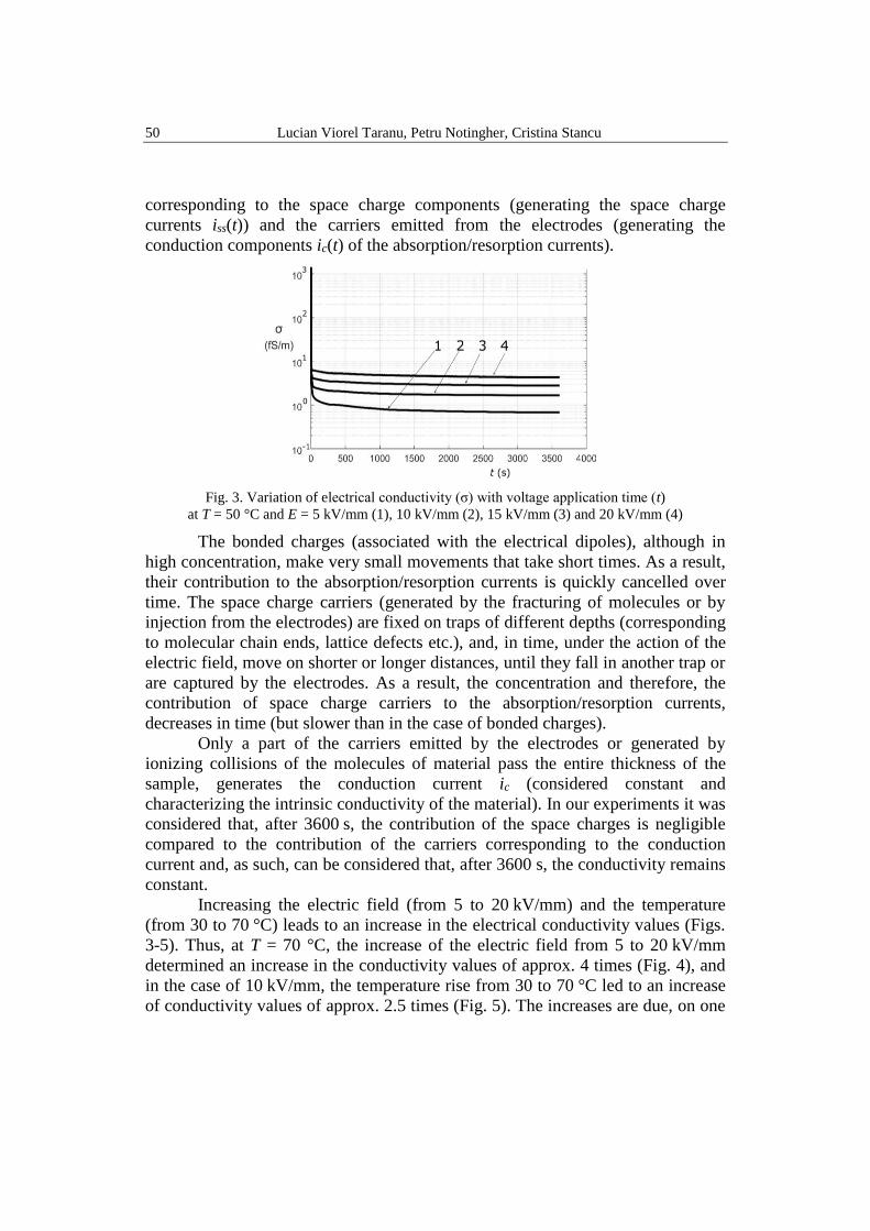
To obtain values closer to the experimental ones, a new empirical equation

for the electrical conductivity σ(E,T) is proposed:

( )( )( )

E

EbaT

kT

EATE a ln sinh

exp,+

−= (10)

The new values of A, Ea, a and b are presented in Table 2 (equation (10)),

and the variation curves of the conductivity with E and T in Fig. 6.

Table 1

Values of electrical conductivity σ of XLPE samples for different

temperatures (T) and electric fields (E)

No. T (oC) E (kV/mm) σ (fS/m)

1 30 5 0.513

2 30 20 3.910

3 50 5 0.687

4 50 20 4.460

5 50 10 1.680

6 70 5 1.420

7 70 20 5.920

8 70 10 2.830

Table 2

Values of A, Ea, a, b and α related to equations (6) – (10)

Eq. T (°C) A (S/m) Ea (eV) a (1/K) b (-) α (-)

(6) ≤ 50

0.5 0.5347 –2.8746∙10-9 1.147∙10-6

- ≥ 50 –2.8535∙10-9 1.1688∙10-6

(7) ≤ 50

0.1259 0.5336 –1.2673∙10-5 0.0054 - ≥ 50

(8) ≤ 50

0.0132 0.5374 –2.1043∙10-4 0.0978 - ≥ 50

(9) ≤ 50 25

0.55 –1.543∙10-16 5.1195∙10-14 0.045

≥ 50 22.5 –1.3696∙10-17 4.9247∙10-15 0.111

(10) ≤ 50

9.5234∙10-16 0.55 –0.0034 3.406 -

≥ 50 –0.0023675 3.0685 -

It can be seen that the values of the electrical conductivity calculated with (10)

(curve 6, Fig. 6) are very close to the ones experimentally determined (curve 1,

Fig. 6).

The relative differences between the calculated σc(E,T) and experimental

σm(E,T) values of the conductivity, determined with the equation:


( ) ( )

( ) %100

,

,,

−=

TE

TETE

m

mc

rel (11)

have average values below 10 %, for all the temperatures. The maximum value of

the relative difference (26.7 %) was obtained for E = 5 kV/mm and T = 70 oC, and

the minimum one (0.2 %) – for E = 15 and 20 kV/mm and T = 70 oC.

Consequently, it can be said that for values of the electric field between 5 and

20 kV/mm, the calculated values of the conductivity using equation (10) are

closest to the experimental ones.

The quantities A, Ea, a and b, involved in equation (10) were determined

using the conductivity values experimentally determined for fields between 5 and

20 kV/mm. As, in the case of cables and joints insulation, values of E can be

lower than 5 kV/mm or higher than 20 kV/mm, the conductivity values were

calculated also, for fields between 1 and 5 kV/mm and 20 and 40 kV/mm. The

experimental conductivity values were obtained by prolonging the experimental

curves (Fig. 7) using interpolating functions associated with the experimental data

points (determined with the MATLAB software).

For electric field values lower than 5 kV/mm, the differences between the

calculated and experimental values are higher than those corresponding to fields

between 5 and 20 kV/mm. Instead, for E > 20 kV/mm these differences are lower,

reaching up to 0.5 % for E = 40 kV/mm and T = 30 oC (Fig. 7, curves 1 and 2).

Consequently, equation (10) can be used for any field lower than 40 kV/mm.

Certainly, for a more accurate verification, new tests should be done, at fields

lower than 5 kV/mm and higher than 20 kV/mm.

Fig. 7. Variation of electrical conductivity σ with electric field E experimental (curves 1, 3

and 5) and calculated ones (curves 2, 4 and 6) with equation (10) at T = 30 °C (curves 1, 2),

50 °C (curves 3, 4) and 70 °C (curves 5, 6)


5. Conclusions

Experiments performed on cross-linked polyethylene samples show that

the electrical conductivity values are strongly influenced by those of the electric

field and temperature.

In the case of tested XLPE samples, empirical equations proposed in

literature for electric conductivity of polymers lead - for fields between 5 and

20 kV/mm and temperatures between 30 and 70 oC - to important errors (even

above 60 %).

The new empirical equation proposed in the paper allows the electrical

conductivity values calculation with higher accuracy and for larger intervals of E,

the average differences between the calculated and experimental values being

under 10 %.

Acknowledgements

The authors express their acknowledgement to ICME ECAB Bucharest for

technical support regarding the samples manufacturing and to the Laboratory of

Innovation Technology (LIT) of the University of Bologna for the conductivity

measurement setup and assistance.

R E F E R E N C E S

[1]. R. Bartnikas, K.D.Srivastava, Power and Communication Cables. Theory and Applications,

IEEE Press, New York, 2000.

[2]. P.V.Notingher, Materiale pentru Electrotehnica (Materials for Electrotechnics), Vol. 2,

Politehnica Press, 2005.

[3]. L.Dechamps, R. Michel, L. Lapers, Development in France of High Voltage Cables with

Synthetic insulation, CIGRE, Paris, 1980, report 21-06.

[4]. U. Amerpoh, H. Koberh, C.van Hove, H. Schadlich, G. Ziemeck, Development of Polyethylene

Insulated Cables for 220 kV and higher Voltages, CIGRE, Paris, 1980, Report 21-11.l.

[5]. C. Stancu, P.V. Notingher, P. Notingher, M. Lungulescu, Space Charge and Electric Field in

Thermally Aged Multilayer Joints Model, IEEE Transactions on Dielectrics and Electrical

Insulation,Vol. 23, No. 2, 2016, pp.633-644.

[6]. M.G. Plopeanu, P.V. Notingher, C. Stancu, S. Grigorescu, Underground power cable

insulation electrical lifetime estimation methods, Scientific Bulletin of University

POLITEHNICA of Bucharest, Series C: Electrical Engineering and Computer Science, Vol.

75, Iss. 1, 2013, pp. 233-238, ISSN 1454-234x (B+).

[7]. C. Rusu-Zagar, P.V. Notingher, S. Busoi, M. Lungulescu, G. Rusu-Zagar, Rapid Estimation of

Lifetime and Residual Lifetime for Silicone Rubber Cable Insulation, UPB Scientific

Bulletin, Series C, Vol. 79, Iss. 1, 2017, pp.181-196, ISSN 2286-3540.

[8]. L.A. Dissado, J.e. Fothergill, Electrical Degradation and Breakdown in Polymers, lEE P.

Peregrinus, London, 1992.

[9]. B. Hilczer, J. Malecki, Electrets, Elsevier, Warsaw, 1986.

[10]. G. Blaise, “Charge localization and transport in disordered dielectric materials”, J.

Electrostatics, vol. 50, 2001, pp. 69-89.


[11]. M.C. Lanca, Electrical Ageing Studies of Polymeric Insulation for Power Cables, PhD

Thesis, Universida de Nova de Lisboa, Lisbon, 2002.

[12]. G.C. Montanari, G. Mazzanti, F. Palmieri, A. Motori, G. Perego, S. Serra, Space-charge

trapping and conduction in LDPE, HDPE and XLPE, J. Phys. D: Appl. Phys., vol. 34, 2001,

pp. 2902-2911.

[13]. C. Stancu, P. V. Notingher, Influence of the Surface Defects on the Absorption/Resorption

Currents in Polyethylene Insulations, Scientific Bulletin of University POLITEHNICA of

Bucharest, Series C: Electrical Engineering and Computer Science, vol. 72, Iss. 2, 2010, pp.

161 – 170.

[14]. C. Stancu, Méthodes d’estimation de l’état de vieillissement des câbles d’énergie, Editions

universitaires europeennes, LAMBERT Academic Publishing, Riga, 2018. [15]. C. Stancu, P.V.Notingher, P. Notingher jr., Computation of the Electric Field in Aged

Underground Medium Voltage Cable Insulation, IEEE Transactions on Dielectrics and

Electrical Insulation, Vol. 20, Issue 5, 2013, pp. 1530-1539.

[16]. C. Stancu, P.V.Notingher, P.P. Notingher, M.Lungulescu, Space Charge and Electric Field in

Thermally Aged Multilayer Joints Model, IEEE Transactions on Dielectrics and Electrical

Engineering, Vol. 23, No. 2, 2016, pp. 633-644.

[17]. S. Boggs, D. H. Damon, J. Hjerrild, J. T. Holboll, and M. Henriksen, “Effect of insulation

properties on the field grading of solid dielectric DC cable”, IEEE Trans. Power Deliv., vol.

16, no. 4, 2001, pp. 456–461.

[18]. C. Stancu, P. V. Notingher, L. M. Dumitran, L. Taranu, A. Constantin, and A. Cernat,

“Electric field distribution in dual dielectric DC cable joints”, in 2016 IEEE International

Conference on Dielectrics (ICD), 2016, pp. 402–405.

[19]. N. Adi, G. Teyssedre, T. T. N. Vu, and N. I. Sinisuka, “DC field distribution in XLPE-

insulated DC model cable with polarity inversion and thermal gradient”, in 2016 IEEE

International Conference on High Voltage Engineering and Application (ICHVE), 2016, pp.

1–4.

[20]. Z. Xu, W. Choo, and G. Chen, “DC electric field distribution in planar dielectric in the

presence of space charge”, in 2007 IEEE International Conference on Solid Dielectrics,

2007, pp. 514–517.

[21]. O. L. Hestad, F. Mauseth, and R. H. Kyte, “Electrical conductivity of medium voltage XLPE

insulated cables”, in 2012 IEEE International Symposium on Electrical Insulation, 2012, pp.

376–380.

[22]. G. Jiang, J. Kuang, and S. Boggs, “Evaluation of high field conduction models of polymeric

dielectrics”, in 2000 Annual Report Conference on Electrical Insulation and Dielectric

Phenomena (Cat. No.00CH37132), vol. 1, pp. 187–190.

[23]. T. N. Vu, G. Teyssedre, B. Vissouvanadin, S. Roy, and C. Laurent, “Correlating conductivity

and space charge measurements in multi-dielectrics under various electrical and thermal

stresses”, IEEE Trans. Dielectr. Electr. Insul., vol. 22, no. 1, 2015, pp. 117–127.

[24]. T. T. N. Vu, G. Teyssedre, S. Le Roy, and C. Laurent, “Maxwell–Wagner Effect in Multi-

Layered Dielectrics: Interfacial Charge Measurement and Modelling”, Technologies, vol. 5,

no. 4, 2017, pp. 27-42.

Documents

THE INFLUENCE OF ELECTRIC FIELD AND TEMPERATURE ON …