Embed Size (px)
Citation preview

The Journal of Systems and Software 132 (2017) 226–252
Contents lists available at ScienceDirect
The Journal of Systems and Software
journal homepage: www.elsevier.com/locate/jss
Cross-validation based K nearest neighbor imputation for software
quality datasets: An empirical study
Jianglin Huang
a , ∗, Jacky Wai Keung
a , Federica Sarro
b , Yan-Fu Li c , Y.T. Yu
a , W.K. Chan
a , Hongyi Sun
d
a Department of Computer Science , City University of Hong Kong , Hong Kong , China b Department of Computer Science , University College London , London , UK c Department of Industrial Engineering , Tsinghua University , Beijing , China d Department of Systems Engineering and Engineering Management , City University of Hong Kong, Hong Kong , China
a r t i c l e i n f o
Article history:
Received 16 February 2016
Revised 6 July 2017
Accepted 12 July 2017
Available online 13 July 2017
Keywords:
Empirical software engineering estimation
KNN
Imputation
Cross-validation
Missing data
a b s t r a c t
Being able to predict software quality is essential, but also it pose significant challenges in software engi-
neering. Historical software project datasets are often being utilized together with various machine learn-
ing algorithms for fault-proneness classification. Unfortunately, the missing values in datasets have nega-
tive impacts on the estimation accuracy and therefore, could lead to inconsistent results. As a method
handling missing data, K nearest neighbor ( K NN) imputation gradually gains acceptance in empirical
studies by its exemplary performance and simplicity. To date, researchers still call for optimized param-
eter setting for K NN imputation to further improve its performance. In the work, we develop a novel
incomplete-instance based K NN imputation technique, which utilizes a cross-validation scheme to opti-
mize the parameters for each missing value. An experimental assessment is conducted on eight qual-
ity datasets under various missingness scenarios. The study also compared the proposed imputation ap-
proach with mean imputation and other three K NN imputation approaches. The results show that our
proposed approach is superior to others in general. The relatively optimal fixed parameter settings for
K NN imputation for software quality data is also determined. It is observed that the classification accu-
racy is improved or at least maintained by using our approach for missing data imputation.
© 2017 Elsevier Inc. All rights reserved.
Abbreviations: BMI, Bayes Multiple Imputation; CA, Classification Accuracy;
CC k NNI, Complete-case based K NN Imputation; CK, Chidamber and Kemerer object-
oriented metric; CVB k NNI, Cross-validation based K NN Imputation; D k NNI, Default
K NN Imputation; FP, Fault-proneness; FWG k NNI, Feature Weighted Grey based K NN
Imputation; G3D, GRA-based distance, K = 3 with Dudani adaptation based impu-
tation; GRA, Grey Relational Analysis; GRC, Grey Relational Coefficient; GRG, Grey
Relational Grade; IC k NNI, Incomplete-case based K NN Imputation; IDWM, Inverse
Distance Weighted Mean; IRWM, Inverse Rank Weighted Mean; K NN, K Nearest
Neighbor; LOC, Lines of Code; MAR, Missing At Random; MCAR, Missing Completely
At Random; MDT, Missing Data Treatment; MEI, Mean Imputation; MI, Mutual In-
formation; MM, Missingness Mechanism; MP, Missingness Pattern; MR, Missing-
ness Ratio; NI, Non-ignorable; PROMISE, PRedictOr Models In Software Engineering;
RMSE, Root Mean Square Error; RQ, Research Question; SEE, Software Engineering
Estimation; SVM, Support Vector Machine. ∗ Corresponding author.
E-mail addresses: [email protected] , [email protected]
(J. Huang), [email protected] (J.W. Keung), [email protected]
(F. Sarro), [email protected] (Y.-F. Li), [email protected] (Y.T. Yu),
[email protected] (W.K. Chan), [email protected] (H. Sun).
1
s
i
f
t
c
m
l
i
(
i
a
d
i
m
d
n
http://dx.doi.org/10.1016/j.jss.2017.07.012
0164-1212/© 2017 Elsevier Inc. All rights reserved.
. Introduction
In the domain of empirical software engineering and its related
oftware quality estimation, researchers have devoted to predicting
mportant quality-related variables, such as the fault count or if the
ault-proneness exists, etc. Most empirical software engineering es-
imation builds statistical or machine learning models on histori-
al data ( Sentas and Angelis, 2006 ). Meanwhile, the software com-
unity has accumulated a myriad of software project quality re-
ated data for academic research, such as the PROMISE data repos-
tories. Unfortunately, due to scarcity of software engineering data
Myrtveit et al., 2001 ), the significant occurrence of missing values
n software datasets or known as “missingness” gradually becomes
n unavoidable issue ( Khoshgoftaar and Van Hulse, 2008 ). In ad-
ition, many properties in software engineering datasets are often
ndirectly measured, which leads to more frequent and complex
issingness pattern to occur ( Mockus, 2008 ).
Many estimation models cannot directly handle the missing
ata values; therefore, it leaves the data-preprocessing step very
ecessary for modern estimation process in software engineer-

J. Huang et al. / The Journal of Systems and Software 132 (2017) 226–252 227
i
t
i
n
(
o
2
d
e
C
a
p
f
i
a
(
i
K
t
a
p
d
a
b
T
n
r
r
i
T
t
m
a
s
t
w
i
p
f
f
i
s
t
s
t
a
n
n
S
r
c
p
r
s
l
r
(
b
M
t
a
t
t
o
d
c
m
i
a
t
w
a
a
n
T
t
k
i
2
p
t
s
m
e
h
S
l
2
m
f
p
t
a
i
d
o
a
v
i
b
i
d
p
ng. For example, a well-known technique called listwise dele-
ion, had been widely adopted for handling missing values dur-
ng data-preprocessing, but it potentially impairs the complete-
ess of data and introduces undesirable biases in estimation
Huang et al., 2015 ). By contrast, missing data imputation meth-
ds replace missing variables by artificial estimates ( Song et al.,
008 ); at the same time maintain the data completeness. Nowa-
ays, more complex imputation approaches, such as random for-
st ( Stekhoven and Bühlmann, 2012 ), neural network ( Rey-del-
astillo and Cardeñosa, 2012 ), decision trees ( Deb and Liew, 2016 ),
nd low-rank matrix factorization ( Jing et al., 2016 ), have been pro-
osed to handle the missingness issue in the applications of bioin-
ormatics, education, ecology, energy, traffic and software engineer-
ng, etc.
When compared to mean imputation (MEI), novel approaches
re still lacking popularity in software engineering estimation (SEE)
Khatibi Bardsiri et al., 2013; Kocaguneli et al., 2013a ), one of which
s the K nearest neighbor ( K NN) imputation. The main advantage of
NN imputation is that it is simple and free of parametric assump-
ions required otherwise. It could adapt to distinct types of vari-
bles or features known to be important in estimation. K NN im-
utation had been specially applied in real-world application as a
ata-preprocessing step in governmental or national surveys, such
s reported in Chen and Shao (20 0 0) . Its performance has also
een widely analyzed in the domain of SEE ( Strike et al., 2001;
wala et al., 2005 ). Since most of the empirical software engi-
eering datasets are relatively small or medium-sized, the newer
obust approaches, like random forest, neural network, and low-
ank matrix factorization as less than relevant. The cost of apply-
ng these sophistical approaches in practice is also unpredictable.
he majority of the previous SEE studies only applied K NN imputa-
ion with fixed parameters when dealing with incomplete software
easurement data.
Song and Shepperd (2007) once evaluated a K NN imputation
pproach with several key features classification in small-sized
oftware effort datasets. More recently, Van Hulse and Khoshgof-
aar (2014) extended the flexibility of K NN imputation for the soft-
are quality datasets, using incomplete-instance for missing data
mputation instead of complete-instance to provide a relatively su-
erior performance. Unfortunately, the parameter setting of the
ormer K NN imputation approaches was generally predetermined
or each imputation, regardless of its features or the types of miss-
ngness being imputed. While in the specialized K NN imputation
tudies, numerous efforts have been made to improve the impu-
ation performance. The major improvement drives from two re-
earch directions ( Zhang, 2012 ):
- Searching for the most similar K nearest neighbors for a given
missing value;
- Final adaptation from the selected neighbors.
Both two directions are about the parameter setting in K NN es-
imator, including the distance measure, the choice of K , and the
daptation method. The 1st direction is the K NN algorithm ker-
el. Literature review shows that the current rule of searching the
eighbors in SEE is mostly based on Minkowski distance measure.
ome specialized studies of K NN imputation show that the grey
elational analysis (GRA) based distance, is more appropriate to
apture the ‘nearness’ ( Huang and Lee, 20 04 ). Caruana (20 01) has
ointed out that the K NN imputation could not always be supe-
ior with any possible distance measures. The choice of the K is
ubject to controversy recently. The related studies often prepopu-
ate that the K from limited experience and empirical studies, other
esearchers argues the potential choices of K to be √
N , N > 100
Lall and Sharma, 1996 ), where N is the sample size of the dataset
eing investigated.
The 2nd direction is computation using the selected neighbors.
issing data imputation using median/mean is a naive and effec-
ive adaptation in some cases. Using rank or distance as weight is
lso popular in literature ( Kocaguneli et al., 2012b ). Unfortunately,
here is no such a guarantee that one of these adaptations results
he best option. Therefore, researchers turned to build ensembles
f multi-adaptation methods to empirically find the best one un-
er certain circumstance ( Kocaguneli et al., 2012b; 2013b ).
In this study, we focus and present a novel approach named as
ross-validation based K NN imputation (CVB k NNI) to conquer the
ajor drawback of existing K NN imputation approaches: an inabil-
ty of adapting the parameter setting to the data. CVB k NNI utilizes
cross-validation scheme to search for the optimal parameter set-
ing for estimating each missing value. CVB k NNI is also compared
ith three other K NN imputation approaches in the presence of
rtificial missingness scenarios. This empirical study:
- Introduce CVB k NNI, a novel approach with an adaptive param-
eter setting, applicable to software quality prediction and mod-
eling. The internal design of CVB k NNI includes both imputation
ordering and various parameters of K NN imputation estimator.
Based on the estimators returned from the CVB k NN algorithm,
a fixed parameter setting is discovered to be recommendable
for K NN imputation in software quality datasets.
- Validate that the missingness scenario could be a critical fac-
tor that significantly impacts the imputation performance un-
der certain circumstance. A thorough statistical analysis is pre-
sented to compare with the different K NN imputation ap-
proaches under different missingness scenarios.
In the remaining parts of the work, background and review
re presented in Section 2 . Section 3 introduces the CVB k NNI, the
ovel missing data imputation technique proposed in this study.
he experimental design is described in Section 4 . Section 5 fur-
her presents the experimental results. Section 6 discusses the
nown threats to validity in this empirical study. At last, the work
s concluded with future work in Section 7 .
. Background
In this section, we define the terminology and provide a sim-
le review. This section covers three aspects: an introduction to
he missingness mechanisms and patterns, the review of recent
pecialized K nearest neighbor ( K NN) imputation studies and the
issing data treatments (MDTs) research in software engineering
stimation (SEE).
The missingness mechanisms (MM) and patterns (MP) explain
ow the missingness is summarized and classified in literature.
electing the proper approach to deal with missing values is re-
ated to the assumption of the mechanism and pattern ( Song et al.,
005 ). The introduction of MM, MP and ratio helps build different
issingness scenarios. The performance of different MDTs could be
urther validated under these scenarios then. In the section of ex-
eriment design, the incomplete datasets are synthetized according
o the various missingness scenarios.
The K NN imputation, free of data distribution assumption, is
n important single hot-deck imputation technique. Popular single
mputation approaches also contain mean imputation (MEI), me-
ian imputation and the ones based on stochastic regression meth-
ds, etc. Single imputation cannot tolerate the variability of char-
cterization of the imputed values. Concisely, it is unable to pro-
ide valid confidence intervals of the imputed values. Therefore,
ts simultaneous accuracy as well as robustness become a concern
ut difficult to address adequately. As an alternative of single data
mputation, multiple imputation generates many different imputed
atasets and then computes the final estimation result of the com-
lete dataset by applying appropriate adaptation strategy, which

228 J. Huang et al. / The Journal of Systems and Software 132 (2017) 226–252
u
o
r
c
e
h
d
m
W
t
T
i
w
p
m
M
m
2
o
i
e
N
u
(
A
t
c
a
c
d
t
i
d
t
K
Z
t
f
n
i
b
a
m
p
K
e
t
F
c
d
p
a
e
l
i
t
f
M
i
t
is considered more complex in its application. Novel techniques,
for example, iterative imputation, gain increasing popularity in re-
cent years, and they improve the estimation accuracy by iteratively
searching for the optimal estimates until convergence.
As the specialized K NN imputation research has been evolved
in years, yet it has been applied in contemporary SEE studies.
Huang et al. (2015) has found that MEI monopolizes the imputa-
tion approaches in recent software effort estimation studies. A re-
view of the other MDTs in SEE studies is presented at last.
2.1. Missingness mechanisms and patterns
Missingness mechanisms (MMs) and patterns (MP) make as-
sumptions about the distribution and types of missing values
( Song et al., 2008 ). The judgment of MM helps assess what im-
putation approach may be adopted ( Song et al., 2005 ). The MM
concerns if the missingness is related to the key variable or not.
It is critical as it determines how difficult handling missing val-
ues is ( Song and Shepperd, 2007 ). There are three mechanisms
( Little and Rubin, 2002 ): missing completely at random (MCAR),
missing at random (MAR) and non-ignorable (NI). To present the
MM with formal notations, assume the real-valued software data
we intend to collect as X = { x i } , 1 ≤ i ≤ N, and X has observed and
missing parts. Consider the missing parts in X have the values
that are unobserved, we use the missing data indicator M = { m i } ,where m i = { 0 if x i isunobserved
1 if x i is observed
, to denote the observation out-
come. The missingness mechanism is characterized by the condi-
tional probability distribution of M given X , i.e. p ( M | X, ψ), where
ψ refers to the unknown parameters.
MCAR means there is no difference between the distribution of
observed and missing values ( Song et al., 2008 ). In other words,
missingness does not depend on either observed values or missing
values of X , thus p( M| X, ψ ) = p( M, ψ ) .
MAR means that missingness only depends on the observed
values of other variable(s), not the missing ones. It does not fulfil
the condition of MCAR (it must depend on at least one variable).
Assuming that m is a potential value (vector) for M , then ∀ m ∈ {1,
0} N and ∀ x, y ∈ R
N with H( x, y ) = m : p( M = m | x ) = p( M = m | y ) ,where H ( x, y ) denotes the Hamming difference vector of variables
x and y , that has 0 in the positions where x and y differ and 1 in
the positions where they coincide.
NI represents the situation that neither MCAR nor MAR holds
( Valdiviezo and Van Aelst, 2015 ). Missingness only depends on the
unobserved values, i.e. their real values. Even accounting for all the
available observed information, the reason for observations being
missing still depends on the unseen missingness.
Generally, there are two types of multivariate missingness pat-
terns (MPs): monotone and general (non-monotone) ( Song and
Shepperd, 2007; Van Buuren, 2012 ). An MP is said to be mono-
tone if an instance x i , could be ordered such that if x i, p is missing
then all values in x i with p ′ > p are missing simultaneously. It could
occur in longitudinal studies. In software quality datasets, if a ma-
jor basic measure is missing, all the following derived ones will
not exist. In the general pattern, missing data can occur anywhere
and no special structure appears regardless of how the variables
are arranged. The type of MP may affect the selection of MDTs.
Strike et al. (2001) found the MDTs tend to perform worse with
monotone pattern. This issue will be discussed in the experiment
analysis.
Some imputation approaches cannot handle specific MMs or
MPs appropriately ( Song and Shepperd, 2007 ). MCAR could be
tested by Little and Rubin (2002) ’s multivariate test under certain
strict conditions. Unfortunately, it is hardly applicable to validate
the exact MM and MP before adopting an MDT ( Song et al., 2005 ).
Identifying MM is difficult since the prior distribution is in general
nknown. Hardly it is possible to guarantee that none of MCAR, NI
r MAR could exist in software quality data. Generally, the MM in
eal datasets is often to be either NI or MAR, while the MP often
onsists both general and monotone, but not always tenable ( Song
t al., 20 05; 20 08; Strike et al., 20 01 ). Song et al. (20 08) illustrated
ow NI and MAR may happen in software practice. Suppose un-
er the politic pressure, software engineers prefer not to report
any high fault rates and then intend to make the values missing.
hile some software metrics are too difficult and time-consuming
o collect, which, therefore, may cause the values missing as well.
hey explain how NI could happen when missingness depends on
ts real values. MAR could occur if only the small-sized projects
ere less likely to report fault rates than the large well-organized
rojects. It exemplifies MAR that missingness depends on the non-
issing project feature: size. Therefore, this study simulates the
Ps (monotone and general) and MMs (MCAR, MAR, and NI) si-
ultaneously to conduct the experiments.
.2. K NN imputation improvement
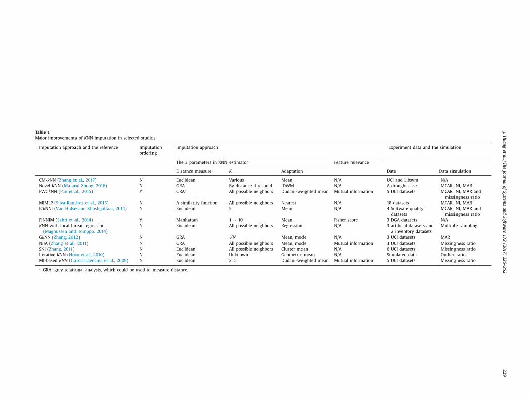
In this section, 12 former studies about specific improvements
n K NN imputation are chronologically selected and summarized
n Table 1 in terms of the imputation estimator design and the
xperimental data simulation (missingness injection) approaches.
ote that this is not an exhaustive search on recent studies. We
se the keywords combination:
knn OR k-nn OR knni OR “nearest neighbo
∗”) AND (imput ∗)ND (missing)
o search the related recent papers. Only the qualified works that
oncentrates on k NN imputation improvement for numeric vari-
bles are kept. The studies in Table 1 are simply summarized ac-
ording to the K NN imputation technique design and experiment
esign. In specific, García-Laencina et al. (2009) proposed a fea-
ure weighted distance measure based on mutual information (MI)
n K NN imputation. Their experiment validated that both missing
ata imputation and classification task were improved by their
echnique. Hron et al. (2010) adopted the Aitchison distance in
NN imputation and found that it is not robust against outliers.
hang et al. (2011) proposed a nonparametric iterative imputa-
ion algorithm (NIIA) to impute missing value and found it outper-
orms the other methods in general. Zhang (2011) proposed shell
eighbors imputation (SNI) which fills in an incomplete instance
n a given dataset by only using its left and right nearest neigh-
ors with respect to each other. SNI was found to be better than
traditional K NN imputation. Zhang (2012) changed the distance
easure to grey distance and found its advantage in capturing the
roximity relationship. Magnussen and Tomppo (2014) calibrated
NN imputation with local linear regression in the context of for-
st science. The new technique presented improved correlation be-
ween imputation and its real value. Sahri et al. (2014) proposed
INNIM in the context of dissolved gas analysis, in which they
learly addressed two important components of imputation: or-
ering and estimator. Silva-Ramírez et al., (2015) combined multi-
layer perceptron and K NN algorithms in missing data imputation
nd conducted their experiment on simulated datasets with differ-
nt missingness patterns. Ma and Zhong (2016) proposed a corre-
ated degree model to extract K nearest neighbors for imputation
n the context of natural disaster science. Zhang et al., (2017) fur-
her incorporated correlation matrix in K NN imputation design and
ound its efficiency compared with the traditional K NN imputation.
Regarding to imputation ordering, one important component in
DT, 10 out of the 12 studies did not consider using it in K NN
mputation. As for the K NN parameter: distance measure, besides
he classic Euclidean distance and Manhattan distance measures,
J. H
ua
ng et
al. / T
he Jo
urn
al o
f Sy
stems a
nd So
ftwa
re 13
2 (2
017
) 2
26
–2
52
22
9
Table 1
Major improvements of K NN imputation in selected studies.
Imputation approach and the reference Imputation
ordering
Imputation approach Experiment data and the simulation
The 3 parameters in K NN estimator Feature relevance
Distance measure K Adaptation Data Data simulation
CM- k NN ( Zhang et al., 2017 ) N Euclidean Various Mean N/A UCI and Libsvm N/A
Novel K NN ( Ma and Zhong, 2016 ) N GRA By distance threshold IDWM N/A A drought case MCAR, NI, MAR
FWG k NN ( Pan et al., 2015 ) Y GRA ∗ All possible neighbors Dudani-weighted mean Mutual information 5 UCI datasets MCAR, NI, MAR and
missingness ratio
MIMLP ( Silva-Ramírez et al., 2015 ) N A similarity function All possible neighbors Nearest N/A 18 datasets MCAR, NI, MAR
IC k NNI ( Van Hulse and Khoshgoftaar, 2014 ) N Euclidean 5 Mean N/A 4 Software quality
datasets
MCAR, NI, MAR and
missingness ratio
FINNIM ( Sahri et al., 2014 ) Y Manhattan 1 ∼ 10 Mean Fisher score 3 DGA datasets N/A
K NN with local linear regression
( Magnussen and Tomppo, 2014 )
N Euclidean All possible neighbors Regression N/A 3 artificial datasets and
2 inventory datasets
Multiple sampling
G k NN ( Zhang, 2012 ) N GRA √
N Mean, mode N/A 3 UCI datasets MAR
NIIA ( Zhang et al., 2011 ) N GRA All possible neighbors Mean, mode Mutual information 3 UCI datasets Missingness ratio
SNI ( Zhang, 2011 ) N Euclidean All possible neighbors Cluster mean N/A 6 UCI datasets Missingness ratio
Iterative K NN ( Hron et al., 2010 ) N Euclidean Unknown Geometric mean N/A Simulated data Outlier ratio
MI-based KNN ( García-Laencina et al., 2009 ) N Euclidean 2, 5 Dudani-weighted mean Mutual information 5 UCI datasets Missingness ratio
∗ GRA: grey relational analysis, which could be used to measure distance.

230 J. Huang et al. / The Journal of Systems and Software 132 (2017) 226–252
2
e
t
p
2
i
t
t
o
c
Y
e
K
F
s
q
f
i
a
t
p
n
S
(
i
c
m
n
a
t
T
r
p
v
M
a
w
d
e
p
d
o
i
(
i
t
p
w
i
t
(
c
n
t
d
a
i
i
o
4 out of 12 studies preferred the grey relational analysis (GRA)
based similarity measure to capture the ‘nearness’ of neighbors. In
terms of the choice of K , half of the studies predefined the value
of K and the other half preferred to use overall available neigh-
bors for adaptation. As for the adaptation methods, instead of us-
ing the mean, various methods are adopted, such as regression-
based, cluster-based and Dudani weighted mean, etc. Meanwhile,
less than half of the studies considered the issue of feature rele-
vance in searching of the nearest neighbors.
As for the experiment design, the experiment data and data
simulation methods are quite consistent among the studies. The
UCI data, a famous machine learning data repository, has been
experimented on by half of them. The rest datasets belong to
diverse professional domains, such as biology, energy, and soft-
ware. Only Song and Shepperd (2007) and Van Hulse and Khosh-
goftaar (2014) evaluate their new proposed K NN imputation ap-
proaches in the domain of empirical SEE. The missingness in-
jection criteria for data simulation majorly consider the missing-
ness mechanism (MM) and ratio (MR), and only Song and Shep-
perd (2007) ’s research took into account of the missingness pat-
tern (MP). However, only Pan et al. (2015) and Song and Shep-
perd (2007) empirically analyzed the impact of missingness injec-
tion on imputation performance.
To sum, for current K NN based missing data imputation re-
search, it is common to see the overall methodology design is frag-
mented. Researchers turn to prefer different experiment evaluation
criteria in studies, which, therefore, causes the corresponding tech-
nical contribution hardly justified. As for the improvement on K NN
imputation, none of the studies systematically analyze the impacts
imputation ordering in K NN imputation performance. There is still
no common solution to select the optimized K NN parameters for
imputation. Although researchers prefer to use various missingness
scenarios to test their techniques, the significance of the impacts of
the missingness scenarios are often neglected.
Two of the recent imputation approaches in Table 1 , FWG k NN
imputation (FWG k NNI) and IC k NNI, which could be repeated
according to corresponding experiment design, are utilized in
our experimental design as competitors to CVB k NNI. Pan et al.
(2015) proposed a feature weighted grey based K NN iterative im-
putation (FWG k NNI) approach, in which they combined feature
relevance and grey relational analysis (GRA) based distance mea-
sure in the estimator. MEI is used to have a preliminary estimate
of the missing values. The nearest neighbors are extracted from
the dataset which contains all the available instances, except the
one that is to be imputed. The data is updated after each im-
putation iteration, and the iteration repeats until all the missing
values are imputed. The capacity of FWG k NNI is improved com-
pared with the 4 other competitors used in their study, includ-
ing F k MI ( Li et al., 2004 ), I k NNI ( Brás and Menezes, 2007 ), GBNN
( Huang and Lee, 2004 ) and G k NN ( Zhang, 2012 ). Missing data in-
jection with various MMs is also considered in their data simula-
tion.
Van Hulse and Khoshgoftaar (2014) proposed an incomplete-
case (instance) based K NN imputation (IC k NNI) in the context of
software quality data, and raised the issue of missing data in em-
pirical SEE research once again. Instead of using all available com-
plete instances, IC k NNI searches the nearest neighbor of each in-
stance from the incomplete data. Their results showed that the
complete-case based K NN imputation (CC k NNI) is far less superior
than the imputation approach based on both incomplete and com-
plete instances, i.e . the IC k NNI. The parameters of IC k NNI is pre-
dominated as well: Euclidean distance, K = 5, with mean adapta-
tion. This paper did not consider comparing the IC k NNI with more
imputation approaches, even the MEI.
c
.3. Studies of missing data treatment in software engineering
stimation context
Missing data treatment (MDT) has been mostly discussed in
he data-driven studies of social science, biology, psychology, trans-
ortation, and behavioral science ( Poloczek et al., 2014; Sahri et al.,
014; Suyundikov et al., 2015 ). MDT is considered as an evolv-
ng area in software engineering estimation (SEE) research for less
han 15 years. Less attention has been focused on MDT methods
hemselves. In a more recent study, Huang et al. (2015) found that
nly some of the former software effort estimation studies have
onsidered the significance of the MDTs, of which only Minku and
ao (2011) used K NN imputation in data-reprocessing during the
stimation modeling. By contrast, Troyanskaya et al. (2001) applied
NN imputation in the estimation of missing DNA microarrays, and
inley et al. (2006) even explored its utility in the domain of forest
cience.
Empirical analysis about missingness characteristics in software
uality data are even rare. Song et al. (2008) emphasized that
or large-sized samples with MCAR mechanism, listwise deletion
s considered appropriate, but the assumption of MCAR is ideal
nd less applicable in real software datasets. Additionally, if ei-
her NI or MAR exists, which is more probable, missing data im-
utation is relatively a better option then. However, imputation
eeds more thorough computational analysis ( Myrtveit et al., 2001;
trike et al., 2001 ), and the prediction error may be introduced
Mittas and Angelis, 2010 ). MEI is efficient and has been involved
n SEE as the most popular imputation approach; however, it will
ause bias to data. MEI simply replaces the missing values with the
ean of other values in the same feature.
K NN imputation is then used as an advanced imputation tech-
ique in SEE ( Minku and Yao, 2011 ). Strike et al. (2001) compared
nd tested various parameter settings in K NN imputation. The set-
ings took account of Euclidean and Manhattan distance measures.
he MM is simulated from 206 real-world software datasets. The
esults indicated that listwise deletion is reasonable but may not
rovide the best performance. They called for validating more ad-
anced imputation techniques on software engineering datasets.
yrtveit et al. (2001) evaluated the closest neighbor imputation on
real-world incomplete dataset and showed that compared to list-
ise deletion, K NN imputation is the right option only when the
ataset has too much missingness. Cartwright et al. (2003) then
xamined MEI and K NN imputation for two real industrial incom-
lete datasets and found that K NN imputation provides better pre-
iction than MEI does. Twala et al. (2005) , on the other hand, rec-
mmended adopting MEI when massive missingness exists and us-
ng K NN imputation when sparse missingness exists. Song et al.
2005) argued that the impact of MM on imputation performance
s not always that obvious. Jönsson and Wohlin (2006) examined
hat K NN imputation performs better in high dimensional incom-
lete datasets.
Li et al. (2007) found that more missingness in data could
orsen the accuracy of K NN imputation. They appealed to future
nvestigation of the impact of missingness scenarios with more dis-
ance and adaptation in K NN imputation. Continuously, Song et al.
2008) further confirmed that K NN imputation provides high ac-
uracy. Khoshgoftaar and Van Hulse (2008) analyzed the effective-
ess of various imputation approaches, including MEI, K NN impu-
ation and Bayes multiple imputation (BMI), on two real software
atasets. Their results indicate BMI is better than K NN imputation
nd MEI. Overall, most researchers did not consider improving K NN
mputation in the context of SEE. Even the performance of K NN
mputation against MEI is not consistent. As for the impact of MM
r MP on imputation in software measurement datasets, few con-
lusions have ever reached the topic.

J. Huang et al. / The Journal of Systems and Software 132 (2017) 226–252 231
p
3
s
t
t
3
l
t
c
m
i
r
i
f
i
t
m
o
i
u
t
t
a
m
t
T
p
3
p
r
c
3
G
t
s
c
f
c
t
d
2
c
d
w
d
1
r
d
d
d
w
a
M
i
b
S
e
f
r
a
r
d
G
w
c
�
m
v
G
i
s
t
c
G
s
M
w
c
w
m
m
o
3
w
c
c
K
Based on the above discussion, the research questions (RQs) are
resented as follows:
RQ1 : Is K NN imputation on software quality data improved by
using optimized and adaptive parameters?
RQ2 : Does the MM or the MP have an impact on the imputa-
tion accuracy?
RQ3 : Is there a fixed parameter setting of K NN imputation rec-
ommended for incomplete software quality data?
RQ4 : Is the classification performance maintained with the im-
puted dataset?
The above RQs are answered in Section 5 .
. Imputation strategy design
This section presents the overall background used for the de-
ign of the new imputation strategy, CVB k NNI, including imputa-
ion ordering, estimator, and the complete algorithm. The parame-
ers used in the study will be described in detail in Section 3.2 .
.1. Imputation ordering
Imputation ordering assigns missing values different priority
evels ( Sahri et al., 2014 ). The ordering is potentially influential to
he final imputation results since each imputed value shall be in-
luded in the complete dataset iteratively for estimating the rest
issing values. The criterion in this study requires the data matrix
s arranged based on the missingness ratio (MR) in both instance-
ow and feature-column in ascending order ( Conversano and Sicil-
ano, 2009 ). The missingness ratio (MR) in feature-column of one
eature is defined as the number of missingness in the correspond-
ng feature divided by the number of overall instances, N . While
he MR in instance-row of one instance is defined as the number of
issingness in the corresponding instance divided by the number
f overall features, M. The prior ordering sequence of imputation
n this work is from left to right, i.e. feature by feature ( Van Bu-
ren, 2012 ). Then the instances are re-ordered from top to bot-
om, according to the ascending MR in instance (row). In practice,
here are small imputation sequence effects of some imputation
lgorithms. Evidence shows that the effects would not significantly
atter ( Van Buuren, 2012 ). Imputation ordering would maximize
he information availability during each missing value imputation.
he impact of imputation ordering on imputation accuracy shall be
resented in the section of the experimental analysis.
.2. Imputation estimator
The quality of K nearest neighbor ( K NN) algorithm is largely de-
endent on the parameter tuning. There are three necessary pa-
ameters in K NN imputation estimator: the distance measure, the
hoice of K , and the adaptation method.
.2.1. Distance measure
The distance measure is also referred as dissimilarity measure.
iven two different instances of numeric measurements x i and x j ,
he lower distance between them, the higher similarity they repre-
ent . The distance measure used in the design of the CVB k NNI in-
ludes both the traditional Minkowski distance measure and trans-
ormed grey relational based measure.
- Minkowski distance
The most commonly used distance measures in former empiri-
al software engineering estimation (SEE) studies generally belong
o Minkowski distance, in which Euclidean distance and Manhattan
istance gain the most popularity ( Azzeh, 2012; Kocaguneli et al.,
012a; Li et al., 2009b ). The Minkowski distance between x i and x j ould be generalized as:
(x i , x j
)=
(∣∣x i, 1 − x j, 1 ∣∣q +
∣∣x i, 2 − x j, 2 ∣∣q + · · · +
∣∣x i,p − x j,p
∣∣q
+ · · · +
∣∣x i,M
− x j,M
∣∣q )1 /q
(1)
here q is the Minkowski coefficient. Euclidean and Manhattan
istance are the special cases of Minkowski distance when q = 2 or
, respectively. Consider one historical project (instance) x i and one
est project x j in the same data, the weighted Euclidean/Manhattan
istance between numeric features is defined as
euclidean ( x i , x j ) =
√ ∑ M
p=1 w p
(x i,p − x j,p
)2 , (2)
manhattan ( x i , x j ) =
∑ M
p=1 w p
∣∣x i,p − x j,p
∣∣, (3)
here M denotes the total number of features in the data,
nd w p is the normalized weight of p th feature. In addition to
inkowski distance, researchers have also proposed other similar-
ty/dissimilarity measures, in which grey relational analysis (GRA)
ased ones obtain a lot of attention in the recent literature (see
ection 2.3 ).
- Grey relational analysis
Grey relational analysis (GRA) quantifies the impacts of differ-
nt factors and the relationship among data instances. It has two
undamental measures: grey relational coefficient (GRC) and grey
elational grade (GRG) ( Zhang, 2012 ). Given instance x l as an ex-
mple, x l = { x l, 1 , x l, 2 , x l, 3 , ..., x l,M
} , and x i as a random one of the
est N — 1 instances, the GRC in p th feature between x l and x i is
efined as follows:
RC( x l,p , x i,p ) =
�min + ρ�max ∣∣x l,p − x i,p
∣∣ + ρ�max
, (4)
here ρ ∈ [0, 1] ( ρ is a distinguishing coeffi-
ient, normally, set ρ = 0 . 5 ( Huang and Lee, 2004 )),
min = min ∀ j ∈ [1 ,N] ∩ j = l min ∀ r∈ [1 ,M] | x l,r − x j,r | , and �max =ax ∀ j ∈ [1 ,N] ∩ j = l max ∀ r∈ [1 ,M] | x l,r − x j,r | (The smallest and largest
alue in matrix | x l,r − x j,r | ). And the weighted GRG is defined as:
RG ( x i , x j ) =
∑ M
p=1 w p GRC
(x i,p , x j,p
). (5)
GRG is a similarity measure, which means that if GRG ( x 1 , x 2 )
s larger than GRG ( x 1 , x 3 ), the difference between x 1 and x 2 is
maller than that of x 1 and x 3 . Clearly, the GRG takes a value be-
ween 0 and 1. Therefore, the weighted distance between x i and x j ould be transformed to d( x i , x j ) = 1 − GRG ( x i , x j ) ( Pan et al., 2015 ).
RA is advantageous since it measure the similarities among ob-
ervations by analyzing the relational structure. Compared with
inkowski distance, the degree of ‘nearness’ that GRA captures
ill be more stable and consistent as the number of features in-
reases. Meanwhile, each feature always has different relevance or
eight in terms of calculating distance. In order to have the above-
entioned w p during each missingness imputation, mutual infor-
ation (MI) based feature relevance is considered in the process
f estimating missing values in this study.
.2.2. K
The option of K is highly dependent on the selected dataset,
hich is also critical to K NN imputation. Most researchers only
onsider K = 1 ( Walkerden and Jeffery, 1999 ), some take into ac-
ount of K = 1, 2, or 3 ( Mendes et al., 2003 ). Li et al. (2009b) and
hatibi Bardsiri et al. (2013) recommended locating the best
232 J. Huang et al. / The Journal of Systems and Software 132 (2017) 226–252
t
p
c
a
H
t
j
p
H
Z
H
w
d
I
I
m
a
w
w
f
b
i
f
c
f
T
c
s
t
t
T
i
m
b
v
i
2
s
p
fi
N
t
c
s
t
t
e
K from 1 to 5. Instead of having the same number of near-
est neighbors, it is worthy to automatically find the best K
( Kocaguneli et al., 2012a ). Duda and Hart (1973) and Maier et al.
(2009) suggested the upper limit of K being the square root of
the number of instances, which limits the choices of K . In this
study, the optimal choice of K is determined by 10-fold cross-
validation. The upper limit of K is rounded to the nearest odd
neighbor of √
N for the ease of computing. The range of K is in
{ 2 q + 1 | q ∈ N , 0 ≤ q ≤√
N −1 2 } , which contains all possible odd num-
bers.
3.2.3. Adaptation technique
Adaptation is the last procedure to obtain the estimate given
the retrieved instances. In this study, there are five common ways
of adaptations for estimating numerical values: mean, median
( Shepperd and Schofield, 1997 ), inverse distance weighted mean
(IDWM) ( Mair et al., 20 0 0 ), inverse rank weighted mean (IRWM)
( Kocaguneli et al., 2012b; Mendes et al., 2003 ) and Dudani mea-
sure ( Dudani, 1976; Pan et al., 2015 ).
The classic measure of central tendency, mean, treats all analo-
gies equally influential. Median is more robust to outliers than
mean. IDWM makes closer neighbors have stronger influence,
which is defined as:
ˆ y ′ =
∑ K k =1 1 /
(δ + d
(x k , x
′ ))y k ∑ K k =1 1 / ( δ + d ( x k , x ′ ) )
(6)
where ˆ y ′ is the value being estimated, d ( x k , x ′ ) is the weighted dis-
tance between x ′ and x k , the k th nearest instance of x ′ , and δ is a
small constant ( δ is set to 10 −6 in the study). Note that x ′ is the
instance with the missing value, y k is the corresponding feature
value to x k . IRWM, like IDWM, allows higher ranking analogies to
have more influence than lower ranking ones. y k is ranked based
on the corresponding d ( x k , x ′ ) in an ascending order. The top and
bottom-ranked neighbors have weights of K/ ∑ K
k =1 k and 1 / ∑ K
k =1 k ,
respectively. The final IRWM estimate is defined as:
ˆ y ′ =
∑ K k =1 ( K − k + 1 ) y k ∑ K
k =1 k (7)
On the contrary, the Dudani measure is less used in SEE; how-ever, it was proved to be efficiency in studies ( García-Laencinaet al., 2009; Pan et al., 2015 ). It was proposed to weigh evidenceof a neighbor in K NN classification problems ( Dudani, 1976 ). Theweight of k th nearest neighbor is defined in Eq. (8) :
ω k =
⎧ ⎪ ⎪ ⎪ ⎪ ⎨
⎪ ⎪ ⎪ ⎪ ⎩
max ∀ k ∈ [ 1 ,K ] d (x k , x
′ ) − d (x k , x
′ )max ∀ k ∈ [ 1 ,K ] d ( x k , x ′ ) − min ∀ k ∈ [ 1 ,K ] d ( x k , x ′ )
, max ∀ k ∈ [ 1 ,K ] d (x k , x
′ ) = min ∀ k ∈ [ 1 ,K ] d
(x k , x
′ )1 , max ∀ k ∈ [ 1 ,K ] d
(x k , x
′ )= min ∀ k ∈ [ 1 ,K ] d
(x k , x
′ )(8)
The final Dudani estimate based on the calculated weights is:
ˆ y ′ =
∑ K k =1 ω k y k ∑ K
k =1 ω k
(9)
3.3. CVB k NN algorithm
In this subsection, the detailed algorithm presents how the in-
troduced components work in CVB k NNI in software quality data.
CVB k NNI uses incomplete-instances for imputation. Imputing miss-
ing values from incomplete-instances could cause the results have
lower bias and higher variance. Using feature relevance in distance
calculation in K NN imputation could balance the bias-variance
trade-off. This work adopts mutual information (MI) to calculate
ihe feature relevance w p ( Li et al., 2009a ). MI calculates the de-
endency among variables to indicate the relevance.
The entropy, H ( X ), of a random variable X , measures the un-
ertainty of the variable. If a discrete random variable X has χlphabet and the pdf is p(x ) = Pr { X = x } , x ∈ χ , then the entropy
(X ) = − ∑
x ∈ χp(x ) log p(x ) ( Kullback, 1997; Pan et al., 2015 ). Given
wo random variables X and Y ( Y has ζ alphabet and y ∈ ζ ), their
oint entropy H is defined in terms of the joint pdf p ( x, y ), ex-
ressed as Eq. (10) :
(X, Y ) = −∑
x ∈ χ
∑
y ∈ ζp(x, y ) log p(x, y ) (10)
The conditional entropy calculates the resulted uncertainty on
( Z has γ alphabet and z ∈ γ ) given Y , which is:
(Z| Y ) = −∑
y ∈ ζ
∑
z∈ γp(y, z) log p(z| y ) (11)
here p ( z | y ) is the conditional pdf of Z given Y . Furthermore, the
efinition of MI I between two variables X and Y is defined as:
(X ;Y ) =
∑
x ∈ χ
∑
y ∈ ζp(x, y ) log
p(x, y )
p(x ) p(y ) (12)
For continuous random variables, Eq. (12) is transformed into
(X ;Y ) =
∫ X
∫ Y
p(x, y ) log p(x, y )
p(x ) p(y ) d xd y (13)
To apply MI in continuous variables, this study adopts the
RMR package ( Peng et al., 2005 ). The parameter of w p is defined
s:
p =
I ( f p ; f target ) ∑ P p=1 I ( f p ; f target )
(14)
here P, P ≤ M − 1 , is the number of features in Xtrain, f p , there-
ore, is one feature in Xtrain and f target is Ytrain .
Assume that the features and instances in Table 2 are going to
e rearranged by imputation ordering process. The x 7, 2 , i.e. f 2 in x 7 ,
s going to be imputed firstly (the MR of f 2 is the minimum among
2 , f 3 , f 4 and f 5 , and x 7, 2 is the only missing value in f 2 ). Then, the
orresponding sub-data matrix (all available incomplete-instances)
or cross-validation is filled with light and medium gray in Table 2 .
he sub-matrix in light gray is corresponding to Xtrain , and the
olumn values in medium grey is to Ytrain . The cross-validation
cheme searches all the possible parameter combinations to find
he optimal one with the minimum validation error. Using the op-
imal estimator on the test instance D test (filled with dark black in
able 2 ), together with D train , obtains the estimated
x 7 , 2 . After x 7, 2
s imputed, x 3, 3 is going to be imputed next (the MR of f 3 is the
inimum among f 3 , f 4 and f 5 , and the MR of x 3 is the minimum
etween x 3 and x 5 ). This process continues until all the missing
alues are imputed.
The detailed algorithm pseudocode is presented in Algorithm 1 ,
ncluding two parts: ordering (Line 1–5) and estimating (Line 6–
0):
Steps 2–4 fulfil imputation ordering. Steps 7–13 fulfil building
pecific sub-data D train in order to cross-validate the optimal K NN
arameters for estimating missing value x i, p . Steps 14–16 fulfil
nding the optimal K NN parameters using 10-fold cross-validation.
ote that in the part of estimating, to estimate each missing value,
he corresponding sub-data matrix (available-instances) is built to
ross-validate the optimal K NN parameters. Each time the unique
ub-data matrix is split into Xtrain and Ytrain , in which Ytrain and
he target missing value(s) belong to the same feature. MI is used
o measure the feature relevance between the Xtrain and Ytrain
ach time to automatically obtain each feature weight in Xtrain ,
.e. w p in the distance measure. As for the time complexity of

J. Huang et al. / The Journal of Systems and Software 132 (2017) 226–252 233
Table 2
Sample data-matrix after imputation ordering ( N = 7, M = 6).
Algorithm 1. CVB k NNI pseudocode using Matlab notation

234 J. Huang et al. / The Journal of Systems and Software 132 (2017) 226–252
Table 3
Feature definition for quality datasets using McCabe and Halstead’s procedural metric.
Metric Features Full name Description
McCabe LOC_TOTAL Lines of code (LOC) Measured according to McCabe’s line counting conventions,
equals to the sum of LOC_Code_and_Comment and
LOC_Executables
EDGE_COUNT Control flow graph edge count The number of edges of the graph
v(G) Cyclomatic complexity Number of linearly independent paths
ev(G) Essential complexity The extent to which a flow graph can be "reduced" by
decomposing all the sub-flow graphs
iv(G) Design complexity The v(G) of a module’s reduced flow graph
CALL_PAIRS Call pairs Executable calls between modules
CONDITION_COUNT Condition decision count Correlates to threshold for v(G)
DECISION_COUNT Decision count Correlates to threshold for v(G)
LOC_COMMENT lines of comment Count of lines of comment
LOC_BLANK blank lines Count of blank lines
LOC_CODE_AND_COMMENT Code and comment Count of source code and comment
PARAMETER_COUNT Formal parameter count Number of formal parameters
BRANCH_COUNT Logical branches Branch count of the flow graph
Halstead UNIQ_OP Unique operators Number of distinct operators
UNIQ_OPND Unique operand Number of distinct operands
TOTAL_OP Total operator Total number of operators
TOTAL_OPND Total operand Total number of operands
NUMBER_OF_LINES Number of lines End line minus the start line in the listing
Fault-proneness Module has/has not one or more
reported defects
Fault-prone ( FP ), regarded as ‘1’ in data, or non-fault-prone
( NFP ), regarded as ‘0’
r
u
r
t
a
4
i
p
(
t
v
p
a
u
i
t
the proposed CVB k NNI, the complexity of distance calculation in
K NN is O ( MN ). The total processing time in terms of sorting the
distance is greater than O ( N log N ) in general. For each K NN esti-
mator combination, the complexity of cross-validation scheme is
O ( N ). Therefore, the time complexity of imputing the whole data is
O ( αMN
3 log N ), where α is the number of K NN estimator combina-
tions.
4. Experiment design
4.1. Software quality datasets
Appropriate datasets should be used to evaluate the imputation
techniques. We consider the renowned tera-PROMISE Repository in
the study ( Menzies et al., 2016 ). 8 software quality datasets are
selected from the repository, which are ant, arc, camel, ivy, PC5,
MC2, KC3 and MW1.
The former 4 datasets, ant, arc, camel and ivy, are parts of latest
Apache open source projects ( Jureczko and Madeyski, 2010 ). The
features of these four datasets are collected through Chidamber
and Kemerer (CK) object-oriented code metric ( Chidamber and Ke-
merer, 1994 ), one specially designed to analyze object-oriented
programming languages. It groups three stages of object-oriented
design: identification of classes (WMC, DIT, NOC, etc.), semantics
of classes (WMC, RFC, LCOM, etc.) and relationship between classes
(RFC, CBO, etc.). Similarly, all the derived measures are excluded
from original data; the remaining ones of each dataset are pre-
sented in Table 4 in detail.
The last 4 datasets, MC2, PC5, KC3, and MW1, are generated
from NASA C-written projects, the features of which are calculated
by McCabe and Halstead’s procedural metric ( Halstead, 1977; Mc-
Cabe, 1976 ), which takes into account of program complexity and
number of operators/operands. Their original data size in terms of
instance count varies from around 500 to 10,0 0 0. The McCabe met-
rics have 4 basic elements: cyclomatic complexity, design complex-
ity, essential complexity, and Lines of Code (LOC). And the Hal-
stead’s metrics have 3 elements: base measure, derived measure
and LOC. In this work, all the synthetic or derived features in the
original datasets are excluded if they could be computed directly
from the basic ones. The remaining features of data PC5, KC3, MC2,
and MW1 are described in Table 3 in details.
In order to keep the scientific basis of empirical validation and
eplication of SEE studies, necessary data integrity checks require
rgent intention ( Shepperd et al., 2013 ). Besides excluding the de-
ived measures, the following procedures are also used to select
he proper instances:
(1) Exclude duplicate instances.
(2) Exclude the instance with implausible values, such as the
values in Halstead and McCabe’s metric or CK metric equal
to 0 ubiquitously.
(3) Exclude the instances in datasets of PC5, KC3, MC2 and MW1
that violate the referential integrity checks ( Shepperd et al.,
2013 ) on NASA software quality data.
In the end, the simple description of all the cleansed datasets
re presented in Table 5 .
.2. Missingness simulation
Missingness simulation is often used to generate various miss-
ngness scenarios to test the performance of missing data im-
utation techniques. In this study, three missingness mechanisms
MMs), two missingness patterns (MPs), and four missingness ra-
ios (MRs) shall be simulated to generate 24 incomplete dataset
ersions. There is no missingness injected into the feature of Fault-
roneness . MR is set to be 2.5%, 5%, 10%, and 20%, respectively. The
bove-mentioned three MMs (introduced in Section 2.1 ) are sim-
lated after cleansing the original data. The procedures simulat-
ng each MM are presented as follows ( Van Hulse and Khoshgof-
aar, 2014 ):
- Missing Completely At Random (MCAR): Missing values are
overall selected completely at random (exclude the ones from
the response feature: Fault-proneness ). Assume we have N in-
stances and M features if we inject MR = 5% random missing-
ness inside the data, there will be around 0 . 05 × N × ( M − 1 )
missing values in total.
- Non-ignorable (NI): A threshold set of t is chosen for each fea-
ture such that 75% of the instances had a value of x i, p less than
t . After determining the threshold values for each feature, 40%
missingness is injected into the instances with feature value(s)
x i, p < t and the rest 60% missingness is injected into the in-
stances with x i, p ≥ t .

J. Huang et al. / The Journal of Systems and Software 132 (2017) 226–252 235
Table 4
Feature definition for quality datasets using CK object-oriented metric.
Metric Features Full name Description
CK and its derivatives WMC Weighted methods per class Sum of the complexities of each method in a class
DIT Depth of inheritance tree Number of classes that a particular class inherits from
NOC Number of children Count of immediate subclasses of a class
CBO Coupling between objects Number of classes that are coupled to a class
RFC Response for class Number of elements in the response set of a class
LCOM Lack of cohesion of methods Number of method pairs in a class that have no common
references to instance variables minus the number of
method pairs that share references to instance variables
LCOM3 Lack of cohesion in methods Different version of LCOM suggested by
Henderson-Sellers (1996) , which overcomes the
drawback of LCOM
IC Inheritance coupling This metric provides the number of parent classes to
which a given class is coupled.
CBM Coupling between methods A total number of new/redefined methods to which all the
inherited methods are coupled.
AMC Average method complexity Average method size for each class. The size of a method is
equal to the number of Java bytecodes in the method
Martin (1994) Ca Afferent couplings Number of classes that depend upon the measured class
Ce Efferent couplings Number of classes that the measured class depends upon
Bansiya and Davis (2002) NPM Number of public methods Count of all the methods in a class that is declared as
public
DAM Data access metric The ratio of the number of private (protected) attributes to
the total number of attributes declared in the class.
MOA Measure of aggregation The extent of the part-whole relationship, realized by
using attributes.
MFA Measure of functional abstraction The ratio of the number of methods inherited by a class to
the total number of methods accessible by the member
methods of the class.
CAM Cohesion among methods of class Relatedness among methods of a class based on the
parameter list of the methods.
McCabe LOC Lines of code Number of lines of code in the Java binary code of the
class under investigation
MAX_CC Max/Avg v(G) Number of different paths in a method plus one
AVG_CC
Fault-proneness Module has/has not reported defects Fault-prone ( FP ), regarded as ‘1’ in data, or non-fault-prone
( NFP ), regarded as ‘0’
Table 5
Data description after cleaning process (code metric, data name, number of features
and instances, and FP / NFP ratio).
Metric Dataset Name Number of
Features
FP / NFP ∗ Number of
Instances
Procedural PC5 19 258/919 1177
KC3 19 25/111 136
MW1 19 21/186 207
MC2 19 20/49 69
Object-oriented camel 21 171/625 796
ant 21 165/504 669
ivy 21 37/256 293
arc 21 20/149 169
∗ The ratio of FP / NFP : ratio between the number of instances with Fault-
proneness = 1 and that with Fault-proneness = 0.
t
t
d
t
j
i
f
s
Table 6
Simulated data scenarios for each dataset during experiment.
MR (%) MP MM
MCAR MAR NI
2 .5 Monotone #1 #2 #3
General #4 #5 #6
5 Monotone #7 #8 #9
General #10 #11 #12
10 Monotone #13 #14 #15
General #16 #17 #18
20 Monotone #19 #20 #21
General #22 #23 #24
4
f
v
u
t
R
w
a
u
2
c
- Missing At Random (MAR): It is generated by making the dis-
tribution of missing values depends on the feature of Fault-
proneness . We implement a biased selection process where 25%
missingness is injected into the FP instances, i.e. Fault-proneness
equals to 1. And another 75% missingness is injected into the
instances who are NFP , i.e. Fault-proneness equals to 0.
Secondly, during MM simulation on dataset instances, we use
he SPSS Missing Values Analysis module to simultaneously meet
he requirements of MP ( Song and Shepperd, 2007 ). Therefore, un-
er each MM, there shall be two scenarios corresponding to the
wo MPs. For the general pattern, the missingness is randomly in-
ected into each instance. As for the monotone pattern, the miss-
ngness in each instance is mostly continuously injected. To sum,
or one specific dataset, there are 24 simulated scenarios, or ver-
ions, as shown in Table 6 .
.3. Performance measure and evaluation
Error measures are fundamental to justify the prediction per-
ormance. RMSE (root mean square error) is adopted in the cross-
alidation scheme in CVB k NNI. For each true value e i that is sim-
lated to be missing in D , the corresponding imputed value is ˆ e i ,
hen the RMSE is defined in Eq. (15) :
MSE =
√
1
T
T ∑
i =1
(e i − ˆ e i
)2 (15)
here T denotes the total number of missing values in D . The rel-
tive error metrics are not considered in the study due to they are
nbalanced, for example, MRE (mean of relative error) ( Foss et al.,
003 ). Instead, RMSE is a balanced metric and widely used in re-
ent studies ( Pan et al., 2015; Zhang, 2012; Zhang et al., 2011 ).

236 J. Huang et al. / The Journal of Systems and Software 132 (2017) 226–252
C
v
t
i
b
a
i
W
f
M
t
d
i
d
p
d
s
d
s
s
c
p
t
5
p
a
c
a
5
f
a
s
i
t
m
s
i
p
r
c
i
t
h
s
b
t
s
t
M
u
M
g
t
p
F
e
R
The incomplete dataset becomes a complete one after missing
data imputation. The machine learning classifiers are then con-
ducted to evaluate the impact of imputation on the performance of
Fault-proneness classification. Four widely used classification algo-
rithms, Discriminant analysis, K NN, Naive Bayes and SVM, are cho-
sen in the study. The classification accuracy (CA) is computed via
Eq. (16) :
A =
1
N
N ∑
i =1
l(F P i , F P i ′ ) (16)
where N is the number of instances, F P ′ i
and FP i are the classifi-
cation results of the i th instance and the corresponding real class
label. l(F P i , F P ′ i ) = 1 if F P i = F P ′
i , and l(F P i , F P
′ i ) = 0 otherwise.
After measuring the performance, we test if the estimations of
one method are significantly better than the estimations of others.
To check for statistical significance, we use Wilcoxon signed-rank
test. It is a non-parametric statistical hypothesis test used when
comparing two related samples to assess whether their popula-
tion median ranks differ (i.e. it is a paired difference test). Mean-
while, it is inadequate to merely show statistical significance alone;
we also need to know whether the effect size is worthy of in-
terest ( Sarro et al., 2016 ). To assess it, we employ non-parametric
Vargha–Delaney’s ˆ A 12 statistic ( Arcuri and Briand, 2014 ). Given a
performance measure X , the ˆ A 12 statistic measures the probability
that algorithm A yields better X than another algorithm B, based
on the formula of ˆ A 12 = ( R 1 / M − ( M + 1 ) / 2 ) / N , where R 1 denotes
the rank sum of the first data group we are comparing, and M and
N are the number of observations in the first and second data sam-
ple, respectively. If the 2 algorithms are equivalent, then
ˆ A 12 = 0 . 5 .
If the first algorithm performs better than the second one, ˆ A 12 is
considered small for 0 . 6 ≤ ˆ A 12 < 0 . 7 , medium for 0 . 7 ≤ ˆ A 12 < 0 . 8 ,
and large for 0 . 8 ≤ ˆ A 12 ≤ 1 . The detailed experiment is provided in
Section 5.1 .
4.4. Experiment procedures
The experiment of the work includes 3 main tasks: simulating
missingness, missing data imputation using different techniques,
and the final performance evaluation. Missingness simulation is
conducted on the cleansed datasets, in which the process has been
discussed in Section 4.1 . The simulation consists of 3 MMs (MCAR,
MAR, NI), 2 MPs (Monotone, General) and 4 MRs (2.5%, 5%, 10%,
20%), 24 scenarios in total as discussed in Section 4.2 . Each sce-
nario of one dataset is replicated 30 times to reduce bias and ob-
tain a suitable sample size. The overall experiment process is de-
scribed in Fig. 1 .
To have the same unit for distinctive data features, it is neces-
sary to transform the attribute values in the same range. In this
work, all of the data is normalized into the interval of [0, 1] fea-
ture by feature. The [0, 1] normalization is defined as in Eq. (17) :
nor m [0 , 1]
(x i, j
)=
x j,p − min ∀ i x i,p
max ∀ i x i,p − min ∀ i x i,p
(17)
where x i, p is the p th feature value of instance x i , i, j = 1 , 2 , ...., N,
and p = 1 , 2 , ...., M.
After normalizing all the simulated datasets, the different K NN
imputation approaches are then used for preprocessing. The first
task is the verification of the effectiveness of CVB k NNI. Moreover,
this study also implements three other K NN based imputation ap-
proaches, including FWG k NN ( Pan et al., 2015 ), IC k NNI ( Van Hulse
and Khoshgoftaar, 2014 ), as introduced in Section 2.3 , and the de-
fault version of K NN imputation (D k NNI) approach implemented
by Matlab R2016b. D k NNI is implemented using Matlab knnimpute ,
which is capable of replacing missing data with the corresponding
Ralue from the incomplete nearest neighbor instance. According
o the documentation of Matlab, D k NNI is based on incomplete-
nstance and it imputes each missing value using the closest neigh-
or calculated from Euclidean distance. In the meantime, MEI is
lso used as a benchmark imputation technique.
The imputed datasets are compared with the correspond-
ng original complete ones to validate imputation performance.
ilcoxon signed-rank test tests whether the overall prediction per-
ormance of CVB k NNI is significantly better than the rest four ones.
eanwhile, this work also uses Wilcoxon signed-rank test to find if
here exists a significant difference in terms of imputation among
iverse scenarios.
For the adopted quality data, the target class for classification
s Fault-proneness . Researchers argue that the imputed complete
atasets should also be reliable and workable to be used for other
urpose ( Sahri et al., 2014 ). In empirical software quality research,
ata imputation may also serve the further Fault-proneness clas-
ification; therefore, the classification performance from imputed
ata should not be worse than that from the original data. At this
tage, the four commonly used ML classifiers (Discriminant analy-
is, K NN, Naive Bayes and SVM) are implemented on the estimated
omplete datasets to test the performance of used imputation ap-
roaches, as a necessary data-preprocessing step, on classification
asks.
. Experiment results and analysis
In this section, the empirical results of various imputation ap-
roaches are fully presented. The comparison between CVB k NNI
nd other imputation approaches is discussed then via statisti-
al tests. Later, a detailed discussion about CVB k NNI and its inner
daptive parameter setting is presented as well.
.1. Overall imputation performance
Table 7 presents the overall RMSEs for each dataset under dif-
erent missingness scenarios. The datasets are ordered by nature
nd size. All the best estimation results are marked in green, the
econd-best ones are marked in blue, while the worst results are
n red. It is obvious that CVB k NNI surpasses the other four imputa-
ion approaches under each scenario regardless of the missingness
echanism (MM), pattern (MP) or ratio (MR), especially when the
ize of the dataset is relatively large (See Table 5 ). The second-best
mputation approach then strongly depends on the MP. FWG k NNI
erforms better when the MP is general; while IC k NNI performs
elatively better when the MP is monotone. However, FWG k NNI,
ompared with IC k NNI, is relatively more robust since when MP
s general, IC k NNI mostly performs the worst, even worse than
he benchmark approach mean imputation (MEI). Some exceptions
appen when the percentage of missing values is relatively small,
uch as dataset KC3 and MC2. The IC k NNI was established to be
etter than complete-instance K nearest neighbor ( K NN) imputa-
ion; however, its performance in the software quality datasets
hows that it could be even worse in imputation capacity than
he benchmark imputation approaches, the default D k NNI and MEI.
eanwhile, in dataset camel and ant, the performance of IC k NNI
nder monotone pattern is not strictly negatively correlated with
R. It may due to the impacts of outliers in the dataset.
Table 7 also presents the Wilcoxon signed-rank test results to-
ether with the corresponding ˆ A 12 effect size (see Table 7 footnote)
o compare the statistical significance and effect size of the im-
rovements over the other imputation approaches due to CVB k NNI.
or example, the dataset camel, as shown in Table 7 , under gen-
ral pattern, MCAR mechanism and 2.5% missingness ratio, the 30
MSEs of CVB k NNI (Avg: 0.088) are significantly less than the 30
MSEs of FWG k NNI (Avg: 0.113), at the significance level of 0.01.

J. Huang et al. / The Journal of Systems and Software 132 (2017) 226–252 237
Start Data Cleaning
Missing Data Simulation
Simulated Incomplete
datasets versions
EndCalculating Average
Imputation Performance: RMSE
Clean Datasets
Applying 5 Various MDTsData
Normalization
Estimated Completed Versions
Calculating Average CA of Various
Classifiers
Fig. 1. The overall experiment procedures.
S
S
S
p
o
D
s
s
s
o
t
s
n
t
A
a
B
F
g
p
p
5
c
s
c
r
T
t
i
t
a
r
i
r
8
w
M
t
M
i
d
C
m
p
N
M
p
t
t
o
c
i
t
n
d
a
b
n
M
i
w
i
T
t
d
o
h
i
5
l
C
o
d
p
a
w
w
T
W
T
v
imilarly, under monotone pattern, all else are equal, the 30 RM-
Es of CVB k NNI (Avg: 0.093) are significantly less than the 30 RM-
Es of IC k NNI (Avg: 0.111). The test results further confirm the im-
utation excellency of CVB k NNI since, in most cases, the RMSEs
f CVB k NNI are significantly less than those of FWG k NNI, IC k NNI,
k NNI and MEI. Some reasonable exceptions exist in the small-
ized datasets or under monotone pattern. As for ˆ A 12 effect size
hown in Table 7 (presented in different brackets), large effect
ize 0 . 8 ≤ ˆ A 12 ≤ 1 dominates the results mostly, especially in the 4
bject-oriented datasets, which means CVB k NNI overall yields bet-
er performance. Table 8 further organizes all the results of effect
ize in detailed counts and ratios. For each dataset, we count the
umber of large, medium, small and rest effect size of CVB k NNI vs.
he other imputation approaches under all missingness scenarios.
ll the effect size calculated is at least 0.5. For dataset MC2, a rel-
tively smaller one, the corresponding effect size is generally small.
ut this phenomenon does not happen in small-sized dataset arc.
or large-sized dataset PC5, the effect size is merely medium in
eneral.
To further intuitively present the imputation accuracy, Figs. 2 –9
resent the boxplots of the corresponding RMSE results. For exam-
le, in Fig. 2 , the first sub-boxplot presents the RMSE results of the
imputation approaches on the 30 simulated versions of dataset
amel under general MP and MCAR mechanism at MR = 5%. To
ave space, only the boxplots of RMSEs of the large-sized datasets:
amel, ant, PC5 and MW1, at MR = 5% and 20% are presented. The
esults shown in the boxplots are consistent with the findings in
able 7 . The overall performance of CVB k NNI basically answers to
he RQ1, that setting adaptive parameters for estimating each miss-
ng value could largely improve K NN imputation performance.
Another important issue of performance, time, is also tested in
he experiment. The complicated strategy of CVB k NNI causes the
lgorithm to be time-consuming, but it also provides better accu-
acy. Use datasets of camel, ivy, PC5 and MW1 as examples, the
mputation algorithm running time is summarized in Table 9 . We
un the algorithms on an Intel Core i7-4770 3.40 GHz CPU with
GB memory, Windows 7 64-bit system and Matlab R2016b soft-
are. Since the algorithm running time under different MMs and
Ps is relatively unchanged given a specific MR, Table 9 provides
he average running time of the 5 imputation algorithms under 3
Ms and 2 MPs. Compared to the other four algorithms, CVB k NNI
ndeed cost lots of time to proceed, but it is still acceptable. The
atasets of camel and PC5 are the largest ones in the experiment.
onsider under the worst-case MR = 20%, there are in total 3184
(issing values for camel data and 4237 ones for PC5 data, the im-
utation time of CVB k NNI is still within 3mins
From the results showing in boxplots, the median values under
I mechanism are always slightly larger than that under MCAR or
AR mechanism. In Table 7 , the average RMSEs under monotone
attern are generally large than that under general pattern within
he same dataset. This section also uses Wilcoxon signed-rank test
o answer RQ2: if the MM, or MP indeed has a significant impact
n the imputation results. Table 10 and Table 11 summarize the
omparison results. The comparison between each pair of MMs
s presented in Table 10 . The five imputation approaches used in
he study (CVB k NNI, FWG k NNI, IC k NNI, D k NNI and MEI) are de-
oted as 1, 2, 3, 4 and 5 accordingly. As shown in Table 10 , in
ataset camel, under general pattern and 2.5% missingness ratio,
ll the five imputation approaches perform significantly different
etween MCAR and NI, as well as between MAR and NI; however,
one of which performs significantly different between MCAR and
AR. Table 10 shows various imputation approaches perform sim-
larly under MCAR or MAR; while the significant difference exists
hen mechanism is NI. The significance may increase as the MR
ncreases as well.
The comparison in terms of the MP is presented in Table 11 .
he difference in object-oriented datasets is more significant than
hat in procedural datasets. When MR increases in small-sized
atasets, the difference is even more clear. Therefore, the impact
f MP may depend on the data. The performance of IC k NNI is
ighly influenced by the MP, which is consistent with the findings
n Table 7 .
.2. The impact of feature relevance and imputation ordering
This section and the following one focus on empirically ana-
yzing the estimator of CVB k NNI. The two components used in
VB k NNI, MI-based feature relevance, and MR-based imputation
rdering, are both inherited from former empirical research evi-
ence. This section aims at verifying the impact of the two com-
onents on imputation accuracy. Table 12 gives an example of
comparison in terms of various configurations of CVB k NNI, i.e.
ith (w/) or without (w/o) MI-based feature relevance, and w/ or
/o MR-based imputation ordering, at MR = 10%. To save space,
able 12 only lists the results of four datasets with MR = 10%.
hen MR = 2.5%, or 5% or 20%, the results are like those in
able 12 . The configuration with both MI-based feature rele-
ance and imputation ordering is the CVB k NNI used in this study
Marked in bold in Table 12 ).

238 J. Huang et al. / The Journal of Systems and Software 132 (2017) 226–252
Fig. 2. The RMSEs of data camel at MR = 5%, range in [0.05, 0.35].
Fig. 3. The imputation RMSEs of data camel at MR = 20%, range in [0.05, 0.35].

J. Huang et al. / The Journal of Systems and Software 132 (2017) 226–252 239
Table 7
Overall average RMSE results of all datasets under various scenarios 1 .
10 0.106 0.130** 0.179** 0.165** 0.172** 0.119 0.146** 0.206** 0.187** 0.197** 0.153 0.198** 0.237** 0.226** 0.237** 20 0.119 0.136** 0.180** 0.165** 0.171** 0.129 0.150** 0.211** 0.188** 0.194** 0.194 0.214** 0.241** 0.235** 0.246**
Monotone
2.5 0.105 0.140** (0.115**) 0.138** 0.164** 0.122 [0.162**] {0.130*} [0.153**] 0.197** 0.133 [0.186**] (0.151**) (0.164**) 0.222** 5 0.114 0.148** (0.125*) 0.144** 0.170** 0.130 0.167** [0.145**] 0.165* 0.205** 0.142 0.192** (0.154**) [0.175**] 0.231**
10 0.122 0.161** 0.141** 0.158** 0.182** 0.124 0.168** [0.139**] 0.158** 0.201** 0.168 0.205** {0.173} [0.195**] 0.239** 20 0.124 0.159** (0.130*) 0.150** 0.180** 0.129 0.193** 0.161** 0.175** 0.196** 0.202 0.238** {0.205} (0.213**) 0.262**
KC3
General
2.5 0.113 0.165** 0.183** 0.176** 0.195** 0.111 0.159** 0.185** 0.182** 0.192** 0.141 0.221** 0.216** 0.229** 0.258** 5 0.113 0.162** 0.212** 0.194** 0.194** 0.118 0.170** 0.218** 0.203** 0.202** 0.166 0.239** 0.271** 0.262** 0.269**
10 0.115 0.160** 0.209** 0.188** 0.189** 0.121 0.165** 0.215** 0.194** 0.195** 0.187 0.248** 0.270** 0.266** 0.270** 20 0.134 0.161** 0.216** 0.186** 0.188** 0.131 0.166** 0.217** 0.191** 0.193** 0.227 0.264** 0.278** 0.274** 0.278**
Monotone
2.5 0.114 (0.153) {0.117*} (0.146*) 0.171** 0.135 (0.171**) {0.138} (0.151) 0.194** 0.154 (0.201**) {0.161**} [0.202**] 0.236** 5 0.133 [0.184**] {0.142**} [0.171**] 0.197** 0.140 0.197** (0.149**) 0.181** 0.212** 0.167 0.224** {0.169} [0.205**] 0.253**
10 0.136 0.183** (0.142**) 0.167** 0.198** 0.137 0.175** {0.141} 0.168** 0.192** 0.192 0.260** {0.195} (0.217**) 0.280** 20 0.140 0.206** 0.154** 0.175** 0.217** 0.139 0.196** [0.149**] 0.176** 0.209** 0.205 0.273** {0.208*} (0.218**) 0.288**
MC2
General
2.5 0.103 {0.114*} (0.123*) (0.140**) [0.136**] 0.092 {0.105*} (0.111**) [0.126**] [0.140**] 0.184 (0.221**) (0.200*) {0.199} [0.243**] 5 0.107 (0.124**) 0.150** 0.145** 0.148** 0.100 (0.115*) [0.128**] [0.142**] [0.146**] 0.205 0.232** [0.227*] (0.224) 0.252**
10 0.123 [0.138*] 0.171** 0.160** 0.161** 0.126 (0.135*) 0.168** 0.159** 0.158** 0.220 (0.236**) [0.255**] [0.249**] 0.253** 20 0.145 (0.149) 0.179** 0.168** 0.170** 0.145 {0.146} 0.180** 0.166** 0.167** 0.246 {0.248} [0.264**] (0.257*) [0.262**]
Monotone
2.5 0.144 {0.192} {0.163} {0.150} (0.221**) 0.132 {0.155**} {0.142} (0.143) (0.170**) 0.168 (0.195*) {0.177} {0.175} [0.220**] 5 0.138 {0.164*} {0.144} (0.162) (0.183**) 0.148 {0.168*} {0.150} {0.151} (0.180**) 0.171 (0.196**) (0.178) [0.185] [0.217**]
10 0.125 (0.149**) {0.131} [0.145**] [0.167**] 0.131 {0.147*} {0.132} [0.165*] [0.163**] 0.185 (0.205**) {0.185} [0.198] [0.220**] 20 0.134 (0.150**) (0.139*) [0.150**] [0.164**] 0.127 (0.143**) {0.131*} 0.159** [0.155**] 0.221 (0.232**) (0.227) {0.231*} [0.244**]
Data MP MR (%) Imputation Approaches and MMs
MCAR MAR NI CVBkNNI FWGkNNI ICkNNI DkNNI MEI CVBkNNI FWGkNNI ICkNNI DkNNI MEI CVBkNNI FWGkNNI ICkNNI DkNNI MEI
camel
General
2.5 0.088 0.113** 0.209** 0.197** 0.197** 0.080 0.115** 0.203** 0.194** 0.194** 0.114 0.149** 0.247** 0.230** 0.231** 5 0.094 0.122** 0.213** 0.199** 0.199** 0.088 0.118** 0.209** 0.194** 0.195** 0.118 0.157** 0.251** 0.235** 0.236**
10 0.105 0.128** 0.213** 0.197** 0.197** 0.107 0.130** 0.215** 0.198** 0.198** 0.134 0.171** 0.255** 0.241** 0.242** 20 0.124 0.138** 0.215** 0.197** 0.198** 0.125 0.140** 0.216** 0.198** 0.199** 0.169 0.195** 0.260** 0.250** 0.251**
Monotone
2.5 0.093 0.124** [0.111**] 0.133** 0.223** 0.107 0.139** [0.120**] 0.137** 0.232** 0.118 0.164** [0.144**] 0.163** 0.256** 5 0.109 0.135** 0.171** 0.205** 0.226** 0.118 0.146** 0.173** 0.206** 0.233** 0.121 0.162** [0.142**] 0.164** 0.254**
10 0.112 0.144** 0.176** 0.214** 0.231** 0.114 0.145** [0.127**] 0.149** 0.230** 0.149 0.183** 0.192** 0.226** 0.270** 20 0.120 0.148** [0.135**] 0.154** 0.230** 0.122 0.149** 0.183** 0.212** 0.230** 0.194 0.233** 0.236** 0.258** 0.292**
ant
General
2.5 0.095 0.120** 0.203** 0.190** 0.195** 0.099 [0.120**] 0.194** 0.176** 0.180** 0.123 0.160** 0.230** 0.221** 0.227** 5 0.100 0.124** 0.204** 0.190** 0.195** 0.098 0.123** 0.200** 0.182** 0.187** 0.127 0.164** 0.234** 0.225** 0.230**
10 0.110 0.129** 0.204** 0.188** 0.192** 0.107 0.127** 0.201** 0.184** 0.187** 0.139 0.170** 0.232** 0.227** 0.233** 20 0.129 0.139** 0.206** 0.188** 0.192** 0.129 0.138** 0.204** 0.187** 0.191** 0.171 0.185** 0.235** 0.235** 0.241**
Monotone
2.5 0.115 0.145** [0.129**] 0.155** 0.214** 0.123 0.155 (0.131**) 0.165** 0.228** 0.140 0.175** [0.166**] 0.189** 0.250** 5 0.126 0.158** 0.165** 0.198** 0.222** 0.126 0.160** 0.164** 0.193** 0.226** 0.135 0.170** [0.162**] 0.184** 0.247**
10 0.125 0.157** 0.161** 0.190** 0.223** 0.123 0.158** 0.135** 0.162** 0.225** 0.155 0.186** 0.191** 0.218** 0.260** 20 0.129 0.159** 0.144** 0.164** 0.223** 0.125 0.160** 0.176** 0.202** 0.223** 0.192 0.222** 0.235** 0.251** 0.280**
ivy
General
2.5 0.090 0.125** 0.205** 0.196** 0.198** 0.088 0.114** 0.190** 0.181** 0.187** 0.107 0.171** 0.241** 0.237** 0.241** 5 0.090 0.126** 0.200** 0.191** 0.194** 0.094 0.120** 0.197** 0.184** 0.189** 0.121 0.176** 0.252** 0.242** 0.245**
10 0.109 0.134** 0.205** 0.192** 0.195** 0.107 0.134** 0.203** 0.189** 0.194** 0.147 0.186** 0.255** 0.245** 0.249** 20 0.131 0.143** 0.204** 0.192** 0.195** 0.135 0.148** 0.208** 0.193** 0.199** 0.186 0.208** 0.260** 0.255** 0.259**
Monotone
2.5 0.131 0.165** [0.156**] 0.187** 0.224** 0.113 0.163** [0.130**] 0.157** 0.228** 0.131 0.198** 0.162** 0.194** 0.277** 5 0.118 0.156** (0.126) 0.155** 0.225** 0.118 0.164** 0.163** 0.199** 0.231** 0.136 0.201** 0.190** 0.233** 0.279**
10 0.121 0.164** 0.164** 0.198** 0.229** 0.127 0.170** 0.165** 0.198** 0.233** 0.156 0.207** [0.170**] 0.189** 0.284** 20 0.122 0.164** 0.136** 0.156** 0.228** 0.128 0.177** 0.184** 0.209** 0.233** 0.213 0.249** 0.241** 0.259** 0.306**
arc
General
2.5 0.096 [0.136**] 0.216** 0.208** 0.216** 0.104 [0.136**] 0.209** 0.205** 0.212** 0.112 0.196** 0.269** 0.270** 0.273** 5 0.086 0.131** 0.220** 0.208** 0.211** 0.100 0.143** 0.226** 0.211** 0.216** 0.138 0.198** 0.273** 0.269** 0.272**
10 0.108 0.145** 0.228** 0.213** 0.215** 0.122 0.155** 0.234** 0.217** 0.221** 0.152 0.207** 0.281** 0.277** 0.281** 20 0.148 [0.156*] 0.231** 0.216** 0.218** 0.154 [0.163**] 0.234** 0.216** 0.220** 0.214 0.243** 0.292** 0.292** 0.297**
Monotone
2.5 0.123 0.195** 0.168* 0.209** 0.243** 0.133 0.192** [0.169*] 0.203** 0.239** 0.117 0.194** 0.180** 0.212** 0.298** 5 0.128 0.200** (0.148**) [0.164**] 0.244** 0.129 0.196** 0.169** 0.197** 0.243** 0.135 0.204** 0.166** 0.175** 0.307**
10 0.135 0.200** 0.170** 0.201** 0.250** 0.125 0.199** 0.175** 0.212** 0.253** 0.173 0.246** 0.209** 0.229** 0.328** 20 0.132 0.195** 0.179** 0.204** 0.251** 0.138 0.213** 0.177** 0.190** 0.253** 0.240 0.283** (0.249) (0.259*) 0.332**
PC5
General
2.5 0.063 [0.080**] 0.093** [0.088**] [0.089**] 0.062 (0.076**) [0.087**] [0.083**] [0.085**] 0.089 [0.121**] 0.128** 0.128** 0.130** 5 0.064 [0.082**] 0.094** 0.088** 0.089** 0.065 [0.081**] 0.092** [0.086**] 0.087** 0.096 [0.123**] 0.134** 0.131** 0.133**
10 0.065 0.080** 0.092** 0.086** 0.087** 0.069 0.082** 0.093** 0.088** 0.089** 0.103 [0.125**] 0.132** 0.129** 0.131** 20 0.071 [0.079**] 0.090** 0.084** 0.085** 0.073 [0.080**] 0.093** 0.086** 0.087** 0.118 (0.127**) [0.132**] [0.130**] [0.132**]
Monotone
2.5 0.057 {0.061} {0.057} {0.057} (0.070**) 0.054 {0.058} {0.053} [0.069*] (0.063*) 0.087 (0.112**) {0.091} (0.097) (0.118*) 5 0.062 {0.071*} (0.071**) [0.083**] (0.076**) 0.065 (0.078**) {0.068} [0.080**] [0.081**] 0.082 (0.108**) (0.089**) (0.095**) [0.117**]
10 0.060 (0.071**) {0.065**} [0.075**] [0.078**] 0.061 (0.075**) (0.067**) 0.079** [0.080**] 0.089 [0.109**] {0.091} {0.097**} [0.115**] 20 0.063 [0.075**] (0.066) 0.075** 0.079** 0.064 [0.078**] (0.074**) [0.079**] [0.079**] 0.116 (0.128**) (0.130**) (0.130**) [0.132**]
MW1 General 2.5 0.083 0.132** 0.183** 0.170** 0.179** 0.092 0.139** 0.205** 0.185** 0.200** 0.117 0.176** 0.207** 0.207** 0.228** 5 0.092 0.132** 0.188** 0.171** 0.180** 0.104 0.139** 0.204** 0.185** 0.194** 0.126 0.186** 0.234** 0.221** 0.233**
{}/()/[]: Curly brackets for effect size 0 . 5 ≤ ˆ A 12 < 0 . 6 , parentheses for small effect size 0 . 6 ≤ ˆ A 12 < 0 . 7 , square brackets for medium effect size 0 . 7 ≤ ˆ A 12 < 0 . 8 , and no brackets
for large effect size 0 . 8 ≤ ˆ A 12 ≤ 1 . ∗∗Left-tail Wilcoxon signed-rank test, significant at the level of 0.01; ∗Significant at the level of 0.05.
1 The minimum RMSEs in each condition are in green; the maximum RMSEs are in red; while the 2nd smallest RMSEs are marked in blue.
R
S
d
M
(
o
l
s
v
r
r
r
t
i
M
i
t
Left-tail Wilcoxon signed-rank test is also used to test if the
MSEs are reduced with imputation ordering, as well as if the RM-
Es are reduced with feature relevance considered in measuring
istance. For example, in dataset camel, under the general MP and
CAR, the average RMSEs of the CVB k NNI is measured as 0.105
Also shown in Table 7 ), which is significantly less than that with-
ut feature relevance (0.112) at the significant level of 0.05. Simi-
arly, if imputation ordering is excluded in the CVB k NNI, the corre-
ponding RMSEs (Avg: 0.106) after the CVB k NNI with feature rele-
ance are significantly less than those (Avg: 0.113) without feature
elevance. Therefore, from the results, if the component of feature
elevance is excluded, the imputation accuracy of the CVB k NNI is
educed in most cases. However, if feature relevance is included,
he average imputation performance of the CVB k NNI with ordering
s slightly better than that without ordering, especially when the
M is NI. Imputation ordering may not have an overall significant
mpact on the performance of the CVB k NNI, but at least, it reduces
he average RMSE in general.

240 J. Huang et al. / The Journal of Systems and Software 132 (2017) 226–252
Table 8
Counts and ratios of Vargha–Delaney’s ˆ A 12 statistic from the overall RMSE results.
Data Imputation approaches Counts and ratios of Vargha–Delaney’s ˆ A 12 Effect Size
0 . 5 ≤ ˆ A 12 < 0 . 6 0 . 6 ≤ ˆ A 12 < 0 . 7 0 . 7 ≤ ˆ A 12 < 0 . 8 0 . 8 ≤ ˆ A 12 ≤ 1
camel CVB k NNI vs. FWG k NNI 0/24 1 0/24 0/24 24/24
CVB k NNI vs. IC k NNI 0/24 0/24 6/24 18/24
CVB k NNI vs. D k NNI 0/24 0/24 0/24 24/24
CVB k NNI vs. MEI 0/24 0/24 0/24 24/24
ant CVB k NNI vs. FWG k NNI 0/24 0/24 1/24 23/24
CVB k NNI vs. IC k NNI 0/24 1/24 3/24 20/24
CVB k NNI vs. D k NNI 0/24 0/24 0/24 24/24
CVB k NNI vs. MEI 0/24 0/24 0/24 24/24
ivy CVB k NNI vs. FWG k NNI 0/24 0/24 0/24 24/24
CVB k NNI vs. IC k NNI 0/24 1/24 3/24 20/24
CVB k NNI vs. D k NNI 0/24 0/24 0/24 24/24
CVB k NNI vs. MEI 0/24 0/24 0/24 24/24
arc CVB k NNI vs. FWG k NNI 0/24 0/24 4/24 20/24
CVB k NNI vs. IC k NNI 0/24 2/24 1/24 21/24
CVB k NNI vs. D k NNI 0/24 1/24 1/24 22/24
CVB k NNI vs. MEI 0/24 0/24 0/24 24/24
PC5 CVB k NNI vs. FWG k NNI 3/24 8/24 11/24 2/24
CVB k NNI vs. IC k NNI 6/24 6/24 2/24 10/24
CVB k NNI vs. D k NNI 2/24 3/24 9/24 10/24
CVB k NNI vs. MEI 0/24 4/24 10/24 10/24
MW1 CVB k NNI vs. FWG k NNI 0/24 0/24 2/24 22/24
CVB k NNI vs. IC k NNI 3/24 5/24 2/24 14/24
CVB k NNI vs. D k NNI 0/24 2/24 3/24 19/24
CVB k NNI vs. MEI 0/24 0/24 0/24 24/24
KC3 CVB k NNI vs. FWG k NNI 0/24 3/24 1/24 20/24
CVB k NNI vs. IC k NNI 8/24 2/24 1/24 13/24
CVB k NNI vs. D k NNI 0/24 4/24 3/24 17/24
CVB k NNI vs. MEI 0/24 0/24 0/24 24/24
MC2 CVB k NNI vs. FWG k NNI 9/24 13/24 1/24 1/24
CVB k NNI vs. IC k NNI 9/24 6/24 4/24 5/24
CVB k NNI vs. D k NNI 5/24 5/24 8/24 6/24
CVB k NNI vs. MEI 0/24 4/24 13/24 7/24
1 There are 2 MPs, 3 MMs and 4 MRs, in total, 24 scenarios.
Fig. 4. The imputation RMSEs of data ant at MR = 5%, range in [0.07, 0.32].

J. Huang et al. / The Journal of Systems and Software 132 (2017) 226–252 241
Fig. 5. The imputation RMSEs of data ant at MR = 20%, range in [0.07, 0.32].
Fig. 6. The imputation RMSEs of data PC5 at MR = 5%, range in [0.02, 0.22].

242 J. Huang et al. / The Journal of Systems and Software 132 (2017) 226–252
Table 9
Average algorithm running time in seconds on 4 selected datasets.
Data MR (%) Avg. algorithm running time (in seconds)
CVB k NNI FWG k NNI IC k NNI D k NNI MEI
camel 2 .5 50 .8839 0 .7549 0 .0082 0 .0091 0 .0 0 04
5 86 .1633 0 .9416 0 .0110 0 .0143 0 .0 0 04
10 129 .7130 1 .3375 0 .0165 0 .0224 0 .0 0 04
20 167 .8360 1 .8559 0 .0282 0 .0385 0 .0 0 04
ivy 2 .5 37 .0678 0 .8673 0 .0141 0 .0094 0 .0 0 02
5 48 .9862 0 .7437 0 .0137 0 .0076 0 .0 0 02
10 88 .9723 1 .0780 0 .0112 0 .0138 0 .0 0 02
20 111 .3102 1 .3277 0 .0170 0 .0194 0 .0 0 02
PC5 2 .5 45 .1913 0 .6650 0 .0087 0 .0107 0 .0 0 04
5 74 .1314 0 .8746 0 .0126 0 .0186 0 .0 0 04
10 103 .4838 1 .1381 0 .0172 0 .0223 0 .0 0 04
20 147 .9999 1 .5946 0 .0290 0 .0409 0 .0 0 04
KC3 2 .5 11 .7655 0 .3755 0 .0027 0 .0023 0 .0 0 02
5 21 .0672 0 .4802 0 .0036 0 .0040 0 .0 0 02
10 33 .9020 0 .7103 0 .0066 0 .0093 0 .0 0 02
20 51 .5934 0 .8911 0 .0101 0 .0127 0 .0 0 02
Table 11
The comparison between general pattern and monotone pattern at the
significance level of 0.05 1 .
Data MM General and monotone
MR = 2 .5% MR = 5% MR = 10% MR = 20%
camel MCAR 345 235 2345 2345
MAR 1245 125 345 345
NI 345 345 12345 1235
ant MCAR 2345 1235 1235 2345
MAR 1235 1235 12345 2345
NI 345 345 1235 125
ivy MCAR 1235 12345 1235 12345
MAR 12345 1235 12345 2345
NI 1345 1235 2345 1235
arc MCAR 23 12345 1235 1235
MAR 1235 1235 235 12345
NI 34 345 12345 2345
PC5 MCAR 34 3 2345 1345
MAR 235 N/A 3 13
NI N/A 34 34 N/A
MW1 MCAR 13 13 123 234
MAR 13 123 234 234
NI 34 34 34 234
KC3 MCAR 3 3 134 235
MAR 3 13 134 2345
NI N/A 34 34 34
MC2 MCAR N/A N/A 3 3
MAR N/A 1 N/A 3
NI N/A 4 12345 N/A
1
1 = CVB k NNI, 2 = FWG k NNI, 3 = IC k NNI, 4 = D k NNI, 5 = MEI.
d
I
h
5.3. Parameter setting in CVBkNNI
Moreover, the selected parameter combinations in CVB k NNI for
estimating missing values in a dataset are summarized as well.
Table 13 lists the mostly selected distance measure, K and adapta-
tion method under each missingness scenario in the 30-time repli-
cated camel, ant, PC5 and MW1 datasets.
The results in Table 13 show that GRA-based distance measure
obviously takes the majority. For relatively small-sized MW1 data,
the use of GRA-based distance measure is slightly overwhelmed
by Manhattan distance. For the choice of K , most of the imputa-
tion parameters prefer K = 3. As for the adaptation method, Du-
Table 10
The comparison between each pair of MMs at the significan
Data MP MM MR = 2.5% MR =MAR NI MAR
camel General MCAR N/A 12345 N/A
MAR – 12345 –
Monotone MCAR 2 12345 2
MAR – 245 –
ant General MCAR 45 12345 45
MAR – 12345 –
Monotone MCAR N/A 12345 N/A
MAR – 3 –
ivy General MCAR N/A 12345 N/A
MAR – 12345 –
Monotone MCAR 34 25 34
MAR – 2345 –
arc General MCAR N/A 2345 N/A
MAR – 2345 –
Monotone MCAR N/A 5 4
MAR – 5 –
PC5 General MCAR N/A 12345 N/A
MAR – 2345 –
Monotone MCAR N/A 4 N/A
MAR – N/A –
MW1 General MCAR N/A 1245 N/A
MAR – 1245 –
Monotone MCAR N/A N/A 145
MAR – N/A –
KC3 General MCAR N/A 1245 N/A
MAR – 12345 –
Monotone MCAR N/A N/A N/A
MAR – N/A –
MC2 General MCAR 1 1235 3
MAR – 1235 –
Monotone MCAR N/A N/A N/A
MAR – N/A –
1
1 = CVB k NNI, 2 = FWG k NNI, 3 = IC k NNI, 4 = D k NNI, 5 = M
ani measure is more popular than both mean and IDWM. Neither
RWM nor median is selected. Figs. 10 and 11 further present the
istograms of the distribution of each utilized parameter. The re-
ce level of 0.05 1 .
5% MR = 10% MR = 20%
NI MAR NI MAR NI
12345 N/A 12345 N/A 12345
12345 – 12345 – 12345
12345 34 12345 34 12345
345 – 12345 – 12345
12345 N/A 12345 N/A 12345
12345 – 12345 – 12345
5 34 12345 34 12345
5 – 12345 – 12345
12345 N/A 12345 N/A 12345
12345 – 12345 – 12345
12345 N/A 125 234 12345
12345 – 125 – 12345
12345 1 12345 N/A 12345
12345 – 12345 – 12345
5 N/A 12345 N/A 12345
5 – 12345 – 12345
12345 N/A 12345 N/A 12345
12345 – 12345 – 12345
N/A N/A 1235 N/A 12345
N/A – 12 – 12345
12345 12345 12345 12345 12345
12345 – 12345 – 12345
1235 N/A 12345 12345 12345
2 – 12345 – 12345
12345 N/A 12345 5 12345
12345 – 12345 – 12345
N/A N/A 12345 N/A 12345
N/A – 12345 – 12345
12345 N/A 12345 N/A 12345
12345 – 12345 – 12345
N/A N/A 1234 N/A 12345
N/A – 1235 – 12345
EI.

J. Huang et al. / The Journal of Systems and Software 132 (2017) 226–252 243
Table 12
A comparison in terms of different configurations of CVB k NNI at MR = 10%.
Data MP MM w/ MI-based feature relevance w/o MI-based feature relevance
w/ imputation
ordering 1 w/o imputation
ordering
w/ imputation
ordering
w/o imputation
ordering
camel General MCAR 0 .105 2 0 .106 0 .112 ∗ 0 .113 ∗
MAR 0 .107 0 .107 0 .120 ∗ 0 .120 ∗
NI 0 .134 0 .154 ∗ 0 .134 0 .154 ∗
Monotone MCAR 0 .112 0 .113 0 .114 0 .115
MAR 0 .114 0 .116 0 .121 ∗ 0 .127 ∗
NI 0 .149 0 .151 ∗ 0 .149 0 .151 ∗
ant General MCAR 0 .110 0 .109 0 .115 ∗ 0 .116 ∗
MAR 0 .107 0 .107 0 .118 ∗ 0 .118 ∗
NI 0 .139 0 .141 ∗ 0 .150 ∗ 0 .153 ∗
Monotone MCAR 0 .125 0 .125 0 .138 ∗ 0 .135 ∗
MAR 0 .123 0 .125 0 .138 ∗ 0 .132 ∗
NI 0 .155 0 .157 0 .161 ∗ 0 .164 ∗
PC5 General MCAR 0 .065 0 .068 ∗ 0 .082 ∗ 0 .080 ∗
MAR 0 .069 0 .069 0 .069 0 .069
NI 0 .103 0 .104 0 .104 0 .107
Monotone MCAR 0 .060 0 .061 0 .067 ∗ 0 .069 ∗
MAR 0 .061 0 .061 0 .078 ∗ 0 .075 ∗
NI 0 .089 0 .098 ∗ 0 .090 0 .099 ∗
MW1 General MCAR 0 .106 0 .106 0 .106 0 .108
MAR 0 .119 0 .120 0 .125 ∗ 0 .123
NI 0 .153 0 .159 ∗ 0 .153 0 .159 ∗
Monotone MCAR 0 .122 0 .124 0 .122 0 .122
MAR 0 .124 0 .126 0 .129 ∗ 0 .129 ∗
NI 0 .168 0 .182 ∗ 0 .183 ∗ 0 .184 ∗
1 CVB k NNI configuration. 2 The results in terms of RMSEs are consistent with those in Table 7 . ∗ Left-tail Wilcoxon signed-rank test at the significant level of 0.05.
Fig. 7. The imputation RMSEs of data PC5 at MR = 20%, range in [0.02, 0.22].
s
r
a
t
o
D
i
w
ults on figures are consistent with Table 13 . A combination of pa-
ameter setting (GRA-based distance measure, K = 3, with Dudani
daptation measure) is overall the most frequent for the imputa-
ion. However, there is still no guarantee that any combination is
verall the best solution. n
S
Since the estimator of GRA-based distance measure, K = 3 with
udani adaptation method is the most widely selected setting
n most cases, this work also evaluates the imputation approach
ith this selected estimator predefined. This new approach is
amed as G3D, representing the three predefined parameters. Like
ection 5.1 , the imputation performance of G3D on each dataset is

244 J. Huang et al. / The Journal of Systems and Software 132 (2017) 226–252
Fig. 8. The imputation RMSEs of data MW1 at MR = 5%, range in [0.05, 0.3].
Fig. 9. The imputation RMSEs of data MW1 at MR = 20%, range in [0.05, 0.3].

J. Huang et al. / The Journal of Systems and Software 132 (2017) 226–252 245
Table 13
The mostly selected parameter setting under each scenario.
Data examples MP MR (%) MM
MCAR MAR NI
Distance K Adaptation Distance K Adaptation Distance K Adaptation
camel General 2 .5 GRA 1 3 Dudani GRA 3 Dudani GRA 3 Dudani
5 GRA 3 Dudani GRA 3 Dudani GRA 5 Dudani
10 GRA 3 Dudani GRA 3 Dudani GRA 3 Dudani
20 GRA 3 Dudani GRA 3 Dudani GRA 3 Dudani
Monotone 2 .5 GRA 5 IDWM GRA 7 IDWM GRA 5 Dudani
5 GRA 5 IDWM GRA 5 IDWM GRA 3 Dudani
10 GRA 7 IDWM GRA 5 IDWM GRA 3 Dudani
20 GRA 5 IDWM GRA 3 Dudani GRA 3 Dudani
ant General 2 .5 GRA 5 Dudani GRA 5 Dudani GRA 5 Dudani
5 GRA 3 Dudani GRA 3 Dudani GRA 5 Dudani
10 GRA 3 Dudani GRA 3 Dudani GRA 3 Dudani
20 GRA 3 Dudani GRA 3 Mean GRA 3 Dudani
Monotone 2 .5 GRA 19 IDWM GRA 11 IDWM GRA 5 Dudani
5 GRA 19 Dudani GRA 17 IDWM GRA 5 Dudani
10 GRA 17 Dudani GRA 7 IDWM GRA 5 IDWM
20 GRA 7 IDWM GRA 15 Dudani GRA 3 Dudani
PC5 General 2 .5 GRA 3 Dudani GRA 3 Dudani GRA 3 Mean
5 GRA 3 Mean GRA 3 Dudani GRA 3 Mean
10 GRA 3 Dudani GRA 3 Dudani GRA 3 Dudani
20 GRA 3 Mean GRA 3 Mean GRA 3 Mean
Monotone 2 .5 GRA 3 Mean GRA 3 Dudani GRA 3 Dudani
5 GRA 3 Dudani GRA 3 Mean GRA 3 Dudani
10 GRA 3 Mean GRA 3 Mean GRA 3 Mean
20 GRA 3 Dudani GRA 1 Mean GRA 3 Mean
MW1 General 2 .5 Manhattan 3 Dudani Manhattan 3 Dudani Manhattan 3 Dudani
5 Manhattan 3 Dudani GRA 3 Dudani Manhattan 3 Dudani
10 Manhattan 3 Dudani GRA 3 Dudani Manhattan 3 Dudani
20 GRA 3 Dudani Euclidean 3 Dudani GRA 3 Dudani
Monotone 2 .5 Manhattan 5 Dudani Manhattan 3 Dudani Manhattan 3 Dudani
5 Manhattan 5 Dudani Manhattan 5 Dudani Manhattan 3 Dudani
10 GRA 3 Dudani Manhattan 3 Dudani Manhattan 3 Dudani
20 Manhattan 3 IDWM Manhattan 3 IDWM GRA 3 Dudani
1 GRA denotes the distance measure of d( x i , x j ) = 1 − GRG ( x i , x j ) , as introduced in Section 3.2.1 .
Table 14
The imputation performance of G3D compared with others 1,2 .
1 Filled in green: G3D performs better than CVB k NNI; Filled in blue: G3D performs better than FWG k NNI (Compare with Table 8 ). 2 1 = CVB k NNI, 2 = FWG k NNI, 3 = IC k NNI, 4 = D k NNI, 5 = MEI.

246 J. Huang et al. / The Journal of Systems and Software 132 (2017) 226–252
Fig. 10. The parameter distribution of CVB k NNI on data ivy at MR = 10%.
M
t
v
F
T
o
d
s
s
t
f
i
u
summarized in terms of various missingness scenarios. The results
are shown in Table 14 . The performance is also compared with
CVB k NNI, FWG k NNI, IC k NNI, D k NNI and MEI. As shown in Table 14 ,
the imputation accuracy of G3D is consistent in general, especially
in object-oriented datasets. It is less superior than CVB k NNI but
superior to FWG k NNI, IC k NNI, D k NNI and MEI in most cases. Al-
though G3D is not the optimal solution by all means, it is recom-
mended being applied in the incomplete software quality datasets
as an alternative to the traditional K NN imputation strategies. It
answers to RQ3.
Left-tail Wilcoxon signed-rank tests are also used to verify if
the performance of G3D. For example, in camel data, under the
missingness scenario of general MP, MCAR mechanism and 2.5%
R, the average RMSE of 30 replications is 0.098, the ‘2,3,4,5’ in
he top-right position denotes that the corresponding 30 RMSE
alues from G3D imputation are significantly less than that from
WG k NNI, IC k NNI, D k NNI and MEI (See the footnote of Table 14 ).
herefore, in general, the performance of G3D is better than that
f FWG k NNI, IC k NNI, D k NNI and MEI, especially in object-oriented
atasets. In arc dataset, some of the average RMSE values are even
maller than that of CVB k NNI; however, this relationship is not
ignificant. In the procedural datasets, the size of which is rela-
ively smaller than that of object-oriented datasets. G3D is more
requently not the overall suboptimal imputation. All in all, there
s no straightforward evidence that G3D would perform differently
nder different MMs. It performs worse than IC k NNI in procedural
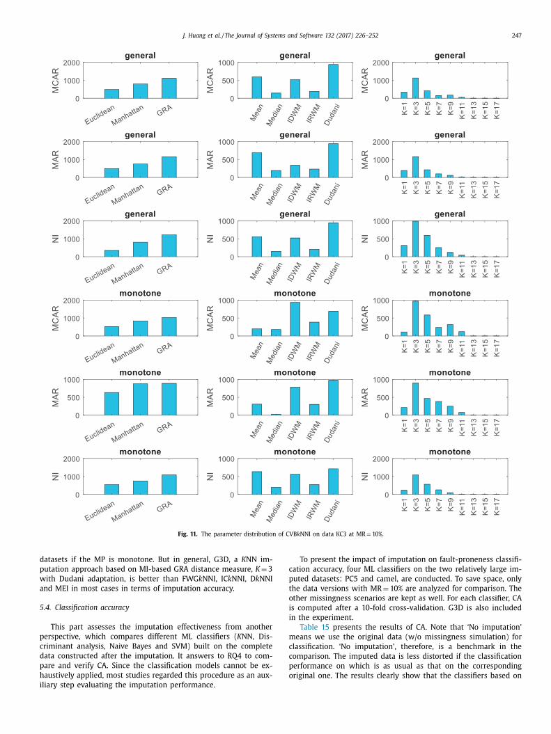
J. Huang et al. / The Journal of Systems and Software 132 (2017) 226–252 247
Fig. 11. The parameter distribution of CVB k NNI on data KC3 at MR = 10%.
d
p
w
a
5
p
c
d
p
h
i
c
p
t
o
i
i
m
c
c
p
o
atasets if the MP is monotone. But in general, G3D, a K NN im-
utation approach based on MI-based GRA distance measure, K = 3
ith Dudani adaptation, is better than FWG k NNI, IC k NNI, D k NNI
nd MEI in most cases in terms of imputation accuracy.
.4. Classification accuracy
This part assesses the imputation effectiveness from another
erspective, which compares different ML classifiers ( K NN, Dis-
riminant analysis, Naive Bayes and SVM) built on the complete
ata constructed after the imputation. It answers to RQ4 to com-
are and verify CA. Since the classification models cannot be ex-
austively applied, most studies regarded this procedure as an aux-
liary step evaluating the imputation performance.
To present the impact of imputation on fault-proneness classifi-
ation accuracy, four ML classifiers on the two relatively large im-
uted datasets: PC5 and camel, are conducted. To save space, only
he data versions with MR = 10% are analyzed for comparison. The
ther missingness scenarios are kept as well. For each classifier, CA
s computed after a 10-fold cross-validation. G3D is also included
n the experiment.
Table 15 presents the results of CA. Note that ‘No imputation’
eans we use the original data (w/o missingness simulation) for
lassification. ‘No imputation’, therefore, is a benchmark in the
omparison. The imputed data is less distorted if the classification
erformance on which is as usual as that on the corresponding
riginal one. The results clearly show that the classifiers based on

248 J. Huang et al. / The Journal of Systems and Software 132 (2017) 226–252
Table 15
The comparison of CA using different ML classifiers on data camel and PC5 with MR = 10%.
1 The maximum CAs in each condition are in green; the minimum CAs are in red; while the 2nd largest CAs are marked in blue.
r
f
u
q
p
a
p
c
H
o
t
E
e
(
(
i
v
m
B
T
either the original dataset or the incomplete one with MEI used
generally present relatively worse classification performance. In
terms of the CA after imputation, CVB k NNI and G3D are generally
superior to others in most cases. And the IC k NNI has a suboptimal
performance. In terms of the classifiers, K NN, Discriminant analy-
sis, and Naïve Bayes are more sensitive to imputation approaches
than SVM. The performance of SVM is even not sensitive to MM or
MP. In general, the results show that appropriate imputation ap-
proach could be beneficial to the CA of specific classifier. To sum,
when using CVB k NNI and G3D as the imputation approach on the
incomplete data, the classification bias could also be maintained or
even reduced in commonly used classification tasks.
6. Threats to validity
The threats to validity are generally distributed into four
groups: conclusion, internal, construct, and external validity. The
conclusion validity is related to the ability to draw significant cor-
rect conclusions; regarding which, we carefully applied the statis-
tical tests, showing statistical significance for the obtained results.
Moreover, we have used two relatively large datasets (camel and
PC5) to mitigate the threats related to the number of observations
composing the datasets.
The construct validity refers to the agreement between a theo-
etical concept and a specific measure. As to the evaluation of dif-
erent K nearest neighbor ( K NN) imputation approaches, we made
se of one balanced performance measure and 8 public software
uality datasets. The data repository used in the work has been
reviously used in numerous empirical quality studies.
As the study concentrates on a structural investigation of
novel K NN imputation approach, the internal validity on ex-
eriment design is presented in one aspect: CVB k NNI is a
omputation-consuming way to improve imputation accuracy.
owever, if the imputation accuracy is the top priority, the value
f CVB k NNI is then obvious. The proposal of G3D stands as an al-
ernative to mitigate this issue as well.
The threats to external validity are controlled well in this study.
ight object-oriented and procedural software quality datasets are
xamined in the study. Meanwhile, 3 missingness mechanisms
MMs), 2 missingness patterns (MPs), and 4 missingness ratios
MRs) are also considered during missingness simulation for test-
ng the performance of the proposed imputation approach under
arious conditions. One issue is that we did not consider adopting
ore different kinds of imputation approaches, for example, the
ayes multiple imputation (BMI), as the competitor to CVB k NNI.
his study only focuses on the improvement and comparison of
J. Huang et al. / The Journal of Systems and Software 132 (2017) 226–252 249
K
p
7
(
p
p
i
a
t
t
a
o
t
c
t
t
p
w
o
t
h
e
t
o
A
t
G
K
s
7
R
A
A
B
B
C
C
C
C
C
D
D
D
F
F
G
H
H
H
H
H
J
J
J
K
K
K
K
K
K
KL
L
L
L
L
L
M
M
M
M
NN related imputation approaches. In the future work, more com-
arison studies shall be explored.
. Conclusions and future work
This empirical study proposes a novel K Nearest Neighbor
K NN) based imputation approach: called CVB k NNI, and its im-
roved performance has been validated in the software quality
rediction domain. CVB k NNI is different to other approaches since
t does not have predetermined fixed estimator, and instead it
daptively selects the optimal estimator for each missing value in
he dataset. The estimator of CVB k NNI includes a pool of three dis-
ance measures, multiple choices of K values together with five
daptation methods. Our result shows that CVB k NNI outperforms
ther competing approaches in overall imputation accuracy. From
he returned estimator of the CVB k NNI, the optimal parameter
ombination of K NN imputation for software quality dataset is
hen correctly determined, which is named as G3D. Further evalua-
ions on the CVB k NNI have been performed, specifically on incom-
lete datasets and compared several other competing approaches.
In particular, 4 findings are noteworthy from the study:
(1) Our proposed cross-validation based K NN imputation could
further improve the imputation performance on software
quality datasets, in which calculating the feature relevance
during measuring the pair distance is very necessary.
(2) The impact of missingness mechanisms and patterns on
imputation performance exists. Non-ignorable missingness
mechanism could significantly impact the imputation accu-
racy. The impact of missingness pattern is related to the
dataset.
(3) The performance of fault-proneness classification is accept-
able when CVB k NNI was used as the preprocessing method.
(4) For K NN imputation using K = 3 and Dudani adaptation, to-
gether with the distance measure based on mutual infor-
mation weighted grey relational analysis, is considered ideal
and recommended for incomplete software quality datasets.
CVB k NNI could be easily applicable to other domains in soft-
are engineering, which are subject to further investigations in
ur future work. Theoretically it would further improve imputa-
ion accuracy when dealing with incomplete datasets, but also
elps to find the optimal K NN imputation algorithm under differ-
nt circumstance. Besides, determining more meaningful parame-
er configurations or components to further improve the accuracy
f CVB k NNI is also being investigated.
cknowledgement
The authors would like to thank the anonymous reviewers for
heir invaluable feedback. This work is supported in part by the
eneral Research Fund of the Research Grants Council of Hong
ong (No. 125113 , 1120 0 015 , 11208017 and 11214116 ), and the Re-
earch funds of City University of Hong Kong (No. 7004683 and
004474 ).
eferences
rcuri, A. , Briand, L. , 2014. A hitchhiker’s guide to statistical tests for assessing ran-
domized algorithms in software engineering. J. Softw. 24, 219–250 . zzeh, M. , 2012. A replicated assessment and comparison of adaptation techniques
for analogy-based effort estimation. Empir. Softw. Eng. 17, 90–127 . ansiya, J. , Davis, C.G. , 2002. A hierarchical model for object-oriented design quality
assessment. IEEE Trans. Softw. Eng. 28, 4–17 .
rás, L.P. , Menezes, J.C. , 2007. Improving cluster-based missing value estimation ofDNA microarray data. Biomol. Eng. 24, 273–282 .
artwright, M. , Shepperd, M.J. , Song, Q. , 2003. Dealing with missing software projectdata. In: 9th International Software Metrics Symposium (METRIC’03). Sydney,
Australia, pp. 154–165 .
aruana, R. , 2001. A non-parametric EM-style algorithm for imputing missing val-ues. The 4th International Conference of Artificial Intelligence and Statistics
(AISTATS’01) . hen, J. , Shao, J. , 20 0 0. Nearest neighbor imputation for survey data. J. Official Stat.
16, 113–132 . hidamber, S.R. , Kemerer, C.F. , 1994. A metrics suite for object oriented design. IEEE
Trans. Softw. Eng. 20, 476–493 . onversano, C. , Siciliano, R. , 2009. Incremental tree-based missing data imputation
with lexicographic ordering. J. Classif. 26, 361–379 .
eb, R. , Liew, A.W.-C. , 2016. Missing value imputation for the analysis of incompletetraffic accident data. Inf. Sci. 339, 274–289 .
uda, R.O. , Hart, P.E. , 1973. Pattern Classification and Scene Analysis. Wiley, NewYork .
udani, S.A. , 1976. The distance-weighted k-nearest-neighbor rule. IEEE Trans. Syst.Man Cybern. 325–327 .
inley, A.O. , McRoberts, R.E. , Ek, A.R. , 2006. Applying an efficient k-nearest neighbor
search to forest attribute imputation. Forest. Sci. 52, 130–135 . oss, T. , Stensrud, E. , Kitchenham, B. , Myrtveit, I. , 2003. A simulation study of the
model evaluation criterion MMRE. IEEE Trans. Softw. Eng. 29, 985–995 . arcía-Laencina, P.J. , Sancho-Gómez, J.-L. , Figueiras-Vidal, A.R. , Verleysen, M. , 2009.
K nearest neighbours with mutual information for simultaneous classificationand missing data imputation. Neurocomputing 72, 1483–1493 .
alstead, M.H. , 1977. Elements of Software Science (Operating and Programming
Systems Series). Elsevier Science Inc . enderson-Sellers, B. , 1996. Object-oriented metrics: Measures of Complexity. Pren-
tice-Hall, Inc . ron, K. , Templ, M. , Filzmoser, P. , 2010. Imputation of missing values for compo-
sitional data using classical and robust methods. Comput. Stat. Data Anal. 54,3095–3107 .
uang, C.-C. , Lee, H.-M. , 2004. A grey-based nearest neighbor approach for missing
attribute value prediction. Appl. Intell. 20, 239–252 . uang, J. , Li, Y.F. , Xie, M. , 2015. An empirical analysis of data preprocessing for ma-
chine learning-based software cost estimation. Inf. Softw. Technol. 67, 108–127 . ing, X.-Y. , Qi, F. , Wu, F. , Xu, B. , 2016. Missing data imputation based on low-rank
recovery and semi-supervised regression for software effort estimation. In: The38th International Conference on Software Engineering (ICSE’16). ACM, Austin,
TX, USA, pp. 607–618 .
önsson, P. , Wohlin, C. , 2006. Benchmarking k-nearest neighbour imputation withhomogeneous Likert data. Empir. Softw. Eng. 11, 463–489 .
ureczko, M. , Madeyski, L. , 2010. Towards identifying software project clusters withregard to defect prediction. In: The 6th International Conference on Predictive
Models in Software Engineering (PROMISE’10). ACM, Timisoara, Romania, p. 9 . hatibi Bardsiri, V. , Jawawi, D.N.A. , Hashim, S.Z.M. , Khatibi, E. , 2013. A PSO-based
model to increase the accuracy of software development effort estimation.
Softw. Qual. J. 21, 501–526 . hoshgoftaar, T.M. , Van Hulse, J. , 2008. Imputation techniques for multivariate miss-
ingness in software measurement data. Softw. Qual. J. 16, 563–600 . ocaguneli, E. , Member, S. , Menzies, T. , 2012a. Exploiting the essential assumptions
of analogy-based effort estimation. IEEE Trans. Softw. Eng. 38, 425–439 . ocaguneli, E. , Member, S. , Menzies, T. , 2012b. On the value of ensemble effort es-
timation. IEEE Trans. Softw. Eng. 38, 1403–1416 . ocaguneli, E. , Menzies, T. , Keung, J. , Cok, D. , Madachy, R. , 2013a. Active learning
and effort estimation: finding the essential content of software effort estimation
data. IEEE Trans. Softw. Eng. 39, 1040–1053 . ocaguneli, E. , Menzies, T. , Keung, J.W. , 2013b. Kernel methods for software effort
estimation: effects of different kernel functions and bandwidths on estimationaccuracy. Empir. Softw. Eng. 18, 1–24 .
ullback, S. , 1997. Information Theory and Statistics. Courier Corporation . all, U. , Sharma, A. , 1996. A nearest neighbor bootstrap for resampling hydrologic
time series. Water Resour. Res. 32, 679–693 .
i, D. , Deogun, J. , Spaulding, W. , Shuart, B. , 2004. Towards missing data imputation:a study of fuzzy k-means clustering method. In: The 4th International Confer-
ence of Rough Sets and Current Trends in Computing (RSCTC’04). Uppsala, Swe-den, pp. 573–579 .
i, J. , Al-Emran, A. , Ruhe, G. , 2007. Impact analysis of missing values on the pre-diction accuracy of analogy-based software effort estimation method AQUA. In:
The 1st International Symposium on Empirical Software Engineering and Mea-
surement (ESEM’07). Madrid, Spain, pp. 126–135 . i, Y.F. , Xie, M. , Goh, T.N. , 2009a. A study of mutual information based feature se-
lection for case based reasoning in software cost estimation. Expert Syst. Appl.36, 5921–5931 .
i, Y.F. , Xie, M. , Goh, T.N. , 2009b. A study of project selection and feature weightingfor analogy based software cost estimation. J. Syst. Softw. 82, 241–252 .
ittle, R.J. , Rubin, D.B. , 2002. Statistical Analysis With Missing Data. John Wiley &
Sons, Inc . a, X. , Zhong, Q. , 2016. Missing value imputation method for disaster decision-mak-
ing using K nearest neighbor. J. Appl. Stat. 43, 767–781 . agnussen, S. , Tomppo, E. , 2014. The k-nearest neighbor technique with local linear
regression. Scand. J. Forest Res. 29, 120–131 . aier, M. , Hein, M. , von Luxburg, U. , 2009. Optimal construction of k-nearest-neigh-
bor graphs for identifying noisy clusters. Theory Comput. Sci. 410, 1749–
1764 . air, C. , Kadoda, G. , Lefley, M. , Phalp, K. , Schofield, C. , Shepperd, M. , Webster, S. ,
20 0 0. Investigation of machine learning based prediction systems. J. Syst. Softw.53, 23–29 .

250 J. Huang et al. / The Journal of Systems and Software 132 (2017) 226–252
S
S
S
S
S
S
T
T
V
V
W
Z
Martin, R. , 1994. OO design quality metrics - An analysis of dependencies. In: The9th Annual Conference on Object-Oriented Programming Systems, Languages,
and Applications (OOPSLA’94). Portland, Oregon, USA, pp. 151–170 . McCabe, T.J. , 1976. A complexity measure. IEEE Trans. Softw. Eng. 2, 308–320 .
Mendes, E. , Watson, I. , Triggs, C. , Mosley, N. , Counsell, S. , 2003. A comparative studyof cost estimation models for web hypermedia applications. Empir. Softw. Eng.
8, 163–196 . Menzies, T., Krishna, R., Pryor, D., 2016. The PROMISE Repository of Empirical Soft-
ware Engineering Data. North Carolina State University, Department of Com-
puter Science http://openscience.us/repo . Minku, L.L. , Yao, X. , 2011. A principled evaluation of ensembles of learning machines
for software effort estimation. In: The 7th International Conference on Predic-tive Models in Software Engineering (PROMISE’11). Banff, Canada, pp. 1–10 .
Mittas, N. , Angelis, L. , 2010. LSEbA: least squares regression and estimation by anal-ogy in a semi-parametric model for software cost estimation. Empir. Softw. Eng.
15, 523–555 .
Mockus, A. , 2008. Missing Data in Software engineering, Guide to Advanced Empir-ical Software Engineering. Springer, pp. 185–200 .
Myrtveit, I. , Stensrud, E. , Olsson, U.H. , 2001. Analyzing data sets with missing data:an empirical evaluation of imputation methods and likelihood-based methods.
IEEE Trans. Softw. Eng. 27, 999–1013 . Pan, R. , Yang, T. , Cao, J. , Lu, K. , Zhang, Z. , 2015. Missing data imputation by K nearest
neighbours based on grey relational structure and mutual information. Appl.
Intell. 1–19 . Peng, H. , Long, F. , Ding, C. , 2005. Feature selection based on mutual information:
Criteria of max-dependency, max-relevance, and min-redundancy. IEEE Trans.Pattern Anal. Mach. Intell. 27, 1226–1238 .
Poloczek, J. , Treiber, N.A. , Kramer, O. , 2014. KNN regression as geo-imputationmethod for spatio-temporal wind data. In: International Joint Conference
SOCO’14-CISIS’14-ICEUTE’14. Springer, pp. 185–193 .
Rey-del-Castillo, P. , Cardeñosa, J. , 2012. Fuzzy min–max neural networks for cate-gorical data: application to missing data imputation. Neural Comput. Appl. 21,
1349–1362 . Sahri, Z. , Yusof, R. , Watada, J. , 2014. FINNIM: Iterative imputation of missing values
in dissolved gas analysis dataset. IEEE Trans. Ind. Inf. 10, 2093–2102 . Sarro, F. , Petrozziello, A. , Harman, M. , 2016. Multi-objective software effort estima-
tion. In: The 38th International Conference on Software Engineering (ICSE’16).
ACM, Austin, TX, USA, pp. 619–630 . Sentas, P. , Angelis, L. , 2006. Categorical missing data imputation for software cost
estimation by multinomial logistic regression. J. Syst. Softw. 79, 404–414 . Shepperd, M. , Schofield, C. , 1997. Estimating software project effort using analogies.
IEEE Trans. Softw. Eng. 23, 736–743 .
hepperd, M. , Song, Q. , Sun, Z. , Mair, C. , 2013. Data quality: some comments on theNASA software defect datasets. IEEE Trans. Softw. Eng. 39, 1208–1215 .
ilva-Ramírez, E.-L. , Pino-Mejías, R. , López-Coello, M. , 2015. Single imputation withmultilayer perceptron and multiple imputation combining multilayer percep-
tron and k-nearest neighbours for monotone patterns. Appl. Soft Comput. 29,65–74 .
ong, Q. , Shepperd, M. , 2007. A new imputation method for small software projectdata sets. J. Syst. Softw. 80, 51–62 .
ong, Q. , Shepperd, M. , Cartwright, M. , 2005. A short note on safest default miss-
ingness mechanism assumptions. Empir. Softw. Eng. 10, 235–243 . Song, Q. , Shepperd, M. , Chen, X. , Liu, J. , 2008. Can k-NN imputation improve the per-
formance of C4. 5 with small software project data sets? A comparative evalu-ation. J. Syst. Softw. 81, 2361–2370 .
tekhoven, D.J. , Bühlmann, P. , 2012. MissForest - non-parametric missing value im-putation for mixed-type data. Bioinformatics 28, 112–118 .
trike, K. , Emam, K.E. , Madhavji, N. , 2001. Software cost estimation with incomplete
data. IEEE Trans. Softw. Eng. 27, 890–908 . Suyundikov, A. , Stevens, J.R. , Corcoran, C. , Herrick, J. , Wolff, R.K. , Slattery, M.L. , 2015.
Accounting for dependence induced by weighted KNN imputation in pairedsamples, motivated by a colorectal cancer study. PLoS ONE 10, e0119876 .
royanskaya, O. , Cantor, M. , Sherlock, G. , Brown, P. , Hastie, T. , Tibshirani, R. , Bot-stein, D. , Altman, R.B. , 2001. Missing value estimation methods for DNA microar-
rays. Bioinformatics 17, 520–525 .
wala, B. , Cartwright, M. , Shepperd, M. , 2005. Comparison of various methods forhandling incomplete data in software engineering databases. In: The 2005 In-
ternational Symposium on Empirical Software Engineering (ISESE’05). NoosaHeads, Australia, pp. 105–114 .
aldiviezo, H.C. , Van Aelst, S. , 2015. Tree-based prediction on incomplete data usingimputation or surrogate decisions. Inf. Sci. 311, 163–181 .
an Buuren, S. , 2012. Flexible Imputation of Missing Data. CRC press .
Van Hulse, J. , Khoshgoftaar, T.M. , 2014. Incomplete-case nearest neighbor imputationin software measurement data. Inf. Sci. 259, 596–610 .
alkerden, F. , Jeffery, R. , 1999. Empirical study of analogy-based software effort es-timation. Empir. Softw. Eng. 4, 135–158 .
Zhang, S. , 2011. Shell-neighbor method and its application in missing data imputa-tion. Appl. Intell. 35, 123–133 .
hang, S. , 2012. Nearest neighbor selection for iteratively kNN imputation. J. Syst.
Softw. 85, 2541–2552 . Zhang, S. , Jin, Z. , Zhu, X. , 2011. Missing data imputation by utilizing information
within incomplete instances. J. Syst. Softw. 84, 452–459 . Zhang, S. , Li, X. , Zong, M. , Zhu, X. , Cheng, D. , 2017. Learning k for kNN Classification.
ACM Trans. Intell. Syst. Technol. 8, 1–19 .

J. Huang et al. / The Journal of Systems and Software 132 (2017) 226–252 251
artment of Computer Science at City University of Hong Kong, Hong Kong, China. He
ngineering and Engineering Management, City University of Hong Kong, and his B.Eng. onic Science and Technology of China. His research interests include mining software
learning.
Science from the University of Sydney, and his Ph.D. in Software Engineering from the
t Professor in the Department of Computer Science, City University of Hong Kong. His n, empirical modelling and evaluation of complex systems, and intensive data mining for
prestigious journals including IEEE-TSE, IEEE-SOFTWARE, EMSE and many other leading
artment of Computer Science at University College London, where she is member of the
are Engineering and Search Based Software Engineering (SBSE), with a particular interest anning, and app stores mining and analysis. She has published over 50 papers in top SE
IES award at GECCO 2016. She has served on more than 40 program committees and as 016, and been elected onto the steering committee for SSBSE in 2015. She has also been
editorial board of the Springer GPEM journal. Web page: http://www0.cs.ucl.ac.uk/staff/
trial Engineering at Tsinghua University, Beijing, China. In 2010, Dr. Li obtained his PhD esearch associate at the University of Tennessee in the same year. His research interests
n. He is the author of over 30 publications on peer-refereed international journals, such
Transactions on Power Systems and IEEE Transactions on Software Engineering. He is a international conferences on reliability and risk. He is a senior member of IEEE and a
eliability, risk and optimization at the undergraduate and master levels.
elbourne, Australia. He is an Associate Professor in the Department of Computer Science,
rests include software testing, e-commerce, and computers in education. His publications nal conferences, such as TOSEM, TSE, TRel, TSC, JSS, IST, Information Research, Computers
others. Dr. Yu is a past chair of the IEEE Hong Kong Section Computer Society Chapter.
es from The University of Hong Kong, Hong Kong. He is an Associate Professor in the
g Kong, Hong Kong. His current main research interests include program analysis and
lished extensively in venues such as TOSEM, TSE, TPDS, TSC, TRel, JSS, IST, STVR, CACM, , ICDCS, and others. Dr. Chan is the Special Issues Editor of the Journal of Systems and
Jianglin Huang is currently a postdoc fellow at the Dep
received his Ph.D. (2016) from Department of Systems E(2012) in Software Engineering from University of Electr
repository, software effort/quality estimation and machine
Jacky Wai Keung received his B.Sc. (Hons) in Computer
University of New South Wales, Australia. He is Assistanmain research area is in software effort and cost estimatio
software engineering datasets. He has published papers injournals and conferences.
Federica Sarro is a Senior Research Associate in the Dep
CREST centre. Her main research areas are Empirical Softwin software effort estimation, defect prediction, project pl
venues and won 4 international awards including the HUMthe program co-chair for SBSE at GECCO 2017 and SSBSE 2
guest editor for the IEEE TEVC journal and member of theF.Sarro/ .
Yan-Fu Li is a full professor at the Department of Indusat National University of Singapore and was a post-doc r
include system reliability, risk assessment and optimizatio
as IIE Transactions, IEEE Transactions on Reliability, IEEE member of the technical program committee of several
member of SRA. He is teaching three courses relevant to r
Y.T. Yu received the Ph.D. degree from The University of M
City University of Hong Kong, Hong Kong. His research intehave appeared in scholarly journals and leading internatio
and Education, ICSE, FSE, ISSRE, COMPSAC, QRS, ICCE, and
W. K. Chan received the B.Eng., M.Phil., and Ph.D. degre
Department of Computer Science, City University of Hon
testing for concurrent software and systems. He has pubComputer, ICSE, FSE, ISSTA, ASE, WWW, ISSRE, ICWS, QRS
Software.

252 J. Huang et al. / The Journal of Systems and Software 132 (2017) 226–252
1993) in Aalborg University in Denmark. He is currently an Associate Professor at the De-
ment, City University of Hong Kong. His teaching and research areas include management tegy, quality management, and international comparative study. He has published 100 ar-
he editorial board of International Journal of Technological Innovation, Entrepreneurship
lity and Reliability Management, and International Journal of Learning and Changes.
Hongyi Sun received his Ph.D. in Industrial Management (
partment of Systems Engineering and Engineering Manageof technological innovation, manufacturing/operations stra
ticles in international journals and conferences. He is in t
and Technology Management, International Journal of Qua