The Lattice-Boltzmann Method for Gaseous Phenomena

Xiaoming Wei1, Wei Li1, Klaus Mueller1 and Arie Kaufman1

Center for Visual Computing (CVC)

and Department of Computer Science

State University of New York at Stony Brook

Stony Brook, NY 11794-4400

Abstract

We present a physically-based, yet fast and simple method to simulate gaseous phenom-

ena. In our approach, the incompressible Navier-Stokes (NS) equations governing fluid motion

have been modeled in a novel way to achieve a realistic animation. We introduce the Lattice

Boltzmann Model (LBM) which simulates the microscopic movement of fluid particles by lin-

ear and local rules on a grid of cells, so that the macroscopic averaged properties obey the

desired NS equations. The LBM is defined on a 2D or 3D discrete lattice, which is used to

solve fluid animation based on different boundary conditions. The LBM simulation generates

1

in real-time an accurate velocity field and can incorporate an optional temperature field to ac-

count for the buoyancy force of hot gas. Because of the linear and regular operations on each

local cell of the LBM grid, we implement the computation in commodity texture hardware,

further improving the simulation speed. Finally, textured splats are used to add small scale tur-

bulent details, achieving high-quality real-time rendering. Our method can also simulate the

physically correct action of stationary or mobile obstacles on gaseous phenomena in real-time,

while still maintaining highly plausible visual details.

KEYWORDS Lattice Boltzmann Model, Graphics Hardware, GPU, Textured Splatting,

Gaseous Phenomena Modeling

1Email:wxiaomin,liwei,mueller,ari@cs.sunysb.edu

2

1 Introduction

Gaseous phenomena, such as rolling clouds, moving dust, rising steam and billowing smoke play

an important role in graphics simulations. A good fluid model for gaseous phenomena should

not only describe the flow, but also model the interaction between the flow and the surrounding

environment in a physically correct manner. In Computational Fluid Dynamics (CFD), fluid prop-

erties and behaviors have been studied for many years. However, while the goal of researchers in

fluid dynamics is to obtain a highly accurate fluid behavior, our goal is to achieve physically-based

realistic-looking results, while maintaining fast calculation and rendering speed.

A fluid is described by several macroscopic variables, such as density, velocity, pressure, and

temperature. In CFD, fluid dynamics can be described by the Navier-Stokes (NS) equations. The

following formulas are the incompressible 3D NS equations,

∇ ·u = 0 (1)

∂u∂t

=−(u·∇)u− 1ρ

∇p+ν∇2u+ f (2)

whereu is the velocity field,p is the pressure field,ν is the kinematics viscosity of the fluid,ρ

is its density,f is an external force, and∇ is the vector of spatial partial derivatives. Equation 1

describes the conservation of mass, indicating that the inflow and outflow of mass in a fluid element

are balanced. Equation 2 shows the conservation of momentum. It describes the velocity changes

in time, due to convection, spatial variations in pressure, viscous forces, and external forces. Many

books and articles [12, 16] have been published on how to solve these equations numerically. The

difficulty in solving the NS equations is due to their nonlinear terms. This complexity makes the

solution of these equations in 3D very time-consuming.

3

Since our goal is to achieve real-time computation and rendering speed, we propose in this

paper the use of the linear and microscopic Lattice Boltzmann Model (LBM), instead of solving the

macroscopic NS equations directly. Fluid flow consists of many tiny flow particles. The collective

behavior of these microscopic particles results in the macroscopic dynamics of the fluid. The LBM

is originated from a cellular automata representing individual particle packets moving on a discrete

lattice at discrete time steps. The calculation is performed on a regular grid. At every grid cell,

there are variables indicating its status. All the cells modify their status at every time step based

on the same linear and local rules. Since these interaction rules are defined in such a way that

they satisfy the conservation of mass and momentum at each local grid cell, the macroscopic NS

equations are satisfied globally. The LBM also helps us handle the boundary conditions and the

interaction of the gaseous phenomena with the environment in a physically correct way.

In the traditional CFD approach, the physical modeling of the fluid behavior and the numerical

approximation are separate steps, while in LBM, those two phases are combined together. The

main difference between the LBM and the traditional numerical approaches of the NS equations

is that in the LBM the physical transition rules are discrete, while in the latter the discretization

is performed on the level of the macroscopic NS equations. In both cases, the same physical

conservation laws are satisfied.

In this paper, we show the application of the LBM to model both the movement of gaseous phe-

nomena and their behavior with stationary or moving obstacles at interactive frame rates. The final

performance gap is filled by realizing that the linear and local calculations that occur at each grid

cell are very amenable to acceleration on commodity graphics hardware, resulting in interactive

4

modeling rates of 30 frames/sec.

Using the LBM to yield a velocity volume rich in small scale rotational and turbulent details

still requires a large 3D grid. Since our goal is to achieve fluid-like effects in real-time, and not

a strict physical simulation, we base our work on relatively low-resolution grids. Texture hard-

ware acceleration enables us to accomplish real-time computation speed. To provide the missing

details, we augment the low-resolution velocity field with high-resolution textures of small-scale

perturbations, which can also be efficiently rendered on commodity texture mapping hardware.

Our two-tier approach is justified by the fact that in most graphics applications gaseous objects

are mainly used to enhance the realism of the virtual environment - users don’t require to observe

highly-accurate details of the interaction between gaseous phenomena and obstacles. All that is

needed is that the gases are behaving in a near physically correct way. It turns out that by com-

bining a low-resolution velocity grid with high-detailed textures a surprisingly realistic viewing

experience can be generated. By incorporating into the LBM a number of physically-accurate ef-

fects, such as the buoyancy effect of hot gases, additional realism can be provided. Our framework

makes efficient use of the concept of textured splats [6], which are associated with the macro-

scopic particles to represent the gaseous phenomena. The textured splats form the observable

”display particles”, such as the smoke particles or dust particles, while the LBM deals with non-

observable microscopic particles. To distinguish the two, we use the term ”packet” to stand for

the microscopic particles and the term ”display primitive” to stand for the smoke or gas particles.

The display primitives move freely through space, subjected to the velocity field simulated by the

underlying LBM grid as well as to other forces, such as the temperature-induced buoyancy.

5

The rest of the paper is organized as follows. In the next section, we briefly discuss related work

in computer graphics on gaseous phenomena modeling and manipulation. In Sections 3 and 4, we

present the basic ideas of the LBM and the initial and boundary condition settings. In Section 5, we

discuss the incorporation of a temperature field in the LBM. We introduce the implementation of

the LBM calculation in texture hardware in Section 6. In Section 7, we show how to use textured

splatting to achieve high-quality real-time rendering speed. Finally, we outline our implementation

and describe several examples in Section 8.

2 Previous Work

A common approach to simulating gaseous phenomena is procedural modeling [11, 27, 31], where

fluid behaviors are described by procedural functions. This method is fast and easy to program,

but it is difficult to find the proper parameter settings that achieve realistic results. The interactions

between the fluid and the surrounding objects, such as flowing around obstacles, blown by the

wind, are also difficult to model in a physically correct manner.

Physically-based modeling is another broadly used method; however, it usually requires a large

amount of computation time and memory, especially in 3D. In 1991, Wejchert and Haumann [39]

gave an analytic solution to the NS equations by using simple flow primitives. Chen and Lobo

[2] solved a simplified NS equations in 2D using a finite difference approach. Later, Foster and

Metaxas [14] presented a full 3D finite difference solution to simulate the turbulent rotational

motion of gas. Because of the inherent instability of the finite difference method with a larger time

step, the speed of this approach is limited. Stam [32] devised a fluid solver using semi-Lagrangian

advection scheme and implicit solver for the NS equations. Each term of the equations is handled

6

in turn starting with external force, then advection, diffusion and finishing with a projection step.

This method is unconditionally stable and produces compelling simulations of turbulent flows. It

can also achieve real-time speed for a low-resolution grid. However, the numerical dissipation

associated with the method causes the turbulence to decay too rapidly. Fedkiw et al. [13] further

improved the result by introducing the concept of vortex confinement to the graphics field. The

problem of numeric dissipation is addressed by feeding energy back into vortices through vortex

confinement. Two rendering approaches were used in their work: one is a fast hardware based

renderer; the other is a expensive photon map renderer to create production quality animations.

In this paper, we demonstrate a new and pioneering direction on how real-time fluid simula-

tion could also be approached, instead of solving the traditional NS equations. All of the above

methods generate fluid-like behaviors by solving macroscopic equations either by explicit or im-

plicit approaches. In contrast, the LBM approach considers the problem from the microscopic

perspective. Since we use the LBM on a relatively low-resolution grid, one may ask why not solve

the NS equations on the same grid. Although it is true that combining the NS equations with the

high-resolution textures has the same effect, however, the computation of the NS equations is not

as simple as that of the LBM. Also, the fact that the calculation of the LBM only consists of simple

operations such as addition, subtraction and multiplication, and it is conducted locally, it allows us

to further improve the calculation speed of LBM by employing commodity texture hardware. This

achieves the desired real-time speed. In the next section, we present a complete framework for

the LBM-based fluid simulation and how its calculation is implemented based on the fast growing

GPU technology.

7

Physically-based particle models [5, 7, 22, 24, 34, 35, 36] have also been used to describe fluid

behaviors. Particle systems were first introduced by Reeves [29] as a technique for modeling fuzzy

objects, such as fire, clouds, smoke and water. Tonnesen [36] used a discrete model for the heat

transfer equations to describe the interaction of particles due to the thermal energy. Terzopoulos

et al. [35] implemented a similar approach. Particles and springs are utilized to render a series of

”blobbies” . Desbrun and Gascue [7, 8] developed a paradigm extended from the Smoothed Particle

Hydrodynamics approach used by physicists for cosmological fluid simulation. This technique

defines a type of particle system which uses smoothed particles as samples of mass smeared out

in space. A highly inelastic fluid is simulated by computing the variations of continuous functions

such as mass density, speed, pressure, or temperature over space and time. Stora et al. [34] also

used smooth particles to simulate lava flow. Particles are coated with implicit surfaces to get the

final rendering result. Particles in all of the above methods move and interact freely in space. They

are irregular, difficult and expensive to track atO(N2) complexity. While, in the LBM approach,

particle packets move and interact on a regular grid based on linear and local rules and it is proved

that the global behavior is the same as the one achieved by directly solving the heavy NS equations

(which is what is mostly done in graphics).

Dobashi et al. [9] implemented a realistic animation of clouds based on the cellular automata

model proposed by Nagel and Raschke [26]. Our work is fundamentally different from theirs.

Nagel’s model can only be used to model clouds. In contrast, the LBM is a general method used

to describe a variety of fluids. Harris et al. [18] implemented coupled map lattice, a variation of

cellular automata, on graphics hardware, which has similar motivation as this paper. To the best of

8

our knowledge, we pioneered the introduction and use of the LBM to simulate gaseous phenomena

in the graphics literature.

3 Lattice Boltzmann Model

The LBM [19, 25] is a lattice model originated in cellular automata. It is defined on a 2D or

3D discrete grid, where the time and the state of each cell are also discrete. Fluid behavior can

be understood as a self-organizing process evolving from the microscopic collisions of atoms or

molecules. Cellular automata is used to simulate these microscopic movements and collisions in

order to get the continuum macroscopic equations of fluid dynamics in two and three dimensions.

The class of cellular automata used for the simulation of fluid dynamics is called theLattice Gas

Automata(LGA) [10]. The main difference between the LGA and the traditional numerical ap-

proaches of the NS equations is that in the LGA the physical evolution rules are discrete, while in

the latter the discretization is performed on the level of the macroscopic flow equations.

The first LGA, introduced by Hardy, Pazzis and Pomreau, was called the HPP model, defined

on a square lattice [17]. In this model, microscopic particles of unit mass and unit speed move along

the lattice links. Not more than one particle in a given direction can be found at a given time and

node. When two microscopic particles arrive at a node from opposite directions, they immediately

leave the node in the two other, previously unoccupied directions. These rules conserve mass

(particle number) and momentum. The main problem with this model is that the gaseous behavior

it modeled is not isotropic.

A historically important lattice gas model is the FHP model, introduced by Frisch, Hasslacher

and Pomeau [15] in 1986. It is a 2D hexagonal lattice used to ensure macroscopic isotropy. In

9

this model, each cell has six nearest neighbors and consequently six possible velocity directions.

Updating the grid involves two types of rules: propagation and collision. Propagation means the

microscopic particles will move to the nearest neighbor along their velocity direction. Collision is

the most important part. It can force particles to change directions, and is decided by the collision

operator. No matter how we define the collision operator, the conservation of mass and momentum

must be satisfied. For instance, when two microscopic particles enter the same node with opposite

velocities, both of them are deflected by 60 degrees, such that the net momentum in the post

collision state remains zero. When multiple states are possible, a random selection is made. Figure

1 represents the collision rules for the FHP model.

Figure 1: Collision rules of the FHP model, defined on a triangular lattice. An arrow denotes amicroscopic particle and its moving direction. When multiple post collision states are possible, arandom selection is made. The collision rules satisfy mass and momentum conservation.

It can be demonstrated [15] that by observing the propagation and collision rules, we can

simulate the following macroscopic equations based on the LGA:

∂u∂t

=−(g(ρ)u·∇)u− 1ρ

∇p+ν∇2u (3)

whereρ is the density and can be calculated as the average number of microscopic particles per cell

andg(ρ) = ρ−3ρ−6. If we renormalize the timet, the viscosityν and the pressurep usingt

′= g(ρ)t,

ν′ = νg(ρ) , p

′= p

g(ρ) , the NS equations for incompressible fluids without external force can be

recovered.

10

Although the LGA has proven to be very useful for modeling fluid behavior, one major draw-

back of the method is the statistical noise in the computed hydrodynamic fields. This is a direct

consequence of the single particle Boolean operation. One method to smooth out the noise is to

average in space and time. In practice, spatial averages can be taken over 64, 256, 512 or 1024

neighboring cells for time-dependent flow in two dimensions. This, however, dramatically limits

the space resolution we can get. The problem can be solved by replacing the Booleans in the LGA

model byreal-valued densitiesof microscopic particles that move along each bond of the lattice,

following the motion of anaveragedistribution fqi of microscopic particles. This gives rise to a

model known as theLattice Boltzmann model (LBM)[3]. In the densitiesfqi, the indexqi describes

the D-dimensional sub-lattice defined by the permutations of (±1,...,±1,0,...0) whereq is the num-

ber of non-zero components andi counts the sub-lattice vectors. For a 2D LBM, there are three

lattice models: D2Q5, D2Q7 and D2Q9. Since our goal is to simulate the 3D gaseous phenomena,

we concentrate on the 3D LBM. For a 3D grid, the geometry of the model should be symmetrical

to satisfy the isotropic requirement of fluid properties. To correctly recover the NS equations, it

also requires sufficient lattice symmetry. In order to understand the design of 3D LBM model, the

notion ofsub-latticeis used in the LBM literature. Out of the 26 neighbors of an individual cell,

four symmetrical sub-lattices are defined on a 3D grid, as described in Figure 2 (a)-(d):

(a) q=0, the cell (0,0,0) has particle packets with zero velocities;

(b) q=1, the six nearest neighbors(±1,0,0),(0,±1,0), (0,0,±1), where the particle packets

move with unit velocity;

(c) q=2, the twelve second-nearest neighbors(±1,±1,0), (0,±1,±1), (±1,0,±1), where the

11

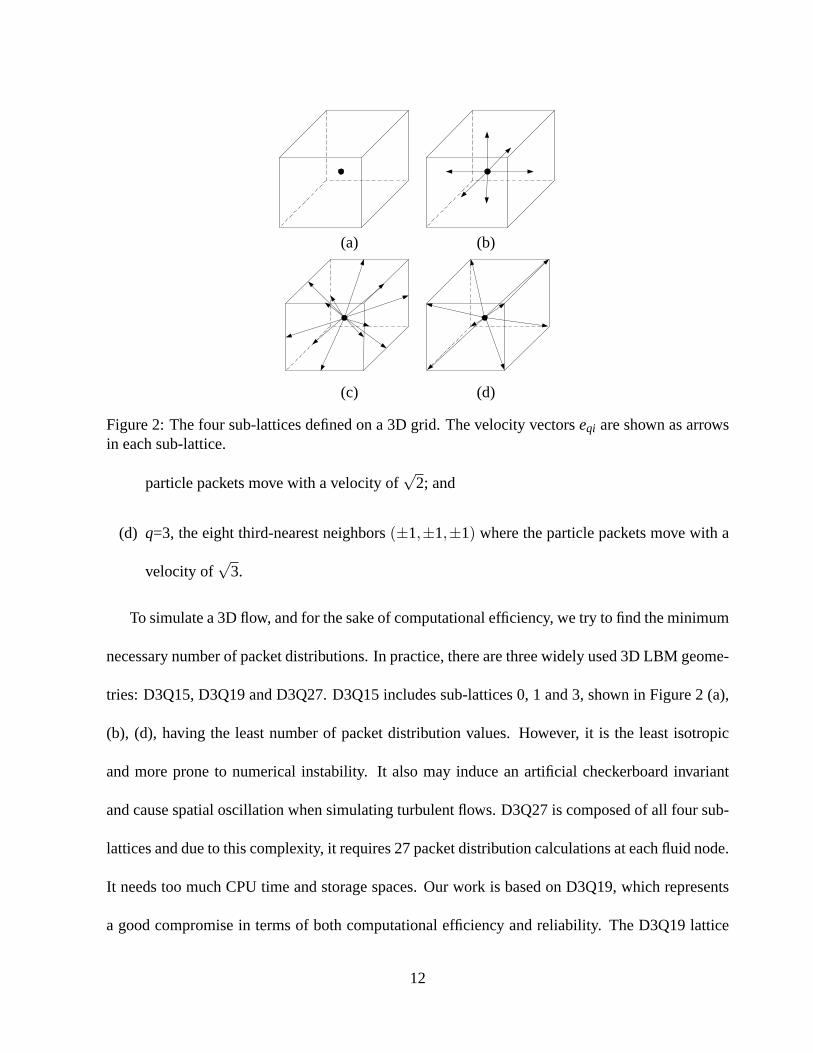
(a) (b)

(c) (d)

Figure 2: The four sub-lattices defined on a 3D grid. The velocity vectorseqi are shown as arrowsin each sub-lattice.

particle packets move with a velocity of√

2; and

(d) q=3, the eight third-nearest neighbors(±1,±1,±1) where the particle packets move with a

velocity of√

3.

To simulate a 3D flow, and for the sake of computational efficiency, we try to find the minimum

necessary number of packet distributions. In practice, there are three widely used 3D LBM geome-

tries: D3Q15, D3Q19 and D3Q27. D3Q15 includes sub-lattices 0, 1 and 3, shown in Figure 2 (a),

(b), (d), having the least number of packet distribution values. However, it is the least isotropic

and more prone to numerical instability. It also may induce an artificial checkerboard invariant

and cause spatial oscillation when simulating turbulent flows. D3Q27 is composed of all four sub-

lattices and due to this complexity, it requires 27 packet distribution calculations at each fluid node.

It needs too much CPU time and storage spaces. Our work is based on D3Q19, which represents

a good compromise in terms of both computational efficiency and reliability. The D3Q19 lattice

12

Figure 3: The D3Q19 lattice geometry

consists of three sub-lattices: sub-lattices 0, 1 and 2, shown in Figure 2 (a)-(c). In other words, at

each cell of D3Q19, there are 19 possible flow directions and thatfm(x, t) is the packet distribution

at locationx, at timet and moving in directionm, where1≤m≤ 19. Figure 3 shows the D3Q19

model lattice geometry. The velocity directions of the 18 moving packet distributions are shown

as arrows. The center is the packet distribution with zero velocity.

Similar to the LGA, the LBM updates the packet distribution values at each node based on two

simple and local rules: collision and propagation. Collision describes the redistribution of particle

packets at each local node. It is decided by the collision operator. Propagation means the particle

packets move to the nearest neighbor along their velocity directions. These two rules of the LBM

can be described by the following equations:

collision : f newqi (x, t)− fqi(x, t) = Ωqi (4)

propagation: fqi(x+eqi, t +1) = f newqi (x, t) (5)

whereΩ is a general collision operator andeqi is the unit vector, representing the packet velocity

along the lattice link. The collisions are completely local, making the LBM efficiently paralleliz-

13

able. In one time stept, each packet distribution value at every node is updated based on the

collision operatorΩ. Then, in time stept+1, the new packet distribution value propagates to the

nearest node along the velocity vectoreqi.

The macroscopic density (mass)ρ and velocityu are calculated from the respective velocity

moments of the packet distributions as follows:

ρ = ∑qi

fqi (6)

u =1ρ ∑

qifqieqi (7)

Combining Equations 4 and 5, we getfqi(x+ eqi, t + 1)− fqi(x, t) = Ωqi. The update of the

LBM system is decided by the collision operator. It is critical to selectΩqi in such a way that

the mass and momentum are conserved locally. Based on the work of Chen and Doolean [3],

we assume that for each individual packet distributionfqi at each cell, there is always a local

equilibrium packet distributionf eqqi . Its value only depends on the conserved quantitiesρ andu at

that cell. In this way, we get a new equation, also called thekinetic equation:

fqi(x+eqi, t +1)− fqi(x, t) =−1τ( fqi(x, t)− f eq

qi (ρ,u)) (8)

whereτ is the relaxation time scale andf eqqi (ρ,u) is the equilibrium packet distribution. According

to Muders’s work [25], the equilibrium packet distribution can be represented by a linear formula:

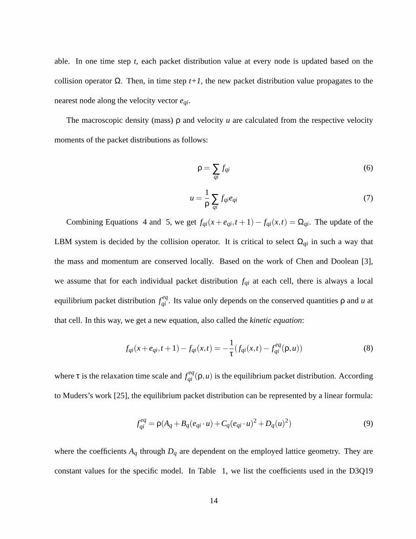
f eqqi = ρ(Aq +Bq(eqi ·u)+Cq(eqi ·u)2 +Dq(u)2) (9)

where the coefficientsAq throughDq are dependent on the employed lattice geometry. They are

constant values for the specific model. In Table 1, we list the coefficients used in the D3Q19

14

model. Using these coefficients in conjunction with Equations 8 and 9 ensures local conservation

of mass and momentum.

Table 1: Coefficients of the three sub-lattices in the D3Q19 model

Sub-lattice 0 Sub-lattice 1 Sub-lattice 2Aq

13

118

136

Bq 0 16

112

Cq 0 14

18

Dq −12 − 1

12 − 124

Theviscosityof a fluid is a measure of the fluid resistance to change of shape. For example,

water has a higher viscosity value than gas. In LBM, the viscosityν is decided by the parameterτ

with equationν = 13(τ− 1

2). Since the viscosity is always greater than zero,τ must be greater than

12.

Our algorithm for calculating the LBM is as follows:

1. Set the initial conditions for all grid cells, choose proper density and velocity for inlet cells,

and select a relaxation time scaleτ;

2. Calculate the macroscopic variables of density and velocity for each cell using Equations 6

and 7;

3. Compute the equilibrium packet distribution for each packet distribution by Equation 9;

4. Plug the packet distribution and equilibrium values into the kinetic Equation 8;

5. Propagate the packet distribution to all neighboring cells;

6. Modify the packet distribution locally to satisfy the boundary conditions;

15

7. Back to Step 2.

4 Initial and Boundary Conditions

Initial conditions are usually specified in terms of macroscopic variables, such as densities and ve-

locities. For the LBM, these macroscopic values are translated into the corresponding microscopic

packet distribution values for each fluid node. This is done by solving the equilibrium Equation 9.

Hence, the initial values of the density and velocity of each node are plugged into Equation 9, and

the equilibrium particle distribution values are set as the initial packet distribution values for each

node.

For a grid node near the boundary, some of its neighboring nodes lie outside the fluid domain.

Therefore, the packet distribution values at these nodes are not uniquely defined. For D3Q19, as

shown in Figure 4, there are several unknown packet distribution values for the boundary nodes,

for example, five unknowns for planar surface nodes and nine for concave-edge nodes. We need to

generate a boundary solution to set these unknown values.

Different types of boundary conditions have been introduced in the field of Hydrodynamics for

the LBM. Bounce-back is the simplest one, where boundary nodes are placed half-way between the

grid points. When particle packets propagate to the boundary nodes, they just bounce back along

the same link. The propagation step is changed tof−qi(x, t +1) = fqi(x, t). Another approach is us-

ing periodic boundary conditions. Here, the departing packet distribution along outward-pointing

links is allowed to re-enter the lattice via corresponding inward-pointing links on opposite bound-

aries. Both of these approaches are easy to implement and solve the unknown packet distribution

values based on the known packet distribution values of the neighboring cells. However, these two

16

(a) (b)

Figure 4: Boundary geometry examples for D3Q19: (a) planar boundary surface with five unknownvalues, (b) concave edge boundary node with nine unknown values (some invisible links shown bydashed arrow lines).

methods cannot set a unique value for the invisible links shown in Figure 4(b). Also, they can’t be

used to set the specific density and velocity constraints at the inlets, outlets and walls.

The purpose of setting boundary conditions is to determine the packet distribution values for the

incoming links on the boundary nodes. Most methods [19], such as the bounce-back and periodic

boundary condition, calculate these unknown packet distribution values explicitly. In this way,

we cannot determine the velocity and density value on these boundary nodes, such as a velocity

value of0.1 at the inlet boundary node. An incorrect density or velocity value at the boundary

nodes can eventually cause a negative density value at local grid points. As we solve the kinetic

Equation 8 withτ close to12, we find that if f eq

qi (ρ,u) is much smaller thanfqi(x, t), the packet

distribution valuefqi(x+eqi, t +1) will be changed to a negative number, which is incorrect. This

error can accumulate and eventually generate a negative density value. The problem can happen as

the boundary conditions become complicated, such as a fast moving boundary object or a complex

geometric structure.

In our work, we implemented the boundary conditions based on Mei et al.’s method [23] for

curved boundaries. In Mei et al.’s approach, the problem is solved in another way. Instead of

17

fluid node ff

fluid node f

boundary node b

wall boundary

qi e

qi e

w

Figure 5: The 2D projection of a regularly spaced lattice and a wall boundary.eqi andeqi arevelocity vectors in opposite directions.

directly setting the microscopic values, they calculate the macroscopic variables of density and

velocity at the boundary nodes first. By modifying the equilibrium equation, one can get better

results for complicated boundaries.

As shown in Figure 5, in the propagation step, the knowledge offqi(xb, t) of a nodeb at xb on

the boundary side is required in order to obtain thefqi(xf , t +1) for a nodef atxf on the fluid side.

To decide thefqi(xb, t), we define

δ =|xf −xw||xf −xb|

(10)

as the fraction of an intersected link in the fluid region, (it is obvious that0≤ δ≤ 1). The fqi(xb, t)

is calculated based on the packet distribution values, velocity and density values of neighboring

cells at the current time step:

fqi(xb, t) = (1−χ) fqi(xf , t)+χ f ∗qi(xb, t)+6Aqρeqi ·uw (11)

whereAq is the constant value we introduced in Equation 9.χ is defined byδ andτ (see below),

anduw indicates the speed of the wall boundary. In the case of boundary surfaces with nonzero

18

velocity, we modify the value ofuw. f ∗qi(xb, t) is the packet distribution value at the boundary node

b. It is decided by a modified equilibrium distribution function:

f ∗qi(xb, t) = ρ(Aq +Bqeqi ·ub f +Cq(eqi ·uf )2−Dq(uf )2) (12)

whereAq, Bq, Cq andDq are the constant coefficients defined in Equation 9, andub f is the virtual

speed at the boundary nodeb. It is set according toδ. Whenδ≥ 1/2, we defineχ = 2δ−1τ+1/2, and

ub f = (1− 32δ

)uf +32δ

uw (13)

Whenδ < 1/2, we haveχ = 2δ−1τ−2 and :

ub f = uf f (14)

5 Temperature Field

In this section, we show how to incorporate a temperature field to model the buoyancy force of

hot gases. Other types of external forces can also be added based on the work of Muders [25].

The temperature of smoke or gas has a direct effect on the behavior of their motion. Hot smoke

tends to rise more quickly due to the buoyancy effect. The D3Q19 model used in our work is an

isothermal model and it can’t describe the energy transfer due to difference in temperature. There

are also many thermal LBMs [3] in the Hydrodynamics field. However, most of them suffer from

instability problems.

To describe the effect of the buoyancy force, the evolution of temperature must also be modeled.

The change of the temperature of the smoke in the air can be characterized as a combination of

the convection and diffusion of heat in neighboring cells. To achieve fast speed, we use a linear

19

equation, similar to [4], instead of an accurate differential equation, to approximate the change of

temperature for the display primitives. Our model is governed by the following heat formula:

Tk(t) = αTk(t−1)+β ∑j 6=k

G(dk j)Tj(t−1) (15)

whereα is the conservation coefficient,β is the transferability coefficient,dk j is the distance be-

tween the display primitivek and j, andG() is a function describing the thermal diffusion. We

use a Gaussian filter as the functionG() to approximate the effect of diffusion. Att=0, Tk(0) is a

predefined initial value, indicating the initial temperature of the display primitives.

If the temperature of a particle is lower than the ambient temperature in the air, the particle will

disappear. For each particle, we add the vertical buoyancy force to the movement of the particle.

This force depends on the temperature field and is governed by the following equation:

Fbuoyancy= Hg(Tk−Tambient) (16)

whereg is the gravity in the vertical direction,H is the coefficient of thermal expansion, and

Tambient is the predefined ambient temperature value.

6 Mapping LBM to Graphics Hardware

We briefly review in this section the basic ideas of mapping LBM to graphics hardware, that is,

a graphics processing unit (GPU). (For more details see [21].) To compute the LBM equations

on graphics hardware, we divide the LBM grid and group the packet distributionsfqi into arrays

according to their velocity directions. All the packet distributions with the same velocity direction

are grouped into the same array, while keeping the neighboring relationship of the original model.

Figure 6 shows the division of a 2D model. We then store the arrays as 2D textures. For a 2D

20

Figure 6: Division of the D2Q9 model. Distribution values are grouped according to their velocitydirections.

model, all such arrays are naturally 2D, while for a 3D model, each array forms a volume and is

stored as a stack of 2D textures. The idea of the stack of 2D textures is from 2D texture-based

volume rendering, but note that we don’t need three replicated copies of the dataset.

In addition to the packet distributions, the densityρ, the velocityu, and the equilibrium distri-

butions f eqqi are stored similarly in 2D textures. We project multiple textured rectangles with the

color-encoded densities, velocities and distributions. For convenience, the rectangles are parallel

to the viewing plane and are rendered orthogonally. By setting the texture interpolation to nearest-

neighbor, and choosing the resolution of the frame buffer and the texture coordinates properly, we

create a one-to-one mapping from the texture space to the image space (one texel mapped to one

pixel).

The textures of the packet distributions are the inputs. Density and velocity are then computed

from the distribution textures. Next, the equilibrium distribution textures are obtained from the

densities and the velocities. According to the propagation equation, new distributions are computed

from the distributions and the equilibrium distributions. Finally, we apply the boundary conditions

and update the distribution textures. The updated distribution textures are then used as inputs for

the next simulation step. To reduce the overhead of switching between textures, we stitch multiple

21

textures representing packet distributions with the same velocity direction into one larger texture.

Figure 7 shows an example, in which, every four slices are stitched into a larger texture.

According to Equation 5, each packet distribution having non-zero velocity propagates to the

neighboring grid every time step. Since we group packets based on their velocity directions, the

propagation is accomplished by shifting distribution textures in the direction of the associated ve-

locity. We decompose the velocity into two parts, the velocity component within the slice (in-slice

velocity) and the velocity component orthogonal to the slice (orthogonal velocity). The propaga-

tion is done for the two velocity components independently. To propagate in the direction of the

in-slice velocity, we simply translate the texture of distributions appropriately.

If we don’t stitch multiple slices into one texture, the propagation in the direction of the or-

thogonal velocity is done simply by renumbering the distribution textures. Because of the stitch-

ing, we need to apply translation inside the stitched textures as well as copying sub-textures to

other stitched textures. Figure 7 shows the out-of-slice propagation for stitched slices. The in-

dexed blocks denote the slices storing packet distributions. The rectangles in thicker lines mark the

sub-textures that are propagated. For example, the sub-texture composed of slices 1 to 3 is shifted

down by the size of one slice in the Y dimension. Slices 4 and 8 are moved to the next textures.

Note that in time stept +1, a new slice is added owing to the inlet or the boundary condition, while

a block (12) has moved out of the framework and is discarded.

To implement the LBM computation with graphics hardware, we need to map all the variables

to the range of [0, 1] or [-1, 1]. Special care must be taken so that all the intermediate values

are also within the hardware supported range. Because various multiplications involved, we only

22

Figure 7: Propagation of the packet distributions along the direction of the velocity componentorthogonal to the slices.

apply scaling to change the numerical ranges. Apparently, the scale factors should be appropriate

so that no clamping error occurs and the computation exploits the full precision of the hardware.

For each functiony(x), we compute two scaling factors: the left-hand scalarymax= maxx(|y(x)|),

and the right-hand scalarU(y) as the maximal absolute value of all intermediate results during the

evaluation ofy(x), no matter what computation order is taken when the computation contains mul-

tiple operations. Assumef maxq is the left-hand scalar of the packet distributions and the equilibrium

packet distributions of sub-latticeq. We define the scaled distributionsfqi and the scaled densityρ

as:

fqi =1

f maxq

fqi (17)

ρ =ρ

ρmax = ∑qi

f maxq

ρmax fqi (18)

23

Since all thefqi are positive inputs,ρmax= U(ρ) = ∑qi f maxq . We also define:

1ρ′

=ρmin

ρρmax (19)

whereρmin is the lower bound of the density and1ρ′ ∈ [0,1].

We compute the right-hand scalar of the velocityU(u) as:

U(u) =1

ρmin maxb

∑qi

f maxq eqi[b] > 0 (20)

whereb is the dimension index of vectoreqi. Note thatU(u) andumaxare scalars instead of vectors.

Then, the scaled velocity is computed as:

u =u

umax =U(u)umax

1ρ′ ∑qi

(f maxq

U(u)ρmineqi) fqi (21)

With such range scaling, Equations 8 and 9 become:

fqi(x+eqi, t +1) = fqi(x, t)− 1τ( fqi(x, t)− f eq

qi ) (22)

f eqqi =

U( f eqq )

f maxq

ρ(Aqρmax

U( f eqq )

+2Bqumaxρmax

U( f eqq )

<eqi

2, u > +

4Cq(umax)2ρmax

U( f eqq )

<eqi

2, u >2 +

4Dq(umax)2ρmax

U( f eqq )

<u2,u2

>) (23)

For D3Q19 model,Aq≥ 0, Bq≥ 0, Cq≥ 0 andDq≤ 0, hence:

U( f eqqi ) = max((ρmaxAq +2Bqumaxρmax+4Cq(umax)2ρmax),(2Bqumaxρmax−4Dq(umax)2ρmax))(24)

Note that in Equation 23, we scaled the vectors before the dot products. The scaling factor is

chosen to be a power of two for easy implementation in hardware.

24

A major concern about using graphics hardware for general computation is accuracy. Most

graphics hardware supports only 8 bits per color channel. Fortunately, the variables of the LBM

fall into a small numerical range which makes the range scaling effective. Besides, the property of

the LBM, that the macroscopic dynamics is insensitive to the underlying details of the microscopic

physics [1], relaxes the requirement on the accuracy of the computation. In the new generation of

GPUs, such as ATI’s R300 and Nvidia’s NV30, floating point computation is available throughout

the fragment shader, hence the accuracy is less an issue. However, floating point requires more

memory and is slower than its fixed-point counterpart. Therefore, the proposed scaling is still

valuable in applications where speed is more important than accuracy, or the variables are restricted

to a small range. Note that our range scaling makes no assumption of the precision of the hardware.

7 Rendering with Textured Splats

In this section we discuss our approach of rendering the gaseous phenomena. When observing

gaseous objects in real life, we notice a variety of rotational and turbulent movements and struc-

tures at a variety of scales. Employing the LBM and the temperature field to calculate all these

turbulence details would require a very large 3D grid size. Extremely time-consuming simulations

would ensue, which is counter to our goal of generating a realistic-looking model at interactive

frame rates. The LBM model already provides the physically-correct large-scale behaviors and

interactions of the gaseous phenomena, at real-time speeds. What we require now is an equally

efficient way to add the small-scale turbulence details into the visual simulation and render these to

the screen. One way to model the small-scale turbulence is through spectral analysis [33]. Turbu-

lent motion is first defined in Fourier space, and then it is transformed to give periodic and chaotic

25

vector fields that can be combined with global motions. Another approach is to take advantage of

commodity texture mapping hardware, using textured splats [6] as the rendering primitive. King

et al. [20] first used this technique to achieve fluid animation based on simple and local dynamics.

A drawback of their model is, however, that it lacks the interaction of the fluid with environmental

influences, such as wind, temperature, obstacles, and illumination, isolating the modeled gaseous

phenomena from the rest of the scene.

While our LBM simulation takes care of the large-scale interactions of the fluid with the scene,

our rendering approach adds the small-scale interactions and visual details on-the-fly during the

interactive viewing process. A key component of our approach are textured splats, which can be

efficiently rendered on any commodity graphics hardware. Textured splats allow us to model both

the visual detail of the natural phenomena itself as well as the volumetric shadows cast onto objects

in the scene. Our rendering approach is as follows. First, we select a set of textures of turbulence

details that match the phenomena we wish to model. These textures can be generated from real

images or a noise function (see Figure 8 for some example textures). The size of the textures we

use is32×32, and our texture database presently includes 32 textures. To ensure proper blending

at rendering time, the textures must be weighted with a smooth function, for example a Gaussian.

When a smoke particle enters the flow field, an initial texture is selected from the texture database

at random and assigned to the particle. As the particle moves along the velocity vector on the

grid, one can either circulate through the texture database and select a different texture for each

time step, which adds an additional degree of small-scale turbulence, or one can retain the initially

assigned texture for the entire lifetime of the particle. In the former case, the assigned texture

26

Figure 8: A set of textures generated from real images (courtesy of Scott King).

series must be somewhat continuous, else disturbing sparkling effects may occur. Each particle is

also influenced by the buoyancy force, and the longer the particle stays in the field, the lighter its

color, until it eventually disappears. At each time step, all the display primitives are rendered in

a back-to-front order. As the user changes the viewpoint position, the splats are aligned so that

they face the user at all times. Alternatively, one can use 3D hypertextures [28] which are sliced

according to the viewpoint.

The use of textured splats also allows the efficient modeling of shadows cast by the volumetric

gaseous phenomena. First, all regular scene objects are rendered from the view of the light source,

with the z-buffer write-enabled. The resulting z-image is saved as a (hard shadow) image. Then,

the z-buffer is write-disabled but left test-enabled, and the RGBA portion of the frame buffer is

set to zero. Now the textured splats are rendered from the view of the light source. The resulting

color-buffer image represents the attenuation of the light due to those gaseous scene objects that

are not occluded by opaque scene objects. This image is used as an amorphous shadow texture

in the subsequent second rendering pass, now from the view of the camera. Here, we render the

polygons of the scene objects, mapping both the amorphous shadow image and the hard shadow

27

image onto the polygons, via projective textures [30].

8 Implementation and Results

We use a finite volume to represent the gaseous phenomena. The objects in the virtual environment

are defined by axis-aligned bounding planes. Different types of boundary conditions are specified

on the surface of the grid cells that overlap with the surface of the bounding planes. For the LBM

computation, the density and velocity are defined at the center of each grid cell. Each display

primitive in the volume has its own temperature and vertical velocity field.

For the initial conditions of the LBM, as mentioned before, the packet distributionfqi is ini-

tialized to equal the equilibrium packet distribution valuef eqqi , which is known in terms of density

and velocity. This approximation may introduce errors into the system at the beginning of the

simulation. For this reason, in our work, we discard the first few steps.

At the outlet of the model, fluid leaves the grid. One way to achieve this is to assign a density

value for the outflow, changing the problem of outlets to that of the density boundary conditions.

However, we have found that it is difficult to define the outflow density before the simulation. We

instead impose a zero derivative condition after the collision step, which works very well. Suppose

the surface Z=Nz is an outlet (whereNz is the number of lattice cells in the Z-direction), for each

of the outlet nodes, we execute the equation:fqi(i, j,Nz−1) = fqi(i, j,Nz).

Our LBM-based system works in the following way:

1. Inject new display primitives into the system with an initial temperature field and texture (the

number of display primitives characterizes the density of the gaseous phenomenon);

28

2. Update the velocity vector on the grid points according to the LBM algorithm in Section 3;

3. Change the temperature of display primitives using Equation 15. If its temperature is lower

than the ambient temperature, remove it from the system;

4. For each display primitive, first calculate its buoyancy force using Equation 16. Then, com-

pute its velocity vector by trilinear interpolation from the velocities stored at the surrounding

grid vertices. Based on these forces, move all display primitives to their new locations. If a

display primitive moves out of the grid, remove it from the system;

5. Move the viewpoint to the light source and precompute the amount of light reaching each

display primitive;

6. Render all the display primitives in a back-to-front order using texture splatting;

7. Go back to step 1.

The power of our method is that we distinguish between the microscopic packets in the LBM

and the macroscopic display primitives that we can see. Thus, we don’t require a huge amount

of display primitives, which allows the rendering to be fast. In our work, a few hundred display

primitives are used to generate the results. We present several examples to demonstrate our LBM

method. All results have been generated on a P4 1.6GHz PC with Nvidia GeForce4 Ti 4600

card that has 128MB of memory. For all the following examples, we have succeeded to achieve

real-time computation and animation. Table 2 shows the resolution, the calculation time of each

step with and without the texture hardware acceleration, and the rendering time of the splatting

algorithm for four examples.

29

Figure 9: Hot steam rising up from a teapot and its spout.

Figure 9 shows the result of hot steam rising up from a teapot and its spout. We model the

inlets of the steam as two patches. One is3×3, the other is1×1. The steam exits the inlet with a

speed of 0.1 and a density value of 0.42. We set the temperature near the inlet of the steam to be

100C and the temperature of air to be 28C.

Figure 10 shows smoke propagating in an urban city model. Several buildings are used as

boundary objects. The inlet of the smoke is modeled as a4×4 patch. The smoke exits the inlet

with a speed of 0.07 and a density value of 0.42. The left side of the grid is assigned a speed of 0.1

along theX axis to model the effect of wind. The top and right side of the grid is modeled as open

surfaces. The shape of the smoke will change as the wind speed increases or decreases. We set the

temperature near the inlet of the smoke to be 40C and the temperature of air to be 28C.

Figure 11 is another example indicating the effect of a green moving obstacle on the gas behav-

ior. The object moves from the right side of the grid to the left, continuously changing the shape

of the gas. Figure 12 is a sequence of images modeling smoke coming out of a chimney.

30

(a) (b)

(c) (d)

(e) (f)

Figure 10: A sequence of images showing smoke billowing around buildings in an urban canyon

31

(a) (b)

(c) (d)

(e) (f)

Figure 11: A sequence of images showing smoke interacting with a green moving obstacle.

32

(a) (b)

(c) (d)

(e) (f)

Figure 12: A sequence of images showing smoke emanating from a chimney.

33

Table 2: LBM timing results (in ms)

Example Fig. Grid Size Software Calc. Hardware Calc. RenderingTeapot 9 30×12×30 70 3.6 15Urban Canyon 10 58×40×30 460 9.1 15Obstacle 11 44×20×30 155 4.1 15Chimney 12 32×32×32 180 3.6 15

Figure 13 compares the time (in seconds) per step of the hardware LBM with a software imple-

mentation. The statistics does not include the time for rendering. The ”Stitching” curve refers to

the performance after stitching small textures into larger ones, while ”No Stitching” does not. Note

that the hardware accelerated technique wins in speed for any size of the model, except that for the

163 grid, the ”No Stitching” method is not faster than software. This is because in ”No Stitching”,

the overhead of switching between textures becomes a bottle-neck. However, simply by stitching

the sixteen16×16 textures into two64×16 textures gains a speedup factor of 7. Figure 13 is in

logarithmic scale for both axes. Note that stitching is very effective for grids smaller than643 and

the simulation can proceed more than 200 steps per second.

Figure 13: Time per step of the LBM computation with graphics hardware and software.

34

9 Conclusions

The two primary contributions of this paper are:

• Introducing the LBM as a solution to the computer graphics problem of animating gaseous

phenomena;

• Achieving real-time, physically-based, realistic animation of fluid with turbulent effects in

complex environments.

Our approach has the following advantages:

• Both the gaseous phenomenon evolution by the LBM and the temperature updates require

only an efficient, linear model for the lattice computations. This allows the modeling to be

achieved at near-real time frame rates.

• Since the computations on the grid cells can be performed on commodity texture hardware,

an additional acceleration factor of at least 20 can be obtained. This yields the desired real-

time modeling speed.

• The modeling of the flow can be performed on an efficient low-resolution grid since high-

resolution textures are used to supply the fine details required for realistic appearance. Due

to this novel hybrid approach, we can model near physically correct interactions of gaseous

phenomena with moving objects at interactive speed, while still attaining high visual details.

• Images can be rendered quickly and realistically by taking advantage of fast, commodity

texture hardware.

35

In the future, we plan to investigate the result of updating textures following a pattern. Sequences

of texture splats (we call them ”video splats”) or even 3D video kernels can be generated off-line

based on an accurate simulation of the velocity field with a large LBM computation grid. Then,

during the rendering part, appropriate video splats are chosen on the fly to represent and visualize

small-scale turbulence and swirls. We believe this approach will improve the fluid animation. We

also plan to model the behaviors of objects in the flow, such as the leaves blowing in the wind.

Besides gaseous phenomena, our model can also be used to simulate liquid [37], heat in a solid,

and the like, and be extended to model fire [38].

Acknowledgments

This work is partially supported by ONR grant N000140110034, NSF grant IIS-0097646 and NSF

CAREER grant ACI-0093157. We would like to thank Suzanne Yoakum-Stover and other mem-

bers of the Visualization Lab for helpful discussions. We would also like to thank the anonymous

reviewers for their insightful comments.

References

[1] C. Cercignani.Mathematical Methods in Kinetic Theory. Plenum, 1990.

[2] J. X. Chen, N. Da, and V. Lobo. Toward interactive-rate simulation of fluids with moving

using Navier-Stokes equations.Graphical Models and Image Processing, 57(2):107–116,

March 1995.

36

[3] S. Chen and G. D. Doolean. Lattice Boltzmann method for fluid flows.Annu. Rev. Fluid

Mech., 30:329–364, 1998.

[4] N. Chiba, K. Muraoka, H. Takahashi, and M. Miura. Two-dimensional visual simulation of

flames, smoke and the spread of fire.The Journal of Visualization and Computer Animation,

5:37–53, 1994.

[5] N. Chiba, S. Sanakanishi, K. Yokoyama, and I. Ootawara. Visual simulation of water cur-

rents using a particle-based bahavioural model.The journal of Visualization and Computer

Animation, 6:155–171, 1995.

[6] R. A. Crawfis and N. Max. Texture splats for 3D scalar and vector field visualization.Pro-

ceedings of IEEE Visualization, pages 91–98, October 1993.

[7] M. Desbrun and M. Gascue. Smoothed particles: A new paradigm for animating highly

deformable bodies.In Proc. Eurographics workshop on Animation and Simulation, pages

61–76, 1996.

[8] M. Desbrun and M.-P. Gascue. Animating soft substances with implicit surfaces.Proceedings

of SIGGRAPH, pages 287–290, August 1995.

[9] Y. Dobashi, K. Kaneda, H. Yamashita, T. Okita, and T. Nishita. A simple, efficient method

for realistic animation of clouds.Proceedings of SIGGRAPH, pages 121–128, August 2000.

[10] G. D. Doolen. Lattice Gas Methods for Partial Differential Equations. Addison-Wesley

Publishing Company, 1990.

37

[11] D. S. Ebert and R. E. Parent. Rendering and animation of gaseous phenomena by combining

fast volume and scanline A-buffer techniques.Proceedings of SIGGRAPH, 24(4):357–366,

1990.

[12] S. J. Farlow.Partial Differential Equations for Scientists and Engineers. Dover Publications,

Inc. New York, 1982.

[13] R. Fedkiw, J. Stam, and H. Jensen. Visual simulation of smoke.Proceedings of SIGGRAPH,

pages 129–136, August 2001.

[14] N. Foster and D. Metaxas. Modeling the motion of a hot, turbulent gas.Proceedings of

SIGGRAPH, pages 181–188, August 1997.

[15] U. Frisch, B. Hasslacher, and Y. Pomeau. Lattice-gas automata for the Navier-Stokes equa-

tions. Physical Review Letters, 56(14):1505–1508, April 1986.

[16] N. Gershenfeld.The Nature of Mathematical Modeling. Cambridge University Press, 1999.

[17] J. Hardy, O. de Pazzis, and Y. Pomeau. Molecular dynamics of a classical lattice gas: transport

properties and time correlation functions.Phys. Rev. A, 13:1949–1961, 1976.

[18] M. Harris, G. Coombe, T. Scheuermann, and A. Lastra. Physically-based visual simulation

on graphics hardware.SIGGRAPH / Eurographics Workshop on Graphics Hardware, pages

1–10, Sep 2002.

[19] B. D. Kandhai. Large scale lattice-Boltzmann simulations. PhD thesis, University of Ams-

terdam, December 1999.

38

[20] S. A. King, R. A. Crawfis, and W. Reid. Fast volume rendering and animation of amorphous

phenomena.Volume Graphics, pages 229–242, 2000.

[21] W. Li, X. Wei, and A. Kaufman. Implementing lattice Boltzmann computation on graphics

hardware.The Visual Computer 2003, To appear.

[22] A. Luciani, A. Habibi, A. Vapillon, and Y. Duroc. A physical model of turbulent fluids.

Eurographics Workshop on Animation and Simulation, pages 16–29, 1995.

[23] R. Mei, L. Luo, and W. Shyy. An accurate curved boundary treatment in the lattice boltzman

method.Journal of Computational Physics, 155:307–330, 1999.

[24] G. Miller and A. Pearce. Globular dynamics: a connected system for animating viscous

fluids. Computers and Graphics, 13(3):305–309, 1998.

[25] D. Muders. Three-dimensional parallel lattice Boltzmann hydrodynamics simulations of tur-

bulent flows in interstellar dark clouds. PhD thesis, University at Bonn, August 1995.

[26] K. Nagel and E. Raschke. Self-organizing criticality in cloud formation.Phisica A, 182:519–

531, 1992.

[27] K. Perlin. An image synthesizer.Proceedings of SIGGRAPH, 19(3):287–296, July 1985.

[28] K. Perlin and E. M. Hoffert. Hypertexture.Proceedings of SIGGRAPH, 20(3):253–262, July

1989.

[29] W. T. Reeves. Particle system-a technique for modeling a class of fuzzy objects.Proceedings

of SIGGRAPH, 17(3):359–376, July 1983.

39

[30] M. Segal, C. Korobkin, R. van Widenfelt, J. Foran, and P. Haeberli. Fast shadows and lighting

effects using texture mapping.Proceedings of SIGGRAPH, pages 249–252, August 1992.

[31] K. Sims. Particle animation and rendering using data parallel computation.Proceedings of

SIGGRAPH, 24(4):405–413, August 1990.

[32] J. Stam. Stable fluids.Proceedings of SIGGRAPH, pages 121–128, August 1999.

[33] J. Stam and E. Fiume. Turbulent wind fields for gaseous phenomena.Proceedings of SIG-

GRAPH, pages 369–376, August 1993.

[34] D. Stora, P. O. Agliati, M. P. Cani, F. Neyret, and J. D. Gascuel. Animating lava flows.

Graphics Interface, pages 203–210, June 1999.

[35] D. Terzopoulos, J. Platt, and K. Fleischer. Heating and melting deformable models (from

goop to glop).Graphics Interface, pages 219–226, June 1989.

[36] D. Tonnesen. Modeling liquids and solids using thermal particles.Proceedings of Graphics

Interface, pages 255–262, 1991.

[37] X. Wei, W. Li, and A. Kaufman. Melting and flowing of viscous volumes.Computer Anima-

tion and Social Agents, To appear.

[38] X. Wei, W. Li, K. Mueller, and A. Kaufman. Simulating fire with texture splats.IEEE

Visualization, pages 227–237, October 2002.

[39] J. Wejchert and D. Haumann. Animation aerodynamics.Proceedings of SIGGRAPH,

25(4):19–22, July 1991.

40