Embed Size (px)
Citation preview

Objectives_template
file:///D|/Web%20Course%20(Ganesh%20Rana)/Dr.%20gautam%20biswas/Final/convective_heat_and_mass_transfer/lecture6/6_1.htm[12/24/2014 5:51:08 PM]
Module 2: External Flows Lecture 6: Exact Solution of Boundary Layer Equation
The Lecture Contains:
Blasius Solution
Numerical Approach
Objectives_template
file:///D|/Web%20Course%20(Ganesh%20Rana)/Dr.%20gautam%20biswas/Final/convective_heat_and_mass_transfer/lecture6/6_2.htm[12/24/2014 5:51:08 PM]
Module 2: External Flows Lecture 6: Exact Solution of Boundary Layer Equation
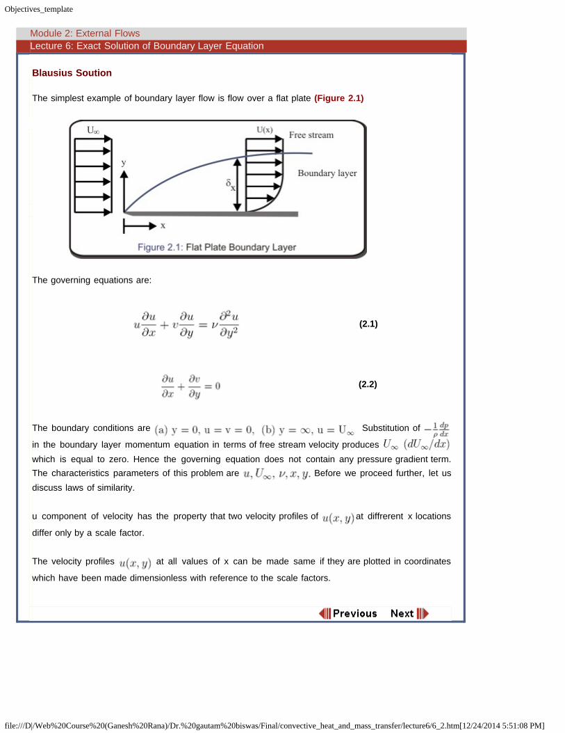
Blausius Soution
The simplest example of boundary layer flow is flow over a flat plate (Figure 2.1)
The governing equations are:
(2.1)
(2.2)
The boundary conditions are Substitution of
in the boundary layer momentum equation in terms of free stream velocity produces which is equal to zero. Hence the governing equation does not contain any pressure gradient term.The characteristics parameters of this problem are Before we proceed further, let usdiscuss laws of similarity.
u component of velocity has the property that two velocity profiles of at diffrerent x locations
differ only by a scale factor.
The velocity profiles at all values of x can be made same if they are plotted in coordinates
which have been made dimensionless with reference to the scale factors.

Objectives_template
file:///D|/Web%20Course%20(Ganesh%20Rana)/Dr.%20gautam%20biswas/Final/convective_heat_and_mass_transfer/lecture6/6_3.htm[12/24/2014 5:51:09 PM]
Module 2: External Flows Lecture 6: Exact Solution of Boundary Layer Equation
The local free stream velocity at is an obvious scale factor for u, because the dimensionless u
(x) varies with y between zero and unity at all sections. The scale factor for y, denoted by ,is
proportional to local boundary layer thickness so that y itself varies between zero and unity . Finally
(2.3)
Again, let us consider the statement of the problem :
(2.4)
Five variables involve two dimensions.Hence it is reducible for a dimensionless relation in terms of 3quantities .For boundary layer equations a special similarity variable is available and only two suchquantities are needed. When this is possible, the flow field is said to be self similar. For self similarflows the x-component of velocity has the property that two profiles of at different xlocations differ only by a scale factor that is at best a function of x.
(2.5)
For Blasuis problem the similarity law is :
(2.6)
Where
(2.7)
Or,
(2.8)
Or,
(2.9)

Objectives_template
file:///D|/Web%20Course%20(Ganesh%20Rana)/Dr.%20gautam%20biswas/Final/convective_heat_and_mass_transfer/lecture6/6_4.htm[12/24/2014 5:51:09 PM]
Module 2: External Flows Lecture 6: Exact Solution of Boundary Layer Equation
(2.10)
where if the stream function at the solid surface is set equal to 0.
(2.11)
(2.12)
Similarly ,
(2.13)
(2.14)
(2.15)
Substituting these terms in equation(2.1) and simplifying we get :
(2.16)

Objectives_template
file:///D|/Web%20Course%20(Ganesh%20Rana)/Dr.%20gautam%20biswas/Final/convective_heat_and_mass_transfer/lecture6/6_5.htm[12/24/2014 5:51:09 PM]
Module 2: External Flows Lecture 6: Exact Solution of Boundary Layer Equation
The boundary conditions are :
We know that at y = 0, u = 0 and v = 0. As a consequence, we can write
Similarly at results in
Equation (2.16) is a third order nonlinear differential equation. Blasius obtained this solution in theform of a series expanded around Let us assume a power series expansion of the (for smallvalues of )
(2.17)
Boundary conditions applied to above will produce
We derive another boundary condition from the physics of the problem: which leads to invoking this into above we get . Finally equation
(2.17) is substituted for into the Blasius equation, we find

Objectives_template
file:///D|/Web%20Course%20(Ganesh%20Rana)/Dr.%20gautam%20biswas/Final/convective_heat_and_mass_transfer/lecture6/6_6.htm[12/24/2014 5:51:09 PM]
Module 2: External Flows Lecture 6: Exact Solution of Boundary Layer Equation
Collecting diffrenet powers of and equating the corresponding coefficients equal to zero,we obtain
This will finally yield :
Now substituting the series for f ( )in terms of and :
(2.18)
or
Equation (2.18) satisfies boundary conditions at Applying boundary conditions at wehave
(21.9)
or ,The value of can be determined numerically to a good degree of accuracy.Howarth found

Objectives_template
file:///D|/Web%20Course%20(Ganesh%20Rana)/Dr.%20gautam%20biswas/Final/convective_heat_and_mass_transfer/lecture6/6_6.htm[12/24/2014 5:51:09 PM]

Objectives_template
file:///D|/Web%20Course%20(Ganesh%20Rana)/Dr.%20gautam%20biswas/Final/convective_heat_and_mass_transfer/lecture6/6_7.htm[12/24/2014 5:51:09 PM]
Module 2: External Flows Lecture 6: Exact Solution of Boundary Layer Equation
Numerical Approach :-Let us rewrite Equation (2.16)
as three first order differential equations in the following way:
(2.20)
(2.21)
(2.22)
The condition remains valid and
means
Note that the equations for f and G have initial values. The value for H(0) is not known. This is notan usual initial value problem We handle the problem as an initialvalue problem by choosing values ofH(0) and solving by numerical methods f ( );G ( ) and H ( ). In general G = 1 will not besatisfied for the function G arising from the numerical solution. We then choose other initial values ofH so that we find an H (0) which results in G = 1. This method is called SHOOTINGTECHNIQUE.
In Equations (2.20-2.22) the primes refer to dierentiation with respect to . The integration stepsfollowing a Runge-Kutta method are given below.
(2.23)
(2.24)
(2.25)

Objectives_template
file:///D|/Web%20Course%20(Ganesh%20Rana)/Dr.%20gautam%20biswas/Final/convective_heat_and_mass_transfer/lecture6/6_8.htm[12/24/2014 5:51:10 PM]
Module 2: External Flows Lecture 6: Exact Solution of Boundary Layer Equation
as one moves from The values of k;l and m are as follows :
(2.26)
(2.27)
(2.28)
In a similar way are calculated following standard formulae for Runge-Kuttaintegration.The functions Then at a distance from the wall, we have :
(2.29)
As it has been mentioned is unknown. H(0)=S must be determined such that the
condition is satisfied. The condition at innity is usually approximated at a nite valueof The value of H(0) now can be calculated by finding H (0) at which G crossesunity (Figure 2.2) Refer to figure (Figure 2.2) (b)

Objectives_template
file:///D|/Web%20Course%20(Ganesh%20Rana)/Dr.%20gautam%20biswas/Final/convective_heat_and_mass_transfer/lecture6/6_8.htm[12/24/2014 5:51:10 PM]

Objectives_template
file:///D|/Web%20Course%20(Ganesh%20Rana)/Dr.%20gautam%20biswas/Final/convective_heat_and_mass_transfer/lecture6/6_9.html[12/24/2014 5:51:10 PM]
Module 2: External Flows Lecture 6: Exact Solution of Boundary Layer Equation
Repeat the process by using H (0) and better of two initial values H(0).Thus the correct initialvalue will be determined.
Table 2.1
0 0 0 0.332060.2 0.00664 0.06641 0.331990.4 0.02656 0.13277 0.331470.8 0.10611 0.26471 0.327391.2 0.23795 0.39378 0.316591.6 0.42032 0.51676 0.296672.0 0.65003 0.62977 0.266752.4 0.92230 0.72899 0.228092.8 1.23099 0.81152 0.18401
0 0 0 0.332063.2 1.56911 0.87609 0.139133.6 1.92954 0.92333 0.09809
4.0 2.30576 0.95552 0.6424
4.4 2.69238 0.7587 0.038974.8 3.08534 0.98779 0.21875.0 3.28329 0.99155 0.015918.8 7.07923 1.00000 0.00000

Objectives_template
file:///D|/Web%20Course%20(Ganesh%20Rana)/Dr.%20gautam%20biswas/Final/convective_heat_and_mass_transfer/lecture6/6_10.htm[12/24/2014 5:51:10 PM]
Module 2: External Flows Lecture 6: Exact Solution of Boundary Layer Equation
Shear Stress
Each time examine versus for proper G . Compare the values with Schlichting. The
values are available in Table 2.1

Objectives_template
file:///D|/Web%20Course%20(Ganesh%20Rana)/Dr.%20gautam%20biswas/Final/convective_heat_and_mass_transfer/lecture6/6_10.htm[12/24/2014 5:51:10 PM]
Objectives_template
file:///D|/Web%20Course%20(Ganesh%20Rana)/Dr.%20gautam%20biswas/Final/convective_heat_and_mass_transfer/lecture6/6_11.htm[12/24/2014 5:51:10 PM]
Module 2: External Flows Lecture 6: Exact Solution of Boundary Layer Equation
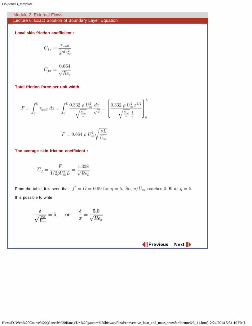
Local skin friction coefficient :
Total friction force per unit width
The average skin friction coefficient :
From the table, it is seen that
It is possible to write