The LIBOR market model - DHIS

The LIBOR market model

Responsible teacher: Anatoliy Malyarenko

August 30, 2004

AbstractContents of the lecture.

+ The LIBOR market model: theory.+ Context mapping+ Caps and floors.

– Typeset by FoilTEX –

MT1460 2005, period 3

The LIBOR market model

An interest rate derivative is a contract whosevalue depends on an underlying interest rate. Thevaluation of such a derivative may be dependent onthe value of the underlying rate at several differentfuture dates. Whilst models such as the Blackmodel assume log-normality for a single forwardrate or swap rate when pricing such derivatives as,caplets and swaptions respectively, many interestrate derivatives have future payoffs dependent onseveral underlying rates.

The LIBOR Market model also referred to, asthe “BGM/J model” is a multi-factor term structuremodel that allows for future volatility patterns tobe considered. The LIBOR Market frameworkuses LIBOR rates for modeling, which are marketobservable and has therefore become very popularamong traders. Existing interest rate models arelimited by the fact that, first, they model non-marketobservable quantities and, secondly, often use onefactor.

– Typeset by FoilTEX – 1

MT1460 2005, period 3

Black model

The standard model for valuing interest rateoptions, caps/floors and European swaptions, is theBlack model. The Black model is used by traders inthe market to price these derivatives and as will beseen later on, the analytical Black formulas will playa key role when calibrating the LIBOR Market model.

Before attempting to calculate values (prices) forthese interest rate derivatives it is necessary to makecertain assumptions about the underlying rates.

The basic assumptions under the Black modelare:

+ the underlying forward rate or swap rate is a lognormally distributed random variable;

+ the volatility of the underlying is constant;

+ prices are arbitrage free;

+ there is continuous trading in all instruments.


MT1460 2005, period 3

Forward rates

Before defining the underlying variables, therates, it is important to introduce the concept ofdiscount bonds. Discount bonds are traded in themarket but more commonly are so called coupon-bearing bonds. These have several guaranteedfuture cash flows instead of just one. The coupon-bearing bonds can be reduced to a set of ordinarydiscount bonds. In fact, to get the price of a discountbond one often imputes this price from (suitable)coupon-bearing bonds.

A contract, which gives the holder an amount 1at some future date T , is referred to as discountbond. 1 is called the notional or face value and Tis referred to as the maturity date. The price at timet of a discount bond with maturity T and face value 1is denoted by P(t,T ).

To deal with this assumption of a continuumof prices (also known as the discount function),in practice one selects a set of discount bondprices (the benchmark instruments) and then simplyinterpolates between them. For theoretical purposes


MT1460 2005, period 3

it is (almost) always assumed that there is a discountbond available for every maturity date T .

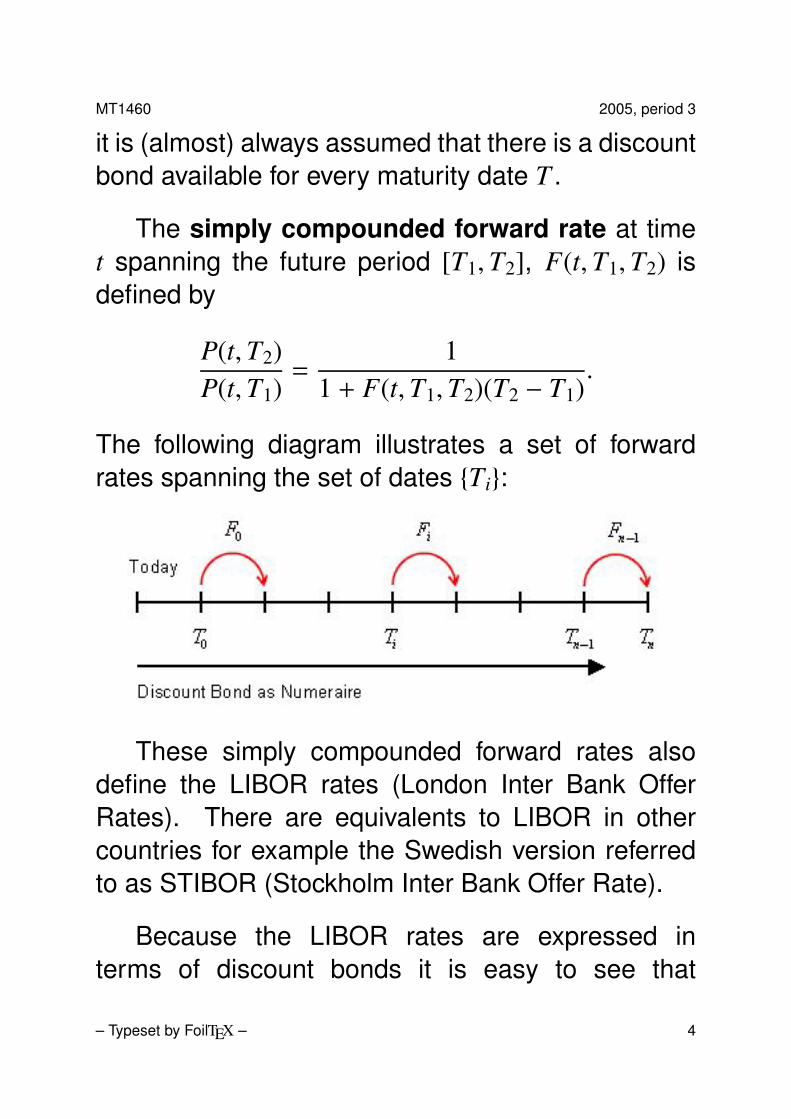
The simply compounded forward rate at timet spanning the future period [T1,T2], F(t,T1,T2) isdefined by

P(t,T2)P(t,T1)

=1

1 + F(t,T1,T2)(T2 − T1).

The following diagram illustrates a set of forwardrates spanning the set of dates {Ti}:

These simply compounded forward rates alsodefine the LIBOR rates (London Inter Bank OfferRates). There are equivalents to LIBOR in othercountries for example the Swedish version referredto as STIBOR (Stockholm Inter Bank Offer Rate).

Because the LIBOR rates are expressed interms of discount bonds it is easy to see that


MT1460 2005, period 3

these could be an alternative to the discountbonds when building the discount function in certaincircumstances. More explicitly, where one wasreceiving money at a discrete set of known futuredates T1, . . . , Tn, and wanted to calculate todaysvalue of these future cash flows, then it would besufficient to know the value of the discount functionat these dates given by a discrete set of LIBOR rates.


MT1460 2005, period 3

Caps and floors

A caplet connected with the forward rateF(Ti,Ti,Ti + τi) and with strike k, is a contract, whichat time Ti + τi gives the holder the cash flow:

τi max{F(Ti,Ti,Ti + τi) − k, 0}.

A cap is a set of caplets. The price of a caplet usingthe Black model is given by:

Vi(0) = P(0,Ti+1)Niτi(Fi(0)Φ(a1i) − kΦ(a2i)),

where

k the strike of an interest rate capVi value of ith capletτi time to maturity of the ith capletTi reset dates of forward rateP discount factorNi notional principal of each capletF forward rateτi tenor or Ti+1 − Ti.


MT1460 2005, period 3

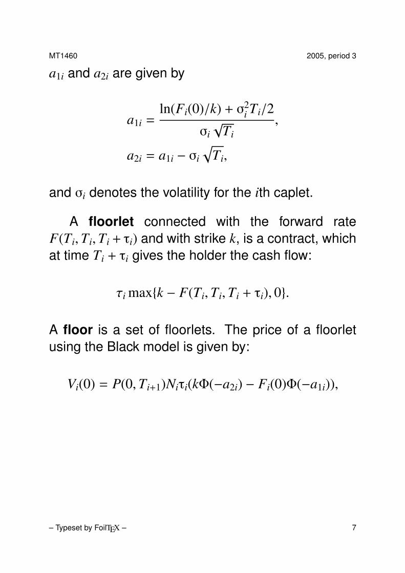
a1i and a2i are given by

a1i =ln(Fi(0)/k) + σ2

i Ti/2

σi√

Ti,

a2i = a1i − σi

√Ti,

and σi denotes the volatility for the ith caplet.

A floorlet connected with the forward rateF(Ti,Ti,Ti + τi) and with strike k, is a contract, whichat time Ti + τi gives the holder the cash flow:

τi max{k − F(Ti,Ti,Ti + τi), 0}.

A floor is a set of floorlets. The price of a floorletusing the Black model is given by:

Vi(0) = P(0,Ti+1)Niτi(kΦ(−a2i) − Fi(0)Φ(−a1i)),


MT1460 2005, period 3

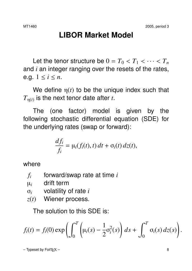
LIBOR Market Model

Let the tenor structure be 0 = T0 < T1 < · · · < Tn

and i an integer ranging over the resets of the rates,e.g. 1 ≤ i ≤ n.

We define η(t) to be the unique index such thatTη(t) is the next tenor date after t.

The (one factor) model is given by thefollowing stochastic differential equation (SDE) forthe underlying rates (swap or forward):

d fifi= µi( fi(t), t) dt + σi(t) dz(t),

where

fi forward/swap rate at time iµi drift termσi volatility of rate iz(t) Wiener process.

The solution to this SDE is:

fi(t) = fi(0) exp(∫ T

0

(µi(s) −

12σ

2i (s)

)ds +

∫ T

0σi(s) dz(s)

).


MT1460 2005, period 3

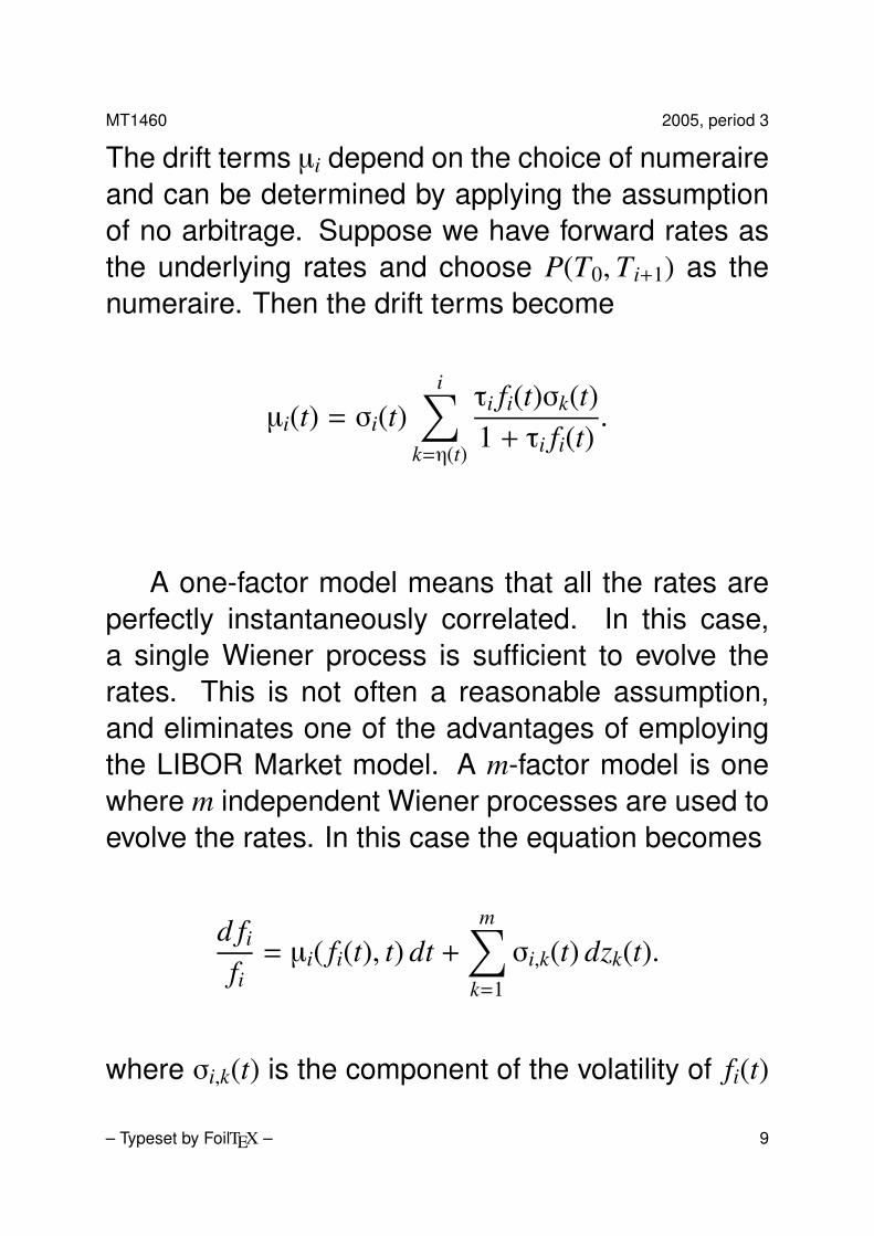
The drift terms µi depend on the choice of numeraireand can be determined by applying the assumptionof no arbitrage. Suppose we have forward rates asthe underlying rates and choose P(T0,Ti+1) as thenumeraire. Then the drift terms become

µi(t) = σi(t)i∑

k=η(t)

τi fi(t)σk(t)1 + τi fi(t)

.

A one-factor model means that all the rates areperfectly instantaneously correlated. In this case,a single Wiener process is sufficient to evolve therates. This is not often a reasonable assumption,and eliminates one of the advantages of employingthe LIBOR Market model. A m-factor model is onewhere m independent Wiener processes are used toevolve the rates. In this case the equation becomes

d fifi= µi( fi(t), t) dt +

m∑k=1

σi,k(t) dzk(t).

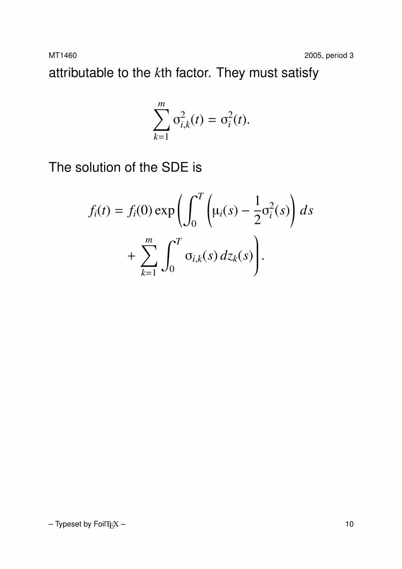
where σi,k(t) is the component of the volatility of fi(t)


MT1460 2005, period 3

attributable to the kth factor. They must satisfy

m∑k=1

σ2i,k(t) = σ

2i (t).

The solution of the SDE is

fi(t) = fi(0) exp(∫ T

0

(µi(s) −

12σ

2i (s)

)ds

+

m∑k=1

∫ T

0σi,k(s) dzk(s)

.


MT1460 2005, period 3

Cap volatility calibration

Assume that each underlying rate fi(t) has alognormal distribution with variance equal to σ2

Bt,where σ2

B is the implied Black volatility, which canbe read from the market. Then the instantaneousvolatility at reset for each rate is related to the aboveexpression in the following way:

∫ Ti

0σ

2i (t) dt = σ2

BTi. (1)

There are (infinitely) many solutions to theseequations, and our goal is to pick one that fits ourneeds. Let

σ(t) = (a + bt)e−ct + d

andσi(t) = kiσ(Ti − t).

The calibration proceeds as follows.

À Find values on the constants a, b, c, and d suchthat equation (1) fit as close as possible.


MT1460 2005, period 3

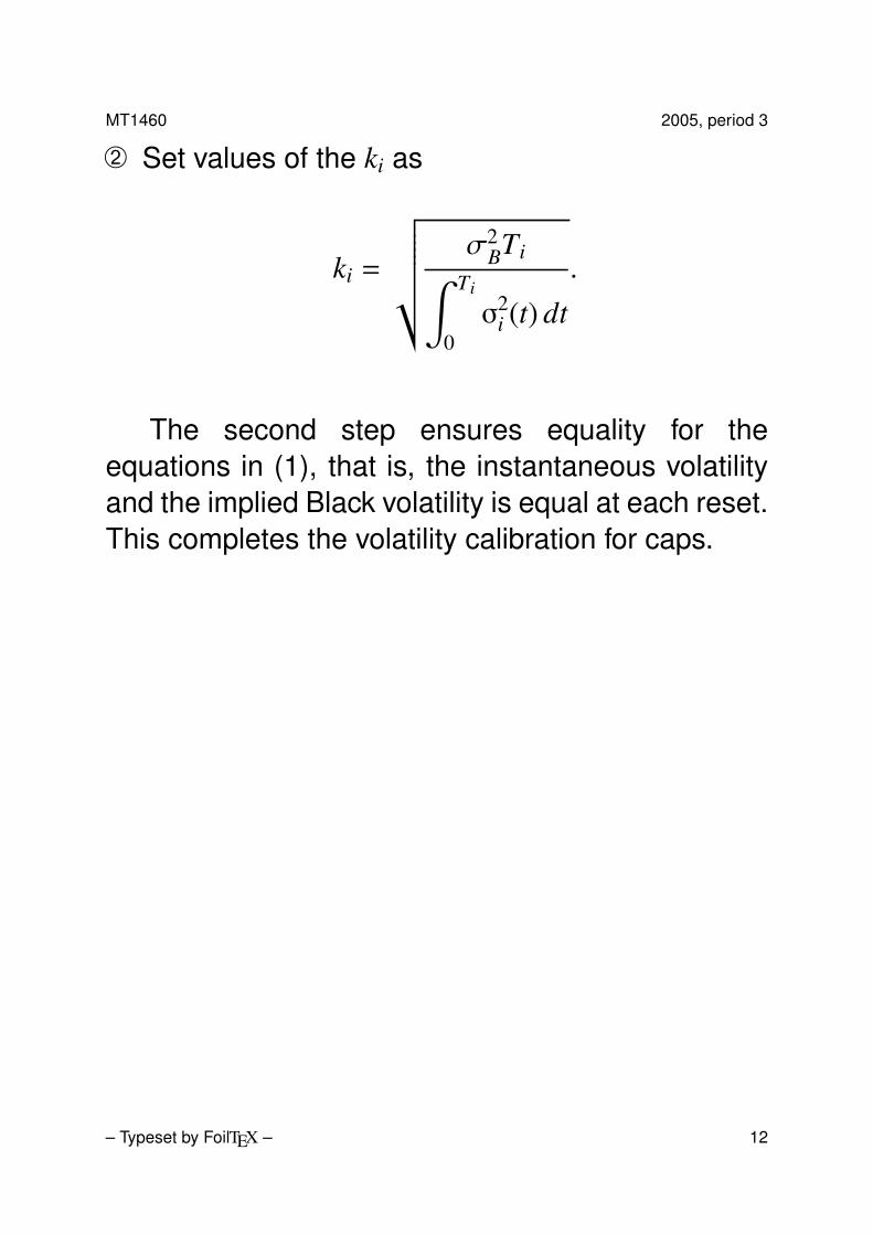
Á Set values of the ki as

ki =

√√√√√√√ σ2BTi∫ Ti

0σ

2i (t) dt

.

The second step ensures equality for theequations in (1), that is, the instantaneous volatilityand the implied Black volatility is equal at each reset.This completes the volatility calibration for caps.


MT1460 2005, period 3

Context mapping

In order to use the LIBOR Market Model whenvaluing instruments the following context mappingsmust be performed:

À Map the instrument to the Core ValuationFunction > LIBOR Market Model. This mappingtells FRONT ARENA to value the instrument withthe LIBOR Market Model.

Á Map the instrument to an appropriate correlationmatrix. The LIBOR Market Model requires acorrelation matrix as input, and this mappingmakes sure it gets one.

Â Map the instrument to an appropriate volatilityLandscape. If the instrument is a Cap/Floorit suffices to map a volatility Landscape to therate index. If the instrument is a Swaption, wemust, in addition, map a volatility Landscape tothe instrument itself. The LIBOR Market Modelthen uses these volatilities (or this volatility if theinstrument is a Cap/Floor) in its calibration step.


MT1460 2005, period 3

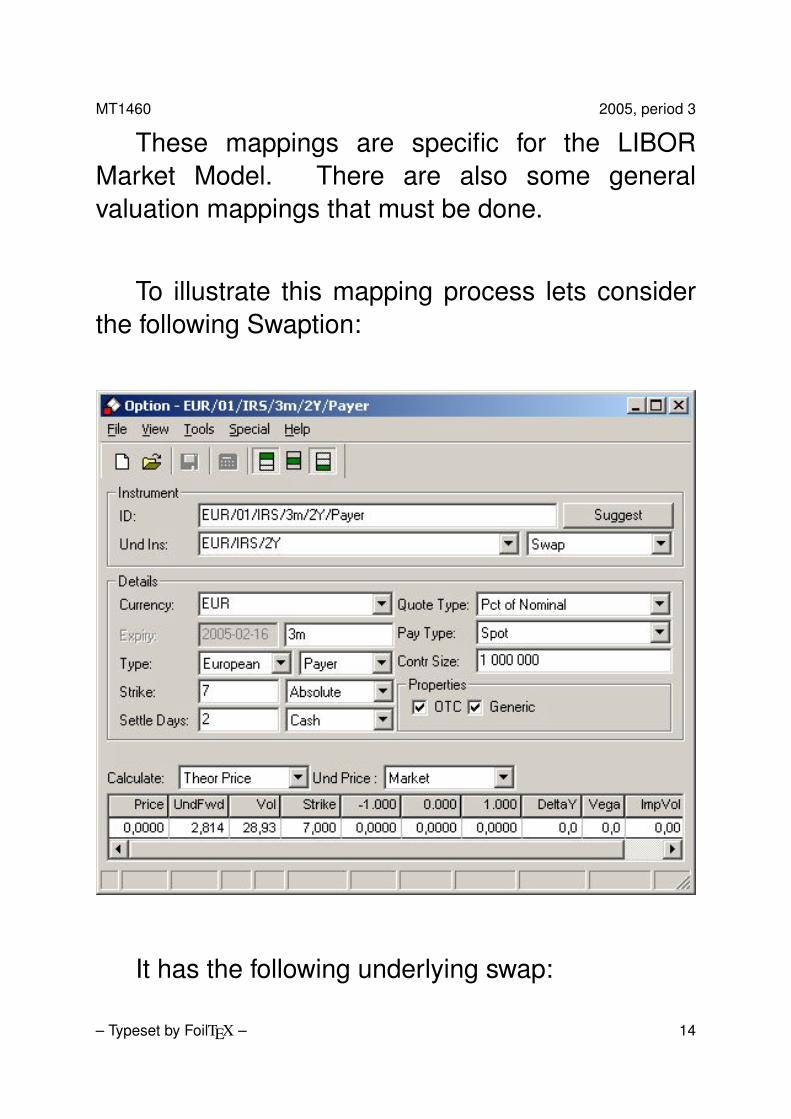
These mappings are specific for the LIBORMarket Model. There are also some generalvaluation mappings that must be done.

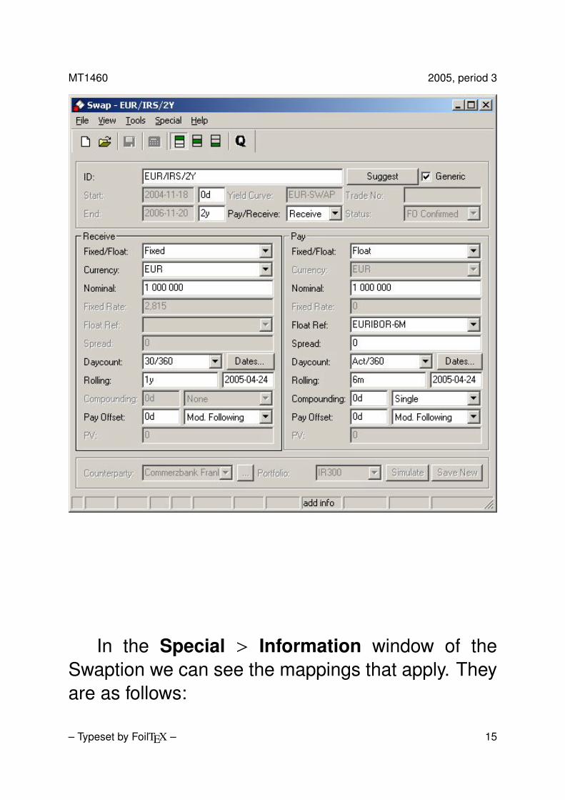
To illustrate this mapping process lets considerthe following Swaption:

It has the following underlying swap:


MT1460 2005, period 3

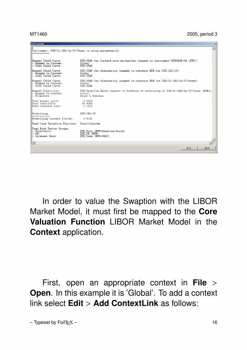
In the Special > Information window of theSwaption we can see the mappings that apply. Theyare as follows:


MT1460 2005, period 3

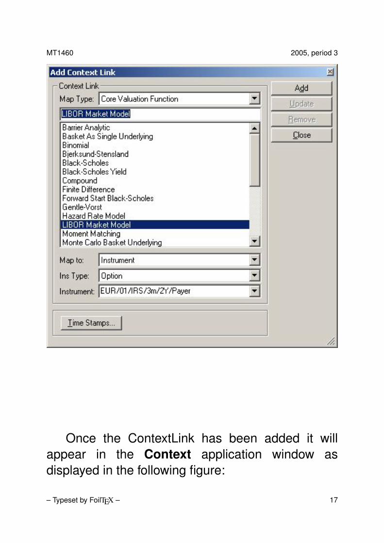
In order to value the Swaption with the LIBORMarket Model, it must first be mapped to the CoreValuation Function LIBOR Market Model in theContext application.

First, open an appropriate context in File >Open. In this example it is ’Global’. To add a contextlink select Edit > Add ContextLink as follows:


MT1460 2005, period 3

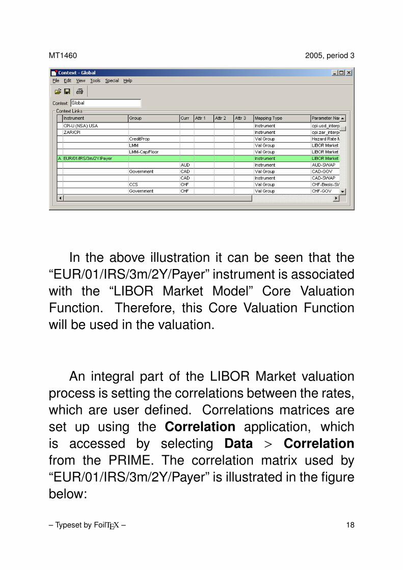
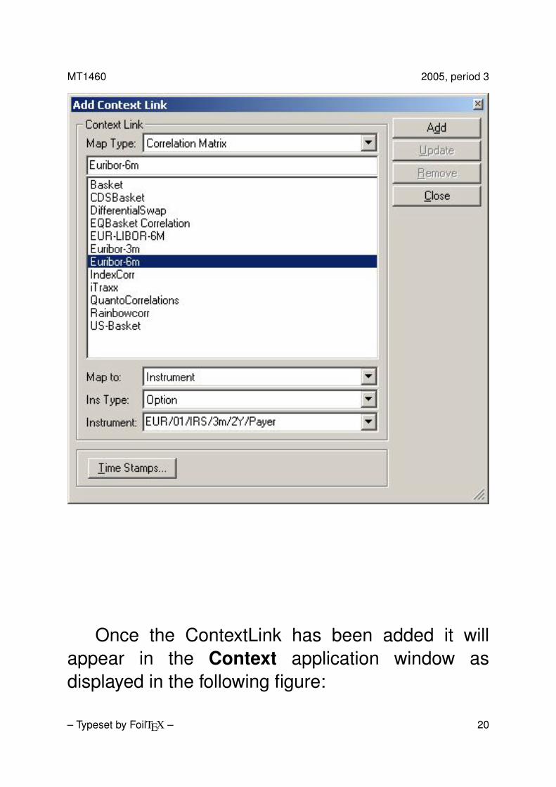
Once the ContextLink has been added it willappear in the Context application window asdisplayed in the following figure:


MT1460 2005, period 3

In the above illustration it can be seen that the“EUR/01/IRS/3m/2Y/Payer” instrument is associatedwith the “LIBOR Market Model” Core ValuationFunction. Therefore, this Core Valuation Functionwill be used in the valuation.

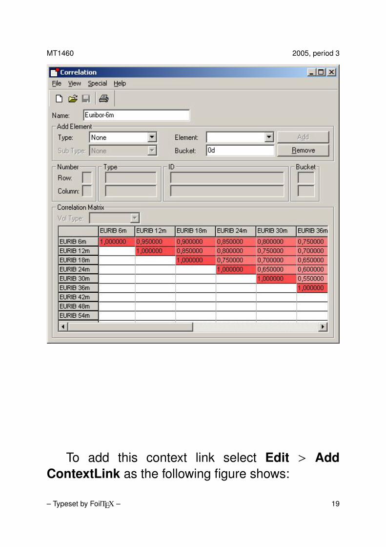
An integral part of the LIBOR Market valuationprocess is setting the correlations between the rates,which are user defined. Correlations matrices areset up using the Correlation application, whichis accessed by selecting Data > Correlationfrom the PRIME. The correlation matrix used by“EUR/01/IRS/3m/2Y/Payer” is illustrated in the figurebelow:


MT1460 2005, period 3

To add this context link select Edit > AddContextLink as the following figure shows:


MT1460 2005, period 3

Once the ContextLink has been added it willappear in the Context application window asdisplayed in the following figure:


MT1460 2005, period 3

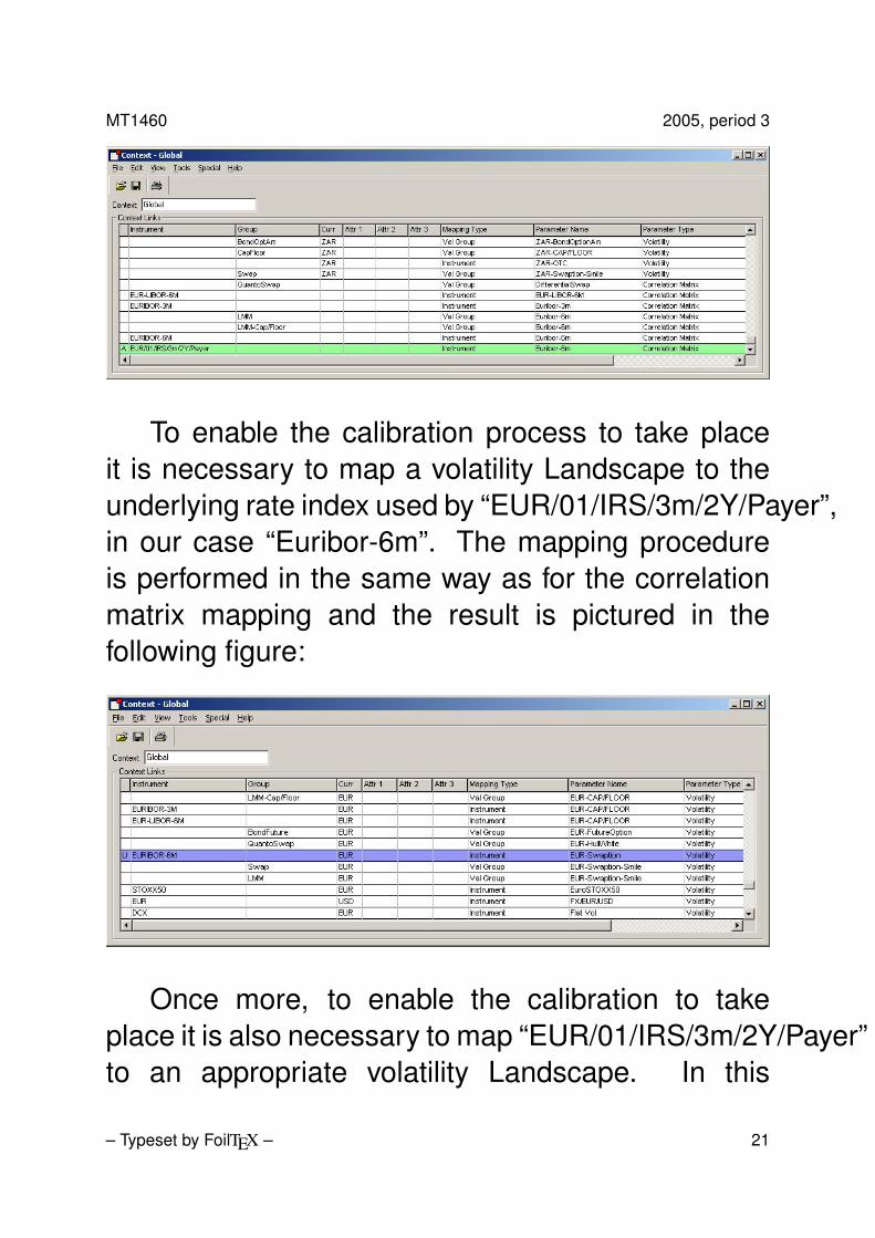
To enable the calibration process to take placeit is necessary to map a volatility Landscape to theunderlying rate index used by “EUR/01/IRS/3m/2Y/Payer”,in our case “Euribor-6m”. The mapping procedureis performed in the same way as for the correlationmatrix mapping and the result is pictured in thefollowing figure:

Once more, to enable the calibration to takeplace it is also necessary to map “EUR/01/IRS/3m/2Y/Payer”to an appropriate volatility Landscape. In this


MT1460 2005, period 3

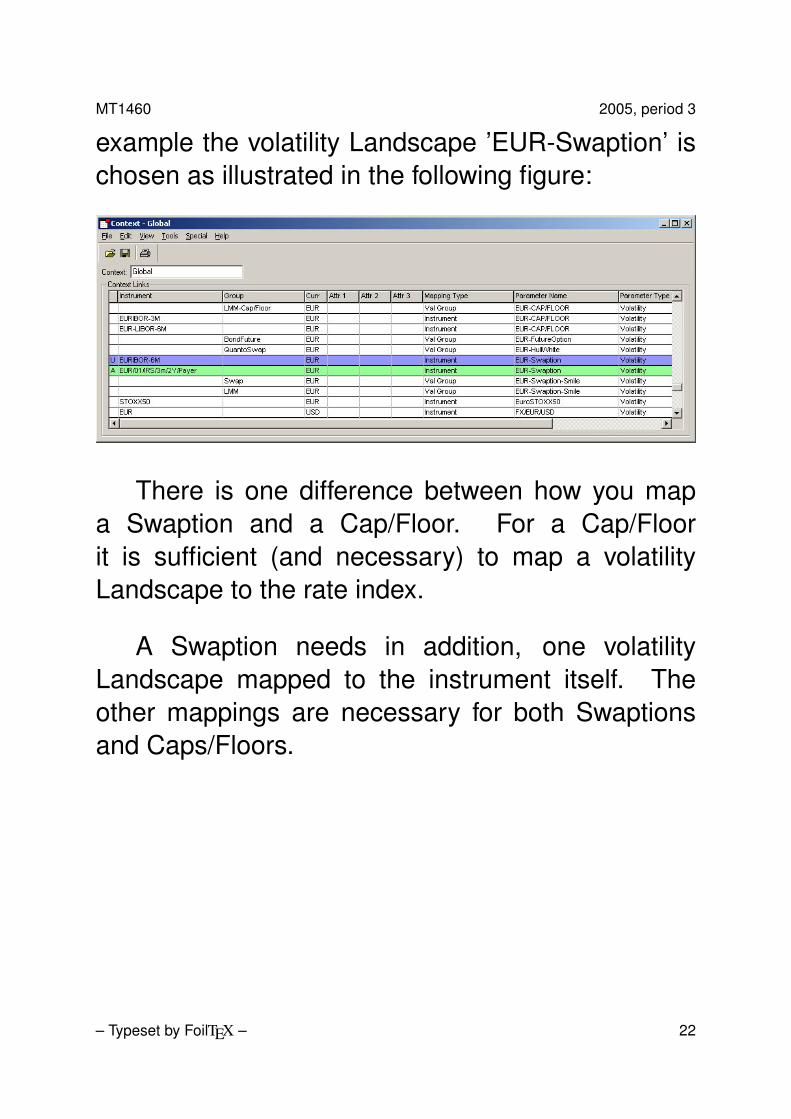
example the volatility Landscape ’EUR-Swaption’ ischosen as illustrated in the following figure:

There is one difference between how you mapa Swaption and a Cap/Floor. For a Cap/Floorit is sufficient (and necessary) to map a volatilityLandscape to the rate index.

A Swaption needs in addition, one volatilityLandscape mapped to the instrument itself. Theother mappings are necessary for both Swaptionsand Caps/Floors.


MT1460 2005, period 3

Valuation parameters

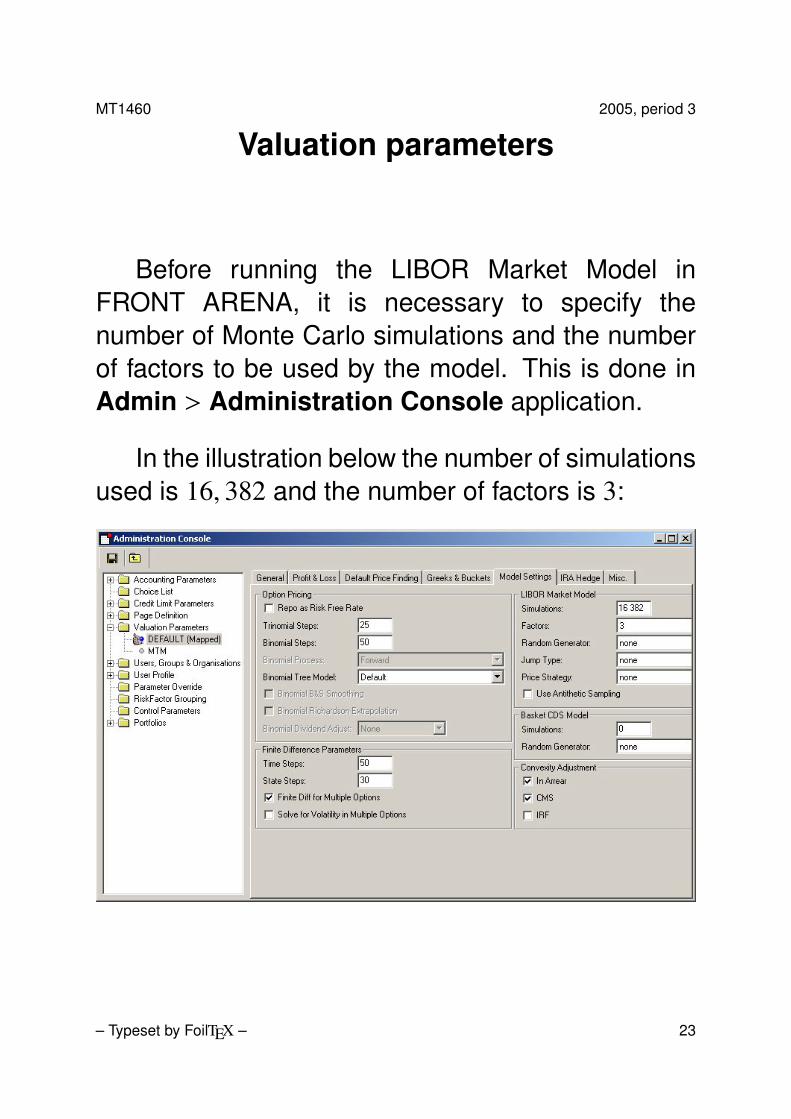
Before running the LIBOR Market Model inFRONT ARENA, it is necessary to specify thenumber of Monte Carlo simulations and the numberof factors to be used by the model. This is done inAdmin > Administration Console application.

In the illustration below the number of simulationsused is 16, 382 and the number of factors is 3:


MT1460 2005, period 3

Caps and floors

It is assumed that all the necessary settings, asdiscussed before, have been taken care of. Thedifferent Caps/Floors that can be valued in FRONTARENA using the LIBOR Market Model are plainvanilla, “Ratchet”, “Sticky”, “Momentum”, “Flexi”, and“Chooser”.

All are described there, with the exception of aplain vanilla. Assuming that the correct settings havebeen done, entering a plain vanilla Cap/Floor andvalue it with the LIBOR Market Model is no differenthad it been valued with Black’s Model.

From hereon we only discuss Caps. Definitionsof the Floors can easily be derived from thecorresponding Cap definitions.


MT1460 2005, period 3

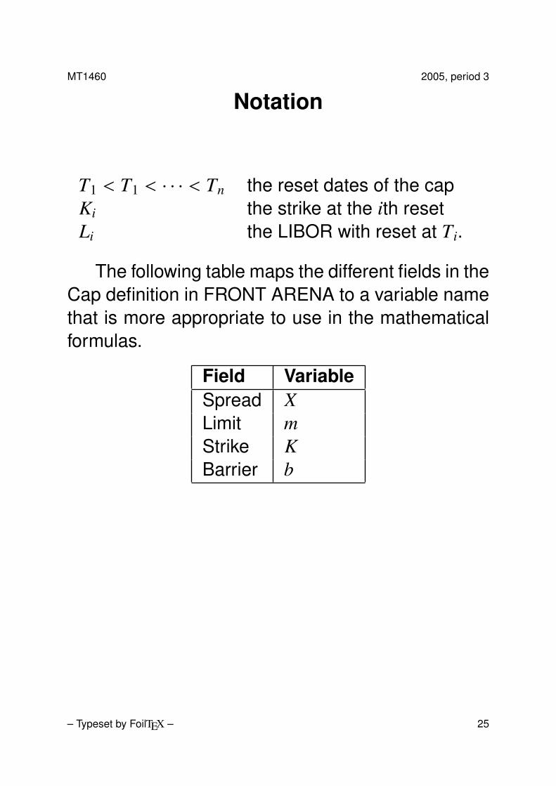
Notation

T1 < T1 < · · · < Tn the reset dates of the capKi the strike at the ith resetLi the LIBOR with reset at Ti.

The following table maps the different fields in theCap definition in FRONT ARENA to a variable namethat is more appropriate to use in the mathematicalformulas.

Field VariableSpread XLimit mStrike KBarrier b


MT1460 2005, period 3

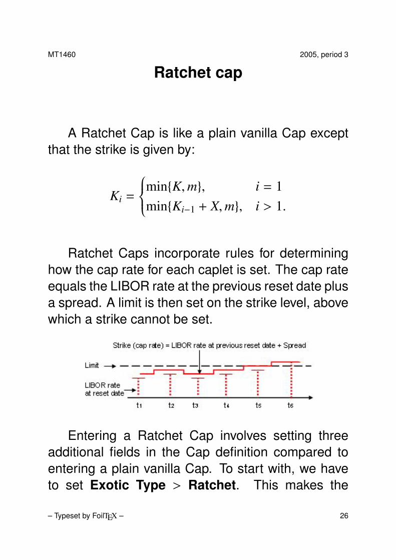
Ratchet cap

A Ratchet Cap is like a plain vanilla Cap exceptthat the strike is given by:

Ki =

min{K,m}, i = 1min{Ki−1 + X,m}, i > 1.

Ratchet Caps incorporate rules for determininghow the cap rate for each caplet is set. The cap rateequals the LIBOR rate at the previous reset date plusa spread. A limit is then set on the strike level, abovewhich a strike cannot be set.

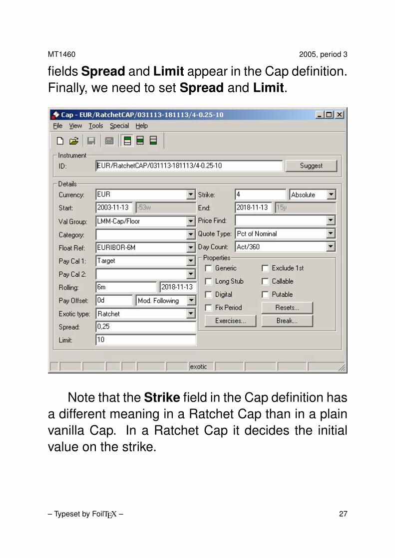
Entering a Ratchet Cap involves setting threeadditional fields in the Cap definition compared toentering a plain vanilla Cap. To start with, we haveto set Exotic Type > Ratchet. This makes the


MT1460 2005, period 3

fields Spread and Limit appear in the Cap definition.Finally, we need to set Spread and Limit.

Note that the Strike field in the Cap definition hasa different meaning in a Ratchet Cap than in a plainvanilla Cap. In a Ratchet Cap it decides the initialvalue on the strike.


MT1460 2005, period 3

Sticky cap

A Sticky Cap is like a plain vanilla Cap except thatthe strike is given by:

Ki =

min{K,m}, i = 1min{min{Ki−1, Li−1} + X,m}, i > 1.

In a Sticky Cap, the cap rate equals the previouscapped rate plus a spread. A limit is then set on thestrike level, above which a strike cannot be set.

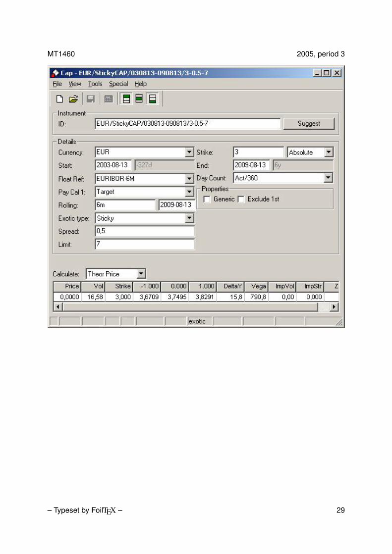
Entering a Sticky Cap involves setting threeadditional fields in the Cap definition compared toentering a plain vanilla Cap. To start with, it isnecessary to set Exotic Type > Sticky. This makesthe fields Spread and Limit appear in the Capdefinition. Finally, we need to set Spread and Limit.

Note that the Strike field in the Cap definition hasa different meaning in a ’Sticky’ Cap than in a plainvanilla Cap. In a ’Sticky’ Cap it decides the initialvalue on the strike.


MT1460 2005, period 3


MT1460 2005, period 3

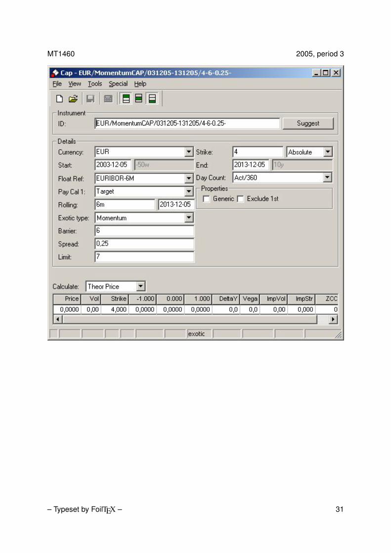
Momentum cap

A Momentum Cap is like a plain vanilla Capexcept that the strike is given by:

Ki =

min{K,m}, i = 1min{Ki−1 + X,m}, i > 1, Li − b > Li−1

min{Ki−1,m}, i > 1, Li − b ≤ Li−1.

Entering a Momentum Cap involves setting fouradditional fields in the Cap definition compared toentering a plain vanilla Cap. To start with, we haveto set Exotic Type > Momentum. This makes thefields Barrier, Spread and Limit appear in the Capdefinition. Finally, we need to set Barrier, Spreadand Limit.

Note that the Strike field in the Cap definition hasa different meaning in a Momentum Cap than in aplain vanilla Cap. In a Momentum Cap it decides theinitial value on the strike.


MT1460 2005, period 3


MT1460 2005, period 3

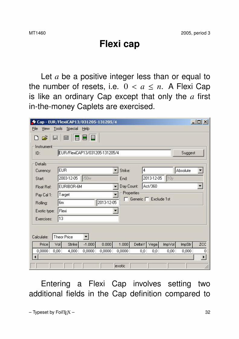
Flexi cap

Let a be a positive integer less than or equal tothe number of resets, i.e. 0 < a ≤ n. A Flexi Capis like an ordinary Cap except that only the a firstin-the-money Caplets are exercised.

Entering a Flexi Cap involves setting twoadditional fields in the Cap definition compared to


MT1460 2005, period 3

entering a plain vanilla Cap. To start with, wehave to set Exotic Type > Flexi. This makes thefield Exercises appear in the Cap definition, whichcorresponds to the integer a seen above. Finally, weneed to set this field.


MT1460 2005, period 3

Chooser cap

Let a be a positive integer less than or equal tothe number of resets, i.e. 0 < a ≤ n. A chooserCap is like a Flexi Cap except that the contract holdercan choose which a Caplets to exercise. Once thereset of a Caplet has taken place, it can no longerbe chosen.

This is how the LIBOR Market Model in FRONTARENA values a chooser Cap. Of course, it includesall the chosen Caplets. Suppose that c Caplets havebeen chosen, and that c < a ≤ n. This means thatthere are still a − c Caplets that can be chosen. Inthis case it picks a − c, or as many as possible butno more than a − c, of the remaining Caplets withhighest present value. In other words, it employs anoptimal strategy for the remaining of the Cap.

Initially, entering a chooser Cap involves settingtwo additional fields in the Cap definition comparedto entering a plain vanilla Cap. To start with, we haveto set Exotic Type > Chooser. This makes thefield Exercises appear in the Cap definition, whichcorresponds to the integer a seen above. Finally, we


MT1460 2005, period 3

need to set this field.

During the life of the chooser Cap we mustchoose which of the a Caplets to exercise. Wechoose a Caplet by entering a non-zero value in therecord fixed time of the database table CashFlow.

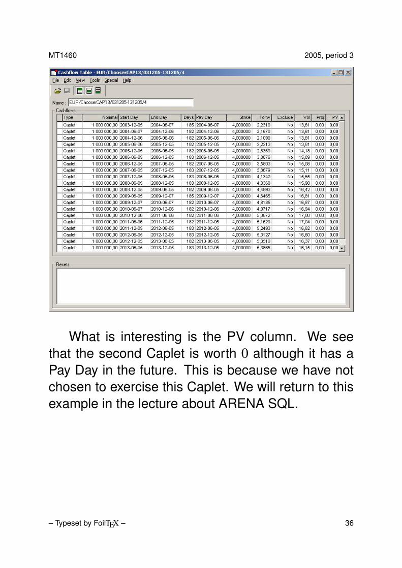
Now we have defined the chooser Cap. Let ustake a look at the Tools > Cash Flow Table whenwe have not chosen any Caplet to exercise.


MT1460 2005, period 3

What is interesting is the PV column. We seethat the second Caplet is worth 0 although it has aPay Day in the future. This is because we have notchosen to exercise this Caplet. We will return to thisexample in the lecture about ARENA SQL.


MT1460 2005, period 3

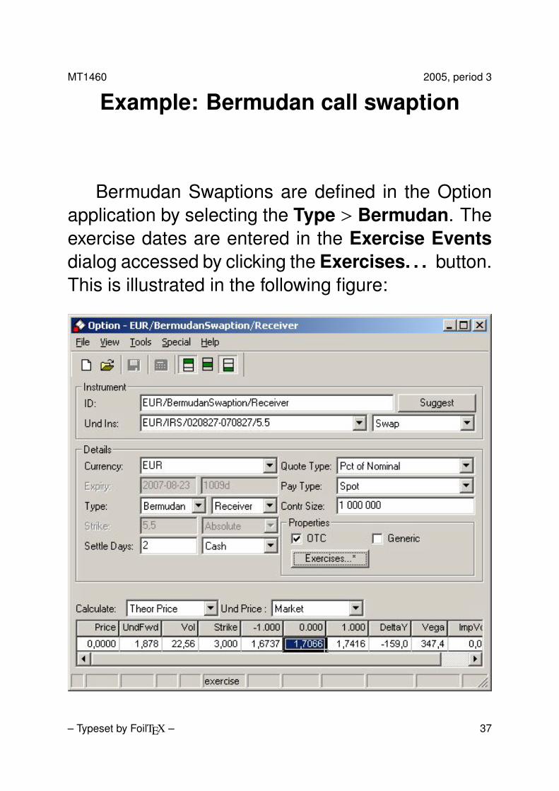
Example: Bermudan call swaption

Bermudan Swaptions are defined in the Optionapplication by selecting the Type > Bermudan. Theexercise dates are entered in the Exercise Eventsdialog accessed by clicking the Exercises. . . button.This is illustrated in the following figure:


MT1460 2005, period 3

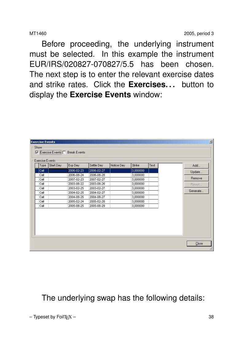
Before proceeding, the underlying instrumentmust be selected. In this example the instrumentEUR/IRS/020827-070827/5.5 has been chosen.The next step is to enter the relevant exercise datesand strike rates. Click the Exercises. . . button todisplay the Exercise Events window:

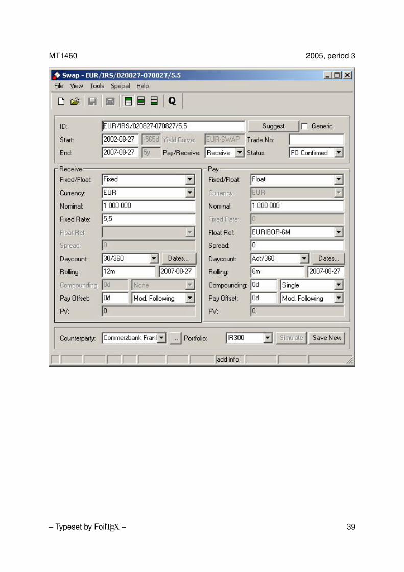
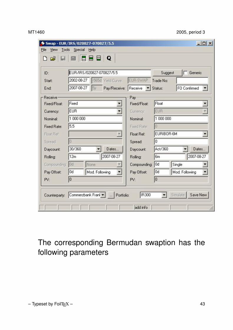
The underlying swap has the following details:


MT1460 2005, period 3


MT1460 2005, period 3

Exercises

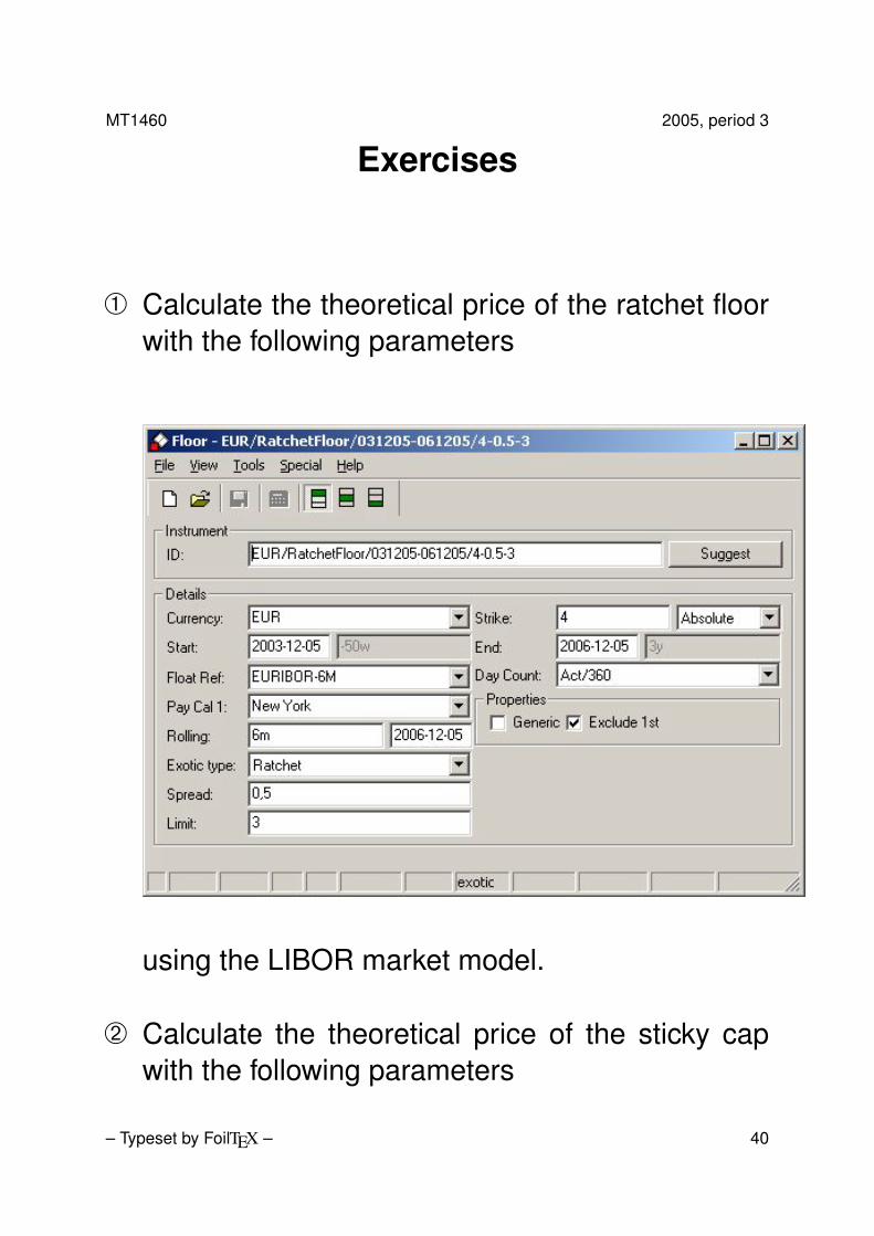
À Calculate the theoretical price of the ratchet floorwith the following parameters

using the LIBOR market model.

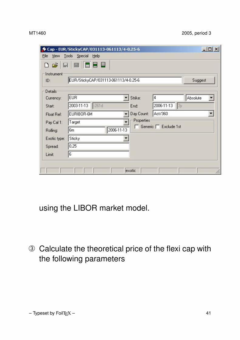
Á Calculate the theoretical price of the sticky capwith the following parameters


MT1460 2005, period 3


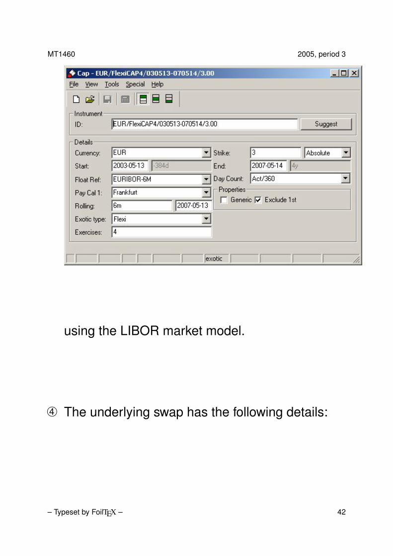
Â Calculate the theoretical price of the flexi cap withthe following parameters


MT1460 2005, period 3


Ã The underlying swap has the following details:


MT1460 2005, period 3

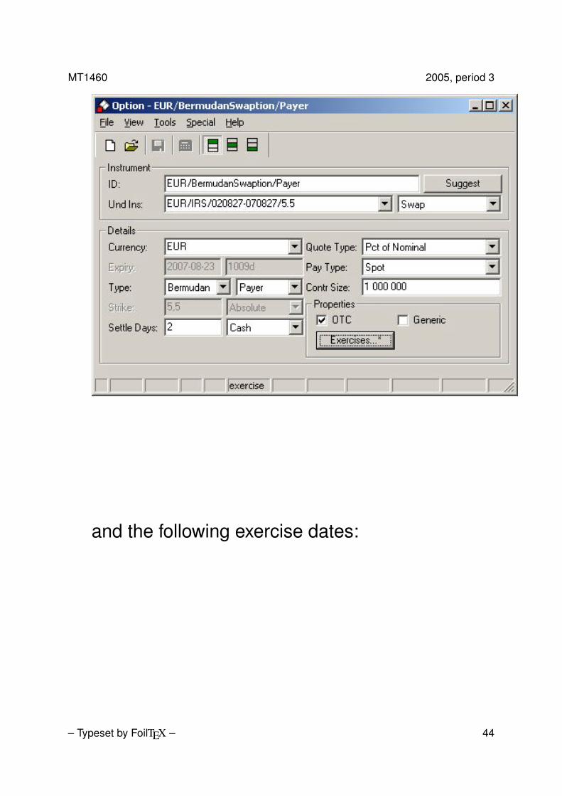
The corresponding Bermudan swaption has thefollowing parameters


MT1460 2005, period 3

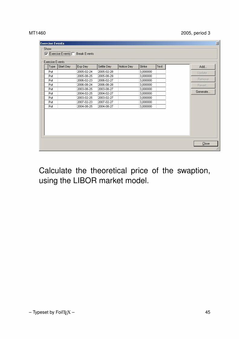
and the following exercise dates:


MT1460 2005, period 3

Calculate the theoretical price of the swaption,using the LIBOR market model.


Documents

The LIBOR market model - DHIS