Embed Size (px)
Citation preview
Ann Inst Stat Math (2015) 67:39–73DOI 10.1007/s10463-013-0438-5
The limited information maximum likelihood approachto dynamic panel structural equation models
Kentaro Akashi · Naoto Kunitomo
Received: 28 January 2013 / Revised: 15 October 2013 / Published online: 13 December 2013© The Institute of Statistical Mathematics, Tokyo 2013
Abstract We develop the panel-limited information maximum likelihood approachfor estimating dynamic panel structural equation models. When there are dynamiceffects and endogenous variables with individual effects at the same time, the LIMLmethod for the filtered data does give not only a consistent estimator and asymp-totic normality, but also attains the asymptotic bound when the number of orthogonalconditions is large. Our formulation includes Alvarez and Arellano (Econometrica71:1121–1159, 2003), Blundell and Bond (Econ Rev 19-3:321–340, 2000) and otherlinear dynamic panel models as special cases.
Keywords Dynamic panel structural equation · LIML · Many orthogonalconditions · Forward and backward filters · Optimality
1 Introduction
There have been a number of panel data available and their analyses have been grow-ing in many applied fields of economics in the past decades. Statistical methods on
Electronic supplementary material The online version of this article (doi:10.1007/s10463-013-0438-5)contains supplementary material, which is available to authorized users.
K. AkashiFaculty of Economics, Gakushuin University,Toshima-ku, Mejiro 1-5-1, Tokyo 113-0033, Japane-mail: [email protected]
N. Kunitomo (B)Graduate School of Economics, University of Tokyo,Bunkyo-ku, Hongo 7-3-1, Tokyo 113-0033, Japane-mail: [email protected]
123
40 K. Akashi, N. Kunitomo
panel data have been developed, which are indispensable in econometrics (see Hsiao2003, Arellano 2003 and Baltagi 2005 for instance). The dynamic panel models havebeen often used in empirical applications and the earlier investigations were fromAnderson and Hsiao (1981, 1982). In a pioneering work Alvarez and Arellano (2003)investigated the asymptotic behavior of alternative estimation methods in a dynamicpanel regression model when both N (the number of individuals) and T (the numberof observation periods) are large. Our approach is related to these studies.
There are still non-trivial statistical problems on estimating dynamic panel econo-metric models to be investigated. In particular, when there are lagged endogenousvariables with individual effects and the simultaneity effects in the structural equationof interest exist at the same time, the standard econometric methods including theGMM (generalized method of moments) in the econometric literature or the estimat-ing equation (EE) method in the statistics literature do not necessarily work well due tothe presence of individual effects, which cause the problem of incidental parameterswhen we have a long time-horizon.
In this paper, we propose the panel-limited information maximum likelihood(PLIML) approach to dynamic panel structural equation models. It is a simple exten-sion of the limited information maximum likelihood (LIML) method, which was orig-inally developed by Anderson and Rubin (1949, 1950). We intend to apply the LIMLmethod to the dynamic panel structural models when there are dynamic effects andendogenous variables with individual effects at the same time. We need to modifythe LIML method to handle the dynamic panel models with individual effects andpossibly many orthogonal conditions because the individual effects in panel structuralequations cause a source of endogeneity between the explanatory (or instrumental)variables and the explained variables, and we propose to use the filtering procedures.The PLIML method gives a consistent estimator and attains the asymptotic efficiencybound for general dynamic panel structural equation models when the relative ratioT/N is not small. In macro-panel data or long panel data, T (the number of observa-tions over time) can be substantial and it is often important to estimate the dynamiceffects in the structural equation of interest. When the panel dimensions (N , T ) andthe number of available instruments are not small, the approximations of the limitingdistributions of estimators and test statistics based on the standard asymptotics areoften poor and we need another asymptotic theory, which corresponds to the large-K2asymptotics developed by Kunitomo (1980) as an early study and it has been recentlyre-examined by Anderson et al. (2005, 2010, 2011).
In our framework of study, we shall consider alternative ways of filtering procedurefor the original data before estimation systematically, namely, the forward-filteringand the backward-filtering. We shall show that the LIML estimation has an advanta-geous aspect when we use the forward-filtering and utilize many orthogonal conditionsin particular. Also the usage of the backward-filtering for instruments can decreasethe effects of a large number of possible instruments and the doubly-filtered LIMLbecomes asymptotically less biased. In a companion paper, Akashi and Kunitomo(2012) further have investigated the details of the finite sample properties of alterna-tive estimation methods such as the WG (within groups), the GMM and the PLIMLestimators in a simple setting when there are two equations. The formulation of thispaper is much more general and we shall show that their findings and results on the
123
The LIML approach to dynamic panel SEMs 41
finite sample and asymptotic properties of alternative estimators are relevant for moregeneral dynamic panel structural equations. A related work to the LIML method inpanel econometric analysis would be Alonso-Borrego and Arellano (1999).
In Sect. 2, we state the formulation of models and define the alternative estimationmethods of unknown parameters in the dynamic panel structural equation model withpossibly many instruments and the filtering procedures. Then in Sect. 3, we give theresults on the asymptotic properties of the LIML and GMM estimation methods andthe result on the asymptotic optimality. In Sect. 4, we shall report on the finite sampleproperties based on a set of Monte Carlo simulations. Then in Sect. 5, some concludingremarks will be given. The proofs of our theorems will be given in Sect. 6.
2 LIML approach to dynamic panel structural equation
2.1 Model
We consider the estimation problem of a dynamic panel structural equation with indi-vidual effects in the form
y(1)i t = β′2 y(2)i t + γ
′1z(1)i t−1 + ηi + uit , (1)
where y(1)i t and y(2)i t = (y( j)i t ), ( j = 2, . . . , 1 + G2) are 1 + G2 endogenous variables,
z(1)i t−1 is the K1 × 1 vector of the included predetermined variables in (1), ηi (i =1, . . . , N ) are individual effects, uit are mutually independent (over individuals andperiods) disturbance terms with E[uit ] = 0, E[u2
i t ] = σ 2, and γ 1 and β2 are K1×1 andG2×1 vectors of unknown parameters. We allow that the explanatory variables includethe lagged endogenous variables and the observations are for i = 1, . . . , N ; t =1, . . . , T and the sample size is N T (= n).
We assume that the reduced form is written as
yi t = Πzi t−1 + π i + vi t , (2)
where yi t = (y( j)i t ), ( j = 1, . . . ,G), zi,t−1 = (z( j)
i,t−1, j = 1, . . . , K ), and E[vi t ] = 0
and E[vi t v′i t ] = Ω > 0 (a positive definite matrix). We also assume that the instru-
mental variables zi t−1 are Ft−1 adapted, and Ft−1 is the σ−field generated by{vi t−h,π i }∞h=1. (We use the notation Et [ . ] = E[ . |Ft−1] for the conditional expecta-tion operator.) The relation between the coefficients in (1) and (2) gives the condition(1,−β
′2)Π = (γ
′1, 0
′) and Π
′12 = β
′2Π22, where Π ′
1 = (Π11,Π′21) is a K1 × G
matrix, Π ′2 = (Π12,Π
′22) is a K2 × G matrix and the G × (K1 + K2) matrix of
coefficients is partitioned as
Π =[
Π′11 Π
′12
Π21 Π22
]. (3)
123
42 K. Akashi, N. Kunitomo
Although we may call (2) as the reduced form, the predetermined variables in zi t−1are correlated with unobserved variables (π i +vi t ) since E[zi t−1π
′i ] �= O in general
and it makes the panel econometric model of (1) and (2) different from the classicalsimultaneous equation models. We give two examples in the econometric literature.
Example 1 Blundell and Bond (2000) have considered the simple model of a dynamicpanel structural equation with two endogenous variables given by
y(1)i t = β2 y(2)i t + γ1 y(1)i t−1 + ηi + uit , (4)
y(2)i t = γ2 y(2)i t−1 + δηi + vi t , (5)
where the disturbance terms uit and vi t are correlated. The equation (5) can be regardedas a reduced form equation and the estimation of γ2 was considered by Alvarez andArellano (2003). They used the forward-filtering to data and proposed to use all pastvalues yis (s < t) at period t as instruments, i.e., the number of instruments isT (T − 1)/2 (= rn). Hayakawa (2006, 2009), on the other hand, has suggested toapply the backward-filter to generate instruments.
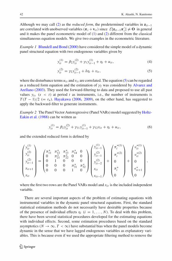
Example 2 The Panel Vector Autoregressive (Panel VARs) model suggested by Holtz-Eakin et al. (1988) can be written as
y(1)i t = β2 y(2)i t + γ11 y(1)i t−1 + γ12xit + ηi + uit , (6)
and the extended reduced form is defined by
⎛⎜⎜⎜⎜⎜⎜⎜⎜⎝
y(1)i t
y(2)i t
y(2)i t−1
xit+1
xit
⎞⎟⎟⎟⎟⎟⎟⎟⎟⎠
=
⎛⎜⎜⎜⎜⎝π∗
11 π∗12 π∗
13 π∗14 0
0 π∗21 π∗
22 0 00 1 0 0 00 0 0 π∗
31 π∗32
0 0 0 1 0
⎞⎟⎟⎟⎟⎠
⎛⎜⎜⎜⎜⎜⎜⎜⎜⎝
y(1)i t−1
y(2)i t−1
y(2)i t−2
xit
xit−1
⎞⎟⎟⎟⎟⎟⎟⎟⎟⎠
+
⎛⎜⎜⎜⎜⎜⎜⎜⎜⎝
π∗(1)i
π∗(2)i
0
π∗i
0
⎞⎟⎟⎟⎟⎟⎟⎟⎟⎠
+
⎛⎜⎜⎜⎜⎜⎜⎜⎜⎝
v∗(1)i t
v∗(2)i t
0
ε∗i t+1
0
⎞⎟⎟⎟⎟⎟⎟⎟⎟⎠,
where the first two rows are the Panel VARs model and xit is the included independentvariable.
There are several important aspects of the problem of estimating equations withinstrumental variables in the dynamic panel structural equations. First, the standardstatistical estimation methods do not necessarily have desirable properties becauseof the presence of individual effects ηi (i = 1, . . . , N ). To deal with this problem,there have been several statistical procedures developed for the estimating equationswith individual effects. Second, some estimation procedures based on the standardasymptotics (N → ∞, T < ∞) have substantial bias when the panel models becomedynamic in the sense that we have lagged endogenous variables as explanatory vari-ables. This is because even if we used the appropriate filtering method to remove the
123
The LIML approach to dynamic panel SEMs 43
individual effects, their influence cause the second-order bias through the past vari-ables and it becomes serious when T becomes large as Akashi and Kunitomo (2012)illustrated. Although we can remove the source of correlations among the laggedendogenous variables and heterogeneity of individual using the filtering procedure,we cannot remove the simultaneity by the standard procedure.
We shall develop a new statistical procedure which may overcome these problemsat the same time by applying the limited information maximum likelihood (PLIML)method. The asymptotic properties of the LIML method for estimating structural equa-tions including its asymptotic optimality have been recently investigated by Andersonet al. (2010, 2011) when there are many instruments. We extend their analysis to thePLIML method when the number of instruments increases as T , which may be quitenatural in the estimation problem of dynamic panel structural equations. Before weapply the LIML method, however, first we need to use the filtering procedure to theoriginal data, which is a data transformation. There are alternative filtering procedures,which correspond to either the forward direction filtering or the backward directionfiltering, to remove their individual effects.
2.2 Instrumental variables and filtering procedures
Let y(1)i = (y(1)i t ),Y(2)i = (y(2)′
i t ) and Z(1)i(−1) = (z(1)′
i t−1) be T × 1, T × G2 and T × K1matrices. We define the forward deviation operator A f , which is the (T − 1) × Tupper triangular matrix used by Arellano and Bover (1995) and Alvarez and Arellano(2003) such that A f A
′f = IT −1, ι = (1, . . . , 1)
′and A
′f A f = QT = IT − ιT ι
′T /T .
We apply the forward deviation operator y(1)i ,Y(2)i , and Z(1)i(−1) and then denote the
resulting variables as y(1, f )i = (y(1, f )
i t ),Y(2, f )i = (y(2, f )′
i t ) and Z(1, f )i = (z(1, f )′
i t−1 ). Foran example, we denote
y(2, f )i t = ct
[y(2)i t − 1
T − t(y(2)i t+1 + · · · + y(2)iT )
](7)
where c2t = (T − t)/(T − t + 1) for t = 1, . . . , T − 1, T ≥ 2. Using the forward-
filtered variables, we write for t = 1, . . . , T − 1 as
y(1, f )i t = β
′2 y(2, f )
i t + γ′1z(1, f )
i t−1 + u( f )i t , (8)
where u( f )i = (u( f )
i t ) is the transformed (T − 1)× 1 vector by u( f )i = A f ui from the
T ×1 disturbance vector ui = (uit ). Here, we have the relation that E[z(1, f )i t u( f )
i t ] �= 0,consequently.
We also define the backward operator Ab with the filter direction to the past, whichis the (T − 1) × T lower triangular matrix as used by Hayakawa (2006). This pro-cedure removes the individual effects from the instrumental variables. We denote thetransformed instrumental variables Z(b)i(−1) = (z(b)
′i t−1) and
123
44 K. Akashi, N. Kunitomo
z(b)i t−1 = bt
[zi t−1 − 1
t(zi t−2 + · · · + zi0 + zi(−1))
], (9)
where b2t = t/(t + 1) for t = 1, . . . , T − 1, and we include zi(−1) to simplify the
notation of the index range.The forward-filtering enables us to make use of the orthogonal conditions for the
disturbance terms. The backward-filtering removes the individual effects from instru-mental variables. In our analysis, we use two types of transformations on the instru-mental variables, and the instrumental matrices at period t are defined by
Z(a)t =
⎛⎜⎜⎜⎝
z(a)1(t−1) · · · z(a)N (t−1)
......
...
z(a)10 · · · z(a)N0
⎞⎟⎟⎟⎠
′
, Z(b)t =(
z(b)1(t−1), . . . , z(b)N (t−1)
)′, (10)
where z(a)i t−1 is the K∗ × 1 vector such that z(a)i t−1 = J′K∗zi t−1, and the selection matrix
J′K∗ chooses the nearest lagged variables to t − 1 while Z(b)t is the N × K matrix. The
dimension reduction from K to K∗ is often needed for the full rank of (Z(a)′
t Z(a)t ),
where Z(a)t is the N × (K∗t).We shall consider two alternative ways of the instrumental variables.(a) At period t , we use all available lagged variables after applying the forward-
filtering to the structural equation as suggested by Arellano and Bover (1995) andAlvarez and Arellano (2003). Since the instruments z(a)is (0 ≤ s < t) are generated bythe past information at t and the individual effects, the orthogonal conditions at periodt can be written as
E[z(a)is u( f )
i t
]= 0 (0 ≤ s < t ≤ T ). (11)
When T is large, the number of orthogonal conditions can be large if we use allorthogonal conditions imposed.
(b) Alternatively, at period t , we can use the only (a fixed number of) lagged variablesincluded in the reduced form after applying the backward-filtering to all instruments.Since the instruments z(b)is (0 ≤ s < t) are generated by the past information at t andthe individual effects are removed, the orthogonal conditions at period t used can bewritten as
E[z(b)i t−1u( f )
i t
]= 0,
which are the standard orthogonal conditions except the effects of the forward-filteringand backward-filtering for the original data.
Then, we consider two asymptotic sequences with respect to two dimensions Nand T in alternative ways. We define the total number of orthogonal conditions usedas rn and consider the ratio rn/n (the total sample N T (= n)) as
123
The LIML approach to dynamic panel SEMs 45
(a)K∗T (T − 1)
2N TN ,T →∞→ ca =
(K∗2
)lim
N ,T →∞
(T
N
). (12)
(b)K (T − 1)
N0TT →∞→ cb = K
N0, (13)
where we use the notation N (= N0) as a fixed integer. Then we shall investigate theasymptotic behaviors of estimators when the sequence of ratio can be a reasonableapproximation when rn and N are large under panel structural equation model. Whenthe number of instruments used is reduced to O(T ), the doubly-filtered LIML estima-tor does not need the double asymptotics N , T → ∞ and the number of individualsis regarded as a fixed number.
2.3 The LIML and GMM Estimation
Let y( f )t = (y(1, f )
i t , y(2, f )′i t )
′be (1 + G2) vectors and
Y( f )′t =
(y( f )
1t , . . . , y( f )Nt
), Z(1, f )′
t =(
z(1, f )1t , . . . , z(1, f )
Nt
),
be (1+G2)× N , and K1 × N matrices of the forward-filtered variables, respectively.Using these notations, we define two (1 + G2 + K1)× (1 + G2 + K1) matrices as
G( f ) =T −1∑t=1
(Y( f )′
t
Z(1, f )′t−1
)Mt
(Y( f )
t ,Z(1, f )t−1
), (14)
and
H( f ) =T −1∑t=1
(Y( f )′
t
Z(1, f )′t−1
)[IN − Mt ]
(Y( f )
t ,Z(1, f )t−1
), (15)
where the projection matrices Mt = M(a)t and M(b)
t are defined by M(a)t =
Z(a)t (Z(a)′
t Z(a)t )−1Z(a)′
t and M(b)t = Z(b)t (Z(b)
′t Z(b)t )−1Z(b)
′t . Then the LIML estima-
tor θ(.)
LI = (β′2.LI, γ
′1.LI)
′of (1,−β
′2,−γ
′1)
′ = (1,−θ ′)′ is defined by
[1
nG( f ) − λn
1
qnH( f )
][1
−θ(.)
LI
]= 0, (16)
where n = N T, qn = n − rn and λn is the smallest root of
∣∣∣∣1n G( f ) − l1
qnH( f )
∣∣∣∣ = 0. (17)
123
46 K. Akashi, N. Kunitomo
In this formulation, we use the notation θ(.)
LI = θ(a)LI in the case of M(a)
t and θ(b)LI in the
case of M(b)t , respectively. The solution to (16) gives the minimum of the variance
ratio
VRn =
[1,−θ
′]G( f )
[1−θ
][1,−θ
′]H( f )
[1−θ
] . (18)
Similarly, we define the panel GMM (or two-stage least squares TSLS) estimator,
θ(.)
G M = (β′2.G M , γ
′1.G M )
′of (1,−β
′2,−γ
′1)
′ = (1,−θ ′)′ by
[0, IG2+K1
] T −1∑t=1
[Y( f )′
t
Z(1, f )′t−1
]Mt
[Y( f )
t ,Z(1, f )t−1
] [1
−θ(.)
G M
]= 0 (19)
and we denote θ(a)G M and θ
(b)G M accordingly. It minimizes the numerator of the variance
ratio in (18). The LIML and TSLS estimation methods were originally developed byAnderson and Rubin (1949, 1950), and we modify them slightly to develop the panelLIML and the panel GMM (or TSLS) methods for the dynamic panel simultaneousequations model with individual effects.
3 Asymptotic properties of the LIML and GMM estimators
3.1 Asymptotic distributions
In this section, we shall derive the limiting distributions of the LIML and the GMMestimators when we have the representation y∗
i t = Π∗y∗i,t−1 + π∗
i + v∗i t and G∗ × 1
vector y∗i t includes yi t (1 + G2 ≤ G ≤ G∗). Then we shall investigate the case when
1 + G2 ≤ G ≤ G∗ when y∗i t can be degenerated as above and both Examples 1
and 2 are some special cases. There can be some possible ways of extensions of ourarguments, but then we would need quite lengthy derivations as Sect. 6 of this paperhas suggested.
Let wi t = y∗i t − μi and (IG∗ − Π∗)μi = π∗
i . We make a set of assumptions on themoments of disturbances and the dynamics of the underlying process {wi t } satisfying
wi t = Π∗wi t−1 + v∗i t . (20)
(A1) {v∗i t } (i = 1, . . . , N ; t = 1, . . . , T ) are i.i.d. across time and individuals and
independent of π∗i and zi0 with E[v∗
i t ] = 0, E[v∗i t v
∗′i t ] = Ω∗ and E[‖vi t‖8] exists.
(A2) The initial observation satisfies y∗i0 = (IG∗ − Π∗)−1π∗
i + wi0 (i =1, . . . , N ), where wi0 is independent of π∗
i and i.i.d. with the steady state dis-tribution of the homogenous process such that wi0 =∑∞
j=0 Π j vi,− j . All roots of∣∣Π∗ − λIG∗∣∣ = 0 satisfy the stationarity condition |λk | < 1 (k = 1, . . . ,G∗).
123
The LIML approach to dynamic panel SEMs 47
(A3) There exists an K∗ × 1 (K∗ ≤ K ) vector of instrumental variables zi,t−1 in(2) such that Z(a)t and Z(b)t in (10) are non-degenerate.
The assumptions (A1) and (A2) are analogous to some conditions used by Alvarezand Arellano (2003). They imply that the underlying processes for {yi t } and {wi t } arestationary. We shall make use of the assumption on initial condition to prove Lemmasin Sect. 6, but they could be relaxed at the expense of the resulting lengthy derivations.
To state main theoretical results in concise ways, we prepare some notations such
that E[vi t v′i t ] = Ω, σ 2 = E[u2
i t ] = β ′Ωβ, whereβ = (1,−β ′2)
′,u⊥i t = [0, IG2 ]
[vi t −
Cov(vi t , uit )uit/σ2],Φ∗ = D′J′
K E[wi(t−1)w′i(t−1)]JK D,D = (Π2, JK1) and J
′K1
=(IK1,O).
We first discuss Case (a) when we take the forward-filtering procedure and thenapply the LIML and the GMM estimation. We denote Mt = M(a)
t and we have thenext result whose proof will be in Sect. 6.
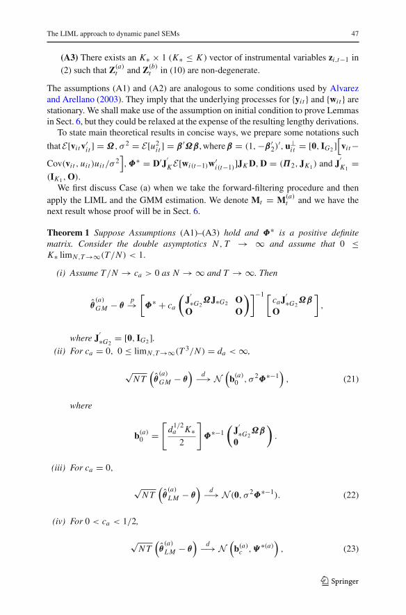
Theorem 1 Suppose Assumptions (A1)–(A3) hold and Φ∗ is a positive definitematrix. Consider the double asymptotics N , T → ∞ and assume that 0 ≤K∗ limN ,T →∞(T/N ) < 1.
(i) Assume T/N → ca > 0 as N → ∞ and T → ∞. Then
θ(a)G M − θ
p→[Φ∗ + ca
(J
′∗G2
ΩJ∗G2 OO O
)]−1 [caJ
′∗G2
Ωβ
O
],
where J′∗G2
= [0, IG2 ].(ii) For ca = 0, 0 ≤ limN ,T →∞(T 3/N ) = da < ∞,
√N T
(θ(a)G M − θ
)d−→ N
(b(a)0 , σ 2Φ∗−1
), (21)
where
b(a)0 =[
d1/2a K∗
2
]Φ∗−1
(J
′∗G2
Ωβ
0
).
(iii) For ca = 0,
√N T
(θ(a)L M − θ
)d−→ N (0, σ 2Φ∗−1). (22)
(iv) For 0 < ca < 1/2,
√N T
(θ(a)L M − θ
)d−→ N
(b(a)c ,Ψ ∗(a)) , (23)
123
48 K. Akashi, N. Kunitomo
where c∗a = ca/(1 − ca), J′G2
= (IG2 ,O),
Ψ ∗(a) = Φ∗−1[σ 2Φ∗ + JG2(ca[Ωσ 2 − Ωββ ′Ω]22 + Ξ
(a)4 )J
′G2
]Φ∗−1,
[ · ]22 is the (2,2)-th element (G2 × G2 matrix) of the partitioned (1+ G2)× (1+ G2)
matrix,
Ξ(a)4 =
(1
1 − ca
)2
E[(
u2i t − σ 2
)u⊥
i t u⊥′i t
] [plimN ,T →∞
1
N T
T −1∑t=1
d(a)′
t d(a)t − c2a
],
b(a)c = −(
K∗2
)1/2 c1/2a
(1 − ca)Φ∗−1D′J′
G∗(IG∗ − Π∗)−1E [v∗i t uit
],
d(a)t = (d(a)i t ) = diag(M(a)t ) and Wt−1 = (w1(t−1), . . . ,wN (t−1))
′ is the N × K∗matrix consisting of {wi t }.
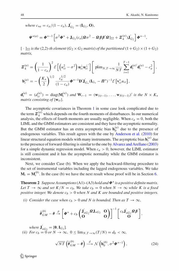
The asymptotic covariances in Theorem 1 in some case look complicated due tothe term Ξ
(a)4 which depends on the fourth moments of disturbances. In our numerical
analysis, the effects of fourth moments are usually negligible. When ca = 0, both theLIML and the GMM estimators are consistent and they have the asymptotic normality.But the GMM estimator has an extra asymptotic bias b(a)0 due to the presence ofendogenous variables. This result agrees with the one by Anderson et al. (2010) forlinear structural equation models with many instruments. The asymptotic bias b(a)c dueto the presence of forward-filtering is similar to the one by Alvarez and Arellano (2003)for a simple dynamic regression model. When ca > 0, however, the LIML estimatoris still consistent and it has the asymptotic normality while the GMM estimator isinconsistent.
Next, we consider Case (b). When we apply the backward-filtering procedure tothe set of instrumental variables including the lagged endogenous variables. We takeMt = M(b)
t . In the case (b) we have the next result whose proof will be in Section 6.
Theorem 2 Suppose Assumptions (A1)–(A3) hold andΦ∗ is a positive definite matrix.Let T → ∞ and set K/N = cb. We take cb = 0 when N → ∞ while K is a fixedpositive integer. We denote cb > 0 when N and K are bounded and positive integers.
(i) Consider the case when cb > 0 and N is bounded. Then as T → ∞,
θ(b)G M − θ
p→[Φ∗ + cb
(J
′∗G2
ΩJ∗G2 OO O
)]−1 [cbJ
′∗G2
Ωβ
O
],
where J′∗G2
= [0, IG2 ].(ii) For cb = 0 or N → ∞, 0 ≤ limN ,T →∞(T/N ) = db < ∞,
√N T
(θ(b)G M − θ
)d−→ N
(b(b)0 , σ 2Φ∗−1
), (24)
123
The LIML approach to dynamic panel SEMs 49
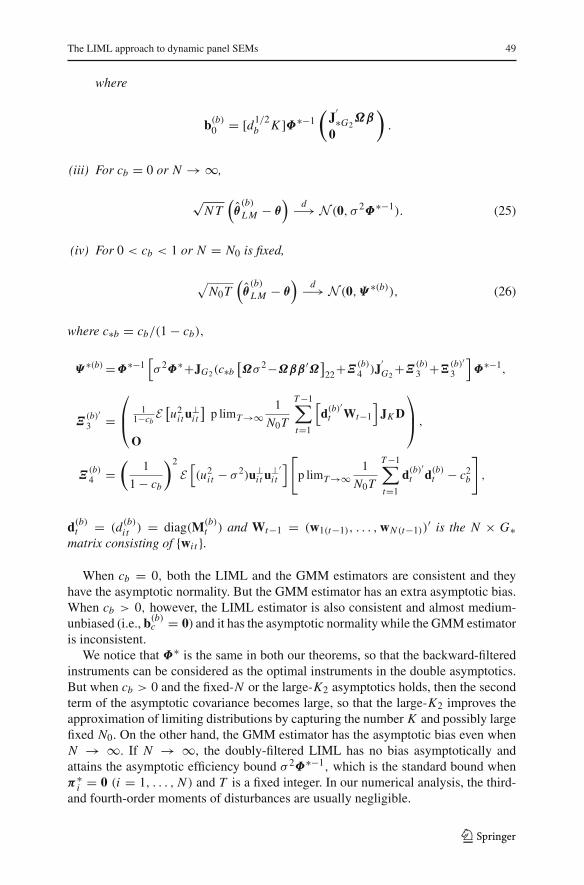
where
b(b)0 = [d1/2b K ]Φ∗−1
(J
′∗G2
Ωβ
0
).
(iii) For cb = 0 or N → ∞,
√N T
(θ(b)L M − θ
)d−→ N (0, σ 2Φ∗−1). (25)
(iv) For 0 < cb < 1 or N = N0 is fixed,
√N0T
(θ(b)L M − θ
)d−→ N (0,Ψ ∗(b)), (26)
where c∗b = cb/(1 − cb),
Ψ ∗(b)=Φ∗−1[σ 2Φ∗+JG2(c∗b
[Ωσ 2−Ωββ ′Ω
]22+Ξ
(b)4 )J
′G2
+Ξ(b)3 +�
(b)′3
]Φ∗−1,
Ξ(b)′3 =
⎛⎜⎝ 1
1−cbE [u2
i t u⊥i t
]p limT →∞
1
N0T
T −1∑t=1
[d(b)
′t Wt−1
]JK D
O
⎞⎟⎠ ,
Ξ(b)4 =
(1
1 − cb
)2
E[(u2
i t − σ 2)u⊥i t u⊥′
i t
] [p limT →∞
1
N0T
T −1∑t=1
d(b)′
t d(b)t − c2b
],
d(b)t = (d(b)i t ) = diag(M(b)t ) and Wt−1 = (w1(t−1), . . . ,wN (t−1))
′ is the N × G∗matrix consisting of {wi t }.
When cb = 0, both the LIML and the GMM estimators are consistent and theyhave the asymptotic normality. But the GMM estimator has an extra asymptotic bias.When cb > 0, however, the LIML estimator is also consistent and almost medium-unbiased (i.e., b(b)c = 0) and it has the asymptotic normality while the GMM estimatoris inconsistent.
We notice that Φ∗ is the same in both our theorems, so that the backward-filteredinstruments can be considered as the optimal instruments in the double asymptotics.But when cb > 0 and the fixed-N or the large-K2 asymptotics holds, then the secondterm of the asymptotic covariance becomes large, so that the large-K2 improves theapproximation of limiting distributions by capturing the number K and possibly largefixed N0. On the other hand, the GMM estimator has the asymptotic bias even whenN → ∞. If N → ∞, the doubly-filtered LIML has no bias asymptotically andattains the asymptotic efficiency bound σ 2Φ∗−1, which is the standard bound whenπ∗
i = 0 (i = 1, . . . , N ) and T is a fixed integer. In our numerical analysis, the third-and fourth-order moments of disturbances are usually negligible.
123
50 K. Akashi, N. Kunitomo
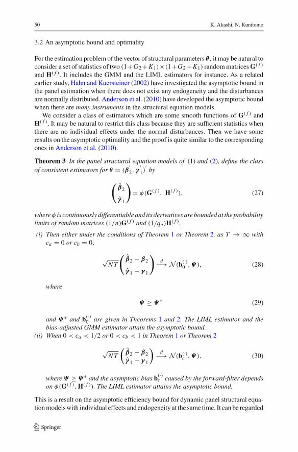
3.2 An asymptotic bound and optimality
For the estimation problem of the vector of structural parameters θ, it may be natural toconsider a set of statistics of two (1+G2 +K1)×(1+G2 +K1) random matrices G( f )
and H( f ). It includes the GMM and the LIML estimators for instance. As a relatedearlier study, Hahn and Kuersteiner (2002) have investigated the asymptotic bound inthe panel estimation when there does not exist any endogeneity and the disturbancesare normally distributed. Anderson et al. (2010) have developed the asymptotic boundwhen there are many instruments in the structural equation models.
We consider a class of estimators which are some smooth functions of G( f ) andH( f ). It may be natural to restrict this class because they are sufficient statistics whenthere are no individual effects under the normal disturbances. Then we have someresults on the asymptotic optimality and the proof is quite similar to the correspondingones in Anderson et al. (2010).
Theorem 3 In the panel structural equation models of (1) and (2), define the classof consistent estimators for θ = (β
′2, γ
′1)
′by
(β2
γ 1
)= φ(G( f ), H( f )), (27)
whereφ is continuously differentiable and its derivatives are bounded at the probabilitylimits of random matrices (1/n)G( f ) and (1/qn)H( f ).
(i) Then either under the conditions of Theorem 1 or Theorem 2, as T → ∞ withca = 0 or cb = 0,
√N T
(β2 − β2
γ 1 − γ 1
)d−→ N (b(·)0 ,Ψ ), (28)
where
Ψ ≥ Ψ ∗ (29)
and Ψ ∗ and b(·)0 are given in Theorems 1 and 2. The LIML estimator and thebias-adjusted GMM estimator attain the asymptotic bound.
(ii) When 0 < ca < 1/2 or 0 < cb < 1 in Theorem 1 or Theorem 2
√N T
(β2 − β2γ 1 − γ 1
)d−→ N (b(·)c ,Ψ ), (30)
where Ψ ≥ Ψ ∗ and the asymptotic bias b(·)c caused by the forward-filter dependson φ(G( f ),H( f )). The LIML estimator attains the asymptotic bound.
This is a result on the asymptotic efficiency bound for dynamic panel structural equa-tion models with individual effects and endogeneity at the same time. It can be regarded
123
The LIML approach to dynamic panel SEMs 51
as an extension of Theorem 4 of Anderson et al. (2010) for the linear structural equa-tion in the simultaneous equation systems. Because of individual effects in the panelstructural equations and the filtering problem, there are additional features on theasymptotic optimality.
4 On finite sample properties
It is important to investigate the finite sample properties of estimators partly becausethey are not necessarily similar to their asymptotic properties. One simple examplewould be the fact that the exact moments of some estimators do not necessarily exist. Inthat case, it may be meaningless to compare the exact MSEs of alternative estimatorsand their Monte Carlo analogs.
In our experiments, we took Example 2 (K = 4, K∗ = 3, K1 = 2,G2 = 1) inSect. 2 as a typical example.1 In Example 2 we set the unknown parameters suchas (β2, γ11) = (.5, .5), γ12 = .3, and (ω11, ω12, ω22) = (1.0, .3, 1.0), (1.5, 1.0, 1.0)where we take γ 1 = (γ11, γ12)
′and Ω = (ωi j ). Also we control the variance of each
components of π i as 1. Our experiments are similar to the ones reported in Akashi(2008), and Akashi and Kunitomo (2012). Then we generate a large number of randomvariables by simulations and calculate the empirical distribution functions of the GMMand LIML estimators in their normalized forms. We repeat 5,000 replications for eachcase and the smoothing technique to estimate the empirical distribution functions.The details of simulations are similar to those explained by Anderson et al. (2005,2011). We report only the results for (N , T ) = (100, 25) and (100, 50) as the typicalcases among a large number of our simulations. All simulations reported in this sectionhave been done under the situation that the disturbance terms are normally distributed.Although we have done a number of simulations when the disturbances are non-normalsuch as the t-distribution, we have omitted them to save space because they are quitesimilar to the results reported.
We examine the distribution functions of the LIML and GMM estimators in twonormalizations. The first one is in terms of
√N T
σ
[(φ11)−1/2 00 (φ22)−1/2
] [β2 − β2γ1 − γ1
], (31)
where φ11 and φ22 are the (1,1)-th element and (2.2)-th element of Φ∗−1, respectively.The second normalization is
√N T
[ψ
−1/211 0
0 ψ−1/222
][(β2 − β2γ1 − γ1
)− 1√
N Tb(·)c
], (32)
where b(·)c is the asymptotic bias term, ψ11 and ψ22 are the (1,1)-th element and the(2,2)-th element of Ψ ∗, respectively. We have chosen these standardizations because
1 We have used Example 1 in Akashi and Kunitomo (2012) to investigate Case (a) in more details. Example 1can be regarded as a special case of Example 2.
123
52 K. Akashi, N. Kunitomo
of the form of the limiting distribution of the LIML estimator in Theorems 1 and 2.We may call the large-rn case when c = 0 (c = ca or cb) and c �= 0 as the generalcase.
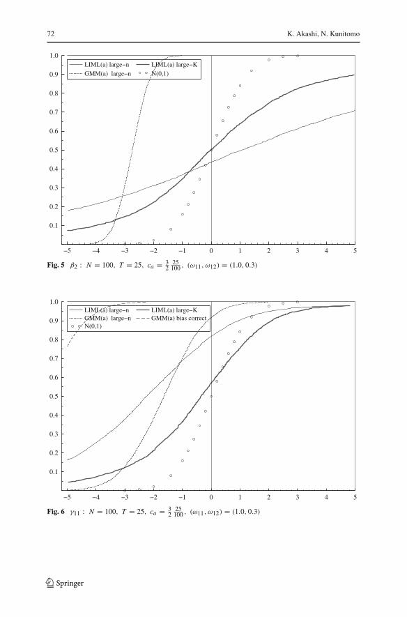
Since Akashi and Kunitomo (2012) have given many figures on Case (a), we onlygive Figs. 5 and 6 in Appendix. We have shown the estimated distribution functionsof the GMM and the LIML estimators of (β2, γ1) and we confirm the findings ofAkashi and Kunitomo (2012) in a simple case. The GMM estimator is badly biasedwhen N and T are large while the LIML estimator is almost median-unbiased aftercorrecting the bias term in (32). However, the normalization by the limiting covariancematrix of the LIML estimator when c = 0 is not appropriate. This aspect can beobserved because the circles in figures are the standard normal distribution functionN(0,1).
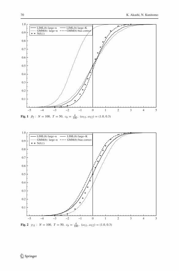
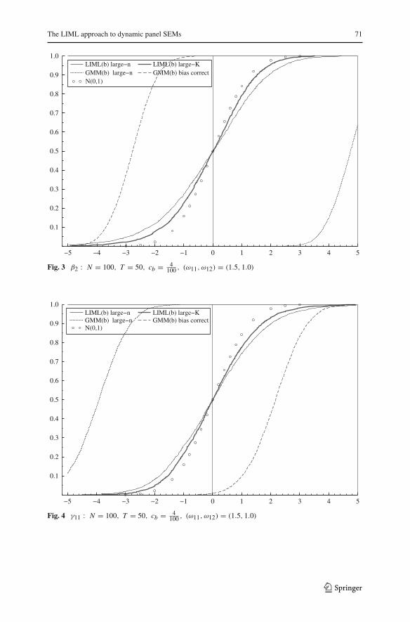
For Case (b) with the backward-filtering procedure, we show the estimated distri-bution functions of the GMM and LIML estimators of β2 and γ1 as Figs. 1, 2, 3 and4 among many results. From these figures, we first observe that the GMM estimatoris often biased when N and T are large while the LIML estimator is almost median-unbiased. Second, the normalization by the limiting covariance matrix of the LIMLestimator when c = 0 is often not appropriate. Since the normal approximations basedon the general case c �= 0, it is important to use the formulas in Sect. 3.
5 Conclusions
In this paper, we develop the panel-limited information maximum likelihood (PLIML)approach for estimating dynamic panel simultaneous equation models. When there aredynamic effects and endogenous variables with individual effects at the same time,the LIML method for the filtered data does give not only the consistency and theasymptotic normality, but also attains the asymptotic efficiency bound when the orderof orthogonal conditions is large or many instruments.
The consistency of LIML method does not depend on specified panel asymptoticsand the total number of instruments as long as it is less than the total number ofobservations. The approximation of its limiting distribution embodies the influence ofthe number of instrumental variables automatically and our method gives an unifiedapproach for solving the statistical problem with panel data when N and T are large.
We have examined the effects of alternative filtering procedures. When we onlyapply the forward-filtering and use O(T 2) instruments, the GMM estimator is badlybiased while the LIML estimator can be almost-unbiased. If we use the backward-filtering to instruments, the GMM estimator is often biased, but its magnitude is sig-nificantly reduced. Since we often do not know the precise form of lag structures ofthe reduced form in the panel simultaneous equation models, we conclude that theLIML method has the asymptotic robustness in both cases of (a) and (b) while theGMM does not have such robustness.
In a companion paper, Akashi and Kunitomo (2012) have investigated the finitesample properties of alternative estimation methods such as the WG (Within Groups),the GMM and the PLIML estimators in a simpler setting. Although they have useda particular case of dynamic panel models and the forward filtering procedure, their
123
The LIML approach to dynamic panel SEMs 53
results are relevant for more general panel structural equations. In this sense, the LIMLmethod is quite useful and relevant in dynamic panel econometric modeling.
Finally, there is an important issue on the individual heteroscedasticity in panelstructural equation models. An optimal modification of the LIML method to removethe possible bias due to individual heteroscedasticity can be developed. The detailshave been discussed in Kunitomo and Akashi (2010), which was along the argumentsoriginally developed by Kunitomo (2012).
6 Mathematical details
In this section, we give the proofs of Theorems 1 and 2. The method of proofs are similarto those used in Akashi and Kunitomo (2012). When we use notations (Mt ,Nt , c, c∗),the relevant derivations are valid for each case of Mt = M(a)
t and M(b)t under the
corresponding asymptotics. (We shall use c and c∗ (= c/(1 − c)) for ca, cb (, whichare different from ct ), and c∗a (= ca/(1 − ca)), c∗b (= cb/(1 − cb)) without anyconfusion.) Also we use notations J for JK and zi t = Jwi,t−1, which means that therelevant information is in the first K -variables for the sake of convenience. Becausesome derivations have been given in Akashi and Kunitomo (2012) when G2 = 1 andit is often straight-forward to extend their analysis to the general case, we refer to theirresults in such cases.
Derivations of Theorems 1 and 2Step 1: First, we shall investigate the effects of the forward-filtering. We drive theprobability limits of sample quantities and obtain the representations for the LIMLestimator. Substitution of (7) into (14) yields
G( f ) = G( f,1) + G( f,2) + G( f,2)′ + G( f,3), (33)
where G( f,1) = D∗′ ∑T −1t=1 Z( f )′
t−1 Mt Z( f )t−1D∗,G( f,2) = D∗′ ∑T −1
t=1 Z( f )′t−1 Mt (V
( f )t ,O),
G( f,3) = ∑T −1t=1 (V
( f )t ,O)
′Mt (V
( f )t ,O),V( f )′
t = (v( f )1t , . . . , v( f )
Nt ) and v( f )i t (i =
1, . . . , N ) are the corresponding forward-filtered disturbances of vi t , and a K × (1 +G1 + K1) matrix D∗ = D[θ , IG2+K1 ].
We shall show that for Mt = M(a)t or M(b)
t ,
1
nG( f ) p−→ G0 =
[θ
′
IG2+K1
]Φ∗ [ θ , IG2+K1
]+ c
[Ω O
O O
](34)
and
1
qnH( f ) p−→ H0 =
[Ω O
O O
], (35)
123
54 K. Akashi, N. Kunitomo
where Φ∗ = D′J′E[wi t−1w′i t−1]JD = D′J′ 0JD and n = N T . Using the represen-
tation
(Y( f )′
t
Z(1, f )′t−1
)= D∗′
Z( f )′t−1 +
(V( f )′
t
O′
)(say, )
we show that (1/n)G( f,2) p→ OG2+K1 using the same argument for (1/√
n)∑T −1
t=1
Z( f )′t−1 Mt u
( f )t in Akashi and Kunitomo (2012). We write
Z( f )′t−1 = J
⎛⎝ct
⎡⎣IG∗ − 1
T − t
⎛⎝T −t∑
j=1
Π∗ j
⎞⎠⎤⎦W
′t−1 − ct V
′tT
⎞⎠ = Ψ t W
′t−1 − ct V
′tT ,
where V′tT is defined in Step 3 below. We further decompose (1/n)G( f,1) as
1
n
T −1∑t=1
Z( f )′t−1 Mt Z
( f )t−1 = 1
n
T −1∑t=1
Ψ t W′t−1Mt Wt−1Ψ
′t − 1
n
T −1∑t=1
ctΨ t W′t−1Mt VtT
−1
n
T −1∑t=1
ct V′tT Mt Wt−1Ψ
′t + 1
n
T −1∑t=1
c2t V
′tT Mt VtT . (36)
Moreover, using Lemmas 2 and 3 in Steps 4 and 5, and c2t = 1 − 1/(T − t + 1) after
some calculations, it is possible to show
1
n
T −1∑t=1
Ψ t W′t−1Mt Wt−1Ψ
′t
= 1
n
T −1∑t=1
c2t W
′t−1Mt Wt−1
− 1
n
T −1∑t=1
c2t
T − tW
′t−1Mt Wt−1
⎛⎝T −t∑
j=1
Π∗ j
⎞⎠
′
− 1
n
T −1∑t=1
c2t
T − t
⎛⎝T −t∑
j=1
Π∗ j
⎞⎠W
′t−1Mt Wt−1
+ 1
n
T −1∑t=1
(ct
T − t
)2⎛⎝T −t∑
j=1
Π∗ j
⎞⎠W
′t−1Mt Wt−1
⎛⎝T −t∑
j=1
Π∗ j
⎞⎠
′
(37)
converges to E[wi(t−1)w′i(t−1)] in probability. The second and third terms of (36) have
zero means and their variances to tend to zeros. It is because
123
The LIML approach to dynamic panel SEMs 55
Var
[1
N T
T −1∑t=1
ct e′jΨ t W
′t−1Mt VtT ek
]
≤ 1
N 2T 2
T −1∑t=1
T −1∑s=1
√c2
t E[(e
′jΨ t W
′t−1Mt VtT ek)2
]√c2
s E[(e
′kVsT MsWs−1Ψ
′se j )2
],
where e j ( j, k = 1, . . . , K ) are j-th unit vector. Also we have
c2t E[(e
′jΨ t W
′t−1Mt VtT ek)
2]= c2
t
[e
′kE[vi tT v
′i tT
]ek
]E[e
′jΨ t W
′t−1Mt Wt−1Ψ
′t e j
]
≤ c2t
[1
(T − t)2e
′k
T −t∑h=1
ΦhE[v∗
i0v∗′i0
]Φ
′hek
]
×[e
′jΨ tE[W′
t−1Wt−1]Ψ ′t e j
],
which is O(N/(T − t)) because∑T −t
h=1 e′kΦhE[v∗
i0v∗′i0]Φ
′hek = O(T − t). Then
Var
[1
N0
T −1∑t=1
ct e′jΨ t W
′t−1Mt VtT ek
]= O
((√
T )2
N0T 2
).
For the fourth term of (36), the expected value is given by
E[
1
n
T −1∑t=1
c2t e
′j V
′tT Mt VtT ek
]= 1
n
T −1∑t=1
c2t tr(Mt )E
[e
′j vi tT v
′i tT ek
]
= O
(1
n
∑t
tr(Mt )
T − t + 1
)
and it converges to zero in probability. Its variance tends to zero in the same way asfor ϒ(k)21n and ϒ(k)22n in Step 3 below.
Next, we consider (1/n)G( f,3). Using the fact that Et [v( f )i t v( f )′
i t ] = Ω ,
E[
1
n
T −1∑t=1
e′gV( f )′
t Mt V( f )t eh
]= e
′gΩeh
n
T −1∑t=1
tr(Mt ),
which converges to c(e′gΩeh) as n → ∞. Moreover, using V( f )
t = (Vt − VtT )/ct ,we decompose
123
56 K. Akashi, N. Kunitomo
1
n
T −1∑t=1
V( f )′t Mt V
( f )t = 1
n
T −1∑t=1
c−2t V
′t Mt Vt − 1
n
T −1∑t=1
c−2t V
′t Mt VtT
−1
n
T −1∑t=1
c−2t V
′tT Mt Vt + 1
n
T −1∑t=1
c−2t V
′t Mt VtT . (38)
Because of Lemma 1 of Step 3 below, Var[v(g)′t Mt v(h)t ] = O(t) and Cov[v(g)′t Mt v
(h)t ,
v(g)′
s Mt v(h)s ] = 0 for t �= s. Hence the variance of the first term satisfies
Var
[1
n
T −1∑t=1
e′gV( f )′
t Mt V( f )t eh
]= 1
n2
T −1∑t=1
(1 + 1
T − t
)2
× O(t),
which converges to zero.The second and third terms of the right-hand side of (38) can be evaluated analo-
gously asϒ(k)21n andϒ(k)22n , and their variances tend to zeros using the similar arguments.
We turn to show that (1/qn)H( f ) p→ H0 by evaluating
1
n
T −1∑t=1
(Y( f )′
t
Z(1, f )′t−1
)(Y( f )
t ,Z(1, f )t−1 )
= D∗′ 1
n
T −1∑t=1
Z( f )′t−1 Z( f )
t−1D∗ + D∗′ 1
n
T −1∑t=1
Z( f )′t−1 (V
( f )t ,O)
+1
n
T −1∑t=1
(V( f )′
tO′
)Z( f )
t−1D∗ + 1
n
T −1∑t=1
(V( f )′
tO′
)(V( f )
t ,O). (39)
The expected values of the second and third terms of 1/(N0T )∑
t E[Z( f )′t−1 V( f )
t ] =(1/T )(IG∗ −Π∗)−1E[v∗
i t v∗′i t ]+O(1/T ) converge to zeros as T → ∞. We can establish
the mean squared convergence similarly. Moreover,
1
n
T −1∑t=1
e′j Z( f )′t−1 Z( f )
t−1ek = 1
N0T
N0∑i=1
T −1∑t=1
w( j)i(t−1)w
(k)i(t−1)−
1
N0T
N0∑i=1
1
Tι′T w( j)
i(t−1)w(k)′i(t−1)ιT
converges to E[w( j)i(t−1)w
(k)i(t−1)] in probability since (1/T )
∑T −1t=1 w
( j)i(t−1)w
(k)i(t−1)
p→E[w( j)
i(t−1)w(k)i(t−1)] and the second term converges to (1/N0)
∑N0i=1(0+op(1))2 = op(1)
using that (1/T )ι′T w( j)i(t−1)
p→ 0. Again using the similar argument, we have that
(1/n)∑T −1
t=1 V( f )′t V( f )
tp→ Ω . Hence
123
The LIML approach to dynamic panel SEMs 57
1
qnH( f ) p→ 1
1 − c
[plimn→∞
1
n
T −1∑t=1
(Y( f )′
t
Z(1, f )′t−1
)(Y( f )
t ,Z(1, f )t−1 )− G0
]= H0.
Step 2: Using the convergence results in Step 1, we have
∣∣∣∣Φθ + [c − (plimn→∞λn)]
[Ω OO O
]∣∣∣∣ = 0, (40)
where
Φθ =[
θ ′IG2+K1
]Φ∗ [θ , IG2+K1
]. (41)
By the assumption that Φ∗ is a positive definite matrix, λnp→ c and we have that
θLIp→ θ because (16) gives Φ∗(θ − θ) = op(1) . Define G( f )
1 = √n[(1/n)G( f ) −
G0],H( f )1 = √
qn[(1/qn)H( f ) − H0], λ( f )1n = √
n[λn − c] and b1 = √n[θ − θ ] . By
substituting these variables into (16), we find
[G0 − cH0][
1−θ
]+ 1√
n
[G( f )
1 − λ( f )1n H0
] [1−θ
]+ 1√
n[G0 − cH0] b1
− 1√qn
[cH( f )1 ]
[1−θ
]= op
(1√n
). (42)
Then using the relation of Φθ (1,−θ ′)′ = 0, we have
Φθ
[0b1
]=[G( f )
1 − λ( f )1n H0 − √
cc∗H( f )1
] [ 1−θ
]+ op(1).
Multiplication of (42) from the left by (1,−θ) yields
λ( f )1n =
(1,−θ ′)[G( f )
1 − √cc∗H( f )
1
](1,−θ ′)′
(1,−θ ′)H0(1,−θ ′)′+ op(1). (43)
Also the multiplication of (43) from the left by (0, IG2+K1) and substitution for λ( f )1n
for (43) yields
Φ∗√n
[β2L I − β2γ 1L I − γ 1
]
= [0, IG2+K1 ][
I1+G2+K1 − 1
β ′Ωβ
(Ωβ
0
)(1,−θ ′)
] [G( f )
1 −√cc∗H( f )
1
] [1−θ
]+op(1). (44)
123
58 K. Akashi, N. Kunitomo
Using the relation of (33), we have
[G( f )
1 − √cc∗H( f )
1
] [1−θ
]
= 1√n
D∗′T −1∑t=1
Z( f )′t−1 Mt u
( f )t + 1√
n
[T −1∑t=1
(V( f )′
tO
)Mt u
( f )t − rn
(Ωβ
0
)]
−√
cc∗√qn
D∗′T −1∑t=1
Z( f )′t−1 [IN − Mt ] u( f )
t
−√
cc∗√qn
[T −1∑t=1
(V( f )′
tO
)[IN − Mt ]u( f )
t − qn
(Ωβ
0
)]. (45)
Also we use the relations√
cc∗/√
qn−c∗/√
n = o(1), [I1+G2−(1/σ 2)Ωββ ′]Ωβ = 0and then
Φ∗√n
(β2L I − β2γ 1L I − γ 1
)= 1√
nD′
T −1∑t=1
Z( f )′t−1 Nt u
( f )t + 1√
n
T −1∑t=1
(U(⊥, f )′
tO
)Nt u
( f )t
+op(1). (46)
where Nt = Mt − c∗(IN − Mt ) = 11−c [Mt − cIN ] and
U(⊥, f )′t = [0, IG2
] [I1+G2 − Ωββ
′
β′Ωβ
]V( f )′
t =(
u(⊥, f )1t , . . . ,u(⊥, f )
Nt
).
Step 3: We evaluate the additional effects of the forward-filtering on the LIMLestimation at this step by setting Mt = M(a)
t and the k-th unit vector as ek =(0, . . . , 0, 1, 0, . . . , 0)′. Using (A2) and u( f )
t = (ut − utT )/ct , we decompose thefirst and second terms of (46) as, for k = 1, . . . , K (= K1 + K2) and g = 1, . . . ,G2,
1√n
T −1∑t=1
e′kZ( f )′
t−1 N(a)t u( f )t
= 1
1 − ca
[(1√n
T −1∑t=1
e′kJ′W′
t−1Mt ut − ϒ(k,a)11n −ϒ
(k,a)12n
)−(ϒ(k,a)21n − ϒ
(k,a)22n
)]
−c∗a
(1√n
T −1∑t=1
e′kJ′W′
t−1ut − ϒ(k)3n
), (47)
123
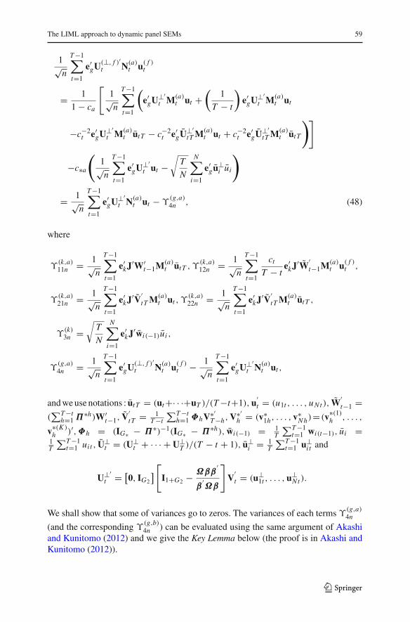
The LIML approach to dynamic panel SEMs 59
1√n
T −1∑t=1
e′gU(⊥, f )′
t N(a)t u( f )t
= 1
1 − ca
[1√n
T −1∑t=1
(e′
gU⊥′t M(a)
t ut +(
1
T − t
)e′
gU⊥′t M(a)
t ut
−c−2t e′
gU⊥′t M(a)
t utT − c−2t e′
gU⊥′tT M(a)
t ut + c−2t e′
gU⊥′tT M(a)
t utT
)]
−c∗a
(1√n
T −1∑t=1
e′gU⊥′
t ut −√
T
N
N∑i=1
e′gu⊥
i ui
)
= 1√n
T −1∑t=1
e′gU⊥′
t N(a)t ut − ϒ(g,a)4n , (48)
where
ϒ(k,a)11n = 1√
n
T −1∑t=1
e′kJ′W′
t−1M(a)t utT , ϒ
(k,a)12n = 1√
n
T −1∑t=1
ct
T − te′
kJ′W′t−1M(a)
t u( f )t ,
ϒ(k,a)21n = 1√
n
T −1∑t=1
e′kJ′V′
tT M(a)t ut , ϒ
(k,a)22n = 1√
n
T −1∑t=1
e′kJ′V′
tT M(a)t utT ,
ϒ(k)3n =
√T
N
N∑i=1
e′kJ′wi(−1)ui ,
ϒ(g,a)4n = 1√
n
T −1∑t=1
e′gU(⊥, f )′
t N(a)t u( f )t − 1√
n
T −1∑t=1
e′gU⊥′
t N(a)t ut ,
and we use notations : utT = (ut +· · ·+uT )/(T −t+1),u′t = (u1t , . . . , uNt ), W
′t−1 =
(∑T −t
h=1 Π∗h)W′t−1, V
′tT = 1
T −t
∑T −th=1 ΦhV∗′
T −h,V∗′h = (v∗
1h, . . . , v∗Nh)= (v∗(1)
h , . . . ,
v∗(K )h )′,Φh = (IG∗ − Π∗)−1(IG∗ − Π∗h), wi(−1) = 1
T
∑T −1t=1 wi(t−1), ui =
1T
∑T −1t=1 uit , U⊥
t = (U⊥t + · · · + U⊥
T )/(T − t + 1), u⊥i = 1
T
∑T −1t=1 u⊥
i t and
U⊥′t = [0, IG2
] [I1+G2 − Ωββ
′
β′Ωβ
]V
′t = (u⊥
1t , . . . ,u⊥Nt ).
We shall show that some of variances go to zeros. The variances of each terms ϒ(g,a)4n
(and the corresponding ϒ(g,b)4n ) can be evaluated using the same argument of Akashiand Kunitomo (2012) and we give the Key Lemma below (the proof is in Akashi andKunitomo (2012)).
123
60 K. Akashi, N. Kunitomo
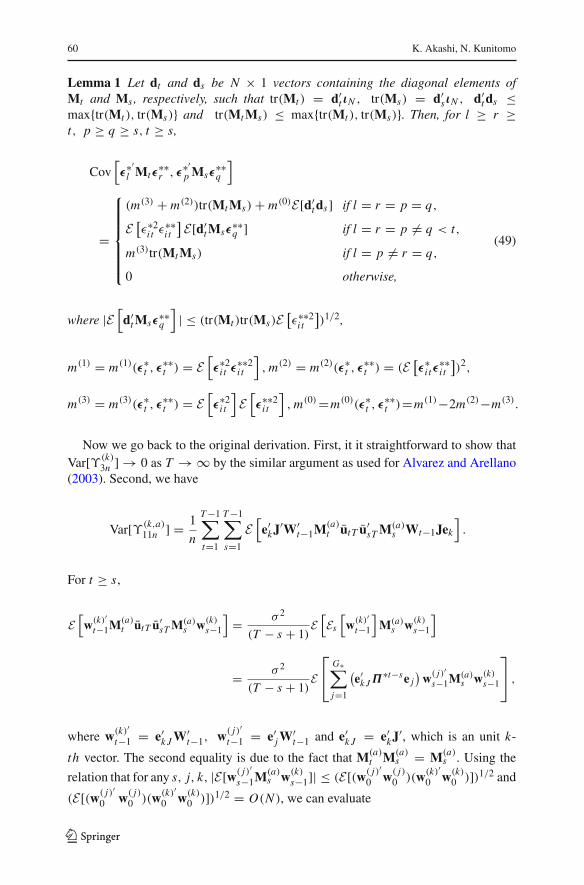
Lemma 1 Let dt and ds be N × 1 vectors containing the diagonal elements ofMt and Ms , respectively, such that tr(Mt ) = d′
t ιN , tr(Ms) = d′sιN , d′
t ds ≤max{tr(Mt ), tr(Ms)} and tr(Mt Ms) ≤ max{tr(Mt ), tr(Ms)}. Then, for l ≥ r ≥t, p ≥ q ≥ s, t ≥ s,
Cov[ε∗′
l Mtε∗∗r , ε
∗′p Msε
∗∗q
]
=
⎧⎪⎪⎪⎪⎪⎨⎪⎪⎪⎪⎪⎩
(m(3) + m(2))tr(Mt Ms)+ m(0)E[d′t ds] if l = r = p = q,
E [ε∗2i t ε
∗∗i t
] E[d′t Msε
∗∗q ] if l = r = p �= q < t,
m(3)tr(Mt Ms) if l = p �= r = q,
0 otherwise,
(49)
where |E[d′
t Msε∗∗q
]| ≤ (tr(Mt )tr(Ms)E
[ε∗∗2
i t
])1/2,
m(1) = m(1)(ε∗t , ε
∗∗t ) = E
[ε∗2
i t ε∗∗2i t
],m(2) = m(2)(ε∗
t , ε∗∗t ) = (E [ε∗
i tε∗∗i t
])2,
m(3) = m(3)(ε∗t , ε
∗∗t ) = E
[ε∗2
i t
]E[ε∗∗2
i t
],m(0)=m(0)(ε∗
t , ε∗∗t )=m(1)−2m(2)−m(3).
Now we go back to the original derivation. First, it it straightforward to show thatVar[ϒ(k)3n ] → 0 as T → ∞ by the similar argument as used for Alvarez and Arellano(2003). Second, we have
Var[ϒ(k,a)11n ] = 1
n
T −1∑t=1
T −1∑s=1
E[e′
kJ′W′t−1M(a)
t utT u′sT M(a)
s Wt−1Jek
].
For t ≥ s,
E[w(k)′
t−1M(a)t utT u′
sT M(a)s w(k)
s−1
]= σ 2
(T − s + 1)E[Es
[w(k)′
t−1
]M(a)
s w(k)s−1
]
= σ 2
(T − s + 1)E⎡⎣ G∗∑
j=1
(e′
k J Π∗t−se j)
w( j)′s−1M(a)
s w(k)s−1
⎤⎦ ,
where w(k)′t−1 = e′
k J W′t−1, w( j)′
t−1 = e′j W
′t−1 and e′
k J = e′kJ′, which is an unit k-
th vector. The second equality is due to the fact that M(a)t M(a)
s = M(a)s . Using the
relation that for any s, j, k, |E[w( j)′s−1M(a)
s w(k)s−1]| ≤ (E[(w( j)′
0 w( j)0 )(w(k)′
0 w(k)0 )])1/2 and
(E[(w( j)′0 w( j)
0 )(w(k)′0 w(k)
0 )])1/2 = O(N ), we can evaluate
123
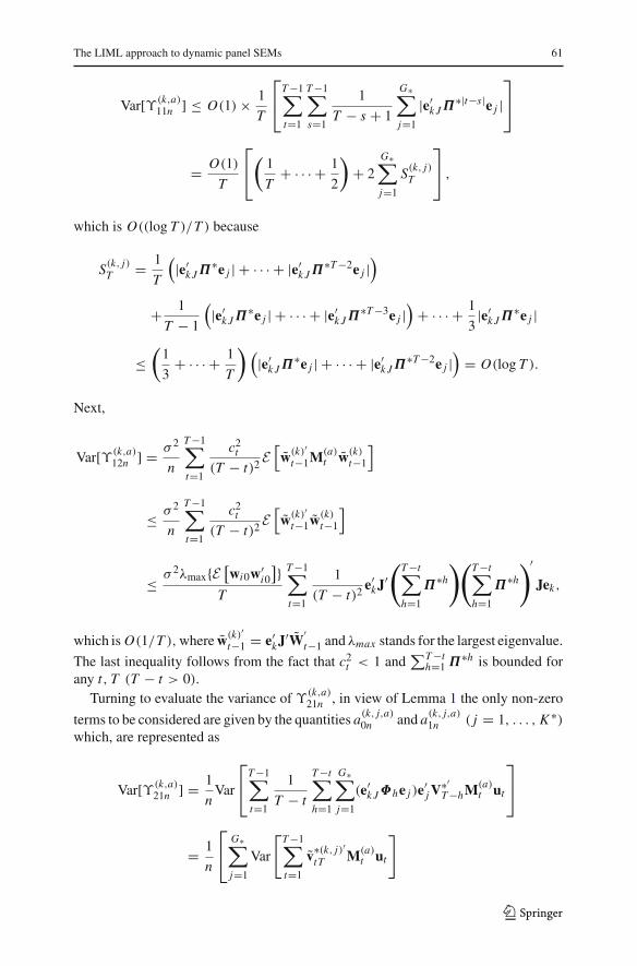
The LIML approach to dynamic panel SEMs 61
Var[ϒ(k,a)11n ] ≤ O(1)× 1
T
⎡⎣T −1∑
t=1
T −1∑s=1
1
T − s + 1
G∗∑j=1
|e′k J Π∗|t−s|e j |
⎤⎦
= O(1)
T
⎡⎣( 1
T+ · · · + 1
2
)+ 2
G∗∑j=1
S(k, j)T
⎤⎦ ,
which is O((log T )/T ) because
S(k, j)T = 1
T
(|e′
k J Π∗e j | + · · · + |e′k J Π∗T −2e j |
)
+ 1
T − 1
(|e′
k J Π∗e j | + · · · + |e′k J Π∗T −3e j |
)+ · · · + 1
3|e′
k J Π∗e j |
≤(
1
3+ · · · + 1
T
)(|e′
k J Π∗e j | + · · · + |e′k J Π∗T −2e j |
)= O(log T ).
Next,
Var[ϒ(k,a)12n ] = σ 2
n
T −1∑t=1
c2t
(T − t)2E[w(k)′
t−1M(a)t w(k)
t−1
]
≤ σ 2
n
T −1∑t=1
c2t
(T − t)2E[w(k)′
t−1w(k)t−1
]
≤ σ 2λmax{E[wi0w′
i0
]}T
T −1∑t=1
1
(T − t)2e′
kJ′(
T −t∑h=1
Π∗h
)(T −t∑h=1
Π∗h
)′Jek,
which is O(1/T ),where w(k)′t−1 = e′
kJ′W′t−1 andλmax stands for the largest eigenvalue.
The last inequality follows from the fact that c2t < 1 and
∑T −th=1 Π∗h is bounded for
any t, T (T − t > 0).Turning to evaluate the variance of ϒ(k,a)21n , in view of Lemma 1 the only non-zero
terms to be considered are given by the quantities a(k, j,a)0n and a(k, j,a)
1n ( j = 1, . . . , K ∗)which, are represented as
Var[ϒ(k,a)21n ] = 1
nVar
⎡⎣T −1∑
t=1
1
T − t
T −t∑h=1
G∗∑j=1
(e′k J Φhe j )e′
j V∗′T −hM(a)
t ut
⎤⎦
= 1
n
⎡⎣ G∗∑
j=1
Var
[T −1∑t=1
v∗(k, j)′tT M(a)
t ut
]
123
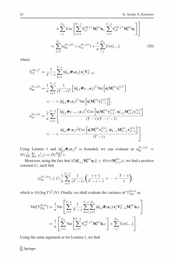
62 K. Akashi, N. Kunitomo
+G∗∑i, j
Cov
[T −1∑t=1
v∗(k,i)′tT M(a)
t ut ,
T −1∑t=1
v∗(k, j)′tT M(a)
t ut
]⎤⎦
=G∗∑j=1
(a(k, j,a)0n + a(k, j,a)
1n )+ 1
n
G∗∑i, j
Cov[., .], (50)
where
v∗(k, j)′tT = 1
T − t
T −t∑h=1
(e′
k J Φhe j)
e′j V
∗′T −h,
a(k, j,a)0n = 1
n
T −1∑t=1
1
(T − t)2
[(e′
k J ΦT −t e j)2 Var
[u′
t M(a)t v∗( j)
t
]
+ · · · + (e′k J Φ1e j
)2 Var[u′
t M(a)t v∗( j)
T −1
]],
a(k, j,a)1n = 2
n
T −2∑t=1
⎡⎣(e′
k J ΦT −t−1e j)2 Cov
[u′
t M(a)t v∗( j)
t+1 ,u′t+1M(a)
t+1v∗( j)t+1
](T − t)(T − t − 1)
+ · · · +(e′
k J Φ1e j )2Cov
[u′
t M(a)t v∗( j)
T −1,u′T −1M(a)
T −1v∗( j)T −1
](T − t)
⎤⎦ .
Using Lemma 1 and (e′k J Φhe j )
2 is bounded, we can evaluate as a(k, j,a)0n =
O( 1N T
∑t
tT −t ) = O( log T
N ).
Moreover, using the fact that |E[d′t+ j M
(a)t ut ]| ≤ O(tr(M(a)
t+ j )), we find a positiveconstant C1 such that
|a(k, j,a)1n | ≤ C1
1
n
T −2∑t=1
1
(T − t)
(t + 1
T − t − 1+ · · · + T − 1
1
),
which is O((log T )2/N ). Finally, we shall evaluate the variance of ϒ(k,a)22n as
Var[ϒ(k,a)22n ] = 1
nVar
⎡⎣T −1∑
t=1
1
T − t
T −t∑h=1
G∗∑j=1
(e′
k J Φhe j)
e′j V
∗′T −hM(a)
t utT
⎤⎦
= 1
n
⎡⎣ G∗∑
j=1
Var
[T −1∑t=1
v∗(k, j)′tT M(a)
t utT
]+
G∗∑i, j
Cov[., .]⎤⎦ .
Using the same argument as for Lemma 1, we find
123
The LIML approach to dynamic panel SEMs 63
Var[v∗(k, j)′
tT M(a)t utT
]≤ tr
(M(a)
t
) [m(1)
(v∗(k, j)
tT , utT
)+ m(3)
(v∗(k, j)
tT , utT
)]and then
m(3)(v∗(k, j)tT , utT ) = Var
[1
T − t
(e′
k J ΦT −t e jv∗( j)i t + · · · + e′
k J Φ1e jv∗( j)iT −1
)]
×Var
[1
T − t + 1(uit + · · · + uiT )
],
which is O(1/(T − t)2) because (v∗( j)i t , uit ) is independent of (v∗( j)
is , uis) for s �= t .Similarly,
m(1)(v∗(k, j)tT , utT ) = 1
(T − t)2(T − t + 1)2
× E[(
e′k J ΦT −t e jv
∗( j)i t + · · · + e′
k J Φ1e jv∗( j)iT −1
)2(uit + · · · + uiT )
2],
which is O(1/(T − t)2). Therefore, for any j , we have Var[v∗(k, j)′tT M(a)
t utT ] =O(t/(T − t)2) . From this result and the arguments as Alvarez and Arellano (2003),we conclude that Var[ϒ(k,a)22n ] = O((log T )2/N ) .Step 4: Now we evaluate the limiting distribution of the LIML estimator with thebackward-filtered instruments. We replace M(b)
t for M(a)t and define ϒ(k,b)11n , ϒ
(k,b)12n ,
ϒ(k,b)21n and ϒ(k,b)22n , accordingly. We first notice that the order of Var[ϒ(k,.)12n ] is free
with Mt , and those of ϒ(k,b)21n and ϒ(k,b)22n are reduced by the fact that tr(M(b)t ) =
O(1). For instance, Var[ϒ(k,b)12n ] = O(1/T ),Var[ϒ(k,b)21n ] = O((log T )2/(N0T )) and
Var[ϒ(k,b)22n ] = O((log T )2/(N0T )). To evaluate Var[ϒ(k,b)11n ], we prepare the nextlemma, which is a generalization of the corresponding one by Hayakawa (2006). Theproof of Lemma 2 will be provided in the online supplementary appendix.
Lemma 2 Define the N ×1 error vectors of the linear projection of Wt−1J on Z∗(b)t J,
E(b)t =[ε(1,b)t , . . . , ε
(K ,b)t
]= Wt−1J − Z∗(b)
t J[γ
∗(1,b)t , . . . , γ
∗(K ,b)t
], (51)
where Z∗(b)t = [z∗(b)
1(t−1), . . . , z∗(b)N (t−1)]′, Z∗(b)
t J = Z(b)t and γ∗(k,b)t is defined by
[γ ∗(1,b)t , . . . , γ
∗(K ,b)t ] = (b2
t limt→∞ J′E[z∗(b)i t−1z∗(b)′
i t−1]J)−1J′E[z∗(b)i t−1w
′i t−1]J;. Then,
for k = 1, . . . , K ,
E[ε(k,b)2i t ] = O
(1
t
)(52)
and
1
N0T
T −1∑t=1
J′W′t−1M(b)
t Wt−1Jp→ J′E
[wi(t−1)w′
i(t−1)
]J = J′ 0J. (53)
123
64 K. Akashi, N. Kunitomo
We turn to evaluate the order of Var[ϒ(k,b)11n ]
Var[ϒ(k,b)11n ] = 1
N0T
T −1∑t=1
T −1∑s=1
E[e′
kJ′W′t−1M(b)
t utT u′sT M(b)
s Wt−1Jek
]. (54)
For t ≥ s and k = 1, . . . , K ,
E[w(k)′
t−1M(b)t utT u′
sT M(b)s w(k)
s−1
]
= σ 2
(T − s + 1)
[E[w(k)′
t−1
(IN0 − M(b)
s
)ε(k,b)s−1
]− E
[w(k)′
t−1w(k)s−1
]
− E[ε(k,b)′t−1
(IN0 −M(b)
t
) (IN0 −M(b)
s
)ε(k,b)s−1
]+E
[ε(k,b)′t−1
(IN0 −M(b)
t
)w(k)
s−1
]],
where we use the decomposition w(k)′h−1M(b)
h = w(k)′h−1 −ε
(k,b)′h [IN0 −M(b)
h ] for h = t, s.
For the second term of the last equality, we write E[w(k)′t−1w(k)
s−1] = E[Es(w(k)′t−1)w
(k)s−1]
and then we find Var[ϒ(k,a)11n ] = O(log T/T ). Hence for the first term, we have the
same result as Step 3. As for the third term |E[ε(k,b)′t−1 (IN0 −M(b)t )(IN0 −M(b)
s )ε(k,b)s−1 ]|2
is less than
E[ε(k,b)′t−1 ε
(k,b)t−1 ε
(k,b)′s−1 ε
(k,b)s−1
]=
N0∑i=1
E[ε(k,b)2i(t−1)ε
(k,b)2i(s−1)
]+
N0∑i, j,i �= j
E[ε(k,b)2i(t−1)
] [ε(k,b)2j (s−1)
],
which O(N/(ts)) and the first equality is due to independence of random variablesε(k,b)2i(t−1). For the second inequality, we have applied Lemma 2 and the Cauchy-Schwarz
inequality as
∣∣E [ε(k,b)2i(t−1)ε(k,b)2i(s−1)
] ∣∣2 ≤(E[ε(k,b)4i(t−1)
]) (E[ε(k,b)4i(t−1)
])= O
(1
t2
)× O
(1
s2
).
Thus we can take a positive constant C2 such that
1
N0T
T −1∑s=1
2T −1∑t≥s
σ 2
T − s + 1
∣∣E [ε(k,b)′t−1
(IN0 − M(b)
t
) (IN0 − M(b)
s
)ε(k,b)s−1
] ∣∣
≤ C2N0
N0T
T −1∑s=1
2T −1∑t≥s
1
T − s + 1
1√t
1√s
= O
((log T )
√T
T
).
For the fourth term of (54), we have the same order by the similar arguments. Hence,we find that Var[ϒ(k,b)11n ] = O((log T )/
√T ).
Step 5: At this step, we drive the asymptotic covariance and bias of the limitingdistribution of the LIML estimator. First, we prepare the next lemma, which is useful
123
The LIML approach to dynamic panel SEMs 65
for deriving the covariance formula for Case (a). The proof of Lemma 3 will beprovided in the online supplementary appendix.
Lemma 3 Let (μ(1)i , . . . , μ(k)i , . . . , μ
(G∗)i )′ = μi = [
IG∗ − Π∗]−1π∗
i and Mμ =[μ1, . . . ,μN
]′. Define the N × 1 error vectors of the linear projection of MμJ on
Z(a)t ,
E(a)t =[ε(1,a)t , . . . , ε
(K ,a)t
]= MμJ − Z(a)t
[γ
∗(1,a)t , . . . , γ
∗(K ,a)t
], (55)
where for k = 1, . . . , K , h = 1, . . . , t we take each K∗t × 1 coefficient vector
γ∗(k,a)t = (γ
∗(k,a)′t1 , . . . , γ
∗(k,a)′th , . . . , γ
∗(k,a)′t t )′ as γ ∗(k,a)
thl = 1/t (if l = k) and
γ∗(k,a)thl = 0, (if l �= k), and γ
∗(k,a)th = (γ
∗(k,a)th1 , . . . , γ
∗(k,a)thl , . . . , γ
∗(k,a)thK∗ )
′. Then,for k = 1, . . . , K ,
E[ε(k,a)2i t ] = O
(1
t
)(56)
and
1
N T
T −1∑t=1
J′W′t−1M(a)
t Wt−1Jp→ J′E
[wi(t−1)w′
i(t−1)
]J = J′ 0J. (57)
For the LIML estimator, we can re-write (46) as
1√n
D′T −1∑t=1
Z( f )′t−1 Nt u
( f )t + 1√
n
T −1∑t=1
(U(⊥, f )′
tO
)Nt u
( f )t
= 1√n
D′T −1∑t=1
J′W
′t−1ut + 1√
n
T −1∑t=1
(U⊥′
tO
)Nt ut + O(1)+ op(1)
= a1n + a2n + O(1)+ op(1), (say, ) (58)
where O(1) is the associated terms of the asymptotic bias to be discussed below. Thefirst equality above is due to the result of Step 2 and the second equality follows fromNt = IN − (1 + c∗)(IN − Mt ) and
Var
[1√n
T −1∑t=1
e′k J W
′t−1(IN − Mt )ut
]= E[u2
i t ]n
T −1∑t=1
E[ε(k,.)
′(IN − Mt )ε
(k,.)]
≤ σ 2
T
T −1∑t=1
E[ε(k,.)2i t
]= O(log T )
T,
123
66 K. Akashi, N. Kunitomo
where ε(k,.)i t = ε(k,a)i t (or ε(k,a)i t ), and we have used Lemmas 2 and 3. We notice
E[a1na
′1n
]= Et [u2
i t ]n
D′E[
T −1∑t=1
J′W
′t−1Wt−1J
]D −→ σ 2Φ∗. (59)
Using the i-th unit vector ei (i = 1, . . . , N ), we find
E[a1na
′2n
]=(
1
nD
′T −1∑t=1
E[J
′W
′t−1Et
[ut u
′t Nt U⊥
t
]],O
)
=⎛⎝1
nD
′T −1∑t=1
E⎡⎣J
′W
′t−1
N∑i=1
N∑j=1
ei e′iEt
[u2
i t Nt e j u⊥′j t
]⎤⎦ ,O
⎞⎠
=(
1
nD
′T −1∑t=1
E[J
′W
′t−1dt
]E[u2
i t u⊥′i t
]( 1
1 − c
),O
),
since for any i, j, Et [u⊥j t uit ] = 0 and E[W′
t−1c∗IN ] = 0. Furthermore, we use thedecomposition
E[J
′G2
a2na′2nJG2
]= 1
n
T −1∑t=1
E[U⊥′
t Nt
[σ 2IN + (ut u
′t − σ 2IN )
]Nt U⊥
t
]
and the first term converges (1/n)∑T −1
t=1 tr(N2t )σ
2E[u⊥i t u⊥′
i t ] −→ c∗σ 2E[u⊥i t u⊥′
i t ]because we have N2
t = Mt + c2∗(IN − Mt ) and
1
n
T −1∑t=1
tr(Mt )+ c2∗1
n
T −1∑t=2
tr(IN − Mt ) = rn
n+ qn
nc2∗ −→ c∗.
Then for any constant vector h, we write the second term as
h′ 1
n
T −1∑t=1
E[U⊥′
t Nt (ut u′t − σ 2IN )Nt U⊥
t
]h
= 1
n
T −1∑t=2
N∑j=1
E[(e
′j Nt e j )
2Et
[(u2
i t − σ 2)(u⊥′i t h)2
]].
Using the similar calculations as E[a1na′2n]. Then under the assumptions we
made, we need to evaluate the convergence of [1/(N T )]∑T −1t=1 d(·)
′t W
′t−1 and
[1/(N T )]∑T −1t=1 d(·)
′t d(·)t . In each case, d(·)ti are bounded and (1/T )
∑T −1t=2 wti con-
verges to zero in probability. Further in the case of (a) maxi dit converges to zero inprobability as N → ∞. Thus, the effects of third-order terms are negligible in the
123
The LIML approach to dynamic panel SEMs 67
case of (a), while the effects of third-order terms may not be negligible in the case of(b) since N can be fixed. In both cases, we have the effects of fourth-order terms inthe general case (see Condition (IV) of Anderson et al. 2010).
Next, we evaluate the asymptotic bias of LIML estimator. We notice E[ϒ(g,a)4n ] =E[ϒ(g,b)4n ] = 0 in (47) using the fact that for any i, j, s, t, Et [u⊥
i t u js] = 0. Then in the
case of Mt = M(a)t , we evaluate the asymptotic bias as
b(a)c = Φ∗−1D′ limN ,T →∞
1√N T
T −1∑t=1
E[
Z( f )′t−1
(1
1 − ca
)(M(a)
t − caIN
)u( f )
t
]. (60)
For the term∑T −1
t=1 E[Z( f )′t−1 u( f )
t ] = −(N/T )J′E[W′
i(−1)ιT ι′T ui ], we have
E[W′
i(−1)ιT ι′T ui
]=
T −1∑h=1
T −1−h∑j=0
Π∗ jE[v∗i t uit ]
= T (IG∗ − Π∗)−1E[v∗i t uit ]
−(IG∗ −Π∗)−1[IG∗ +Π∗(IG∗ −Π∗)−1(IG∗ −Π∗T −1)]E[v∗i t uit ].
For the term∑T −1
t=1 E[Z( f )′t−1 M(a)
t u( f )t ] = −∑T −1
t=1 J′E[ct V
′tT M(a)
t u( f )t ], we can eval-
uate as
E[ct V
′tT M(a)
t u( f )t
]
= K∗t
T − t + 1
[ΦT −tE[v∗
i t uit ] − 1
T − t(ΦT −t−1 + · · · + Φ1)E[v∗
i t uit ]]
= K∗t
T − t + 1(IG∗ − Π∗)−1
[(IG∗ − Π∗T −t )− IG∗
+(
1
T − t
)[IG∗ + Π∗(IG∗ − Π∗)−1(IG∗ − Π∗T −t−1)]
]E[v∗
i t uit ] (61)
and then
T −1∑t=1
E[Z( f )′
t−1 M(a)t u( f )
t
]= −K∗(IG∗ − Π∗)−2 [(T − 1)(IG∗ − Π∗)+ O(log T )
]
×E[v∗i t uit ].
123
68 K. Akashi, N. Kunitomo
Therefore, we obtain
b(a)c = − limN ,T →∞
(K∗
1 − ca
T√N T
− ca
1 − ca
N√N T
)Φ∗−1D′J′
(IG∗ −Π∗)−1E[v∗i t uit ]
= − K∗√
limn→∞(T/N )
2 − K∗ limn→∞(T/N )Φ∗−1D′J′
(IG∗ − Π∗)−1E[v∗i t uit ]. (62)
Similarly, we consider the case of Mt = M(b)t and
T −1∑t=1
E[Z( f )′t−1 M(b)
t u( f )t ] = −K J
′(IG∗ − Π∗)−2
[(IG∗ − Π∗)− (1/T )(IG∗ − Π∗T )
]
×E[v∗i t uit ].
Then, regardless of whether N0 → ∞ or fixed, the asymptotic bias becomes
b(b)c = − limT →∞
(K
1 − cb
1√N0T
− cb
1 − cb
N0√N0T
)Φ∗−1D′J′
(IG∗ − Π∗)−1
×E[v∗i t uit ] = 0.
Step 6: We now turn to consider the asymptotic covariance matrix and the bias of theGMM estimator. The necessary arguments are basically the same as those in Step 3for the LIML estimator. If c = 0, the normalized GMM estimator are asymptoticallyequivalent to
√n(θG M − θ) = Φ∗−1
[1√n
D′T −1∑t=1
J′W
′t−1ut + 1√
n
T −1∑t=1
(J′∗G2
V′t
O
)Mt ut
]+op(1),
(63)
and J′∗G2= [0,IG2 ]. For any constant vector h we write hG = JGh, and by Lemma 1
Var
[1√n
T −1∑t=1
h′GV′
t Mt ut
]= 1
n
T −1∑t=1
Var[h′GV′
t Mt ut ] = O(c). (64)
Thus in each case, Mt = M(a)t or M(b)
t , the asymptotic variance–covariance matrixbecomes Φ∗−1(σ 2Φ∗)Φ∗−1 =σ 2Φ∗−1. Also under the condition
∑T −1t=1 tr(Mt )/(
√n)
is bounded, the asymptotic bias becomes
b(.)0 = limN ,T →∞
[1√n
T −1∑t=1
tr(Mt )
]Φ∗−1
(J′∗G2
E[vi t uit ]0
). (65)
123
The LIML approach to dynamic panel SEMs 69
Step 7: Finally, we consider the asymptotic normality of the LIML estimator (theasymptotic normality of the GMM estimator can be proven as the special case ofα2t = 0 below). Define the (G2 + K1)× 1 martingale difference sequence by
αt = α1t + α2t = 1√N
[D′J′
N∑i=1
wi(t−1)ut +(
U⊥′t
O
)Nt ut
](say, ) (66)
and then a1n + a2n = (1/√
T )∑T −1
t=1 (α1t + α2t ).
In the present situation, we have the conditions (i) (1/n)∑T −1
t=1 W′t−1(Wt−1, ιN )
p→( 0, 0), and (i) the same evaluations as used for the asymptotic covariance evaluation,for any constant vector h and any N (because uit is uncorrelated with Ft−1 and Ft−1is the σ−field generated the random variables given at t − 1), we have
1
T
T −1∑t=1
E [h′αtα′t h|Ft−1
] −→ plimT →∞1
T
T −1∑t=1
E [h′αtα′t h]
(67)
and for some constant �′ and any t, N , E[[h′(α1t + α2t )]4] < �′ . It is becauseE[[h′α1t ]4] < ∞ and E[[(c∗/
√N )t′(U⊥′
(IN − Mt )ut )]4] < ∞ using the similararguments in the next Lemma 4 below. Then the Lyapounov conditions for the centrallimit theorem hold for both cases when Mt = M(a)
t and M(b)t .
Lemma 4 For any G2 ×1 constant vector h and any t, N, there is a positive constant� such that
E[[(
1√N
)h′U⊥′
t Mt ut
]4]< �. (68)
The proof of Lemma 4 will be provided in the online supplementary appendix.
7 Appendix: Some figures
In figures, the distribution functions of estimators are shown with the standard nor-malization (the case of c = 0) and the large-K2 normalization (the case of c > 0).The limiting distributions for LIML in the large-K asymptotics are N2(0, I2) and itsmarginal distributions are N (0, 1), which are denoted as “o”. For the sake of compar-isons, the distribution of GMM are normalized in the same way and our settings aresimilar to those in Anderson et al. (2005, 2011) and Akashi and Kunitomo (2012).
See Figs. 1, 2, 3, 4, 5 and 6.
123
70 K. Akashi, N. Kunitomo
−5 −4 −3 −2 −1 0 1 2 3 4 5
0.1
0.2
0.3
0.4
0.5
0.6
0.7
0.8
0.9
1.0LIML(b) large−nGMM(b) large−nN(0,1)
LIML(b) large−KGMM(b) bias correct
Fig. 1 β2 : N = 100, T = 50, cb = 4100 , (ω11, ω12) = (1.0, 0.3)
−5 −4 −3 −2 −1 0 1 2 3 4 5
0.1
0.2
0.3
0.4
0.5
0.6
0.7
0.8
0.9
1.0LIML(b) large−nGMM(b) large−nN(0,1)
LIML(b) large−KGMM(b) bias correct
Fig. 2 γ11 : N = 100, T = 50, cb = 4100 , (ω11, ω12) = (1.0, 0.3)
123
The LIML approach to dynamic panel SEMs 71
−5 −4 −3 −2 −1 0 1 2 3 4 5
0.1
0.2
0.3
0.4
0.5
0.6
0.7
0.8
0.9
1.0LIML(b) large−nGMM(b) large−nN(0,1)
LIML(b) large−KGMM(b) bias correct
Fig. 3 β2 : N = 100, T = 50, cb = 4100 , (ω11, ω12) = (1.5, 1.0)
−5 −4 −3 −2 −1 0 1 2 3 4 5
0.1
0.2
0.3
0.4
0.5
0.6
0.7
0.8
0.9
1.0LIML(b) large−nGMM(b) large−nN(0,1)
LIML(b) large−KGMM(b) bias correct
Fig. 4 γ11 : N = 100, T = 50, cb = 4100 , (ω11, ω12) = (1.5, 1.0)
123
72 K. Akashi, N. Kunitomo
−5 −4 −3 −2 −1 0 1 2 3 4 5
0.1
0.2
0.3
0.4
0.5
0.6
0.7
0.8
0.9
1.0LIML(a) large−n
GMM(a) large−n
LIML(a) large−K
N(0,1)
Fig. 5 β2 : N = 100, T = 25, ca = 32
25100 , (ω11, ω12) = (1.0, 0.3)
−5 −4 −3 −2 −1 0 1 2 3 4 5
0.1
0.2
0.3
0.4
0.5
0.6
0.7
0.8
0.9
1.0LIML(a) large−nGMM(a) large−nN(0,1)
LIML(a) large−KGMM(a) bias correct
Fig. 6 γ11 : N = 100, T = 25, ca = 32
25100 , (ω11, ω12) = (1.0, 0.3)
123
The LIML approach to dynamic panel SEMs 73
Acknowledgments We thank the editor and two referees of this journal for helpful comments to theprevious version. The earlier versions of this paper were presented at the 2006 Japan Statistical Society(JSS) meeting, the 62nd European Meeting of the Econometric Society, and the 2010 Econometric SocietyWorld Congress (2010, Shanghai) under the title “The Conditional Limited Information Maximum Likeli-hood Approach to Panel Dynamic Structural Equations”. We also thank T.W. Anderson, Y. Matsushita, K.Hayakawa, R. Okui, K. Hitomi and Y. Nishiyama for comments to the earlier versions.
References
Akashi, K. (2008). t-test in dynamic panel structural equations (unpublished manuscript).Akashi, K., Kunitomo, N. (2012). Some properties of the LIML estimator in a dynamic panel structural
equation. Journal of Econometrics, 166, 167–183.Alonso-Borrego, C., Arellano, M. (1999). Symmetrically normalized instrumental-variable estimation using
panel data. Journal of Business and Economic Statistics, 17, 36–49.Alvarez, J., Arellano, M. (2003). The time series and cross section asymptotics of dynamic panel data
estimators. Econometrica, 71, 1121–1159.Anderson, T. W., Hsiao, C. (1981). Estimation of dynamic models with error components. Journal of the
American Statistical Association, 76, 598–606.Anderson, T. W., Hsiao, C. (1982). Formulation and estimation of dynamic models with panel data. Journal
of Econometrics, 18, 47–82.Anderson, T. W., Rubin, H. (1949). Estimation of the parameters of a single equation in a complete system
of stochastic equations. Annals of Mathematical Statistics, 20, 46–63.Anderson, T. W., Rubin, H. (1950). The asymptotic properties of estimates of the parameters of a single
equation in a complete system of stochastic equation. Annals of Mathematical Statistics, 21, 570–582.Anderson T.W., et al. (2005). A new light from old wisdoms: alternative estimation methods of simultaneous
equations with possibly many instruments, Discussion Paper CIRJE-F-321. Tokyo: Graduate School ofEconomics, University of Tokyo.
Anderson, T.W., et al. (2010). On the asymptotic optimality of the LIML estimator with possibly manyinstruments. Journal of Econometrics, 157, 191–204.
Anderson, T.W., et al. (2011). On finite sample properties of alternative estimators of coefficients in astructural equation with many instruments. Journal of Econometrics, 165, 58–69.
Arellano, M. (2003). Panel Data Econometrics. New York: Oxford University Press.Arellano, M., Bover, O. (1995). Another look at the instrumental variable estimation of error-components
models. Journal of Econometrics, 68, 29–51.Baltagi, B.H. (2005). Econometric Analysis of Panel Data (3rd ed.). New York: Wiley, Hoboken.Blundell, R., Bond, S. (2000). GMM estimation with persistent panel data : an application to production
function. Econometric Review, 19–3, 321–340.Hahn, J., Kuersteiner, G. (2002). Asymptotically unbiased inference for a dynamic panel model with fixed
effects when both n and T are large. Econometrica, 70, 1639–1657.Hayakawa, K. (2006). Efficient GMM estimation of dynamic panel data models where large heterogeneity
may be present. Tokyo: Hi-Stat Discussion Paper No.130, Hitotsubashi University.Hayakawa, K. (2009). A simple efficient instrumental variable estimator in panel AR(p) models. Econo-
metric Theory, 25, 873–890.Holtz-Eakin, D., et al. (1988). Estimating vector autoregressions with panel data. Econometrica, 56, 1371–
1395.Hsiao, C. (2003). Analysis of Panel Data (2nd ed.). Cambridge: Cambridge University Press.Kunitomo, N. (1980). Asymptotic expansions of distributions of estimators in a linear functional relationship
and simultaneous equations. Journal of the American Statistical Association, 75, 693–700.Kunitomo, N. (2012). An optimal modification of the LIML estimation for many instruments and persistent
heteroscedasiticity. Annals of Institute of Statistical Mathematics, 64, 881–910.Kunitomo, N., Akashi, K. (2010). An asymptotically optimal modification of the panel LIML estimation for
individual heteroscedasticity. Tokyo: Discussion paper CIRJE-F-780, Graduate School of Economics,University of Tokyo. http://www.cirje.e.u-tokyo.ac.jp/research/dp
123