Munich Personal RePEc Archive

The Logic of Value and the Value of

Logic

Kakarot-Handtke, Egmont

University of Stuttgart, Institute of Economics and Law

22 February 2014

Online at https://mpra.ub.uni-muenchen.de/53877/

MPRA Paper No. 53877, posted 24 Feb 2014 16:47 UTC

The Logic of Value and the Value of Logic

Egmont Kakarot-Handtke*

Abstract

Jevons composed his value theory of nonenties. These creatures are elusive.

Subsequent formal refinements did not eliminate the fundamental flaw but

made it only harder to detect. A vacuous formal structure is one that cannot

be interpreted in some domain. For want of any correspondence in the mone-

tary economy, Jevons’s approach could not produce viable results. Roughly

speaking, Jevons made value dependent on subjective factors. This paper

gives a rigorous formal proof that value is determined by objective conditions.

Within the structural-axiomatic framework there is no formal spare room for

the major behavioral nonentities utility, optimization, rational expectations,

and equilibrium.

JEL B59, D01, D61

Keywords new framework of concepts; structure-centric; axiom set; entity; nonen-

tity; principles; exchange value; allocation; Jevonian interlude

*Affiliation: University of Stuttgart, Institute of Economics and Law, Keplerstrasse 17, 70174

Stuttgart, Germany. Correspondence address: AXEC-Project, Egmont Kakarot-Handtke, Hohen-

zollernstraße 11, 80801 München, Germany, e-mail: handtke@axec.de

1

1 Entities and nonentities

Repeated reflection and inquiry have led me to the somewhat novel

opinion, that value depends entirely on utility. (Jevons, 1911, p. 1),

original emphasis

When a person sparks a surprising amount of assent, sympathy, or enthusiasm the

need for a characterization is felt and we say that the person has charisma. The word

functions like the X in an equation. Up to this point not much has happened. We

use one word as a shorthand for a complex and ill-understood social phenomenon.

The trouble begins with inversion, that is, when the placeholder word is used in

an explanation. Then it signifies an identifiable active entity, for example in the

statement: Y won the election because he/she has charisma. Unwittingly one has

slithered into a logical circle. In his methodological writings J. S. Mill criticized

this habitual reification:

Mankind in all ages have had a strong propensity to conclude that

wherever there is a name, there must be a distinguishable separate

entity corresponding to the name; . . . (Mill, 2006b, p. 756)

As long as we cannot identify charisma directly or indirectly in some objective form

any explanation that employs the word is vacuous and not acceptable, at least for

the present, according to scientific standards. Day-to-day communication is mainly

made up of socially accepted reifications. A nonentity’s reality content consists

exclusively in the degree of popular consent. As a matter of fact, most people are

talking most of the time about nonentities and all sounds sensible.

When economists are criticized for employing unrealistic, weird, or empty concepts

the answer is usually (a) physicists do the same, (b) it is an elegant abstraction, (c) it

is only to be understood ‘as if’, (d) it is not decisive for the argument, (e) there is no

alternative. All this sounds good and right but it begs the question. The point of the

criticism is usually that a specific unrealism, the auctioneer for instance, cannot be

justified by (a) to (e) or, for that matter, by any stretch of the imagination.

In general, it is indeed perfectly legitimate to introduce unrealistic or weird concepts

in a conjecture. Newton’s occult force of gravity is the paradigmatic case.

It does not matter that moos and goos cannot appear in the guess. You

can have as much junk in the guess as you like, provided that the

consequences can be compared with experiment. (Feynman, 1992, p.

164)

From this follows, as a matter of course, that not all unrealistic or weird concepts are

acceptable. Those that have no testable implication are not. Hence, they have to go

2

out of the window as fast as possible. To recall, physicists have an impressive track

record for both creating and eliminating scores of nonentities. Paradigmatic cases

are epicycles, phlogiston, ether, absolute space and the perpetual motion machine.

It is important, though, to be aware that there is no convenient criterion available

for a hard and fast distinction between an entity and a nonentity. This occasionally

long lasting indecision provides the ecological niche for nonentities.

There are two kinds of unrealism or weirdness: justified and unjustified. Newton

underpinned his occult force with a neat formula. The calculations that were carried

out with it proved to be quite accurately in correspondence with facts. Nothing

roughly comparable ever happened with, for example, utility. Jevons offered his

fellow economists this nonentity as an explanation of economic phenomena and

the great majority eventually adopted it, not realizing that, on closer inspection, it

cannot, as a matter of principle, explain anything.

Newton called assumptions that lack an objective referent hypotheses. And he was

quite explicit that employing nonentities has more to do with fiction than science.

Those who take the foundations of their speculations from hypotheses,

even if they then proceed most rigorously according to mechanical laws,

are merely putting together a romance, elegant perhaps and charming,

but nevertheless a romance. (Roger Cotes, Preface to the second edition

of Newton’s Principia, Newton, 1999, p. 386)

The romance of standard economics, rigorous and elegant as it is, has been based

on four behavioral nonentities: utility, optimization, rational expectation, and equi-

librium. The present paper is concerned in greater detail with the role of utility in

the explanation of value.

2 Words don’t matter – do they?

One must be able to say at all times – instead of points, straight lines,

and planes – tables, chairs, and beer mugs. (Hilbert, 1935, p. 403)

Formally, a theory consists of premises and conclusions or axioms and theorems;

and, hopefully, it tells us something important about reality that we hitherto did

not know. In mathematics, we have solely axioms and theorems. Here, the key

point of axiomatization is that basic concepts are not defined with reference to real

world objects and relations, but implicitly and uno actu by laying down the set of

axioms. Thus, the axioms can have an arbitrary number of real world interpretations.

Or, vice versa, entirely different and seemingly unrelated real world phenomena

may be expressible by the same axiomatic structure. For the mathematicians

the formal properties of an axiom set and its logical implications are of primary

3

interest; they can deal with them without ever taking notice of the possible real

world interpretations. Hence the question of the realism or unrealism of basic

concepts does not arise at all. The axioms create a self-contained formal world

that surprisingly often, but by no means always, finds a correspondence in the real

world.

From the axiomatic point of view, mathematics appears thus as a store-

house of abstract forms – the mathematical structures; and it so happens

– without our knowing why – that certain aspects of empirical reality

fit themselves into these forms, as if through a kind of preadaptation.

(Bourbaki, 2005, p. 1276)

Debreu took advantage of this dichotomy. His proof of the existence of a price

vector that satisfies the conditions of market clearing, budget balancing and Pareto

optimality does, in the strict sense, in no way deal with the economy but exclusively

with a clearly defined mathematical object that has no meaning beyond itself. Strictly

speaking, it would make no difference if price, market, and budget were replaced by

table, chair and beer mug. Realism or unrealism is not an issue at the formal base

line.

Allegiance to rigor dictates the axiomatic form of the analysis where

the theory, in the strict sense, is logically entirely disconnected from its

interpretations. (Debreu, 1959, p. x)

This is fine as long as the discussion is kept within the mathematical sphere. Prob-

lems arise when it comes to a real world interpretation. Without interpretation,

Debreu’s mathematical object has nothing at all to do with economics or anything

else outside mathematics.

Formal axiomatic systems must be interpreted in some domain . . . to

become an empirical science. (Boylan and O’Gorman, 1995, p. 198)

Lacking an interpretation that establishes some convincing correspondences with

real world phenomena general equilibrium is a nonentity. This, clearly, is not an

argument against axiomatization.

My opinion continues to be that axiomatics, like every other tool of

science, is no better than its user, and not all users are skilled. (Clower,

1995, p. 308)

The standard axiomatic approach has to be rejected because it does not afford a valid

interpretation in terms of the monetary economy we happen to live in; its formalism

belongs to the ‘whole crop of monster-structures, entirely without application’ (cf.

Bourbaki, 2005, p. 1275, fn. 9). The accustomed approach is beyond repair, yet:

4

There is another alternative: to formulate a completely new research

program and conceptual approach. As we have seen, this is often

spoken of, but there is still no indication of what it might mean. (Ingrao

and Israel, 1990, p. 362)

The conceptual consequence of the present paper is to discard the familiar subjective-

behavioral axioms and to take objective-structural axioms as the formal point of

departure.

In the following, Section 3 first provides the new formal foundations with the set

of four structural axioms. These represent the evolving consumption economy as

the most elementary economic configuration. The structural axiom set excludes

nonentities. In Section 4 the properties of the market clearing price for a reproducible

monetary economy are determined. In Section 5 the economy is differentiated. This

raises the question of how the labor input is allocated. It is shown that the zero profit

condition determines the exchange value and that the breakup of the expenditure

ratios determines the allocation. With the help of the obtained results it is then

possible to exactly localize, in Section 6, the logical black holes in Jevons’s approach.

Section 7 concludes.

3 Principles

When the premises are certain, true, and primary, and the conclusion

formally follows from them, this is demonstration, and produces sci-

entific knowledge of a thing. (Resume of Aristotle’s Analytica Priora,

from Wikipedia Posterior Analytics, 2014 Feb)

The formal foundations of theoretical economics must be nonbehavioral and epit-

omize the interdependence of the real and nominal variables that constitutes the

monetary economy.

3.1 Axioms

The first three structural axioms relate to income, production, and expenditure

in a period of arbitrary length. The period length is conveniently assumed to be

the calendar year. Simplicity demands that we have for the beginning one world

economy, one firm, and one product. Axiomatization is about ascertaining the

minimum number of premises.

Total income of the household sector Y in period t is the sum of wage income, i.e.

the product of wage rate W and working hours L, and distributed profit, i.e. the

product of dividend D and the number of shares N. Nothing is implied at this stage

about who owns the shares.

5

Y =WL+DN |t (1)

Output of the business sector O is the product of productivity R and working hours.

O = RL |t (2)

The productivity R depends on the underlying production process. The 2nd axiom

should therefore not be misinterpreted as a linear production function.

Consumption expenditures C of the household sector is the product of price P and

quantity bought X .

C = PX |t (3)

The axioms represent the pure consumption economy, that is, no investment, no

foreign trade, and no government.

The period values of the axiomatic variables are formally connected by the familiar

growth equation, which is added as the 4th axiom.

Zt = Zt−1

(

1+...Zt

)

with Z←W, L, D, N, R, P, X , . . .

(4)

The path of the representative variable Zt is then determined by the initial value Z0

and the rates of change...Z t for each period.

For a start it is assumed that the elementary axiomatic variables vary at random.

This produces an evolving economy. The respective probability distributions of the

change rates are given in general form by:

Pr(lW ≤

...W ≤ uW

)Pr (lR ≤

...R ≤ uR)

Pr (lL ≤...L ≤ uL) Pr (lP ≤

...P ≤ uP)

Pr (lD ≤...D ≤ uD) Pr (lX ≤

...X ≤ uX)

Pr (lN ≤...N ≤ uN) |t.

(5)

The four axioms, including (5), constitute a simulation. The simulation replaces

the inoperative set of equations as analytical tool. There is no need at this early

stage to discus the merits and demerits of different probability distributions, which,

by the way, need not be fix over time. It is, of course, also possible to switch to

a completely deterministic rate of change for any variable and any period. The

structural formalism does not require a preliminary decision between determinism

and indeterminism. If, for instance, the upper (u) and lower (l) bounds of the

respective intervals are symmetrical around zero this produces a drifting or stationary

economy as a limiting case of the growing economy.

6

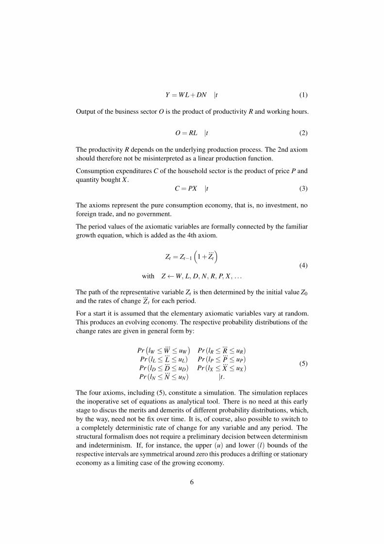
The economic content of the four axioms is plain. One point to mention is that total

income in (1) is the sum of wage income and distributed profit and not of wage

income and profit. This distinction makes all the difference between good or bad

economics (see 2013a).

3.2 Definitions

Income categories

Definitions are supplemented by connecting variables on the right-hand side of

the identity sign that have already been introduced by the axioms. With (6) wage

income YW and distributed profit YD is defined:

YW ≡WL YD ≡ DN |t. (6)

Definitions add no new content to the set of axioms but determine the logical context

of concepts. New variables are introduced with new axioms.

Given the paths of the elementary variables, the development of the composed

variables is also determined. From the random paths of employment L and wage

rate W follows the path of wage income YW . Likewise follows from the paths of

dividend D and number of shares N the path of distributed profit YD. From the 1st

axiom then follows the random path of total income Y.

Ratios

We define the sales ratio as:

ρX ≡X

O|t. (7)

A sales ratio ρX = 1 indicates that the quantity bought/sold X and the quantity

produced O are equal or, in other words, that the product market is cleared.

We define the expenditure ratio as:

ρE ≡C

Y|t. (8)

An expenditure ratio ρE = 1 indicates that consumption expenditures C are equal to

total income Y , in other words, that the household sector’s budget is balanced.

7

Monetary profit

Total profit consists of monetary and nonmonetary profit. Here we are at first

concerned with monetary profit. Nonmonetary profit is treated at length in (2011).

The business sector’s monetary profit/loss in period t is defined with (9) as the

difference between the sales revenues – for the economy as a whole identical with

consumption expenditure C – and costs – here identical with wage income YW :

Qm ≡C−YW |t. (9)

Because of (3) and (6) this is identical with:

Qm ≡ PX−WL |t. (10)

This form is well-known from the theory of the firm.

The Profit Law

From (9) and (1) follows:

Qm ≡C−Y +YD |t (11)

or, using the definitions (7) and (8),

Qm ≡

(

ρE −1

1+ρD

)

Y

with ρD ≡YD

YW

|t.

(12)

The four equations (9) to (12) are formally equivalent and show profit under different

perspectives. The Profit Law (12) tells us that total monetary profit is zero if ρE = 1

and ρD = 0. Profit or loss for the business sector as a whole depends on the

expenditure and distributed profit ratio and nothing else (for details see 2013a).

It is important to notice that neither Jevons nor the other founding fathers of marginal-

ism developed a correct profit theory.

Nor do the modern variants add anything whatever on this score. For

Debreu profits are simply a nonissue, while Arrow and Hahn make

only passing reference to profits – and that only as a historical intro-

duction. Whatever may be the usefulness of these idealized theoretical

constructs, they cannot be said to throw any light on the profit issue;

surely, therefore, they fail to capture the essence of a capitalist market

economy. (Obrinsky, 1981, p. 495)

8

The lack of a correct profit theory alone suffices to make the standard approach unfit

for any real world application whatsoever.

Individual monetary profit

For firm 1 individually eq. (10) reads in the case of market clearing:

Qm1 ≡ P1X1−W1L1

Qm1 ≡ P1R1L1

(

1−W1

P1R1

)

if ρX1 = 1 |t.

(13)

Monetary profit of firm 1 is zero under the condition that the quotient of wage rate,

price, and productivity is unity. This holds independently of the level of employment

or the size of the firm. From the zero profit condition follows:

P1 =W1

R1

if ρX1 = 1, Qm1 = 0 |t.

(14)

The price of product 1 is, in the simplest case, equal to unit wage costs.

Relative prices

In the same way one gets the individual profits and the zero profit market clearing

prices for all other firms. With this, the structure of relative prices is determined for

the most elementary case.

P1

P2

=

W1

R1

W2

R2

=R2

R1

if W1 =W2, ρX1 = 1, ρX2 = 1, Qm1 = 0, Qm2 = 0 |t.

(15)

Under the zero profit condition, relative prices stand in the same relation as unit

wage costs. With equal wage rates, relative prices stand in inverse relation to

productivities.

This limiting case is the structural-axiomatic counterpart to Walras’s zero profit

general equilibrium. In the case of a non-zero profit economy the derivation of the

market clearing price vector is a bit more involved.

9

From relative prices in (15) we advance to the classical term value:

The word Value, when used without adjunct, always means, in political

economy, value in exchange; or as it has been called by Adam Smith

and his successors, exchangeable value, . . . (Mill, 2006a, p. 457)

If P1 is double P2 then half a unit of X1 exchanges for one unit of X2. Eq. (15) states

that the exchange value is, under the condition of zero profit and equal wage rates

in the two lines of production, equal to the inverse of the productivities. Value is

objectively determined by the production conditions. There is no formal room left

for subjective-behavioral notions like utility. The zero profit condition is sufficient

to exclude utility as an explanation of value.

Retained profit

Once profit has come into existence for the first time (that is: logically – a historical

account is an entirely different matter) the business sector has the option to distribute

or to retain it. This in turn has an effect on profit. This effect is captured by (11) but

it is invisible in (9). Both equations, though, are formally equivalent.

Retained profit Qre is defined for the business sector as a whole as the difference

between profit and distributed profit in period t:

Qre ≡ Qm−YD ⇒ Qre ≡C−Y |t. (16)

Retained profit is, due to (11), equal to the difference of consumption expenditures

and total income.

Monetary saving

The household sector’s monetary saving is given as the difference of income and

consumption expenditures (for nonmonetary saving see 2011):

Sm ≡ Y −C |t. (17)

In combination with (16) follows:

Qre ≡−Sm |t. (18)

Monetary saving and retained profit always move in opposite directions. This is

the Special Complementarity. It says that the complementary notion to saving is

negative retained profit; positive retained profit is the complementary of dissaving.

10

There is no such thing as an equality of saving and investment in the consumption

economy, nor, for that matter, in the investment economy (for details see 2013b).

If distributed profit is zero then follows as a corollary of (18):

Qm =−Sm

if YD = 0

|t. (19)

Profit is zero in the limiting case of zero distributed profit and zero saving. Otherwise

profit is equal to dissaving, loss is equal to saving in a given period. To focus the

analysis, distributed profit and saving is set to zero in the following.

3.3 Nonentities excluded

Equilibrium in whatever definition is not taken into the premises. Methodologically,

this would amount to a petitio principii (cf. Mill, 2006b, pp. 819-827). Not admitted

are, in addition, utility, optimization, and rational expectation. The first rule of

theory building says: never put a behavioral assumption into the premises, or, as

Newton famously said: hypotheses non fingo.

4 The market clearing price

But in political economy the greatest errors arise from overlooking the

most obvious truths. (Mill, 2006a, p. 458)

From (3), (7), and (8) follows the price as dependent variable:

P =ρE

ρX

W

R

(

1+YD

YW

)

|t. (20)

This is the general structural axiomatic law of supply and demand for the pure

consumption economy with one firm (for the generalization see 2014a). In brief,

the price equation states that the market clearing price, i.e. ρX = 1, is ultimately

determined by the expenditure ratio, unit wage costs, and the income distribution.

Note that the quantity of money is not among the determinants. This rules the

commonplace quantity theory out. The structural axiomatic price formula is testable

in principle.

Under the condition of market clearing and zero distributed profit follows:

11

P = ρE

W

R

if ρX = 1, YD = 0 |t.

(21)

The market clearing price depends now alone on the expenditure ratio and unit

wage costs. All changes of the wage rate, of the productivity, and of the average

expenditure ratio affect the market clearing price in the period under consideration.

We refer to this formal property as conditional price flexibility because (21) involves

no assumption about human behavior, only the purely formal condition ρX = 1.

Under the additional conditions of budget balancing follows:

P =W

R

if ρE = 1, ρX = 1, YD = 0 |t.

(22)

The market clearing price is equal to unit wage costs if the expenditure ratio is unity

and distributed profit is zero. In this elementary case, profit per unit is zero and by

consequence total profit is zero. All changes of the wage rate and the productivity

affect the market clearing price in the period under consideration.

With (22) the real wage WP

is uno actu given; it is under the enumerated conditions

invariably equal to the productivity R. The agents gets the whole product. The real

wage is determined by the production conditions and not in the labor market.

With regard to standard economics, the structural axiom set has two important

implications: (a) the market clearing price is not determined by the quantity of

money, (b) the real wage is not determined by supply-demand-equilibrium in the

labor market. In other words, seen from the structural-axiomatic standpoint the

commonplace quantity theory and the standard labor market theory are false.

It has to be emphasized that market clearing, budget balancing, and zero profit

are conditions that apply also to Walras’s original model. On this score, there is

absolutely no difference.

5 Allocation in the two-markets consumption economy

The theory thus represents the fact, that a person distributes his income

in such a way as to equalize the utility of the final increments of all

commodities consumed. (Jevons, 1911, p. 140)

We now introduce a second market and determine the allocation of total labor

input L between the two lines of production.

12

Total income (1) remains unchanged:

Y =WL+ DN︸︷︷︸

0

|t. (23)

The partitioning of labor input is given by:

L≡ L1 +L2 |t. (24)

With given productivities the respective outputs in the two lines of production follow

from (2) as:

O1 = R1L1

O2 = R2L2|t. (25)

From (3) follows for the respective consumption expenditures:

C1 = P1X1

C2 = P2X2|t. (26)

From (8) follow as corollaries:

C1 = ρE1Y

C2 = ρE2Y

if ρE1, ρE1 are taken as independent |t.

(27)

Under the condition of market clearing eqs. (27), (26) and (25) boil down to:

P1

P2

R1

R2

L1

L2

=ρE1

ρE2

if ρX1 = 1, ρX2 = 1 |t.

(28)

Relative prices are determined by the zero profit condition (15) and this gives:

L1

L2

=ρE1

ρE2

if Qm1 = 0, Qm2 = 0, W1 =W2, ρX1 = 1, ρX2 = 1 |t.

(29)

Under the enumerated conditions, the labor input is allocated in direct proportion

to the expenditure ratios. The partitioning of demand determines the allocation of

labor. This presupposes, of course, that labor can move freely between the two

13

firms. The absolute amount of labor input in firm 1, and analogous in firm 2, is

finally given by:

L1 = ρE1L

if Qm1 = 0, Qm2 = 0, W1 =W2, ρX1 = 1, ρX2 = 1

L≡ L1 +L2, ρE1 +ρE2 = 1 |t.

(30)

What remains to be done is to determine the partitioning of final demand between

the two goods. Here we arrive at the open interface to utility theory.

Eq. (28) is first rewritten as:

P1

P2

X1

X2

=ρE1

ρE2

if ρX1 = 1, ρX2 = 1 |t.

(31)

The familiar optimum condition says that the marginal rate of substitution MRS is

equal to the price ratio. This condition is met at the tangential point of the budget

line with an indifference curve (for details see 2014a, Sec. 3.3). The tangential point

provides the respective quantities X1, X2. Together with the given price relation

eq. (31) then delivers the optimal partitioning of the consumption expenditures

C1, C2 or, what amounts to the same, the optimal breakup of the expenditure ratios

ρE1, ρE2. All is fine therefore, except for the fact that the indifference curve is a

nonentity.

The marginal principle asserts, in Jevons’s language, that the ratio of marginal

utilities is equal to relative prices but it cannot tell us where the tangential point is lo-

cated. Hence there is no way to determine the quantities X1, X2 and by consequence

the distribution of expenditures between the goods. In plain words Jevons asserts, I

cannot give you the coordinates where the agents stand but it is an optimum. This

optimum, though, he has put himself into the hat.

It would be possible at any time to integrate marginal utility into the structural-

axiomatic framework in order to determine the expenditure ratios for different

products but this amounts to nothing because the marginal principle cannot tell us

what we want to know. To ask: where does an indifference curve touch the budget

line is, apart from the wording, not different from asking how many angels can

dance on the head of a pin.

Economists think of themselves as scientists, but . . . they are more like

theologians. (Nelson, 2006, p. xv)

In any case they are primarily concerned with nonentities.

14

6 Winding up the Vacuous Jevonian Interlude

Reification (also known as concretism, or the fallacy of misplaced

concreteness) is a fallacy of ambiguity, when an abstraction (abstract

belief or hypothetical construct) is treated as if it were a concrete, real

event, or physical entity. In other words, it is the error of treating as

a concrete thing something which is not concrete, but merely an idea.

(Wikipedia Reification, 2014 Feb)

6.1 Value and allocation

We have seen above, eq. (15), that the exchange value is objectively determined by

the zero profit condition and therefore has nothing at all to do with a final degree of

utility. From the systemic standpoint it is irrelevant whether the agents realize some

kind of optimum or not. It is not irrelevant, though, whether the firms break even or

not. An economy with loss making firms is not reproducible over a longer time span.

Zero profit is a minimum condition, positive overall profit is the normal case in the

real world. Jevons’s profit formula, (1911, p. 270), is demonstrably false and this,

as a matter of principle, invalidates his value theory already before the speculation

about the final degree of utility sets in. Independently of this, the subjective value

theory has to be refuted on its own terms.

Let us start with an economy where the respective productivities in period t=1 are

given by the actual production conditions and where the households have partitioned

their total consumption expenditures which in turn are equal to total income. The

conditions of market clearing, budget balancing and zero profit apply. For the sake

of illustration, let the two products be bread and water (wine would be better, of

course, but not straightforwardly lead us to the water-diamond paradox). In this case,

the exchange value of water is objectively determined by the production conditions

in both firms according to (15) (see also Arrow and Hahn, p. 14).

The quantity of water that is produced and sold depends on the partitioning of

consumption expenditures according to (29). If the expenditure ratio for water

is high relative to that for bread, the greater part of labour input is allocated to

water production. The breakup of expenditure ratios can be observed and exactly

measured for all households and all periods. There is no problem with the data. Yet,

why the expenditure ratios are what they are is unknown to any observer. To say

that the partitioning depends on preferences is neither true nor false but a pointless

reification. To assert that the partitioning is optimal is pure verbiage. An utility

function or an indifference map is a nonentity and that is that.

Now let the productivity of water production increase in period t=2. The first

round effect is this: the price goes down and the quantity goes up such that total

expenditures for water remain constant. This hyperbolic adaptation leaves the rest

of the economy undisturbed. The only thing that changes is the real consumption

15

pattern. The households’ diet is now composed of more water and an unchanged

quantity of bread. Hyperbolic adaptation, to be sure, is a convenient idealization.

The households may be happy with the new composition of consumption goods. In

this case, the adaptation process ends. If the households want to restore the previous

relation of water and bread they have to reduce the expenditures for water and to

increase the expenditures for bread. The business sector then reallocates labor input

at the going wage rate. There is no price signaling of any sort. Total income, total

consumption expenditures, and the price of water and bread are not affected by the

reallocation. The price mechanism is fully replaced by the quantity mechanism.

At the end of the adaptation process, which consists of two logical steps, the

exchange value of water is lower according to the new productivities as determined

by (15). The claim that the marginal utilities of water and bread have been equal

before the adaptation and are equal after the adaptation can neither be proved nor

disproved, it is therefore empty.

There is no need and no place for the nonentity utility and its derivatives and variants

in theoretical economics. Theoretical economics is about the systemic properties of

the economy and not about reading the thoughts of agents. There is nothing ever to

be expected from second-guessing homo oeconomicus.

6.2 Primary and secondary markets

Up to this point we have only considered perishable consumption goods. Conditions

change when we take durable goods into the picture. A car or a house is bought in

period t but consumed over a longer time span; consumption expenditures C and

valued consumption K are therefore different (for details see 2011, Sec. 4.2).

Conditions are again different when, in the limiting case, no consumption takes

place at all. Ricardo clearly recognized this and excluded “rare statues and pictures,

scarce books and coins, . . . ” from the classical value theory (1981, p. 12). Jevons

took up this remark and used it as a refutation of the labour theory of value (1911, p.

163). He did not realize that goods which are not consumed like bread and water

are not subject to his own Law of the Variation of Utility which refers explicitly

to varying quantities of food (1911, pp. 45-49). Adam Smith’s narrow-stomach

argument does not apply beyond a very small realm.

Let the two goods in the example of Section 6.1 now be diamonds and water

(yes, this combination lacks vitamins). This requires an update of the productivity

R1 and of the price P1 in (28) but nothing more. While the productivity in the

water production remains unchanged, compared to diamonds the exchange value

of one unit of water will be ‘lower’ in quantitative terms than compared to bread.

The quantities, however, have different dimensions (liter, kilogram, carat). The

respective prices of diamonds and water are definitely determined by the conditions

of market clearing, budget balancing, and zero profit.

16

Since diamonds are not consumed and do not vanish from the commodity space the

story does not end in the period of production. Beginning with the next period, the

diamonds assume the role of a store of value. At first, those agents who have bought

the diamonds in period t cannot sell them in period t+1. There is simply no market.

Since income has always been fully spent in the pure consumption economy nobody

is in the possession of the requisite stock of money. What is logically needed first,

then, is that some agents accumulate money.

Let us assume that one half of the households saves and the other half dissaves such

that saving and dissaving are equal and the household sector as a whole neither

saves nor dissaves. Thus, the overall expenditure ratio is still unity (for details see

2014b, Sec. 3). Total income is fully spent, just as in the bread-water economy. The

significant difference is that the deposits and overdrafts of the household sector at

the central bank, which stands for the banking industry as a whole, grow in lockstep.

The owners of deposits eventually become the potential buyers of diamonds.

What emerges in the process is that we have now two entirely different kinds of

markets: the primary market where the goods out of current production are sold and

the secondary market where all kinds of durables are sold.

The primary and secondary markets function according to different rules. For

the primary market the income out of current production and saving/dissaving

is relevant, for the secondary market the accumulated stock of deposits and the

possibility of credit leverage is relevant. Of course, there are interdependencies

between the two kinds of markets. They are ignored for the moment.

The crucial point is that it is positively misleading to speak of “the” market. There

are – at least – two different types of markets and to treat them equally is a gross

technical blunder. There is no such thing as “the” market. A value theory that

does not account for this elementary economic fact is vacuous. The marginalistic

approach squarely falls into this category.

What is important with regard to Jevons’s value theory is this: even if we grant,

for the sake of argument, that there is something like marginal utility it would be

only applicable to the primary market but not to the secondary market. Water as

a consumption good is not comparable to diamonds as a pure store of value. The

assertion that the low price of water corresponds to a low marginal utility and that

the high price of diamonds corresponds to a high marginal utility is unacceptable

even in Jevons’s own frame of reference. To apply the Law of the Variation of

Utility to the secondary market is simply a category mistake.

What is really paradoxical about the diamond-water paradox is that its apparent

resolution by superficially distinguishing between total and marginal utility was

accepted so long by so many economists. Fortunately, that is over now. Utility has

been definitely identified as nonentity. As Keynes aptly put it (Moggridge, 1976, p.

39): ‘a little clear thinking’ can solve ‘almost any problem.’

17

7 Conclusion

Our science has become far too much a stagnant one, in which opinions

rather than experience and reason are appealed to. (Jevons, 1911, p.

277)

The secular stagnation of the standard approach can be traced back to Jevons himself.

His approach, which has been greatly refined but never thoroughly rectified, is based

on indefensible premises.

The standard subjective-behavioral axioms are in the present paper replaced by

objective-structural axioms. The set of four structural axioms constitutes the most

elementary case of an evolving consumption economy. The formalism is absolutely

transparent, the logical implications are testable in principle.

The main results of the structural axiomatic analysis of value are:

• Neither Jevons nor the other founding fathers of marginalism developed a

correct profit theory. The lack of a correct profit theory alone suffices to make

the standard approach unfit for any real world application whatsoever.

• Exchange value is objectively determined by the production conditions and

therefore has nothing at all to do with a final degree of utility. There is no

formal room left for subjective-behavioral notions like utility. The zero profit

condition is sufficient to exclude utility as an explanation of value.

• The structural-axiomatic conditions of market clearing, budget balancing,

and zero profit apply also to Walras’s original model. On this score, there is

absolutely no difference. The difference is in the axioms.

• It would be possible at any time to integrate marginal utility into the structural-

axiomatic framework in order to determine the expenditure ratios for different

products but this amounts to nothing because the marginal principle cannot

tell us what we want to know.

• There are – at least – two different types of markets and to treat them equally

is a gross technical blunder. There is no such thing as “the” market. A value

theory that does not account for this elementary economic fact is vacuous.

The marginalistic approach squarely falls into this category.

18

References

Arrow, K. J., and Hahn, F. H. (1991). General Competive Analysis. Amsterdam,

New York, NY, etc.: North-Holland.

Bourbaki, N. (2005). The Architecture of Mathematics. In W. Ewald (Ed.), From

Kant to Hilbert. A Source Book in the Foundations of Mathematics, volume II,

pages 1265–1276. Oxford, New York, NY: Oxford University Press. (1948).

Boylan, T. A., and O’Gorman, P. F. (1995). Beyond Rhetoric and Realism in Eco-

nomics. Towards a Reformulation of Economic Methodology. London: Routledge.

Clower, R. W. (1995). Axiomatics in Economics. Southern Economic Journal,

62(2): 307–319. URL http://www.jstor.org/stable/1060684.

Debreu, G. (1959). Theory of Value. An Axiomatic Analysis of Economic Equilib-

rium. New Haven, London: Yale University Press.

Feynman, R. P. (1992). The Character of Physical Law. London: Penguin.

Hilbert, D. (1935). Gesammelte Abhandlungen, volume III. Berlin:

Julius Springer. URL http://gdz.sub.uni-goettingen.de/dms/load/img/?PPN=

PPN237834022&IDDOC=42376.

Ingrao, B., and Israel, G. (1990). The Invisible Hand. Economic Equilibrium in the

History of Science. Cambridge, MA, London: MIT Press.

Jevons, W. S. (1911). The Theory of Political Economy. London, Bombay, etc.:

Macmillan, 4th edition. URL http://www.econlib.org/library/YPDBooks/Jevons/

jvnPE.html.

Kakarot-Handtke, E. (2011). Primary and Secondary Markets. SSRN Working Paper

Series, 1917012: 1–26. URL http://ssrn.com/abstract=1917012.

Kakarot-Handtke, E. (2013a). Confused Confusers: How to Stop Thinking Like

an Economist and Start Thinking Like a Scientist. SSRN Working Paper Series,

2207598: 1–16. URL http://ssrn.com/abstract=2207598.

Kakarot-Handtke, E. (2013b). Why Post Keynesianism is Not Yet a Science.

Economic Analysis and Policy, 43(1): 97–106. URL http://www.eap-journal.com/

archive/v43_i1_06-Kakarot-Handtke.pdf.

Kakarot-Handtke, E. (2014a). Exchange in the Monetary Economy. SSRN Working

Paper Series, 2387105: 1–19. URL http://papers.ssrn.com/sol3/papers.cfm?

abstract_id=2387105.

Kakarot-Handtke, E. (2014b). Loanable Funds vs. Endogenous Money: Krugman

is Wrong, Keen is Right. SSRN Working Paper Series, 2389341: 1–17. URL

http://papers.ssrn.com/sol3/papers.cfm?abstract_id=2389341.

19

Mill, J. S. (2006a). Principles of Political Economy With Some of Their Applications

to Social Philosophy, volume 3, Books III-V of Collected Works of John Stuart

Mill. Indianapolis, IN: Liberty Fund. URL http://www.econlib.org/library/Mill/

mlP.html. (1866).

Mill, J. S. (2006b). A System of Logic Ratiocinative and Inductive. Being a Con-

nected View of the Principles of Evidence and the Methods of Scientific Investiga-

tion, volume 8 of Collected Works of John Stuart Mill. Indianapolis, IN: Liberty

Fund. (1843).

Moggridge, D. E. (1976). Keynes. London, Basingstoke: Macmillan.

Nelson, R. H. (2006). Economics as Religion: From Samuelson to Chicago and

Beyond. Pennsylvania, PA: Pennsylvania State University Press.

Newton, I. (1999). The Principia; Mathematical Principles of Natural Philosophy.

Berkley, CA, Los Angeles, CA, London: University of California Press. (1687).

Obrinsky, M. (1981). The Profit Prophets. Journal of Post Keynesian Economics,

3(4): 491–502. URL http://www.jstor.org/stable/4537615.

Ricardo, D. (1981). On the Principles of Political Economy and Taxation. The

Works and Correspondence of David Ricardo. Cambridge, New York, NY, etc.:

Cambridge University Press. (1821).

Website: http://www.axec.org, see Terms of use; © 2014 Egmont Kakarot-Handtke

20