The Long and Short (of) Quality Ladders∗

Amit Khandelwal†

Columbia Business School & NBER

First Draft: November 2006

This Version: October 2009

Abstract

Prices are typically used as proxies for countries’ export quality. I relax this strong assumption by

exploiting both price and quantity information to estimate the quality of products exported to the U.S.

Higher quality is assigned to products with higher market shares conditional on price. The estimated

qualities reveal substantial heterogeneity in product markets’ scope for quality differentiation, or their

“quality ladders.” I use this variation to explain the heterogeneous impact of low-wage competition on

U.S. manufacturing employment and output. Markets characterized by relatively shorter quality ladders

are associated with larger employment and output declines resulting from low-wage competition.

Keywords: Quality Ladders; Low Wage Competition; Quality Specialization; Product Differentiation

JEL Classification: F1, F15, F16

1 Introduction

The quality of products manufactured by countries affects many economic outcomes in international and

development economics. Past studies have consistently found that product quality influences cross-border

trade; richer countries consume and export higher quality products than developing countries.1 The ability∗I am especially grateful to my dissertation committee, Irene Brambilla, Penny Goldberg and Peter Schott, for guidance

and support. I have benefited from conversations with Steve Berry, Ray Fisman, Juan Carlos Hallak, David Hummels, Kala

Krishna, Chris Ksoll, Frank Limbrock, Alex Mcquoid, Nina Pavcnik, Siddharth Sharma, Gustavo Soares, Robert Staiger,

Catherine Thomas, Daniel Trefler, Chris Udry, Eric Verhoogen, David Weinstein, Jeffrey Weinstein, and various seminar

participants. This paper also benefited greatly from the comments of two anonymous referees and the editor. Special thanks

also to Amalavoyal Chari. All errors are my own.†Uris Hall, Room 606, 3022 Broadway, New York, NY 10027, email: ak2796@columbia.edu, website:

http://www0.gsb.columbia.edu/faculty/akhandelwal/.1The demand-side explanation, initially posited by Linder (1961), has been supported by Hallak (2006) and Verhoogen

(2008). Studies by Hummels and Klenow (2005) and Schott (2004) provide systematic evidence that richer countries export

1

of developing countries to transition from low-quality to high-quality products is therefore seen by some as a

necessary (but certainly not a sufficient) condition for export success and, ultimately, economic development.2

In addition, quality upgrading features prominently in current debates about the role of international trade

in driving wage inequality. But while this research suggests a positive association between quality upgrading

and income per capita, Verhoogen (2008) and Goldberg and Pavcnik (2007) argue that quality upgrading also

affects the variance of income through changes in the relative demand for skilled labor. Quality specialization

may therefore partly explain why inequality has risen in developing countries following trade liberalizations,

in contrast to Stolper-Samuelson predictions. Differences in the quality space may also affect how closely

countries’ products compete with one another and therefore have implications for the impact of trade on

industry employment and output (Leamer, 2006).

These studies stress the importance of understanding why product quality varies across countries and

over time, and how it is influenced by policy. The challenge faced by this literature is that product quality is

unobserved. Research in the international trade literature has attempted to deal with this problem by using

prices (or unit values) as a proxy for quality. This approach, while convenient, requires strong assumptions

since prices could reflect not just quality, but also variations in manufacturing costs. For example, in 1999,

the U.S. imported Malaysian and Portuguese women’s trousers (HS 6204624020) at unit values (inclusive

of transportation and tariff duties) of $146 and $371, respectively. If prices are assumed as perfect proxies

for quality, Malaysian trousers would possess about half the quality of Portuguese trousers. However, the

annual wage in the apparel sector for Malaysia and Portugal was $3,100 and $5,700, respectively (UNIDO,

2005). So the difference in unit values may instead be a reflection of these different factor prices. Why

would a consumer ever purchase expensive Portuguese trousers if they, in fact, possess lower quality? One

explanation is that a fraction of consumers have a preference for the horizontal attributes of Portuguese

trousers (for instance, the cut or color patterns). Indeed, U.S. consumers imported more than 82,000 dozens

of Malaysian trousers compared to only 865 dozens from Portugal. Idiosyncratic preferences for products’

horizontal attributes can therefore break the direct mapping from prices to quality that has been traditionally

assumed.

This paper estimates the quality of U.S. imports using a procedure that relaxes the strong quality-

equals-price assumption. The quality measures are derived from a nested logit demand system, based on

Berry (1994), that embeds preferences for both horizontal and vertical attributes.3 Quality is the vertical

higher quality products. Baldwin and Harrigan (2007), Hallak and Sivadasan (2009), Kugler and Verhoogen (2008) and Johnson

(2009) also document the role of product quality in influencing production and trade patterns.2Kremer (1993) provides microeconomic foundations for the quality production function and its implications for economic

development (see also Verhoogen (2008) and Kugler and Verhoogen (2008)). Endogenous growth models that highlight the

importance of product quality include Grossman and Helpman (1991). Hausmann and Rodrik (2003), Rodrik (2006) and

Hidalgo et al. (2007) highlight the importance of export quality for economic performance.3Other studies within international trade that use a nested logit structure include Goldberg (1995) and Irwin and Pavcnik

2

component of the estimated model and captures the mean valuation that U.S. consumers attach to an im-

ported product. The procedure utilizes both unit value and quantity information to infer quality and has

a straightforward intuition: conditional on price, imports with higher market shares are assigned higher

quality. Importantly, the procedure requires no special data beyond what is readily available in standard

disaggregate trade data. It is also easy to implement; here, I estimate separate demand curves for approxi-

mately hundreds of manufacturing industries. Moreover, the procedure recovers quality at the finest level of

product aggregation available (for the U.S. data, this is the ten-digit HS level).4

The inferred qualities indicate that developed countries export higher quality products relative to

developing countries. This finding is consistent with Schott (2004) who uses unit values as a proxy for

quality. However, the estimates also reveal substantial heterogeneity in product markets’ scope for quality

differentiation, or quality ladders, which I measure as the range of qualities within the product market. In

markets with a larger scope for quality differentiation, or a “long” quality ladder, unit values are relatively

more correlated with the estimated qualities. In these markets prices appear to be appropriate proxies for

quality. In contrast, prices appear to be less appropriate proxies for quality in markets with a narrow range

of estimated qualities (“short” ladder markets). This provides suggestive evidence that expensive imports in

short-ladder markets coexist with cheaper rivals due to horizontal product differentiation. That is, although

the average U.S. consumer attaches a low valuation to the expensive import, there is a fraction of consumers

who still value the product. This heterogeneity underscores the drawback in invoking the quality-equals-price

assumption, particularly for products characterized by short quality ladders.

I use this heterogeneity in ladder lengths to demonstrate that quality specialization has important

implications for the U.S. labor market. The public’s fear of globalization is often rooted in the vulnerability

or, to use Edward Leamer’s terminology, the contestability of jobs. According to Leamer, the contestable jobs

are those where “wages in Los Angeles are set in Shanghai” (Leamer (2006) p. 5). A recent study by Bernard,

Jensen, and Schott (2006) provides evidence that the probability of U.S. plant survival and employment

growth are negatively associated with an industry’s exposure to import penetration, particularly from low-

wage countries.5 However, while low-wage competition negatively affects output and employment growth,

the impact is heterogenous across industries. For instance, between 1980 and the mid-1990s, electronics

(SIC 36) experienced greater low-wage import penetration than fabricated metals (SIC 34) but experienced

(2004), although these papers do not focus on the quality of imported products.4An alternative procedure developed by Hallak and Schott (2007) relies on similar intuition to infer countries’ export quality

to the U.S., but their methodology prevents estimating quality at the finest level of disaggregation due to data limitations.5Other studies examining the negative relationships between trade and employment include Sachs and Shatz (1994), Free-

man and Katz (1991) and Revenga (1992). Bernard, Jensen, and Schott (2006) explicitly connect the relationship between

employment and trade with low-wage countries, defined as nations with less than 5 percent of U.S. per capita GDP. I use their

definition of low-wage countries in this paper (see Table 1).

3

a smaller employment decline.6

Using a simple model developed in Section 2, I demonstrate that the impact of low-wage compe-

tition on U.S. industries will vary with the industry’s quality ladder. My argument is related to a body

of research that rejects standard model predictions of factor price equalization (FPE).7 These studies show

that if countries inhabit different cones of (quality) diversification, with developing countries exporting low-

quality products, then developed countries will be insulated from wage movements in developing countries.

However, if markets vary in their scope for quality differentiation, developed countries will experience hetero-

geneity in their exposure to developing countries. In long-ladder markets, developed countries can insulate

themselves from the South by using comparative advantage factors (e.g., skill, capital and/or technology)

to specialize atop the quality ladder. In short-ladder markets, however, developed countries will be directly

exposed to Southern competition because quality upgrading is infeasible. Thus, a market’s scope for vertical

differentiation is important for understanding Leamer’s notion of contestable jobs.

I find robust support for this hypothesis by matching U.S. industry data and import competition to

quality ladders constructed from the estimated qualities. Consistent with Bernard et al. (2006), I find that

industry employment is negatively associated with import penetration, particularly from low-wage countries.

However, the empirical results confirm that import penetration has a weaker impact on employment in

industries with long quality ladders: a ten percentage point increase in low-wage penetration is associated

with a 6 percent employment decline in an industry characterized by an average quality ladder length. A

similar increase in competition in a long-ladder industry (one standard deviation above the mean) results in

only a 1.4 percent employment decline. Differential impacts on industry output are similar. Importantly, the

impact of import competition on short and long-ladder industries is similar in magnitude to the differential

impact on low and high capital-intensive industries. In other words, even after controlling for the differential

impact through traditional channels, such as capital and skill intensities (see Sachs and Shatz (1994) and

Bernard et al. (2006)), the quality ladder remains an important determinant of an industry’s vulnerability

to low-wage competition. Moreover, the heterogenous effect is not precisely captured if one simply uses

variations in unit values.

These results complement the literature studying the relationship between quality specialization and

labor markets. But while existing studies focus predominantly on developing countries (see Goldberg and

Pavcnik (2007), Verhoogen (2008), Kaplan and Verhoogen (2005)), the evidence here suggests that quality

specialization is also important for developed countries. Quality ladders may therefore help identify those

markets that are likely to be contested by competition from low-wage countries.6One potential explanation is differences in capital intensity, but in 1980, electronics was less capital intensive than fabricated

metals. Indeed, this paper offers evidence that capital intensity only partly explains the heterogeneity in U.S. employment

outcomes due to import competition.7For instance, see Leamer (1987) and Schott (2003).

4

The remainder of the paper is organized as follows. Section 2 offers a simple model to illustrate that

exposure to low-wage competition is greater in markets with short quality ladders. In Section 3, I discuss

the approach used to infer quality from trade data. The data and quality estimation results are presented in

Section 4. Section 5 applies the quality estimates to test the implications of quality specialization for U.S.

employment. I conclude in Section 6.

2 A Model of Contestable Jobs

This section develops a simple model that delivers two comparative static results. First, the impact of foreign

competition on domestic market shares is larger from low-wage countries. Second, the impact will depend on

the market’s quality ladder length. I then use the empirical quality measures derived in Section 3 to assess

the predictions of the model.

The model is partial equilibrium and analyzes firms in two regions, North (N) and South (S), where

the Southern firms freely export to the North. The wages in each country are determined by an outside sector

and are therefore treated as exogenous: wN > wS . Each region has J homogenous firms that compete by

manufacturing horizontally and vertically distinct varieties. Following Krugman (1980) and Melitz (2003),

horizontal differentiation is costless, so in equilibrium, all firms produce horizontally distinct varieties. But as

in Flam and Helpman (1987), vertical (e.g., quality) differentiation depends on a Ricardian-type comparative

advantage given by region c’s technology, Zc. I assume that Northern firms have access to better technology

than the South: ZN > ZS . Firm j uses this technology to manufacture a variety subject to a marginal cost

function that is increasing with quality (λj): wc + λ2j

2Zc, for c ∈ {N,S}.8

The consumers who live in the North have discrete choice preferences. Consumer n observes the

domestic and Southern varieties and chooses the variety j that provides her with the highest indirect utility:

Vnj = θλj − αpj + εnj . (1)

Quality is defined as an attribute whose valuation is agreed upon by all consumers: holding prices fixed,

all consumers would prefer higher quality objects. The vertical component can be interpreted as the clarity

or sharpness of a television screen or it can reflect the perceived quality that results from advertising. In

either case, quality represents any attribute that enhances consumers’ willingness-to-pay for a variety. An

alternative interpretation is that λ represents a shift parameter in the variety’s demand schedule: holding

price pj fixed, demand shifts out when the quality improves (Sutton, 1991). The empirical identification of

quality relies on this latter intuition. The parameter θ reflects the consumers’ valuation for quality and, as

shown below, represents a proxy for the market’s quality ladder in the model.8One can think of this marginal cost function as arising from a fixed-proportions technology that combines labor and capital

in the proportion 1 to λ2

2Z(with the rental rate on capital being implicitly treated as one).

5

Horizontal product differentiation is introduced in (1) through the consumer-variety-specific term,

εnj . Following standard practice in the discrete choice literature, εnj is assumed to be distributed i.i.d.

type-I extreme value. Unlike the vertical attribute, the horizontal attribute has the property that some

people prefer it while others do not and on average, it provides zero utility.9 Denote the mean valuation for

variety j as δj ≡ θλj − αpj . Under the distributional assumption, the market share of variety j is given by

the familiar logit formula

mj =eδj∑k e

δk. (2)

A firm from region c maximizes profits in the Northern market by choosing price and quality by

solving the following problem

maxpj ,λj

[pj − wc −

λ2j

2Zc

]eδj∑k e

δk(3)

The market is characterized by monopolistic competition with a sufficiently large number of firms so that

no one firm can influence the market equilibrium prices and qualities. The optimal price charged by variety

j is therefore10

p∗j =1α

+ wc +λ∗2j2Zc

, ∀j ∈ c. (4)

Under this pricing rule, firms charge a markup ( 1α ) over their marginal cost. The optimal quality choice

equates the marginal benefit of choosing quality to its marginal cost:

λ∗j =θZcα, ∀j ∈ c. (5)

Equations (4) and (5) indicate that all firms within a region choose the same price and quality (but recall that

all firms differentiate their varieties in the (costless) horizontal dimension). I therefore drop the subscript j

and index the representative firm’s choice in each region by N or S. Note also that the market share in (2)

simplifies to mc = eδc

J(eδN+eδS ) , c ∈ {N,S} and the aggregate market share in each region is Mc = Jmc. The

optimal price and quality choice implies that the mean valuation consumers attach to the representative firm

in region c is

δ∗c ≡ θλ∗c − αp∗c =θ2Zc2α− αwc − 1, c ∈ {N,S}. (6)

The Northern firms manufacture the higher quality varieties since ZN > ZS .11 Below, I verify that

more advanced countries indeed export higher quality products using the newly proposed quality measures9For example, comfort is a quality attribute since, ceteris paribus, all consumers prefer more comfort to less. An article of

clothing’s fashion or style is a horizontal attribute since at equal prices, not all consumers would purchase the same style (e.g.,

stripes versus solids).10If a firm takes into account the impact of its decision on the denominator in (2), the optimal price is given by p∗j =

1α(1−mj)

+ wc +λ∗2j2Zc

. As discussed in Anderson et al. (1992), monopolistic competition assumes there are a sufficiently large

number of varieties so that the market share of any one variety is negligible. The optimal price is therefore given by (4).11Since quality is a monotonic function of technology, prices are sufficient statistics for quality in this model. However, if

ZN = ZS , all qualities would be identical, but the North would charge higher prices because of higher manufacturing costs.

Thus, empirically, prices alone may confound differences in quality and quality-adjusted manufacturing costs.

6

which provides a justification for this assumption. These higher quality Northern firms will also have larger

market shares ifθ2

2α(ZN − ZS) > α (wN − wS) , (7)

since this implies that δ∗N > δ∗S . This condition in (7) holds if consumers’ valuation for quality is sufficiently

high or the North’s technological prowess is sufficient to overcome its disadvantage in manufacturing costs.

This assumption is consistent with substantial theoretical and empirical work arguing that higher quality,

or more productive, firms have higher output (and market shares).12

I define the market’s quality ladder as the difference between the highest and lowest quality (Gross-

man and Helpman, 1991). As discussed below, the empirical measures cannot separately identify λ from the

consumers’ valuation for quality (θ). I therefore define the market’s quality ladder as

Ladder(θ) ≡ θλ∗N − θλ∗S =θ2

α(ZN − ZS) . (8)

The market’s quality ladder can be indexed by θ and so as the valuation for quality increases, the quality

ladder increases, or lengthens. The scope for quality differentiation will therefore vary according to the

consumers’ valuations for quality in each market.13 Moreover, as the quality ladder increases, the market

share gains are disproportionately distributed to the manufacturers of the higher quality variety (∂δ∗N

∂θ >∂δ∗S∂θ ).

This simple model abstracts away from the endogenous “lengthening” of the ladder that may occur

in a long-run equilibrium with technological progress or shifts in consumer preferences. Instead, I assume that

the quality ladder is fixed which may be appropriate in the short to medium run and mitigate endogeneity

concerns in the empirical analysis by assigning markets their initial quality ladder length. This assumption

is consistent with the data which reports a persistence between a market’s initial ladder length and its final

period length. That is, on average, markets with initially “short” ladders are not “long” by the end of the

sample, implying that the quality ladder length is an intrinsic attribute of a market, characterizing its scope

for quality differentiation.14

I can now analyze how the aggregate Northern market share changes with Southern wages, and how

this impact varies according to a market’s quality ladder length. The first result shows that the North loses

market share as Southern manufacturing wages decline:

∂MN

∂wS= −MNMS

∂δ∗S∂wS

> 0 (9)

since∂δ∗S∂wS

= −α. (10)

12For instance, see Melitz (2003) and Bernard et al. (2007).13The ladder length could also vary by changing ZN and the predictions of the model do not change. Hence, the contestable

jobs hypothesis does not hinge on the source of the market’s scope for quality differentiation.14A market’s intrinsic scope for quality differentiation is closely related to the escalation principle developed in Sutton (1998).

7

Thus, Southern firms become more competitive as their manufacturing costs fall and this gain comes at

the expense of lower market shares for the Northern firms. This comparative static is quite intuitive and

is supported by existing empirical evidence. For instance, Bernard et al. (2006) show that output and

employment for U.S. plants are negatively associated with import competition, but the impact is much

larger when import competition originates from countries with less than 5% of U.S. per capita GDP.

Importantly, this model adds quality differentiation to show that the intensity of competition within

a market depends on the quality ladder length. In particular, while (9) indicates that the North’s market

share falls as Southern wages decline, it suffers a smaller loss in markets characterized by longer quality

ladders (high θ markets). This is seen by differentiating (9) with respect to θ:

∂2MN

∂wS∂θ= −

[∂2δ∗S∂wS∂θ

MNMS +∂δ∗S∂wS

(MN

∂MS

∂θ+MS

∂MN

∂θ

)]= −

[∂δ∗S∂wS

(MNM

2S −M2

NMS

)(∂δ∗N∂θ− ∂δ∗S

∂θ

)]=

∂δ∗S∂wS

MNMS (MN −MS)(∂δ∗N∂θ− ∂δ∗S

∂θ

)= −θMNMS (MN −MS) (ZN − ZS) < 0, (11)

since MN > MS . This derivative shows that in long-ladder markets (high θ), the sensitivity of Northern

market shares to Southern competitiveness is reduced. As a result, a decrease in the South’s wage results in

a smaller decline of the North’s market share in long ladders.

The model shows that trading with the South can generate a differential impact on two markets

that are otherwise identical but vary according to their quality ladders. This result is related to more

general models of international trade that predict a breakdown of FPE when countries are fully specialized

in production. In contrast to a single-cone equilibrium, where endowments are such that all countries produce

all goods, the conditions required for factor price equalization are not met in multi-cone equilibrium because

countries specialize in varieties tailored to their endowments.15 Schott (2004) has extended this analysis to

within product specialization where endowment differences cause countries to specialize in different segments

of a product’s quality ladder. The model here sharpens this analysis by arguing that the scope for quality

specialization varies across markets.

3 Empirical Implementation

This section describes the procedure that infers quality using price and quantity information from standard

disaggregate trade data. The estimated qualities are then used to verify predictions from the model.15For evidence in favor of the hypothesis that countries inhabit multiple cones of diversification, see Leamer (1987), Davis

and Weinstein (2001) and Schott (2003).

8

The methodology is based on the nested logit framework by Berry (1994). The nested logit has the

advantage over the logit in (1) because it partially relaxes the independence of irrelevant alternatives (IIA)

property by allowing for more plausible correlation structures among consumer preferences. To understand

why this is important, suppose a consumer is choosing between a Japanese wool shirt and an Italian cotton

shirt. If a Chinese cotton shirt enters the market, a logit or CES framework would predict that the market

shares for both imports would fall by the same percent. However, we might expect the Italian cotton shirt’s

market share to adjust more than the Japanese shirt because the Chinese shirt is also cotton. The nested

logit allows for more appropriate substitution patterns by placing varieties into appropriate nests.

In order to delineate the nests, I rely on the structure of the U.S. trade data. Feenstra et al. (2002)

have compiled U.S. import data which contain five-digit SITC industries that have been mapped to ten-digit

HS products denoted by h. The products serve as the nests. An import from country c within a product is

called a variety.

I model consumer preferences for a single industry and therefore suppress industry subscripts. Fol-

lowing Berry (1994), consumer n has preferences for HS product h exported by country c (e.g., variety ch)

at time t. The consumer purchases the one variety that provides her with the highest indirect utility, given

by

Vncht = λ1,ch + λ2,t + λ3,cht − αpcht +H∑h=1

µnhtdch + (1− σ)εncht. (12)

Quality is defined as λ1,ch + λ2,t + λ3,cht since it reflects the valuation for variety ch that is common across

consumers (notice that these terms are not subscripted by n). This quality term is decomposed into three

components. The first term, λ1,ch, is the time-invariant valuation that the consumer attaches to variety ch.

The second term, λ2,t, captures for secular time trends common across all varieties. The λ3,cht term is a

variety-time deviation from the fixed effect that is observed by the consumer but not the econometrician.

This last term is potentially correlated with the variety’s c.i.f. unit value, pcht.

The horizontal component of the model is captured by the random component,∑Hh=1 µnhtdch+(1−

σ)εncht. The logit error εncht is assumed to be distributed Type-I extreme value and explains why a variety

that is expensive and has low quality is ever purchased. The former term interacts the common valuation

that consumer n places on all varieties within product h, µnht, with a dummy variable dch that takes a value

of 1 if country c’s export lies in product h. This term generates the nest structure because it allows consumer

n’s preferences to be more correlated for varieties within product h than for varieties across products.16

An “outside” variety completes the demand system. The purpose of the outside variety is to allow

16As discussed in Berry (1994), Cardell (1997) has shown that the distribution of∑Hh=1 µnhtdch is the unique distribution

such that if ε is distributed extreme value, then the sum is also distributed type-I extreme value. The degree of within nest

correlation is controlled by σ ∈ (0, 1]. As σ approaches one, the correlation in consumer tastes for varieties within a nest

approaches one, and as σ tends to zero, the nested logit converges to the standard logit model.

9

consumers the possibility not to purchase any of the inside varieties. For instance, consumers may choose

to purchase a domestic variety (or to simply not make any purchase) if the price of all imports rises. The

utility of the outside variety is given by

un0t = λ1,0 + λ2,t + λ3,0t − αp0t + µn0t + (1− σ)εn0t. (13)

The mean utility of the outside variety is normalized to zero; this normalization anchors the valuations of

the inside varieties. In the context here, one can think of the outside variety as the domestic substitute for

imports, and I therefore set the outside variety market share to one minus the industry’s import penetration.17

Note that the choice of the outside variety proxy affects the absolute growth rate of import qualities but

not the relative growth rate because the estimation includes year fixed effects that are common to all

varieties. Once the outside variety market share (s0t) is known, I can compute the total industry output:

MKTt =∑ch6=0 qcht/(1− s0t), where qcht denotes the import quantity of variety ch. The imported variety

market shares are then calculated as scht = qcht/MKTt.

The consumer chooses variety ch if Vncht > Vnc′h′t. Under the distributional assumptions for the

random component of consumer utility, Berry (1994) has shown that the demand curve implied by the

preferences in (12) is

ln(scht)− ln(s0t) = λ1,ch + λ2,t + αpcht + σ ln(nscht) + λ3,cht, (14)

where scht is variety ch’s overall market share and nscht is its market share within product h (the nest

share).18

Since the trade data do not record detailed characteristics of varieties, I exploit the panel dimen-

sion of the data by specifying a time-invariant component of quality (λ1,ch) with variety fixed effects, and

the common quality component (λ2,t) with year fixed effects. This implies that the quality measure can-

not separate the technology of the variety from the consumers’ valuation for quality. However, Section 2

demonstrated that separately identifying the channel is not important for the model’s predictions. The third

component of quality, λ3,cht, is not observed and plays the role of the estimation error. Since λ3,cht and the17Bernard et al. (2006) provide SIC-level import penetration from 1989-1996. I obtain import penetration from 1997-2001 at

the NAICS level (I thank Spencer Amdur for constructing these data). Since I run the estimations at the SITC level, I map

the import penetration values to the SITC (rev. 2) level.18If one adopts a logit demand system, the nest share disappears from equation (14). To understand why nesting may be

important for inferring quality, re-consider the example discussed above. Suppose that the Japanese wool and Italian cotton

shirts are identical in every dimension (including price) and evenly split the market. We would infer their qualities also to be

equal. Now suppose an identical Chinese cotton shirt enters. If preferences are more correlated within a nest, the new market

shares for both cotton shirts would be 1/4 each and the Japanese wool shirt would capture the remaining 1/2. However, we do

not want the inferred quality of the existing varieties to fall simply because varieties within nests are closer substitutes than

varieties across nests. The nested logit alleviates this concern because the nest share (nscht) adjusts to account for the changes

in market shares simply due to correlated preferences.

10

nest share are potentially correlated with the variety’s price, instrumental variables are required to identify

the parameters.

3.1 Identification and Hidden Varieties

Identifying the price coefficient in (14) typically relies on rival variety characteristics as instruments (Berry,

Levinsohn, and Pakes, 1995). Yet even if variety characteristics were available in the import data, the

assumption of exogenous characteristics may be problematic if firms simultaneously choose prices and char-

acteristics (as in the model). Fortunately, the import data provide variety-specific unit transportation costs

that can serve as instruments for the c.i.f. price. Although transportation costs are obviously correlated

with c.i.f. prices, one may be concerned that they are correlated with quality because of the “Washington

Apples” effect: distant countries may ship higher quality goods in order to lower per unit transport costs

(Hummels and Skiba, 2004). This raises concerns that trade costs may be correlated with a variety’s qual-

ity. However, the exclusion restriction remains valid as long as transportation costs do not affect deviations

from average quality, λ3,cht. In other words, if an Australian firm chooses to export higher quality varieties

to the U.S. because of distance, the instruments remain valid as long as shocks to transportation costs do

not affect deviations from the firm’s average quality choice. Indeed, the Washington Apples phenomenon

in Hummels and Skiba (2004) identifies the impact of distance on prices using cross-country variation in

distance rather than variation in transportation costs over time.19 I also include exchange rates and the

interaction of distance to the U.S. with oil prices as additional instruments; these instruments vary at the

country-year level.

The nscht is also endogenous and so to identify σ, I instrument this term with the number of varieties

within product h and the number of varieties exported by country c. These count measures will be correlated

with the nest term and uncorrelated with λ3,cht if variety entry and exit occur prior to exporting firms’ quality

choice. This assumption is now standard in the literature that estimates discrete choice demands curves (e.g.,

see Berry et al. (1995)).20

A second issue that arises in estimating (14) is that the market shares are likely to be an aggregation

of even more finely classified imports. As noted in Feenstra (1994), a country’s large market share may

simply reflect the fact that it exports more unobserved or hidden varieties within a product. To illustrate

this potential problem, suppose that China and Italy export identical varieties at identical prices and split

the market equally at the (unobserved) twelve-digit level, but that China exports more twelve-digit varieties

(such as more colors). Aggregation to the observed ten-digit level would assign a larger market share at

19In Section 5.1.1, I show that the results are also robust to including unit tariff costs as instruments.20Moreover, the model above is developed under monopolistic competition where a firm’s quality choice is chosen indepen-

dently of the actions (and number) of its competitors.

11

identical prices to China. From (14), China’s estimated quality would be biased upward simply due to the

hidden varieties. I therefore follow predictions from Krugman (1980), among others, and use a country’s

population as a proxy for countries’ hidden varieties.21 The demand curve that adjusts for the hidden

varieties is given by

ln(scht)− ln(s0t) = λ1,ch + λ2,t + αpcht + σ ln(nscht) + γ ln popct + λ3,cht (15)

where popct is the population of country c. I estimate separate demand curves in (15) for each industry.

The quality of variety ch at time t is defined using the estimated parameters:

λcht ≡ λ̂1,ch + λ̂2,t + λ̂3,cht. (16)

Equation (15) shows that inferring quality relies on the intuitive idea that the quality of an imported variety

is its relative market share after controlling for exporter size and price. Thus, a variety’s quality will rise

if its price can rise without losing market share. While it is possible that many factors could affect market

shares, it is important to note that this set is made much smaller by conditioning on prices. For example, a

variety may have a large market share if the exporting country is geographically close to U.S. However, the

price includes transportation costs and therefore the quality estimate is not capturing purely gravity effects

such as distance. A similar argument can be made regarding free trade agreements: even though Mexican

and Canadian import shares are high because of NAFTA, this effect will operate through prices, which are

inclusive of tariffs.22

4 Data and Quality Estimation Results

I estimate regression (15) on U.S. product-level import data from 1989-2001 (Feenstra et al., 2002). In

addition to import quantities and values, the data record tariffs and transportation costs. A variety’s unit

value is defined as the sum of the value, total duties and transportation costs divided by the import quantity

and deflated to real values using the CPI. I restrict the sample to the manufacturing industries (SITC 5-8)

and exclude the homogenous goods defined by Rauch (1999) since these products, by definition, exhibit no

quality differentiation. Since the import data are extremely noisy (General Accounting Office, 1995), I trim

the data along two dimensions. The first trim excludes all varieties that report a quantity of one unit or a

total value of less than $7,500 in 1989 dollars. The second trim removes varieties with extreme unit values21In Section 5.1.1, I show that the results are robust to using GDP as the proxy for hidden varieties.22Note that defining quality based on residuals is analogous to the literature that infers total factor productivity from firm-

level estimations. If one remains concerned about what the residual λ3,cht captures, I show that the results are not sensitive to

excluding the residual from the definition of quality in Section 5.1.1.

12

that fall below the 5th percentile or above the 95th percentile within the industry.23

Table 2 reports basic summary statistics by two-digit SIC sectors. Column 1 indicates the number

of industries and column 2 reports the total number of products. Column 3 reports the (weighted) average

income per capita by sector; the average apparel and leather imports originate from countries with the

lowest average per capita income while imports into transportation, industrial machinery and chemicals are

dominated by relatively richer countries. Columns 4 and 5 report skill and capital intensity from the NBER

Manufacturing Industry Database (Bartelsman et al., 1996).

The estimating equation in (15) is run separately for 1,059 SITC (rev. 2) manufacturing industries

with standard errors clustered by exporting country. The results of these regressions are summarized in

Table 3. The bottom panel shows that 71 percent of the regressions, or 81 percent of the total 1.245 million

observations in the entire sample, have a negative and statistically significant price coefficient. Rows 1 and

2 in the top panel indicate that the average IV price coefficient is about 68 percent lower than the OLS price

coefficient, suggesting that the instruments are moving the price coefficient in the intuitive direction. Row

3 reports summary statistics for the own-price elasticities. While the average own price elasticity is low,

this is not surprising given that the parameters in (15) are estimated using variation within varieties over

time. Rows 4-6 indicate that the average and median regression pass the overidentifying restrictions test and

have low first-stage F-statistic p-values. Row 7 reports the coefficients on population. Row 8 reports that

57 percent of the estimations report a statistically significant σ̂ indicating the appropriateness of the nested

logit structure. Row 9 reports that the quality estimates are precisely estimated, which is not surprising

since these estimates are the sum of two fixed effects plus a residual.24

4.1 Factor Endowments and Quality Specialization

The inferred qualities offer support for previous studies that have found, using prices as a proxy for quality,

that more capital- and skill-intensive countries export higher quality varieties (e.g., see Schott (2004) or

Hallak (2006)). This relationship is seen in the following specification which relates quality to exporters’

GDP per capita

λcht = αht + β lnYct + νcht, (17)

where λcht is the estimated quality of country c’s export in product h at time t and Yct is country c’s

GDP per capita. The inclusion of a product-year dummy, αht, indicates that the regression considers the

cross-sectional relationship between quality and income within products. Table 4 reports that the coefficient2312 percent of the SITC industries record imports in multiple units. For these industries, the products of the majority unit

are kept which comprise about 80 percent of the observations within a multiple-unit industry. Baseline results are not sensitive

to varying price cutoffs or trimming observations below $5,000 or $10,000.24The standard errors are obtained by simulating draws from the asymptotic distribution of the estimated parameters.

13

on exporter income is positive and significant. Richer countries, on average, export higher quality varieties

within products. Columns 2 and 3 re-run (17) using capital-labor ratios and the fraction of a country’s

workforce with tertiary education. The coefficient on capital-labor endowment is positive and significant, so

more capital intensive countries also tend to export higher quality varieties within products. The coefficient

on the education variable is positive, but not statistically significant, but the precision may be low due to

lack of data.

These results are consistent with the model’s prediction that more advanced countries will manu-

facture higher quality products. This specification can also be used to check the importance of correcting

for exporter size when inferring quality from market shares and prices. Column 4 re-runs (17) using quality

estimates that have not been adjusted for hidden varieties (that is, qualities estimated from (14) rather than

(15)). Notice now that there is no statically significant relationship between exporter income and the unad-

justed quality estimates. The main reason why this occurs is China. When controlling for hidden varieties,

the quality estimates report that China’s export quality is below average. However, the unadjusted quality

estimates indicate that China has above average quality. This is seen in column 5 which includes a China

dummy in the regression of unadjusted quality estimates on exporter income; the coefficient on income is

now positive and statistically significant. These results illustrate the importance of controlling for hidden

varieties when inferring quality from price and quantity information.25

4.2 Quality Ladders

I construct the quality ladder from the estimated qualities as the difference between the maximum and

minimum quality within a product:

Ladderh = λmaxh − λmin

h . (18)

Regression (17) provides evidence that richer countries sit atop the quality ladder. The quality ladder will

change over time as countries increase R&D expenditure and/or gain access to improved technology. To

mitigate endogeneity concerns, I fix the product’s quality ladder at the length measured in the first period

that the product appears in the sample.26 One concern of fixing the quality ladder is that “short” ladders

could become “long” or vice versa. However, there is persistence in a product’s ladder length over time.

The correlation coefficient between a product’s initial ladder length and its end of sample length is 0.7. This

suggests that the scope for quality differentiation is an intrinsic feature of products.

In a vertical product market, Bresnahan (1993) has shown that prices and quality are isomorphic

25Feenstra (1994) and Hallak and Schott (2007) have made a similar point.26The main results of the paper actually rely on the inter-decile range which is more robust to outliers than the range. In

Section 5.1.1, I show that the results are robust to defining the ladder using the full range, the inter-quartile range and the

standard deviation of qualities.

14

since all consumers agree on the rankings of goods. However, as discussed earlier, the mapping between

prices and quality is less clear when products also possess horizontal attributes. The following specification

assesses the relationship between the inferred qualities and prices across products of varying ladder lengths

ln pcht = αht + β1λcht + β2 (λcht × lnLadderh) + νcht. (19)

pcht is the unit value of country c’s export in product h at time t and αht denote product-year fixed

effects. Column 1 of Table 5 reports that the interaction coefficient, β2, is positive and significant.27 This

regression shows that in markets characterized by long quality ladders, there is a relatively steeper gradient

between prices and the estimated qualities. This is consistent with the quality-equals-price assumption

frequently made in the literature. However, this correlation weakens as the ladder length declines implying

that prices may be imperfect proxies for quality in short-ladder markets. Regression (19) therefore indicates

that the average consumer does not attach a high valuation to expensive imports in short-ladder products.

For example, the estimated qualities reveal that while Canadian footwear is 27 percent more expensive

than average imported footwear, it has below average quality. Horizontal attributes can explain why these

expensive, but low quality, Canadian shoes are purchased. Thus, inferring quality from prices alone would

instead attach a high quality rank for Canadian footwear.

Two graphs further illustrate this point. Figure 1 plots the relationship between quantities, unit

values and the estimated qualities for two products: “Transmission Receivers Exceeding 400 MHZ” (HS

8525203080) and “Footwear with Plastic Soles, Leather Uppers” (HS 6403999065). The graphs are ordered

by unit values, which also roughly correspond to exporter per capita GDP. For transmission receivers (top

panel), unit values and quality are positively correlated, indicating that the average consumer assigns a higher

valuation to more expensive varieties. For this product, it appears that the quality-equals-price assumption

is tenable.

The bottom panel plots leather shoes. Here, exporters of expensive varieties, like Belgium, are

associated with relatively low quality. The reason lies in the export quantities (square dots). Belgium has a

very low market share, even conditioning on its price. Taking into account Belgium’s market share and export

price, the quality estimates indicate that the average consumer attaches a low valuation to Belgian leather

shoes. On the other hand, France exported the second most expensive variety in this HS classification and

obtained a relatively high market share given its price; it is therefore assigned a high quality estimate. China

also has a high estimated quality since, conditional on its price, it also has a high market share. Consistent

with casual evidence, footwear exported by Spain, Italy and Germany are of relatively high quality: these

countries’ footwear are expensive but secure high market shares. These two figures therefore suggest that27Note that the negative β1 coefficient is a consequence of how quality is defined (see equation (15)): conditional on market

shares, price and the estimated quality measures are positively correlated.

15

the direct mapping from prices to quality may be more reasonable for some product markets rather than

others.

Conceptually, the quality ladder (a proxy for vertical differentiation) and the CES elasticity of sub-

stitution (the measure of horizontal differentiation in standard trade models) appear related. In column 2

of Table 5, I include the interaction of quality with the elasticities of substitution estimated by Broda and

Weinstein (2006).28 The interaction coefficient is not significant suggesting no systematic relationship be-

tween prices and qualities according to the elasticity of substitution. There are several potential explanations

for this finding. First, the logit and CES demand systems only yield identical aggregate demand curves if

prices and income are in logs (Anderson et al., 1987). Perhaps more importantly, our estimation methods

differ substantially. The approach here relies on supply-shifters to identify the demand curve. In contrast,

Broda and Weinstein (2006) assume that the demand and supply curve error terms are uncorrelated and

use heteroskedasticity to identify the parameters. Moreover, they rely on variation across varieties within

a product, while the estimations here use within-variety variation. Their methodology also constrains their

estimates to lie within an interval. So while conceptually similar, the quality ladder and elasticities from

Broda and Weinstein (2006) are difficult to compare in practice.

Finally, it is important to note that the quality ladders are constructed not only from developing

country imports, but also imports from highly developed countries like Japan, Germany and Canada. The

quality ladder is therefore likely to represent the true quality frontier of a product. But while most countries

export apparel and footwear products, there is a negative correlation between the average number of varieties

within an HS product and industry capital intensity. Based on equation (15), a country’s variety has zero

market share if consumers assign a negative infinite consumer valuation (or if the price is infinite). In the next

section, I demonstrate that quality ladder lengths are positively correlated with industry capital intensity.

Putting these two findings together indicates that the selection bias that occurs because not all countries

export more capital-intensive products will underestimate the quality ladder for these products. As a result,

accounting for the selection bias (e.g., see Helpman et al. (2006)) is not a major concern since the selection

bias works against the results below. In other words, the quality ladders are underestimated for the markets

that are least affected by low-wage competition.

5 Long and Short Quality Ladders

5.1 Quality Ladders and U.S. Manufacturing Employment

With the quality ladders in hand, I can now examine the contestable jobs hypothesis outlined in Section 2

by linking the impact of import penetration on U.S. manufacturing employment with the quality ladder.28I exclude extremely large elasticities of substitution (above the 90th percentile, or elasticities greater than 76.9).

16

Since U.S. employment data is unavailable at the 10-digit HS level, I construct a four-digit SIC (rev. 1987)

industry quality ladder, IndLadderm, to match to industry-level U.S. employment data. The industry ladder

is defined as the weighted average of the (initial year) product ladders within the SIC industry:

IndLadderm =Hm∑h=1

whLadderh, (20)

where Hm denotes the number of products in SIC industry m, Ladderh is the product’s baseline ladder

(defined in (18)). The variable wh is the product’s (real) import share within an SIC in the product’s initial

year. Again, by relying on initial year values, the industry ladder becomes a time invariant measure.

Summary statistics for the quality ladders are shown in the final column of Table 2. Table 6 examines

how standard industry characteristics correlate with the quality ladder. Column 1 regresses the industry

quality ladder in (20) on skill intensity, capital intensity and total factor productivity.29 The results report

a positive and statistically significant correlation with capital intensity and TFP, suggesting that capital-

intensive and high productivity industries are also associated with longer quality ladders. Column 2 includes

measures of marketing expenses and R&D taken from the 1975 FTC Line of Business survey.30 The quality

ladders have a positive and significant correlation with the R&D measure but not the marketing expense

variable. So while the quality measures cannot directly separate consumer valuation from technology, this

regression suggests that the variation is driven predominantly by the latter.

In column 3, I correlate the quality ladder with a measure of price dispersion and the Broda and

Weinstein elasticities.31 Both measures report no statistically significant correlation with the quality ladder.

So while the price dispersion measure is positively correlated with the quality ladder, the correlation is

noisy. This is consistent with earlier arguments that price dispersion may be more appropriate proxies for

quality in some markets rather than others. Finally, column 4 includes all observable industry characteristics.

The capital intensity and R&D intensity measures remain positive and statistically significant (p-value on

R&D coefficient is .108). One interesting feature of these regressions is that the R-squareds are extremely

low. Thus, most of the variation in quality ladders cannot be explained by these widely used industry

characteristics.

Following Bernard et al. (2006), I link employment outcomes with two measures of import penetra-

tion: imports originating from countries with less than 5 percent of U.S. per capita GDP (LWPEN) and

the rest of the world (OTHPEN). Total import penetration is defined as Imt/(Imt + Qmt −Xmt), where29Skill intensity is measured as the ratio of non-production to production workers. Capital intensity is the ratio of capital

stock to total employment. See Bartelsman et al. (1996) for details on the measurement of total factor productivity.30These two measures have been used by Kugler and Verhoogen (2008), Sutton (1998) and Antras (2003) to measure the

importance of marketing expenses and R&D for an industry.31I aggregate the product-level elasticities and the product-level unit value dispersion (the coefficient of variation) to the

industry level using (20). The Broda-Weinstein elasticities are not available for all products so I assign missing values with

average elasticities over coarser HS codes.

17

Imt is the value of imports in four-digit SIC industry m at time t, Qmt is the industry’s domestic production

and Xmt represents U.S. exports. LWPEN is the product of total import penetration and the value share

of imports originating from low-wage countries

LWPENmt =I lowmt

Imt +Qmt −Xmt. (21)

OTHPEN is defined analogously as

OTHPENmt =Imt − I low

mt

Imt +Qmt −Xmt. (22)

The following specification, which is an industry-level regression based on Bernard et al. (2006),

regresses employment outcomes on the quality ladder and import penetration:

lnEmpmt = αm + αt + β1OTHPENmt + β2LWPENmt + β3 (LWPENmt × ln IndLadderm) + νmt. (23)

Note that the specification includes both industry (αm) and year (αt) fixed effects. If the data are consistent

with the comparative static prediction in (9), we should observe β2 < β1 < 0; higher import penetration is

negatively correlated with industry employment, and the correlation is stronger with low-wage penetration.

The second prediction of the model is that impact of low-wage penetration will depend on the quality

ladder (see (11)). The interaction between LWPEN and IndLadder captures this effect. The prediction

is that β3 > 0 implying that long-ladder industries with high exposure to low-wage countries suffer smaller

employment declines.32

Column one of Table 7 reports the baseline results. The coefficients are statistically significant

and have the predicted signs. Import penetration negatively affects employment, and imports from low-

wage countries have a larger impact than imports originating from the remaining (richer) countries. The

interaction coefficient is positive and precisely estimated, supporting the model’s prediction that vulnerability

to low-wage penetration declines in industries with longer quality ladders.

The point estimates are also economically significant. If low-wage penetration increases by ten

percentage points, employment in an average ladder industry declines by 6 percent. In contrast, low-wage

penetration is associated with only a 1.4 percent employment loss in a long-ladder industry (one standard

deviation above the mean). For a specific example, if LWPEN were to increase by ten percentage points

in the household slippers industry (SIC 3142), employment would fall 13 percent more than in household

audio and video equipment (SIC 3651), an industry characterized by a three times longer quality ladder.

In column two, I include a ladder-OTHPEN interaction to determine if the effects of imports

originating from more-advanced countries are also dampened in long ladders. This interaction is statistically

significant, but its economic magnitude is smaller than the ladder-LWPEN interaction term.32Note that the predictions for the signs of β1, β2, β3 are opposite from the model because in the model, an increase in wages

is analogous to a decline in LWPEN .

18

Given that the quality ladder is positively correlated with industry capital intensity and TFP (see

Table 6), one concern is that the quality ladder simply proxies these variables. If this is true, then the results

in columns one and two simply confirm the findings of previous studies arguing that, for instance, more

capital-intensive industries are less susceptible to import competition. To address this concern, I include

the interaction of initial industry capital-intensity with LWPEN in column three.33 More capital-intensive

industries are less vulnerable to low-wage imports, as expected, but the quality ladder interaction remains

positive and significant. Moreover, the magnitudes of the point estimates are about the same. Employment

in a short-ladder is predicted to fall 4.5 percent more, ceteris paribus, than its long-ladder counterpart.

Likewise, a low capital-intensive industry would contract 8 percent more than a highly intensive industry

due to low-wage competition. Column 4 interacts initial industry TFP with LWPEN and the results

continue to hold. Finally, (unreported) results are also robust to including both capital-intensity and TFP

interactions.

While using the initial-period ladder and factor intensities mitigates endogeneity concerns, import

penetration may be endogenous. For instance, international trade may be filling a void created by a decline

in domestic industries caused by other factors, such as structural changes in the economy. The simultaneity

would bias the import penetration coefficients downward in (23). I therefore instrument the penetration

measures with industry-year weighted averages of exchange rates, where the weights are the country’s share

of industry value in 1989, for low-wage countries and the rest of the world. Tariffs and freight rates also

serve as instruments. These two instruments are constructed by dividing total duties and freight costs for

each set of countries divided by their total import value for each industry and year.

Column 5 of Table 7 presents the baseline IV specification. The first column shows the baseline

specification. Instrumenting actually causes the coefficient on LWPEN to increase in magnitude, which

suggests measurement error in the variable.34 The quality ladder now generates an even larger impact of

competition on employment. For example, a ten percentage point increase in LWPEN leads to a 9 percent

employment decline in a short-ladder industry (one standard deviation below the mean) compared to a 27

percent employment gain in the average industry. While β3 is not significant at conventional levels when

including the OTHPEN × ln IndLadder interaction in column 6, the magnitude and signs are consistent

with earlier results. Column 7 includes the interaction of low-wage penetration with industry capital intensity

and the point estimates imply that employment in a short-ladder is predicted to fall 23 percent more, ceteris

paribus, than its long-ladder counterpart while a low capital-intensive industry would contract 19 percent

more than a highly capital-intensive industry. Column 8 shows that the result is robust to allowing for33Since this variable is itself endogenous, the regression assigns an industry’s capital intensity at its initial period level. This

implies that the coefficient on capital intensity is not identified because of the industry fixed effects.34Bernard et al. (2006) also find that instrumenting import penetration causes the magnitude of the coefficients to increase

in their employment regressions.

19

a heterogenous response across industries with different TFP, and (unreported) results are also robust to

allowing for both capital and TFP interactions in the regression. These findings indicate that even industries

with similar observable characteristics may exhibit heterogenous impacts from international trade because

of inherent differences in vertical specialization.

The point estimates suggest large impacts, but they are consistent with an argument emphasized

by Leamer (2000): even low import volumes can have a significant impact on U.S. firms if international

trade equalizes product prices. The results indicate that this argument is particularly salient for short-

ladder products. Indeed, the extent to which domestic goods overlap with foreign goods, and the source

of the foreign imports, is precisely what determines which industries are vulnerable to competition in the

framework here. The magnitude of the employment effects are also consistent with Bernard et al. (2006),

whose conservative estimates indicate that a ten percentage point increase in LWPEN raises the probability

of U.S. plant death by 17 percent. Moreover, the raw data reveal large correlations between employment

outcomes and rising low-wage import penetration. For example, the household slippers industry’s quality

ladder is about two-thirds of the average and between 1989 and 1996, employment fell more than 50 percent

while low-wage penetration simultaneously rose 25 percentage points. Import competition therefore can have

large impacts on domestic firms in short-ladder industries.

Finally, Table 8 reruns (23) with industry output as the dependent variable to show that employment

outcomes are not simply an artifact of U.S. firms substituting labor with capital. The table shows that

the Ladder interaction is positive and significant across all specifications (excluding columns 6) and the

magnitudes are comparable with the employment regressions. For example, using the point estimates in

column one, the impact of low-wage penetration on output growth in a short- versus long-ladder is 5 percent

more. Thus, the results offer strong evidence that long-ladder industries contract less than short-ladder

industries given the same level of low-wage import penetration.

5.1.1 Robustness Checks

I perform a number of robustness exercises to check the sensitivity of the results. The first check re-runs

the IV specifications using two-digit SIC-year pair fixed effects. This specification controls for sector-specific

shocks that may be correlated with the quality ladder and the results for employment and output are reported

in Table 9. The magnitude of the coefficients declines, not surprisingly, yet the interaction coefficients remain

statistically significant. Thus, the results are robust to a very flexible specification that uses only within-

sector variation to identify heterogenous effects of import competition across quality ladder lengths.

The next set of robustness checks re-run the baseline specification in (23) using alternative measures

of the quality ladder. Each row of Table 10 reports the LWPEN -Ladder coefficient from the OLS and IV

employment regressions. The first sensitivity check addresses the Washington Apples concern that while

20

transport costs are correlated with c.i.f. prices, they may be correlated with the unobserved portion of

quality, λ3,cht (see discussion in Section 3.1). The first row of Table 10 addresses this concern by including

per-unit tariffs as an additional instrument and the results on the ladder interaction are robust in both the

OLS and IV specifications.

Constructing the quality ladders hinges on the disaggregate detail of U.S. import data. One concern

might be that the ladder lengths simply reflect aggregation differences if products in some industries are

defined more coarsely than others. Another worry could be that the product-level ladders are just proxies

for the number of countries exporting that product code. To ensure that the results are not sensitive to these

concerns, rows 2 and 3 re-run the employment regressions using these count definitions of the ladder. The

second row defines the product-level ladder as the number of countries (varieties) within the product and

then aggregates to the industry level according to (20). Row 3 counts the number of products within the

four-digit industry code to construct the industry-level ladder. Both measures represent proxies for potential

differences in the coarseness of product definitions across industries. However, the OLS and IV coefficients

are imprecisely measured. This provides evidence that the baseline results are not driven by the coarseness

of data.

Empirical studies typically use unit values as proxies for quality. Table 6 demonstrated that while

price dispersion is associated with the quality ladder, the correlation is noisy. This is consistent with evidence

that prices may be better proxies for quality only in markets characterized by a high degree of vertical product

differentiation. In Row 4 of Table 10, I use this alternative price-based quality ladder to assess the model

predictions. The interaction coefficient is positive for both the OLS and IV specifications, which is consistent

with the model’s predictions, but only the IV result is significant at conventional levels. Row 5 of Table 10

takes the opposite approach and constructs the ladder using within-product market share dispersion. While

the OLS coefficient is statistically significant, the IV coefficient, which accounts for potential endogeneity

concerns, is very imprecisely estimated. This is not surprising; high quality is not assigned to products

simply with high market shares, but rather high market shares conditional on price.

Row 6 defines quality exclusive of the residual from the estimating equation in (15), λcht = λ̂1,ch +

λ̂2,t, and then constructs the industry ladder using (18) and (20). This measure addresses potential concerns

that the residual term (λ3,cht) may be capturing factors other than quality. However, the table shows that

the results are robust to defining quality without this term.

Row 7 of Table 10 constructs the quality ladder for quality estimates obtained from specification

(15) where population is replaced by GDP as the proxy for exporter size. The results are not sensitive to

using this alternative proxy either.

The next robustness check uses the dispersion measure constructed from the Broda and Weinstein

elasticities. The OLS coefficient in row 8 is significant at the 10 percent level and has an intuitive sign:

21

industries with higher substitutability experience relatively smaller employment growth. However, the IV

coefficient is not statistically significant. The finding that the results are noisy is not surprising given the

earlier results that show no systematic relationship between the quality ladders and the Broda and Weinstein

elasticities substitution. Moreover, the Broda-Weinstein measure becomes statistically insignificant if I also

include the quality ladder interaction, which remains positive and statistically significant. This is further

evidence that exposure to low-wage competition is more sensitive to differences in vertical, rather than

horizontal, differentiation.

The unit values used in the baseline regressions do not control for non-tariff barriers, such as volun-

tary export restraints or quotas, due to data limitations. The major non-tariff barriers during this period

were quotas imposed on textile and apparel imports under the Multifiber Arrangement (MFA) and its succes-

sor, the Agreement on Textile and Clothing (ATC). I therefore re-run the regressions using industry quality

ladders that exclude products that were covered by the MFA/ATC. These HS codes are obtained from

Brambilla, Khandelwal, and Schott (2008). Row 9 indicates that the results are not sensitive to excluding

products that were subject to import quotas.

Finally, the remaining rows of Table 10 construct quality ladders using alternative measures of

dispersion: range, inter-quartile range and the standard deviation of the estimated qualities. All coefficients

in both the OLS and IV regressions are positive and statistically significant. In short, this section shows

that the heterogenous impact of low-wage penetration across industries of varying quality ladders is robust

to several critiques and alternative measures of industries’ quality ladders.

6 Conclusion

This paper develops a procedure to infer the quality of countries’ exports to the U.S. Rather than restricting

the inference to just prices, as is typically the case, I incorporate both price and market share information to

construct a measure of quality that accounts for both horizontal and vertical differentiation. While obviously

more complicated than simply using prices, the method suggests that the scope for quality differentiation

varies substantially across products. Thus, products with large variation in prices could nonetheless possess

little differences in quality.

I illustrate the importance of heterogeneity in the scope for quality differentiation by revisiting the

impact of trade on U.S. industry outcomes. The model predicts that if countries are unable to exploit

comparative-advantage factors to manufacture vertically superior goods, employment and output in these

products is likely to shift to lower cost countries. I find support for this theory by matching the quality

ladders to U.S. industry employment outcomes resulting from increased foreign competition. The impact of

low-wage import penetration on employment varies inversely with the industry’s quality ladder.

22

In addition to this application, the quality estimates can offer insights into other theories related to

international trade, economic development and industrial organization. For instance, Amiti and Khandelwal

(2009) use the quality measures to show, consistent with the theory developed by Aghion et al. (2009),

that the relationship between a country’s pattern of quality upgrading and its level of domestic competition

depends on the country’s distance to the world quality frontier. Chari and Khandelwal (2009) use these

quality estimates to provide evidence that quality specialization also plays a role in determining rates of

protection across industries (in addition to the well-understood determinants of industry lobbying).

The approach taken in this paper also may be particularly useful in assessing the role of product

quality in influencing trade patterns. For instance, a recent paper by Fajgelbaum, Grossman, and Helpman

(2009) develops a tractable framework for studying trade in horizontally and vertically differentiated products

using a nested logit demand system. In their words, “the close affinity between our analytical framework and

the empirical literature on discrete-choice demands makes the model ripe for empirical application.” This

remains to be done in future work.

References

Aghion, P., R. Blundell, R. Griffith, P. Howitt, and S. Prantl (2009). The effects of entry on incumbent

innovation and productivity. The Review of Economics and Statistics 91, 20–32.

Amiti, M. and A. Khandelwal (2009). Competition and quality upgrading. Mimeo, Columbia University.

Anderson, S., A. De Palma, and J. Thisse (1987). The CES is a discrete choice model? Economic Letters 24,

139–140.

Anderson, S., A. de Palma, and J. Thisse (1992). Discrete Choice Theory of Product Differentiation. Cam-

bridge: MIT Press.

Antras, P. (2003). Firms, contracts, and trade structure. Quarterly Journal of Economics 118, 1375–1418.

Baldwin, R. and J. Harrigan (2007). Zeros, quality and space: Trade theory and trade evidence. NBER

Working Paper 13214.

Bartelsman, E., R. Becker, and W. Gray (1996). The NBER-CES manufacturing industry database. NBER

Technical Working Paper No. 205.

Bernard, A., B. Jensen, S. Redding, and P. Schott (2007). Firms in international trade. Journal of Economic

Perspectives 21, 105–130.

23

Bernard, A., J. Jensen, and P. Schott (2006). Survival of the best fit: Exposure to low-wage countries and

the (uneven) growth of U.S. manufacturing. Journal of International Economics 68, 219–237.

Berry, S. (1994). Estimating discrete-choice models of product differentiation. The RAND Journal of

Economics 25, 242–262.

Berry, S., J. Levinsohn, and A. Pakes (1995). Automobile prices in market equilibrium. Econometrica 63,

841–890.

Brambilla, I., A. Khandelwal, and P. Schott (2008). China’s experience under the Multifiber Arrangement

and Agreement on Textile and Clothing. NBER Working Paper 13346.

Bresnahan, T. (1993). Competition and collusion in the american automobile industry: The 1955 price war.

Journal of Industrial Economics 35, 457–482.

Broda, C. and D. Weinstein (2006). Globalization and the gains from variety. Quarterly Journal of Eco-

nomics 121, 541–585.

Cardell, N. S. (1997). Variance components structures for the extreme-value and logistic distributions with

application to models of heterogeneity. Econometric Theory 13, 185–213.

Chari, A. V. and A. Khandelwal (2009). Quality specialization and trade policy. Mimeo, Columbia University.

Davis, D. and D. Weinstein (2001). An account of global factor trade. American Economic Review 91,

1423–1454.

Fajgelbaum, P., G. Grossman, and E. Helpman (2009). Income distribution, product quality and international

trade. Mimeo, Princeton University.

Feenstra, R. (1994). New product varities and the measurement of international prices. American Economic

Review 84, 157–177.

Feenstra, R., J. Romalis, and P. Schott (2002). U.S. imports, exports, and tariff data, 1989-2001. NBER

Working Paper 9387.

Flam, H. and E. Helpman (1987). Vertical product differentiation and north-south trade. American Economic

Review 77, 810–822.

Freeman, R. and L. Katz (1991). Industrial wage and employment determination in an open economy. In

J. Abowd and R. Freeman (Eds.), Immigration, Trade and Labor Market. Chicago: University of Chicago

Press.

24

General Accounting Office (1995). U.S. imports: Unit values vary widely for identically classified commodi-

ties. Report GAO/GGD-95-90.

Goldberg, P. (1995). Product differentiation and oligopoly in international markets: The case of the u.s.

automobile industry. Econometrica 63, 891–951.

Goldberg, P. and N. Pavcnik (2007). Distributional effects of globalization in developing countries. Journal

of Economic Literature 45, 39–82.

Grossman, G. and E. Helpman (1991). Quality ladders and product cycles. Quarterly Journal of Eco-

nomics 106, 557–586.

Hallak, J. and P. Schott (2007). Estimating cross-country differences in product quality. Yale University,

Mimeo.

Hallak, J. and J. Sivadasan (2009). Firms’ exporting behavior under quality constraints. NBER Working

Paper 14928.

Hallak, J. C. (2006). Product quality and the direction of trade. Journal of International Economics 68,

238–265.

Hausmann, R. and D. Rodrik (2003). Economic development as self-discovery. Mimeo, Harvard University.

Helpman, E., M. Melitz, and Y. Rubinstein (2006). Trading partners and trading volumes. Harvard Univer-

sity, Mimeo.

Hidalgo, C., B. Klinger, A. Barabasi, and R. Hausmann (2007). The product space conditions the develop-

ment of nations. Science 317, 482–487.

Hummels, D. and P. Klenow (2005). The variety and quality of a nation’s exports. American Economic

Review 95, 704–723.

Hummels, D. and A. Skiba (2004). Shipping the good apples out? An empirical confirmation of the Alchian-

Allen Conjecture. Journal of Political Economy 112, 1384–1402.

Irwin, D. and N. Pavcnik (2004). Airbus versus boeing revisited: International competition in the aircraft

market. Journal of International Economics 64, 223–245.

Johnson, R. (2009). Trade and prices with heterogeneous firms. Mimeo, University of California at Berkeley.

Kaplan, D. and E. Verhoogen (2005). Exporting and individual wage premia: Evidence from Mexican

employer-employee data. Mimeo, Columbia University.

25

Kremer, M. (1993). The O-Ring theory of economic development. Quarterly Journal of Economics 108,

551–575.

Krugman, P. (1980). Scale economies, product differentiation and the pattern of trade. American Economic

Review 70, 950–959.

Kugler, M. and E. Verhoogen (2008). The quality-complementarity hypothesis: Theory and evidence from

Colombia. NBER Working Paper 14418.

Leamer, E. (1987). Paths of development in the three-factor, n-good general equilibrium model. Journal of

Political Economy 95, 961–999.

Leamer, E. (2000). What’s the use of factor contents? Journal of International Economics 50, 17–49.

Leamer, E. (2006). A flat world, a level playing field, a small world after all, or none of the above? UCLA,

Mimeo.

Linder, S. (1961). An Essay on Trade and Transformation. Stockholm: Almqvist & Wiksell.

Melitz, M. (2003). The impact of trade on intra-industry reallocations and aggregate industry productivity.

Econometrica 71, 1695–1725.

Rauch, J. (1999). Networks versus markets in international trade. Journal of International Economics 48,

7–35.

Revenga, A. (1992). Exporting jobs? The impact of import competition on employment and wages in U.S.

manufacturing. Quarterly Journal of Economics 107, 255–284.

Rodrik, D. (2006). What’s so special about China’s exports? NBER Working Paper 11947.

Sachs, J. and H. Shatz (1994). Trade and jobs in U.S. manufacturing. Brookings Papers on Economic

Activity 1994, 1–69.

Schott, P. (2003). One size fits all? Hecksher-Ohlin specialization in global production. American Economic

Review 93, 686–708.

Schott, P. (2004). Across-product versus within-product specialization in international trade. Quarterly

Journal of Economics 119, 647–678.

Sutton, J. (1991). Price Competition, Advertising, and the Evolution of Concentration. Cambridge: The

MIT Press.

Sutton, J. (1998). Technology and Market Structure: Theory and History. Cambridge: The MIT Press.

26

UNIDO (2005). Industrial statistics database.

Verhoogen, E. (2008). Trade, quality upgrading, and wage inequality in the Mexican manufacturing sector.

Quarterly Journal of Economics 123, 489–530.

27

7 Tables

Table 1: Low-wage Countries

Afghanistan Chad Haiti NigerAlbania China India PakistanAngola Congo Kenya RwandaArmenia Equitorial Guinea Lao PDR SamoaAzerbaijan Ethiopia Madagascar Sierra LeoneBangladesh Gambia Malawi Sri LankaBenin Georgia Mali SudanBurkina Faso Ghana Mauritania TogoBurundi Guinea Moldova UgandaCambodia Guinea‐Bissau Mozambique VietnamCentral African Republic Guyana Nepal YemenNotes: The table provides the list of low‐wage countries used in the paper. Low‐wage countries are defined as countries with a less than 5 percent of US per capita GDP. Source: Bernard et al. (2006).

28

Table 2: Summary Statistics

Industry (SITC‐5)

Products (HS‐10)

Average GDP

Skill Intensity

Capital Intensity

Ladder Length

Sector (SIC‐2) (1) (2) (3) (4) (5) (6)20 Food 8 37 16,881 0.39 81.4 2.0422 Textile 85 1,642 13,304 0.15 48.7 2.6223 Apparel 68 2,560 7,120 0.18 11.2 2.2824 Lumber 20 262 12,634 0.20 36.3 1.8125 Furniture 5 72 11,849 0.25 22.1 1.6626 Paper 38 216 19,766 0.30 126.0 1.8827 Printing 16 55 17,574 0.87 33.2 1.3328 Chemicals 231 2,558 20,094 0.75 166.1 2.4629 Petroleum 7 21 10,952 0.51 509.1 2.6430 Rubber & Plastic 45 515 14,119 0.29 48.5 2.3231 Leather 17 403 6,088 0.19 18.6 1.6832 Stone & Ceramic 57 357 15,133 0.29 78.6 2.1533 Primary Metal 98 1,372 16,864 0.29 157.1 2.2134 Fabricated Metal 78 599 17,364 0.35 53.0 1.4235 Industrial Machinery 169 1,632 21,035 0.57 63.1 2.4036 Electronic 100 1,325 15,551 0.56 57.7 2.0137 Transportation 43 372 23,096 0.52 68.6 2.0838 Instruments 60 715 21,843 0.96 45.3 2.4039 Miscellaneous 76 375 10,804 0.38 29.7 2.17Notes: The table provides summary statistics for the two‐digit SIC (1987 revision) sectors. Column 1 reports the number of SITC (revision 2) industries. Column 2 reports the total number of HS products. Column 3 reports the weighted average of exporter per capita GDP. Columns 4 and 5 report skill (ratio of production to non‐production workers) and capital intensity. Column 6 reports the (log) weighted average industry ladder (see equation (20)). Source: NBER Manufacturing Database, Feenstra et al. (2002), World Development Indicators and author's calculations.

29

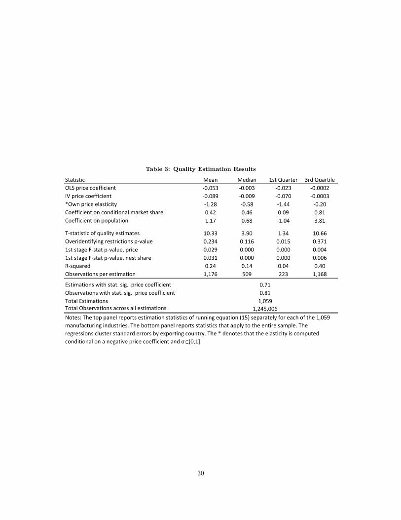
Table 3: Quality Estimation Results

Statistic Mean Median 1st Quarter 3rd QuartileOLS price coefficient ‐0.053 ‐0.003 ‐0.023 ‐0.0002IV price coefficient ‐0.089 ‐0.009 ‐0.070 ‐0.0003*Own price elasticity ‐1.28 ‐0.58 ‐1.44 ‐0.20Coefficient on conditional market share 0.42 0.46 0.09 0.81Coefficient on population 1.17 0.68 ‐1.04 3.81

T‐statistic of quality estimates 10.33 3.90 1.34 10.66Overidentifying restrictions p‐value 0.234 0.116 0.015 0.3711st stage F‐stat p‐value, price 0.029 0.000 0.000 0.0041st stage F‐stat p‐value, nest share 0.031 0.000 0.000 0.006R‐squared 0.24 0.14 0.04 0.40Observations per estimation 1,176 509 223 1,168

Estimations with stat. sig.  price coefficientObservations with stat. sig.  price coefficientTotal Estimations Total Observations across all estimations

0.710.811,059

1,245,006Notes: The top panel reports estimation statistics of running equation (15) separately for each of the 1,059 manufacturing industries. The bottom panel reports statistics that apply to the entire sample. The regressions cluster standard errors by exporting country. The * denotes that the elasticity is computed conditional on a negative price coefficient and σœ(0,1].

30

Table 4: Quality and Factor Endowments

Regressors (1) (2) (3) (4) (5)

Log (PCGDPct) 0.801 ***                       0.025 0.085 **

0.221                           0.054 0.036

Log (K/Lct)              0.804 ***         

             0.210             

Log (Educationct)                           0.274

                          0.207

China Dummy 0.783 ***0.081

Product x Year FEs yes yes yes yes yesR‐squared 0.20     0.21     0.32 0.49     0.49Observations 1,244,475     1,172,510    512,329 1,244,475     1,244,475

Unadjusted   Qualitycht Qualitycht

Notes: Table regresses the quality estimates on (log) per capita GDP, (log) capital‐labor ratios and percentage of workforce with tertiary education. Regressions include product‐year fixed effects. Robust standard errors are clustered by exporting country. Column 4 uses quality estimates that do not control for hidden varieties (qualities obtained from estimating equation (14)). Column 5 also uses the unadjusted quality measures and includes a China indicator variable. Regressions include product‐year fixed effects. Robust standard errors are clustered by exporting country. Significance levels: *** .01; ** .05; * .10. Source: World Bank's World Development Indicators.

31

Table 5: Relationship between Quality and Price

Regressors (1) (2)

Qualitycht ‐0.021 *   ‐0.025 *  

0.012     0.014    

Qualitycht x Log (Ladderh) 0.005 **  0.006 ** 

0.002     0.003    

Qualitycht x BW Sigmah 9.40E‐05 7.20E‐05

Product x Year FEs yes yesR‐squared 0.87 0.86Observations 1,245,006 1,165,703

ln(pricecht)

Notes: Column 1 regresses variety quality on (log) price and its interaction with the product's baseline quality ladder. Column 2 includes quality interacted with the elasticity of substitution measures obtained from Broda and Weintein (2004). Products with elasticities above the 90th percentile (elasticities greater than 76.9) are excluded. Robust standard errors are clustered by exporting country. Significance levels: *** .01; ** .05; * .10.

32

Table 6: Quality Ladder and Industry Characteristics

Regressors (1) (2) (3) (4)

Log (K/Lm) 0.133 **  0.124 **  0.138 ** 

0.051     0.057     0.060    

Log (Skillm) ‐0.015     ‐0.105     ‐0.121    

0.067     0.080     0.080    

Log (TFPm) 1.052 *   0.934     0.833    

0.600     0.577     0.580    

(Marketing Intensity)m          0.052 0.238          0.866 0.853

(R&D Itensity)m          6.036 ** 4.295          2.708 2.662

(Broda‐Weinstein Elasticity)m          0.016 0.015          0.011 0.011

(Coefficient of Variation of Unit Values)m 0.362 0.366 0.230 0.258

R‐squared 0.03     0.05 0.02     0.05Observations 325    306 325     306

Log (IndLadderm)

Notes: Column 1 regresses the industry quality ladder (defined in (20)) on four‐digit SIC factor intensities: capital intensity, skill intensity and total factor productivity. Capital intensity is the ratio of capital stock to total employment. Skill intensity is measured as the ratio of non‐production to production workers. Total factor productivity is obtained from a five‐factor model (Bartelsman et al., 1996). Factor intensities measured at 1989 values. Column 3 includes marketing expense to sales and R&D to sales ratios obtained from the 1975 FTC Line of Business survey. Column 3 includes industry‐level elasticity of substitution (obtain from Broda and Weinstein (2006)) and industry‐level coefficient of variation of unit values; these two product‐level variables are aggregated to the industry level using the same weights in (20). Robust standard errrors with significance levels: *** .01; ** .05; * .10.

33

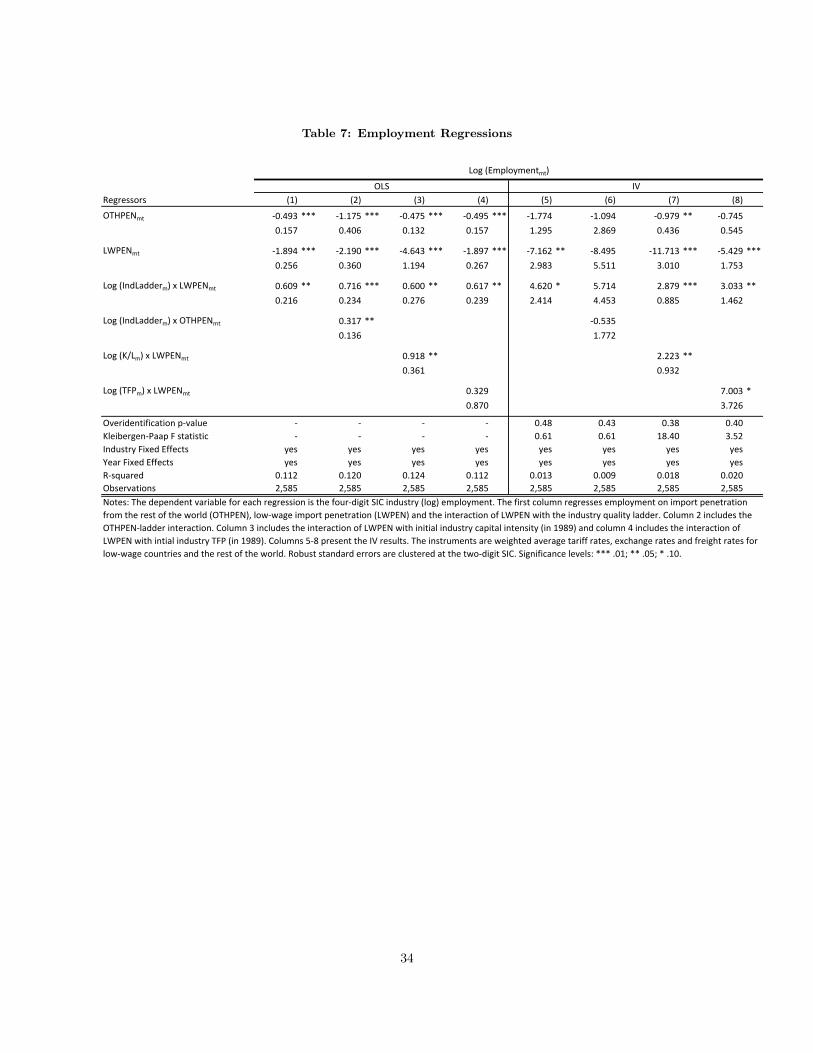
Table 7: Employment Regressions

Regressors (1) (2) (3) (4) (5) (6) (7) (8)

OTHPENmt ‐0.493 *** ‐1.175 *** ‐0.475 *** ‐0.495 *** ‐1.774     ‐1.094     ‐0.979 **  ‐0.745    

0.157     0.406     0.132     0.157     1.295     2.869     0.436     0.545    

LWPENmt ‐1.894 *** ‐2.190 *** ‐4.643 *** ‐1.897 *** ‐7.162 **  ‐8.495     ‐11.713 *** ‐5.429 ***

0.256     0.360     1.194     0.267     2.983     5.511     3.010     1.753    

Log (IndLadderm) x LWPENmt 0.609 **  0.716 *** 0.600 **  0.617 **  4.620 *   5.714     2.879 *** 3.033 ** 

0.216     0.234     0.276     0.239     2.414     4.453     0.885     1.462    

Log (IndLadderm) x OTHPENmt              0.317 **                                         ‐0.535                              

             0.136                                            1.772                              

Log (K/Lm) x LWPENmt                           0.918 **                                         2.223 **              

                          0.361                                            0.932                 

Log (TFPm) x LWPENmt                                        0.329                                            7.003 *  

                                       0.870                                            3.726    

Overidentification p‐value ‐ ‐ ‐ ‐ 0.48     0.43     0.38     0.40Kleibergen‐Paap F statistic ‐ ‐ ‐ ‐ 0.61     0.61     18.40     3.52Industry Fixed Effects yes yes yes yes yes yes yes yesYear Fixed Effects yes yes yes yes yes yes yes yesR‐squared 0.112     0.120     0.124     0.112 0.013 0.009 0.018 0.020Observations 2,585     2,585    2,585    2,585 2,585 2,585 2,585 2,585Notes: The dependent variable for each regression is the four‐digit SIC industry (log) employment. The first column regresses employment on import penetration from the rest of the world (OTHPEN), low‐wage import penetration (LWPEN) and the interaction of LWPEN with the industry quality ladder. Column 2 includes the OTHPEN‐ladder interaction. Column 3 includes the interaction of LWPEN with initial industry capital intensity (in 1989) and column 4 includes the interaction of LWPEN with intial industry TFP (in 1989). Columns 5‐8 present the IV results. The instruments are weighted average tariff rates, exchange rates and freight rates for low‐wage countries and the rest of the world. Robust standard errors are clustered at the two‐digit SIC. Significance levels: *** .01; ** .05; * .10.

Log (Employmentmt)

OLS IV

34

Table 8: Output Regressions

Regressors (1) (2) (3) (4) (5) (6) (7) (8)

OTHPENmt ‐0.508 **  ‐1.050 **  ‐0.485 **  ‐0.487 **  ‐0.430     1.159     0.231     0.321    

0.200     0.497     0.181     0.190     1.980     3.834     0.284     0.857    

LWPENmt ‐2.008 *** ‐2.243 *** ‐5.483 **  ‐1.978 *** ‐7.941 **  ‐11.054     ‐16.195 *** ‐6.619 ** 

0.354     0.404     1.942     0.281     4.016     7.713     3.593     2.603    

Log (IndLadderm) x LWPENmt 0.699 **  0.783 **  0.687 *   0.634 **  5.687 *   8.241     3.671 *** 4.439 ** 

0.307     0.308     0.367     0.301     3.227     6.300     1.371     1.971    

Log (IndLadderm) x OTHPENmt              0.252                                            ‐1.248                              

             0.186                                            2.178                              

Log (K/Lm) x LWPENmt                           1.160                                            3.562 ***             

                          0.749                                            1.379                 

Log (TFPm) x LWPENmt                                        ‐2.589 ***                                        8.813 *  

                                       0.800                                            4.973    

Overidentification p‐value ‐ ‐ ‐ ‐ 0.21    0.18     0.44    0.36Kleibergen‐Paap F‐statistic ‐ ‐ ‐ ‐ 0.61    0.61     18.40    3.52Industry Fixed Effects yes yes yes yes yes yes yes yesYear Fixed Effects yes yes yes yes yes yes yes yesR‐squared 0.181     0.185    0.195    0.184 0.006 0.003 0.016 0.015Observations 2,585     2,585    2,585    2,585 2,585 2,585 2,585 2,585

IV

Log (Outputmt)

OLS

Notes: The dependent variable for each regression is the four‐digit SIC industry (log) output. The first column regresses output on import penetration from the rest of the world (OTHPEN), low‐wage import penetration (LWPEN) and the interaction of LWPEN with the industry quality ladder. Column 2 includes the OTHPEN‐ladder interaction. Column 3 includes the interaction of LWPEN with initial industry capital intensity (in 1989) and column 4 includes the interaction of LWPEN with intial industry TFP (in 1989). Columns 5‐8 present the IV results. The instruments are weighted average tariff rates, exchange rates and freight rates for low‐wage countries and the rest of the world. Robust standard errors are clustered at the two‐digit SIC. Significance levels: *** .01; ** .05; * .10.

35

Table 9: Employment and Output Regressions, SIC2-Year Fixed Effects: IV

Regressors (1) (2) (3) (4) (5) (6)

OTHPENmt ‐0.720     ‐0.512     ‐0.499     ‐0.066     0.209     0.188    

1.234     0.496     0.675     1.529     0.345     0.699    

LWPENmt ‐4.398 *** ‐10.558 **  ‐4.531 *** ‐4.486 *** ‐13.000 *** ‐4.471 ** 

1.344     4.625     1.680     1.307     2.124     1.874    

Log (IndLadderm) x LWPENmt 2.706 **  2.148 **  2.764 **  3.275 **  2.082 **  3.045 ** 

1.360     0.954     1.357     1.590     1.059     1.204    

Log (K/Lm) x LWPENmt              2.121                               2.946 ***             

             1.440                               0.890                 

Log (TFPm) x LWPENmt                         6.777                            6.452   

                          4.717                               4.583    

Overidentification p‐value 0.36     0.35    0.59 0.281     0.339    0.435Kleibergen‐Paap F‐statistic 1.13     2.91    36.40 1.13     2.91    36.4Industry Fixed Effects yes yes yes yes yes yesTwo‐Digit SIC x Year FEs yes yes yes yes yes yesR‐squared 0.008 0.018 0.005 0.006 0.000 0.007Obs.  2,585 2,585 2,585 2,585 2,585 2,585

IV ‐ Log (Employmentm) IV ‐ Log (Outputm)

Notes: The dependent variables for each regression in columns 1‐3 and columns 4‐6 are the four‐digit SIC industry (log) employment and output, respectively. Each regression includes two‐digit SIC‐year pair fixed effects. The first column regresses employment on import penetration from the rest of the world (OTHPEN), low‐wage import penetration (LWPEN) and the interaction of LWPEN with the industry quality ladder. Column 2 includes the interaction of LWPEN with initial industry capital intensity (in 1989) and column 3 includes the interaction of LWPEN with intial industry TFP (in 1989). Columns 4‐6 present the IV results. The instruments are weighted average tariff rates, exchange rates and freight rates for low‐wage countries and the rest of the world. Robust standard errors are clustered at the two‐digit SIC. Significance levels: *** .01; ** .05; * .10.

36

Table 10: Employment Regressions, Robustness Checks

(1) Quality identified from baseline instruments and tariffs 0.501 *   2.755 ** 0.271     1.328    

(2) Product Count 0.000     ‐0.005    0.001     0.005    

(3) Variety Count ‐0.440     0.690    0.348     0.948    

(4) Price 1.285     7.436 *  1.227     4.129    

(5) Market Share 12.664 *** 21.512    3.415     21.914    

(6) Quality excluding residuals 0.646 *** 4.571 *  0.217     2.435    

(7) GDP‐Quality Ladder 0.992 ** 5.563 ***0.348     1.986    

(8) Broda‐Weinstein Ladder ‐0.910 *   ‐1.591    0.471     1.141    

(9) Exclude MFA products 0.484 ** 2.711 ** 0.232     1.378    

(10) Range 0.639 **  3.888 ***0.233     1.339    

(11) Inter‐quartile Range 0.650 **  5.236 ** 0.239     2.667    

(12) Standard Deviation 0.751 **  5.061 ** 0.271     2.417    

Notes: Table re‐runs the employment regression in equation (23) and reports the industry ladder interaction with LWPEN  coefficient for alternative definitions of the quality ladder. Row 1 re‐estimates equation (15) to include tariffs as additional instruments. Row 2 constructs the ladder from the number of countries (i.e., varieties) within the product and then aggregates to the industry according to equation (20). Row 3 counts the number of products within the four‐digit industry code. Rows 4 and 5 construct the ladder from the dispersion of prices and market shares within products, respectively. Row 6 defines the ladder from quality estimates exclusive of the residual: lcht = l1,ch+l2,t. Row 7 re‐runs equation (15) but uses GDP instead of population to control for hidden varieties. Row 8 constructs the quality ladder from the HS‐level elasticities of substitution estimated by Broda and Weinstein (2006). Row 9 excludes HS codes that were subject to quotas under the MFA in the construction of the industry ladders; the HS codes that were subject to quotas are taken from Brambilla, Khandelwal and Schott (2008). The remaining rows use the full range, inter‐quartile range and standard deviation of qualities within products. Robust standard errors are clustered at the two‐digit SIC for each regression. Significance levels: *** .01; ** .05; * .10.

IVRegression MethodOLSLWPEN ‐Ladder Interaction

37

Figure 1: Prices, Market Shares and Quality

−20

−10

010

20(L

og)

Pric

e/Q

uant

ity, Q

ualit

y

PH

L

CH

N

HK

G

IDN

ZA

F

IRL

TH

A

MY

S

ME

X

JPN

SG

P

FIN

SW

E

IND

TA

I

BR

A

KO

R

AU

T

AR

G

CH

E

GB

R

NO

R

NZ

L

ISR

ISL

CA

N

DE

U

ITA

NLD

JOR

FR

A

DN

K

TZ

A

AU

S

VE

N

Country

Price Quantity Quality Quality Best Fit

HS 8525203080Transmission Receivers Exceeding 400 MHZ

−5

05

10(L

og)

Pric

e/Q

uant

ity, Q

ualit

y

AR

GA

LB IND

ZA

FU

KR

CH

NLK

AT

AI

HK

GR

OM

PO

LID

NB

GR

UR

YB

RA

CO

LV

NM

DO

MB

LRP

AN

LBY

ES

PG

BR

GR

CM

AC

BH

ST

UR

ME

XT

UN

CZ

RK

OR

PH

LS

VN

ITA

TH

AD

NK

MC

DS

VK

NZ

LS

EN

MY

SK

NA

AU

SS

LVC

HE

PE

RS

WE

PR

TD

EU

CA

NS

LEH

UN

VE

NC

YP

MD

AM

AR

ISR

NLD

HR

VA

UT

FR

AB

EL

Country

Price Quantity Quality Quality Best Fit

HS 6403999065Footwear with Plastic Soles, Leather uppers

The graph plots countries’ export price, quantity and quality (with 95 percent confidence in-

terval) in HS 8525203080 (“Transmission Receivers Exceeding 400 MHZ”) and HS 6403999065

(“Footwear with Plastic Soles, Leather Uppers”) in 2001. Countries are ordered by unit value.

38