Embed Size (px)
Citation preview
Artville/GettyImages
CONGRESS OF THE UNITED STATESCONGRESSIONAL BUDGET OFFICE
A
CBOS T U D Y
DECEMBER 2005
The Long-TermBudget Outlook


CBO
The Long-TermBudget Outlook
December 2005
A
S T U D Y
The Congress of th
e United States O Congressional Budget Office
Notes
Unless otherwise indicated, the years referred to in this report are calendar years.
Numbers in the text and tables may not add up to totals because of rounding.
Preface
This Congressional Budget Office (CBO) report continues CBO’s examination of the pressures facing the federal budget over the coming decades and the kinds of policy choices that lawmakers confront as they consider ways to alleviate those pressures. If current policies continue, rapidly rising health care costs and an aging population will sharply increase federal spending for programs such as Social Security, Medicare, and Medicaid. This report presents illustrative scenarios for federal spending and revenues through 2050 and describes the impli-cations of those scenarios for the economy. In accordance with CBO’s mandate to provide objective, impartial analysis, this document contains no recommendations.
Ralph Smith coordinated the report and wrote major sections, as did Paul Cullinan, Douglas Hamilton, Noah Meyerson, Lyle Nelson, Benjamin Page, and David Weiner. Kevin Perese, Michael Simpson, and David Weiner provided the simulations, and Julie Topoleski made valuable contributions to the analysis. Many others at CBO provided helpful comments and assistance.
Christine Bogusz, Janey Cohen, Loretta Lettner, John Skeen, and Christian Spoor edited the manuscript. Maureen Costantino prepared the report for publication and produced the cover. Lenny Skutnik printed the initial copies of the report, and Annette Kalicki prepared the elec-tronic version for CBO’s Web site (www.cbo.gov).
Douglas Holtz-EakinDirector
December 2005


Contents
Executive Summary ix
1
Economic and Fiscal Implications of Federal Budgetary ChoicesOver the Long Run 1The Outlook for Federal Spending 4The Outlook for Revenues 4Alternative Scenarios for the Budget 5The Economic Effects of Growing Federal Debt 13
2
The Long-Term Outlook for Social Security 19The Outlook for Social Security Spending 19How Social Security Functions 19Options for Slowing the Growth of Social Security Spending 21
3
The Long-Term Outlook for Medicare and Medicaid 27Background on Medicare 27Background on Medicaid 28Growth in the Programs’ Costs 29Projections of the Programs’ Costs 31Options for Slowing Spending Growth 32

VI THE LONG-TERM BUDGET OUTLOOK
4
The Long-Term Outlook for Other Federal Spending 37Discretionary Spending 37Other Mandatory Spending 39
5
The Long-Term Outlook for Revenues 41The Past 50 Years 41Potential Future Paths for Federal Revenues 42Illustrative Revenue Paths 43
Appendix: Details of the Long-Term Budget Scenarios 47

CONTENTS VII
Tables
1-1.
Alternative Long-Term Paths for Primary Spending 101-2.
Projected Spending Under CBO’s Long-Term Budget Scenarios 122-1.
The Increase in Social Security’s Normal Retirement Age UnderCurrent Law and Under an Illustrative Option 243-1.
Medicare Spending by Type of Service, Fiscal Year 2004 283-2.
Distribution of Medicaid Enrollees and Benefit Payments byEligibility Category, Fiscal Year 2004 29A-1.
Assumptions Underlying CBO’s Long-Term Budget Scenarios 48Figures
1-1.
Total Federal Spending and Revenues Under CBO’s Long-TermBudget Scenarios 81-2.
Federal Debt Held by the Public Under CBO’s Long-Term BudgetScenarios 111-3.
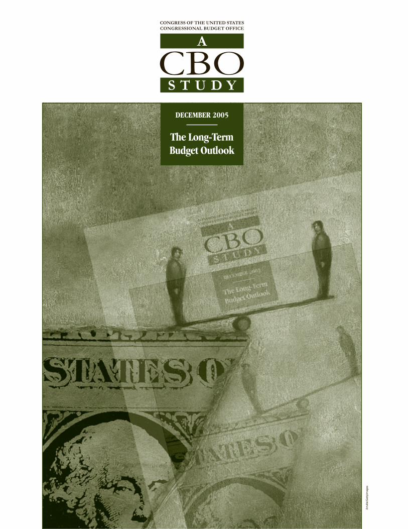
Federal Debt Held by the Public as a Percentage of GDP,1790 to 2004 162-1.
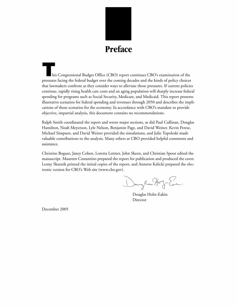
Spending for Social Security, 1962 to 2050 202-2.
The Population Age 65 or Older as a Percentage of the PopulationAges 20 to 64 212-3.
Federal Spending Under Current Law and Under Three IllustrativeOptions for Slowing the Growth of Social Security 233-1.
Sources of Medicare Cost Growth Since 1970 303-2.
Total Federal Spending for Medicare and Medicaid Under DifferentAssumptions About Excess Cost Growth 324-1.
Discretionary Spending, 1962 to 2005 384-2.
Mandatory Spending Other Than That for Social Security,Medicare, and Medicaid, 1962 to 2005 395-1.
Total Federal Revenues Under Alternative Paths 415-2.
Sources of Federal Revenues Over the Past 50 Years 425-3.
Individual Income Tax Liabilities Under Current Law and Under aPermanent Extension of EGTRRA and JGTRRA 44
viii THE LONG-TERM BUDGET OUTLOOK
5-4.
Individual Income Tax Liabilities Under Current Law and Under aModified AMT 445-5.
Individual Income Tax Liabilities Under Three Policy Alternatives 455-6.
The AMT’s Impact on Individual Income Tax Liabilities UnderCurrent Law 455-7.
Individual Income Taxes and Payroll Taxes Under the Current-Lawand Historical-Average Scenarios 46A-1.
Social Security Spending Under CBO’s Long-Term Budget Scenarios 50A-2.
Medicare Spending Under CBO’s Long-Term Budget Scenarios 51A-3.
Federal Medicaid Spending Under CBO’s Long-Term Budget Scenarios 52A-4.
Defense Spending Under CBO’s Long-Term Budget Scenarios 53A-5.
Other Federal Spending Under CBO’s Long-Term Budget Scenarios 54A-6.
Federal Interest Spending Under CBO’s Long-Term Budget Scenarios 55A-7.
Individual Income Tax Revenues Under CBO’s Long-Term Budget Scenarios 56A-8.
Real Gross Domestic Product Under CBO’s Long-Term BudgetScenarios 57A-9.
Total Surplus or Deficit Under CBO’s Long-Term Budget Scenarios 58Boxes
1-1.
Why Is Federal Debt Held by the Public Important? 21-2.
The Impact of Immigration on the Long-Term Budget Outlook 31-3.
The Growth of Health Care Costs 6Figures (Continued)

Executive Summary
As health care costs continue to grow faster than the economy and the baby-boom generation nears eligi-bility for Social Security and Medicare, the United States faces inevitable decisions about the fundamentals of its spending policies and its means of financing those poli-cies. This Congressional Budget Office report looks at a range of possible paths for federal spending and revenues through 2050 and combines them into various hypothet-ical scenarios. Analysis of the scenarios suggests the fol-lowing conclusions:
B Driven by rising health care costs and an aging popu-lation, federal spending for Medicare, Medicaid, and Social Security will claim a sharply increasing share of the nation’s economic output over the coming decades.
B Even if taxation reached levels that were unprece-dented in the United States, current spending policies could become financially unsustainable. An ever- growing burden of federal debt held by the public would have a corrosive and potentially contractionary effect on the economy.
B As the U.S. tax system is now configured, federal reve-nues will grow faster than the overall economy. Under current law, taxpayers will face higher rates, with detri-mental consequences for work, saving, and economic growth.
B Fiscal policy could be financially sustainable if the growth of health care costs slowed significantly from historical rates. But even in that case, tax revenues would probably need to be higher than they have been in the past, unless the growth of other spending was curbed.
B If taxation is restricted to the levels that prevailed in the past, the growth of spending on programs for the elderly will have to be reduced substantially. Limiting the growth of outlays for defense, education, transpor-tation, and other discretionary programs would not be enough to ensure fiscal sustainability.
B Likewise, economic growth alone is unlikely to bring the nation’s long-term fiscal position into balance. Moreover, issuing ever-larger amounts of debt or dra-matically raising tax rates could significantly reduce economic growth.


C HA P T E R
1Economic and Fiscal Implications of Federal
Budgetary Choices Over the Long RunChapter 1: Economic and Fiscal Implications of Federal Budgetary Choices Over the Long Run
Over the next half-century, the United States will confront the challenge of conducting its fiscal policy in the face of the retirement of the baby-boom generation (the large number of people born between 1946 and 1964).1 Under current policies, the aging of the popula-tion is likely to combine with rapidly rising health care costs to create an ever-growing demand for resources to finance federal spending for mandatory programs, such as Medicare, Medicaid, and Social Security. This report pre-sents several illustrative scenarios for federal spending and revenues through mid-century, describes their implica-tions for the economy, and frames the key issues involved in choosing among those alternatives. The analysis indi-cates that attaining fiscal stability in the coming decades will probably require substantial reductions in the pro-jected growth of spending and perhaps also a sizable increase in taxes as a share of the economy.
The scenarios suggest that the nation’s broad fiscal stance through 2050 will depend mainly on two factors: the growth rate of health care costs and the willingness of the populace to be taxed. On the spending side of the budget, the growth of costs for the government’s major health care programs is the largest source of budgetary uncer-tainty.2 The growth rates used in these scenarios suggest that total federal spending for Medicare and Medicaid in 2050 could range anywhere from 7 percent of gross domestic product (GDP)—a measure of national eco-nomic resources—to 22 percent, though under current
1. For a definition of fiscal policy and other terms used in this report, see the Congressional Budget Office’s glossary of budgetary and economic terms, available at www.cbo.gov.
2. The future path of productivity growth and other economic fac-tors are also uncertain and will have budgetary consequences. However, to simplify the presentation, those sources of uncer-tainty are not analyzed in this report.
law, spending at the low end of that range is unlikely. In 2005, by comparison, such spending equaled 4.2 percent of GDP.
Projected spending for the Social Security program grows more slowly and is far more predictable. Other federal spending (for national defense and a wide variety of non-defense programs) is a far smaller source of budgetary pressure and contributes less to the uncertainty about future federal spending. Even under a variety of assump-tions, the range of projected spending as a percentage of GDP envisioned for those programs does not approach the size of the range projected for Medicare and Medicaid spending.
On the revenue side of the budget, the two long-term paths considered in this report suggest a smaller, though significant, range of outcomes. In those paths—which assume either enactment of legislative changes to keep receipts at their historical average level relative to GDP or continued adherence to current tax law—revenues range from 18.3 percent to 23.7 percent of GDP in 2050, com-pared with about 17.5 percent in 2005.
A useful barometer of fiscal policy is the amount of gov-ernment debt held by the public as a percentage of GDP. (For a discussion of why such debt is important, seeBox 1-1.) By that measure, different budgetary assump-tions can lead to vastly different outcomes in 2050. The alternative spending paths considered in this report diverge primarily after 2015, and some of those paths lead to growth in debt that is not sustainable over the long run.
The path of fiscal policy is not an end in itself. It matters because of its impact on people and the economy. Mini-mizing harmful economic effects would require con-
2 THE LONG-TERM BUDGET OUTLOOK
Box 1-1.
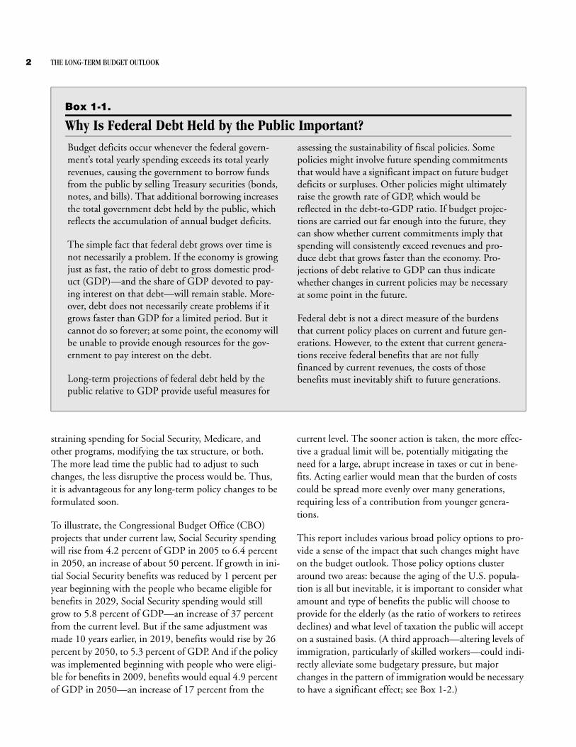
Why Is Federal Debt Held by the Public Important?Budget deficits occur whenever the federal govern-ment’s total yearly spending exceeds its total yearly revenues, causing the government to borrow funds from the public by selling Treasury securities (bonds, notes, and bills). That additional borrowing increases the total government debt held by the public, which reflects the accumulation of annual budget deficits.
The simple fact that federal debt grows over time is not necessarily a problem. If the economy is growing just as fast, the ratio of debt to gross domestic prod-uct (GDP)—and the share of GDP devoted to pay-ing interest on that debt—will remain stable. More-over, debt does not necessarily create problems if it grows faster than GDP for a limited period. But it cannot do so forever; at some point, the economy will be unable to provide enough resources for the gov-ernment to pay interest on the debt.
Long-term projections of federal debt held by the public relative to GDP provide useful measures for
assessing the sustainability of fiscal policies. Some policies might involve future spending commitments that would have a significant impact on future budget deficits or surpluses. Other policies might ultimately raise the growth rate of GDP, which would be reflected in the debt-to-GDP ratio. If budget projec-tions are carried out far enough into the future, they can show whether current commitments imply that spending will consistently exceed revenues and pro-duce debt that grows faster than the economy. Pro-jections of debt relative to GDP can thus indicate whether changes in current policies may be necessary at some point in the future.
Federal debt is not a direct measure of the burdens that current policy places on current and future gen-erations. However, to the extent that current genera-tions receive federal benefits that are not fully financed by current revenues, the costs of those benefits must inevitably shift to future generations.
straining spending for Social Security, Medicare, and other programs, modifying the tax structure, or both. The more lead time the public had to adjust to such changes, the less disruptive the process would be. Thus, it is advantageous for any long-term policy changes to be formulated soon.
To illustrate, the Congressional Budget Office (CBO) projects that under current law, Social Security spending will rise from 4.2 percent of GDP in 2005 to 6.4 percent in 2050, an increase of about 50 percent. If growth in ini-tial Social Security benefits was reduced by 1 percent per year beginning with the people who became eligible for benefits in 2029, Social Security spending would still grow to 5.8 percent of GDP—an increase of 37 percent from the current level. But if the same adjustment was made 10 years earlier, in 2019, benefits would rise by 26 percent by 2050, to 5.3 percent of GDP. And if the policy was implemented beginning with people who were eligi-ble for benefits in 2009, benefits would equal 4.9 percent of GDP in 2050—an increase of 17 percent from the
current level. The sooner action is taken, the more effec-tive a gradual limit will be, potentially mitigating the need for a large, abrupt increase in taxes or cut in bene-fits. Acting earlier would mean that the burden of costs could be spread more evenly over many generations, requiring less of a contribution from younger genera-tions.
This report includes various broad policy options to pro-vide a sense of the impact that such changes might have on the budget outlook. Those policy options cluster around two areas: because the aging of the U.S. popula-tion is all but inevitable, it is important to consider what amount and type of benefits the public will choose to provide for the elderly (as the ratio of workers to retirees declines) and what level of taxation the public will accept on a sustained basis. (A third approach—altering levels of immigration, particularly of skilled workers—could indi-rectly alleviate some budgetary pressure, but major changes in the pattern of immigration would be necessary to have a significant effect; see Box 1-2.)

CHAPTER ONE ECONOMIC AND FISCAL IMPLICATIONS OF FEDERAL BUDGETARY CHOICES OVER THE LONG RUN 3
Box 1-2.
The Impact of Immigration on the Long-Term Budget OutlookSome analysts argue that the budgetary effects of the aging of the population could be alleviated by an increase in immigration. Immigrants pay a variety of taxes. However, their presence also tends to raise spending, because immigrants and their children benefit from various government programs.1
Evaluating the net effect of immigration on the bud-get is complicated by the fact that immigrants, on average, may differ from native-born people in a vari-ety of ways. For example, immigrants tend to have lower incomes than native-born people do, so they may generate less tax revenue and receive more bene-fits from need-based programs such as Medicaid and Food Stamps. They also tend to have more children than their native-born counterparts do—meaning that in the short run they may create more demand for public education and other programs aimed at children but that in the long run they leave moredescendants, who in turn pay taxes and receive gov-ernment services.
The Congressional Budget Office (CBO) has re-viewed research by numerous analysts on how immi-gration affects government finances.2 The research focuses primarily on the effects on federal, state, and
local government budgets taken together, because those effects are most relevant to the impact on the overall economy. However, the results are suggestive for federal finances as well. In some cases, the as-sumptions that those analysts used to project spend-ing and revenues far into the future differ from the assumptions that CBO uses in this study, so the results must be viewed with caution. Nevertheless, under the assumptions used in that research, two main conclusions emerge:
B Changes in rates of immigration—within reason-able ranges—are unlikely to substantially offset the budgetary impact of the aging of the U.S. population and rising health care costs, if the aver-age characteristics of immigrants remain as they have been in the past. For example, studies suggest that doubling the current flow of about 1 million net immigrants to the United States per year would probably fill only a small portion of the prospective gap between government spending and revenues. The estimated impact differs by jurisdiction: studies tend to estimate modest posi-tive effects on federal finances but modest negative effects on state and local finances.
B Increases in the immigration of skilled workers—those with college degrees—could have a signifi-cant positive impact on the long-term financial outlook for federal, state, and local governments taken together, but those increases would have to be substantial. Roughly one-third of current legal immigrants to the United States have at least a bachelor’s degree. One paper estimates that if the number of such “skilled” immigrants between the ages of 25 and 49 increased more than tenfold to 1.8 million per year, projected long-term revenues would be sufficient to cover projected spending despite the aging of the population and growth in health care costs. However, that estimate assumes that the immigrants would bring no dependent children with them.
1. For analysis of other issues relating to immigration or the aging of populations, see Congressional Budget Office, A Description of the Immigrant Population (November 2004), The Role of Immigrants in the U.S. Labor Market (November 2005), and Global Population Aging in the 21st Century and Its Economic Implications (December 2005).
2. See, for example, Alan J. Auerbach and Philip Oreopoulis, “Analyzing the Fiscal Impact of U.S. Immigration,” American Economic Review, vol. 89, no. 2 (May 1999); Ronald Lee and Timothy Miller, “Immigration, Social Security, and Broader Fiscal Impacts,” American Economic Review, vol. 90, no. 2 (May 2000); Kjetil Storesletten, “Sustaining Fiscal Policy Through Immigration,” Journal of Political Economy, vol. 108, no. 2 (April 2000); and Hans Fehr, Sabine Jokisch, and Laurence Kotlikoff, The Role of Immigration in Dealing with the Developed World’s Demographic Transition, Working Paper No. 10512 (Cambridge, Mass.: National Bureau of Eco-nomic Research, May 2004).

4 THE LONG-TERM BUDGET OUTLOOK
The Outlook for Federal SpendingFor much of its history, the United States devoted only a small fraction of its resources to the activities of the fed-eral government. But the second half of the 20th century marked a period of sustained higher levels of federal peacetime spending. For the past 50 years, federal outlays have averaged about 20 percent of GDP. In 2005, those outlays totaled $2.5 trillion.
Not only has the amount of spending grown, but its com-position has changed dramatically. Spending for manda-tory programs has increased from less than one-third of total federal spending in the early 1960s to more than one-half in recent years. Most of that growth has been concentrated in Social Security, Medicare, and Medicaid. Together, those programs now account for about 42 per-cent of federal outlays, compared with 2 percent in 1950 (before the health programs were created) and 25 percent in 1975.
The retirement of the baby-boom generation portends a significant, long-lasting shift in the age profile of the U.S. population, which will dramatically alter the balance between the working-age and retirement-age components of that population. The share of people age 65 or older is projected to grow from 12 percent in 2005 to 19 percent by 2030, while the share of people ages 20 to 64 is expected to fall from 60 percent to 56 percent. As a result, CBO projects that the number of workers per Social Security beneficiary will decline significantly over the next three decades: from about 3.3 now to 2.1 in 2030. Unless immigration or fertility rates change sub-stantially, that figure will continue to decrease slowly after 2030. The interaction of growth in the retired population and the current structure of the Social Security program leads CBO to project that the cost of Social Security ben-efits will rise from 4.2 percent of GDP now to 6.0 per-cent in 2030.
The future growth of Social Security costs, however, pales next to the likely increases in costs for the government’s major health care programs: Medicare and Medicaid. Ris-ing health care costs are boosting spending for those pro-grams to a greater degree than can be explained by increases in enrollment and general inflation alone. Since 1970, all factors (including policy changes) have caused annual costs per Medicare enrollee to grow 2.9 percent-age points faster than per capita GDP, on average—a dif-ference referred to as “excess cost growth” (see Box 1-3 on
page 6). If that growth remained high—for example, 2.5 percentage points, as some of the scenarios in this report assume—the federal government’s total spending for Medicare and Medicaid would reach 22 percent of GDP by 2050, compared with 4.2 percent in 2005.3 The Medicare trustees assume that excess cost growth will decline to 1 percentage point. Even at that rate, however, the total federal costs of Medicare and Medicaid would climb to 12.6 percent of GDP by 2050.
Spending for other federal programs could fall as a per-centage of GDP in future years, offsetting some of the growth associated with Social Security, Medicare, and Medicaid. However, as currently structured, those three programs are still likely to raise total federal spending rel-ative to GDP in coming decades.
The Outlook for RevenuesLike federal spending, revenues have been significantly higher in the past half-century than in previous eras—fluctuating between 16.1 percent and 20.9 percent of GDP since 1951.4 And just as spending priorities have changed during that period, the composition of revenues has shifted. Social insurance payroll taxes (for Social Security, Medicare, unemployment insurance, and retire-ment programs for federal civilian employees) have risen along with the size of the underlying programs, while cor-porate income taxes and excise taxes have diminished as shares of total receipts.
This report examines two long-term paths for federal rev-enues. In the first, revenues level off at 18.3 percent of GDP, the average for the past 30 years.5 In the second, revenues follow the path implied by current tax law (in-cluding the scheduled rise in taxes with the expiration of tax laws enacted in 2001 and 2003). The latter assump-
3. Projections of future Medicare and Medicaid spending in this report incorporate the effects of the Medicare prescription drug benefit, which begins in January 2006.
4. Revenues have exceeded 19.5 percent of GDP on only three occa-sions in the past 50 years: 1969, 1981, and 1998 through 2001. The first instance resulted from a one-year income tax surcharge of 10 percent; the second was largely attributable to inflation-related bracket creep in the late 1970s and early 1980s; and the third was heavily affected by historically large capital gains realiza-tions.
5. Federal revenues have averaged 18.7 percent of GDP for the past 10 years and 18.3 percent for both the past 20 and past 30 years.

CHAPTER ONE ECONOMIC AND FISCAL IMPLICATIONS OF FEDERAL BUDGETARY CHOICES OVER THE LONG RUN 5
tion implies that average tax rates for individuals will rise well above any historical levels as both inflation and the real growth of income (growth above and beyond infla-tion) cause a large share of taxpayers to become subject to the alternative minimum tax (AMT) or to move into higher tax-rate brackets. In that path, revenues rise to 23.7 percent of GDP by 2050.
Of course, decisions about taxes and spending interact. Pressures on the spending side of the budget could make it very difficult to avoid raising taxes beyond their histori-cal share of GDP to help forestall significant increases in federal debt.
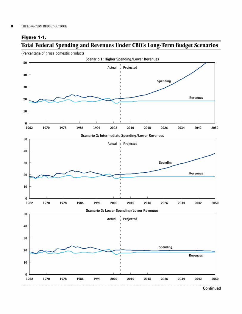
Alternative Scenarios for the BudgetTo illustrate the possible range of long-term budgetary outcomes, CBO projected federal spending and revenues through 2050 under a variety of assumptions. It com-bined those projections into six broad scenarios (see Fig-ure 1-1 on page 8 and Tables 1-1 and 1-2 on pages 10 and 12). The scenarios consist of combinations of three different spending paths and two revenue projections, as shown below:
The scenarios are designed to capture the broad long-term dimensions of the fiscal choices that the Congress could face in coming years and the budgetary and eco-nomic implications of those choices. Each revenue or spending path is a possible representation of current pol-icy or of long-term historical experience. However, one or more of the combinations are probably unrealistic in that they represent a mismatch between the levels of taxation and spending that would eventually be addressed by pol-icy changes.6 Also, the scenarios for the Social Security and Medicare programs were constructed without regard
Scenario 1 Higher Spending/Lower Revenues
Scenario 2 Intermediate Spending/Lower Revenues
Scenario 3 Lower Spending/Lower Revenues
Scenario 4 Higher Spending/Higher Revenues
Scenario 5 Intermediate Spending/Higher Revenues
Scenario 6 Lower Spending/Higher Revenues
to any limits on spending that may arise if those pro-grams’ trust funds are depleted.
Assumptions About Spending and Revenues over the Long TermThe three spending paths combine different assumptions about the future costs of major federal health programs, national defense, and nondefense programs:
B The higher-spending path assumes that excess cost growth in Medicare and Medicaid continues at past rates (2.5 percentage points per year), that defense spending follows the Administration’s 2006 Future Years Defense Program (with allowances for cost risks and additional spending to support the war on terror-ism) through 2024,7 and that nondefense discretion-ary spending and other mandatory spending (except for Social Security and interest on federal debt held by the public) remain at their historical levels as a share of GDP.
B The intermediate-spending trajectory differs from the high path in two ways: the rate of excess cost growth declines to 1.0 percentage point (as the Medicare trustees assume), and defense spending gradually returns to its historical real level.
B The lower-spending path differs from the intermedi-ate path in three ways: no excess cost growth occurs in health care programs, other mandatory spending slowly declines as a percentage of GDP, and non-defense discretionary spending remains at a constant real level (that is, the current level of spending adjusted for inflation).
All of those paths use the same projection of Social Secu-rity spending, which is calculated under the assumption that all currently scheduled benefits will be paid.
6. Likewise, no attempt was made to take into account potential interactions between the assumptions underlying future spending paths and revenues. For example, higher growth in health care spending could result in a larger percentage of workers’ total com-pensation coming in the form of untaxed employer-sponsored health insurance rather than in taxable wages.
7. For more details, see Congressional Budget Office, The Long-Term Implications of Current Defense Plans and Alternatives: Summary Update for Fiscal Year 2006 (October 2005).

6 THE LONG-TERM BUDGET OUTLOOK
Box 1-3.
The Growth of Health Care CostsTotal health care spending in the United States has been growing faster than the economy for many years, and it is projected to continue doing so. Between 1960 and 2003, national health expendi-tures (NHE) increased from 5.1 percent of gross domestic product (GDP) to 15.3 percent—the result of an average annual growth rate that was 2.6 per-centage points higher than that of the economy as a whole. The gap between the two growth rates has decreased somewhat over time. It has narrowed par-ticularly since 1990, as the numbers below indicate. That period has been unusual, however, in that NHE grew at approximately the same rate as the economy for seven years (from 1993 to 2000) and then acceler-ated rapidly.
Growth in health care spending has outstripped eco-nomic growth regardless of the source of its funding. Expenditures from public sources (government pro-grams such as Medicare and Medicaid) and private sources (private-sector health insurance or out-of-pocket spending) have both risen faster than GDP. The major factor associated with that growth has been the development and increasing use of new medical technology, which has been fueled in part by the prevalence of health insurance coverage. In the health care field, unlike in many sectors of the econ-omy, technological advances have generally raised costs rather than lowered them. Widely available health insurance coverage—both public and pri-vate—means that individual consumers have little incentive to restrict their consumption of services, because the price they face is far lower than the cost of providing the service. In addition, some tax prefer-
ences encourage the purchase of insurance, and oth-ers lower the effective price of health services.
MedicareThe total cost of the Medicare program has been growing faster than the economy for decades, although that growth has been slowing over time (see the table at right). As a result, spending for the pro-gram increased from 0.7 percent of GDP in 1970 to 2.7 percent in 2005.
Medicare costs have grown in part because of increased enrollment. More important, with growth related to demographic changes excluded, costs per enrollee still rose 2.9 percentage points faster than per capita GDP over the 1970-2004 period. That “excess cost growth” has resulted primarily from the same factors that have caused health care spending in the nation as a whole to grow more rapidly than the economy—most notably, utilization of new medical technology. If the 1970s are excluded, the average rate of excess cost growth is smaller: 2.3 percentage points. (Implementation of the prospective payment system for inpatient hospital care in 1983 was an important factor that helped slow the growth of Medicare costs per beneficiary.) The average rate of excess cost growth is still smaller—1.9 percentage points—if it includes only 1990 to 2004, a period when cost growth was especially volatile. The growth of Medicare spending decelerated rapidly in the late 1990s and then rebounded, partly in response to leg-islative changes that introduced cost containment measures and later overturned them. The implemen-tation of the voluntary prescription drug benefit in 2006 will cause a one-time spike in the growth of spending per beneficiary. If excess cost growth con-tinues at any of the historical rates, it will dramati-cally increase Medicare spending as a share of both the federal budget and the economy.
MedicaidFederal spending for the joint federal/state Medicaid program has also grown faster than the economy for decades, rising from 0.3 percent of GDP in 1970 to
Average Annual DifferenceBetween Growth of NHE
and Growth of GDP(Percentage points)
1960-2003 2.61970-2003 2.41980-2003 2.41990-2003 1.9

CHAPTER ONE ECONOMIC AND FISCAL IMPLICATIONS OF FEDERAL BUDGETARY CHOICES OVER THE LONG RUN 7
Box 1-3.
Continued1.5 percent in 2005. That rise has been driven by increased enrollment and growth in spending per enrollee. Since 1975 (the earliest year for which data on Medicaid enrollment are readily available), Medic-aid spending per enrollee has grown an average of 2.4 percentage points faster than per capita GDP. The average gap between the two growth rates was 1.6 percentage points over the 1980-2004 period and 1.4 percentage points over the 1990-2004 period. That narrowing of the gap has resulted in part from large increases in enrollment among children and families, who have much lower per capita costs than other eligible groups do. (Unlike the estimates for Medicare, the analysis of growth in Medicaid costs relative to per capita GDP did not remove the effects of demographic changes in the enrolled population.)
The growth of Medicaid costs per enrollee is attribut-able to various factors. First, the program has ex-panded over the years (for example, optional services have been added under state plans). Second, as with
Medicare and private health spending, utilization of new technology has boosted Medicaid costs as health care providers have supplied beneficiaries with more tests and treatments. Prescription drugs are a particu-lar example, and their usage has been a major factor driving up costs, especially in recent years. Finally, in addition to services provided directly to Medicaid enrollees, states’ efforts to maximize federal reim-bursements have boosted federal spending at times.
Outlook for the FutureHow long health care costs can continue to grow significantly faster than the economy is a matter for speculation. If past growth rates persist, spending for health care will eventually consume such a large share of the nation’s output that real (inflation-adjusted) spending on other goods and services will have to decline sharply. There is no evidence to suggest that excess cost growth will slow significantly in the short run. Moreover, some level of excess cost growth is likely to continue for some time to come.
Growth in the Medicare and Medicaid Programs
Source: Congressional Budget Office.
a. Medicare data are for calendar years; Medicaid data are for fiscal years.
b. The measure of enrollment used for Medicare reflects the effects on costs of the changing composition of Medicare beneficia-ries; the measure of enrollment used for Medicaid does not. The latter measure is based on administrative data from the Centers for Medicare and Medicaid Services.
c. Excess cost growth is one plus the growth rate of outlays per enrollee divided by one plus the growth rate of per capita GDP, minus one. For example, (1.094 ÷ 1.063) - 1 = 0.029.
Yearsa
1970-2004 11.5 2.0 9.4 6.3 2.91980-2004 9.2 1.6 7.5 5.1 2.31990-2004 7.5 1.4 6.0 4.1 1.9
1975-2004 12.1 3.3 8.5 6.0 2.41980-2004 11.1 4.0 6.8 5.1 1.61990-2004 11.0 5.0 5.6 4.1 1.4
Average Annual
Medicare
Medicaid
Domestic ProductExcess Cost
Growthc
PercentageGrowth in
Federal Outlays
PercentageGrowth in
per Enrollee
PercentageGrowth in
Federal Outlays
PercentageGrowth in
Enrollmentbper Capita Gross
8 THE LONG-TERM BUDGET OUTLOOK
Figure 1-1.
Total Federal Spending and Revenues Under CBO’s Long-Term Budget Scenarios(Percentage of gross domestic product)
Continued
1962 1970 1978 1986 1994 2002 2010 2018 2026 2034 2042 20500
10
20
30
40
50
Revenues
Spending
Actual Projected
Scenario 1: Higher Spending/Lower Revenues
1962 1970 1978 1986 1994 2002 2010 2018 2026 2034 2042 20500
10
20
30
40
50
Revenues
Actual Projected
1962 1970 1978 1986 1994 2002 2010 2018 2026 2034 2042 20500
10
20
30
40
50
Spending
Revenues
Actual Projected
Scenario 2: Intermediate Spending/Lower Revenues
Spending
Scenario 3: Lower Spending/Lower Revenues

CHAPTER ONE ECONOMIC AND FISCAL IMPLICATIONS OF FEDERAL BUDGETARY CHOICES OVER THE LONG RUN 9
Figure 1-1.
Continued (Percentage of gross domestic product)
Source: Congressional Budget Office.
Notes: For information about the assumptions underlying these scenarios, see Table A-1 in the appendix.
Spending includes net interest.
1962 1970 1978 1986 1994 2002 2010 2018 2026 2034 2042 20500
10
20
30
40
50
Revenues
Spending
Actual Projected
1962 1970 1978 1986 1994 2002 2010 2018 2026 2034 2042 20500
10
20
30
40
50
Revenues
Spending
Actual Projected
1962 1970 1978 1986 1994 2002 2010 2018 2026 2034 2042 20500
10
20
30
40
50
Spending
Revenues
Actual Projected
Scenario 4: Higher Spending/Higher Revenues
Scenario 5: Intermediate Spending/Higher Revenues
Scenario 6: Lower Spending/Higher Revenues

10 THE LONG-TERM BUDGET OUTLOOK
Table 1-1.
Alternative Long-Term Paths for Primary Spending (Percentage of gross domestic product)
Source: Congressional Budget Office.
Note: Primary spending is the sum of spending for defense, Social Security, Medicare, Medicaid, and other spending (except interest).
a. Minor differences in simulated gross domestic product (GDP) result in small differences among the paths in Social Security spending as a percentage of GDP and between the intermediate-spending path and the lower-spending path in defense spending.
b. Other spending is lower in 2030 and 2050 under the higher-spending path than under the intermediate-spending path because this cate-gory includes premiums paid by Medicare enrollees, which are treated as negative outlays. Those premiums are larger under the higher path’s assumption that excess cost growth is 2.5 percentage points.
Higher-Spending Path3.5 2.7 2.04.2 6.0 6.65.3 12.0 21.95.8 5.0 4.0____ ____ ____
Total 18.9 25.6 34.4
Intermediate-Spending Path3.4 2.0 1.54.2 6.0 6.45.0 9.2 12.65.8 5.3 4.9____ ____ ____
Total 18.4 22.5 25.3
Lower-Spending Path3.4 2.0 1.44.2 5.9 6.34.7 6.2 7.05.5 3.8 2.7____ ____ ____
Total 17.9 17.9 17.3
Social SecurityMedicare and MedicaidOtherb
DefenseSocial SecurityMedicare and MedicaidOtherb
2010 2030a 2050a
DefenseSocial SecurityMedicare and MedicaidOther
Defense
As noted above, the six scenarios incorporate two trajec-tories for revenues:
B The lower-revenue path assumes that revenues slowly climb from their present level until they reach 18.3 percent of GDP in 2014—the average level of the past 30 years—and then remain there through 2050.
B The higher-revenue path approximates an extension of current law governing the individual income tax. In that path, real bracket creep (real income growth pushing taxpayers into higher tax brackets) and the AMT cause total revenues to continually rise until they reach 23.7 percent of GDP in 2050.
More details about the assumptions and projections underlying the scenarios are shown in the appendix.
Detailed year-by-year spending and revenue projections under the six scenarios and information about the eco-nomic assumptions underlying the scenarios will be avail-able on CBO’s Web site (www.cbo.gov).
Implications of the ScenariosMeasured in terms of federal debt, the scenarios that as-sume that revenues level off at 18.3 percent of GDP (sce-narios 1 through 3) are not promising (see Figure 1-2). Of those, only the lower-spending/lower-revenue alterna-tive (scenario 3) is sustainable over the long term, and that path assumes no excess cost growth in health care programs—an unlikely prospect. Under the other two of those scenarios (higher-spending/lower-revenue and

CHAPTER ONE ECONOMIC AND FISCAL IMPLICATIONS OF FEDERAL BUDGETARY CHOICES OVER THE LONG RUN 11
Figure 1-2.
Federal Debt Held by the Public Under CBO’s Long-Term Budget Scenarios (Percentage of gross domestic product)
Source: Congressional Budget Office.
Notes: Scenario 1 = higher spending/lower revenues
Scenario 2 = intermediate spending/lower revenues
Scenario 3 = lower spending/lower revenues
Scenario 4 = higher spending/higher revenues
Scenario 5 = intermediate spending/higher revenues
Scenario 6 = lower spending/higher revenues
For information about the assumptions underlying these scenarios, see Table A-1 in the appendix.
1962 1970 1978 1986 1994 2002 2010 2018 2026 2034 2042 2050-150
-100
-50
0
50
100
150
200
Scenario 1
Scenario 5
Scenario 4
Scenario 3
Scenario 6
Scenario 2Actual Projected
intermediate-spending/lower revenue), federal deficits grow steadily relative to the size of the economy. As a result, debt reaches nearly 140 percent of GDP by 2030 in scenario 1 or nearly 100 percent of GDP in scenario 2 and continues to grow steadily thereafter (even without taking into account the harmful effects of long-term defi-cits on economic growth, which are not included in the scenarios but are discussed later in this chapter).
If revenues are higher—as they would be under an exten-sion of current law—the outlook for federal debt is bet-ter, but fiscal stability is not assured. The higher-spending/higher-revenue path (scenario 4) still yields rapidly rising deficits. The intermediate-spending/higher-revenue path (scenario 5) comes closer to balancing reve-
nues and spending, but it would require further increases in taxes or reductions in the growth of spending to pro-duce a stable debt-to-GDP ratio. Under that scenario, noninterest outlays exceed revenues by 1.6 percent by 2050. Only the lower-spending/higher-revenue path (sce-nario 6)—which assumes no excess cost growth in health care programs—produces a declining debt-to-GDP ratio.8
The most critical assumption in choosing which spend-ing paths are the most likely is the amount of excess cost
8. The long-term pressures on the federal budget illustrated by those scenarios are slightly greater than the ones that CBO presented two years ago in Congressional Budget Office, The Long-Term Budget Outlook (December 2003).
12 THE LONG-TERM BUDGET OUTLOOK
Table 1-2.
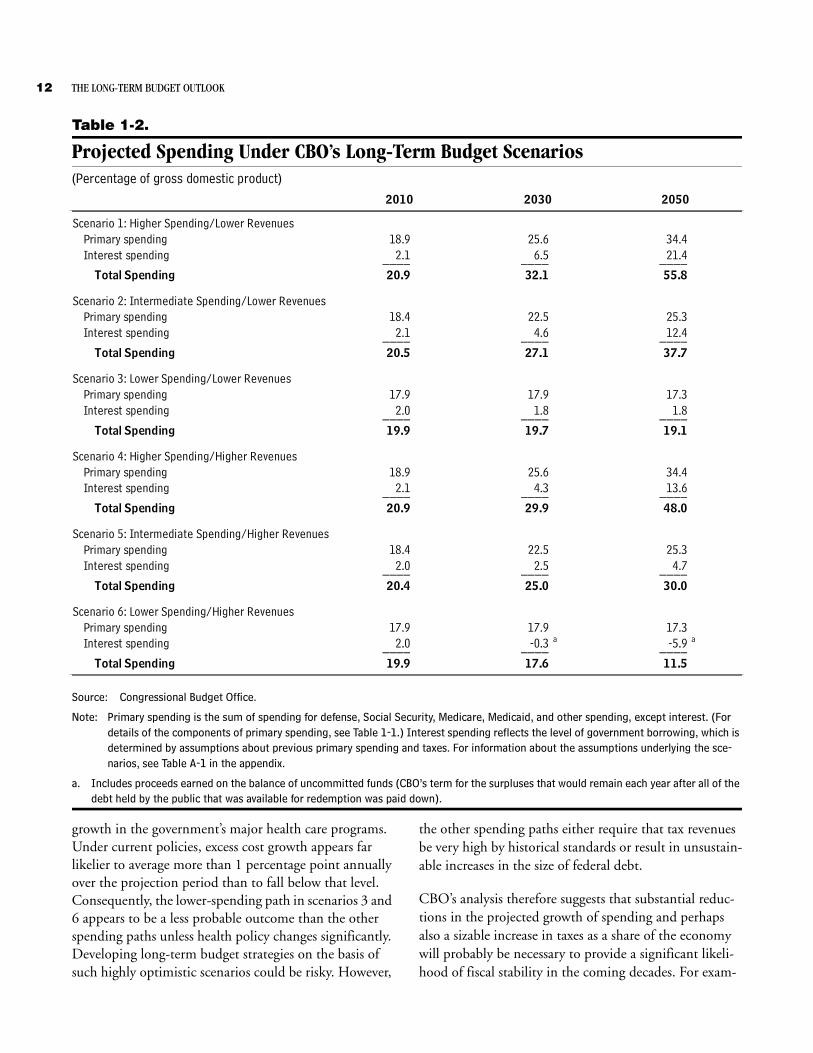
Projected Spending Under CBO’s Long-Term Budget Scenarios (Percentage of gross domestic product)
Source: Congressional Budget Office.
Note: Primary spending is the sum of spending for defense, Social Security, Medicare, Medicaid, and other spending, except interest. (For details of the components of primary spending, see Table 1-1.) Interest spending reflects the level of government borrowing, which is determined by assumptions about previous primary spending and taxes. For information about the assumptions underlying the sce-narios, see Table A-1 in the appendix.
a. Includes proceeds earned on the balance of uncommitted funds (CBO’s term for the surpluses that would remain each year after all of the debt held by the public that was available for redemption was paid down).
18.9 25.6 34.42.1 6.5 21.4____ ____ ____
Total Spending 20.9 32.1 55.8
18.4 22.5 25.32.1 4.6 12.4____ ____ ____
Total Spending 20.5 27.1 37.7
17.9 17.9 17.32.0 1.8 1.8____ ____ ____
Total Spending 19.9 19.7 19.1
18.9 25.6 34.42.1 4.3 13.6____ ____ ____
Total Spending 20.9 29.9 48.0
18.4 22.5 25.32.0 2.5 4.7____ ____ ____
Total Spending 20.4 25.0 30.0
17.9 17.9 17.32.0 -0.3 a -5.9 a
____ ____ ____Total Spending 19.9 17.6 11.5
Interest spending
Primary spendingInterest spending
Scenario 6: Lower Spending/Higher RevenuesPrimary spending
Scenario 4: Higher Spending/Higher RevenuesPrimary spendingInterest spending
Scenario 5: Intermediate Spending/Higher Revenues
Interest spending
Scenario 1: Higher Spending/Lower Revenues
Scenario 2: Intermediate Spending/Lower Revenues
Scenario 3: Lower Spending/Lower Revenues
Interest spending
Primary spendingInterest spending
Primary spending
2010 2030 2050
Primary spending
growth in the government’s major health care programs. Under current policies, excess cost growth appears far likelier to average more than 1 percentage point annually over the projection period than to fall below that level. Consequently, the lower-spending path in scenarios 3 and 6 appears to be a less probable outcome than the other spending paths unless health policy changes significantly. Developing long-term budget strategies on the basis of such highly optimistic scenarios could be risky. However,
the other spending paths either require that tax revenues be very high by historical standards or result in unsustain-able increases in the size of federal debt.
CBO’s analysis therefore suggests that substantial reduc-tions in the projected growth of spending and perhaps also a sizable increase in taxes as a share of the economy will probably be necessary to provide a significant likeli-hood of fiscal stability in the coming decades. For exam-

CHAPTER ONE ECONOMIC AND FISCAL IMPLICATIONS OF FEDERAL BUDGETARY CHOICES OVER THE LONG RUN 13
ple, if spending for programs other than Social Security, Medicare, and Medicaid is tightly constrained to CBO’s hypothetical low path and if revenues are kept at their historical average of 18.3 percent of GDP, excess cost growth in Medicare and Medicaid will have to be nearly eliminated to prevent an indefinite spiraling of federal debt. Alternatively, if that other spending is constrained to the low path and if excess cost growth is held to an av-erage of 1.0 percentage point a year, revenues will have to rise continually to maintain long-term fiscal stability.
Some commonly discussed proposals to change Social Se-curity, Medicare, and Medicaid would alter the fiscal im-balances present in some of those scenarios. One example is to raise the age at which people become eligible for full Social Security retirement benefits and for Medicare to 70 by 2037. That policy would lower spending for those programs by a total of 1.6 percent of GDP by 2050.9 However, the policy would not dramatically change the ultimate path for federal debt if excess cost growth con-tinued at 1.0 percentage point or more annually.
Another policy combination—allowing initial Social Security benefits to increase at the same rate as prices rather than wages and raising Medicare’s eligibility age to 67—would restrain spending to a greater degree, reduc-ing it by 1.9 percent of GDP by 2050. Ultimately, how-ever, that restraint would not be enough to offset excess cost growth of 1.0 percentage point or more. (Those and other options to curb the growth of spending for Social Security, Medicare, and Medicaid are discussed in Chap-ters 2 and 3.)
Alternatively, tax policies might serve as a mechanism for mitigating the fiscal pressure illustrated in some of the scenarios. One crude way to gauge the effect of using tax policies for that purpose is to assume that revenues jump by 19 percent in 2007—to 20.9 percent of GDP, the highest level since World War II—and remain there per-manently. Compared with the higher-spending/lower revenue and intermediate-spending/lower-revenue sce-narios, that change would postpone adverse fiscal out-comes—but eventually, the growth of spending would cause federal debt to resume its rapidly escalating path. Compared with the higher-spending/higher-revenue sce-nario, that change would produce higher revenues over
9. That estimate excludes the effects of the policy on other federal health programs, such as Medicaid and health insurance for fed-eral civilian employees and members of the military.
the next decade or so but lower revenues thereafter, re-sulting in less debt issuance early in the projection but a much steeper rise toward the end of the 50-year period.
The Economic Effects of Growing Federal DebtThe budget scenarios described above do not incorporate the economic effects of the various spending and tax poli-cies underlying them. The remainder of this chapter ana-lyzes those effects and draws the following conclusions:
B A budget policy that caused federal debt to grow con-tinually faster than GDP could seriously harm the economy. Rising government debt can sap national saving, slow private capital formation, lower economic growth, and in the extreme, produce a sustained eco-nomic contraction. Moreover, such a policy could increase the United States’ indebtedness to other nations, implying that more of the economy’s output would have to be used to pay interest on the debt and less would be available for U.S. residents.
B The nation is unlikely to be able to grow its way out of the sorts of long-term budgetary problems that would result under the scenarios that entail high levels of fed-eral debt.
B Decisions about how to resolve the nation’s long-term budgetary challenges will have economic implications. For example, sharply raising marginal tax rates could have a detrimental effect on incentives for people to work and save—and thus on the size of the econ-omy—whereas reducing the growth of spending could lessen those negative effects.10
B Impacts on the economy are not the only criteria for evaluating government policies. Considerations such as fairness and well-being are also relevant. Evaluating those other effects, however, is beyond the scope of this report.
B If changes were made to programs for the elderly, announcing those changes far in advance could give people time to adjust their plans for work and sav-ing—and thus could lessen the overall cost of the changes.
10. Marginal tax rates are the rates that people pay on an additional dollar of income.

14 THE LONG-TERM BUDGET OUTLOOK
How Would Rising Debt Affect the Economy?Some of the scenarios described above would push federal debt held by the public to unsustainable levels. For exam-ple, if the excess growth of health care costs per enrollee declined to 1.0 percentage point in the long run and rev-enues averaged 18.3 percent of GDP (scenario 2, the intermediate-spending/lower-revenue scenario), the annual budget deficit would climb from 2.6 percent of GDP in 2005 to 19 percent by 2050, CBO projects. In that scenario, persistent and growing deficits eventually push the total amount of federal debt to unprecedented levels: from 38 percent of GDP in 2005 to about 256 percent in 2050 and rapidly rising levels thereafter. The outcomes in the higher-spending scenarios (1 and 4) would be even more dramatic.
In each of those scenarios, the growth of debt would accelerate as the government attempted to finance its interest payments by issuing more debt—leading to a vicious circle in which ever-larger amounts of debt were issued to pay ever-higher interest charges. Eventually, the costs of servicing the debt would outstrip the govern-ment’s ability to pay them, thus becoming unsustainable.
However, as noted in Box 1-1, budget deficits are not always harmful. When the economy is in a recession, def-icits can stimulate demand for goods and services and bring resources back to full employment. They can also provide critical financing during wartime.11 But the defi-cits in CBO’s long-term scenarios occur not because the government is trying to pull the economy out of a reces-sion or fight a war, but because it is spending more and more on programs for the elderly and on interest pay-ments on accumulated debt.
Impact on Capital, Productivity, and Growth. Sustained and rising budget deficits would affect the economy by absorbing funds from the nation’s pool of savings and reducing investment in both the domestic capital stock and foreign assets.12 Investment in business structures, equipment, research and development, worker training,
11. In principle, deficits could also be used to finance productive long-term government investments, although it is difficult to define and identify what constitutes a productive investment. A review of the economics literature suggests that many federal investment projects yield small, or even negative, net benefits for the economy. See Congressional Budget Office, The Economic Effects of Federal Spending on Infrastructure and Other Investments (June 1998).
and education would be lower than it would be in the absence of such large levels of federal borrowing. As a result, the growth of workers’ productivity would gradu-ally slow, real wages would begin to stagnate, and eco-nomic growth would tend to taper off. If that situation continued long enough, rising deficits could actually lead to a sustained contraction of the economy. Although some portion of the deficit could be financed by foreign investors—lessening the degree to which the deficit crowded out investment in the domestic capital stock—borrowing from abroad would not be free. Over time, foreign investors would claim larger shares of the nation’s output. In the end, fewer resources would be available for domestic consumption.
Taken to the extreme, such a path could result in an eco-nomic crisis. Foreign investors could reduce their pur-chases of U.S. securities, the exchange value of the dollar could plunge, interest rates could climb, consumer prices could shoot up, or the economy could contract sharply. Amid the anticipation of declining profits and rising inflation and interest rates, stock markets could collapse and consumers might sharply reduce their consumption. Moreover, economic problems in the United States could spill over to the rest of the world and seriously weaken the economies of U.S. trading partners.
A policy of higher inflation could reduce the real value of the government’s debt, but inflation is not a feasible long-term strategy for dealing with persistent budgetdeficits. To be sure, unexpected increases in inflation would enable the government to repay its debts in cheaper dollars and make borrowers better off at the expense of creditors. But financial markets would not be fooled forever; investors would eventually demand higher interest rates. If the government continued to print money to finance the deficit, the situation would eventu-ally lead to hyperinflation (as happened in Germany in the 1920s, Hungary in the 1940s, Argentina in the 1980s, and Yugoslavia in the 1990s). Moreover, interest
12. That situation would arise unless the private sector responded by increasing its saving by the amount of the deficit; see Robert Barro, “Are Government Bonds Net Wealth?” Journal of Political Economy, vol. 82, no. 6 (November/December 1974), pp. 1095- 1117. Such a response would be at odds with empirical evidence, however. See Paul Evans, “Consumers Are Not Ricardian: Evi-dence from Nineteen Countries,” Economic Inquiry, vol. 31, no. 4 (October 1993), pp. 534-548; and T.D. Stanley, “New Wine in Old Bottles: A Meta-Analysis of Ricardian Equivalence,” Southern Economic Journal, vol. 64, no. 3 (January 1998), pp. 713-727.

CHAPTER ONE ECONOMIC AND FISCAL IMPLICATIONS OF FEDERAL BUDGETARY CHOICES OVER THE LONG RUN 15
rates could remain high for some time even after inflation was brought back under control. Once a government has lost credibility in financial markets, regaining it can be difficult. In the end, inflationary financing cannot ad-dress the fundamental problem that spending exceeds revenues.
Faster economic growth could improve the budget out-look, but such growth on its own is unlikely to solve the budgetary problems that the nation would face in the high-debt scenarios.13 Although faster growth would push up revenues in the near term, it would also raise spending later on. Social Security benefits, for example, depend on each worker’s wage history, so gains in real wages would automatically translate into higher benefits in the long term. Indeed, a recent CBO analysis con-cluded that there was virtually no chance that higher pro-ductivity growth (which is a major driver of the growth of the economy in the long run) could by itself resolve the financial imbalances in the Social Security program.14 Moreover, if the past is any guide, federal health care spending would also rise with an expanding economy. For all of those reasons, faster economic growth could provide only temporary relief in the high-debt scenarios.
Is There a Safe Level of Debt? Budgetary paths are eco-nomically unsustainable not when federal debt hits a crit-ical level but when the government adopts policies that cannot be carried out indefinitely. Because future policies are what matter, no bright line separates safe from unsafe levels of debt. However, the projected debt in some of CBO’s scenarios is large by any standard. Since the founding of the United States, the annual budget deficit has exceeded 10 percent of GDP in only a few instances, during major wars. Moreover, total federal debt held by the public has surpassed 100 percent of GDP just once—for a brief period during World War II (see Figure 1-3).
13. Several analysts have examined the effects of alternative economic assumptions on the long-term budget outlook. See Congressional Budget Office, Quantifying Uncertainty in the Analysis of Long-Term Social Security Projections (November 2005); and Social Security Administration, The 2005 Annual Report of the Board of Trustees of the Federal Old-Age and Survivors Insurance and Disabil-ity Insurance Trust Funds (March 23, 2005).
14. Statement of Douglas Holtz-Eakin, Director, Congressional Bud-get Office, The Role of the Economy in the Outlook for Social Secu-rity, before the Subcommittee on Social Security, House Committee on Ways and Means, June 21, 2005; and Congres-sional Budget Office, Quantifying Uncertainty in the Analysis of Long-Term Social Security Projections, Table 8.
That budgetary situation was temporary, however; as soon as the war was over, federal debt held by the public began to decline as a share of the economy. In fact, until the 1980s, the ratio of debt to GDP had never risen sig-nificantly during a period of peace and prosperity, as it would under several of CBO’s long-term scenarios (see Figure 1-2 on page 11).
Other nations have accumulated high levels of debt. For example, during the second half of the 1990s, net public debt averaged about 106 percent of GDP in Italy and 118 percent in Belgium.15 Unlike the projections of debt in CBO’s scenarios, however, those countries’ experience involved debts that increased and then remained fairly stable relative to GDP, not debts that rose ever faster. Even so, to keep their debts under control, those govern-ments had to run large primary surpluses (in which reve-nues exceeded noninterest spending) simply to cover their interest payments.
How Would Alternative Budgetary StrategiesAffect the Economy?The goods and services that baby boomers will consume in their retirement will be produced largely by the econ-omy when they are retired. Thus, the bigger the econ-omy, the easier it will be for the nation to adjust to an aging population.
Moving the budget off an unsustainable track would pro-vide significant economic benefits to the U.S. economy in the long run by reducing the economic risks discussed above. However, the budget could be put on a sustainable track in various ways, and different budgetary strate-gies—such as lowering the growth of benefit payments to the elderly or raising taxes—could have different effects on the economy.
Slowing the growth of spending by reducing future retir-ees’ benefits, for example, could be one way to lessen the future pressures on the budget and expand the economy. Such a policy would probably encourage saving and in-crease the capital stock, although the size of the effect—and its path over time—is very uncertain. The results would depend on the extent to which workers anticipated and responded to the cuts in their future benefits. Forward-looking workers would probably reduce their current consumption and increase their saving in the
15. Organisation for Economic Co-operation and Development, Eco-nomic Outlook (Paris: OECD, June 2005).

16 THE LONG-TERM BUDGET OUTLOOK
Figure 1-3.
Federal Debt Held by the Public as a Percentage of GDP, 1790 to 2004
Source: Congressional Budget Office using data on federal debt from the Department of the Treasury and the Board of Governors of the Fed-eral Reserve System. Estimates of gross domestic product (GDP) come from the Bureau of the Census; Thomas Berry, Revised Annual Estimates of American Gross National Product (Richmond, Va.: Bostwick Press, 1978); Robert E. Gallman, “Economic Growth and Structural Change in the Long Nineteenth Century,” in Gallman and Stanley L. Engerman, eds., The Cambridge Eco-nomic History of the United States, vol. 2, The Long Nineteenth Century (Cambridge, England: Cambridge University Press, 2000), pp. 1-55; Nathan S. Balke and Robert J. Gordon, “The Estimation of Prewar Gross National Product: Methodology and New Evi-dence,” Journal of Political Economy, vol. 97, no. 1 (February 1989), pp. 38-92; and the Department of Commerce, Bureau of Eco-nomic Analysis.
1790 1805 1820 1835 1850 1865 1880 1895 1910 1925 1940 1955 1970 1985 20000
20
40
60
80
100
120
expectation of receiving smaller benefits. However, some people might not be so foresighted. They might not reduce their consumption until retirement, when they received smaller benefit checks.
Slowing the growth of future payments to the elderly might also affect the supply of labor. That effect, too, is uncertain and would depend on the nature of the policy changes. Some reductions in future benefits could encourage people to work more to make up for the lost income; other types of reductions might discourage work by reducing the marginal return from an additional hour of work.
Policymakers could also raise taxes to alleviate future pres-sure on the budget, although the economic effects of that policy would depend on the type of tax that was raised. All else being equal, tax policies that increase marginal tax rates may reduce people’s incentives to work and save,
distort their economic decisions, and increase inefficien-cies in the economy.16 Moreover, those inefficiencies tend to grow disproportionately with the tax rate. Economic distortions are smaller when revenues are raised through changes in tax policies that have smaller effects on mar-ginal incentives to work and save. Examples of such pol-icy changes include reductions in the child tax credit, per-sonal exemptions, and standard deductions.
Illustrative Simulations of Alternative Budgetary Strate-gies. CBO used a model of economic growth to illumi-nate the character of the economic effects of those alter-native budgetary strategies. The model was selected because it distinguishes between people born in different years, making it well suited to analyze the impacts of pro-
16. See Congressional Budget Office, Effective Marginal Tax Rates on Labor Income (November 2005), Corporate Income Tax Rates: International Comparisons (November 2005), and Labor Supply and Taxes (January 1996).

CHAPTER ONE ECONOMIC AND FISCAL IMPLICATIONS OF FEDERAL BUDGETARY CHOICES OVER THE LONG RUN 17
grams such as Social Security and Medicare.17 The model incorporates the assumption that people are forward- looking and will adjust their behavior in anticipation of future changes in tax rates and benefits.
CBO used the model to compare the effects of two alter-native budget policies. Both policies are sustainable, but they have different implications for the economy. The first policy permits revenues to rise as much as in the higher-revenue (current-law) path presented earlier and uses the additional revenues to finance higher spending on programs for the elderly. Under that policy, marginal tax rates rise gradually because real income growth pushes people into higher tax brackets and makes them subject to the alternative minimum tax. The effective marginal tax rate on labor income increases from 30.6 percent in 2006 to 38.2 percent in 2050, and the effective marginal rate on capital income increases from 15.3 percent in 2006 to about 16.5 percent in 2050.18 As a result, total federal revenues as a share of GDP grow by 6.2 percent-age points between 2006 and 2050 (before considering economic feedbacks). Because that simulation incorpo-rates the assumption that additional revenues are spent on retirement-related programs, spending as a share of GDP also increases by 6.2 percentage points over the same period.19 By design, the policy is meant to be sus-tainable over the long term.
The alternative policy is also sustainable but focuses on a lower-tax, lower-spending strategy. Specifically, the policy keeps revenues constant as a share of GDP and eliminates the rise in spending on programs for the elderly that occurs under the first policy.
Both policies would alter the flow of savings to domestic capital markets, international capital markets, or both. To illustrate the importance of international capital markets, the model uses two different assumptions—polar oppo-sites—about the degree of openness of the economy. The
17. For more information about the model, see Congressional Budget Office, How CBO Analyzed the Macroeconomic Effects of the Presi-dent’s Budget (July 2003); and Shinichi Nishiyama, Analyzing an Aging Population—A Dynamic General Equilibrium Approach, CBO Technical Paper 2004-03 (February 2004).
18. Those estimates include payroll taxes and federal and state indi-vidual income taxes.
19. The growth of noninterest spending under that policy is slightly lower than it is in the intermediate-spending path described earlier.
first posits a closed economy, in which domestic markets are insulated from the rest of the world, and thus, interest rates and wage rates are determined solely by domestic forces. The second alternative is a small open economy; in that case, interest rates and wages are fixed by world markets. In actuality, the U.S. economy is somewhere between those two extremes.
The simulations suggest that policies with higher mar-ginal tax rates and higher spending on programs for the elderly tend to produce weaker economic growth than do policies that entail lower marginal tax rates and lower spending on such programs. In the closed-economy ver-sion of the model, real GDP under the higher-tax, higher-spending policy is about 6 percent lower in 2050 than it is under the lower-tax, lower-spending policy.20 That result stems from the fact that higher marginal tax rates on labor discourage work, and higher spending on retirement-related programs reduces incentives for people to save for retirement. Under the higher-tax, higher- spending policy, the labor supply is about 3 percent smaller and the capital stock about 13 percent smaller in 2050 than under the alternative policy. That pattern of results is generally consistent with those of other models.
By comparison, the open-economy version of the model produces smaller effects on real GDP. In the simulation, real GDP is only 2 percent lower in 2050 under the higher-tax, higher-spending policy than under the lower- tax, lower-spending policy. That difference is narrower because capital inflows from abroad mute the impact of lower domestic saving on the capital stock. As a result, the capital stock declines by only 2 percent by 2050. However, because a larger fraction of GDP must be used to service U.S. debt to foreigners, real gross national product (which measures national income after deduct-ing net payments to foreigners) falls by 7 percent by 2050.
Those changes are significant—7 percent of gross national product in today’s economy is more than three-quarters of a trillion dollars—but they are small com-pared with the economic benefits of moving the budget onto a sustainable track. Both of the policy alternatives considered in this section are sustainable in the sense that they would prevent government debt from growing
20. If the level of real GDP is about 6 percent lower in 2050, the aver-age annual growth rate of real GDP between 2006 and 2050 is 0.13 percentage points smaller than it would be otherwise.

18 THE LONG-TERM BUDGET OUTLOOK
explosively. Such sustainable policies could provide a pol-icy environment under which the economy could con-tinue to grow. If workers’ productivity kept advancing as it has in the past, real GDP could double or triple over the next 50 years, CBO projects. If, by contrast, the bud-get remained on an unsustainable track, the nation would face rising risks that the growth of workers’ productivity could falter and economic growth could deteriorate.
The Costs of Delay. Because interest costs rise as debt grows, the longer that policymakers delay acting to counter an unsustainable budgetary situation, the larger the spending cuts or tax increases will eventually have to be. Delay also raises another problem: as interest costs
mount, the government’s flexibility to deal with unex-pected developments, such as a war or a recession, diminishes.
Delay can also impose costs on households. The longer that action is put off, the greater the chance that policy changes will occur suddenly, making it difficult for households to react. Thus, announcing changes in popu-lar entitlement programs or in the tax structure well be-fore they take place can give people time to adjust their plans for saving and retirement. Those adjustments can significantly lessen the costs of making the policy changes and reduce the impact on workers’ and retirees’ standards of living.

C HA P T E R
2The Long-Term Outlook for Social Security
Chapter 2: The Long-Term Outlook for Social Security
Social Security is by far the federal government’s largest income-redistribution program. The program consists of two parts: Old-Age and Survivors Insurance pays benefits to retired workers and to their dependents and survivors; and Disability Insurance (DI) makes pay-ments to disabled workers who are younger than the nor-mal retirement age and to their dependents. In all, about 48 million people now receive Social Security benefits.1
Driven largely by repeated expansions of the program during its first 40 years, spending for Social Security ben-efits steadily increased relative to the size of the economy, reaching 4 percent of gross domestic product in 1975 (see Figure 2-1). Since then, that spending has generally fluc-tuated between 4.0 percent and 4.5 percent of GDP. In 2005, it accounted for an estimated 4.2 percent of GDP.
The Outlook for Social SecuritySpendingThe cost of the Social Security program will rise signifi-cantly in coming decades—a change that has long been foreseen. Average benefits typically grow when the econ-omy does (because the earnings on which those benefits are based increase). However, in the future, the total amount of Social Security benefits paid will grow faster than the overall economy because of changes in the
1. The projections presented here differ somewhat from those included in the Congressional Budget Office’s December 2003 Long-Term Budget Outlook, which were based primarily on inter-mediate projections in Social Security Administration, The 2003 Annual Report of the Board of Trustees of the Federal Old-Age and Survivors Insurance and Disability Insurance Trust Funds (March 17, 2003). For details on CBO’s current Social Security projection methodology, see The Outlook for Social Security (June 2004). For a more general discussion of how the Social Security program works and how changes to it might affect the nation’s ability to deal with impending demographic shifts, see Congressional Bud-get Office, Social Security: A Primer (September 2001).
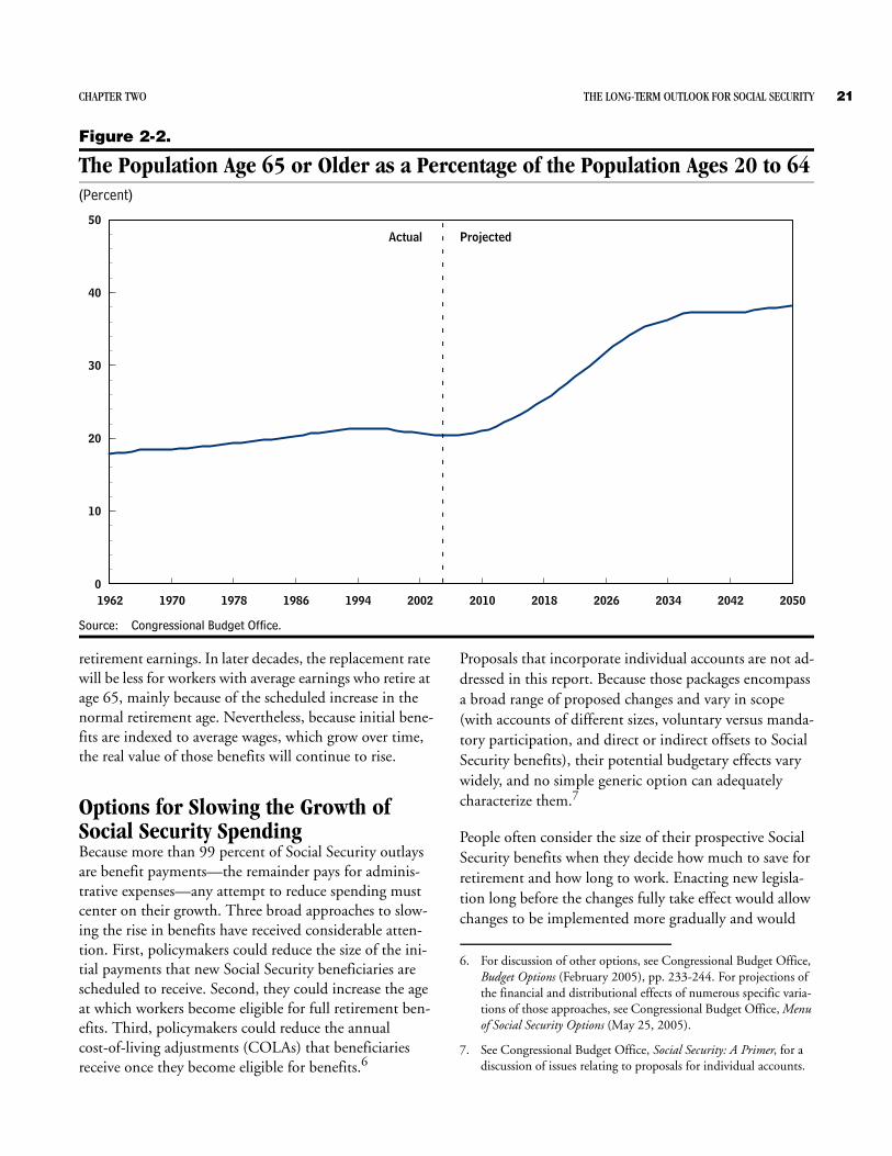
nation’s demographic structure. As the baby-boom gener-ation reaches retirement age, and as decreasing mortality leads to longer lives and longer retirements, a larger share of the population will draw Social Security benefits.2 Moreover, whereas the number of adults under age 65 is projected to grow by 12 percent in the next 30 years, the number of people age 65 or older is projected to double. As a result, in three decades, the older population is likely to be more than one-third the size of the younger group, compared with one-fifth today (see Figure 2-2). Con-sequently, the Congressional Budget Office estimates that unless changes are made to Social Security, spending for the program will rise to 5.0 percent of GDP in 2020, 6.0 percent in 2030, and 6.4 percent in 2050.
Discussions of Social Security frequently address the sta-tus of the program’s trust funds. However, this chapter considers total scheduled Social Security outlays, which if paid would require substantial resources.3 (Revenues, the means of providing such resources, are examined in Chapter 5 of this report.)
How Social Security FunctionsIn general, workers are eligible for retirement benefits if they are age 62 or older and have paid sufficient Social Security taxes for at least 10 years. Workers whose em-
2. For a summary of the retirement prospects of the baby-boom generation, see Congressional Budget Office, The Retirement Prospects of the Baby Boomers (March 18, 2004); for details, see Congressional Budget Office, Baby Boomers’ Retirement Prospects: An Overview (November 2003).
3. Analyses of Social Security may distinguish between benefits as scheduled and the benefits that would be legally payable under current law (which could be lower than scheduled benefits if the Social Security trust funds were exhausted). That distinction is not important, however, for this report. CBO projects that the Social Security trust funds will remain solvent through 2050, so during that period, scheduled benefits are identical to current-law benefits.

20 THE LONG-TERM BUDGET OUTLOOK
Figure 2-1.
Spending for Social Security, 1962 to 2050(Percentage of gross domestic product)
Source: Congressional Budget Office.
1962 1970 1978 1986 1994 2002 2010 2018 2026 2034 2042 20500
1
2
3
4
5
6
7Actual Projected
ployment has been limited because of a physical or men-tal disability can become eligible for DI benefits at an ear-lier age and often with a shorter employment history.
When retired or disabled workers first claim Social Secu-rity benefits, they receive payments based on their average earnings over their working lifetime; those payments are subsequently adjusted to reflect annual changes in con-sumer prices. The formula used to translate average earn-ings into benefits is progressive—in other words, it re-places a larger share of preretirement earnings for people with lower average earnings than it does for people with higher earnings. Both the earnings history and the spe-cific dollar amounts included in the formula are indexed for changes in average annual earnings for the labor force as a whole.4 Because average national earnings generally grow in real terms (faster than the rate of inflation), that indexation causes initial benefits for future recipients to grow in real terms.
4. For a more detailed description of that formula, see Congressional Budget Office, Social Security: A Primer, Chapter 2.
For retirement benefits, a final adjustment is made on the basis of the age at which the recipient chooses to start claiming benefits—the longer a person waits (up to age 70), the higher the benefits will be. That final adjustment is intended to be “actuarially fair,” so that an individual’s total lifetime benefits will be approximately equally valu-able regardless of when he or she begins collecting them.
For workers born before 1938, the age of eligibility for full retirement benefits—referred to as Social Security’s “normal retirement age”—was 65. Under current law, that age is gradually increasing and will be 67 for people born in 1960 or later.5 Workers will still be able to choose to begin receiving reduced benefits as early as age 62.
People who turn 65 over the next decade will, on average, receive annual retirement benefits of about $14,000 (in 2005 dollars) if they claim benefits at age 65. That amount will replace about 45 percent of their pre-
5. Specifically, the normal retirement age rises by two months per birth year for people born from 1938 through 1943 and again by two months per year for people born from 1955 through 1960.
CHAPTER TWO THE LONG-TERM OUTLOOK FOR SOCIAL SECURITY 21
Figure 2-2.
The Population Age 65 or Older as a Percentage of the Population Ages 20 to 64(Percent)
Source: Congressional Budget Office.
1962 1970 1978 1986 1994 2002 2010 2018 2026 2034 2042 20500
10
20
30
40
50Actual Projected
retirement earnings. In later decades, the replacement rate will be less for workers with average earnings who retire at age 65, mainly because of the scheduled increase in the normal retirement age. Nevertheless, because initial bene-fits are indexed to average wages, which grow over time, the real value of those benefits will continue to rise.
Options for Slowing the Growth of Social Security SpendingBecause more than 99 percent of Social Security outlays are benefit payments—the remainder pays for adminis-trative expenses—any attempt to reduce spending must center on their growth. Three broad approaches to slow-ing the rise in benefits have received considerable atten-tion. First, policymakers could reduce the size of the ini-tial payments that new Social Security beneficiaries are scheduled to receive. Second, they could increase the age at which workers become eligible for full retirement ben-efits. Third, policymakers could reduce the annual cost-of-living adjustments (COLAs) that beneficiaries receive once they become eligible for benefits.6
Proposals that incorporate individual accounts are not ad-dressed in this report. Because those packages encompass a broad range of proposed changes and vary in scope (with accounts of different sizes, voluntary versus manda-tory participation, and direct or indirect offsets to Social Security benefits), their potential budgetary effects vary widely, and no simple generic option can adequately characterize them.7
People often consider the size of their prospective Social Security benefits when they decide how much to save for retirement and how long to work. Enacting new legisla-tion long before the changes fully take effect would allow changes to be implemented more gradually and would
6. For discussion of other options, see Congressional Budget Office, Budget Options (February 2005), pp. 233-244. For projections of the financial and distributional effects of numerous specific varia-tions of those approaches, see Congressional Budget Office, Menu of Social Security Options (May 25, 2005).
7. See Congressional Budget Office, Social Security: A Primer, for a discussion of issues relating to proposals for individual accounts.

22 THE LONG-TERM BUDGET OUTLOOK
give people more time to plan for and adjust to the changes.
The rest of this chapter looks at specific ways to imple-ment the three broad approaches described above. The estimates of savings are intended to indicate the relative magnitudes of alternative changes; specific estimates of savings would depend on the details of individualproposals.
Option 1: Constrain the Increase in Initial Benefits A straightforward way to reduce the growth of Social Se-curity spending would be to slow the rate at which initial benefits rise from one cohort of recipients to the next. Each new group of eligible beneficiaries would then re-ceive lower benefits than scheduled under current law. However, that approach would not alter the benefits of people already on the rolls before the change took effect.
One method that has received considerable attention would be to change the way initial benefits are calculated so that they grow with prices instead of wages. The bene-fits awarded to each succeeding cohort would still rise in nominal terms, but only by enough to keep up with infla-tion. The effect of this change on benefits can be de-scribed in several ways:8
B In real terms, annual benefits would be unchanged. Future retirees would have the same purchasing power that retirees have today, under an assumption that all retirees claimed benefits at the normal retirement age.
B Measured over a lifetime, total benefits would still in-crease because longevity is expected to keep growing.
B Compared with wages, annual benefits would fall (in other words, the replacement rate would decline).
B Compared with the amounts that future beneficiaries are scheduled to receive under current law, benefits would fall.
The decline relative to currently scheduled benefits would grow larger for each future cohort of retirees. Under the specific option modeled here, initial benefits would grow with prices for people turning 62 in 2013 or later. If real
8. See Congressional Budget Office, Measuring Changes to Social Security Benefits, Long-Range Fiscal Policy Brief No. 11(December 1, 2003).
wages grew at an average rate of 1.3 percent per year, as this analysis assumes, workers who became eligible for benefits in 2030 would receive 21 percent less under this option than they are scheduled to under current rules. Workers who became eligible in 2050 would receive about 39 percent less.
Adopting this option would reduce outlays for Social Security in 2050 by about 26 percent from the level pro-jected under current law. As a result, those outlays would equal 4.7 percent of GDP instead of 6.4 percent (see Figure 2-3). Thereafter, Social Security spending would continue to decline as a share of GDP.
For simplicity, this illustrative option would result in the same percentage change in benefit levels for all beneficia-ries in a cohort. However, a comprehensive policy pro-posal could include other adjustments that would protect certain beneficiaries from the proposed changes—for ex-ample, by setting a minimum benefit level or by making the existing benefit formula more progressive.
Option 2: Raise the Retirement AgeFor retirees, increasing the normal retirement age would be equivalent to reducing annual benefit levels. Since benefit levels are designed to be actuarially fair regardless of the age at which someone begins receiving benefits, changing the early-retirement age from 62 would have relatively little effect on total Social Security spending, al-though it might induce people to work longer and there-fore pay more payroll taxes. By contrast, raising the nor-mal retirement age would result in lower spending. If retirees responded by claiming benefits later, they would receive the same annual benefits but for fewer years. If they did not change the age at which they claimed bene-fits, they would receive reduced annual benefits for the same length of time.
Some Members of Congress and others have recom-mended accelerating the current shift to a normal retire-ment age of 67 and raising that age further thereafter. Proponents of such a change point out that when Social Security benefits were first paid in 1940, the life expect-ancy of 65-year-olds was about 13 years. Today, it is about 18 years, and life expectancy is expected to con-tinue to grow.
Debate about the level of Social Security benefits tends to focus on how much people will receive each month rather than on how much they will receive over their lifetimes.

CHAPTER TWO THE LONG-TERM OUTLOOK FOR SOCIAL SECURITY 23
Figure 2-3.
Federal Spending Under Current Law and Under Three Illustrative Options for Slowing the Growth of Social Security(Percentage of gross domestic product)
Source: Congressional Budget Office.
Note: COLAs = cost-of-living adjustments.
2005 2010 2015 2020 2025 2030 2035 2040 2045 20500
3
4
5
6
7
Current Law
Option 2 :Raise the
Retirement AgeFurther
Option 3:Reduce COLAs Option 1:
Constrain theIncrease in
Initial Benefits
But because of increasing longevity, a commitment to give retired workers a certain amount of monthly benefits at age 62 in, say, 2030 is likely to be more expensive over the recipients’ lifetimes than that same commitment made to retirees today. The swell of the baby-boom gen-eration will cause most of the growth in the number of Social Security beneficiaries over the next 30 years. But in the longer term, the growth in the number of ben-eficiaries—and in costs—will be driven by projected in-creases in longevity. Linking the normal retirement age to future increases in life expectancy is one way of dealing with that source of cost growth.
The specific option considered here (illustrated in Table 2-1) would speed the transition to a normal retire-ment age of 67 and then raise that age further to keep pace with assumed future increases in life expectancy. For workers born in 1949, the normal retirement age would be 67. Thereafter, the retirement age would increase by two months per year until it reached 70 for people born in 1967. After that, it would rise by one month every other year. As under current law, workers would still be
able to receive reduced benefits starting at age 62, but the corresponding reduction in benefits would be more significant.
This option would produce substantial savings relative to spending levels scheduled under current law: by 2050, the savings would be about 12 percent. Outlays would be 5.6 percent of GDP instead of 6.4 percent in that year and would continue to decline slightly as a share of GDP thereafter.
This option would not affect the scheduled benefits of workers who qualified for Disability Insurance. Thus, as DI benefits became relatively more attractive, older work-ers nearing retirement would be more likely to apply for them. To avoid strengthening that incentive, policy-makers could make similar adjustments to scheduled DI benefits—for example, by linking the benefits for workers who qualified for DI to the amount those workers would have received if they had retired at a specific age, such as 65 or 67. (Under current law, their benefits are linked to

24 THE LONG-TERM BUDGET OUTLOOK
Table 2-1.
The Increase in Social Security’s Normal Retirement Age Under Current Law and Under an Illustrative Option
Source: Congressional Budget Office based on data from the Social Security Administration, Office of the Actuary.
a. Under this option, the normal retirement age would reach 67 for workers born in 1949. The retirement age would increase by two months for each birth year thereafter until it reached 70 for people born in 1967; it would then increase by one month for every two years.
Year of Worker'sBirth
1943 2008 66 25 71960 2025 67 30 13
1943 2008 66 25 71949 2014 67 30 131955 2020 68 35 201961 2026 69 40 251967 2032 70 45 301991 2056 71 50 35
Under Current Law
Under Illustrative Optiona
for Early Retirementin Benefits
Percentage Reduction
Year Worker Turns
Age 65
Social Security’sNormal
Retirement AgeRetirementat Age 65
Retirementat Age 62
the amount they would have received if they had retired at the normal retirement age.)
Current projections of Social Security outlays are sensi-tive to projections of life expectancy. If future beneficia-ries live longer than expected, government outlays will be higher than anticipated. A variation of this option would link the increase in the normal retirement age to actual increases in life expectancy so that total lifetime benefits would no longer grow as a result of increases in longevity, even if those increases differed from current projections.
Option 3: Reduce Cost-of-Living AdjustmentsEach year, the Social Security Administration makes a cost-of-living adjustment to monthly benefits, raising them by the percentage increase in the consumer price in-dex for urban wage earners and clerical workers (CPI-W). Since 1996, when the Advisory Commission to Study the Consumer Price Index (known as the Boskin Commis-sion) concluded that the CPI probably overstated the change in the cost of living, the Bureau of Labor Statistics (BLS) has modified the way in which it calculates the CPI several times, eliminating most of the problems identified with the index. Still, some issues remain. Most important, when the price of one good increases faster
than prices do in general, consumers buy less of that good and purchase other products instead. Because BLS bases the index on past spending patterns (currently those from 2001 and 2002), the CPI does not fully account for that “substitution effect.” On the basis of research from BLS, CBO estimates that the use of outdated spending pat-terns increases the measured annual increase in the CPI-W by about 0.3 percentage points.
A separate issue is whether the cost of living for Social Se-curity beneficiaries grows at the same rate as costs for the general population. For example, retired beneficiaries are likely to spend more than younger people on medical care, the price of which generally increases faster than the overall price level. A preliminary CPI for the elderly (CPI-E) created by BLS aims to track inflation for the population ages 62 and older. From 1983 through Sep-tember 2005, the CPI-E grew an average of 0.3 percent-age points faster than the CPI-W. That difference was attributable mostly to costs for medical care, which rose 2.6 percentage points faster than did the CPI-W.
Some policymakers suggest that Social Security law be changed to provide for a lower COLA—one equal to the annual increase in the CPI minus a specified number of

CHAPTER TWO THE LONG-TERM OUTLOOK FOR SOCIAL SECURITY 25
percentage points. If in fact the CPI still overstates in-creases in the cost of living for Social Security recipients, policymakers can reduce the COLA by an appropriate amount without making benefits any lower in real terms than they were when the recipients became eligible for them. However, if the CPI accurately measures increases in the cost of living, a reduction in the COLA will result in each beneficiary’s experiencing an annual decline in real benefits. And if the CPI currently understates the change in the cost of living for Social Security recipients, then the decline in real benefits will be made even greater.
The effects of such a change would differ from the impact of an across-the-board constraint on the increase in initial benefits (or an equivalent rise in the normal retirement age) in two ways. First, limiting the increase in initial benefits would have a progressively larger effect on each cohort. The impact on the baby-boom generation would be small, and current beneficiaries would not be affected. Reducing the COLA, by contrast, would affect all benefi-ciaries to some extent, and the benefits of all future co-horts would be reduced by roughly the same percentage. Second, the effect of a lower COLA would accumulate
each year that a participant collected benefits, so the change would generally have the largest impact on people who collected Social Security benefits the longest.
If the COLA was set to equal the increase in the CPI mi-nus 0.3 percentage points beginning in December 2006, by 2050 Social Security outlays would be about 4 percent lower than the amount projected under current law. Most of that reduction (in percentage terms) would be achieved by 2030. For example, outlays in 2030 would be 5.8 per-cent of GDP instead of 6.0 percent. Unlike in the previ-ous two options, however, spending would continue to grow as a percentage of GDP in later years.
Alternatively, lawmakers might choose to reduce cost-of-living adjustments only for Social Security recipients whose benefits or income was above specified levels; how-ever, doing that would lessen the savings. (Some benefi-ciaries with low income and few assets would receive Sup-plemental Security Income benefits, which would offset some or all of the reduction in their Social Security bene-fits. The estimate above does not account for that offset, which would slightly reduce the amount of savings.)

C HA P T E R
3The Long-Term Outlook for
Medicare and MedicaidChapter 3: The Long-Term Outlook for Medicare and Medicaid
Federal spending for Medicare and Medicaid—the two primary government-financed health care pro-grams—has been consuming a growing share of the na-tion’s economic output for decades, rising from 1.0 per-cent of gross domestic product in 1970 to 4.2 percent in 2005. Future spending growth for the programs will be driven by two fundamental factors: the aging of the pop-ulation and growth in per capita medical costs. The Medicare population will expand rapidly as baby boomers turn 65 and life expectancies continue to rise. Those demographic trends are also projected to increase Medicaid’s costs by boosting demand for long-term care. The main source of uncertainty in long-term projections of Medicare and Medicaid spending is how rapidly costs per beneficiary will increase relative to the growth of the economy. If the growth of those costs is similar to histori-cal levels, Medicare and Medicaid spending will increase much more rapidly than enrollment will. Substantially curtailing the growth rate of federal health care spending will require addressing the underlying pressures that push up health care costs overall.
Background on MedicareMedicare provides federal health insurance for 42 million people who are aged (about 85 percent of enrollees) or disabled or who have end-stage renal disease. Everyone who is eligible for Social Security benefits on the basis of age or disability ultimately qualifies for Medicare as well. The elderly become eligible for Medicare at age 65; the disabled become eligible 24 months after their Social Se-curity benefits start. While Social Security’s normal retire-ment age is scheduled to increase (see Chapter 2), Medi-care’s eligibility age is not set to change under current law.
Part A of Medicare, or Hospital Insurance, covers in-patient services provided by hospitals as well as skilled
nursing and hospice care. Part B, or Supplementary Med-ical Insurance, covers services provided by physicians and other practitioners, hospitals’ outpatient departments, and suppliers of medical equipment. Home health care may be covered by either Part A or Part B. The Medicare Prescription Drug, Improvement, and Modernization Act of 2003 (MMA) added a voluntary prescription drug benefit that becomes available in 2006 under a newly cre-ated Part D.
Benefits under Part A are financed primarily by current workers’ payroll taxes. Enrollees’ premiums cover 25 per-cent of the costs of the Part B program, and the rest comes from general revenues.1 Although enrollees’ premi-ums under Part D will be set at a level to cover roughly one-quarter of the cost of the basic prescription drug ben-efit, premium receipts will cover less than one-quarter of the total cost of the Part D program because certain costs of that program (such as subsidies for low-income benefi-ciaries and for employers that maintain drug coverage for their retirees) are not included in the calculation of pre-miums.
In fiscal year 2004, Medicare spending totaled an esti-mated $301.5 billion, or about $7,400 per beneficiary. About 38 percent of that spending paid for inpatient hos-pital care, and 26 percent paid for services provided by physicians and other practitioners (see Table 3-1). Ac-cording to the Congressional Budget Office’s most recent 10-year baseline projections, the new prescription drug
1. Enrollees’ premiums will cover a somewhat higher proportion of Part B costs in the future because, beginning in 2007, premiums for high-income beneficiaries will be increased. In 2007, higher premiums will be required of single enrollees with annual income over $80,000 and couples with annual income over $160,000. Those income thresholds will be indexed to inflation in future years.

28 THE LONG-TERM BUDGET OUTLOOK
Table 3-1.
Medicare Spending by Type of Service, Fiscal Year 2004
Source: Congressional Budget Office.
benefit will increase Medicare’s outlays in 2015 by about 30 percent.
Medicare beneficiaries pay part of the cost for most cov-ered services through deductibles and coinsurance. Most beneficiaries have supplemental insurance, which typi-cally pays for much of the cost sharing for Part A and Part B services and occasionally pays for some items that Medicare does not cover.
Most Medicare beneficiaries receive their care through the traditional fee-for-service (FFS) program, which pays providers for each service (or bundle of services) they pro-vide. However, 13 percent of beneficiaries receive their care through private health plans (usually health mainte-nance organizations, or HMOs) that assume financial risk and responsibility for providing Medicare benefits. A modified payment mechanism for private plans will be implemented in 2006, but it retains the essential features of the previous system. Under the modified system, plans will submit bids indicating the per capita payment for which they are willing to provide Medicare’s covered ben-efits, and the government will compare those bids with “benchmarks” that are determined through a statutory formula. Benchmarks must be at least as great as per cap-ita Medicare spending in the FFS program in every county, and in many counties they will be substantially higher than that amount. Medicare will pay plans their bids plus 75 percent of the amount by which the bench-mark exceeds their bid. Plans must return that 75 percent
113.7 3876.9 26
Suppliers’ Services39.8 1316.1 515.1 511.2 4
7.3 215.1 5
6.1 2____ ___Total 301.5 100
Administrative Expenses
Hospice ServicesOther Services
Outpatient Hospital ServicesHome Health Agency Services
Inpatient Hospital ServicesPhysicians’ and Other
Managed Care ServicesSkilled Nursing Facility Services
Percentage of Total Spending
Billions of Dollars
to their enrollees as additional benefits (such as reduced cost sharing for Medicare services) or as a rebate for their Part B or Part D premiums.2 Thus, as under the previous payment mechanism, additional benefits and premium rebates will be major incentives for enrollees to join pri-vate plans.
Background on MedicaidMedicaid is a joint federal/state program that pays for health care services for a variety of low-income individu-als. In fiscal year 2004, federal spending for the program totaled about $176 billion. Although the federal govern-ment’s share of Medicaid spending varied among states, it averaged 57 percent.
States administer their Medicaid programs under federal guidelines, which specify a minimum set of services that must be provided to certain poor residents, but eligibility and benefits vary among states. States have broad flexibil-ity and may include additional groups (such as individu-als with high medical expenses) and may provide addi-tional benefits, such as coverage for prescription drugs and dental services. By one estimate, spending on op-tional populations and benefits accounted for about 61 percent of Medicaid spending in 2001.3
By CBO’s estimates, the Medicaid program covered 57 million people in 2004, about three-quarters of whom were poor children and their parents and poor pregnant women. Per capita costs for those groups are relatively low. In contrast, expenses are higher for elderly and dis-abled beneficiaries, many of whom require long-term care. Although the elderly and disabled constitute about one-quarter of Medicaid’s enrollees, they account for 70 percent of the program’s spending (see Table 3-2). Over-all, nearly one-third of Medicaid’s spending in 2004 was for long-term care, which includes nursing home services, home health care, and other medical and social services for people whose disabilities prevent them from living in-dependently.
2. If a plan’s bid is greater than the benchmark, enrollees in that plan must pay an additional premium equal to the amount by which the plan’s bid exceeds the benchmark.
3. Henry J. Kaiser Family Foundation, Kaiser Commission on Med-icaid and the Uninsured, Medicaid Enrollment and Spending by “Mandatory” and “Optional” Eligibility and Benefit Categories (Washington, D.C.: Henry J. Kaiser Family Foundation, June 2005), p. 11.

CHAPTER THREE THE LONG-TERM OUTLOOK FOR MEDICARE AND MEDICAID 29
Table 3-2.
Distribution of Medicaid Enrollees and Benefit Payments byEligibility Category, Fiscal Year 2004(Percent)
Source: Congressional Budget Office.
Note: The numbers do not include enrollment or spending for Medicaid programs in U.S. territories.
a. Disabled enrollees include some people who are over age 65 or under age 18. Adult enrollees are adults who are not aged or disabled; they are primarily poor parents and pregnant women.
b. Long-term care includes payments for care in nursing homes and intermediate-care facilities for the mentally retarded, home health ser-vices, and other community-based services.
9.0 8.9 16.1 25.015.8 29.6 15.1 44.748.4 16.8 1.2 18.126.9 12.0 0.2 12.3_____ ____ ____ _____
Total 100.0 67.3 32.7 100.0
TotalBenefits
Distribution of Benefit Payments
BenefitsEligibility Long-Term
Care Benefitsb
Aged
CategoryaDistribution of Enrollees
Acute Care
AdultsChildrenDisabled
Medicaid covers many costs for low-income Medicare beneficiaries, including benefits that are not covered by Medicare as well as Medicare’s premiums and cost-sharing amounts. When Medicare’s prescription drug benefit takes effect in 2006, beneficiaries covered by both programs will have their prescription drug benefits cov-ered by Medicare rather than Medicaid. However, states will be required to make payments to the federal govern-ment to cover a portion of the costs they would have in-curred if they had continued to provide prescription drug benefits to beneficiaries covered by both programs. States must pay 90 percent of those estimated costs in 2006; the states’ share of those costs gradually declines to 75 per-cent by 2015, where it will remain.
In 2004, approximately 60 percent of Medicaid’s enroll-ees nationally received benefits through managed care ar-rangements, with about 40 percent enrolled in HMOs or other entities that accept responsibility and financial risk for providing a comprehensive set of Medicaid benefits.4 Another common arrangement used by states is primary care case management (PCCM), in which enrollees select (or are assigned) a primary care physician or physician group practice that assumes responsibility for overseeing
4. Centers for Medicare and Medicaid Services, “2004 Medicaid Managed Care Enrollment Report,” available at www.cms.hhs.gov/medicaid/managedcare/mmcss04.asp.
and coordinating their care. Under such arrangements, Medicaid pays providers on an FFS basis, but PCCM physicians receive an additional predetermined fee for co-ordinating their patients’ care. Some states also contract with organizations that assume responsibility and finan-cial risk for providing a subset of Medicaid benefits, such as dental services or mental health care.
Growth in the Programs’ CostsFederal costs for Medicare and Medicaid have grown faster than the economy for decades.
MedicareFrom 1970 to 2004, Medicare’s costs increased morethan tenfold in real terms (adjusted for inflation). As a share of GDP, costs rose from 0.7 percent to 2.6 percent. Those costs have grown in part because of increased en-rollment in the program (from 20 million in 1970 to 42 million this year). However, the main factor driving Medicare’s cost growth has been that, after removing the effects of demographic changes, costs per beneficiary grew 2.9 percentage points faster than per capita GDP (see Figure 3-1). That “excess cost growth” in Medicare has been due primarily to the same factors that have led to increases in health care spending in the nation as a whole—most notably, greater use of new medical tech-nologies (partly because neither doctors nor patients have

30 THE LONG-TERM BUDGET OUTLOOK
Figure 3-1.
Sources of Medicare Cost Growth Since 1970(Percentage of gross domestic product)
Source: Congressional Budget Office.
Note: In 1970 (the base year for this figure), Medicare spending was 0.7 percent of GDP.
1970 1972 1974 1976 1978 1980 1982 1984 1986 1988 1990 1992 1994 1996 1998 2000 2002 20040.0
0.5
1.0
1.5
2.0
2.5
3.0
Per Capita Growth inExcess of GDP Growth
Effects of Aging Population
0
strong incentives to control costs). Legislative and admin-istrative changes have also contributed to the growth in Medicare’s costs per enrollee.
MedicaidFrom 1970 to 2004, federal Medicaid spending increased by a factor of more than 16 in real terms. As a share of GDP, federal costs rose from 0.3 percent to 1.5 percent. That growth has been driven by increased enrollment and growth in costs per beneficiary.
The number of beneficiaries in the Medicaid program is affected by a combination of demographic forces, policy changes at the federal and state levels, and the health of the economy. Costs increase not only as the number of people in Medicaid rises, but especially as that population ages, boosting the proportion of enrollees receiving long-term care services. Some policy changes, such as states’ ac-tions to expand eligibility for home- and community-based services for the disabled, result in higher costs. Other changes, like federal restrictions on eligibility for legal immigrants, reduce costs. Because eligibility for Medicaid is tied to income, changes in unemployment and poverty rates affect the number of individuals who qualify for the program. For example, increases in the un-
employment rate have typically led to higher enrollment of poor children.
States negotiate the prices of services with providers, and the costs of those services grow with inflation in medical prices in general. But costs per beneficiary grow faster than prices because of increases in the number and com-plexity of services, as described in Box 1-3 in Chapter 1. Because of the labor intensity of nursing home and custo-dial care services provided mainly to the aged and dis-abled populations, wage pressures have a particularly large effect on Medicaid’s costs. Increases in the use of prescription drugs, which are covered by Medicaid, have also contributed to rising costs per beneficiary.5 Finally, costs per beneficiary have increased with states’ policies that have expanded the scope of their benefit packages, such as allowing more home health visits per patient per month.
5. Rising prescription drug costs will be a less important factor con-tributing to growth in Medicaid’s costs per enrollee in the future because, beginning in 2006, such costs will be shifted to the Medicare program for enrollees who are covered by both Medicare and Medicaid.

CHAPTER THREE THE LONG-TERM OUTLOOK FOR MEDICARE AND MEDICAID 31
Federal costs have increased even faster than overall cost growth when states have used certain financing mecha-nisms to increase their payments from the federal govern-ment. A primary example occurred in the early 1990s and again in the late 1990s, when states overstated their pay-ments to providers and retained the additional money from the federal reimbursement.
Projections of the Programs’ CostsLong-term projections of spending for Medicare and Medicaid are subject to considerable uncertainty from various sources. The dominant source of uncertainty is the future rate of growth of Medicare and Medicaid spending per enrollee relative to the growth of per capita GDP. For this report, CBO presents projections under three paths, which it terms higher spending, intermediate spending, and lower spending:
B Spending per enrollee grows 2.5 percentage points faster than per capita GDP;
B Spending per enrollee grows 1 percentage point faster than per capita GDP; and
B Spending per enrollee grows at the same rate as per capita GDP.6
The three paths represent vastly different assumptions about the future of Medicare and Medicaid spending. The intermediate-spending path, which assumes that growth in spending per enrollee will outpace per capita GDP by 1 percentage point, is consistent with the Medi-care trustees’ assumption for their long-range forecasts. Nevertheless, that assumed rate of spending growth is substantially slower than the excess cost growth of 2.9 percentage points that Medicare has experienced since 1970 or even the growth of 1.9 percentage points ob-served since 1990.
6. The three paths reflect different assumptions about the growth of costs per enrollee, after excluding growth from projected demo-graphic changes. For the path that assumes excess cost growth of 1 percentage point, CBO’s projections for the first 10 years are based on current law. The excess cost growth in the 11th year is set equal to the average value for the first 10 years (each major spend-ing category is set separately) and then moves gradually over the next 10 years to a value of 1 percentage point, where it remains. For the other paths, the applicable growth rates begin in 2007.
In their long-range forecasts, the Medicare trustees as-sume that the development and increasing use of new medical technologies will cause spending per enrollee to continue to grow faster than per capita GDP but that sig-nificant pressures will be brought to bear on the entire health care system to reduce the differential to 1 percent-age point. That assumption rests in part on the belief that much higher levels of excess cost growth in national health expenditures are not sustainable in the long run because they would lead to an implausibly large fraction of GDP being devoted to health care and that, in the long run, the per capita growth of Medicare’s costs cannot de-viate significantly from that of national health care costs.7
Under the intermediate-spending path, Medicare’s costs would grow from 2.7 percent of GDP today to 8.6 per-cent in 2050. Total federal costs for Medicare and Medic-aid combined would climb from 4.2 percent of GDP in 2005 to 12.6 percent in 2050 (see Figure 3-2). Those projections, like all of the projections presented in this chapter, include expected federal expenditures that will be incurred as a result of the new prescription drug benefit and other provisions of the MMA.
The lower-spending path, in which Medicare and Medic-aid spending per enrollee is assumed to grow at the rate of per capita GDP, would require even larger changes in the overall health care system to constrain costs. Under that path, the growth in Medicare and Medicaid costs as a per-centage of GDP would result solely from changes in the size and demographic composition of the enrolled popu-lations. Even under that optimistic path, Medicare’s costs would grow to 5.1 percent of GDP in 2050, and federal costs for the two programs combined would grow to 7.0 percent of GDP.
The higher-spending path, in which the assumed rate of excess cost growth of 2.5 percentage points is slightly lower than the long-term historical average, results in fu-ture costs that are seemingly unsustainable. Federal costs for Medicare and Medicaid as a percentage of GDP would nearly double—to 8.1 percent—in 2020 and reach 21.9 percent in 2050. To put those estimates in perspective, the entire federal budget currently consumes about 20 percent of GDP.
7. See the Technical Review Panel on the Medicare Trustees Reports, Review of Assumptions and Methods of the Medicare Trustees’ Finan-cial Projections (December 2000).
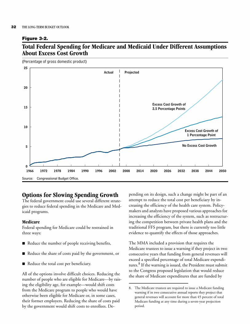
32 THE LONG-TERM BUDGET OUTLOOK
Figure 3-2.
Total Federal Spending for Medicare and Medicaid Under Different Assumptions About Excess Cost Growth(Percentage of gross domestic product)
Source: Congressional Budget Office.
1966 1972 1978 1984 1990 1996 2002 2008 2014 2020 2026 2032 2038 2044 20500
5
10
15
20
25
Excess Cost Growth of2.5 Percentage Points
No Excess Cost Growth
Excess Cost Growth of1 Percentage Point
Actual Projected
Options for Slowing Spending GrowthThe federal government could use several different strate-gies to reduce federal spending in the Medicare and Med-icaid programs.
MedicareFederal spending for Medicare could be restrained in three ways:
B Reduce the number of people receiving benefits,
B Reduce the share of costs paid by the government, or
B Reduce the total cost per beneficiary.
All of the options involve difficult choices. Reducing the number of people who are eligible for Medicare—by rais-ing the eligibility age, for example—would shift costs from the Medicare program to people who would have otherwise been eligible for Medicare or, in some cases, their former employers. Reducing the share of costs paid by the government would shift costs to enrollees. De-
pending on its design, such a change might be part of an attempt to reduce the total cost per beneficiary by in-creasing the efficiency of the health care system. Policy-makers and analysts have proposed various approaches for increasing the efficiency of the system, such as restructur-ing the competition between private health plans and the traditional FFS program, but there is currently too little evidence to quantify the effects of those approaches.
The MMA included a provision that requires the Medicare trustees to issue a warning if they project in two consecutive years that funding from general revenues will exceed a specified percentage of total Medicare expendi-tures.8 If the warning is issued, the President must submit to the Congress proposed legislation that would reduce the share of Medicare expenditures that are funded by
8. The Medicare trustees are required to issue a Medicare funding warning if in two consecutive annual reports they project that general revenues will account for more than 45 percent of total Medicare funding at any time during a seven-year projection period.

CHAPTER THREE THE LONG-TERM OUTLOOK FOR MEDICARE AND MEDICAID 33
general revenues. Various program changes could achieve that goal, including options discussed below that would increase the share of costs paid by beneficiaries.
Reduce the Number of Enrollees by Raising the Age of Eligibility. Gradually raising the eligibility age for Medi-care to 67 in 2027 would be consistent with the currently scheduled increases in the normal retirement age for So-cial Security benefits. Because the two programs largely affect the same population, some people have argued that the age requirements should be identical. Under CBO’s intermediate-spending path, raising the age of eligibility to 67 would reduce Medicare’s spending in 2050 by 0.2 percent of GDP—but Medicare spending would still climb from 2.7 percent of GDP today to 8.3 percent in 2050. Spending would fall by less than enrollment be-cause younger beneficiaries are healthier and less costly than average.
Increasing the eligibility age to 70, perhaps in conjunc-tion with a similar increase in Social Security’s normal re-tirement age, would have a larger impact on costs. After such a policy was fully phased in, Medicare spending in 2050 would be reduced by 0.9 percent of GDP. But even that relatively dramatic policy change would do little to address the long-range fiscal challenge facing Medicare, as spending for the program would still climb to 7.7 percent of GDP in 2050 under CBO’s intermediate-spending path.
The reduced spending for Medicare would be partially offset by increased spending under Medicaid and the Federal Employees Health Benefits program—both of which would be likely to cover part of the health care costs for their beneficiaries whose eligibility for Medicare had been delayed. Although spending would be reduced for the military’s TRICARE for Life program—which re-quires that enrollees be covered by Medicare—the net in-crease for all three programs would equal roughly 10 per-cent to 15 percent of the savings in Medicare.
Increasing Medicare’s eligibility age would also shift costs to enrollees and to employers. People who retired before becoming eligible for Medicare might have difficulty ob-taining health insurance, and the higher costs might lead more employers to reduce or eliminate health benefits for their retirees. Also, the affected population would have a stronger incentive to apply for Social Security disability benefits, reducing the net savings to the federal govern-ment (an effect that is not estimated here).
Reduce the Share of Costs Borne by the Government by Raising Premiums or Increasing Cost Sharing. Currently, beneficiaries pay part of the Medicare program’s costs through premiums, copayments, and deductibles. Any or all of those could be increased, reducing the percentage of total costs borne by the government. Part B premiums currently cover 25 percent of costs in that portion of the program, although that percentage will rise somewhat in the future when premiums are increased for high-income beneficiaries. Premiums under Part D will be set at a level to cover roughly a quarter of the cost of the basic pre-scription drug benefit. Increasing the premiums under Part B or Part D would reduce net government costs for Medicare by shifting a portion of the costs to beneficia-ries.
Even substantial increases in premiums are likely to have relatively modest effects on net federal costs, however. For example, if Part B premiums were increased to cover 50 percent of Part B spending, Medicare’s costs (net of pre-mium collections) would still increase from 2.4 percent of GDP today to 6.7 percent in 2050 under CBO’s inter-mediate-spending path.9
Increasing copayments or deductibles would lower the share of costs borne by the federal government and could raise the efficiency of health care or even reduce total ex-penditures by making enrollees more sensitive to the costs of health care services and thus more judicious in seeking those services. However, the effect would probably be weak in Medicare because so many beneficiaries have supplemental coverage that pays for cost sharing. Benefi-ciaries with supplemental coverage would not directly ex-perience the higher costs of care, although their supple-mental premiums would grow over time. To be most effective at bringing costs into line with the value of ser-vices, a policy of increasing beneficiaries’ cost sharing could be combined with rules that limited supplemental coverage.10
Reduce Providers’ Payment Rates. Over Medicare’s his-tory, the Congress has changed payments to health care providers to slow the growth in per capita spending—
9. That estimate assumes that enrollment in Part B would not change as a result of the higher premiums.
10. CBO has previously estimated the effects of one proposal for increasing Medicare’s cost sharing and of combining that proposal with restrictions on supplemental coverage. See Congressional Budget Office, Budget Options (February 2005), pp. 208-211.

34 THE LONG-TERM BUDGET OUTLOOK
often lowering the increase, or update, to the annual pay-ment rate that would have otherwise applied. That sort of strategy might generate savings in the short run but would do little to address the underlying sources of spending growth. Because Medicare limits the amount that providers may charge enrollees over and above the program’s payment rates, if providers could not charge enough to cover the costs of providing a service, this pol-icy could restrict Medicare beneficiaries’ access to care.
Restructure the Competition Between Private Plans and Traditional Medicare. Some policymakers and analysts have proposed converting Medicare to a “premium sup-port” system. Under premium support, the federal gov-ernment would contribute toward beneficiaries’ purchase of Medicare coverage, which they could obtain from the traditional FFS program or private plans. Federal spend-ing (net of premium collections) could be reduced if the government’s contribution toward Medicare coverage was lower than the average spending levels that would prevail under current law. Proponents contend that premium support could also reduce total spending on Medicare benefits by making beneficiaries more cost conscious in their choice of plans and stimulating greater price compe-tition among plans.
Under one general approach to premium support, the government’s contribution would be determined from the bids of competing plans. Such a system would be sim-ilar in some respects to Medicare’s current payment mechanism for private plans, but it would differ from that system in two important ways. First, the benchmarks (which determine the Medicare program’s maximum pay-ment per enrollee) would be determined from the plans’ bids rather than by a statutory formula. Second, the FFS program would be regarded as one of the bidding plans, and the projected per capita spending in that program would be regarded as its bid. Beneficiaries who enrolled in a plan whose bid was above the benchmark would pay higher premiums for their Medicare coverage, whereas those who enrolled in a plan whose bid was below the benchmark would pay lower premiums or receive addi-tional benefits. A key difference from the way the pro-gram operates under current law is that beneficiaries who chose to enroll in the FFS program would have to pay a higher premium for their Medicare coverage if they lived in an area in which the bid of that program was above the benchmark.
That approach will be tested in a six-year pilot program that was mandated by the MMA to be conducted in up to six metropolitan areas beginning in 2010. In 1999, the Bipartisan Commission on the Future of Medicare devel-oped a proposal for change based on that approach to premium support, but the proposal did not receive enough votes among the commission’s members for it to be presented as a formal recommendation to the Presi-dent and the Congress. Subsequently, some members of the commission introduced a bill, the Medicare Preserva-tion and Improvement Act of 2001 (S. 357), based on the commission’s proposal.
The effects of premium support on Medicare’s costs would depend to a great extent on how the system was designed. A key design choice is the mechanism for set-ting the government’s contribution. Several options are possible, such as determining the contribution from the average or median bid in each market area, the minimum bid in each market, or the national average bid. (In pro-posals that would use the national average bid, the gov-ernment’s contribution could be adjusted to account for geographic variations in the prices of inputs that are used to deliver Medicare services.)
In principle, a well-designed premium support system in which the government’s contribution is based on plan bids could reduce federal spending for Medicare. The magnitude of the savings is difficult to predict, however, because of uncertainty about how plans and beneficiaries would respond. To the extent that such a system in-creased the incentives for beneficiaries to be sensitive to the costs of available plans, it could also reduce total costs per beneficiary. The limited evidence from the research literature indicates that employers that have adopted comparable purchasing strategies have reduced their em-ployees’ total health care costs.11
A second general approach to premium support is to set the federal government’s contribution to an amount de-signed to meet a budgetary target. The contribution could be based initially on current spending levels but
11. For example, see Steven C. Hill and Barbara L. Wolfe, “Testing the HMO Competitive Strategy: An Analysis of Its Impact on Medical Care Resources,” Journal of Health Economics, vol. 16, no. 3 (June 1997), pp. 261-286; and David M. Cutler and Sarah J. Reber, “Paying for Health Insurance: The Trade-Off Between Competition and Adverse Selection,” Quarterly Journal of Econom-ics, vol. 113, no. 2 (May 1998), pp. 433-466.

CHAPTER THREE THE LONG-TERM OUTLOOK FOR MEDICARE AND MEDICAID 35
then updated by an amount linked to the growth in per capita GDP. Beneficiaries could use that contribution to enroll in a private plan or the FFS program and would be responsible for the portion of the plan’s premium that ex-ceeded the government’s contribution. The federal gov-ernment could be certain of controlling its spending un-der this approach, which could strengthen beneficiaries’ and health plans’ incentives to seek efficient modes of care. Depending on the level of the benefit and the re-sponse of beneficiaries, providers, and health plans, such an approach might (but would not necessarily) increase the costs borne by beneficiaries. There is little experience on which to base long-range estimates of the effects of this approach on total costs or to assess its impact on ben-eficiaries.
Other Strategies to Reduce Medicare’s Costs. Other ap-proaches that have been proposed to control costs are to modify the FFS program to incorporate strategies that are used by some innovative purchasers in the private sector. One such strategy is the use of disease managementprograms.
Disease management programs use a variety of methods to improve health outcomes for people with chronic con-ditions. Such programs vary widely, but they typically ed-ucate patients about their condition, actively monitor their symptoms, foster coordination of care among pro-viders, and encourage providers to adhere to evidence-based treatment guidelines. Proponents of disease man-agement contend that such programs can reduce health care costs by better managing patients’ conditions to pre-vent complications and by delivering care more effi-ciently. On the basis of a review of the research literature, however, CBO has concluded that there is insufficient ev-idence thus far that disease management can reduce over-all health spending.12 Additional information on the po-tential for disease management to improve health outcomes and control costs for the Medicare population will come from demonstrations of such programs that are being sponsored by the federal government.
Another possible approach to reducing Medicare’s costs is to institute changes to the FFS program that are aimed at making it more efficient. For example, Medicare could identify the most efficient providers in each community and give beneficiaries financial or other incentives to use
12. Congressional Budget Office, An Analysis of the Literature on Dis-ease Management Programs (October 13, 2004).
them, require prior authorization for selected services to reduce inappropriate use, and establish payment rates for some services through competitive bidding. Some of those approaches have been tested in a limited number of demonstrations with promising results. For example, a demonstration of competitive bidding for durable medi-cal equipment at two sites found that Medicare’s costs could be reduced without adversely affecting beneficia-ries’ quality of or access to care. Similar conclusions were reached for a demonstration in which major hospitals competed for special designation as providers of heart by-pass surgery and received global payments from Medicare that covered all hospital and physicians’ services that were used in those surgeries. There is too little evidence to esti-mate the long-term budgetary impact of more widespread implementation of such changes to the FFS program, however.
MedicaidAlthough states have wide latitude to determine the scope of the Medicaid program, there are several avenues for the federal government to reduce the growth of Medicaid spending. The federal government could reduce its con-tribution to the program through a variety of mecha-nisms. Alternatively, it could restrict mandatory benefits and coverage groups and the options available to the states for providing coverage beyond the minimum. The federal government could also shift the costs of Medicaid to beneficiaries by requiring greater cost sharing or mak-ing the requirements for receiving long-term care services more rigorous.
Reduce the Overall Federal Contribution. The federal contribution to each state is set by a formula related to the per capita income in the state. Poorer states receive higher federal matching rates, but no state can receive less than a 50 percent match. The federal government could reduce the federal match either through an across-the- board cut or by reducing the minimum rate, which ap-plied to 12 states in fiscal year 2005.
Another means of reducing the federal contribution would be to convert some or all of the funding for the program into a block grant. Such an approach would re-duce federal spending if the government set a spending limit in advance that was below the amount it would have otherwise expected to spend. States would still have to match those federal dollars, but federal funds would be cut off when the allotment was exhausted. The policy could be implemented for a category of services or popu-

36 THE LONG-TERM BUDGET OUTLOOK
lation group. For example, the federal government could cap funding for acute care services, or it could cap the federal contribution for each beneficiary, which would lessen the impact on states with growing populations.13 Converting part or all of the program into a block grant would give the federal government more control over spending and give states stronger incentives to spend funds judiciously. The approach also would end states’ in-centives to employ funding strategies that were designed to maximize federal assistance. Opponents argue that block grants could cause some states to cut needy poor individuals from the rolls.
Reduce Mandatory Benefits or Restrict Coverage. In lieu of reducing its contribution to the program, the federal government could reduce mandatory benefits and restrict coverage groups and the additional services that states could choose to offer. The federal government could also stop granting waivers of the Medicaid statute, which states have frequently used to extend coverage to new populations.
Increase Costs Shared by Beneficiaries. Under current law, states are permitted to charge beneficiaries only nom-
13. CBO has previously estimated the federal cost savings associated with one proposal for converting Medicaid payments for acute care services into a block grant. See Congressional Budget Office, Budget Options, pp. 176-177.
inal amounts (no more than $3 per service for certain population groups). The federal government could shift costs to beneficiaries by allowing or requiring states to in-stitute higher deductibles and copayments.14 To the ex-tent that beneficiaries reacted to the higher costs by using fewer services, total health care costs would also fall. Op-ponents of higher cost sharing fear that beneficiaries might forgo necessary treatment, which could lead to poorer health and possibly greater demand for more ex-tensive treatment later.
Encourage the Use of Lower-Cost Services. The federal government could also reduce spending on long-term care services by encouraging the expansion of commu-nity-based alternatives to nursing home care. Commu-nity-based care is usually much less expensive per person than institutional care is; however, the demand for com-munity-based services is greater than the demand for in-stitutional care and is more likely to substitute for infor-mal care provided in the home. That increased demand for care would offset some of the savings that would be generated by substituting community-based care for nursing home care.
14. For an estimate of the federal cost savings associated with one pro-posal for increasing copayments under Medicaid, see Congres-sional Budget Office, Budget Options, p. 175.

C HA P T E R
4The Long-Term Outlook for
Other Federal SpendingChapter 4: The Long-Term Outlook for Other Federal Spending
In 2005, about one-half of the federal government’s spending was for programs and activities other than So-cial Security, Medicare, Medicaid, and net interest on the public debt. That other half went for both discretionary programs (which are funded through the annual appro-priation process) and other mandatory programs (which are usually funded according to underlying statutes that establish eligibility and payment standards)—and in-cludes offsets for certain receipts that are recorded as neg-ative outlays. The Congressional Budget Office’s most re-cent 10-year baseline projections indicate that those programs and activities will continue to account for a siz-able share of federal spending—about 38 percent—in 2015. Consequently, the policies that guide them will continue to have a significant effect on the federal budget even as Social Security, Medicare, and Medicaid demand more resources.
Discretionary Spending One distinct pattern in the federal budget since 1962 is the diminishing share of spending provided through an-nual appropriations—spending that pays for much of what many Americans think of when they picture the ac-tivities of the federal government. Outlays for national defense, highways, the national park system, education, basic research, and the federal workforce all fall within the category of discretionary spending. As a share of the budget, such spending has declined from 68 percent in 1962 to 39 percent in 2005. Over the same period, it has also diminished in relation to the size of the economy, falling from 13 percent of gross domestic product to 8 percent (see Figure 4-1).
As a share of GDP, total discretionary spending over the past 40 years peaked at 13.6 percent in 1968, driven by defense outlays that reached 9.4 percent of GDP at the
height of the Vietnam War. Similarly, the trough in dis-cretionary spending that occurred in 1999 and 2000 re-flected the bottoming out of defense expenditures at 3.0 percent of GDP in those years. In contrast, non-defense discretionary spending as a share of GDP varied over a narrower range—from 3.2 percent (in 1999) to 5.2 percent (in 1980).
Defense Discretionary SpendingSince World War II, defense spending has fluctuated sig-nificantly. For example, it increased during the Korean War (from 1950 to 1953), the Vietnam War (from 1962 to 1973), the defense buildup during the Reagan Admin-istration (from 1982 to 1986), and toward the end of the Clinton Administration and under the Bush Administra-tion. During the intervening periods, defense spending tended to remain flat or declined. Overall, the past 60 years have been characterized by periods of slow growth or even declines (in nominal terms) in such spending.
Real (inflation-adjusted) defense spending over the past 20 years has averaged about $406 billion annually in 2005 dollars, ranging from $485 billion (in 1986 and 1987) to $322 billion (in 1998 and 1999). Over the past three years, however, defense-related outlays have ex-ceeded their 20-year average, and they are likely to re-main above it for a number of years because of the United States’ involvement in Iraq and Afghanistan.
For the purposes of its long-range budget projections, CBO developed two alternative paths for defense discre-tionary spending. The higher spending path would fol-low CBO’s projection of costs for the Bush Administra-tion’s 2006 Future Years Defense Program through 2024, including allowances for cost risks and continued addi-tional spending for military operations overseas, and thereafter maintain the 2024 real spending level (that is,

38 THE LONG-TERM BUDGET OUTLOOK
Figure 4-1.
Discretionary Spending, 1962 to 2005(Percentage of gross domestic product)
Source: Congressional Budget Office.
1962 1967 1972 1977 1982 1987 1992 1997 20020
2
4
6
8
10
12
14
Total Discretionary Outlays
Nondefense Outlays
Defense Outlays
the 2024 level increased at the rate of the consumer price index).1 Defense outlays under that approach would gradually decline from 4.0 percent of GDP in 2005 to 3.4 percent in 2015, eventually reaching 2.0 percent by 2050.
CBO’s lower path for defense spending would set a long-run target equaling the average real spending level of the past two decades ($406 billion). Because defense spend-ing is currently about 20 percent higher than that level, CBO’s lower path reduced the growth in outlays to less than the inflation rate through 2024 to reach the target level. Thereafter, spending would grow at the rate of the CPI. As a share of GDP, defense spending under that ap-proach would fall to 1.5 percent by 2050.
1. See Congressional Budget Office, The Long-Term Implications of Current Defense Plans and Alternatives: Summary Update for Fiscal Year 2006 (October 2005). Cost risks capture additional spending potentially originating from costs of weapon systems now under development that exceed early estimates, medical costs that rise more rapidly than has been projected, and the like.
Although projecting outlays as a constant share of GDP may be appropriate for some categories of spending, it seems less appropriate in the case of defense. Defense spending has trended downward fairly steadily, from 9.4 percent of GDP in 1968 to 3.8 percent in 2003 (more recent years interrupt that trend), and there is little historical basis for concluding that defense spending will continue at a fixed percentage of GDP.2
Nondefense Discretionary SpendingAppropriated spending for such government activities as those related to education, housing, highways, and na-tional parks has been a roughly constant share of GDP over the past 40 years. Except for the 1975-1983 period, during which the share of nondefense discretionary
2. If defense spending in 2050 was set to claim the same proportion of GDP that it does today, the real spending level would be more than two and a half times that of the current defense budget. In other words, maintaining defense spending at a constant share of GDP would be equivalent to funding a military force that was 25 percent to 67 percent larger than the force that was fielded in the 1980s to counter the Soviet threat.

CHAPTER FOUR THE LONG-TERM OUTLOOK FOR OTHER FEDERAL SPENDING 39
Figure 4-2.
Mandatory Spending Other Than That for Social Security, Medicare, and Medicaid, 1962 to 2005(Percentage of gross domestic product)
Source: Congressional Budget Office.
Note: The other mandatory spending shown here includes offsetting receipts.
1962 1967 1972 1977 1982 1987 1992 1997 20020
1
2
3
4
5
spending rose to about 5 percent, that category of outlays has generally ranged between 3 percent and 4 percent of GDP since 1962. For the past 20 years, the range has been from 3.2 percent to 3.9 percent, for an average of 3.6 percent. Therefore, CBO used a fixed share of GDP equal to that 20-year average as one potential path for nondefense discretionary spending.
A lower-cost alternative path developed by CBO used the baseline-related notion of constant real spending—in this case, the 2007 level of outlays adjusted for inflation.3 Un-der that approach, nondefense discretionary spending
3. The rules for constructing baselines, which are contained in the Balanced Budget and Emergency Deficit Control Act of 1985, call for inflating discretionary appropriations by using a wage inflator for personnel costs and the GDP deflator for non-pay-related expenses. For the purposes of this analysis, CBO employed the consumer price index, which is projected to rise at an annual rate of 2.2 percent by the end of the agency’s 10-year baseline projec-tion period. That rate is reasonably close to the rate of the aggre-gate inflator used under the procedures for the current baseline.
would fall from 3.9 percent of GDP in 2005 to 1.8 percent in 2050.
Other Mandatory SpendingOther mandatory spending covers an amalgam of federal mandatory programs other than Social Security, Medi-care, and Medicaid—including, for example, unemploy-ment compensation, Food Stamps, and veterans’ bene-fits—as well as receipts recorded as negative outlays, such as contributions for federal civilian and military retire-ment and payments for drilling rights on the Outer Con-tinental Shelf. Net spending for that group of activities, after peaking during the mid-1970s to the early 1980s, has moved up and down around a 20-year average of about 2.6 percent of GDP (see Figure 4-2).
CBO adopted two alternatives for its projections of the remaining mandatory spending programs and offsetting receipts. For its high and intermediate paths for such spending, CBO assumed that other mandatory outlays—including all offsetting receipts except Medicare premi-ums (discussed below)—would maintain their average of

40 THE LONG-TERM BUDGET OUTLOOK
the past two decades, or 2.6 percent of GDP. A lower spending trajectory is framed in CBO’s August 2005 baseline. There, the projections for other mandatory spending show a slightly declining claim on the economy over the next 10 years. Extrapolating a small annual de-cline over the 2006-2050 period yields a share of 1.6 percent of GDP in 2050.
Because offsetting receipts from Medicare premiums are linked to spending for the program, CBO modeled them separately, estimating them as a share of Medicare spend-ing under the various scenarios even though they are part of other mandatory spending and receipts, as categorized here. (Over the past 20 years, those premiums have con-stituted receipts of about 0.2 percent of GDP.) Under the different assumptions about Medicare spending, receipts from premiums in 2050 would range from 2.1 percent of GDP under the high-cost path to 0.7 percent under the low-cost path.
The overall projections for other mandatory spending en-compass trajectories for individual programs that are likely to be quite varied. For example, outlays for unem-ployment benefits have been relatively large when unem-ployment rates are high (as they were in 1982 and 1983, in 1992 and 1993, and in 2002 and 2003), but such
spending has moderated during periods of economic ex-pansion. In addition to the regular unemployment bene-fits that are funded through state taxes, the federal gov-ernment shares the costs of some types of benefits and often, in periods of high unemployment, extends new programs that pay 100 percent of the benefits for workers who have been unemployed for a long period. Spending for benefits as a percentage of GDP averaged 0.34 per-cent over the past 20 years but reached as high as 0.60 percent and fell as low as 0.21 percent. In contrast, spending on retirement programs for federal employees has risen at a relatively stable rate and will probably grow more slowly than the economy does because, historically, federal civilian and military employment has declined as a share of overall employment.
Spending on means-tested benefit programs such as Tem-porary Assistance for Needy Families and the Social Ser-vices Block Grant may shrink as a share of GDP either because the programs have fixed appropriations or be-cause economic growth will shrink the portion of the population that meets their eligibility thresholds for in-come and resources. However, some other mandatory spending programs, such as those providing health care for Department of Defense retirees, are likely to grow faster than the economy.

C HA P T E R
5The Long-Term Outlook for Revenues
Chapter 5: The Long-Term Outlook for Revenues
The federal government collects revenues through individual income taxes, corporate income taxes, social insurance (payroll) taxes, excise taxes, estate and gift taxes, customs duties, and miscellaneous receipts. Indi-vidual income taxes are the largest source, producing about half of all revenues and, in recent years, producing receipts totaling between 7 percent and 10 percent of gross domestic product. Social insurance taxes (mainly for Social Security and Medicare’s Hospital Insurance) are the second-largest source of receipts, making up about one-third of total revenues and equal to a little less than7 percent of GDP. Corporate income taxes contribute about 10 percent to overall revenues and are about 1 per-cent to 2 percent of GDP. Revenues from other taxes and duties and miscellaneous receipts make up the balance—about 1.5 percent of GDP.
This analysis focuses on two potential paths for federal receipts. The first path assumes that personal income tax receipts follow current law and therefore rise relative to GDP (other sources of receipts are constant as a share of GDP after 2015). Under that path, total federal revenues rise from their current level of about 17.5 percent of GDP to 23.7 percent of GDP by 2050 (see Figure 5-1). The second path assumes that the tax legislation enacted in 2001 and 2003 is extended through 2014. Under that scenario, receipts rise to 18.3 percent of GDP in 2014—the historical ratio of receipts to GDP over the past 50 years. That average level is assumed to remain constant after 2014 under the second path.
The Past 50 YearsIn the past half-century, total revenues have ranged from 16.1 percent to 20.9 percent of GDP, with no obvious trend over time (see Figure 5-2). On average, their share of GDP has hovered at about 18.5 percent. During that period, however, the various sources of revenue have changed in importance. The contribution to overall reve-
nues made by excise taxes and corporate income taxes has declined fairly steadily from a combined share of about 7 percent of GDP in 1955 to less than 3 percent today. At the same time, social insurance taxes as a percentage of GDP have grown from about 2 percent to about 6.5 per-cent. The share of individual income taxes has varied from 7.0 percent to 10.3 percent of GDP and has shown a slight upward trend.
Much of the variation in the composition of total tax rev-enues has resulted from legislative changes, as policymak-ers have altered tax rates and other parameters of the tax system. However, some of that variation has resulted from the interaction between the tax code and changes in the economy. For example, excise tax receipts tended to
Figure 5-1.
Total Federal Revenues UnderAlternative Paths(Percentage of gross domestic product)
Source: Congressional Budget Office.
Note: The historical-average values are based on 30-year historical averages.
2005 2010 2015 2020 2025 2030 2035 2040 2045 20500
5
10
15
20
25
30
Under Current Law
Based on Historical Average

42 THE LONG-TERM BUDGET OUTLOOK
Figure 5-2.
Sources of Federal Revenues Over the Past 50 Years(Percentage of gross domestic product)
Source: Congressional Budget Office.
1955 1960 1965 1970 1975 1980 1985 1990 1995 2000 20050
2
4
6
8
10
12
14
16
18
20
22
Total
Individual Income Taxes
Social Insurance(Payroll) Taxes
Corporate Income Taxes
decline over time as a percentage of GDP because many are specific levies (such as cents per gallon of gasoline) and thus diminished in importance as the economy expe-rienced inflation. In contrast, income tax receipts tended to increase relative to GDP when inflation caused various thresholds in the income tax system to decline in real (in-flation-adjusted) terms and therefore boosted the amount of income subject to taxation at higher rates. Over the years, legislators have often changed those parameters of the tax system to offset the impact of such economic changes on taxes. In the case of the individual income tax, much of the system was eventually indexed to prevent inflation from raising that levy’s share of GDP. Yet with-out adjustments, a host of characteristics of the current tax system continue to interact with economic conditions and cause receipts on net to grow faster than GDP.
Potential Future Paths for Federal Revenues As in the past, all sources of revenue will continue to be subject to legislative discretion over the long term. How-ever, in the absence of legislative action, the individual in-come tax system has the most potential to increase the ra-
tio of revenues to GDP because of the various ways in which its structure interacts with the economy.
First, that system is progressive, which means that house-holds with higher incomes are taxed at higher rates. Con-sequently, as GDP and individual incomes grow, a larger and larger proportion will be subject to higher tax rates. The growth of income will both increase the amount of income taxed at the highest rates and decrease the amount of earned income tax credits claimed on low-income tax returns. Because much of the tax system is indexed for inflation, that phenomenon will occur prima-rily with respect to real GDP growth. But some effect from inflation on the parts of the regular income tax sys-tem that are not indexed will cause additional, although modest, increases in receipts relative to GDP by 2050.
Second, the individual income tax system includes an al-ternative minimum tax, which subjects more taxpayers and a greater fraction of income to higher rates as GDP grows. The AMT is a parallel income tax system with fewer exemptions, deductions, and rates than the regular income tax. Households must calculate their tax liability (the amount they owe) under both the AMT and the reg-

CHAPTER FIVE THE LONG-TERM OUTLOOK FOR REVENUES 43
ular income tax and pay the higher of the two.1 The AMT is not indexed for inflation; therefore, sustained inflation causes it to affect more taxpayers (as nominal income rises over time) and to claim an ever-larger share of GDP.
Third, current tax law provides for rates to increase in 2011. Most of the provisions in the Economic Growth and Tax Relief Reconciliation Act of 2001 (EGTRRA) and the Jobs and Growth Tax Relief Reconciliation Act of 2003 (JGTRRA) are scheduled to expire at the end of 2010; other provisions expire even sooner. As the tax code reverts to prior law, tax rates will rise, some credits will shrink, and thresholds for certain rates will shift. Those changes will increase the level of receipts as a share of GDP, both immediately and in the future.
Fourth, between now and 2050, the Treasury will receive some tax revenues that have essentially been deferred. Contributions to retirement plans, such as 401(k) and individual retirement accounts, and contributions to employer-sponsored defined-benefit plans are tax-exempt when they are made. The income earned on assets in those accounts also is exempt, but withdrawals from those plans are taxable. Those sums will become a rising portion of taxable income as the baby boomers retire, which will tend to boost receipts relative to GDP.
At least one factor will reduce receipts, however, causing individual income tax revenues (as well as revenues from Social Security and Medicare payroll taxes) to shrink as a percentage of GDP during the next half-century. The share of employees’ compensation that is paid in the form of wages and salaries (which are subject to income and payroll taxes) is projected by the Congressional Budget Office to decrease over time, in part because of the rising costs of nontaxable fringe benefits, such as employer-paid health insurance. That declining share will reduce taxable income and therefore tax revenues relative to GDP.
Illustrative Revenue PathsThe long-term budget scenarios outlined in Chapter 1 assume one of two possible paths for revenues, based on
1. Technically, a taxpayer owes the regular income tax plus any amount by which the AMT exceeds the regular tax. For more information on the AMT, see Congressional Budget Office, The Alternative Minimum Tax, Revenue and Tax Policy Brief No. 4 (April 15, 2004).
different approaches to tax policy. One option is to assume enactment of a series of legislative changes that would keep receipts close to their historical average share of GDP. That outcome could be achieved either through changes in the individual income tax system or through reductions in other taxes to offset the expected rise in individual income taxes under current law. Consequently, the first path is one in which receipts remain steady at 18.3 percent of GDP—the average of the past 30 years—beginning in 2014 (see Figure 5-2). That percentage is close to the level that would be achieved in 2014 if the provisions of EGTRRA and JGTRRA were extended.
The second path is an extrapolation of current law. It assumes that the provisions of EGTRRA and JGTRRA expire (or “sunset”) as scheduled, that policymakers do not modify the AMT, and that no changes are made in tax law to slow the automatic increase in taxes that results from the interaction of economic growth and the pro-gressive structure of the income tax. Although there is some tendency over the long term for taxable wage and salary income to decline as a proportion of compensa-tion, the overwhelming effect of the tax system’s current-law features is to raise receipts relative to GDP. Conse-quently, receipts rise to 23.7 percent of GDP by 2050 in the current-law path and are 5.4 percentage points higher than in the historical-average path.
Details of the Current-Law PathIn the current-law path, the individual income tax is responsible for the rise in revenue relative to GDP. Two of the factors that drive the increase in individual income tax receipts as a share of GDP are currently the subject of considerable legislative interest: the scheduled expiration of EGTRRA and JGTRRA and the mounting effects of the AMT.
Comparing the current-law path with one in which EGTRRA and JGTRRA are permanently extended high-lights the sunset aspects of the two laws (see Figure 5-3). The expiration of EGTRRA and JGTRRA contributes a bit more than 1 percentage point of the higher receipts-to-GDP ratio in 2015, declining to a bit less than 1 per-centage point in 2050. The explanation for that ebbing effect lies in the AMT. As more and more taxpayers become subject to the AMT, the tax increases triggered by the sunset of EGTRRA and JGTRRA affect fewer and fewer taxpayers.

44 THE LONG-TERM BUDGET OUTLOOK
Figure 5-3.
Individual Income Tax Liabilities Under Current Law and Under aPermanent Extension of EGTRRAand JGTRRA(Percentage of gross domestic product)
Source: Congressional Budget Office.
Note: EGTRRA = Economic Growth and Tax Relief Reconciliation Act of 2001; JGTRRA = Jobs and Growth Tax Relief Recon-ciliation Act of 2003.
The AMT can be modified in various ways, each of which yields a different measure of its effect. For the pur-poses of illustration, CBO measured the impact of that tax relative to a policy change in which the higher AMT exemption in effect for 2005 is made permanent and all AMT parameters are indexed for inflation beginning in 2006 (see Figure 5-4).2 If the lower marginal tax rates in EGTRRA and JGTRRA were not extended, inflation would have only a small effect on the AMT in 2015. Over time, however, inflation has a three-pronged effect: it makes more taxpayers subject to the AMT, it causes a smaller proportion of their income to be exempt from the tax, and it pushes more taxpayers into the higher AMT tax brackets. Consequently, by 2050, the effect of infla-tion on the AMT under current law will make receipts as a share of GDP about 2 percentage points higher than they would be if the AMT was indexed.
Taken together, the expiration of EGTRRA and JGTRRA and the effect of inflation on the AMT will
2. That illustration also incorporates the assumption that the AMT does not limit personal credits.
2005 2010 2015 2020 2025 2030 2035 2040 2045 20500
2
4
6
8
10
12
14
16
Under Current Law
With Permanent Extensionof EGTRRA and JGTRRA
raise receipts as a share of GDP by about 2 percentage points in 2015, CBO estimates (see Figure 5-5). In 2050, their combined effect will enlarge that share by almost 4 percentage points. The simultaneous effects of inflation on the AMT and the expiration of EGTRRA and JGTRRA exceed the sum of the effects of each factor individually because the two sets of effects interact. With lower tax rates in place, as provided for in EGTRRA and JGTRRA, the AMT will affect more taxpayers than it would if the old tax system was in place. Similarly, with-out an AMT, the tax reductions in EGTRRA and JGTRRA would have a greater impact.
If those two tax laws are made permanent and the AMT is modified, the remaining increase in receipts as a share of GDP will be largely attributable to the progressive rate structure of the tax system. The growth of GDP and its effects on the rates at which income is taxed will increase that share by 2 percentage points by 2050 compared with the share that would result if individual income tax receipts remained steady relative to GDP. Most of that 2 percentage-point increase is commonly referred to as “real bracket creep” as an analogy to the bracket creep that used to occur as a result of inflation before the tax system was indexed. But because even a low annual rate of infla-
Figure 5-4.
Individual Income Tax Liabilities Under Current Law and Under aModified AMT(Percentage of gross domestic product)
Source: Congressional Budget Office.
Note: AMT = alternative minimum tax.
2005 2010 2015 2020 2025 2030 2035 2040 2045 20500
2
4
6
8
10
12
14
16
Under Current Law
With AMT Modification

CHAPTER FIVE THE LONG-TERM OUTLOOK FOR REVENUES 45
Figure 5-5.
Individual Income Tax Liabilities Under Three Policy Alternatives(Percentage of gross domestic product)
Source: Congressional Budget Office.
Note: EGTRRA = Economic Growth and Tax Relief Reconciliation Act of 2001; JGTRRA = Jobs and Growth Tax Relief Recon-ciliation Act of 2003; AMT = alternative minimum tax.
tion amounts to a significant increase in prices by 2050, some of the effect shown in Figure 5-5 is attributable to inflation’s effects on the remaining unindexed provisions of the tax code. If, in addition to extending EGTRRA and JGTRRA and indexing the AMT, policymakers indexed the tax code to the growth of real income, much of the remaining difference between the current-law and historical-average paths would disappear.
Implications of the Current-Law PathContinuation of current law would raise receipts relative to GDP. In the process, it would have important implica-tions for taxpayers: more households would have to pay income taxes, more of those households would be subject to higher tax rates, and a smaller proportion of each household’s income would fall in the lower and zero tax brackets than is currently the case.
The effect of the AMT on taxpayers would be especially significant. By 2050, roughly 15 percent of individual income tax liability would be generated by the AMT, compared with about 2 percent today (see Figure 5-6). However, roughly 65 percent of the nation’s households would be subject to the AMT in that year, a dramatic increase from the current 2 percent. Clearly, the AMT’s contribution to receipts, although large, gives little indi-cation of the number of people affected by the tax. The
2005 2010 2015 2020 2025 2030 2035 2040 2045 20500
2
4
6
8
10
12
14
16
Under Current Law
With PermanentExtension of EGTRRA
and JGTRRA
With PermanentExtension of EGTRRA
and JGTRRA andAMT Modification
reason is that taxpayers would still have to pay the regular income tax, but an increasingly large number would also have to pay an additional AMT.
Real bracket creep in the current-law path would move more income into higher tax brackets. The share of total taxable income taxed at the regular rates of 15 percent and 28 percent is projected to fall from just under 75 per-cent in 2015 to just under 66 percent by 2050. As a result of that shift, by 2050, an additional 9 percent of income would be taxed at the higher rates of 31 percent, 33 per-cent, 36 percent, and 39.6 percent.
Real income growth would also substantially reduce the role of many tax preferences. For example, between now and 2050, the share of households with income low enough to claim the earned income tax credit would fall from about 14 percent of tax returns to 4 percent. The share of returns claiming the child tax credit also would plummet, from 20 percent to less than 2 percent. In addi-tion, inflation and real wage growth would affect the threshold at which Social Security benefits became sub-ject to taxation, because that threshold is not indexed. As a result, the proportion of total Social Security benefits that are taxed will rise from about 24 percent today to about 50 percent by 2050.
Figure 5-6.
The AMT’s Impact on Individual Income Tax Liabilities UnderCurrent Law(Percent)
Source: Congressional Budget Office.
Note: AMT = alternative minimum tax.
2005 2010 2015 2020 2025 2030 2035 2040 2045 20500
10
20
30
40
50
60
70
Share of HouseholdsAffected by the AMT
AMT Liabilityas a Share ofTotal Liability

46 THE LONG-TERM BUDGET OUTLOOK
Other TaxesAs noted above, CBO projects that payroll tax receipts will decline slightly over the next half-century because of the reduction in the share of compensation paid as tax-able wages and salaries. That decline, though noticeable, is small (see Figure 5-7).
Other taxes also will tend to change under current law, but CBO does not explicitly address them in this analysis. Unless altered by legislation, excise taxes will tend to decline in importance. Under the assumption that EGTRRA expires, estate and gift taxes will tend to rise as the real value of estates increases with higher levels of in-come and wealth. The course of corporate taxes through 2050 is uncertain, even assuming no changes in tax law. Because the corporate tax rate structure is basically flat, bracket creep will have little effect. But at the same time, some long-term erosion has occurred in the amount of corporate income that is subject to taxation.
For the purposes of this analysis, CBO assumes that reve-nue sources other than the individual income tax and payroll taxes remain constant as a percentage of GDP. Because those other sources will collectively respond to the growth of income in either offsetting or unknown ways, that assumption is probably a reasonable approxi-mation of the most likely outcomes over the long run.
Figure 5-7.
Individual Income Taxes and Payroll Taxes Under the Current-Law andHistorical-Average Scenarios(Percentage of gross domestic product)
Source: Congressional Budget Office.
Note: The historical-average values are based on 30-year historical averages, beginning in 2014.
2005 2010 2015 2020 2025 2030 2035 2040 2045 20500
2
4
6
8
10
12
14
16Individual Income
Taxes Under Current Law
Individual Income TaxesBased on Historical Average
Payroll Taxes(Under either scenario)
Appendix: Details of theLong-Term Budget Scenarios
This appendix provides more detail about the illus-trative long-term budget scenarios used in this analysis. The assumptions about various types of spending and tax revenues that underlie those scenarios are outlined in
Table A-1. The paths for spending, revenues, gross domestic product, and the total budget surplus or deficit under those scenarios are shown in Figures A-1 through A-9.

48 THE LONG-TERM BUDGET OUTLOOK
Table A-1.
Assumptions Underlying CBO’s Long-Term Budget Scenarios
Continued
Scenario 1: Higher Spending/Lower Revenues
Scenario 2:Intermediate Spending/Lower Revenues
Scenario 3:Lower Spending/Lower Revenues
Scenario 4: Higher Spending/Higher Revenues
Scenario 5:Intermediate Spending/Higher Revenues
Scenario 6:Lower Spending/Higher Revenues
Outlays
Social Security Benefits paid as scheduled under current law
Benefits paid as scheduled under current law
Benefits paid as scheduled under current law
Benefits paid as scheduled under current law
Benefits paid as scheduled under current law
Benefits paid as scheduled under current law
Medicare Excess cost growth of 2.5 percentage points
Excess cost growth of 1.0 percentage point
No excess cost growth
Excess cost growth of 2.5 percentage points
Excess cost growth of 1.0 percentage point
No excess cost growth
Medicaid Excess cost growth of 2.5 percentage points
Excess cost growth of 1.0 percentage point
No excess cost growth
Excess cost growth of 2.5 percentage points
Excess cost growth of 1.0 percentage point
No excess cost growth
Other Mandatory Programsa
Stabilize at the 2005 level as a percentage of GDP
Stabilize at the 2005 level as a percentage of GDP
Decline by 1 percent annually as a percentage of GDP
Stabilize at the 2005 level as a percentage of GDP
Stabilize at the 2005 level as a percentage of GDP
Decline by 1 percent annually as a percentage of GDP
Defense Programs
Follow FYDP through 2024, then grow at rate of CPI
Phase down gradually to $406 billion (in 2005 dollars) in 2024 and then grow at rate of CPI
Phase down gradually to $406 billion (in 2005 dollars) in 2024 and then grow at rate of CPI
Follow FYDP through 2024, then grow at rate of CPI
Phase down gradually to $406 billion (in 2005 dollars) in 2024 and then grow at rate of CPI
Phase down gradually to $406 billion (in 2005 dollars) in 2024 and then grow at rate of CPI
Nondefense DiscretionaryPrograms
Phase down to historical share of GDP (3.6 percent) by 2007 and remain there
Phase down to historical share of GDP (3.6 percent)by 2007 and remain there
Grow at rate of CPI after 2007
Phase down to historical share of GDP (3.6 percent)by 2007 and remain there
Phase down to historical share of GDP (3.6 percent) by 2007 and remain there
Grow at rate of CPI after 2007

APPENDIX DETAILS OF THE LONG-TERM BUDGET SCENARIOS 49
Table A-1.
Continued
Source: Congressional Budget Office.
Note: GDP = gross domestic product; FYDP = Future Years Defense Program; CPI = consumer price index.
a. Excludes premiums paid by Medicare beneficiaries, which are recorded in the budget as offsetting receipts.
Scenario 1: Higher Spending/Lower Revenues
Scenario 2:Intermediate Spending/Lower Revenues
Scenario 3:Lower Spending/Lower Revenues
Scenario 4: Higher Spending/Higher Revenues
Scenario 5:Intermediate Spending/Higher Revenues
Scenario 6:Lower Spending/Higher Revenues
Revenues
Individual Income Taxes
Gradually rise as a percentage of GDP until 2014, then adjusted so total federal revenues equal 18.3 percent of GDP
Gradually rise as a percentage of GDP until 2014, then adjusted so total federal revenues equal 18.3 percent of GDP
Gradually rise as a percentage of GDP until 2014, then adjusted so total federal revenues equal 18.3 percent of GDP
Follow current law Follow current law Follow current law
Social Insurance (Payroll) Taxes
Follow current law Follow current law Follow current law Follow current law Follow current law Follow current law
Other Taxes Remain fixed at2014 level as a percentage of GDP
Remain fixed at2014 level as a percentage of GDP
Remain fixed at2014 level as a percentage of GDP
Remain fixed at 2014 level as a percentage of GDP
Remain fixed at 2014 level as a percentage of GDP
Remain fixed at 2014 level as a percentage of GDP

50 THE LONG-TERM BUDGET OUTLOOK
Figure A-1.
Social Security Spending Under CBO’s Long-Term Budget Scenarios (Percentage of gross domestic product)
Source: Congressional Budget Office.
Note: For information about the scenarios, see Table A-1 and Chapter 1.
1962 1970 1978 1986 1994 2002 2010 2018 2026 2034 2042 20500
2
4
6
8
10
12
14
All Scenarios
Actual Projected

APPENDIX DETAILS OF THE LONG-TERM BUDGET SCENARIOS 51
Figure A-2.
Medicare Spending Under CBO’s Long-Term Budget Scenarios (Percentage of gross domestic product)
Source: Congressional Budget Office.
Notes: Scenario 1 = higher spending/lower revenues
Scenario 2 = intermediate spending/lower revenues
Scenario 3 = lower spending/lower revenues
Scenario 4 = higher spending/higher revenues
Scenario 5 = intermediate spending/higher revenues
Scenario 6 = lower spending/higher revenues
For information about the scenarios, see Table A-1 and Chapter 1.
1962 1970 1978 1986 1994 2002 2010 2018 2026 2034 2042 20500
2
4
6
8
10
12
14
Scenarios1 and 4
Actual Projected
Scenarios2 and 5
Scenarios3 and 6

52 THE LONG-TERM BUDGET OUTLOOK
Figure A-3.
Federal Medicaid Spending Under CBO’s Long-Term Budget Scenarios (Percentage of gross domestic product)
Source: Congressional Budget Office.
Notes: Scenario 1 = higher spending/lower revenues
Scenario 2 = intermediate spending/lower revenues
Scenario 3 = lower spending/lower revenues
Scenario 4 = higher spending/higher revenues
Scenario 5 = intermediate spending/higher revenues
Scenario 6 = lower spending/higher revenues
For information about the scenarios, see Table A-1 and Chapter 1.
1962 1970 1978 1986 1994 2002 2010 2018 2026 2034 2042 20500
2
4
6
8
10
12
14
Scenarios1 and 4
Actual Projected
Scenarios2 and 5
Scenarios 3 and 6

APPENDIX DETAILS OF THE LONG-TERM BUDGET SCENARIOS 53
Figure A-4.
Defense Spending Under CBO’s Long-Term Budget Scenarios (Percentage of gross domestic product)
Source: Congressional Budget Office.
Notes: Scenario 1 = higher spending/lower revenues
Scenario 2 = intermediate spending/lower revenues
Scenario 3 = lower spending/lower revenues
Scenario 4 = higher spending/higher revenues
Scenario 5 = intermediate spending/higher revenues
Scenario 6 = lower spending/higher revenues
For information about the scenarios, see Table A-1 and Chapter 1.
1962 1970 1978 1986 1994 2002 2010 2018 2026 2034 2042 20500
2
4
6
8
10
12
14
Scenarios 1 and 4
Actual Projected
Scenarios 2, 3, 5, and 6

54 THE LONG-TERM BUDGET OUTLOOK
Figure A-5.
Other Federal Spending Under CBO’s Long-Term Budget Scenarios (Percentage of gross domestic product)
Source: Congressional Budget Office.
Notes: Other federal spending comprises nondefense discretionary spending; mandatory spending for programs other than Social Security, Medicare, and Medicaid; and offsetting receipts. It excludes net interest.
Scenario 1 = higher spending/lower revenues
Scenario 2 = intermediate spending/lower revenues
Scenario 3 = lower spending/lower revenues
Scenario 4 = higher spending/higher revenues
Scenario 5 = intermediate spending/higher revenues
Scenario 6 = lower spending/higher revenues
For information about the scenarios, see Table A-1 and Chapter 1.
1962 1970 1978 1986 1994 2002 2010 2018 2026 2034 2042 20500
2
4
6
8
10
12
14
Scenarios1 and 4
Actual Projected
Scenarios 2 and 5
Scenarios 3 and 6

APPENDIX DETAILS OF THE LONG-TERM BUDGET SCENARIOS 55
Figure A-6.
Federal Interest Spending Under CBO’s Long-Term Budget Scenarios (Percentage of gross domestic product)
Source: Congressional Budget Office.
Notes: Scenario 1 = higher spending/lower revenues
Scenario 2 = intermediate spending/lower revenues
Scenario 3 = lower spending/lower revenues
Scenario 4 = higher spending/higher revenues
Scenario 5 = intermediate spending/higher revenues
Scenario 6 = lower spending/higher revenues
For information about the scenarios, see Table A-1 and Chapter 1.
1962 1970 1978 1986 1994 2002 2010 2018 2026 2034 2042 2050-10
-5
0
5
10
15
Scenario 1Scenario 5
Scenario 4
Scenario 3
Scenario 6
Scenario 2
Actual Projected

56 THE LONG-TERM BUDGET OUTLOOK
Figure A-7.
Individual Income Tax Revenues Under CBO’s Long-Term Budget Scenarios (Percentage of gross domestic product)
Source: Congressional Budget Office.
Notes: Scenario 1 = higher spending/lower revenues
Scenario 2 = intermediate spending/lower revenues
Scenario 3 = lower spending/lower revenues
Scenario 4 = higher spending/higher revenues
Scenario 5 = intermediate spending/higher revenues
Scenario 6 = lower spending/higher revenues
For information about the scenarios, see Table A-1 and Chapter 1.
1962 1970 1978 1986 1994 2002 2010 2018 2026 2034 2042 20500
5
10
15
20
25
30
Scenarios 4, 5, and 6
Actual Projected
Scenarios 1, 2, and 3

APPENDIX DETAILS OF THE LONG-TERM BUDGET SCENARIOS 57
Figure A-8.
Real Gross Domestic Product Under CBO’s Long-Term Budget Scenarios (Billions of 2005 dollars)
Source: Congressional Budget Office.
Note: For information about the scenarios, see Table A-1 and Chapter 1.
1962 1970 1978 1986 1994 2002 2010 2018 2026 2034 2042 20500
5
10
15
20
25
30
35Actual Projected

58 THE LONG-TERM BUDGET OUTLOOK
Figure A-9.
Total Surplus or Deficit Under CBO’s Long-Term Budget Scenarios (Percentage of gross domestic product)
Source: Congressional Budget Office.
Notes: Scenario 1 = higher spending/lower revenues
Scenario 2 = intermediate spending/lower revenues
Scenario 3 = lower spending/lower revenues
Scenario 4 = higher spending/higher revenues
Scenario 5 = intermediate spending/higher revenues
Scenario 6 = lower spending/higher revenues
For information about the scenarios, see Table A-1 and Chapter 1.
1962 1970 1978 1986 1994 2002 2010 2018 2026 2034 2042 2050-35
-30
-25
-20
-15
-10
-5
0
5
10
15
Scenario 1
Scenario 5
Scenario 4
Scenario 3
Scenario 6
Scenario 2
Actual Projected