The Macro Impact of Short-Termism

Stephen J. Terry⇤

Boston University

June 2017

Abstract

R&D investment reduces current profits, so short-term pressure on man-agers to hit profit targets may distort R&D. In the data, firms just meetingWall Street forecasts have lower R&D growth, while managers just missingreceive lower pay. However, short-termist distortions might wash out in the ag-gregate, so to quantify their macro impact I build and estimate a growth modelin which managers of heterogeneous firms choose R&D while facing firm-levelshocks and profit targets derived from rational forecasts. Short-termism in-creases R&D volatility, lowering growth by 0.1% annually and output by 6%over 100 years, a sizable cost to the macroeconomy.

Keywords: Short-Termism, Heterogeneous Firms, Endogenous Growth, AgencyConflicts, Earnings ManipulationJEL Codes: E20, G30, O40

⇤A previous version circulated as “The Macro Impact of Firm Earnings Targets.” Pleasefind the latest draft, as well as online appendixes, at http://people.bu.edu/stephent. Email:stephent@bu.edu. Mailing Address: Boston University, Dept. of Economics, 270 Bay State Rd.,Room 406, Boston, MA 02215. I gratefully acknowledge funding as a Bradley Fellow from theStanford Institute for Economic Policy Research. I benefited from advice from many including NickBloom, Pete Klenow, Bob Hall, Monika Piazzesi, Nir Jaimovich, Ed Knotek, Itay Saporta-Eksten,Brent Bundick, Julia Thomas, Aubhik Khan, Jon Willis, Jordan Rappaport, Chris Tonetti, MikeDinerstein, John Mondragon, Nicola Bianchi, Ivan Marinovic, Adam Guren, Simon Gilchrist, GadiBarlevy, and many seminar and conference participants.

1

Managers of the largest firms in the US economy face relentless scrutiny of their

short-term profits. The managing director of McKinsey & Company recently sum-

marized the situation, writing “the mania over quarterly earnings [profits] consumes

extraordinary amounts of senior executive time and attention.” Commentators have

long suspected that short-termist profit pressures might lead managers to sacrifice

investment, innovation, or even financial stability.1 However, short-termist pressures

might not matter at all for the macroeconomy if they wash out due to aggregation

or equilibrium forces. In this paper, I argue using a quantitative macro model that

short-termism does in fact matter, costing the entire economy lost growth each year.

Each fiscal period, public firms must disclose their profits or earnings. Small

armies of analysts at stock brokerages forecast profits, and the financial press widely

reports a consensus forecast for a given firm. During earnings season when profits are

revealed, firm performance is routinely compared to these short-term targets. Around

90% of recently surveyed US managers report pressure to meet short-term profit

targets (Graham et al., 2005), and the pattern of firm profits in the data supports

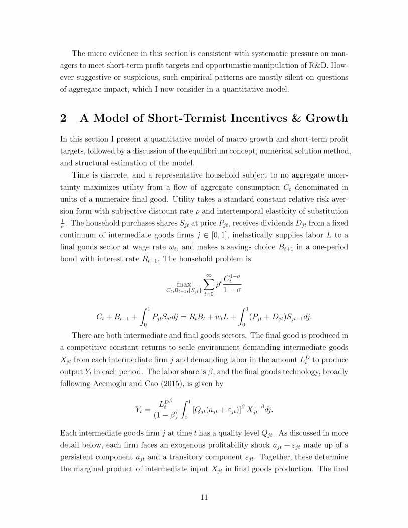
this notion. Figure 1 plots the distribution of forecast errors, realized profits minus

consensus analyst forecasts, for a large panel of US public firms over the past 30

years.2 Two facts stand out. First, firm profits bunch just above forecasts or at zero

in the error distribution.3 Second, relatively few firm-years display narrow misses.

Figure 1 suggests some form of systematic pressure to meet profit targets.

In the face of short-term profit pressure, long-term investments like research and

development (R&D) provide a choice target for manipulation, since they equal around

33% of profits for a typical firm.4 While the benefits of R&D may appear much

later or fail to materialize altogether, the costs must be borne today through lower

profits.5 Some firms must therefore choose between cuts to R&D or meeting their

profit target. Almost half of surveyed US executives report that they would prefer to

1See Stein (1989), Haldane and Davies (2011), Schwenkler et al. (2015), Budish et al. (2015),Rahmandad et al. (2014), Gigler et al. (2014), Kanodia and Sapra (2015), Marko↵ (1990), Mayer(2012), or Michie (2001). The quote is from Barton (2011).

2More details on data sources and variable definitions are in Section 1 and Appendix A.3The McCrary (2008) sorting test strongly rejects continuity at zero. Marinovic et al. (2012)

and Hong and Kacperczyk (2010) overview analyst earnings forecasts. Burgstahler and Chuk (2013)emphasizes that the discontinuity in Figure 1 is robust. See Garicano et al. (2013), Gourio andRoys (2014), Chetty et al. (2011), Daly et al. (2012), and Allen and Dechow (2013) for evidenceof similar bunching in French firm sizes around regulatory thresholds, Danish income around taxkinks, nominal wage changes around zero, and even marathon finish times around focal points.

4This statistic is the median ratio of R&D expenditures to profits, drawn from my combinedCompustat-I/B/E/S database detailed in Section 1 and Appendix A.

5Since SFAS Rule No. 2 in 1974, the US Generally Accepted Accounting Principles (US GAAP)have dictated that R&D generally be expensed or subtracted from earnings.

2

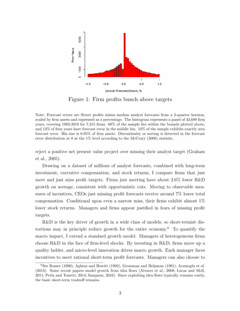
Figure 1: Firm profits bunch above targets

Note: Forecast errors are Street profits minus median analyst forecasts from a 2-quarter horizon,scaled by firm assets and expressed as a percentage. The histogram represents a panel of 43,688 firmyears, covering 1982-2010 for 7,215 firms. 68% of the sample lies within the bounds plotted above,and 13% of firm years have forecast error in the middle bin. 10% of the sample exhibits exactly zeroforecast error. Bin size is 0.05% of firm assets. Discontinuity or sorting is detected in the forecasterror distribution at 0 at the 1% level according to the McCrary (2008) statistic.

reject a positive net present value project over missing their analyst target (Graham

et al., 2005).

Drawing on a dataset of millions of analyst forecasts, combined with long-term

investment, executive compensation, and stock returns, I compare firms that just

meet and just miss profit targets. Firms just meeting have about 2.6% lower R&D

growth on average, consistent with opportunistic cuts. Moving to observable mea-

sures of incentives, CEOs just missing profit forecasts receive around 7% lower total

compensation. Conditional upon even a narrow miss, their firms exhibit almost 1%

lower stock returns. Managers and firms appear justified in fears of missing profit

targets.

R&D is the key driver of growth in a wide class of models, so short-termist dis-

tortions may in principle reduce growth for the entire economy.6 To quantify the

macro impact, I extend a standard growth model. Managers of heterogeneous firms

choose R&D in the face of firm-level shocks. By investing in R&D, firms move up a

quality ladder, and micro-level innovation drives macro growth. Each manager faces

incentives to meet rational short-term profit forecasts. Managers can also choose to

6See Romer (1990), Aghion and Howitt (1992), Grossman and Helpman (1991), Acemoglu et al.(2013). Some recent papers model growth from idea flows (Alvarez et al., 2008; Lucas and Moll,2011; Perla and Tonetti, 2014; Sampson, 2016). Since exploiting idea flows typically remains costly,the basic short-term tradeo↵ remains.

3

distort their reported profits using a flexible paper manipulation tool.

With this framework, I structurally estimate the micro shock process as well as the

size of short-termist pressure on managers using GMM. I target the micro covariance

matrix of forecast errors, R&D growth, and sales growth together with the long-term

US growth rate. In the estimated model, managers perceive costs of missing a profit

target equal to around 3.6% of yearly sales, a substantial consideration. Although the

model was not estimated to do so, my structure with short-term targets reproduces a

range of basic data facts including forecast error bunching, the discontinuity in R&D

growth, the dynamics of R&D, and cross-industry heterogeneity in bunching.

Short-term pressure is present each period and embodied in rational profit fore-

casts. Any permanent cut to R&D would be incorporated into the forecasts over time

and o↵er little improvement in the ability to meet targets in the longer term. Natu-

rally, therefore, the mean level of R&D changes very little in response to this constant

pressure. By contrast, targets do increase the volatility or standard deviation of R&D

by around 25% as managers often cut and then later splurge on R&D in response

to short-term shocks. Decades of empirical research on R&D, patenting, and firm

growth suggest that firms face diminishing returns to R&D, implying in my model

that higher R&D volatility reduces overall innovation.7 More plainly, the model sim-

ply assumes that R&D projects are more e�cient with stable funding streams than

if they are continually subjected to sharp cuts and quick rebounds in funding.

Overall, the presence of short-termist pressure causes growth to drop by almost

0.1% per year, leading to around 6% lower output over a century. In the baseline

model, households su↵er a loss in welfare of around 0.5% or $50 billion of lost con-

sumption each year. For each household in the US, short-term targets therefore cause

a sizable loss of over $400 of consumption annually.8 For some comparison, recent

quantitative estimates place the welfare costs of business cycles at around 0.1-1.8%,

the static gains from trade in the area of 2.0-2.5%, and the welfare costs of inflation

near 1%.9 These figures are roughly the same order of magnitude as my estimates of

the costs of short-termism.

My baseline results delineate the costs of short-term targets. However, managers

may be badly behaved, in which case short-term pressures may provide discipline even

7See Blundell et al. (2002), Klette and Kortum (2004), or Acemoglu et al. (2013).8US consumption was around $11.5 trillion in 2013 according to the BEA as of March 2014, so the

0.44% loss in the model equals a loss of around $51 billion each year. Based on US Census Bureauestimates, the number of households in the US in 2013 was approximately 122 million (see the 2016version of Table HH-1 based on the ASEC supplement to the CPS), leading to a total consumptionloss of slightly over $400 per household annually in 2013 dollars due to short-term targets.

9For more details and exact references, see the explicit comparisons made in Section 4.

4

while distorting R&D and growth. I extend the model to incorporate two forms of

manager misbehavior: shirking and empire building. With badly behaved managers,

short-term targets may increase firm value. However, the exact assumptions matter

for the net social welfare impact. If managers are characterized by shirking problems,

then targets typically push up consumption levels and overall welfare. By contrast, if

managers exhibit empire building tendencies, then targets tend to push down R&D

further away from socially optimal levels and reduce consumer welfare. While the

net social welfare impact, the appropriate guide for policymaking, is ambiguous in

general, the core prediction of the model remains: short-term targets distort R&D

and reduce growth.

Overall my analysis suggests that the benefits of liquid capital markets, trans-

parent reporting, and disciplined managers do not come for free. Instead, closely

associated short-termist behavior creates a sizable drag on growth.

Section 1 analyzes short-term targets in the data. Section 2 presents my macro

growth model. Section 3 checks the model against some basic facts from the micro

data. Section 4 reports the costs of short-termism. Section 5 subjects the quantita-

tive estimates to a series of robustness checks. Section 6 explores potential benefits

from targets with manager misbehavior. Section 7 concludes. Online appendixes de-

scribe the data (Appendix A), theory (Appendix B), and numerical solution method

(Appendix C).

1 Short-Term Targets in the Data

I draw on two main data sources. First, I exploit millions of profit forecasts at

the firm-analyst level from the Institutional Brokers Estimates System (I/B/E/S)

database. Realized values of firm “Street” profits accompany analyst forecasts in

I/B/E/S.10 I also use Compustat data from annual US public firm income statements.

Linking the I/B/E/S and Compustat datasets results in a panel of around 25,000 firm-

fiscal year observations with consensus analyst forecasts, Street realizations, and long-

term investment. Around 4,000 firms from 1983-2010 are available in the combined

unbalanced panel. My sample primarily consists of larger firms, accounting for around

11% of US employment, 67% of all US private R&D expenditures, and total sales of

around 31% of US GDP.11 I also incorporate Execucomp data on CEO and executive

10“Street” earnings, over which firms possess more discretion, are more widely followed than theGAAP profit measures reported in Compustat (Bradshaw and Sloan, 2002).

11For these comparisons, US employment is total nonfarm payrolls in 2000 (St. Louis FREDvariable PAYEMS), while Compustat employment is the variable emp. US R&D expenditures are

5

pay where possible, as well as Center for Research in Security Prices (CRSP) data

on stock returns. Appendix A provides further detailed information on the datasets,

variable definitions, sample construction, and descriptive statistics.

My measure of the forecast error for a given firm-year is the realized value of

Street profits minus the median of analyst forecasts made from the middle of the

same fiscal year, a two-quarter horizon, scaled by firm assets. This measure, plotted

in Figure 1, guarantees comparability with existing empirical work and reflects the

need to normalize by some measure of scale.12 The profit bunching just above forecasts

suggests that firms near their target may engage in some behavior(s) to avoid small

misses. If so, firms just meeting short-term targets may di↵er on observables from

firms just missing. Motivated by this logic, I compare firms that just meet and just

miss, applying a standard regression discontinuity estimator to various outcomes of

interest by estimating a local linear regression

Xjt = ↵ + �fejt + �fejtI(fejt � 0) + �I(fejt � 0) + "jt.

Here, Xjt is some outcome of interest for firm j in year t and fejt is the associated

forecast error. The estimate of interest, �, represents the local di↵erence in the

conditional mean of X between firms just meeting relative to firms just missing short-

term analyst forecasts.

The first three columns of Table 1 report di↵erences for three forms of invest-

ment: the tangible investment rate, overall intangible expenditures growth, and R&D

growth.13 Intangible expenditures are a proxy for long-term investment including

R&D but also advertising and broad nonproduction expenses.14 In each column of

Table 1, I first demean outcomes by firm then year, controlling for both permanent

heterogeneity across firms as well as business-cycle e↵ects.15 I detect no discontinuity

from the National Science Foundation Survey of Industrial Research and Development in 2000, withR&D from Compustat variable xrd. US nominal GDP in 2000 comes from St. Louis FRED variableGDPA, with Compustat gross sales in variable sale.

12The exact definition is not crucial. Bunching remains with a mean consensus measure, fromdi↵erent horizons, or with alternative normalizers such as tangible capital.

13In the absence of a natural normalizer, I use growth rates for R&D and intangibles, a conventionI maintain consistently in my structural exercise when required.

14Intangibles expenditures are selling, general, and administrative (SG&A) expenditures. SG&A,a basic accounting item, includes not only R&D but also nonproduction expenses such as manage-ment pay, training costs, and advertising costs. A large empirical literature concludes that intangibleexpenditures help explain long-term profitability, macro productivity, and stock returns. See for ex-ample Eisfeldt and Papanikolaou (2013), Eisfeldt and Papanikolaou (2014), Gourio and Rudanko(2014), McGrattan and Prescott (2014), or Corrado et al. (2013).

15Therefore Table 1 results are based upon a two-stage procedure. Table 1 follows the literatureby relying upon straightforward clustering at the firm level for standard errors. For robustness,

6

in tangible investment rates, entirely natural given that tangible investment is drawn

from profits gradually through depreciation charges rather than as an immediate cost.

By contrast, intangibles growth and R&D growth, representing investments directly

drawn from profits today, are both approximately 2.5% lower for firms just meeting

targets. The discontinuities are meaningful, each a local drop of around 30% relative

to mean.16

I later verify in my model that the R&D growth discontinuity is consistent with

opportunistic cuts to meet short-term targets, structurally validating a long-standing

literature which treats related results as prima facie evidence of manipulation.17 Note

for interpretation that Table 1 does not report treatment e↵ects or identified causal

di↵erences. Instead, endogenous sorting of firms to the right of the zero forecast error

threshold is an apparent equilibrium outcome lying at the very core of my argument

for the economic impact of short-term targets. The regression discontinuity estimator

serves simply as a useful detection mechanism in this context.

I now directly examine short-term incentives on firms and managers. Columns 4

and 5 of Table 1 reveal that total CEO pay is around 7% lower for those managers

just missing targets, while the several most highly paid managers receive on average

around 5% lower pay.18 Column 6 documents that firms just missing targets see

approximately 0.64% lower cumulative abnormal returns in a ten-day window to the

earnings release date.19 Discontinuous manager incentives and stock returns both

link to a large empirical literature on compensation structure and a capital market

premium to meeting or beating analyst forecasts.20

Table A.3 in Appendix A reports results with no qualitative changes based on a block bootstrapprocedure taking into account within-firm correlation as well as uncertainty associated with thefirst-stage demeaning of outcome variables.

16See Table A.2 in Appendix A for placebo checks. Appendix Figure A.1 plots checks to bandwidthchoice alternatives to the optimal Imbens and Kalyanaraman (2011) value.

17See, for example, similar exercises conducted using a range of outcomes and profit thresholds inRoychowdhury (2006), Burgstahler and Eames (2006), Baber et al. (1991), or Gunny (2010).

18In the Execucomp dataset, total pay includes salary, bonuses, and realized options.19Horizon matters for the interaction between targets and outcomes. Changes in R&D expendi-

tures take time to implement. The results in this paper use forecasts made for the full fiscal yearfrom a two-quarter horizon. The single exception is the discontinuity in abnormal returns, whichrelies on a forecast horizon of one quarter. Following Bhojraj et al. (2009), these timing choicesstrike a balance between allowing for R&D and investment choices to be implemented, on the onehand, and incorporating a fuller range of information available to capital market participants whenexamining return patterns on the other hand.

20See MacKinlay (1997), McNichols (1989), Bartov et al. (2002), Kasznik and McNichols (2002),Liu et al. (2009), Matsunaga and Park (2001), Edmans et al. (2013), Asch (1990), Eisfeldt andKuhnen (2013), Larkin (2014), Murphy (1999), Murphy (2001), Oyer (1998), Jenter and Lewellen(2010), or Jenter and Kanaan (Forthcoming).

7

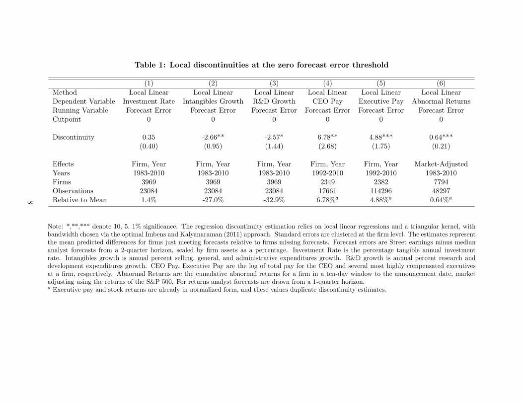
Table 1: Local discontinuities at the zero forecast error threshold

(1) (2) (3) (4) (5) (6)Method Local Linear Local Linear Local Linear Local Linear Local Linear Local LinearDependent Variable Investment Rate Intangibles Growth R&D Growth CEO Pay Executive Pay Abnormal ReturnsRunning Variable Forecast Error Forecast Error Forecast Error Forecast Error Forecast Error Forecast ErrorCutpoint 0 0 0 0 0 0

Discontinuity 0.35 -2.66** -2.57* 6.78** 4.88*** 0.64***(0.40) (0.95) (1.44) (2.68) (1.75) (0.21)

E↵ects Firm, Year Firm, Year Firm, Year Firm, Year Firm, Year Market-AdjustedYears 1983-2010 1983-2010 1983-2010 1992-2010 1992-2010 1983-2010Firms 3969 3969 3969 2349 2382 7794Observations 23084 23084 23084 17661 114296 48297Relative to Mean 1.4% -27.0% -32.9% 6.78%a 4.88%a 0.64%a

Note: *,**,*** denote 10, 5, 1% significance. The regression discontinuity estimation relies on local linear regressions and a triangular kernel, withbandwidth chosen via the optimal Imbens and Kalyanaraman (2011) approach. Standard errors are clustered at the firm level. The estimates representthe mean predicted di↵erences for firms just meeting forecasts relative to firms missing forecasts. Forecast errors are Street earnings minus mediananalyst forecasts from a 2-quarter horizon, scaled by firm assets as a percentage. Investment Rate is the percentage tangible annual investmentrate. Intangibles growth is annual percent selling, general, and administrative expenditures growth. R&D growth is annual percent research anddevelopment expenditures growth. CEO Pay, Executive Pay are the log of total pay for the CEO and several most highly compensated executivesat a firm, respectively. Abnormal Returns are the cumulative abnormal returns for a firm in a ten-day window to the announcement date, marketadjusting using the returns of the S&P 500. For returns analyst forecasts are drawn from a 1-quarter horizon.a Executive pay and stock returns are already in normalized form, and these values duplicate discontinuity estimates.

8

−6−4

−20

24

6

Intangibles Growth

YearPe

rcen

t Diff

eren

ce

0 1 2

−6−4

−20

24

6

R&D Growth

Year

0 1 2

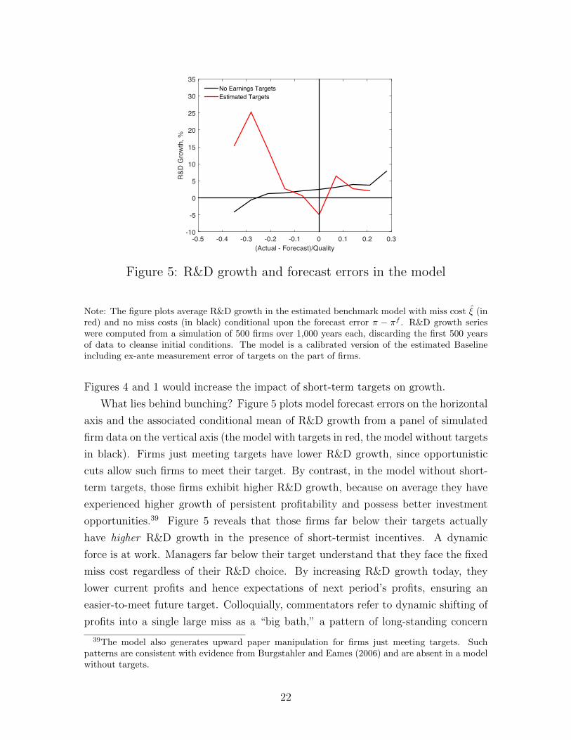
Figure 2: R&D growth dynamics in the data

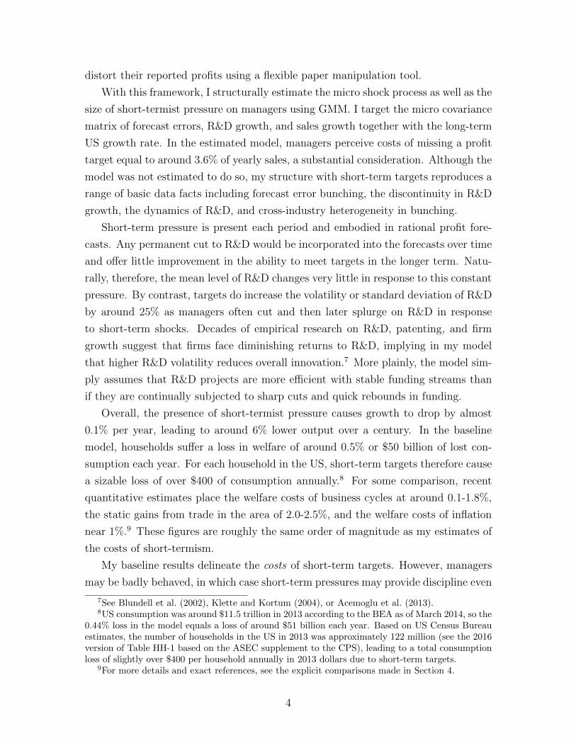
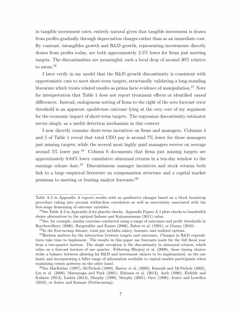
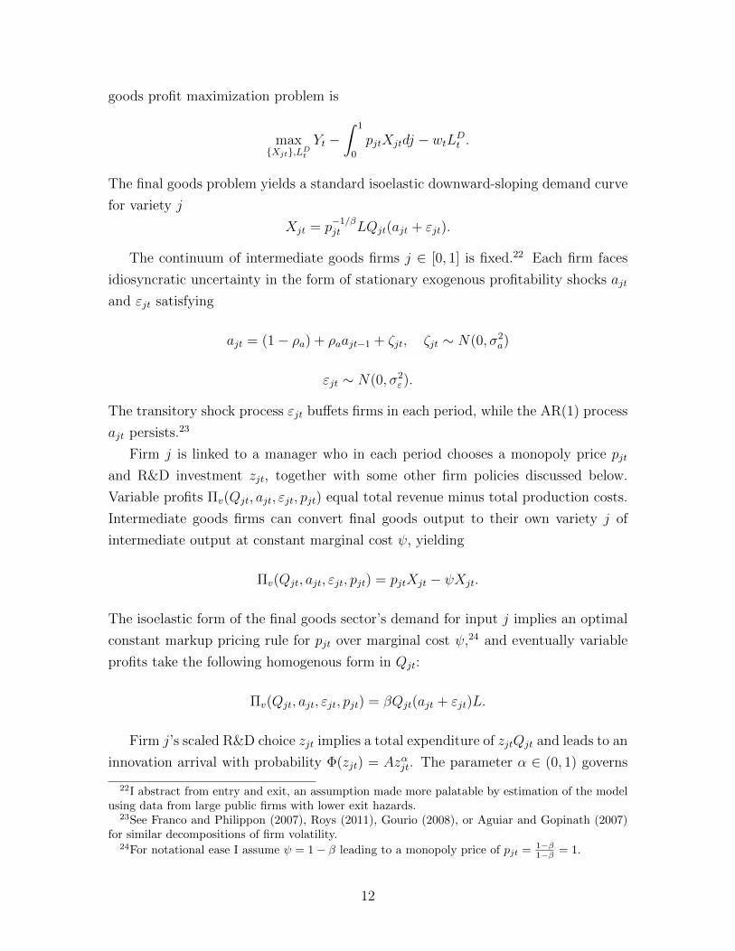
Note: The solid line is the discontinuity in long-term investment growth for firms just meetingrelative to just missing analyst forecasts. Year k on the horizontal axis reports estimates based onthe growth of long-term investment in the year t+ k with forecasts from year t. Intangibles growthand R&D growth are the annual percentage growth rate in selling, general, and administrativeexpenditures and research and development expenditures, respectively. The estimates are locally andnonparametrically computed using a local linear regression discontinuity estimator with bandwidthchosen according to the Imbens and Kalyanaraman (2011) approach. The running variables isforecast error or Street earnings minus median analyst forecasts from a 2-quarter horizon, scaledby firm assets as a percentage. Standard errors are clustered at the firm level, with 90% pointwiseconfidence intervals plotted in dashed lines. Sample drawn from the baseline Compustat-I/B/E/Sdiscontinuity estimation sample with 23,083 firm-years spanning 1983-2010 with 3,969 firms.

I now compare long-term investment behavior in future years t + k for firms

just meeting relative to just missing in year t. Figure 2 plots results for intangibles

growth in the left panel and R&D growth on the right. In the period in which firms

just meet a profit target, their long-term investment growth is lower, replicating

Table 1. However, by two years onwards, long-term investment growth exhibits a

reversal and overshoot. These dynamics place strong discipline on the channel through

which targets may impact R&D e�ciency, suggesting that volatility channels are more

plausible than persistent level e↵ects.

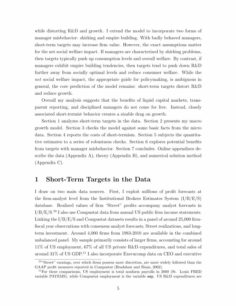
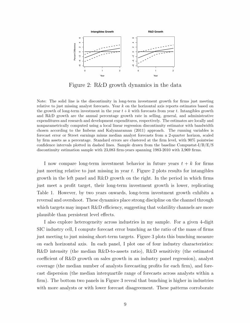
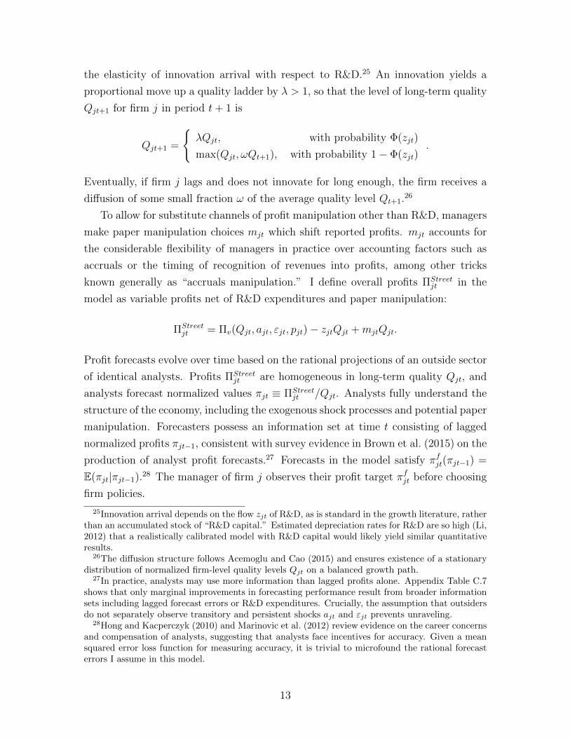
I also explore heterogeneity across industries in my sample. For a given 4-digit

SIC industry cell, I compute forecast error bunching as the ratio of the mass of firms

just meeting to just missing short-term targets. Figure 3 plots this bunching measure

on each horizontal axis. In each panel, I plot one of four industry characteristics:

R&D intensity (the median R&D-to-assets ratio), R&D sensitivity (the estimated

coe�cient of R&D growth on sales growth in an industry panel regression), analyst

coverage (the median number of analysts forecasting profits for each firm), and fore-

cast dispersion (the median interquartile range of forecasts across analysts within a

firm). The bottom two panels in Figure 3 reveal that bunching is higher in industries

with more analysts or with lower forecast disagreement. These patterns corroborate

9

●●

●

●●

●●

●

●

●

●

●

●●

●

0 20 40 60 80

0.0

0.2

0.4

0.6

R&D Sensitivity

R&D

to S

ales

, Ela

stic

ity

Slope = 0.003, R^2 = 0.16

●

●

●

●

●

●

●

●●

●

●

●

●

●

●

0 20 40 60 80

02

46

810

12

R&D Intensity

R&D

/ As

sets

, Per

cent

Slope = 0.06, R^2 = 0.21

●

●

●

●

●

●

●

●●● ●

●

●

●

●

0 20 40 60 80

34

56

78

9

Analyst Coverage

P(Just Meet) / P(Just Miss)

Num

ber o

f Ana

lyst

s

Slope = 0.016, R^2 = 0.078

●

●

●

● ●

●

●

●

●

●

●

●● ●●

0 20 40 60 80

1.5

2.5

3.5

4.5

Forecast Dispersion

P(Just Meet) / P(Just Miss)In

terq

uarti

le R

ange

, Per

cent

Slope = −0.01, R^2 = 0.085

Figure 3: Bunching varies across industries

Note: Horizontal axis is the ratio of firm-years just meeting to just missing forecasts in a 4-digit SICindustry cell, based on a 0.05% bandwidth relative to firm assets. Top left panel is the empiricalelasticity � from estimates of (R&D Growth)jt = � (Sales Growth)jt + fj + gt + "jt. Top rightpanel is the median R&D to assets ratio. Bottom left panel is the median number of analysts perfirm. Bottom right panel is the median interquartile range of analyst forecasts, relative to firmassets. Sample based on the baseline Compustat-I/B/E/S estimation sample with 23,083 firm-yearsspanning 1983-2010. Fitted lines, slopes, and R2’s included for reference.

evidence from Stein and Wang (2014), which rationalizes them in the context of a

time-varying uncertainty model. Turning to R&D, the top right panel documents

that industries with higher R&D intensity, and hence larger R&D budgets ripe for

manipulation, tend to bunch more. Finally, in the top left panel, industries with

higher R&D sensitivity to sales growth exhibit more bunching. My notion of R&D

sensitivity links to a long empirical tradition of computing the observed sensitivity of

firm-level investment to cash flows as well as conceptually to prior work by Barlevy

(2007) documenting R&D sensitivity to business cycles.21 I return later to examine

the equilibrium cross-sectional links between bunching and both R&D intensity and

R&D sensitivity in my model.

21See, for example, Fazzari et al. (1988), Gilchrist and Himmelberg (1995), Kaplan and Zingales(1997). A second strand of papers (Borisova and Brown, 2013; Brown et al., 2009; Brown andPetersen, 2009; Himmelberg and Petersen, 1994; Mairesse et al., 1999) studies R&D investmentrather than tangible investment.

10

The micro evidence in this section is consistent with systematic pressure on man-

agers to meet short-term profit targets and opportunistic manipulation of R&D. How-

ever suggestive or suspicious, such empirical patterns are mostly silent on questions

of aggregate impact, which I now consider in a quantitative model.

2 A Model of Short-Termist Incentives & Growth

In this section I present a quantitative model of macro growth and short-term profit

targets, followed by a discussion of the equilibrium concept, numerical solution method,

and structural estimation of the model.

Time is discrete, and a representative household subject to no aggregate uncer-

tainty maximizes utility from a flow of aggregate consumption Ct denominated in

units of a numeraire final good. Utility takes a standard constant relative risk aver-

sion form with subjective discount rate ⇢ and intertemporal elasticity of substitution1

�. The household purchases shares Sjt at price Pjt, receives dividends Djt from a fixed

continuum of intermediate goods firms j 2 [0, 1], inelastically supplies labor L to a

final goods sector at wage rate wt, and makes a savings choice Bt+1

in a one-period

bond with interest rate Rt+1

. The household problem is

maxCt,Bt+1,{Sjt}

1X

t=0

⇢

t C1��t

1� �

Ct +Bt+1

+

Z

1

0

PjtSjtdj = RtBt + wtL+

Z

1

0

(Pjt +Djt)Sjt�1

dj.

There are both intermediate and final goods sectors. The final good is produced in

a competitive constant returns to scale environment demanding intermediate goods

Xjt from each intermediate firm j and demanding labor in the amount LDt to produce

output Yt in each period. The labor share is �, and the final goods technology, broadly

following Acemoglu and Cao (2015), is given by

Yt =L

Dt�

(1� �)

Z

1

0

[Qjt(ajt + "jt)]�X

1��jt dj.

Each intermediate goods firm j at time t has a quality level Qjt. As discussed in more

detail below, each firm faces an exogenous profitability shock ajt + "jt made up of a

persistent component ajt and a transitory component "jt. Together, these determine

the marginal product of intermediate input Xjt in final goods production. The final

11

goods profit maximization problem is

max{Xjt},LD

t

Yt �Z

1

0

pjtXjtdj � wtLDt .

The final goods problem yields a standard isoelastic downward-sloping demand curve

for variety j

Xjt = p

�1/�jt LQjt(ajt + "jt).

The continuum of intermediate goods firms j 2 [0, 1] is fixed.22 Each firm faces

idiosyncratic uncertainty in the form of stationary exogenous profitability shocks ajt

and "jt satisfying

ajt = (1� ⇢a) + ⇢aajt�1

+ ⇣jt, ⇣jt ⇠ N(0, �2

a)

"jt ⇠ N(0, �2

").

The transitory shock process "jt bu↵ets firms in each period, while the AR(1) process

ajt persists.23

Firm j is linked to a manager who in each period chooses a monopoly price pjt

and R&D investment zjt, together with some other firm policies discussed below.

Variable profits ⇧v(Qjt, ajt, "jt, pjt) equal total revenue minus total production costs.

Intermediate goods firms can convert final goods output to their own variety j of

intermediate output at constant marginal cost , yielding

⇧v(Qjt, ajt, "jt, pjt) = pjtXjt � Xjt.

The isoelastic form of the final goods sector’s demand for input j implies an optimal

constant markup pricing rule for pjt over marginal cost ,24 and eventually variable

profits take the following homogenous form in Qjt:

⇧v(Qjt, ajt, "jt, pjt) = �Qjt(ajt + "jt)L.

Firm j’s scaled R&D choice zjt implies a total expenditure of zjtQjt and leads to an

innovation arrival with probability �(zjt) = Az

↵jt. The parameter ↵ 2 (0, 1) governs

22I abstract from entry and exit, an assumption made more palatable by estimation of the modelusing data from large public firms with lower exit hazards.

23See Franco and Philippon (2007), Roys (2011), Gourio (2008), or Aguiar and Gopinath (2007)for similar decompositions of firm volatility.

24For notational ease I assume = 1� � leading to a monopoly price of pjt =1��1�� = 1.

12

the elasticity of innovation arrival with respect to R&D.25 An innovation yields a

proportional move up a quality ladder by � > 1, so that the level of long-term quality

Qjt+1

for firm j in period t+ 1 is

Qjt+1

=

(

�Qjt, with probability �(zjt)

max(Qjt,!Qt+1

), with probability 1� �(zjt).

Eventually, if firm j lags and does not innovate for long enough, the firm receives a

di↵usion of some small fraction ! of the average quality level Qt+1

.26

To allow for substitute channels of profit manipulation other than R&D, managers

make paper manipulation choices mjt which shift reported profits. mjt accounts for

the considerable flexibility of managers in practice over accounting factors such as

accruals or the timing of recognition of revenues into profits, among other tricks

known generally as “accruals manipulation.” I define overall profits ⇧Streetjt in the

model as variable profits net of R&D expenditures and paper manipulation:

⇧Streetjt = ⇧v(Qjt, ajt, "jt, pjt)� zjtQjt +mjtQjt.

Profit forecasts evolve over time based on the rational projections of an outside sector

of identical analysts. Profits ⇧Streetjt are homogeneous in long-term quality Qjt, and

analysts forecast normalized values ⇡jt ⌘ ⇧Streetjt /Qjt. Analysts fully understand the

structure of the economy, including the exogenous shock processes and potential paper

manipulation. Forecasters possess an information set at time t consisting of lagged

normalized profits ⇡jt�1

, consistent with survey evidence in Brown et al. (2015) on the

production of analyst profit forecasts.27 Forecasts in the model satisfy ⇡fjt(⇡jt�1

) =

E(⇡jt|⇡jt�1

).28 The manager of firm j observes their profit target ⇡fjt before choosing

firm policies.

25Innovation arrival depends on the flow zjt of R&D, as is standard in the growth literature, ratherthan an accumulated stock of “R&D capital.” Estimated depreciation rates for R&D are so high (Li,2012) that a realistically calibrated model with R&D capital would likely yield similar quantitativeresults.

26The di↵usion structure follows Acemoglu and Cao (2015) and ensures existence of a stationarydistribution of normalized firm-level quality levels Qjt on a balanced growth path.

27In practice, analysts may use more information than lagged profits alone. Appendix Table C.7shows that only marginal improvements in forecasting performance result from broader informationsets including lagged forecast errors or R&D expenditures. Crucially, the assumption that outsidersdo not separately observe transitory and persistent shocks ajt and "jt prevents unraveling.

28Hong and Kacperczyk (2010) and Marinovic et al. (2012) review evidence on the career concernsand compensation of analysts, suggesting that analysts face incentives for accuracy. Given a meansquared error loss function for measuring accuracy, it is trivial to microfound the rational forecasterrors I assume in this model.

13

The manager of firm j maximizes the expected discounted flow of their personal

utility, solving29

max{zjt,mjt,pjt}t

E( 1X

t=0

✓

1

R

◆t

D

Mjt

)

.

Given manager choices for R&D, paper manipulation, and pricing, manager flow

utility is

D

Mjt = ✓dDjt � ⇠I(⇧Street

jt < ⇧fjt)Qjt.

The first term in D

Mjt is the manager’s share of dividends Djt, with an exogenous

ownership fraction ✓d in their firm. The second term encapsulates the impact of

short-term profit targets on incentives. A manager missing their profit target su↵ers

an exogenous fixed loss governed by the parameter ⇠ � 0. Firm dividends Djt in

period t equal variable profits minus R&D expenditures and some costs of paper

manipulation:

Djt = ⇧v(Qjt, ajt, "jt, pjt)� zjtQjt � �mm2

jtQjt.

The final term in dividends Djt is a quadratic cost of paper manipulation, stand-

ing in for some manager attention costs, higher auditor expenses, or even increased

probability of detection by outsiders implied by higher levels of profit manipulation.30

When target miss costs satisfy ⇠ = 0 the manager problem nests pure firm value

maximization. Note that the discontinuous, fixed nature of the miss cost is a natural

choice given forecast error bunching. In general, I allow for manager miss costs to be

purely private costs, firm resource costs, or manager pay cuts ⇠ = ⇠

manager+✓d⇠firm+

(1�✓d)⇠pay. The first component, ⇠manager, is purely private and could include manager

reputational concerns or costs of disrupted communication with outsiders which loom

large in practice (Dichev et al., 2013; Yermack and Li, 2014). The second term, ⇠firm,

a↵ects managers through the ownership share ✓d and reflects any resource, disruption,

or other costs borne by firms directly upon missing a target. Surveyed managers

report that avoiding target misses helps maintain low-cost external finance, avoids

triggering debt covenants, and even avoids costly shareholder litigation (Graham

et al., 2005). On the theoretical side, Stein (1989) notes that a desire to maintain

favorable costs of external finance may become self-reinforcing in the presence of short-

term pressure. The third and final component, ⇠pay, represents the potential for a firm

29On the balanced growth path which I will consider in this paper, interest rates are constant atan equilibrium value R allowing me to drop the subscript for interest rates Rt.

30See Dichev et al. (2013), Zakolyukina (2013), or Sun (2014) for further discussion of profit manip-ulation and its costs. Also, note that mjt could be trivially re-interpreted as forecast manipulationrather than profit manipulation.

14

to explicitly condition manager pay on targets. If pay includes not only a dividend

share but also an amount ⇠payQjt clawed back conditional upon a miss, the net loss

to a manager is (1 � ✓d)⇠pay. The evidence in Section 1 suggests that total pay is

discontinuously lower for managers just missing targets. My estimation strategy only

identifies the combined cost ⇠ rather than the three individual components ⇠manager,

⇠

firm, and ⇠pay. When making quantitative statements about the costs of targets, I

generally assume that the entirety of the term ⇠ represents personal costs ⇠manager.

This conservative approach implies that any change in aggregates stems from distorted

policies rather than mechanical resource costs.

The model admits a balanced growth path equilibrium in which all aggregates,

including average quality Qt =R

1

0

Qjtdj, grow at constant rate g. Appendix B de-

fines the equilibrium, which involves four major components: 1) optimal household

consumption and savings decisions Ct, Sjt, and Bt+1

given the budget constraint, 2)

competitive final goods firm optimization over intermediate goods Xjt and labor de-

mand L

Dt , 3) manager optimization over monopoly pricing pjt, R&D investment zjt,

and paper manipulation mjt, and 4) rational analyst forecasts ⇡fjt for each firm. An

economy-wide resource constraint, labor market clearing, asset market clearing, and

aggregate consistency conditions complete the definition.

I normalize the manager dynamic problem by the average quality levelQt to obtain

a stationary recursive formulation in Appendix B as a function of four state variables:

q (normalized endogenous long-term quality), a (exogenous persistent profitability),

" (exogenous transitory profitability), and ⇡f (endogenous analyst forecasts). I nota-

tionally omit dependence on j or t for readability, indicating future and lagged values

by 0 and �1

, respectively. I solve the manager problem using standard numerical dy-

namic programming techniques. I also rely upon a polynomial approximation to the

analyst expectation ⇡f = E(⇡|⇡�1

).31 For a given parameterization of the model and

solution to the manager’s problem, I compute a stationary distribution µ(q, a, ", ⇡f )

of firm states. Model aggregates are a function of the stationary distribution µ. My

solution method, explained in detail in Appendix C, involves a hybrid dampened

fixed-point and bisection algorithm iterating over the growth rate g, interest rate R,

and forecast function ⇡f (⇡�1

) such that the following three conditions hold:

1. The constant interest rate R and growth rate g satisfy the household Euler

equation R = 1

⇢(1 + g)�.

31Table C.7 in Appendix C records forecast accuracy statistics with alternative forecast systemsusing higher order approximations in ⇡�1 above the baseline linear rule. In all cases, the higher-orderapproximations yield little quantitative gain in forecast accuracy.

15

Table 2: Outside calibration of common parameters

Parameter Explanation Source, Value� CRRA Hall (2009), 2.0⇢ Discount rate Annual interest rate ⇡ 6%, 0.98� Labor share NIPA, 0.67L Human capital scale Normalization, 1.0↵ R&D curvature Blundell et al. (2002), 0.5� Quality step 25% increment, 1.25! Quality di↵usion boundary Normalization, 0.08✓d Manager equity share Nikolov and Whited (2014), 5.1%

Note: The table displays the notation (first column) as well as an explanation (second column) ofeach model parameter fixed by outside calibration. The third column lists the source and value ofeach common parameter.

2. The growth rate g results from aggregation of R&D policies z and the innovation

arrival function �(z) over the stationary distribution µ.32

3. Analyst profit forecasts are rational given the equilibrium distribution µ, i.e.

⇡

f = Eµ(⇡|⇡�1

).

Numerical analysis of the baseline model requires fixing the values of many param-

eters. For the most part I follow a structural estimation strategy based on GMM using

firm-level moments from my joint sample of Compustat and I/B/E/S data. However,

before estimating the model I externally calibrate some parameters reported in Table

2.

The model period is one year. An intertemporal elasticity of substitution of 0.5

or � = 2, a subjective discount rate of ⇢ = 1/1.02 ⇡ 0.98, and a targeted growth

rate of near 2% yield annual interest rates of around 6%. A labor share of � = 2/3

matches standard values in the quantitative macro literature, and a value of � = 1.25

implies long-term quality increases of 25% upon innovation arrival.33 The di↵usion

boundary ! determines the lower endpoint of the state space in relative quality q.

I choose its value so that in my numerical solution the ratio between the highest

and lowest quality levels for firms is normalized to the round figure of 150, requiring

! = 1p150

⇡ 0.08.34 I normalize labor supply to L = 1, and choose a manager equity

32See Appendix B equation (1) for the exact statement of this condition.33I fix quality step size at the round value of 25%. Structural estimates of the quality step size

from Peters (2013) or Acemoglu et al. (2013) would suggest values on the order of 7-14% instead. Asshown in Appendix Table C.6, my choice of a higher, round value for � is unimportant for growthand welfare statements.

34Naturally, this requires that the upper endpoint for relative quality in my numerical solution is

16

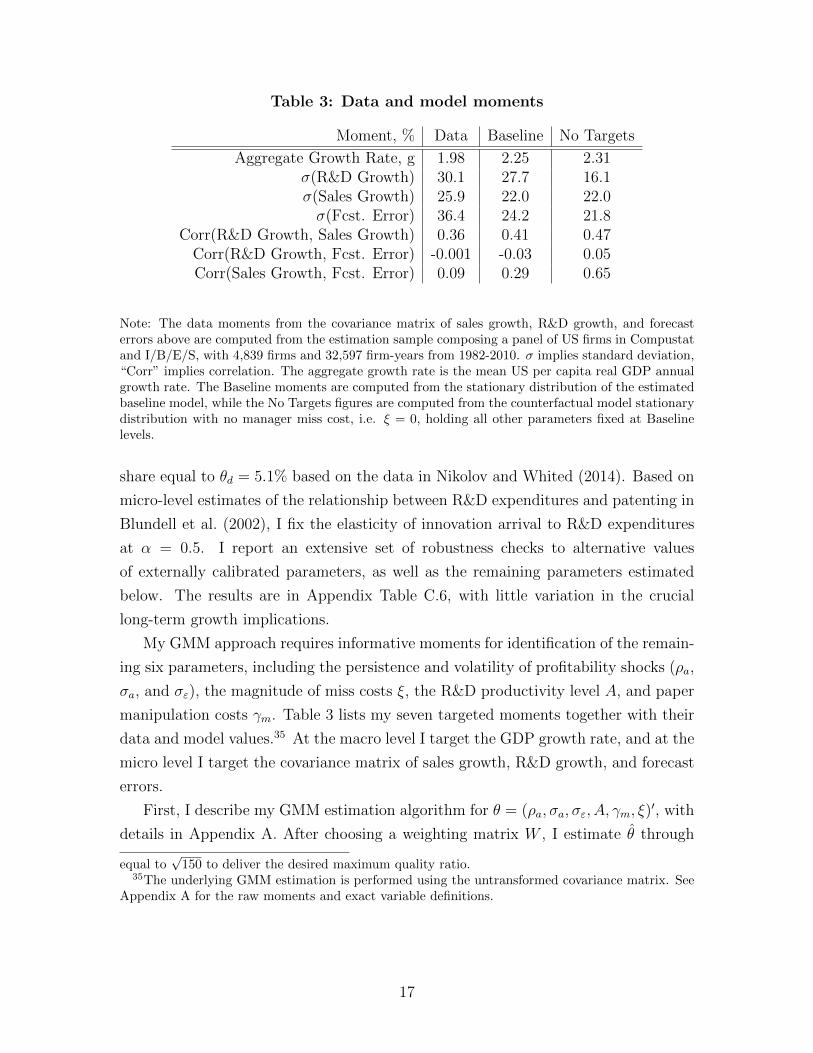
Table 3: Data and model moments

Moment, % Data Baseline No Targets

Aggregate Growth Rate, g 1.98 2.25 2.31�(R&D Growth) 30.1 27.7 16.1�(Sales Growth) 25.9 22.0 22.0�(Fcst. Error) 36.4 24.2 21.8

Corr(R&D Growth, Sales Growth) 0.36 0.41 0.47Corr(R&D Growth, Fcst. Error) -0.001 -0.03 0.05Corr(Sales Growth, Fcst. Error) 0.09 0.29 0.65

Note: The data moments from the covariance matrix of sales growth, R&D growth, and forecasterrors above are computed from the estimation sample composing a panel of US firms in Compustatand I/B/E/S, with 4,839 firms and 32,597 firm-years from 1982-2010. � implies standard deviation,“Corr” implies correlation. The aggregate growth rate is the mean US per capita real GDP annualgrowth rate. The Baseline moments are computed from the stationary distribution of the estimatedbaseline model, while the No Targets figures are computed from the counterfactual model stationarydistribution with no manager miss cost, i.e. ⇠ = 0, holding all other parameters fixed at Baselinelevels.

share equal to ✓d = 5.1% based on the data in Nikolov and Whited (2014). Based on

micro-level estimates of the relationship between R&D expenditures and patenting in

Blundell et al. (2002), I fix the elasticity of innovation arrival to R&D expenditures

at ↵ = 0.5. I report an extensive set of robustness checks to alternative values

of externally calibrated parameters, as well as the remaining parameters estimated

below. The results are in Appendix Table C.6, with little variation in the crucial

long-term growth implications.

My GMM approach requires informative moments for identification of the remain-

ing six parameters, including the persistence and volatility of profitability shocks (⇢a,

�a, and �"), the magnitude of miss costs ⇠, the R&D productivity level A, and paper

manipulation costs �m. Table 3 lists my seven targeted moments together with their

data and model values.35 At the macro level I target the GDP growth rate, and at the

micro level I target the covariance matrix of sales growth, R&D growth, and forecast

errors.

First, I describe my GMM estimation algorithm for ✓ = (⇢a, �a, �", A, �m, ⇠)0, with

details in Appendix A. After choosing a weighting matrix W , I estimate ✓ through

equal top150 to deliver the desired maximum quality ratio.

35The underlying GMM estimation is performed using the untransformed covariance matrix. SeeAppendix A for the raw moments and exact variable definitions.

17

numerical minimization

✓ = argmin✓

[m(✓)�m(X)]0 W [m(✓)�m(X)] ,

where m(X) and m(✓) are the vector of moments from the data X and model with

parameters ✓, respectively. The moment weighting matrix W I use results in a sum

of squared percentage deviations objective, a natural scale-free alternative to the

asymptotically e�cient GMM weighting matrix which often su↵ers from finite-sample

bias (Altonji and Segal, 1996).

The mapping between moments and estimated parameters in the model is joint

and not one-to-one. However, certain moments are particularly influential for the

identification of a given parameter. I investigate this mapping by computing Gentzkow

and Shapiro (2014) sensitivity statistics as reported in Appendix Figure C.5. These

sensitivity measures represent the estimated coe�cients of a theoretical regression of

parameters on model moments over their joint asymptotic distribution. The R&D

productivity parameter A depends heavily on the aggregate growth rate, because

higher innovation arrival rates imply higher growth. Forward-looking R&D feeds into

realized forecast errors, implying that persistent shock volatility �a loads particularly

upon R&D growth as well as forecast error volatility. By contrast, the estimated tran-

sitory shock volatility �" depends relatively more upon overall sales growth volatility.

Estimation of the persistence ⇢a links to the behavior of forward-looking R&D, plac-

ing weight on each of the volatility moments in the data but also crucially on the

covariance between sales and R&D growth. Since easier paper manipulation in the

model dampens passthrough of sales growth to profits, the cost parameter �m is de-

termined in large part by the observed covariance between sales growth and forecast

errors. Finally, I show below that the primary manifestation of pressure from miss

costs ⇠ is higher R&D volatility, as firms sometimes react to shocks by cutting R&D

to boost profits above targets. Naturally, therefore, the estimated level of ⇠ depends

crucially upon both R&D growth volatility as well as the covariance between forecast

errors and R&D growth.

Table 4 reports the estimated parameters and standard errors. The persistent

component of profitability is highly autocorrelated, with ⇢a approximately equal to

0.9, and the combination of persistent and transitory volatility,p

�

2

a + �

2

" , is moder-

ate at around 12% annually. The persistence and volatility compare closely to the

parameters in both Gourio and Rudanko (2014) as well as Hennessy and Whited

(2007), which are also based on dynamic firm-level problems and Compustat data.

18

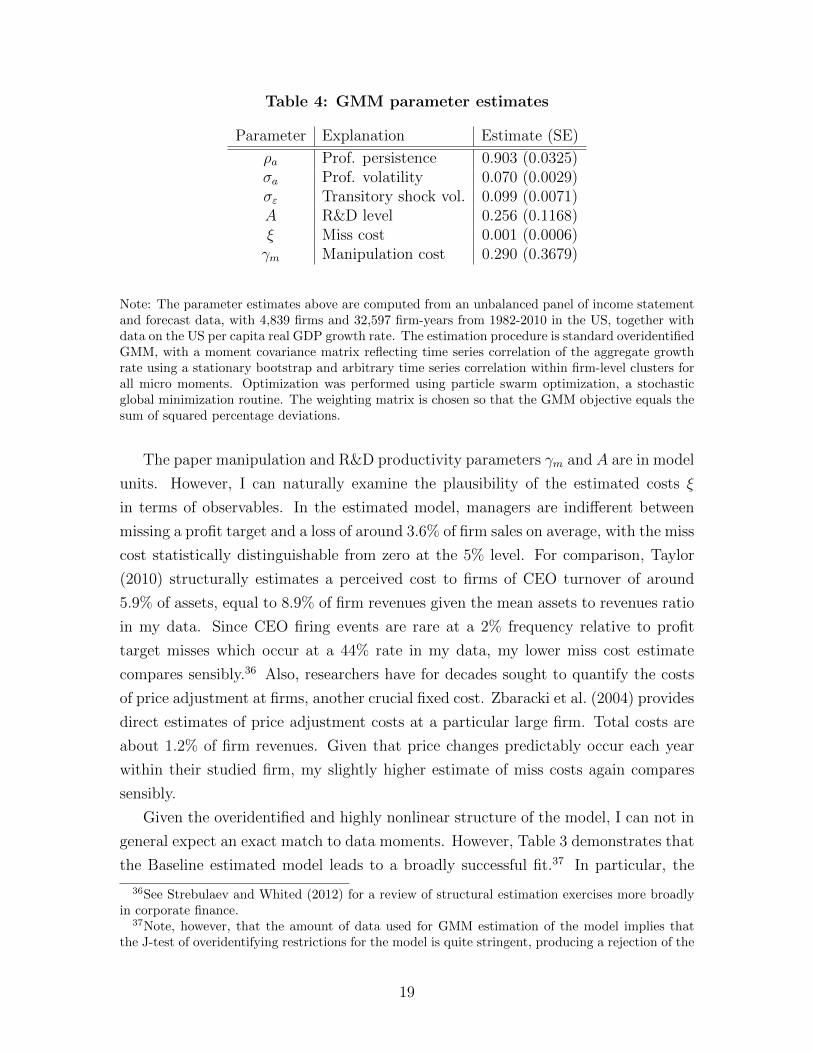
Table 4: GMM parameter estimates

Parameter Explanation Estimate (SE)

⇢a Prof. persistence 0.903 (0.0325)�a Prof. volatility 0.070 (0.0029)�" Transitory shock vol. 0.099 (0.0071)A R&D level 0.256 (0.1168)⇠ Miss cost 0.001 (0.0006)�m Manipulation cost 0.290 (0.3679)

Note: The parameter estimates above are computed from an unbalanced panel of income statementand forecast data, with 4,839 firms and 32,597 firm-years from 1982-2010 in the US, together withdata on the US per capita real GDP growth rate. The estimation procedure is standard overidentifiedGMM, with a moment covariance matrix reflecting time series correlation of the aggregate growthrate using a stationary bootstrap and arbitrary time series correlation within firm-level clusters forall micro moments. Optimization was performed using particle swarm optimization, a stochasticglobal minimization routine. The weighting matrix is chosen so that the GMM objective equals thesum of squared percentage deviations.

The paper manipulation and R&D productivity parameters �m and A are in model

units. However, I can naturally examine the plausibility of the estimated costs ⇠

in terms of observables. In the estimated model, managers are indi↵erent between

missing a profit target and a loss of around 3.6% of firm sales on average, with the miss

cost statistically distinguishable from zero at the 5% level. For comparison, Taylor

(2010) structurally estimates a perceived cost to firms of CEO turnover of around

5.9% of assets, equal to 8.9% of firm revenues given the mean assets to revenues ratio

in my data. Since CEO firing events are rare at a 2% frequency relative to profit

target misses which occur at a 44% rate in my data, my lower miss cost estimate

compares sensibly.36 Also, researchers have for decades sought to quantify the costs

of price adjustment at firms, another crucial fixed cost. Zbaracki et al. (2004) provides

direct estimates of price adjustment costs at a particular large firm. Total costs are

about 1.2% of firm revenues. Given that price changes predictably occur each year

within their studied firm, my slightly higher estimate of miss costs again compares

sensibly.

Given the overidentified and highly nonlinear structure of the model, I can not in

general expect an exact match to data moments. However, Table 3 demonstrates that

the Baseline estimated model leads to a broadly successful fit.37 In particular, the

36See Strebulaev and Whited (2012) for a review of structural estimation exercises more broadlyin corporate finance.

37Note, however, that the amount of data used for GMM estimation of the model implies thatthe J-test of overidentifying restrictions for the model is quite stringent, producing a rejection of the

19

Baseline delivers a growth rate around the 2% level in the data, together with sub-

stantial volatility in sales growth. The Baseline model delivers somewhat less volatile

forecast errors than the data, but higher volatility than a model without short-term

pressure (moments of this No Targets case with ⇠ = 0 are also reported in Table 3).

Furthermore, in both the Baseline and the data, forecast errors negatively covary with

R&D growth. Targets cause some cuts to R&D growth which are driven by a desire

to meet forecasts and are therefore correlated with higher forecast errors. By con-

trast, the No Targets model in which R&D responds only to investment opportunities

produces a positive correlation of forecast errors with R&D growth. The presence of

targets in the Baseline causes R&D to depend on transitory shocks, increasing the

volatility of R&D growth substantially, while the No Targets model underpredicts

R&D growth volatility by a large margin. Finally, paper manipulation in the Base-

line leads to lower correlation between sales growth and forecast errors, closer to the

data, while a No Targets model overpredicts this correlation substantially.

3 Assessing the Model

Along multiple dimensions - the cross-section of forecast errors, apparent opportunis-

tic cuts to R&D growth, the dynamics of R&D, and the cross-section of industry

heterogeneity - I show in this section that the estimated model delivers some basic

facts from the micro data. Recall that the single substantive departure from pure

value maximization in the model is the parsimonious introduction of the fixed cost ⇠,

and note that each of these patterns goes untargeted in my estimation.

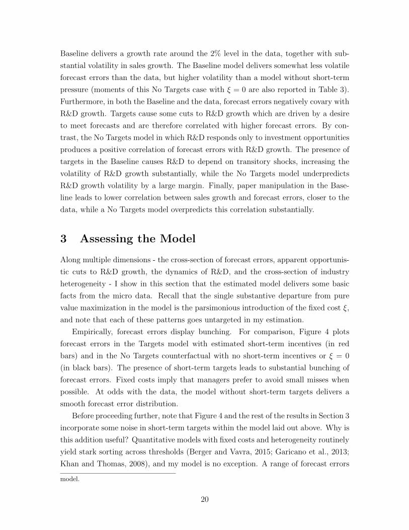
Empirically, forecast errors display bunching. For comparison, Figure 4 plots

forecast errors in the Targets model with estimated short-term incentives (in red

bars) and in the No Targets counterfactual with no short-term incentives or ⇠ = 0

(in black bars). The presence of short-term targets leads to substantial bunching of

forecast errors. Fixed costs imply that managers prefer to avoid small misses when

possible. At odds with the data, the model without short-term targets delivers a

smooth forecast error distribution.

Before proceeding further, note that Figure 4 and the rest of the results in Section 3

incorporate some noise in short-term targets within the model laid out above. Why is

this addition useful? Quantitative models with fixed costs and heterogeneity routinely

yield stark sorting across thresholds (Berger and Vavra, 2015; Garicano et al., 2013;

Khan and Thomas, 2008), and my model is no exception. A range of forecast errors

model.

20

−0.5 −0.4 −0.3 −0.2 −0.1 0 0.1 0.2 0.30

0.05

0.1

0.15

0.2

0.25

0.3

0.35

0.4

0.45

0.5

Forecast Error = (Actual − Forecast)/Quality

Den

sity

No Earnings TargetsEstimated Targets

Student Version of MATLAB

Figure 4: Forecast errors and bunching in the model

Note: The figure above represents the distribution of forecast errors ⇡ � ⇡f computed from thestationary distribution of the balanced growth path associated with the estimated miss cost ⇠ (inred) and the counterfactual ⇠ = 0 (in black). The model is a calibrated version of the estimatedBaseline including ex-ante measurement error of targets on the part of firms.

just below zero never occurs if measurement error is ignored. The literature routinely

incorporates some quantitative addition, such as measurement error or maintenance

investment depending on the context, in order to allow for looser sorting. Appendix B

lays out my extended model of manager decisions with a decomposition of transitory

profitability shocks into two separate components: "jt (known to managers when

policies are decided) and another component ⌫jt (unknown to managers when policies

are decided). In practice the noise ⌫jt serves as target measurement error, since the

exact threshold for meeting the target is ex-ante uncertain. Outside of Section 3,

in which direct comparison of firm outcomes to forecast errors is not the object

of interest, I discuss results generated by the Baseline model without noise. This

choice is not crucial but instead is conservative for my conclusions about the growth

impact of targets.38 Importantly, this logic also implies that my choice to target the

second moments of forecast errors, rather than the exact shape of the forecast error

distribution, is conservative as well. The additional noise required to explicitly match

38In particular, in the presence of noise more managers face a possible miss, causing a largeroverall growth reduction. Compare Table 6 to Appendix Table C.6 for exact di↵erences. Theanalogue to Figure 4 without measurement error is Appendix Figure C.4. Finally, note that forFigures 4-6, I calibrate the decomposition of known and unknown transitory shock volatilities toattribute approximately half of the total estimated transitory volatility to each source, since I drawprofit forecasts in the data from the middle of the fiscal year.

21

(Actual - Forecast)/Quality-0.5 -0.4 -0.3 -0.2 -0.1 0 0.1 0.2 0.3

R&D

Gro

wth

, %

-10

-5

0

5

10

15

20

25

30

35No Earnings TargetsEstimated Targets

Figure 5: R&D growth and forecast errors in the model

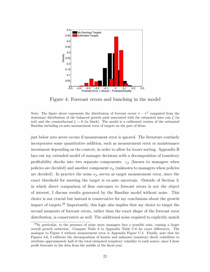
Note: The figure plots average R&D growth in the estimated benchmark model with miss cost ⇠ (inred) and no miss costs (in black) conditional upon the forecast error ⇡ � ⇡f . R&D growth serieswere computed from a simulation of 500 firms over 1,000 years each, discarding the first 500 yearsof data to cleanse initial conditions. The model is a calibrated version of the estimated Baselineincluding ex-ante measurement error of targets on the part of firms.

Figures 4 and 1 would increase the impact of short-term targets on growth.

What lies behind bunching? Figure 5 plots model forecast errors on the horizontal

axis and the associated conditional mean of R&D growth from a panel of simulated

firm data on the vertical axis (the model with targets in red, the model without targets

in black). Firms just meeting targets have lower R&D growth, since opportunistic

cuts allow such firms to meet their target. By contrast, in the model without short-

term targets, those firms exhibit higher R&D growth, because on average they have

experienced higher growth of persistent profitability and possess better investment

opportunities.39 Figure 5 reveals that those firms far below their targets actually

have higher R&D growth in the presence of short-termist incentives. A dynamic

force is at work. Managers far below their target understand that they face the fixed

miss cost regardless of their R&D choice. By increasing R&D growth today, they

lower current profits and hence expectations of next period’s profits, ensuring an

easier-to-meet future target. Colloquially, commentators refer to dynamic shifting of

profits into a single large miss as a “big bath,” a pattern of long-standing concern

39The model also generates upward paper manipulation for firms just meeting targets. Suchpatterns are consistent with evidence from Burgstahler and Eames (2006) and are absent in a modelwithout targets.

22

−6−4

−20

24

6

Data

YearR

&D G

row

th, %

Diff

eren

ce

0 1 2

−10

−50

510

Model

Year

0 1 2

No Earnings TargetsEstimated Targets

Figure 6: R&D growth dynamics in the data and the model

Note: Both panels plot in solid lines the estimated discontinuity in annual percentage R&D growthfor firms just meeting relative to just missing analyst forecasts. Year k on the horizontal axisreports estimates based on year t+ k R&D growth and year t forecasts. All estimates are computedusing a local linear regression discontinuity estimator, with a running variable equal to earningsforecast errors normalized by firm assets (data, bandwidth from Imbens and Kalyanaraman (2011))and firm quality q (model, bandwidth = 0.2). The data panel reports 90% pointwise confidenceintervals (dotted lines). The model panel reports estimates from the baseline model (in red, with⇠) and from the model with no earnings targets (in black, with ⇠ = 0). Data estimates rely onthe baseline Compustat-I/B/E/S discontinuity estimation sample with 23,083 firm-years spanning1983-2010 with 3,969 firms. Model estimates rely on simulation of 500 firms over 1,000 years each,discarding the first 500 years of data to cleanse initial conditions.

to Securities and Exchange Commission regulators.40 A model without short-termist

incentives fails to generate this dynamic profit shifting.

Firms in the data just meeting targets in year t have on average lower R&D

growth. However, Figure 2 from Section 1 reveals that in subsequent years such firms

have higher R&D growth. To investigate, I first replicate the dynamics from Figure

2 in the left panel of Figure 6. In the right panel I plot the results of an analogous

empirical exercise conducted with simulated model data. In the model I apply the

same regression discontinuity estimator to measure the average di↵erence in R&D

growth between firms just meeting and missing targets. Moving along the horizontal

axis, I trace out the di↵erence in subsequent years. The model with short-term targets

(the red line) exhibits lower R&D growth for firms just meeting targets. However,

two years in the future, R&D growth is higher for firms that just met targets today.

Opportunistic cuts and subsequent rebounds follow the pattern seen in Table 1 and

Figure 2 in the data. These rich dynamics are absent in the model without short-term

targets (the black line). What economic force is at work? In the model with short-

term incentives, firms just meeting targets due to opportunistic cuts have lower R&D,

relative to investment opportunities, than firms missing targets. Because they met

40See the remarks by the SEC chairman in Levitt (1998).

23

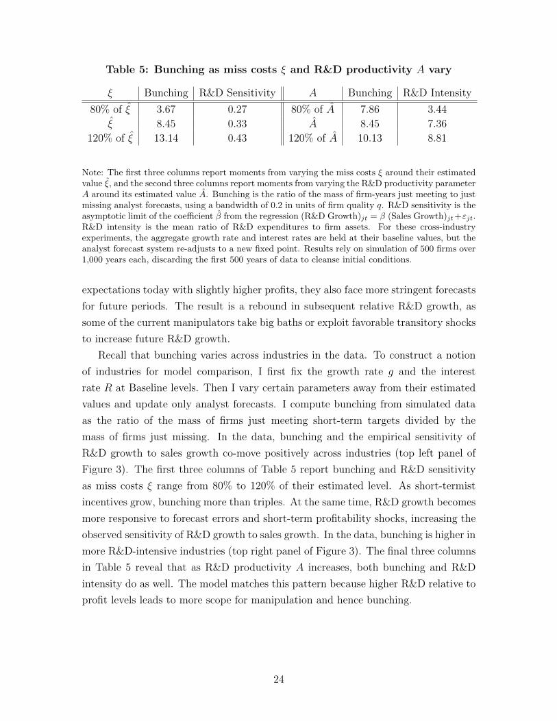
Table 5: Bunching as miss costs ⇠ and R&D productivity A vary

⇠ Bunching R&D Sensitivity A Bunching R&D Intensity

80% of ⇠ 3.67 0.27 80% of A 7.86 3.44⇠ 8.45 0.33 A 8.45 7.36

120% of ⇠ 13.14 0.43 120% of A 10.13 8.81

Note: The first three columns report moments from varying the miss costs ⇠ around their estimatedvalue ⇠, and the second three columns report moments from varying the R&D productivity parameterA around its estimated value A. Bunching is the ratio of the mass of firm-years just meeting to justmissing analyst forecasts, using a bandwidth of 0.2 in units of firm quality q. R&D sensitivity is theasymptotic limit of the coe�cient � from the regression (R&D Growth)jt = � (Sales Growth)jt+"jt.R&D intensity is the mean ratio of R&D expenditures to firm assets. For these cross-industryexperiments, the aggregate growth rate and interest rates are held at their baseline values, but theanalyst forecast system re-adjusts to a new fixed point. Results rely on simulation of 500 firms over1,000 years each, discarding the first 500 years of data to cleanse initial conditions.

expectations today with slightly higher profits, they also face more stringent forecasts

for future periods. The result is a rebound in subsequent relative R&D growth, as

some of the current manipulators take big baths or exploit favorable transitory shocks

to increase future R&D growth.

Recall that bunching varies across industries in the data. To construct a notion

of industries for model comparison, I first fix the growth rate g and the interest

rate R at Baseline levels. Then I vary certain parameters away from their estimated

values and update only analyst forecasts. I compute bunching from simulated data

as the ratio of the mass of firms just meeting short-term targets divided by the

mass of firms just missing. In the data, bunching and the empirical sensitivity of

R&D growth to sales growth co-move positively across industries (top left panel of

Figure 3). The first three columns of Table 5 report bunching and R&D sensitivity

as miss costs ⇠ range from 80% to 120% of their estimated level. As short-termist

incentives grow, bunching more than triples. At the same time, R&D growth becomes

more responsive to forecast errors and short-term profitability shocks, increasing the

observed sensitivity of R&D growth to sales growth. In the data, bunching is higher in

more R&D-intensive industries (top right panel of Figure 3). The final three columns

in Table 5 reveal that as R&D productivity A increases, both bunching and R&D

intensity do as well. The model matches this pattern because higher R&D relative to

profit levels leads to more scope for manipulation and hence bunching.

24

−0.15 −0.1 −0.05 0 0.05 0.1 0.1585

90

95

100

105

110

115

Mea

n R

&D (N

o Ta

rget

s =

100)

Transitory Shock ε

No TargetsEstimated Targets

Student Version of MATLAB

Figure 7: R&D and short-term shocks in the model

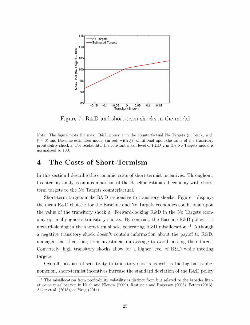
Note: The figure plots the mean R&D policy z in the counterfactual No Targets (in black, with⇠ = 0) and Baseline estimated model (in red, with ⇠) conditional upon the value of the transitoryprofitability shock ". For readability, the constant mean level of R&D z in the No Targets model isnormalized to 100.

4 The Costs of Short-Termism

In this section I describe the economic costs of short-termist incentives. Throughout,

I center my analysis on a comparison of the Baseline estimated economy with short-

term targets to the No Targets counterfactual.

Short-term targets make R&D responsive to transitory shocks. Figure 7 displays

the mean R&D choice z for the Baseline and No Targets economies conditional upon

the value of the transitory shock ". Forward-looking R&D in the No Targets econ-

omy optimally ignores transitory shocks. By contrast, the Baseline R&D policy z is

upward-sloping in the short-term shock, generating R&D misallocation.41 Although

a negative transitory shock doesn’t contain information about the payo↵ to R&D,

managers cut their long-term investment on average to avoid missing their target.

Conversely, high transitory shocks allow for a higher level of R&D while meeting

targets.

Overall, because of sensitivity to transitory shocks as well as the big baths phe-

nomenon, short-termist incentives increase the standard deviation of the R&D policy

41The misallocation from profitability volatility is distinct from but related to the broader liter-ature on misallocation in Hsieh and Klenow (2009), Restuccia and Rogerson (2008), Peters (2013),Asker et al. (2013), or Yang (2014).

25

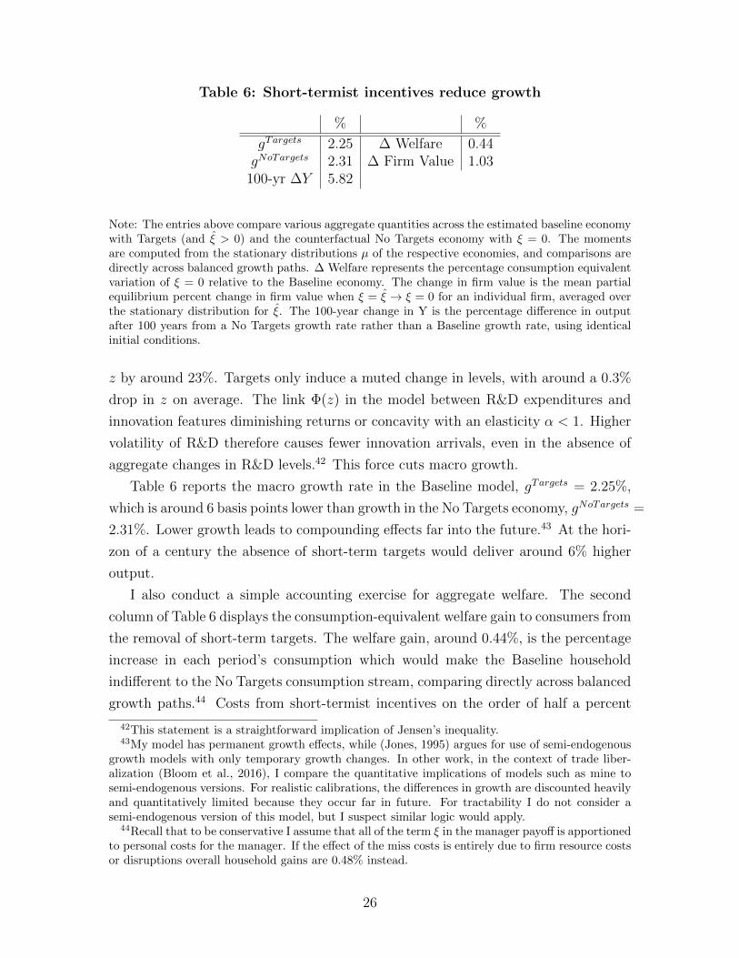
Table 6: Short-termist incentives reduce growth

% %

g

Targets 2.25 � Welfare 0.44g

NoTargets 2.31 � Firm Value 1.03100-yr �Y 5.82

Note: The entries above compare various aggregate quantities across the estimated baseline economywith Targets (and ⇠ > 0) and the counterfactual No Targets economy with ⇠ = 0. The momentsare computed from the stationary distributions µ of the respective economies, and comparisons aredirectly across balanced growth paths. � Welfare represents the percentage consumption equivalentvariation of ⇠ = 0 relative to the Baseline economy. The change in firm value is the mean partialequilibrium percent change in firm value when ⇠ = ⇠ ! ⇠ = 0 for an individual firm, averaged overthe stationary distribution for ⇠. The 100-year change in Y is the percentage di↵erence in outputafter 100 years from a No Targets growth rate rather than a Baseline growth rate, using identicalinitial conditions.

z by around 23%. Targets only induce a muted change in levels, with around a 0.3%

drop in z on average. The link �(z) in the model between R&D expenditures and

innovation features diminishing returns or concavity with an elasticity ↵ < 1. Higher

volatility of R&D therefore causes fewer innovation arrivals, even in the absence of

aggregate changes in R&D levels.42 This force cuts macro growth.

Table 6 reports the macro growth rate in the Baseline model, gTargets = 2.25%,

which is around 6 basis points lower than growth in the No Targets economy, gNoTargets =

2.31%. Lower growth leads to compounding e↵ects far into the future.43 At the hori-

zon of a century the absence of short-term targets would deliver around 6% higher

output.

I also conduct a simple accounting exercise for aggregate welfare. The second

column of Table 6 displays the consumption-equivalent welfare gain to consumers from

the removal of short-term targets. The welfare gain, around 0.44%, is the percentage

increase in each period’s consumption which would make the Baseline household

indi↵erent to the No Targets consumption stream, comparing directly across balanced

growth paths.44 Costs from short-termist incentives on the order of half a percent

42This statement is a straightforward implication of Jensen’s inequality.43My model has permanent growth e↵ects, while (Jones, 1995) argues for use of semi-endogenous

growth models with only temporary growth changes. In other work, in the context of trade liber-alization (Bloom et al., 2016), I compare the quantitative implications of models such as mine tosemi-endogenous versions. For realistic calibrations, the di↵erences in growth are discounted heavilyand quantitatively limited because they occur far in future. For tractability I do not consider asemi-endogenous version of this model, but I suspect similar logic would apply.

44Recall that to be conservative I assume that all of the term ⇠ in the manager payo↵ is apportionedto personal costs for the manager. If the e↵ect of the miss costs is entirely due to firm resource costsor disruptions overall household gains are 0.48% instead.

26

should be compared to other macro factors. Recent estimates of the welfare costs

of business cycles range from 0.1-1.8% (Krusell et al., 2009), and recent estimates

of the static gains from trade range from 2.0-2.5% (Costinot and Rodrıguez-Clare,

2015; Melitz and Redding, 2013).45 At the macro level, the quantitative costs due to

short-termist targets are sizable.

Table 6 also reports the change in average firm value resulting in partial equi-

librium from the removal of targets, equal to around 1%.46 For perspective, I turn

to evidence from corporate finance quantifying the loss in value from CEO turnover

frictions at around 3% (Taylor, 2010) or from manager agency frictions a↵ecting cash

holding at around 6% (Nikolov and Whited, 2014). At the micro level, the quantita-

tive costs of short-term targets also appear sizable.

Note that my counterfactual exercise assumes that US public firms, representing

around two-thirds of all private R&D expenditures, are a reasonable proxy for all

US firms. On one hand, private firms are not typically subject to profit reporting

requirements or to analyst forecasts. However, on the other hand, private-firm exec-

utives surveyed in Graham et al. (2005) report almost identical levels of pressure to

meet profit targets as their public-firm counterparts. For private firms, profit targets

are presumably internal, stemming from monitoring or goals set by boards or private

investors. On net, it is not clear ex-ante whether private firms are more or less insu-

lated from short-termist pressures.47 However, if private firms are indeed less subject

to short-termist pressures, their decision to publicly list may be distorted, potentially

leading to heightened financial frictions in the economy with targets. The comparison

seems rich, but a fuller treatment remains beyond the scope of this paper.

5 Quantitative Robustness and Discussion

Quantitative statements require careful defense. In this section, I first explore a

range of parameterizations of my model, asking whether the costs of short-termist

incentives fall away under plausible alternative cases. Then, I narrow my discussion

to two parameters: the elasticity of innovation with respect to R&D expenditures

(↵) and the costs of paper manipulation (�m). In both cases, I discuss the empirical

45For more perspective on the magnitude of welfare losses here, see Hassan and Mertens (2011) forthe social cost of “near-rationality” in investment, around 2.4% in consumption-equivalent terms,or see the broader discussion of the costs of business cycles in Lucas (2003)

46For conservatism I assume miss costs are private to the manager. If miss costs are borne asresource costs to the firm, the change in firm value is 1.3%.

47However, see recent empirical work on this topic by Bernstein (2015), Asker et al. (2014), andAghion et al. (2013).

27

0 0.05 0.1 0.15Percent Change in Growth

Alte

rnat

ive

Cas

es

Baseline

Lower ρa

Higher ρa

Lower σa

Higher σa

Lower σε

Higher σε

Lower AHigher A

Lower ξHigher ξ

Lower γm

Higher γm

Infinite γm

Lower ⍺Higher ⍺

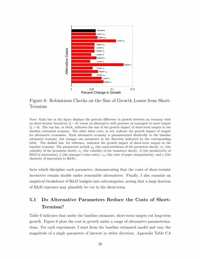
Figure 8: Robustness Checks on the Size of Growth Losses from Short-Termism

Note: Each bar in the figure displays the percent di↵erence in growth between an economy withno short-termist incentives (⇠ = 0) versus an alternative with pressure on managers to meet targets(⇠ > 0). The top bar, in black, indicates the size of the growth impact of short-term targets in thebaseline estimated economy. The other lower rows, in red, indicate the growth impact of targetsfor alternative economies. Each alternative economy is parameterized identically to the baselineestimated economy, but changes one parameter in the direction indicated by the correspondinglabel. The dashed line, for reference, indicates the growth impact of short-term targets in thebaseline economy. The parameters include ⇢a (the autocorrelation of the persistent shock), �a (thevolatility of the persistent shock), �" (the volatility of the transitory shock), A (the productivity ofR&D in innovation), ⇠ (the manager’s miss costs), �m (the costs of paper manipulation), and ↵ (theelasticity of innovation to R&D).

facts which discipline each parameter, demonstrating that the costs of short-termist

incentives remain sizable under reasonable alternatives. Finally, I also examine an

empirical breakdown of R&D budgets into subcategories, noting that a large fraction

of R&D expenses may plausibly be cut in the short-term.

5.1 Do Alternative Parameters Reduce the Costs of Short-

Termism?

Table 6 indicates that under the baseline estimates, short-term targets cut long-term

growth. Figure 8 plots the cost in growth under a range of alternative parameteriza-

tions. For each experiment, I start from the baseline estimated model and vary the

magnitude of a single parameter of interest in either direction. Appendix Table C.6

28

lists the exact numerical values, together with the implications of each experiment

for a wider range of macroeconomic aggregates.

Figure 8 reveals two facts. First, the costs of short-termist incentives in growth

never fall much below their baseline level of around 6 basis points per year. Second,

the growth costs increase considerably in certain cases, namely when the fraction of

overall variance from short-term shocks increases (lower �a) or the individual pressure

on managers to meet targets increases (higher ⇠).

5.2 Does Curvature in R&D Drive the Results?

In this framework, short-termist incentives on managers induce sensitivity of R&D

to short-term, transitory shocks. The volatility of R&D increases, while the average

level changes little. Because the elasticity of innovation to R&D, ↵, is less than 1, the

innovation function exhibits concavity. So increased volatility reduces growth through

Jensen’s inequality. Intuitively, R&D expenditures are less useful in the long-term

when R&D budgets are continually jerked up and down in response to short-term

factors, even if the average funding levels remain similar over time.

A negative link between volatility and growth is familiar. For example, Barlevy

(2004) describes a model in which the volatility of tangible investment increases busi-

ness cycle costs through lower growth.48 My baseline curvature calibration mediating

the volatility channel, ↵ = 0.5, follows a remarkably consistent set of estimates from

micro empirical work targeting the elasticity of innovation outcomes such as patents

to R&D expenditures. Papers including Blundell et al. (2002) and Acemoglu et al.

(2013) each exploit within- or across-firm variation to arrive at estimates near 0.5.

An obvious yet important question presents itself. Do the costs of short-termist

incentives remain quantitatively sizable if the level of curvature in the innovation

function declines, i.e. if ↵ increases? Clearly, the answer is no for extreme cases.

If ↵ ! 1, a complete lack of curvature mechanically undoes any volatility e↵ects

on growth. However, for intermediate values of ↵, a quantitatively important o↵-

setting force arises. If the elasticity of innovation to R&D ↵ increases, firms’ R&D

expenditures grow. R&D budgets become choicer, more e↵ective, targets for earnings

manipulation, tending to increase the growth consequences of short-term incentives.

In practice, the two experiments in the bottom rows of Figure 8 reveal the net

impact of the two forces. When I reduce the elasticity to ↵ = 0.4 in the “lower ↵” case,

the Jensen’s inequality e↵ect dominates. Growth costs of short-termist incentives

48See also work by Ramey and Ramey (1995), Imbs (2007), or Baker et al. (2016) for more onvolatility and growth.

29

increase. By contrast, when I increase the elasticity to ↵ = 0.6 in the “higher ↵” case,

the increased manipulation e↵ect dominates. Growth costs of short-termism increase

again. In other words, my baseline results are conservative. Moderate changes in the

returns to R&D in either direction will tend to strengthen, not weaken, the costs of

short-termist incentives.

5.3 What Disciplines Manager Obfuscation in the Data?

In practice, managers may manipulate reported profits through a range of paper

or purely accounting-based choices in addition to changes in their real R&D level.

Managers may aggressively recognize revenues into earnings in the current period,

conservatively estimate future customer defaults, or in extreme cases simply misreport

either revenues or expenses like R&D. Paper manipulation, represented by the model

choice m, stands in for each of these forms of manipulation but comes at a cost

indexed by the parameter �m.

Clearly, misreporting flexibility matters for the real costs of short-termism. In the

extreme case with �m = 0, when managers may obfuscate costlessly, firms would never

sacrifice any value through changes in R&D to meet a target. However, the empirical

fact that firms sometimes do miss earnings targets, at a rate of almost 50% in my

sample, suggests that paper manipulation of profits imposes costs. In fact, much

accounting research studying paper or “accruals” manipulation, including the work

in Zakolyukina (2013) and the citations therein, emphasizes that paper manipulation

involves two major costs. First, inflated profits today tend to reverse in future through

unravelling of accumulated biases on balance sheets. Second, managers may su↵er

career, reputational, or legal consequences when manipulation is uncovered. A value

of �m > 0, opening the door to real e↵ects from short-termism, appears plausible.

However, two related and obvious questions present themselves. First, what fea-

ture of the data disciplines the estimate of �m and hence manager obfuscation? Sec-

ond, do the quantitative costs of short-termist incentives plummet under alternative

values for �m?

My GMM estimation targets the micro-level covariance matrix of sales growth,

R&D growth, and forecast errors, plus aggregate growth. So to answer the first

question, I must simply identify the empirical moments which strongly influence the

estimate of �m. Comparative statics, and the formal Gentzkow and Shapiro (2014)

analysis in Figure C.5, reveal a clear answer: the correlation between sales growth

and forecast errors critically informs the estimate of �m. Intuitively, with freedom to

30

manipulate profits - a low value of �m - short-termist managers prevent passthrough of

fundamental innovations in sales growth to profits and hence forecast errors, leading

to a low correlation. On the other hand, short-termist managers facing high costs of

paper manipulation cannot prevent passthrough of sales growth innovations to profits

and forecast errors, leading to a high correlation. Through this transparent mapping

the data directly disciplines manager manipulation and my parameter estimate �m.

The robustness checks in Figure 8 answer the second question. Reducing manipu-

lation costs from the estimate �m ⇡ .3 to the round figure of 0.25 - the “lower �m” case

- reduces the costs of short-termism from 6 to 5 basis points of growth. Increasing �m

to 0.35 - the “higher �m” case - increases the cost to 7 basis points each year. Clearly,

the amount of paper manipulation matters, but moderate shifts do not change the

conclusion that short-termist incentives cut growth considerably.

One final comment demands mention. Just as for the curvature parameter ↵,

multiple o↵setting forces a↵ect the model when �m changes. One bar in Figure 8

reports the extreme case with �m = 1, i.e. with no paper manipulation possible.

The real costs of short-termist incentives fall to 5 basis points, lower than my baseline

case. Intuitively, when managers are able to use both paper and R&D manipulation

to meet a profit target, then more managers find it worthwhile at the margin to meet

the target. Because only managers who can in fact meet a profit target will cut their

R&D to do so, the presence of paper manipulation encourages opportunistic shifts

in R&D. In equilibrium, the presence of paper manipulation strengthens rather than

weakens the costs of short-termist incentives relative to an R&D-only world.

5.4 The Composition and Flexibility of R&D Budgets

The paper’s core quantitative argument depends on a simple mechanism: R&D expen-

ditures fluctuate in response to short-term shocks. So one natural question presents

itself. What items make up an R&D budget, and does common sense suggest that

any of these expenses can be cut or increased in the short term? In particular, if the

salaries of valuable, skilled sta↵ make up all or the vast majority of R&D budgets,

one might worry that my model assumes too much short-term flexibility.

My Compustat sample of R&D expenditures does not allow for a breakdown of

R&D expenditures into subcategories, nor does it allow for the separation of employee

counts among R&D and non-R&D associated occupations. However, comprehensive

survey data on U.S. business R&D, the National Science Foundation’s Business R&D

and Innovation Survey, does o↵er a detailed breakdown of R&D expenses. The 2008

31

survey reveals that across all industries and firm sizes, sta↵ expenses represent ap-

proximately 60% of R&D budgets, leaving almost half of the budget to items such as

materials, specialized equipment purchases, or facilities expenses. Among larger firms

like the companies in my sample, sta↵ expenses fall to around 55% of R&D budgets,

and in the highly R&D intensive pharmaceuticals industry their contribution makes

up only 50%.49

In other words, disaggregated comprehensive data on R&D expenditures suggests

ample scope for short-term cuts. By reducing materials and supplies, forgoing the

purchase of specialized equipment, or reducing facilities costs, a typical firm could

cut a huge portion of its R&D expenses - crippling its sta↵’s ability to innovate -

without ever taking the long-term step of firing R&D workers. Therefore, detailed

survey data on R&D budgets buttresses my model’s core mechanism.

5.5 Costs vs Benefits of Short-Termist Incentives

The distortions to R&D and the resulting losses in firm value, growth rates, and

consumption laid out in Section 4 represent the costs of short-term targets. However,

targets may provide benefits such as discipline for badly behaved managers. Benefits

from targets matter for at least two reasons. First, gains from removal of short-term

pressure in my counterfactual might fail to materialize in practice if policymakers

eliminate targets and extinguish their benefits. Second, benefits may microfound or

rationalize the existence of targets. At the cost of making assumptions about the

nature of manager misbehavior, I explore these issues in the next section. My central

prediction of lower growth due to short-termist targets remains.

6 Badly Behaved Managers

Pressure to meet profit targets might arise from the e↵orts of the board or distributed

shareholders of a firm to exert discipline on badly behaved managers. In this section,

I consider two forms of agency conflicts which serve to microfound and to provide

countervailing benefits from short-termist targets. First, I consider shirking or e↵ort

provision problems which could also be interpreted as unobserved resource diversion

49See Table 6 of the 2008 survey, entitled “Domestic R&D paid for and performed by the company,by type of cost, industry, and company size: 2008.” The fractions reported in the text are the ratioof salaries and wages, fringe benefits, and stock-based compensation to total R&D expenditures.The first figure is computed from the data for all industries, the figure for large firms aggregates thedata for all firms with 500 or more employees, and the pharmaceutical industry statistic is computedfrom the industry “Pharmaceuticals and medicines.”

32

towards manager personal use. Second, I allow for empire-building tendencies and

overinvestment by managers. Both frictions draw conceptually on long literatures.50

In general, the welfare implications of manager misbehavior in growth models are

ambiguous, a point emphasized by Iacopetta et al. (2015).

In the extended model, managers in each period choose either to shirk (sjt = 1) or

to exert e↵ort (sjt = 0). If managers shirk, they receive a private benefit governed by

the parameter �s � 0. Shirking implies a proportional drop in firm quality, output,

and profits by some fraction �s 2 (0, 1). Managers also receive an empire-building

private benefit governed by the parameter �e � 0 which scales with firm quality and

hence size. The rest of the model is similar to before, but managers now solve

max{zjt,mjt,pjt,sjt}t

E( 1X

t=0

✓

1

R

◆t

D

Mjt

)

.

D

Mjt = ✓dDjt � (1� ✓d)⇠

payI(⇧Streetjt < ⇧f

jt)Qjt + �ssjtQjt + �eQjt.

Manager flow returns DMjt include a contract with a fixed dividend share ✓d 2 (0, 1)

and clawback by the firm of ⇠payI(⇧Streetjt < ⇧f

jt)Qjt conditional upon missing a profit

target.51 I take the form of such a contract as exogenously given. The final com-

ponents of manager payo↵s are the private benefit �ssjtQjt when shirking and the

private empire-building benefit �eQjt. The costs of shirking enter dividends, written

here gross of manager clawback compensation:

Djt = ⇧v(Qjt, ajt, "jt, pjt)(1� �ssjt)� zjtQjt � �

2

mmjtQjt.

How does manager misbehavior relate to targets? In the absence of profit pres-

sure managers weigh a private gain from low e↵ort equal to �sQjt versus a firm-

wide loss diluted through their equity share of ✓d⇧vjt�s. However, by conditioning

pay on the target, firm owners augment the costs of shirking by the net amount

(1�✓d)⇠payI(⇧Streetjt < ⇧f

jt)Qjt. For those firm-years in which shirking leads to a miss,

the prospect of lost pay may induce e↵ort. Similar logic applies for empire-building.

The ex-ante expected profitability of R&D investment may be manager private in-

formation, so overinvestment might be di�cult to detect. However, because higher

R&D lowers current profits, short-term targets curtail overinvestment on average.

I conduct two quantitative experiments. First, I set all pre-existing model pa-

50See, for shirking, Grossman and Hart (1983), Edmans et al. (2009), or Beyer et al. (2014). See,for empire building, Jensen (1986), Nikolov and Whited (2014), or Glover and Levine (2014). Stein(2003) provides a useful overview.

51In this section I attribute the entirety of the estimated ⇠ term to ⇠pay.

33

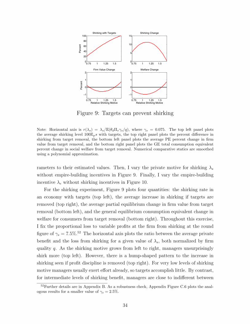
0.75 1 1.25 1.50

20

40

60

80

100Shirking with Targets

Perc

ent

0.75 1 1.25 1.50

5

10

15Shirking Change

0.75 1 1.25 1.5

−1

0

1

2Firm Value Change

Relative Shirking Motive

Perc

ent

0.75 1 1.25 1.5

−1

0

1

2

Relative Shirking Motive

Welfare Change

Student Version of MATLAB

Figure 9: Targets can prevent shirking

Note: Horizontal axis is r(�s) = �s/E(✓d⇧v�s/q), where �s = 0.075. The top left panel plotsthe average shirking level 100Eµs with targets, the top right panel plots the percent di↵erence inshirking from target removal, the bottom left panel plots the average PE percent change in firmvalue from target removal, and the bottom right panel plots the GE total consumption equivalentpercent change in social welfare from target removal. Numerical comparative statics are smoothedusing a polynomial approximation.

rameters to their estimated values. Then, I vary the private motive for shirking �s

without empire-building incentives in Figure 9. Finally, I vary the empire-building

incentive �e without shirking incentives in Figure 10.

For the shirking experiment, Figure 9 plots four quantities: the shirking rate in

an economy with targets (top left), the average increase in shirking if targets are

removed (top right), the average partial equilibrium change in firm value from target

removal (bottom left), and the general equilibrium consumption equivalent change in

welfare for consumers from target removal (bottom right). Throughout this exercise,

I fix the proportional loss to variable profits at the firm from shirking at the round

figure of �s = 7.5%.52 The horizontal axis plots the ratio between the average private

benefit and the loss from shirking for a given value of �s, both normalized by firm

quality q. As the shirking motive grows from left to right, managers unsurprisingly

shirk more (top left). However, there is a hump-shaped pattern to the increase in

shirking seen if profit discipline is removed (top right). For very low levels of shirking

motive managers usually exert e↵ort already, so targets accomplish little. By contrast,

for intermediate levels of shirking benefit, managers are close to indi↵erent between

52Further details are in Appendix B. As a robustness check, Appendix Figure C.6 plots the anal-ogous results for a smaller value of �s = 2.5%.

34

shirking or e↵ort, and targets cause a relatively large portion of managers to provide

e↵ort. Finally, if managers receive large shirking benefits, miss costs do not dissuade

shirking much. The hump-shaped pattern to the prevention of shirking feeds into

counterfactual changes in firm value and social welfare. For intermediate levels of

private shirking benefits, average firm value would be lower if a firm removed targets

even though targets distort R&D (bottom left). The production loss from shirking

if targets are removed also leads to a loss for the aggregate household, so targets

enhance welfare when they prevent a lot of costly shirking (bottom right).

For the empire-building exercise reported in Figure 10, the horizontal axis in each

panel is equal to the ratio between the manager’s private return to size and their aver-

age return to variable profits, both normalized by firm quality q. As empire-building

motives grow from left to right, the R&D-to-sales ratio unsurprisingly increases (top

left). However, the scope for targets to provide discipline, or the change in the R&D-

to-sales ratio when targets are removed, increases as well (top right). For relatively

low empire motives, firms gain in partial equilibrium from target removal (bottom

left). However, for higher empire motives firms would lose value on average from tar-

get removal because of the resulting overinvestment. By contrast, in this experiment

the aggregate household always experiences higher welfare when targets are removed

(bottom right). Firms realize producer surplus, but managers ignore consumer sur-

plus as emphasized by Jones and Williams (2000). The result is underinvestment in

R&D relative to its social value, and targets exacerbate this underinvestment.53

If managers behave badly, Figures 9 and 10 suggest that firm owners may ben-

efit from exploiting outside analyst targets. In principle, discontinuous incentives

might be improved upon even further. Although a full optimal contracting analy-

sis is beyond the scope of the paper, Appendix C reports the additional firm value

from optimally chosen incentives within a class of smooth polynomial contracts. The

resulting improvement is small, with substantially less than 1% in incremental firm

value typically resulting from implementation of smooth incentives relative to tar-

gets. In an environment with information frictions or space constraints in financial

reporting, discontinuous targets may be a particularly logical disciplining device.

Figures 9 and 10 reveal ambiguity in the net welfare impact of short-termist incen-

tives. If shirking is prevalent, consumers may benefit from the discipline of short-term

targets. However, if empire-building matters most, then consumers may lose. By con-

trast with the welfare implications, the growth implications are entirely clear-cut. In

particular, short-termist incentives universally lead to reductions in growth ranging

53Di↵usion of average quality to lagging firms leads to a separate ine�ciency.

35

0.21 0.23 0.25 0.27 0.2914.5

15

15.5

16R&D to Sales with Targets

Perc

ent

0.21 0.23 0.25 0.27 0.290

0.5

1

1.5

2R&D to Sales Change

0.21 0.23 0.25 0.27 0.29−0.2

0

0.2

0.4

Relative Empire Motive

Firm Value Change

Perc

ent

0.21 0.23 0.25 0.27 0.29

−1

0

1

2Welfare Change

Relative Empire Motive

Student Version of MATLAB

Figure 10: Targets can restrain empires

Note: Horizontal axis is r(�e) = �e/E(✓d⇧v/q). The top left panel plots the average R&D to salesratio with targets, the top right panel plots the percent di↵erence in the R&D to sales ratio fromtarget removal, the bottom left panel plots the average PE percent change in firm value from targetremoval, and the bottom right panel plots the GE total consumption equivalent percent change insocial welfare from target removal. Numerical comparative statics are smoothed using a polynomialapproximation.

from 0.04% to 0.09% in this section’s experiments.

7 Conclusion

In the data, profits bunch directly above short-term targets. Firms just meeting

targets have lower R&D growth, and managers just missing receive lower pay. These

patterns suggest both short-termist incentives for managers as well as manipulation

of R&D. An estimated model of macro growth due to micro-level R&D reveals that

short-termist targets matter quantitatively. More volatile R&D at firms leads to a

drop in firm value of around 1% at the micro level and lower growth by around 0.1%

per year at the macro level.

For decades, economists and commentators have expressed concerns with potential

distortions to long-term investment caused by short-termism incentives. The sizable

loss in growth which I quantify provides at least a partial validation of such concerns.

As policymakers seek to promote the benefits from liquid capital markets, transparent

reporting procedures, and increased manager discipline, my results suggest caution.

Closely linked short-termist behavior causes a large drag on long-term growth.

36

ReferencesAcemoglu, Daron, Ufuk Akcigit, Nicholas Bloom, and William R Kerr (2013), “Inno-vation, Reallocation, and Growth.” Working paper.

Acemoglu, Daron and Dan Cao (2015), “Innovation by entrants and incumbents.”Journal of Economic Theory, 157, 255–294.

Aghion, Philippe and Peter Howitt (1992), “A Model of Growth through CreativeDestruction.” Econometrica, 323–351.

Aghion, Philippe, John Van Reenen, and Luigi Zingales (2013), “Innovation andInstitutional Ownership.” American Economic Review, 103, 277–304.

Aguiar, Mark and Gita Gopinath (2007), “Emerging Market Business Cycles: TheCycle is the Trend.” Journal of Political Economy, 115, 69–102.

Allen, Eric J and Patricia M Dechow (2013), “The ‘Rationality’ of the Long DistanceRunner: Prospect Theory and the Marathon.” Working paper.

Altonji, Joseph G and Lewis M Segal (1996), “Small-sample bias in gmm estimationof covariance structures.” Journal of Business & Economic Statistics, 14, 353–366.

Alvarez, Fernando E, Francisco J Buera, and Robert E Lucas Jr (2008), “Models ofIdea Flows.” Working paper.

Asch, Beth J (1990), “Do Incentives Matter? The Case of Navy Recruiters.” Industrialand Labor Relations Review, 89S–106S.

Asker, John, Allan Collard-Wexler, and Jan De Loecker (2013), “Dynamic Inputsand Resource (Mis)Allocation.” Journal of Political Economy.

Asker, John, Joan Farre-Mensa, and Alexander Ljungqvist (2014), “Corporate In-vestment and Stock Market Listing: A Puzzle?” Working paper.

Baber, William R, Patricia M Fairfield, and James A Haggard (1991), “The E↵ect ofConcern about Reported Income on Discretionary Spending Decisions: The Caseof Research and Development.” Accounting Review, 818–829.

Baker, Scott R, Nicholas Bloom, and Stephen J. Terry (2016), “Does UncertaintyReduce Growth? Using Disasters as Natural Experiments.” Working paper.

Barlevy, Gadi (2004), “The Cost of Business Cycles under Endogenous Growth.”American Economic Review, 94, 964–990.

Barlevy, Gadi (2007), “On the cyclicality of research and development.” The Ameri-can Economic Review, 97, 1131–1164.

Barton, Dominic (2011), “Capitalism for the Long Term.” Harvard Business Review.Bartov, Eli, Dan Givoly, and Carla Hayn (2002), “The Rewards to Meeting or BeatingEarnings Expectations.” Journal of Accounting and Economics, 33, 173–204.

Berger, David and Joseph Vavra (2015), “Consumption dynamics during recessions.”Econometrica, 83, 101–154.

Bernstein, Shai (2015), “Does going public a↵ect innovation?” The Journal of Fi-nance, 70, 1365–1403.

Beyer, Anne, Ilan Guttman, and Ivan Marinovic (2014), “Optimal Contracts withPerformance Manipulation.” Journal of Accounting Research, 52, 817–847.

Bhojraj, Sanjeev, Paul Hribar, Marc Picconi, and John McInnis (2009), “MakingSense of Cents: An Examination of Firms that Marginally Miss or Beat AnalystForecasts.” The Journal of Finance, 64, 2361–2388.

Bloom, Nicholas, Paul Romer, Stephen J Terry, and John Van Reenen (2016),“Trapped factors and china’s impact on global growth.” Working paper.

Blundell, Richard, Rachel Gri�th, and Frank Windmeijer (2002), “Individual e↵ectsand dynamics in count data models.” Journal of Econometrics, 108, 113–131.

Borisova, Ginka and James R Brown (2013), “R&D Sensitivity to Asset Sale Proceeds:New Evidence on Financing Constraints and Intangible Investment.” Journal ofBanking & Finance, 37, 159–173.

37

Bradshaw, Mark T and Richard G Sloan (2002), “GAAP versus the Street: An Empir-ical Assessment of Two Alternative Definitions of Earnings.” Journal of AccountingResearch, 40, 41–66.

Brown, James R, Steven M Fazzari, and Bruce C Petersen (2009), “Financing in-novation and growth: Cash flow, external equity, and the 1990s r&d boom.” TheJournal of Finance, 64, 151–185.

Brown, James R and Bruce C Petersen (2009), “Why Has the Investment-Cash FlowSensitivity Declined So Sharply? Rising R&D and Equity Market Developments.”Journal of Banking & Finance, 33, 971–984.

Brown, Lawrence D, Andrew C Call, Michael B Clement, and Nathan Y Sharp (2015),“Inside the black box of sell-side financial analysts.” Journal of Accounting Re-search, 53, 1–47.

Budish, Eric, Benjamin N. Roin, and Heidi Williams (2015), “Do Firms Underin-vest in Long-Term Research? Evidence from Cancer Clinical Trials.” AmericanEconomic Review.

Burgstahler, David and Elizabeth Chuk (2013), “What Have We Learned AboutEarnings Management? Correcting Disinformation about Discontinuities.” Work-ing paper.

Burgstahler, David and Michael Eames (2006), “Management of Earnings and Ana-lysts’ Forecasts to Achieve Zero and Small Positive Earnings Surprises.” Journalof Business Finance & Accounting, 33, 633–652.

Chetty, Raj, John N Friedman, Tore Olsen, and Luigi Pistaferri (2011), “AdjustmentCosts, Firm Responses, and Micro vs. Macro Labor Supply Elasticities: Evidencefrom Danish Tax Records.” Quarterly Journal of Economics, 126, 749–804.

Corrado, Carol, Jonathan Haskel, Cecilia Jona-Lasinio, and Massimiliano Iommi(2013), “Innovation and Intangible Investment in Europe, Japan, and the UnitedStates.” Oxford Review of Economic Policy, 29, 261–286.

Costinot, Arnaud and Andres Rodrıguez-Clare (2015), “Chapter 4. Trade Theorywith Numbers: Quantifying the Consequences of Globalization.” Handbook of In-ternational Economics, 197 – 261.

Daly, Mary, Bart Hobijn, and Brian Lucking (2012), “Why Has Wage Growth StayedStrong?” Federal Reserve Bank of San Francisco Economic Letter.

Davis, Steven J and John Haltiwanger (1992), “Gross Job Creation, Gross Job De-struction, and Employment Reallocation.” Quarterly Journal of Economics, 107,819–863.

Dichev, Ilia, John Graham, Campbell R Harvey, and Shiva Rajgopal (2013), “Earn-ings Quality: Evidence from the Field.” Journal of Accounting and Economics, 56,1–33.

Edmans, Alex, Vivian W Fang, and Katharina A Lewellen (2013), “Equity Vestingand Managerial Myopia.” Working paper.

Edmans, Alex, Xavier Gabaix, and Augustin Landier (2009), “A Multiplicative Modelof Optimal CEO Incentives in Market Equilibrium.” Review of Financial Studies,22, 4881–4917.

Eisfeldt, Andrea L and Camelia M Kuhnen (2013), “CEO Turnover in a CompetitiveAssignment Framework.” Journal of Financial Economics, 109, 351–372.

Eisfeldt, Andrea L and Dimitris Papanikolaou (2013), “Organization Capital and theCross-Section of Expected Returns.” Journal of Finance, 68, 1365–1406.

Eisfeldt, Andrea L and Dimitris Papanikolaou (2014), “The Value and Ownershipof Intangible Capital.” American Economic Review: Papers and Proceedings, 104,1–8.

Fazzari, Steven M, R Glenn Hubbard, Bruce C Petersen, Alan S Blinder, and James MPoterba (1988), “Financing constraints and corporate investment.” Brookings pa-pers on economic activity, 1988, 141–206.

38

Franco, Francesco and Thomas Philippon (2007), “Firms and Aggregate Dynamics.”Review of Economics and Statistics, 89, 587–600.

Garicano, Luis, Claire Lelarge, and John Van Reenen (2013), “Firm Size Distortionsand the Productivity Distribution: Evidence from France.” Working paper.

Gentzkow, Matthew and Jesse M. Shapiro (2014), “Measuring the Sensitivity of Pa-rameter Estimates to Sample Statistics.” Working paper.

Gigler, Frank, Chandra Kanodia, Haresh Sapra, and Raghu Venugopalan (2014),“How frequent financial reporting can cause managerial short-termism: An analysisof the costs and benefits of increasing reporting frequency.” Journal of AccountingResearch, 52, 357–387.

Gilchrist, Simon and Charles P Himmelberg (1995), “Evidence on the role of cashflow for investment.” Journal of monetary Economics, 36, 541–572.

Glover, Brent and Oliver Levine (2014), “Idiosyncratic Risk and the Manager.” Work-ing paper.

Gourio, Francois (2008), “Estimating Firm-Level Risk.” Working paper.Gourio, Francois and Nicolas Roys (2014), “Size-dependent regulations, firm sizedistribution, and reallocation.” Quantitative Economics, 5, 377–416.

Gourio, Francois and Leena Rudanko (2014), “Customer Capital.” Review of Eco-nomic Studies.

Graham, John R, Campbell R Harvey, and Shiva Rajgopal (2005), “The EconomicImplications of Corporate Financial Reporting.” Journal of Accounting and Eco-nomics, 40, 3–73.

Grossman, Gene M and Elhanan Helpman (1991), “Quality Ladders in the Theoryof Growth.” Review of Economic Studies, 58, 43–61.

Grossman, Sanford J and Oliver D Hart (1983), “An Analysis of the Principal-AgentProblem.” Econometrica, 7–45.

Gunny, Katherine A (2010), “The Relation between Earnings Management Using RealActivities Manipulation and Future Performance: Evidence from Meeting EarningsBenchmarks.” Contemporary Accounting Research, 27, 855–888.

Haldane, Andrew G and Richard Davies (2011), “The Short Long.” Bank of EnglandSpeech.

Hall, Robert E (2009), “Reconciling Cyclical Movements in the Marginal Value ofTime and the Marginal Product of Labor.” Journal of Political Economy, 117,281–323.

Hassan, Tarek A and Thomas M Mertens (2011), “The Social Cost of Near-RationalInvestment.” Working paper.

Hennessy, Christopher A and Toni MWhited (2007), “How Costly is External Financ-ing? Evidence from a Structural Estimation.” Journal of Finance, 62, 1705–1745.

Himmelberg, Charles P and Bruce C Petersen (1994), “R & d and internal finance: Apanel study of small firms in high-tech industries.” The Review of Economics andStatistics, 38–51.

Hong, Harrison and Marcin Kacperczyk (2010), “Competition and Bias.” QuarterlyJournal of Economics, 125, 1683–1725.

Hsieh, Chang-Tai and Peter J Klenow (2009), “Misallocation and Manufacturing TFPin China and India.” Quarterly Journal of Economics, 124, 1403–1448.

Iacopetta, Maurizio, Raoul Minetti, and Pietro F. Peretto (2015), “Financial Markets,Industry Dynamics, and Growth.” Working paper.

Imbens, Guido and Karthik Kalyanaraman (2011), “Optimal Bandwidth Choice forthe Regression Discontinuity Estimator.” Review of Economic Studies.

Imbs, Jean (2007), “Growth and Volatility.” Journal of Monetary Economics, 54,1848–1862.

Jensen, Michael C (1986), “Agency Costs of Free Cash Flow, Corporate Finance, andTakeovers.” American Economic Review, 323–329.

39

Jenter, Dirk and Fadi Kanaan (Forthcoming), “CEO Turnover and Relative Perfor-mance Evaluation.” Journal of Finance.

Jenter, Dirk and Katharina Lewellen (2010), “Performance-Induced CEO Turnover.”Working paper.

Jones, Charles I (1995), “Time Series Tests of Endogenous Growth Models.”QuarterlyJournal of Economics, 110, 495–525.

Jones, Charles I and John C Williams (2000), “Too Much of a Good Thing? TheEconomics of Investment in R&D.” Journal of Economic Growth, 5, 65–85.

Kanodia, Chandra and Haresh Sapra (2015), “A Real E↵ects Perspective to Account-ing Measurement and Disclosure: Implications and Insight for Future Research.”Working paper.

Kaplan, Steven N and Luigi Zingales (1997), “Do investment-cash flow sensitivitiesprovide useful measures of financing constraints?” Quarterly Journal of Economics,112, 169–215.

Kasznik, Ron and Maureen F McNichols (2002), “Does Meeting Earnings Expecta-tions Matter? Evidence from Analyst Forecast Revisions and Share Prices.” Journalof Accounting Research, 40, 727–759.

Khan, Aubhik and Julia K Thomas (2008), “Idiosyncratic Shocks and the Role ofNonconvexities in Plant and Aggregate Investment Dynamics.” Econometrica, 76,395–436.

Klette, Tor Jakob and Samuel Kortum (2004), “Innovating firms and aggregate inno-vation.” Journal of Political Economy, 112, 986–1018.

Krusell, Per, Toshihiko Mukoyama, Aysegul Sahin, and Jr. Anthony A. Smith (2009),“Revisiting the Welfare E↵ects of Eliminating Business Cycles.” Review of Eco-nomic Dynamics, 12, 393–402.

Larkin, Ian (2014), “The Cost of High-Powered Incentives: Employee Gaming inEnterprise Software Sales.” Journal of Labor Economics, 32, 199–227.

Levitt, Arthur (1998), “The numbers game.” Remarks by SEC Chairman to the NYUCenter for Law and Business.

Li, Wendy C.Y. (2012), “Depreciation of business r&d capital.” Working paper.Liu, Laura Xiaolei, Toni M Whited, and Lu Zhang (2009), “Investment-Based Ex-pected Stock Returns.” Journal of Political Economy, 117, 1105–1139.

Lucas, Robert E (2003), “Macroeconomic Priorities.” American Economic Review,93, 1–14.

Lucas, Robert E and Benjamin Moll (2011), “Knowledge Growth and the Allocationof Time.” Working paper.

MacKinlay, A Craig (1997), “Event Studies in Economics and Finance.” Journal ofeconomic literature, 35, 13–39.

Mairesse, Jacques, Bronwyn Hall, Lee Branstetter, and Bruno Crepon (1999), DoesCash Flow Ccause Investment and R&D? An Exploration Using Panel Data forFrench, Japanese, and United States Scientific Firms, 129–56. Cambridge Univer-sity Press Cambridge.

Marinovic, Ivan, Marco Ottaviani, and Peter N. Sorensen (2012), “Forecasters’ Ob-jectives and Strategies.” Handbook of Economic Forecasting, 2.

Marko↵, John (1990), “A Corporate Lag in Research Funds is Causing Worry.” NewYork Times, January 23.

Matsunaga, Steven R and Chul W Park (2001), “The E↵ect of Missing a QuarterlyEarnings Benchmark on the CEO’s Annual Bonus.” Accounting Review, 76, 313–332.

Mayer, Colin (2012), “‘Short-Termism’ is a Very British Problem.” Financial Times,July 19.

McCrary, Justin (2008), “Manipulation of the Running Variable in the RegressionDiscontinuity Design: A Density Test.” Journal of Econometrics, 142, 698–714.

40

McGrattan, Ellen R and Edward C Prescott (2014), “A Reassessment of Real BusinessCycle Theory.” American Economic Review: Paper and Proceedings.

McNichols, Maureen (1989), “Evidence of Informational Asymmetries from Manage-ment Earnings Forecasts and Stock Returns.” Accounting Review, 1–27.

Melitz, Marc J and Stephen J Redding (2013), “Firm Heterogeneity and AggregateWelfare.” Working paper.

Michie, Jonathan (2001), Reader’s Guide to the Social Sciences. Fitzroy Dearborn.Moussawi, Rabih (2006), Linking IBES and CRSP Data. Wharton Research DataServices documentation.

Murphy, Kevin J (1999), “Executive Compensation.” Handbook of Labor Economics,3, 2485–2563.

Murphy, Kevin J (2001), “Performance Standards in Incentive Contracts.” Journalof Accounting and Economics, 30, 245–278.

Nikolov, Boris and Toni M Whited (2014), “Agency conflicts and cash: Estimatesfrom a dynamic model.” The Journal of Finance, 69, 1883–1921.

Oyer, Paul (1998), “Fiscal Year Ends and Nonlinear Incentive Contracts: The E↵ecton Business Seasonality.” Quarterly Journal of Economics, 149–185.

Payne, Je↵ L and Wayne B Thomas (2003), “The Implications of Using Stock-SplitAdjusted I/B/E/S Data in Empirical Research.” Accounting Review, 78, 1049–1067.

Perla, Jesse and Christopher Tonetti (2014), “Equilibrium Imitation and Growth.”Journal of Political Economy, 122, 52–76.

Peters, Michael (2013), “Heterogeneous Mark-Ups, Growth and Endogenous Misal-location.” Working paper.

Politis, Dimitris N and Joseph P Romano (1994), “The Stationary Bootstrap.” Jour-nal of the American Statistical Association, 89, 1303–1313.

Rahmandad, Hazhir, Nelson P Repenning, and Rebecca M Henderson (2014), “Mak-ing the Numbers?” Short Termism” & the Puzzle of Only Occasional Disaster.”Working paper.

Ramey, Garey and Valerie Ann Ramey (1995), “Cross-Country Evidence on the Linkbetween Volatility and Growth.” American Economic Review, 85, 1138–51.

Restuccia, Diego and Richard Rogerson (2008), “Policy Distortions and AggregateProductivity with Heterogeneous Establishments.” Review of Economic Dynamics,11, 707–720.

Romer, Paul M (1990), “Endogenous Technological Change.” Journal of PoliticalEconomy, S71–S102.

Roychowdhury, Sugata (2006), “Earnings Management through Real Activities Ma-nipulation.” Journal of Accounting and Economics, 42, 335–370.

Roys, Nicolas (2011), “Persistence of Shocks, Employment and Wages.” Workingpaper.

Sampson, Thomas (2016), “Dynamic selection: An idea flows theory of entry, trade,and growth.” The Quarterly Journal of Economics, 131, 315–380.

Schwenkler, Gustavo, Diogo Duarte, and Kyonghwan Lee (2015), “The Systemic Ef-fects of Benchmarking.” Working paper.

Stein, Jeremy C (1989), “E�cient Capital Markets, Ine�cient Firms: A Model ofMyopic Corporate Behavior.” Quarterly Journal of Economics, 104, 655–669.

Stein, Jeremy C (2003), “Agency, Information and Corporate Investment.” Handbookof the Economics of Finance, 1, 111–165.

Stein, Luke C.D. and Charles C. Y. Wang (2014), “Economic Uncertainty and Earn-ings Management.” Working Paper.

Strebulaev, Ilya A and Toni M Whited (2012), “Dynamic Models and StructuralEstimation in Corporate Finance.” Foundations and Trends in Finance, 6, 1–163.

41

Sun, Bo (2014), “Asset returns under periodic revelations of earnings management.”International Economic Review, 55, 255–282.

Taylor, Lucian A (2010), “Why Are CEOs Rarely Fired? Evidence from StructuralEstimation.” Journal of Finance, 65, 2051–2087.

Yang, Mu-Jeung (2014), “Micro-level Misallocation and Selection: Estimation andAggregate Implications.” Working paper.

Yermack, David and Yuanzhi Li (2014), “Evasive Shareholder Meetings.” Workingpaper.

Young, Eric R (2010), “Solving the Incomplete Markets Model with Aggregate Un-certainty Using the Krusell–Smith Algorithm and Non-Stochastic Simulations.”Journal of Economic Dynamics and Control, 34, 36–41.

Zakolyukina, Anastasia A. (2013), “Measuring Intentional Manipulation: A Struc-tural Approach.” Working paper.

Zbaracki, Mark J, Mark Ritson, Daniel Levy, Shantanu Dutta, and Mark Bergen(2004), “Managerial and Customer Costs of Price Adjustment: Direct Evidencefrom Industrial Markets.” Review of Economics and Statistics, 86, 514–533.

42