The Macro Impact of Short-Termism

Stephen J. Terry⇤

Boston University

July 14, 2015

Abstract

There is a long concern in economics that investor pressure can induce managerialshort-termism, which I examine through the lens of analyst earnings targets. Managersface a tradeo↵ between short-run profits and long-run investment. This paper startsempirically by showing that firms that just meet earnings targets lower their investmentin R&D and intangibles. Firms that just miss their earnings targets cut CEO pay andface drops in stock-market valuation. The paper then builds and structurally estimatesa quantitative general equilibrium endogenous growth model with heterogeneous firms,R&D and accounting manipulation choices, and endogenous earnings forecasts. In themodel, the short-run pressure to meet earnings forecasts cuts growth because R&D ismisallocated across firms, responding too much to short-run profit shocks. This e↵ectcuts growth rates by almost 0.1%, costing the US economy around 6% of output eachcentury. Extending the model to include managerial shirking and empire-building re-veals that earnings targets can improve firm value but may still reduce long-run growthand consumer welfare.

Keywords: Short-Termism, Earnings Manipulation, Heterogeneous Agents, Endoge-nous Growth, Agency Conflicts, Shirking, Empire Building

⇤A previous version of this paper circulated as “The Macro Impact of Firm Earnings Targets.” Please findthe latest version of the paper at www.stanford.edu/

~

sterry/files/MIFET_LATEST_DRAFT.pdf. Email:stephent@bu.edu. Mailing Address: Boston University, Department of Economics, 270 Bay State Road,Boston, MA 02215. I would like to gratefully acknowledge funding for this project as a Bradley DissertationFellow from the Stanford Institute for Economic Policy Research. The paper has benefited from advicefrom Nick Bloom, Pete Klenow, Bob Hall, Monika Piazzesi, Nir Jaimovich, Ed Knotek, Itay Saporta-Eksten,Brent Bundick, Julia Thomas, Aubhik Khan, Jon Willis, Jordan Rappaport, Chris Tonetti, Mike Dinerstein,John Mondragon, Nicola Bianchi, Ivan Marinovic, and numerous seminar participants.

1

1 Introduction

For over a century economists have been concerned that pressure from investors for short-

term results can damage the long-run growth of companies. For example, Alfred Marshall

famously wrote in 1890 that people act like “children who pick the plums out of their pudding

to eat them at once.” This paper examines the macroeconomic growth implications of short-

termism through the lens of analyst earnings targets, a particularly prevalent and observable

manifestation of short-term pressure today.1

The benefits from investments in research and development (R&D) or other intangible

expenditures may either fail to materialize or appear only much later. Yet the costs of these

long-term investments generally must be borne today. In a particularly important example

of this tradeo↵, R&D must be immediately subtracted or expensed from profits according to

the Generally Accepted Accounting Principles (GAAP) governing public firms in the US.2

If failure to deliver short-term results has adverse consequences, firms or managers may

therefore be willing to sacrifice some long-term value to deliver higher profit now. Economic

theory for decades has modeled overall growth and changes in aggregate productivity as

the result of long-term investment at the microeconomic level. So a heavy dependence of

long-term investment on short-term pressures can be crucial for understanding the process of

economic growth in the macroeconomy.3 Furthermore, factors impacting long-term growth

disproportionately a↵ect the economy in quantitative terms because of their compounding

e↵ects. This paper takes several concrete steps towards empirically documenting and struc-

turally quantifying the costs of short-termism, through the lens of pressure to meet earnings

forecasts, on innovative investments, long-term growth, and welfare.

Research analysts at stock brokerages routinely forecast the earnings of public companies.

Firms publicly release statements of earnings, an accounting measure of profitability also

known as net income or simply profits, at the end of each fiscal quarter and year. The

1See Marshall (1890) for the quote, as well as Haldane and Davies (2011), Mayer (2012), Marko↵ (1990),or Michie (2001) for additional perspectives on short-termism. See also Budish et al. (Forthcoming) for arecent empirical treatment of apparent short-termist distortions of long-term investment in cancer drugs.

2See Financial Accounting Standards Board (FASB) rule 730-10-25-1 for the explicit statement of therule in 2014 US GAAP. By contrast, EU accounting guidelines do allow for discretionary depreciation oramortization of R&D development costs (PricewaterhouseCoopers, 2013).

3See, for example, work by Romer (1990), Aghion and Howitt (1992), Grossman and Helpman (1991), orAcemoglu et al. (2013). Also, note that a recent strand of papers models endogenous growth as the productof idea flows (Perla and Tonetti, 2014; Lucas and Moll, 2011; Alvarez et al., 2008; Sampson, 2014). Sinceexploiting idea flows remains costly for firms, the tradeo↵ between growth and performance remains.

2

financial press as well as equity market participants follow these releases closely during

earnings season. Around 90% of the respondents to a broad survey of managers in Dichev

et al. (2013) report systematic pressure, internal and external to their firms, to meet earnings

benchmarks. Consistent with these reports, Figure I displays the annual distribution of the

di↵erence between realized and forecast earnings (forecast errors), scaled by firm assets for

a panel of US public firms. A disproportionate number of firm-years report zero or just

positive earnings forecast errors, i.e. display profits that just meet or beat analyst forecasts,

while the mass of forecast errors is hollowed out just below zero.4

Earnings benchmarks and potential concerns about short-termism are not exclusive to

public firms. Interestingly, surveys of private and public firm managers reveal quite similar

rates of reported earnings pressure.5 However, the pressures and incentives surrounding in-

novation at large public firms, measured directly in this paper, are independently interesting

for our broad understanding of innovation in the macroeconomy. Public firms undertake

almost two-thirds (67%) of all non-government R&D expenditures in the United States.6

A long history of research into apparent real earnings manipulation by public firms also

suggests that R&D investments systematically and discontinuously change around earnings

benchmarks or targets including analyst forecasts of profits.7 More broadly, a literature on

investments in technology notes that budgeting deadlines and agency frictions within firms

can constrain the ability of organizations to invest in improved productivity, and other work

in economic history suggests that the presence of sharp performance targets may contribute

to overall ine�ciency.8

My paper first establishes two empirical facts using a merged database of analyst forecasts

4Marinovic et al. (2012) and Hong and Kacperczyk (2010) overview analyst earnings forecasts.Burgstahler and Chuk (2013) emphasizes that the discontinuity in Figure I is robust. The McCrary (2008)sorting test strongly rejects continuity of the distribution at the zero forecast error level. See Garicano et al.(2013), Gourio and Roys (2012), Chetty et al. (2011), Daly et al. (2012), and Allen and Dechow (2013), re-spectively for evidence of similar bunching in French firm sizes around regulatory thresholds, Danish incomearound tax kinks, nominal wage changes around zero, and even marathon finish times around focal points.

5See Dichev et al. (2013), Table 13.6The R&D statistic reflects the aggregation of R&D expenditures in my baseline sample from Compustat

(xrd) compared to aggregate research expenditures in 2000 from the NSF Survey of Industrial Research andDevelopment (total private R&D). Note that recent empirical studies by Bernstein (2012), Aghion et al.(2013), or Asker et al. (2014) suggest that the quality and quantity of innovation and investment at publiclytraded firms can either be lower than in their private counterparts or hinge crucially upon factors such asinstitutional ownership with long horizons.

7See for example, Bhojraj et al. (2009), Baber et al. (1991), Roychowdhury (2006), or Gunny (2010).8See Liebman and Mahoney (2013) for a study in the US government and Atkin et al. (2014) for an

experiment Pakistani manufacturing. See Meng et al. (Forthcoming) for evidence that food procurementquotas across regions may have contributed to the severity of the Great Famine in China.

3

and firm accounting data. First, firms that just meet or beat analyst forecasts in a particular

year exhibit discontinuously lower R&D and broader intangibles investment growth. There

is a drop of around 30% in mean R&D and intangibles growth relative to firms that just

fail to meet earnings forecasts. Such discontinuities, detected using flexible nonparametric

regression discontinuity estimators, are consistent with systematic manipulation of long-term

investment to meet analyst forecasts of earnings. Relatedly, a survey of executives at large

US public firms in Graham et al. (2005) corroborates the result: almost half of managers

reveal that they would reject a positive net present value project if taking the project meant

missing analyst forecasts of earnings.9 In a second empirical contribution, the paper then

applies the same techniques to inspect manager incentives and stock returns. CEOs just

failing to deliver profits above consensus analyst expectations face drops of around 7% in

total compensation. Earnings pressure is not limited to solely the CEO of a company. The

several most highly paid executives in a company face around 5% less total compensation for

just failing to meet analyst targets. Furthermore, stock returns are discontinuously lower for

firms just failing to meet earnings targets. Firms that just fail to meet earnings targets see

around 0.64% lower abnormal cumulative returns in a ten-day window to the earnings release

date. The finding of apparent compensation incentives for managers to deliver short-term

results, together with capital market pressures, helps to motivate real earnings manipulation

but also concurs with a large literature on performance-based incentives and the relationship

between earnings announcements and returns.10

Building o↵ of my empirical findings, the second part of the paper builds a theoretical

model linking earnings targets and aggregate growth. The model features managers of het-

erogeneous firms making R&D investment decisions together with pure paper or accounting

manipulation choices subject to both persistent and transitory profitability shocks. R&D

expenditures by firms result in random innovation arrival according to a quality ladder struc-

ture that aggregates in general equilibrium. Earnings forecasts, endogenously produced by

an outside sector of analysts, provide short-term pressure on managers who seek to avoid

costs resulting from failure to meet earnings forecasts. The model is agnostic about the

9Firms of course can use paper or accounting rather than operational or real decisions to boost earningsabove analyst forecasts. Studies such as Burgstahler and Eames (2006) document that discretionary accrualsappear to be unusually high for firms just meeting earnings targets.

10See, for example, Larkin (2014), Oyer (1998), Murphy (1999), Murphy (2001), Matsunaga and Park(2001), Edmans et al. (2013), Jenter and Lewellen (2010), Jenter and Kanaan (Forthcoming), Eisfeldt andKuhnen (2013), and Asch (1990), Bhojraj et al. (2009), Bartov et al. (2002).

4

source of these costs for managers, but in practice earnings miss costs may be purely private

to the manager due to reputational or career concerns (Dichev et al., 2013), borne by the

firm due to higher external finance costs or disrupted communication costs with outsiders

(Graham et al., 2005), or even the result of explicit manager compensation policies chosen

by firms (Matsunaga and Park, 2001).11

After laying out the model structure, the paper employs numerical solution methods and

parametrizes the model using a combination of calibration and structural GMM estimation.

Structural estimation here exploits the moments of R&D expenditures, sales, and forecast

errors in a panel of firm-level data on thousands of large US public firms to produce a

“Baseline” quantitative model economy. My main quantitative results in the paper compare

the Baseline environment with a “No Targets” counterfactual economy in which there are

no costs or incentives for managers to meet or beat earnings forecasts.

The Baseline model with earnings targets for firms qualitatively reproduces the kinked

earnings forecast error distribution in Figure I, with a disproportionate mass of firm-years

just above targets and a hollowing out the forecast error distribution below zero. The

counterfactual No Targets economy, by contrast, fails to reproduce a kinked distribution.

Furthermore, while the No Targets economy produces a smooth distribution of R&D growth

across the zero forecast error threshold, the Baseline model leads to a cut in R&D growth

for firms just meeting earnings targets, consistent with the empirical evidence from the first

portion of the paper. Finally, the counterfactual exercise reveals insights into a body of

research in corporate finance studying the release of information contained within earnings

releases and surprises (Stein, 1989; MacKinlay, 1997). Firms in the Baseline model with

mediocre profitability shocks are able to find the resources, either in long-term investment

manipulation or paper obfuscation, to boost earnings above target. Therefore, firms that

miss an earnings forecast in equilibrium are far less profitable than firms meeting or beating

earnings forecasts, a quantitative di↵erence which is positive but muted by contrast in the

No Targets economy. Such considerations may help to explain why firms report increased

pressure from outsiders to explain or divulge more information about the prospects of the

firm if they miss analyst expectations. The information revelation upon missing an earnings

target also naturally helps to motivate the change in stock returns I document empirically

for firms just failing to meet earnings targets.

11In my model-based calculations, I choose between these alternatives in a manner which results in con-servative estimates of the costs of earnings targets.

5

Within the model, short-termism can be defined as responsiveness of forward-looking

R&D policies to purely transitory or short-term shocks to profitability, even when those

shocks contain no information about the profitability of innovation in the long term. The

Baseline economy features such short-termism, resulting in lower and more volatile R&D

expenditures.12 Increased volatility impacts the overall e�ciency of R&D expenditures for

firms even absent any e↵ects on levels, since my theoretical structure includes curvature

or diminishing returns to R&D. Just as Barlevy (2004) theoretically links business cycle

volatility to reduced growth in the macroeconomy in the presence of diminishing returns

to investments, my model implies that firms subject to transitory profitability shocks and

choosing more volatile R&D expenditures have fewer innovation arrivals than would result

from a smoother long-term investment path.13 At the microeconomic level the result is

lower firm value on average, an approximately 1% reduction in mean firm value in the

Baseline economy relative to the No Targets case. By studying the distortion to long-

term investments resulting from earnings targets, I contribute to a literature on structural

estimation in dynamic corporate finance which outlines the costs to firms resulting from, for

example, financial frictions, CEO firing costs, or agency frictions surrounding cash holding

and investment.14

At the macroeconomic level, the Baseline economy with earnings targets is characterized

by lower aggregate growth of around 2.25% per year relative to a growth rate of around

2.31% per year in the No Targets environment. By exhibiting short-termism and responding

to purely transitory profitability shocks with their long-term R&D investments, manager

earnings pressure causes a sort of research misallocation, whereby the e�ciency of aggregate

innovation declines.15 Small changes in permanent growth rates translate into quantitatively

large di↵erences in welfare, because these changes are continuously compounded over time.

In my model, the removal of earnings targets results in an overall increase in welfare of

0.44%, i.e. consumption in each period would need to be increased by almost half a percent

in the Baseline to make the aggregate household as well o↵ as in the No Targets balanced

12High R&D sensitivity to profitability echoes empirical work in corporate finance. See, for example,Borisova and Brown (2013), Brown and Petersen (2009), and Mairesse et al. (1999).

13For further macroeconomic work on the link between volatility and growth, see for example Ramey andRamey (1995) or Imbs (2007).

14See Hennessy and Whited (2007), Taylor (2010), and Nikolov and Whited (2010), respectively. Strebu-laev and Whited (2012) provides an overview of structural estimation in dynamic corporate finance.

15The misallocation from profitability volatility is distinct from but related to the broader literature onmisallocation in Hsieh and Klenow (2009), Restuccia and Rogerson (2008), Peters (2013), Asker et al. (2013),or Yang (2014).

6

growth path.16 For comparison, recent quantitative estimates of the welfare gains from the

elimination of business cycles are around 0.1-1.8%, or the static gains from trade according to

recent work could be approximately 2.0-2.5%.17 Overall, short-termism from earnings targets

results in a quantitatively large distortion to long-term growth and the macroeconomy.

The main quantitative contribution of the paper should be interpreted as the delineation

of the costs of earnings targets as outlined above. However, earnings targets may of course

also provide benefits to firms or society, omitted from the baseline cost measurements.18 For

example, earnings forecasts may contribute to more accurate valuation of firms or alleviate

financial frictions at otherwise healthy firms. In fact, a series of recent theoretical and

empirical papers indicates that alleviation of financial frictions or the liberalization of equity

markets can indeed reap e�ciency gains from better allocation of resources throughout the

macroeconomy.19 A second source of potential benefits from earnings targets operates within

firms through the provision of discipline to managers in the presence of agency conflicts.

Compensation schemes which explicitly or implicitly punish managers for failure to meet

publicly observable earnings forecasts may lead to firm or social gains. The final portion of

the paper analyzes multiple sources of agency conflicts within the existing model of dynamic

manager investment used initially to estimate the costs of earnings pressure.

A corporate finance investment literature emphasizes that firms are riddled with agency

frictions leading to a wedge between the interests of managers and firms as a whole (Stein,

2003). Two classic forms of agency conflict include unobservable shirking by managers (Ed-

mans et al., 2009; Grossman and Hart, 1983) and empire building motivated by private

manager benefits from size or investment (Nikolov and Whited, 2010; Jensen, 1986). When

managers can provide low e↵ort, I show that for strong enough shirking motives earnings

targets within manager compensation contracts may improve value for firms as well as social

welfare. The dynamic distortion to long-term investment, while costly, may be overwhelmed

16US consumption was around $11,500 billion in 2013 according to the BEA as of March 2014, so a 0.44%increase in consumption is equivalent to a permanent increase in consumption of around $51 billion eachyear. The overall welfare gains decompose into 1.32% dynamic gains from growth rate changes and a staticloss of -0.86% due to higher initial investment in R&D.

17See Krusell et al. (2009) for the welfare consequences of business cycles, Costinot and Rodrıguez-Clare(2015) or Melitz and Redding (2013) for the welfare gains from trade. Also, see Hassan and Mertens (2011)for the social cost of “near-rationality” in investment, around 2.4% in consumption-equivalent terms.

18An interpretation of this sort is the norm for cost calculations in macroeconomics, with the most promi-nent example being the literature on the costs of business cycles (Lucas, 2003; Barlevy, 2004; Krusell et al.,2009). Gains from the elimination of business cycles may not be achievable if their elimination is costly.

19See, for example, Midrigan and Xu (2014), Moll (Forthcoming),Buera and Shin (2013), Buera et al.(2011), or Campello et al. (2014).

7

by the gains to levels obtained from increased discipline. In a second case, when firm agency

conflicts are instead characterized by empire-building tendencies for managers, earnings tar-

gets may improve firm value by restraining R&D investments. If the social and private

returns to R&D di↵er, however, restraint of R&D through earnings pressure can lead to an

exacerbation of underinvestment from the social perspective and an increase in social losses

from earnings targets.

So, the model’s implications depend crucially on assumptions about the exact form of

agency conflicts within firms. Motivated by this consideration, I focus on qualitative results

within my discussion of the benefits of earnings targets, demonstrating possibilities over a

broad range of model parametrizations.

Section 2 of the paper describes my data and lays out the empirical results linking earnings

forecasts, long-term investment, and CEO incentives. Section 3 describes the quantitative

model of earnings pressure and growth, together with my numerical solution and estimation

strategy. Section 4 performs the main quantitative analysis estimating the costs of short-

termism for firms and the macroeconomy. Section 5 explores potential agency benefits from

short-term pressure. Section 6 concludes. Appendixes follow describing the data (Appendix

A), theory (Appendix B), and numerical solution method (Appendix C).

2 Data and Empirical Discontinuities

This section empirically investigates the manipulation of long-term investment and incentives

for executives surrounding earnings targets for firms. First, after joining analyst forecasts of

earnings with the accounting releases of US public firms, my analysis reveals that firms just

meeting earnings targets exhibit substantially lower long-term investment growth in R&D

as well as broader intangibles. Similarly, CEOs and other executives at firms just failing to

meet earnings targets receive discontinuously lower compensation.

This paper draws on data from two main sources. First, I use millions of earnings

forecasts at the firm-analyst level from the Institutional Brokers Estimates System (I/B/E/S)

database. Actual or realized values of firm “Street” earnings per share accompany the analyst

forecasts in I/B/E/S.20 I also use Compustat data drawn from the annual accounting reports

of public firms.

20So-called Street earnings, over which firms possess moderate discretion, are the appropriate measure ofearnings for my purposes, since Street earnings are more widely followed by financial market participantsand observers than the net income measures reported in Compustat (Bradshaw and Sloan, 2002).

8

Linking the I/B/E/S and Compustat datasets results in a panel of around 25,000 firm-

fiscal year observations with consensus analyst forecasts, Street realizations, and basic ac-

counting outcomes. Around 4,000 firms from 1983-2010 are available in the combined un-

balanced panel. The sample primarily consists of larger firms, accounting for around 11%

of US employment, 67% of all US private R&D expenditures, and total sales of around 31%

of US GDP.21 See Data Appendix Table A.I for descriptive statistics on the sample. I also

incorporate Execucomp data on CEO and executive compensation where possible, as well

as Center for Research in Security Prices (CRSP) data on stock returns. Data Appendix

A provides further information on the datasets, the sample restrictions imposed, and the

construction of individual variables.

If managers face incentives to meet earnings forecasts, then firms should avoid reporting

profits just below analyst forecasts if possible, instead taking actions throughout their fiscal

year to satisfy expectations. In this section I employ a flexible empirical tool, nonparametric

regression discontinuity techniques, to identify exactly this type of earnings manipulation

through changes in the distribution of long-term investment as firms just meet forecasts. By

the first application of regression discontinuity estimators to my knowledge in this context,

I contribute to a literature which treats similar results as prima facie evidence of earnings

manipulation by firms.22

Throughout the empirical analysis, my preferred measure of the forecast error for a

particular firm j in year t is the realized value of Street earnings Streetjt

minus the median

analyst forecast of firm earnings made from the middle of the same fiscal year Street

f

jt

scaled by firm assets. This measure of earnings forecast errors is a standard one used in

accounting studies (Burgstahler and Eames, 2006; Burgstahler and Chuk, 2013).

Forecast errors serve as the running variable in my regression discontinuity estimation

with a cutpoint of zero. The first measure of investment I consider at firms is the tangible

investment rate. Since tangible capital expenditures are depreciated from earnings over time

rather than immediately expensed as incurred, their impact on current earnings and hence

usefulness as a tool for earnings manipulation is diluted. Ex-ante, therefore, I expect little

21For these comparisons, US employment is total nonfarm payrolls according to the BLS in 2000 (St.Louis FRED variable PAYEMS), while Compustat employment is the variable emp. US R&D expendituresare drawn from the National Science Foundation Survey of Industrial Research and Development in 2000,with R&D for the corresponding year from Compustat variable xrd. US nominal GDP in 2000 comes fromthe BEA (St. Louis FRED variable GDPA), with Compustat gross sales in variable sale.

22See, for example, Roychowdhury (2006), Gunny (2010), Baber et al. (1991), or Burgstahler and Eames(2006).

9

change in tangible investment rates for firms just meeting earnings targets. By contrast,

two measures of long-term investment, R&D expenditures and broader “Intangibles” expen-

ditures are both immediately expensed from earnings in the period incurred.23 A growing

empirical literature within economics and finance concludes that long-term investment ex-

penditures contribute to long-term profitability for firms, to aggregate productivity over the

business cycle, and to an improved explanation of stock returns in the cross section of firms.24

The first three columns of Table I above report regression discontinuity estimates of the

predicted di↵erence in the tangible investment rate, overall intangible expenditures growth,

and R&D growth for firms just meeting their earnings targets in a given year relative to

firms failing to meet an earnings target. I compute results using outcomes demeaned by

firm then year, controlling for both permanent trend heterogeneity across firms in long-term

investments as well as business cycle e↵ects.25 I detect no discontinuity in tangible investment

rates. By contrast, R&D growth and overall intangibles growth are both approximately

2.5% lower for firms just meeting an earnings target. The discontinuities are statistically

significant and economically meaningful, each representing a cut of around 30% of average

annual long-term investment growth.26

Note that I make no direct causal claims from my regression discontinuity results of the

form that is typically relied upon in applied microeconomics (Lee and Lemieux, 2010). By

contrast, the apparent endogenous “sorting” of firms to the right of the zero forecast error

cutpoint, which would typically be considered a threat to identification, lies at the very

core of my argument for the economic impacts of earnings targets. In a later section, I

build and estimate a quantitative model of R&D investment and earnings forecasts. The

model demonstrates that reduced R&D growth around the zero forecast error threshold

23Intangibles expenditures are equal to selling, general, and administrative (SG&A) expenditures. SG&A,a basic accounting item, enjoys extensive coverage within the Compustat database and include not onlyR&D expenses but also a range of other nonproduction expenses such as management labor compensation,training expenditures, and advertising costs.

24See for example Eisfeldt and Papanikolaou (2013, 2014), Gourio and Rudanko (2014), McGrattan andPrescott (2014), Hall (2004), Corrado et al. (2009), Corrado et al. (2013), or Corrado et al. (2012).

25Of course this implies that the results from Table I are based upon a two-stage procedure. Table I followsthe literature by relying upon straightforward clustering at the firm level in the calculation of standard errors.For robustness, however, Table A.III in Data Appendix A reports the results with no qualitative changes froma block bootstrap procedure taking into account within-firm correlation as well as uncertainty associatedwith the first-stage demeaning of outcome variables.

26For all the regression discontinuity tests in this section, see Table A.II in Data Appendix A for placebochecks. Data Appendix Figure A.I plots a range of robustness checks with bandwidth choice alternatives tothe optimal Imbens and Kalyanaraman (2011) value used in Table I. Placebo checks reveal no significantbreaks at alternative cutpoints away from 0, and bandwidth plots reveal robustness.

10

should be expected in the presence of incentives for managers to meet earnings targets but

would otherwise be absent. Such results structurally support the convenient use of regression

discontinuity methodology as a detection mechanism in this context.

Pressure to meet earnings targets can represent the product of explicit e↵orts of the dis-

tributed shareholders or boards of firms to provide discipline to CEOs and managers with

interests divergent from their own. Therefore, discipline for managers may be evident in ob-

served compensation for the CEO or for the several most highly paid executives in a firm.27

Table I displays estimated discontinuities in pay. CEOs that generate earnings just below an-

alyst forecasts earn approximately 7% less, while the top managers as a whole receive around

5% lower compensation. Discontinuous manager incentives in my sample link to a litera-

ture in corporate finance and accounting that documents either discontinuities in manager

compensation at earnings benchmarks or interaction between investment responses to earn-

ings targets and CEO equity incentives (Matsunaga and Park, 2001; Edmans et al., 2013).

However, just as in the case of long-term investments, my results represent to my knowledge

the first application of regression discontinuity methodology to the study of earnings target

incentives.

Finally, Table I also documents a discontinuity in abnormal returns. Firms just failing

to meet targets have approximately 0.64% lower cumulative abnormal returns in a ten-day

window to the earnings release date. This result corroborates literature on the information

content within earnings releases as well as on a capital market premium to meeting or

beating analyst expectations.28 However, also note that horizon matters for the interaction

between earnings targets and outcomes. Changes in long-term investments such as R&D

expenditures over the course of the year naturally take time to implement. The results in

this paper therefore reflect earnings forecasts made for the full fiscal year from the perspective

of the middle of the year, i.e. from a two-quarter horizon. The single exception to this rule

is the discontinuity in abnormal returns, which I document using a forecast horizon of one

quarter. Following the related discussion of forecast horizons in Bhojraj et al. (2009), I

feel that these timing choices strike the appropriate balance between allowing for R&D and

investment choices to be implemented, on the one hand, and incorporating a fuller range of

information available to capital market participants when examining return patterns on the

other hand.

27In this paper, total compensation includes salary, bonuses, and the value of stock option-based pay.28See, for example, the results contained in Stein (1989), MacKinlay (1997), and Bartov et al. (2002).

11

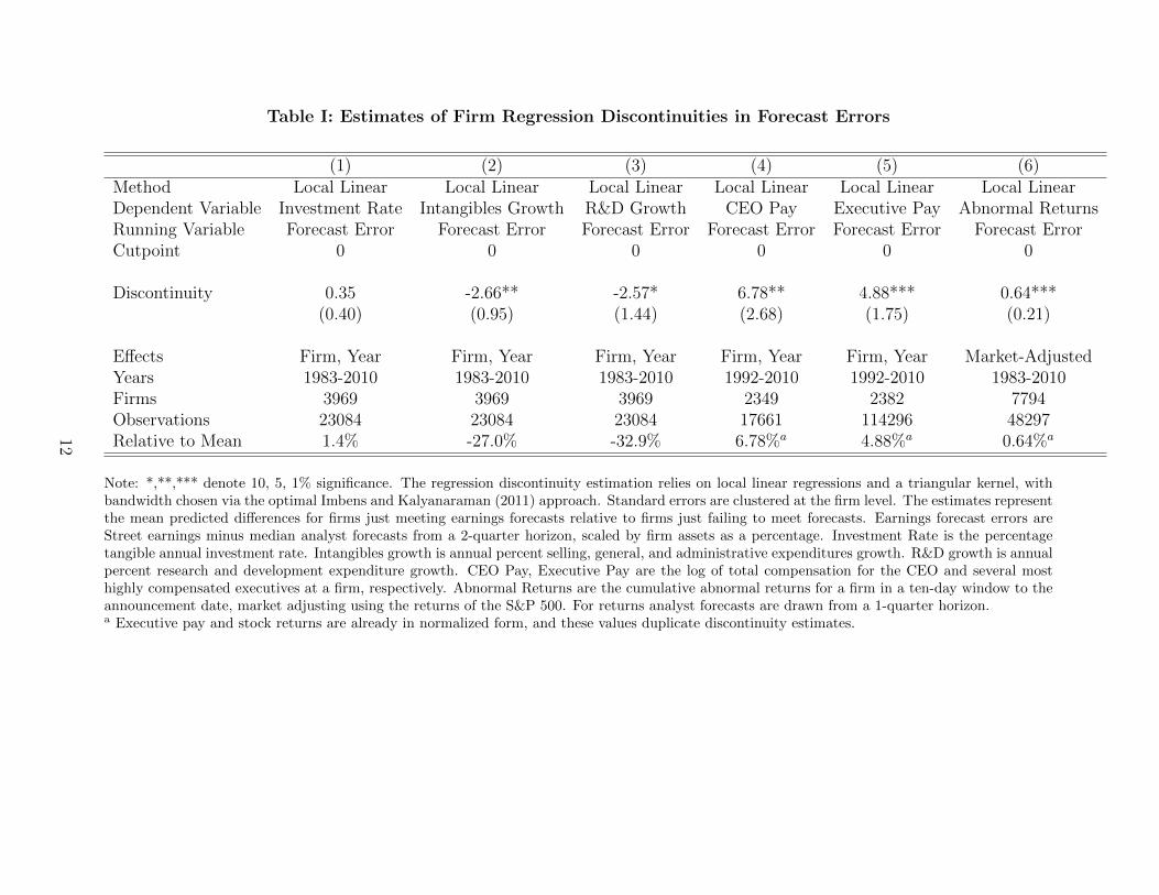
Table I: Estimates of Firm Regression Discontinuities in Forecast Errors

(1) (2) (3) (4) (5) (6)Method Local Linear Local Linear Local Linear Local Linear Local Linear Local LinearDependent Variable Investment Rate Intangibles Growth R&D Growth CEO Pay Executive Pay Abnormal ReturnsRunning Variable Forecast Error Forecast Error Forecast Error Forecast Error Forecast Error Forecast ErrorCutpoint 0 0 0 0 0 0

Discontinuity 0.35 -2.66** -2.57* 6.78** 4.88*** 0.64***(0.40) (0.95) (1.44) (2.68) (1.75) (0.21)

E↵ects Firm, Year Firm, Year Firm, Year Firm, Year Firm, Year Market-AdjustedYears 1983-2010 1983-2010 1983-2010 1992-2010 1992-2010 1983-2010Firms 3969 3969 3969 2349 2382 7794Observations 23084 23084 23084 17661 114296 48297Relative to Mean 1.4% -27.0% -32.9% 6.78%a 4.88%a 0.64%a

Note: *,**,*** denote 10, 5, 1% significance. The regression discontinuity estimation relies on local linear regressions and a triangular kernel, withbandwidth chosen via the optimal Imbens and Kalyanaraman (2011) approach. Standard errors are clustered at the firm level. The estimates representthe mean predicted di↵erences for firms just meeting earnings forecasts relative to firms just failing to meet forecasts. Earnings forecast errors areStreet earnings minus median analyst forecasts from a 2-quarter horizon, scaled by firm assets as a percentage. Investment Rate is the percentagetangible annual investment rate. Intangibles growth is annual percent selling, general, and administrative expenditures growth. R&D growth is annualpercent research and development expenditure growth. CEO Pay, Executive Pay are the log of total compensation for the CEO and several mosthighly compensated executives at a firm, respectively. Abnormal Returns are the cumulative abnormal returns for a firm in a ten-day window to theannouncement date, market adjusting using the returns of the S&P 500. For returns analyst forecasts are drawn from a 1-quarter horizon.a Executive pay and stock returns are already in normalized form, and these values duplicate discontinuity estimates.

12

3 Model of Earnings Pressure and Growth

In this section I build a quantitative model of endogenous growth and earnings targets,

followed by a discussion of the equilibrium concept and numerical solution method. Finally,

I explain my parametrization of the model based on GMM structural estimation using firm-

level moments from my Compustat and I/B/E/S sample.

3.1 Baseline Model Structure

Time is discrete, and a representative household subject to no aggregate uncertainty maxi-

mizes utility from a flow of aggregate consumption Ct denominated in units of a final good.

Period utility takes a standard constant relative risk aversion form with subjective discount

rate ⇢ and intertemporal elasticity of substitution 1

�. The household purchases shares Sjt at

price Pjt, receives dividendsDjt from a fixed continuum of intermediate goods firms j 2 [0, 1],

and inelastically supplies a fixed amount of labor L to a final goods sector at wage rate wt.

The household problem is

maxCt,Bt+1,{Sjt}

1X

t=0

⇢

t C1��t

1� �

Ct +Bt+1

+

Z

1

0

PjtSjtdj = RtBt + wtL+

Z

1

0

(Pjt +Djt)Sjt�1

dj.

The household also makes a savings choice Bt+1

in a one-period bond with interest rate Rt+1

.

As is standard, in general equilibrium household Euler equations will link growth rates and

firm policies to this interest rate. Furthermore, on the balanced growth path which I will

consider in this paper, interest rates will be fixed at a value R. The numeraire final good is

produced by a competitive, constant returns to scale, and price-taking sector which combines

intermediate goods Xjt from each firm j, and demands labor in the amount LDt to produce

output Yt in each period. The labor share is �, and the final goods technology is

Yt =L

Dt�

(1� �)

Z

1

0

[Qjt(ajt + "jt)]�X

1��jt dj.

As will be discussed in more detail below, each intermediate goods firm at time t possesses

both a quality level Qjt, together with an exogenous profitability shock ajt+ "jt.29 Together,

these quantities determine the marginal product of intermediate input Xjt in final goods

29The intermediate goods firm profitability shock is the sum of persistent ajt

and transitory "jt

.

13

production. The final goods problem is

max{Xjt},LD

t

Yt �Z

1

0

pjtXjtdj � wtLDt .

The form of the final goods sector optimization problem above, which follows Acemoglu and

Cao (Forthcoming), yields a standard isoelastic downward-sloping demand curve for variety

j, given by

Xjt = p

�1/�jt LQjt(ajt + "jt).

Each member of the fixed continuum of intermediate goods firms j 2 [0, 1] faces idiosyn-

cratic uncertainty.30 Firm j is associated with a manager who in each period determines its

monopoly price pjt, R&D investment zjt, and paper or accounting manipulation mjt. Firm

j’s long-term quality level Qjt is nonstationary and grows from R&D investments according

to a quality ladder structure. Simultaneously, stationary exogenous profitability shocks ajt

and "jt satisfy

ajt = (1� ⇢a) + ⇢aajt�1

+ ⇣jt, ⇣jt ⇠ N(0, �2

a)

"jt ⇠ N(0, �2

").

The transitory shock process "jt bu↵ets firm profitability in each period, while the AR(1)

process ajt persists. A number of recent papers apply a similar basic structure, decomposing

volatility a↵ecting firm or economy-wide investment choices into persistent and transitory

components, and of course transitory-persistent shock breakdowns have a long history in

labor economics.31 Variable profits ⇧v(Qjt, ajt, "jt, pjt) in firm j equal total revenue minus

total production costs. Intermediate goods firms can convert final goods output to variety j

of intermediate output at constant marginal cost , yielding

⇧v(Qjt, ajt, "jt, pjt) = pjtXjt � Xjt.

The isoelastic form of the final goods sector’s demand for input j implies an optimal constant

markup pricing rule for pjt over marginal cost ,32 so that eventually variable profits take

30Throughout the paper, I abstract from entry and exit with a fixed set of intermediate goods firms. Thisassumption is made more palatable by my structural estimation of the model with data from large publicfirms with lower exit hazards. However, I abstract from the Schumpeterian interactions between entry andinnovation studied in endogenous growth models starting with Aghion and Howitt (1992).

31Such papers for firm investments include Aguiar and Gopinath (2007), Franco and Philippon (2007),Roys (2011), and Gourio (2008), while Blundell et al. (2008) and many others consider household persistentand transitory shock decompositions in the presence of a consumption/savings choice.

32For notational convenience, following Acemoglu and Cao (Forthcoming), I make the assumption that = 1� �, leading to a monopoly price of p

jt

= 1��

1��

= 1.

14

the following homogenous form in Qjt:

⇧v(Qjt, ajt, "jt, pjt) = �Qjt(ajt + "jt)L.

Firm j’s scaled R&D choice zjt leads to a total expenditure of zjtQjt and results in an

innovation with probability �(zjt) = Az

↵jt. The parameter ↵ 2 (0, 1) governs the elasticity

of innovation arrival with respect to R&D. Innovations embody a proportional improvement

up a quality ladder by amount � > 1, so that the level of long-term quality Qjt+1

for firm j

in period t+ 1 is

Qjt+1

=

⇢

�Qjt, with probability �(zjt)max(Qjt,!Qt+1

), with probability 1� �(zjt).

Eventually, if firm j lags and does not innovate for long enough, the firm will receive a

di↵usion of some small fraction ! of the average quality level Qt+1

of the economy as a

whole.33

Managers also make discretionary accounting choices which a↵ect reported earnings.

Empirically, paper manipulation by public firms can be accomplished through judicious use

of tools such as heavy revenue accrual or recognition into earnings within a fiscal period.

Through their accounting discretion, managers may also shift their reported Street earnings

from a value which would be determined by strict application of GAAP principles to the

more flexible value reported in the financial press. However, activities such as accruals

manipulation bear costs for at least two reasons. First, by recognizing revenues now firms

constrain their ability to count those revenues towards earnings in future. Second, more

discretionary accounting manipulation involves more disruption of manager time, higher

auditor expenses, or even higher probability of fraud detection and prosecution.34 In the

model, by choosing manipulation level mjt firm j can induce a net paper shift of its reported

earnings bymjtQjt subject to a quadratic cost �mm2

jtQjt. Overall earnings ⇧Streetjt reported in

the model are defined as variable profits net of R&D expenditures and paper manipulation:

⇧Streetjt = ⇧v(Qjt, ajt, "jt, pjt)� zjtQjt +mjtQjt.

33The di↵usion structure follows Acemoglu and Cao (Forthcoming) and is useful to deliver existence of astationary distribution of normalized firm-level quality levels Q

jt

on a balanced growth path for the economy.34See Dichev et al. (2013) for a survey-based discussion of the costs of earnings manipulation perceived

by managers at large firms in the United States. See Bradshaw and Sloan (2002) for a further discussionof the distinction between Street and GAAP earnings in practice. See Zakolyukina (2013) for a structuralmodel of paper accounting manipulation. See Druz et al. (2015) for a discussion of manipulation of earningsconference calls through manager tone.

15

For individual firms, forecasts of earnings evolve over time based on the rational projec-

tions of an outside sector of identical equity analysts. Since earnings ⇧Streetjt are homogeneous

in long-term quality Qjt, analysts forecast normalized earnings ⇡jt ⌘ ⇧Streetjt /Qjt. Analysts

understand the structure of the economy, including the exogenous shock processes and the

potential for earnings manipulation by firms. Forecasters possess an information set at time

t consisting of lagged normalized earnings ⇡jt�1

, consistent with survey evidence in Brown

et al. (2014) revealing that large fractions of equity analysts incorporate recent earnings per-

formance into the production of their earnings forecasts.35 Further motivated by empirical

evidence suggesting that analysts face career concerns and pressure to produce accurate fore-

casts of earnings,36 in the model forecasts ⇡fjt(⇡jt�1

) minimize the following ex-ante expected

quadratic loss function:

⇡

fjt = argmin

⇡fE⇡jt�1(⇡

f � ⇡jt)2

.

Optimally forecasts in the model therefore satisfy ⇡

fjt(⇡jt�1

) = E(⇡jt|⇡jt�1

), and firm j is

aware of its earnings forecast ⇡fjt when making R&D investment and paper manipulation

choices in period t.

The manager of firm j maximizes the expected discounted flow of their personal utility.37

Their decisions solve

max{zjt,mjt,pjt}t

E( 1X

t=0

✓

1

R

◆t

D

Mjt

)

.

Manager compensation depends on a constant, exogenous share ✓d of ownership in their

firm. Given manager choices for R&D, accounting manipulation, and pricing, firm dividends

in period t equal variable profits minus R&D expenditures and resource costs of paper

manipulation:

Djt = ⇧v(Qjt, ajt, "jt, pjt)� zjtQjt � �

2

mmjtQjt.

35In practice, analysts may of course use more information for forecasts than lagged earnings alone. How-ever, Numerical Appendix Table C.III demonstrates that within the model a lagged earnings informationset results in high forecast accuracy. In particular, only marginal improvements in forecasting performancewould result from broader information sets including lagged forecast errors or R&D expenditures.

36See, for example, Hong et al. (2000), Hong and Kubik (2003), or Hong and Kacperczyk (2010). Theoret-ical frameworks using analyst objective function based on squared-error loss include Marinovic et al. (2012)and Beyer and Guttman (2011).

37Managers discount their flow utility using the interest rate R implied by household decisions. In TheoryAppendix B, I provide details of a microfoundation of this discounting structure with overlapping generationsof one period-lived managers selling a manager franchise onwards to the next period’s manager after choosingfirm policies.

16

Manager flow utility, linear in consumption and other payo↵s, is given by

D

Mjt = ✓dDjt � ⇠I(⇧Street

jt < ⇧fjt)Qjt.

The first term in D

Mjt simply represents the manager’s dividend share. The second term

contains the impact of firm earnings forecasts on the manager objective and hence firm

policies. A manager who fails to deliver earnings which meet or beat analyst expectations

su↵ers a fixed loss governed by the parameter ⇠ � 0. In particular, however, when ⇠ = 0 the

manager problem results in firm profit maximization. Although in Section 5 I will explicitly

examine the potential for other agency frictions such as a manager taste for shirking or

empire-building, note that these channels are shut down in my initial framework.

The discontinuous, fixed nature of the miss cost is a natural choice given the kinked

forecast error distribution in Figure 1 as well as the evidence for discontinuous manager

incentives from Section 2. In principle, earnings miss costs can represent three separate

sources of loss for managers

⇠ = ⇠

manager + ✓d⇠firm + (1� ✓d)⇠

pay.

The first potential component of miss costs for managers, ⇠manager, is purely private and

could include career or reputational concerns for managers. Surveyed managers report that

such reputational concerns loom large (Dichev et al., 2013). Alternatively, managers may

su↵er increased e↵ort costs due to higher rates of more negatively focused communications

with outsiders upon an earnings miss (Yermack and Li, 2014).38

The second potential component of miss costs, ⇠firm, reflects any resource, disruption,

or other costs borne by firms rather than directly by managers for failure to meet analyst

expectations. Such firm-borne costs still a↵ect managers through their ownership shares ✓d.

Surveyed managers report that e↵orts to avoiding earnings misses are important to maintain

a low cost of external finance, to avoid triggering debt covenants, and even to avoid higher

likelihood of lawsuits from shareholders (Graham et al., 2005).

The third and final component of miss costs, ⇠pay, represents the potential for a firm

to explicitly condition manager compensation on meeting earnings targets. In particular,

if exogenous compensation includes not only a dividend share but also an amount ⇠payQjt

38Given the focus of my paper on long-term growth rather than fluctuations, I abstract through a constantvalue of ⇠ from potential fluctuations in managerial incentives to meet or beat earnings benchmarks overtime. However, recent empirical evidence presented by Stein and Wang (2014) suggests that such incentivesmay vary with the overall level of economic volatility or uncertainty.

17

clawed back conditional upon a miss, then the net loss to a manager from this channel is

given by (1 � ✓d)⇠pay. Empirically, managers failing to meet earnings benchmarks su↵er

reduced bonuses (Matsunaga and Park, 2001), and the empirical evidence from Section 2

suggests that total compensation is discontinuously lower for managers just failing to meet

analyst forecasts.

My structural estimation approach for quantifying a manager’s cost of missing an earnings

target, will identify only the combined cost ⇠ rather than the three individual components

⇠

manager, ⇠firm, and ⇠

pay. When making quantitative statements about the overall cost

of earnings targets in Section 4, I conservatively assume that the entirety of the term ⇠

represents personal costs ⇠manager. Any changes in firm value or household welfare due to

distorted manager policies are therefore due to the policies themselves rather than a direct

mechanical contribution from resource costs ⇠firm.

3.2 Balanced Growth Path Equilibrium and Numerical Solution

The model outlined above admits a balanced growth path equilibrium at which all model ag-

gregates, including average quality Qt =R

1

0

Qjtdj, grow at constant rate g. Theory Appendix

B outlines the full equilibrium definition, which involves four major optimizing components:

1) optimal household consumption and savings decisions Ct, Sjt, and Bt+1

given the budget

constraint, 2) competitive final goods firm optimization over intermediate goods Xjt and la-

bor demand L

Dt , 3) intermediate goods firm manager optimization over monopoly pricing pjt,

R&D investment zjt, and paper earnings manipulation mjt, and 4) rational analyst forecasts

of earnings ⇡fjt for each firm. An economy-wide resource constraint, labor market clearing,

asset market clearing, and aggregation consistency conditions complete the characterization

of general equilibrium for the model.

I use numerical techniques to solve the model. Given homogeneity of manager returns

in long-term quality, I first normalize their dynamic problem by the average quality level in

the economy Qt. This normalization yields a stationary recursive formulation reported in

Theory Appendix B as a function of four state variables: q (normalized endogenous long-

term quality), a (exogenous persistent profitability), " (exogenous transitory profitability),

and ⇡f (endogenous analyst forecasts of earnings). I notationally omit dependence on j or t

for clarity, indicating future and lagged values by 0 and �1

, respectively. I solve the manager

problem using standard numerical dynamic programming techniques (Judd, 1998). I also

18

rely upon a polynomial approximation to the analyst expectation ⇡

f = E(⇡|⇡�1

).39 For a

given parametrization of the model and solution to the manager’s problem, I compute a

stationary distribution µ(q, a, ", ⇡f ) of firm states.

Model aggregates are a function of the stationary distribution µ. My algorithm for

full general equilibrium solution of the model along a balanced growth path, explained in

more detail in Numerical Appendix C, involves a hybrid dampened fixed-point and bisection

algorithm iterating over the growth rate g, interest rate R, and forecast function ⇡

f (⇡�1

)

such that the following three fixed points are satisfied:

1. The constant interest rate R and growth rate g satisfy the household Euler equation:

R =1

⇢

(1 + g)�

2. An economy-wide growth rate equal to g results from the aggregation of intermediate

goods firm R&D investment policies z and the innovation arrival function �(z):

1 + g =Q

0

Q

=

R

�(z)�qdµ(a, ", q, ⇡f )+R

q>!(1+g)(1� �(z))qdµ(a, ", q, ⇡f )

+R

q!(1+g)(1� �(z))!(1 + g)dµ(a, ", q, ⇡f )

3. Analyst expectations of earnings are consistent with the equilibrium distribution µ:

⇡

f = Eµ(⇡|⇡�1

)

3.3 Estimation with Firm-Level Data

Numerical analysis of the baseline model laid out above requires fixing the values of many

parameters. For the most part I follow a structural estimation strategy based on GMM

using firm-level moments from my joint sample of Compustat and I/B/E/S data. However,

before estimating the model I externally calibrate some of the parameters involving common

quantities from the macroeconomics or innovation literature. Table II reports the values of

these parameters.

The model period is one year. Together, an intertemporal elasticity of substitution of

0.5 or � = 2, a subjective discount rate of ⇢ = 1/1.02 ⇡ 0.98, and a targeted growth rate

39Table C.III in the Numerical Appendix C records forecast accuracy or robustness statistics to alternativeforecast systems with higher order approximations in ⇡�1 above the baseline implementation (a linear rule),as well as to di↵erent information sets including forecast errors and R&D expenditures. In all cases, thehigher-order approximations and extended information sets yield little quantitative gain in forecast accuracy.

19

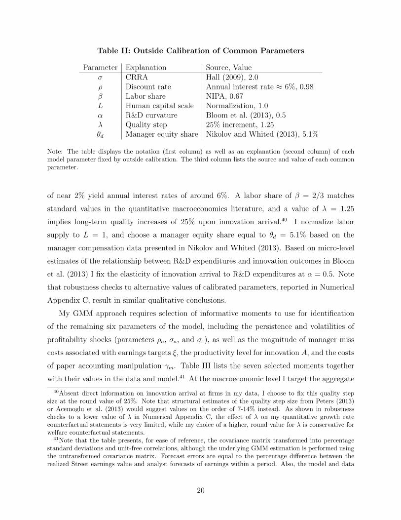
Table II: Outside Calibration of Common Parameters

Parameter Explanation Source, Value� CRRA Hall (2009), 2.0⇢ Discount rate Annual interest rate ⇡ 6%, 0.98� Labor share NIPA, 0.67L Human capital scale Normalization, 1.0↵ R&D curvature Bloom et al. (2013), 0.5� Quality step 25% increment, 1.25✓d Manager equity share Nikolov and Whited (2013), 5.1%

Note: The table displays the notation (first column) as well as an explanation (second column) of eachmodel parameter fixed by outside calibration. The third column lists the source and value of each commonparameter.

of near 2% yield annual interest rates of around 6%. A labor share of � = 2/3 matches

standard values in the quantitative macroeconomics literature, and a value of � = 1.25

implies long-term quality increases of 25% upon innovation arrival.40 I normalize labor

supply to L = 1, and choose a manager equity share equal to ✓d = 5.1% based on the

manager compensation data presented in Nikolov and Whited (2013). Based on micro-level

estimates of the relationship between R&D expenditures and innovation outcomes in Bloom

et al. (2013) I fix the elasticity of innovation arrival to R&D expenditures at ↵ = 0.5. Note

that robustness checks to alternative values of calibrated parameters, reported in Numerical

Appendix C, result in similar qualitative conclusions.

My GMM approach requires selection of informative moments to use for identification

of the remaining six parameters of the model, including the persistence and volatilities of

profitability shocks (parameters ⇢a, �a, and �"), as well as the magnitude of manager miss

costs associated with earnings targets ⇠, the productivity level for innovation A, and the costs

of paper accounting manipulation �m. Table III lists the seven selected moments together

with their values in the data and model.41 At the macroeconomic level I target the aggregate

40Absent direct information on innovation arrival at firms in my data, I choose to fix this quality stepsize at the round value of 25%. Note that structural estimates of the quality step size from Peters (2013)or Acemoglu et al. (2013) would suggest values on the order of 7-14% instead. As shown in robustnesschecks to a lower value of � in Numerical Appendix C, the e↵ect of � on my quantitative growth ratecounterfactual statements is very limited, while my choice of a higher, round value for � is conservative forwelfare counterfactual statements.

41Note that the table presents, for ease of reference, the covariance matrix transformed into percentagestandard deviations and unit-free correlations, although the underlying GMM estimation is performed usingthe untransformed covariance matrix. Forecast errors are equal to the percentage di↵erence between therealized Street earnings value and analyst forecasts of earnings within a period. Also, the model and data

20

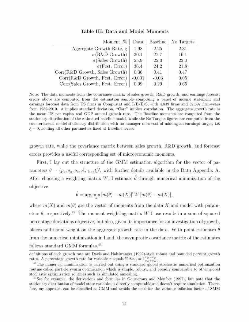
Table III: Data and Model Moments

Moment, % Data Baseline No Targets

Aggregate Growth Rate, g 1.98 2.25 2.31�(R&D Growth) 30.1 27.7 16.1�(Sales Growth) 25.9 22.0 22.0�(Fcst. Error) 36.4 24.2 21.8

Corr(R&D Growth, Sales Growth) 0.36 0.41 0.47Corr(R&D Growth, Fcst. Error) -0.001 -0.03 0.05Corr(Sales Growth, Fcst. Error) 0.09 0.29 0.65

Note: The data moments from the covariance matrix of sales growth, R&D growth, and earnings forecasterrors above are computed from the estimation sample composing a panel of income statement andearnings forecast data from US firms in Compustat and I/B/E/S, with 4,839 firms and 32,597 firm-yearsfrom 1982-2010. � implies standard deviation, “Corr” implies correlation. The aggregate growth rate isthe mean US per capita real GDP annual growth rate. The Baseline moments are computed from thestationary distribution of the estimated baseline model, while the No Targets figures are computed from thecounterfactual model stationary distribution with no manager miss cost of missing an earnings target, i.e.⇠ = 0, holding all other parameters fixed at Baseline levels.

growth rate, while the covariance matrix between sales growth, R&D growth, and forecast

errors provides a useful corresponding set of microeconomic moments.

First, I lay out the structure of the GMM estimation algorithm for the vector of pa-

rameters ✓ = (⇢a, �a, �", A, �m, ⇠)0, with further details available in the Data Appendix A.

After choosing a weighting matrix W , I estimate ✓ through numerical minimization of the

objective

✓ = argmin✓

[m(✓)�m(X)]0 W [m(✓)�m(X)] ,

where m(X) and m(✓) are the vector of moments from the data X and model with param-

eters ✓, respectively.42 The moment weighting matrix W I use results in a sum of squared

percentage deviations objective, but also, given its importance for an investigation of growth,

places additional weight on the aggregate growth rate in the data. With point estimates ✓

from the numerical minimization in hand, the asymptotic covariance matrix of the estimates

follows standard GMM formulas.43

definitions of each growth rate are Davis and Haltiwanger (1992)-style robust and bounded percent growthrates. A percentage growth rate for variable x equals %�x

jt

= 2xjt�xjt�1

xjt+xjt�1.

42The numerical minimization is carried out using a standard global stochastic numerical optimizationroutine called particle swarm optimization which is simple, robust, and broadly comparable to other globalstochastic optimization routines such as simulated annealing.

43See for example, the derivations and formulas in Gourieroux and Monfort (1997), but note that thestationary distribution of model state variables is directly computable and doesn’t require simulation. There-fore, my approach can be classified as GMM and avoids the need for the variance inflation factor of SMM

21

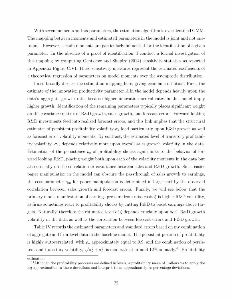
With seven moments and six parameters, the estimation algorithm is overidentified GMM.

The mapping between moments and estimated parameters in the model is joint and not one-

to-one. However, certain moments are particularly influential for the identification of a given

parameter. In the absence of a proof of identification, I conduct a formal investigation of

this mapping by computing Gentzkow and Shapiro (2014) sensitivity statistics as reported

in Appendix Figure C.VI. These sensitivity measures represent the estimated coe�cients of

a theoretical regression of parameters on model moments over the asymptotic distribution.

I also broadly discuss the estimation mapping here, giving economic intuition. First, the

estimate of the innovation productivity parameter A in the model depends heavily upon the

data’s aggregate growth rate, because higher innovation arrival rates in the model imply

higher growth. Identification of the remaining parameters typically places significant weight

on the covariance matrix of R&D growth, sales growth, and forecast errors. Forward-looking

R&D investments feed into realized forecast errors, and this link implies that the structural

estimates of persistent profitability volatility �a load particularly upon R&D growth as well

as forecast error volatility moments. By contrast, the estimated level of transitory profitabil-

ity volatility, �", depends relatively more upon overall sales growth volatility in the data.

Estimation of the persistence ⇢a of profitability shocks again links to the behavior of for-

ward looking R&D, placing weight both upon each of the volatility moments in the data but

also crucially on the correlation or covariance between sales and R&D growth. Since easier

paper manipulation in the model can obscure the passthrough of sales growth to earnings,

the cost parameter �m for paper manipulation is determined in large part by the observed

correlation between sales growth and forecast errors. Finally, we will see below that the

primary model manifestation of earnings pressure from miss costs ⇠ is higher R&D volatility,

as firms sometimes react to profitability shocks by cutting R&D to boost earnings above tar-

gets. Naturally, therefore the estimated level of ⇠ depends crucially upon both R&D growth

volatility in the data as well as the correlation between forecast errors and R&D growth.

Table IV records the estimated parameters and standard errors based on my combination

of aggregate and firm-level data in the baseline model. The persistent portion of profitability

is highly autocorrelated, with ⇢a approximately equal to 0.9, and the combination of persis-

tent and transitory volatility,p

�

2

a + �

2

" , is moderate at around 12% annually.44 Profitability

estimation.44Although the profitability processes are defined in levels, a profitability mean of 1 allows us to apply the

log approximation to these deviations and interpret them approximately as percentage deviations.

22

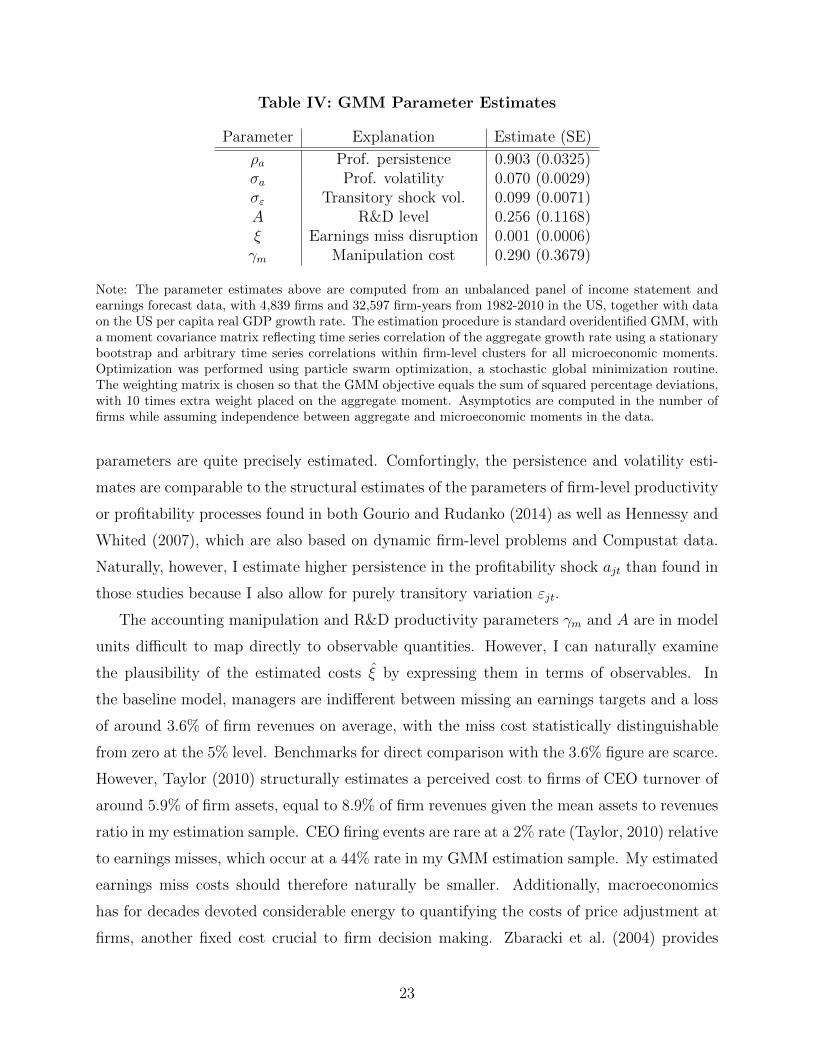
Table IV: GMM Parameter Estimates

Parameter Explanation Estimate (SE)

⇢a Prof. persistence 0.903 (0.0325)�a Prof. volatility 0.070 (0.0029)�" Transitory shock vol. 0.099 (0.0071)A R&D level 0.256 (0.1168)⇠ Earnings miss disruption 0.001 (0.0006)�m Manipulation cost 0.290 (0.3679)

Note: The parameter estimates above are computed from an unbalanced panel of income statement andearnings forecast data, with 4,839 firms and 32,597 firm-years from 1982-2010 in the US, together with dataon the US per capita real GDP growth rate. The estimation procedure is standard overidentified GMM, witha moment covariance matrix reflecting time series correlation of the aggregate growth rate using a stationarybootstrap and arbitrary time series correlations within firm-level clusters for all microeconomic moments.Optimization was performed using particle swarm optimization, a stochastic global minimization routine.The weighting matrix is chosen so that the GMM objective equals the sum of squared percentage deviations,with 10 times extra weight placed on the aggregate moment. Asymptotics are computed in the number offirms while assuming independence between aggregate and microeconomic moments in the data.

parameters are quite precisely estimated. Comfortingly, the persistence and volatility esti-

mates are comparable to the structural estimates of the parameters of firm-level productivity

or profitability processes found in both Gourio and Rudanko (2014) as well as Hennessy and

Whited (2007), which are also based on dynamic firm-level problems and Compustat data.

Naturally, however, I estimate higher persistence in the profitability shock ajt than found in

those studies because I also allow for purely transitory variation "jt.

The accounting manipulation and R&D productivity parameters �m and A are in model

units di�cult to map directly to observable quantities. However, I can naturally examine

the plausibility of the estimated costs ⇠ by expressing them in terms of observables. In

the baseline model, managers are indi↵erent between missing an earnings targets and a loss

of around 3.6% of firm revenues on average, with the miss cost statistically distinguishable

from zero at the 5% level. Benchmarks for direct comparison with the 3.6% figure are scarce.

However, Taylor (2010) structurally estimates a perceived cost to firms of CEO turnover of

around 5.9% of firm assets, equal to 8.9% of firm revenues given the mean assets to revenues

ratio in my estimation sample. CEO firing events are rare at a 2% rate (Taylor, 2010) relative

to earnings misses, which occur at a 44% rate in my GMM estimation sample. My estimated

earnings miss costs should therefore naturally be smaller. Additionally, macroeconomics

has for decades devoted considerable energy to quantifying the costs of price adjustment at

firms, another fixed cost crucial to firm decision making. Zbaracki et al. (2004) provides

23

estimates of the costs at a large firm associated with a price change and dominated by costs

of customer negotiation and communication. These total expenses sum to about 1.2% of

firm revenues in each annual price-changing cycle. Given that price changes predictably

occur each year within firms, a lower direct estimate of price change costs relative to my

structurally estimated costs perceived by managers from earnings misses is reassuring.

Given the overidentified and highly nonlinear structure of the model, I can not in general

expect an exact match between model and data moments. However, Table III demonstrates

that the Baseline model with incentives to meet earnings forecasts leads to a broadly suc-

cessful fit to the data moments.45 In particular, the Baseline delivers an aggregate growth

rate around the 2% level seen in the data, together with substantial variation in sales growth

rates as in the data. Note that the Baseline model delivers somewhat less volatile forecast er-

rors than observed in the data, but higher volatility than a model without earnings pressure

(moments also reported in Table III). Furthermore, in both the Baseline and the data, fore-

cast errors negatively covary very slightly with R&D growth. In other words, the presence

of earnings targets implies that cuts to R&D growth can be driven in the model by a desire

to meet or beat earnings forecasts and therefore be correlated with higher forecast errors.

By contrast, the model without earnings targets, in which R&D innovations are exclusively

motivated by persistent profitability innovations, naturally produces a positive correlation

of forecast errors with R&D growth. Furthermore, the presence of earnings targets in the

Baseline causes dependence of R&D policies on transitory shocks to profitability, increasing

the volatility of R&D growth substantially, while a model without a motive to meet earnings

forecasts underpredicts the R&D volatility seen in the data by a large margin. Finally, the

paper obfuscation in a model with earnings targets leads to lower correlation between sales

growth and forecast errors, closer in line with the data, while a model without earnings

targets overpredicts this correlation by a large amount.

4 Estimated Costs of Short-Termism

With estimated model parameters in hand, I now evaluate the impact of earnings targets

by comparing my Baseline economy with a counterfactual No Targets economy in which

there are no manager costs of missing an earnings forecast. First, I decompose the contrast-

45Note, however, that the amount of data used for GMM estimation of the model implies that the J-testof overidentifying restrictions for the model is quite stringent, producing a strong rejection of the model.

24

ing implications of the Baseline economy and the No Targets model for earnings forecast

errors, R&D growth, and profitability. The presence of pressure to meet earnings targets

endogenously delivers a kinked forecast error distribution, lower R&D growth for firms just

meeting earnings targets, as well as a stark separation of profitability between firms meeting

and missing forecasts. Each of these outcomes is absent or muted in the counterfactual No

Targets economy. Second, I then move to a discussion of the economic costs of earnings tar-

gets. Earnings benchmarks force a distortion to the dynamic long-term investment decisions

of firms in the Baseline model. Because of this e↵ect, I find that the Baseline economy ex-

hibits quantitatively meaningful decreases in aggregate growth rates and household welfare,

lower and more volatile firm R&D expenditures, and lower firm value on average.

4.1 Earnings Manipulation in the Baseline Model

Within my model, Figure II displays the unconditional distribution of earnings forecasts er-

rors in the Baseline (in red bars) and the counterfactual No Targets (in black bars) economies.

Crucially, the model with earnings targets delivers bunching of the forecast error distribution

at zero, as managers engage in both real and paper earnings manipulation to reach earnings

forecasts, as well as a hollowing out of the distribution of earnings forecast errors below

zero.46 Both patterns are generally consistent with the empirical kink in forecasts errors

evident from Figure I. By contrast, the model without earnings targets displays a smoothly

varying distribution of forecast errors.

Figure III displays the conditional mean of percentage R&D growth for firms in the

Baseline (in red) and No Targets economy (in black), given di↵erent values for forecast errors

⇡�⇡

f . While R&D growth varies rather smoothly across the zero forecast error benchmark

in the No Targets economy, firms which are incentivized to meet earnings forecasts in the

Baseline model have R&D growth rates around 1% lower than firms that fail to meet an

earnings target. Clearly a finding of reduced R&D growth by firms just meeting earnings

targets fits naturally into a world with high-pressure earnings forecasts but is not consistent

with a No Targets economy.

A strand of literature within both corporate finance and accounting seeks to understand

46The horizontal axis, based on normalization by long-term firm quality Q

jt

rather than a notion of firmassets, is not directly comparable to the earnings forecast error distribution displayed in Figure I. However,the long-term value and scale of a firm in the model depends heavily upon quality, in a similar fashion tothe heavy dependence of scale upon assets in the estimation sample.

25

the determinants of and information content within earnings releases.47 In a theoretical con-

tribution, Stein (1989) suggests that myopic distortions of investment by firms endogenously

arise in order to boost short-term earnings of profitability in a signal-jamming equilibrium.

An imperfectly informed market expects manipulation and therefore updates its inferences

about firms with poor earnings reports particularly harshly. Anecdotally, this intuition is

consistent the survey of large US firm managers in Graham et al. (2005), where one par-

ticipant reported that “if you see one cockroach, you immediately assume that there are

hundreds behind the walls, even though you may have no proof that this is the case.”

In the context of my model, Figure IV shows quantitative evidence of exactly this type of

selection into meeting earnings targets, with firms that meet forecasts in the Baseline model

146% more profitable on average (as measured by the persistent shock ajt) than firms that

miss a target. By contrast, firms in the No Targets economy that miss an earnings target are

only 11% less profitable on average than firms that meet their targets. Clearly, in the Baseline

model, observers of firms would be justified in inferring quite poor profitability prospects

for firms failing to meet an earnings forecast. I view the results in Figure IV as potentially

suggestive as to the means by which disruptions to firms or managers from earnings misses

could arise. Imperfectly informed analysts, the financial media, or the distributed owners

of public firms may react particularly negatively to an earnings miss and demand manager

time, attention, or even litigation as they seek to gain more information about the underlying

profitability prospects of the firm in question.

The results in Figures II-IV above incorporate measurement error for earnings targets

within the model for the purposes of plotting model outcomes against model forecast er-

rors. Why is this useful? Quantitative models with fixed costs and heterogeneity routinely

yield a stark sorting of agents across a threshold or into adjustment vs. inaction (Khan

and Thomas, 2008; Berger and Vavra, 2014), and my model is no exception. In fact bunch-

ing is strong, and a range of forecast errors just below zero never occur in equilibrium if

measurement error is ignored. The literature routinely incorporates some some quantitative

addition, such as measurement error or maintenance investment depending on the context,

in order to allow for a looser sorting of model stationary distributions. Motivated by these

concerns, Theory Appendix B lays out my extended model of manager decisions with a

decomposition of transitory profitability shocks into two separate components: "jt (known

47See, for example, work by MacKinlay (1997), McNichols (1989), Kasznik and McNichols (2002), or Liuet al. (2009).

26

to managers when policies are decided) and another component ⌫jt (unknown to managers

when policies are decided). In practice ⌫jt serves as “target measurement error,” since the

exact earnings threshold for meeting forecasts is ex-ante uncertain. However, throughout the

rest of the paper in which direct comparison of firm outcomes to forecast errors is not the

object of interest, I conservatively discuss results generated by the Baseline model without

measurement error, since the impact of earnings pressure on growth and welfare turns out

to be slightly lower in this case.48

4.2 Costs of Earnings Targets

Earnings pressure systematically changes real or economic outcomes for firms and the econ-

omy as a whole. Figure V displays the mean of R&D policy z for the Baseline and No Targets

economies conditional upon the value of the transitory shock ". Without earnings pressure,

forward-looking R&D investment in the No Targets economy optimally ignores transitory

profitability shocks and is flat as a function of ". However, by contrast, the Baseline R&D

policy z responds to short-term profitability, declining when profits are low in the current

period.49 Responsiveness of R&D to transitory variation is the primary manifestation of

short-termism in my model. Even though a negative transitory profitability shock does not

contain information about the payo↵ to R&D in future, managers on average cut their long-

term investment to avoid the disruption associated with missing their earnings forecast in the

near term. Overall, earnings targets reduce R&D expenditures z by -0.32% and increase the

standard deviation or volatility of R&D expenditures by 23.1%. The sensitivity of R&D to

transitory profitability shock represents a type of misallocation of R&D, because long-term

investment here deviates from a purely forward-looking optimal policy within the model.

Such sensitivity is also consistent with empirical work in Brown and Petersen (2009); Brown

et al. (2009) finding a high sensitivity of R&D to cash flows in US public firms.50

More R&D volatility resulting from sensitivity to short-term shocks damages the overall

e�ciency of the innovation process. Table V reports the aggregate growth rate in the Baseline

48The interested reader may find analogues to Figures II-IV above, without earnings target measurementerror, in Numerical Appendix Figures C.III-C.V. Also, note that for the purposes of generating Figures II-IV,I calibrate the decomposition of known and unknown transitory shock volatilities to attribute approximatelyhalf of the total estimated transitory volatility to each source.

49In both the Baseline and No Targets economies, of course, higher values of the persistent shock a inducehigher levels of R&D expenditures z on average.

50See also Schmitz (2014) for a related model of business cycles and R&D in which di↵erences in firm sizeinteract with R&D sensitivity to shocks to generate persistent business cycles.

27

Table V: Earnings Targets Reduce Growth, Welfare

% %

g

ˆ⇠ 2.25 � Welfare 0.44g

⇠=0 2.31 � Firm Value 1.03100-yr �Y 5.82

Note: The entries above represent the percent di↵erence in the indicated aggregate quantity between thecounterfactual ⇠ = 0 and estimated benchmark ⇠ cases. The moments are computed from the stationarydistributions µ of the respective economies, and comparisons are across balanced growth paths without atransition path calculation. � Welfare represents the percentage consumption equivalent variation of ⇠ = 0relative to the baseline economy. The change in firm value is the mean partial equilibrium percent changein firm value when ⇠ = ⇠ ! ⇠ = 0 for an individual firm, averaged over the stationary distribution of ⇠.The 100-yr change in Y is the percentage di↵erence in output after 100 years from a no targets growth raterather than a targets growth rate, using identical initial conditions.

model, gˆ⇠ = 2.25%, which is around 6 basis points lower than growth in the No Targets

economy, g⇠=0 = 2.31%. These di↵erences are quantitatively larger than they may at first

appear, since growth changes lead to compounded di↵erences across economies far into the

future. The driving force behind diminished growth in my economy with earnings targets

is curvature in the model link �(z) between R&D expenditures and innovation. Given

concavity or diminishing returns to R&D in �(z), randomly more volatile R&D causes fewer

innovation arrivals on average, even ignoring level changes in R&D expenditures.51

A negative relationship between volatility and growth, crucial to the quantitative results

here, is familiar from the macroeconomics literature. For example, Barlevy (2004) describes

the manner in which at the aggregate level, higher volatility of tangible investment caused by

business cycles can increase the theoretical cost of business cycles by reducing the aggregate

growth rate. The same mechanism appears at the microeconomic level in my Baseline model.

Since macroeconomists routinely infer much higher volatility or variation in profitability at

the disaggregated level than on aggregate (Bloom et al., 2012), my firm-level link between

profit shocks and R&D naturally provides a potent source of changes in the innovative

e�ciency of the economy as a whole.

To gain a better sense of the quantitative magnitude of the distortion to aggregate growth

rates, I also engage in an accounting exercise for aggregate welfare. The second column

of Table V displays the consumption equivalent welfare gain to the aggregate household

from the removal of earnings targets, �W . This welfare gain is the percentage increase

51This statement is a straightforward implication of Jensen’s inequality together with the concavity of theinnovation arrival function �(z) = Az

↵, where ↵ 2 (0, 1).

28

in consumption in each period (around 0.44%) which would make the Baseline household

indi↵erent to the No Targets consumption stream, comparing directly across balanced growth

paths.52 Explicit welfare formulas and a set of quantitative robustness checks are reported

in Theory Appendix B and Numerical Appendix C.53

Overall, consumption equivalent gains on the order of 0.44% are large. For perspective,

recent quantitative estimates of the welfare costs of business cycles range from 0.1-1.8%

(Krusell et al., 2009), and measures of the static gains from trade range from 2.0-2.5%

(Costinot and Rodrıguez-Clare, 2015; Melitz and Redding, 2013). I conclude from the sizable

changes in growth and welfare in my model that the dynamic distortion to R&D investment

induced at firms by the presence of earnings targets matters for the macroeconomy.

A final quantitative perspective in Table V on earnings target costs comes from the firm

level. In the Baseline economy, the change in average firm value which would result in

partial equilibrium from the removal of pressure to meet earnings forecasts is around 1%.54

For perspective on the size of this firm-level distortion we can turn to work in structural

dynamic corporate finance that quantifies the loss in shareholder value from CEO turnover

frictions at around 3% (Taylor, 2010), or from manager agency frictions a↵ecting cash holding

at around 6% (Nikolov and Whited, 2013).

Distortions to manager R&D policies and the resulting losses in firm value, growth rates,

and welfare laid out above represent the costs of pressure to meeting earnings targets. How-

ever, earnings targets may provide a range of benefits as well. In principle the benefits could

be external to the firm, functioning for example through more precise valuations of compa-

nies on the equity market and more socially e�cient allocations of capital across firms. Or,

52Recall that to remain conservative I assume that the entirety of the term ⇠ in the manager payo↵is apportioned to personal costs for the manager, implying that these costs should be rebated back to thehousehold in aggregate consumption. If the e↵ect of the miss costs is included as entirely due to firm resourcecosts or disruptions ⇠miss, overall household gains are 0.48% instead.

53The change in growth rates due to the removal of earnings targets is around 0.1% in the version of themodel with calibrated target measurement error for firms, with a total change in aggregate welfare of 1.39%.The increase in the e↵ects of targets is due to the increased mass of managers who perceive a possibilityof missing an earnings target, given the addition of uncertainty surrounding the target itself. Overall, thedynamic distortion to long-term investment in strengthened, and the Baseline results in the main text shouldtherefore be considered conservative.

54This 1% figure is derived from computing average firm value from optimal policies in an environmentwith ⇠ = 0, or no manager cost from missing earnings targets, with the aggregate growth rates, interest rates,and forecasting in the Baseline economy held fixed. The average is taken with respect to the equilibriumstationary distribution of state variables µ in the Baseline model. For conservatism I assume such costs areprivate to the manager. If disruption costs are borne as resource costs to the firm, the change in firm valueis 1.3%.

29

by contrast, earnings pressure could yield benefits for firms themselves if agency considera-

tions drive a wedge between the interests of managers and firm owners which is alleviated

by earnings discipline.

Consideration of such benefits from earnings targets seems important for two reasons.

First, and crucially, the gains from removal of earnings pressure embodied in the No Targets

counterfactual considered so far could fail to materialize in practice if policymakers were

to take action preventing earnings targets and simultaneously extinguish the benefits from

earnings pressure. Second, a significant portion of earnings targets could represent explicit

or implicit compensation contracts with some portion of overall pay for managers dependent

upon meetings earnings forecasts. In this case, a countervailing benefit from earnings targets

for firms might in principle provide a microfoundation for the existence of pressure on man-

agers to meet short-term benchmarks, even if such benchmarks lead to a loss in investment

e�ciency. In the next section, I build o↵ of the baseline model structure and include two

sources of agency frictions in the firm-manager relationship.

5 Agency Benefits from Short-Term Pressure

Empirically, Section 2 demonstrates that CEOs and other executives at large US public firms

which just fail to meet an earnings target or forecast receive lower total compensation on

average. These results open up a suggestive possibility: pressure to meet earnings forecasts

or targets may arise from the e↵orts of the boards or distributed shareholders of firms to

exert discipline on managers. In this section, I consider two forms of agency frictions which

may serve to both microfound and to provide countervailing benefits from the distortions to

long-term investment induced by earnings targets.

5.1 Manager Shirking and E↵ort Provision

I first consider the possibility of shirking by managers. In particular, firm owners may be

unable to observe whether managers continually exert e↵ort, and compensation contracts

can serve as a tool to mitigate the possibility of low e↵ort provision (Grossman and Hart,

1983; Edmans et al., 2009; Beyer et al., 2014). In this framework, managers can in each

period choose either to shirk (sjt = 1) or to exert normal e↵ort (sjt = 0). If managers shirk,

then they receive some private benefit governed by the parameter �s � 0. Shirking comes

at the cost of firm variable profits, with a proportional disruption to firm quality equal to

30

some fraction �s 2 (0, 1). The remainder of the economic environment is similar to before,

where managers now solve

max{zjt,mjt,pjt,sjt}t

E( 1X

t=0

✓

1

R

◆t

D

Mjt

)

.

Manager payo↵s are given by D

Mjt where

D

Mjt = ✓dDjt � (1� ✓d)⇠

payI(⇧Streetjt < ⇧f

jt)Qjt + �ssjtQjt.

Manager flow returns reflect two components. First, D

Mjt includes an exogenous com-

pensation contract with a fixed dividend share ✓d 2 (0, 1) and clawback by the firm of

⇠

payI(⇧Streetjt < ⇧f

jt)Qjt conditional upon missing an earnings target.55 Endogenization of

such a contract is beyond the scope of the paper, but I will demonstrate in a quantitative

exploration of the extended framework that earnings-target conditional compensation can

be value-improving for firms on average. The second component of manager flow returns

is a private benefit �ssjtQjt accruing to the manager when shirking. In practice shirking

might represent increased leisure at the firm’s expense or some sort of resource diversion

towards managers. The countervailing costs of shirking for the firm enter the expression for

dividends, written here net of manager clawback compensation:

Djt = ⇧v(Qjt, ajt, "jt, pjt)(1� �ssjt)� zjtQjt � �

2

mmjtQjt.

At this point it is worth exploring the tradeo↵s involved for managers considering shirking.

In the absence of earnings targets managers weigh a private gain from low e↵ort equal to �sQjt

versus a firm-wide loss diluted through their equity share of ✓d⇧vjt�s. However, by condition-

ing compensation on meeting a publicly available earnings forecast, the owners of the firm can

augment the immediate costs of shirking by the net amount (1� ✓d)⇠payI(⇧Streetjt < ⇧f

jt)Qjt.

For those firm-years in which shirking would lead to an earnings miss, i.e. in which earnings

prospects are near earnings targets ex-ante, the prospect of lost compensation can induce

e↵ort provision by managers. Therefore, in an environment with manager shirking, the own-

ers of firms face a fundamental tradeo↵ between the dynamic distortion to long-term R&D

investments from earnings pressure and the level gains which may accrue to the firm from

disciplining managers.

55By interpreting the miss costs for managers as embedded within compensation I am implicitly attributingthe entirety of the estimated ⇠ term from before to the ⇠pay term.

31

I more rigorously investigate the tradeo↵s involved through the following experiment.

First, I fix ⇠

pay so that managers perceive a cost to missing equivalent in magnitude to

the estimated miss costs ⇠ from the structural estimation exercise above. Then, I vary the

strength of the private motive for shirking �s.

Figure VI plots four quantities within the model: the baseline mean shirking rate in

an economy with earnings targets (top left), the average increase in shirking if manager

target compensation were to be removed and ⇠

pay set to 0 (top right), the average partial

equilibrium change in firm value from target removal (bottom left), and the general equilib-

rium consumption equivalent change in welfare for the representative household from target

removal (bottom right). Throughout this exercise, I fix the proportional loss to variable

earnings at the firm from shirking at the round figure of �s = 7.5%. The horizontal axis

represents the ratio between the private returns perceived by managers and the average loss

from shirking for a given value of �s, both normalized by firm quality q.56 As the shirking

motive grows, managers unsurprisingly shirk more on average. However, there is a hump-

shaped pattern to the increase in shirking seen if earnings discipline were to be removed.

For very low levels of shirking motive, managers already provide e↵ort almost always, so the

presence of pressure only prevents a small increase in shirking. By contrast, for intermedi-

ate levels of private value to shirking, managers are close to indi↵erent between shirking or

not, and the presence of earnings pressure can shift a relatively larger portion of managers

to provide e↵ort. Finally, if managers have very high private returns to shirking, the lost

compensation for managers upon an earnings miss does not dissuade shirking much at all.

The hump-shaped pattern to the prevention of shirking feeds into counterfactual changes in

firm value and social welfare: for intermediate levels of private shirking benefits, firm value

would decrease on average if a firm removed miss costs for managers even though a dy-

namic investment distortion remains. The reduction in quality levels and hence production

induced by shirking if earnings pressure were to be removed also leads to a static loss for

the aggregate household, which crucially implies that the presence of earnings targets can

be welfare-enhancing if they prevent a substantial amount of costly shirking by managers.

The patterns in Figure VI suggest that discontinuous and short-term incentives for man-

agers may play a useful disciplinary role. Firms as well as the economy as a whole can

benefit from imposing earnings miss costs if managers subsequently shirk less overall, even

56Further details behind these calculations may be found in Theory Appendix B. Also, as a robustnesscheck, Appendix Figure C.VII plots the analogous results associated with an alternative smaller value of �

s

.

32

while targets distort the R&D decisions of firms. A disciplinary role may therefore provide a

rationale for the existence of earnings targets within firms, since the use of a readily observ-

able performance benchmark can improve firm value on average. Importantly, however, the

next section considers an alternative agency justification for earnings targets and demon-

strates that the exact nature of the conflict between managers and firms matters for the

relationship between the firm and social implications of earnings benchmarks.

5.2 Manager Empire Building

If managers obtain some private benefit from the size or scale of the firm under their control,

then overinvestment or empire building may occur. This type of empire building mechanism

plays a role in a range of recent quantitative corporate finance studies (Nikolov and Whited,

2010; Glover and Levine, 2014) and conceptually dates to early work in Jensen (1986). If the

owners of a firm do not perfectly observe the ex-ante expected profitability of R&D invest-

ments, then such overinvestment may be di�cult to curtail in practice. However, earnings

targets provide a convenient and readily observable benchmark against which manager de-

cisions may be measured. This subsection analyzes a structure in which manager decisions

are influenced by empire building and solve

max{zjt,mjt,pjt}t

E( 1X

t=0

✓

1

R

◆t

D

Mjt

)

.

By contrast with the previous subsection, managers are not motivated by a shirking possi-

bility but instead face personal returns given by

D

Mjt = ✓dDjt � (1� ✓d)⇠

payI(⇧Streetjt < ⇧f

jt)Qjt + �eQjt.

Again, there remains a fixed equity share ✓d 2 (0, 1) of firm dividends, as well as the potential

for compensation contracts to impose an earnings miss cost on managers through ⇠

pay>

0. However, the final term �eQjt indexes the strength of the empire-building motive for

managers, where higher values of �e give managers a more potent intrinsic taste for firm

scale as determined by long-term quality Qjt. Here, dividends are standard and can be

written net of manager clawback compensation as

Djt = ⇧v(Qjt, ajt, "jt, pjt)� zjtQjt � �

2

mmjtQjt.

Exactly as in the analysis of manager shirking behavior above, I broadly explore the

potential impact of earnings targets in the presence of empire building by first fixing ⇠pay

33

to duplicate the magnitude of the earnings miss costs ⇠. Subsequently varying the strength

�e of the empire motive yields the four panels of results in Figure VII, each of which plots

against a horizontal axis equal to the ratio between the manager’s private return to size

and their average return to variable profits, both normalized by firm quality q. The top left

panel plots the average R&D to sales ratio for the economy with earnings targets. As the

private return to empire building grows, the R&D to sales ratio unsurprisingly increases.

The top right panel plots the increase in the R&D to sales ratio which would be observed

in an economy with target removal, i.e. with ⇠pay set to 0. As overinvestment from a firm’s

perspective becomes more severe, the scope for earnings targets to provide discipline on

managers grows as well. Recall that by imposing miss costs through manager compensation,

firms induce a distortion to R&D investment through excess sensitivity to short-term or

transitory profitability shocks. For relatively low empire motives, the bottom left panel

reveals that firms would in fact gain overall in partial equilibrium from the removal of targets,

since they would remove the ine�ciency associated with induced short-termism. However,

for higher empire building pressures at firms the tradeo↵ shifts in favor of targets, and firms

would lose value on average from their removal because of the resulting overinvestment by

managers.

The bottom right panel of Figure VII reveals that for the parametrizations considered

here the aggregate household always experiences higher welfare if targets are removed. In-

termediate goods firms realize profits and producer surplus from sales to a final goods sector,

but managers ignore the consumer surplus accruing to the final goods sector and eventually

to the aggregate household. In general this “surplus appropriability problem,” as coined by

Jones and Williams (2000), causes firms to undervalue innovation and R&D relative to their

social value, leading to ine�ciently low growth rates.57 Therefore, as shown in Figure VII

the presence of earnings targets discipline may increase intermediate goods firm value if it

induces lower R&D on average. Simultaneously, however, earnings discipline may lead to a

social loss.

Just as in the analysis of manager shirking, the potential benefits of earnings targets in

the presence of empire building recorded here should be taken as suggestive. The quantita-

tive strength of the surplus appropriability problem and hence the divergence between firm

57The assumption of eventual di↵usion of average firm quality to lagging firms, which is not internalizedby firm R&D decisions, also leads to a distinct ine�ciency in this model. The surplus appropriabilitymechanism, however, does not rely on di↵usion.

34

and social returns to R&D depends on a markup structure which, while computationally

convenient, links to the inverse capital share. Also, other potentially important factors such

as the interplay between firm valuations, financial frictions, and earnings forecasts are omit-

ted from the current structure. Therefore, I view a precise quantification of the benefits to

firms or society from earnings targets as beyond the scope of the paper, preferring to instead

outline that such benefits do exist.

6 Conclusion

Empirically, earnings realizations bunch directly above analyst forecasts. Firms that just

meet or beat analyst targets of earnings display discontinuously lower long-term investment

growth, while CEOs and other executives just failing to meet benchmarks face lower com-

pensation. Together, these results suggest a pervasive tradeo↵ in the data between the

short-term prospects of firms versus their long-term investments.

This paper builds and structurally estimates a quantitative endogenous growth model

with R&D investment by managers subject to idiosyncratic profitability shocks and incen-

tives to meet or beat earnings targets. Discontinuities in earnings forecast error distributions

and R&D growth naturally arise, and a counterfactual exercise comparing the baseline model

to an economy without earnings pressure on firms reveals that managers choose lower and

more volatile R&D when short-term targets are incentivized. Such short-termism, manifested

in sensitivity of R&D to purely transitory variation in profitability, leads to quantitatively

significant costs for firm value, aggregate growth rates, and household welfare. The estima-

tion of such costs is the primary quantitative contribution of the paper.

Although short-termism distorts long-term investments and imposes costs on firms and

the broader economy, the presence of discipline may provide benefits if managers are moti-

vated by agency considerations such as a desire to shirk or to empire build. These benefits

might help to motivate the existence of short-term incentives for managers. In particular,

for some parametrizations of my model, a compensation contract which conditions manager

pay upon meeting observable earnings forecasts leads to higher firm value on average. The

final impact on social welfare can still be detrimental however, validating classic concern

with short-termism.

35

ReferencesAcemoglu, Daron, Ufuk Akcigit, Nicholas Bloom, and William R Kerr (2013), “Innovation, Reallocation,

and Growth.” Working paper.

Acemoglu, Daron and Dan Vu Cao (Forthcoming), “Innovation by Entrants and Incumbents.” Journal ofEconomic Theory.

Aghion, Philippe and Peter Howitt (1992), “A Model of Growth through Creative Destruction.” Economet-rica, 323–351.

Aghion, Philippe, John Van Reenen, and Luigi Zingales (2013), “Innovation and Institutional Ownership.”American Economic Review, 103, 277–304.

Aguiar, Mark and Gita Gopinath (2007), “Emerging Market Business Cycles: The Cycle is the Trend.”Journal of Political Economy, 115, 69–102.

Allen, Eric J and Patricia M Dechow (2013), “The ‘Rationality’ of the Long Distance Runner: ProspectTheory and the Marathon.” Working paper.

Alvarez, Fernando E, Francisco J Buera, and Robert E Lucas Jr (2008), “Models of Idea Flows.” Workingpaper.

Asch, Beth J (1990), “Do Incentives Matter? The Case of Navy Recruiters.” Industrial and Labor RelationsReview, 89S–106S.

Asker, John, Allan Collard-Wexler, and Jan De Loecker (2013), “Dynamic Inputs and Resource(Mis)Allocation.” Journal of Political Economy.

Asker, John, Joan Farre-Mensa, and Alexander Ljungqvist (2014), “Corporate Investment and Stock MarketListing: A Puzzle?” Working paper.

Atkin, David, Azam Chaudhry, Shamyla Chaudry, Amit K Khandelwal, and Eric Verhoogen (2014), “Orga-nizational Barriers to Technology Adoption: Evidence from Soccer-Ball Producers in Pakistan.” Workingpaper.

Baber, William R, Patricia M Fairfield, and James A Haggard (1991), “The E↵ect of Concern about Re-ported Income on Discretionary Spending Decisions: The Case of Research and Development.” AccountingReview, 818–829.

Barlevy, Gadi (2004), “The Cost of Business Cycles under Endogenous Growth.” American Economic Review,94, 964–990.

Bartov, Eli, Dan Givoly, and Carla Hayn (2002), “The Rewards to Meeting or Beating Earnings Expecta-tions.” Journal of Accounting and Economics, 33, 173–204.

Berger, David and Joseph Vavra (2014), “Consumption Dynamics during Recessions.” Working paper.

Bernstein, Shai (2012), “Does Going Public a↵ect Innovation?” Working paper.

Beyer, Anne and Ilan Guttman (2011), “The E↵ect of Trading Volume on Analysts’ Forecast Bias.” TheAccounting Review, 86, 451–481.

Beyer, Anne, Ilan Guttman, and Ivan Marinovic (2014), “Optimal Contracts with Performance Manipula-tion.” Journal of Accounting Research, 52, 817–847.

Bhojraj, Sanjeev, Paul Hribar, Marc Picconi, and John McInnis (2009), “Making Sense of Cents: An Exami-nation of Firms that Marginally Miss or Beat Analyst Forecasts.” The Journal of Finance, 64, 2361–2388.

Bloom, Nicholas, Max Floetotto, Nir Jaimovich, Itay Saporta-Eksten, and Stephen J Terry (2012), “ReallyUncertain Business Cycles.” Working paper.

Bloom, Nicholas, Mark Schankerman, and John Van Reenen (2013), “Identifying Technology Spillovers andProduct Market Rivalry.” Econometrica, 81, 1347–1393.

36

Blundell, Richard, Luigi Pistaferri, and Ian Preston (2008), “Consumption Inequality and Partial Insurance.”American Economic Review, 1887–1921.

Borisova, Ginka and James R Brown (2013), “R&D Sensitivity to Asset Sale Proceeds: New Evidence onFinancing Constraints and Intangible Investment.” Journal of Banking & Finance, 37, 159–173.

Bradshaw, Mark T and Richard G Sloan (2002), “GAAP versus the Street: An Empirical Assessment ofTwo Alternative Definitions of Earnings.” Journal of Accounting Research, 40, 41–66.

Brown, James R, Steven M Fazzari, and Bruce C Petersen (2009), “Financing innovation and growth: Cashflow, external equity, and the 1990s r&d boom.” The Journal of Finance, 64, 151–185.

Brown, James R and Bruce C Petersen (2009), “Why Has the Investment-Cash Flow Sensitivity Declined SoSharply? Rising R&D and Equity Market Developments.” Journal of Banking & Finance, 33, 971–984.

Brown, Lawrence D, Andrew C Call, Michael B Clement, and Nathan Y Sharp (2014), “Inside the BlackBox of Sell-Side Financial Analysts.” Journal of Accounting Research.

Budish, Eric, Benjamin N. Roin, and Heidi Williams (Forthcoming), “Do Firms Underinvest in Long-TermResearch? Evidence from Cancer Clinical Trials.” American Economic Review.

Buera, Francisco J, Joseph P Kaboski, and Yongseok Shin (2011), “Finance and Development: A Tale ofTwo Sectors.” American Economic Review, 101, 1964–2002.

Buera, Francisco J and Yongseok Shin (2013), “Financial Frictions and the Persistence of History: A Quan-titative Exploration.” Journal of Political Economy, 121, 221–272.

Burgstahler, David and Elizabeth Chuk (2013), “What Have We Learned About Earnings Management?Correcting Disinformation about Discontinuities.” Working paper.

Burgstahler, David and Michael Eames (2006), “Management of Earnings and Analysts’ Forecasts to AchieveZero and Small Positive Earnings Surprises.” Journal of Business Finance & Accounting, 33, 633–652.

Campello, Mario, P. Ribas, Rafael, and Yan Wang (2014), “Is the Stock Market Just a Side Show? Evidencefrom a Structural Reform.” Working paper.

Chetty, Raj, John N Friedman, Tore Olsen, and Luigi Pistaferri (2011), “Adjustment Costs, Firm Responses,and Micro vs. Macro Labor Supply Elasticities: Evidence from Danish Tax Records.” Quarterly Journalof Economics, 126, 749–804.

Corrado, Carol, Jonathan Haskel, Cecilia Jona-Lasinio, and Massimiliano Iommi (2012), “Intangible Capitaland Growth in Advanced Economies: Measurement Methods and Comparative Results.” Working paper.

Corrado, Carol, Jonathan Haskel, Cecilia Jona-Lasinio, and Massimiliano Iommi (2013), “Innovation andIntangible Investment in Europe, Japan, and the United States.” Oxford Review of Economic Policy, 29,261–286.

Corrado, Carol, Charles Hulten, and Daniel Sichel (2009), “Intangible Capital and US Economic Growth.”Review of Income and Wealth, 55, 661–685.

Costinot, Arnaud and Andres Rodrıguez-Clare (2015), “Chapter 4. Trade Theory with Numbers: Quantifyingthe Consequences of Globalization.” Handbook of International Economics, 197 – 261.

Daly, Mary, Bart Hobijn, and Brian Lucking (2012), “Why Has Wage Growth Stayed Strong?” FederalReserve Bank of San Francisco Economic Letter.

Davis, Steven J and John Haltiwanger (1992), “Gross Job Creation, Gross Job Destruction, and EmploymentReallocation.” Quarterly Journal of Economics, 107, 819–863.

Dichev, Ilia, John Graham, Campbell R Harvey, and Shiva Rajgopal (2013), “Earnings Quality: Evidencefrom the Field.” Journal of Accounting and Economics, 56, 1–33.

Druz, Marina, Alexander F. Wagner, and Richard J. Zeckhauser (2015), “Tips and Tells from Managers:How Analysts and the Market Read Between the Lines of Conference Calls.” Working paper.

37

Edmans, Alex, Vivian W Fang, and Katharina A Lewellen (2013), “Equity Vesting and Managerial Myopia.”Working paper.

Edmans, Alex, Xavier Gabaix, and Augustin Landier (2009), “A Multiplicative Model of Optimal CEOIncentives in Market Equilibrium.” Review of Financial Studies, 22, 4881–4917.

Eisfeldt, Andrea L and Camelia M Kuhnen (2013), “CEO Turnover in a Competitive Assignment Frame-work.” Journal of Financial Economics, 109, 351–372.

Eisfeldt, Andrea L and Dimitris Papanikolaou (2013), “Organization Capital and the Cross-Section of Ex-pected Returns.” Journal of Finance, 68, 1365–1406.

Eisfeldt, Andrea L and Dimitris Papanikolaou (2014), “The Value and Ownership of Intangible Capital.”American Economic Review: Papers and Proceedings, 104, 1–8.

Franco, Francesco and Thomas Philippon (2007), “Firms and Aggregate Dynamics.” Review of Economicsand Statistics, 89, 587–600.

Garicano, Luis, Claire Lelarge, and John Van Reenen (2013), “Firm Size Distortions and the ProductivityDistribution: Evidence from France.” Working paper.

Gentzkow, Matthew and Jesse M. Shapiro (2014), “Measuring the Sensitivity of Parameter Estimates toSample Statistics.” Working paper.

Glover, Brent and Oliver Levine (2014), “Idiosyncratic Risk and the Manager.” Working paper.

Gourieroux, Christian and Alain Monfort (1997), Simulation-Based Econometric Methods. Oxford UniversityPress.

Gourio, Francois (2008), “Estimating Firm-Level Risk.” Working paper.

Gourio, Francois and Nicolas A Roys (2012), “Size-Dependent Regulations, Firm Size Distribution, andReallocation.” Working paper.

Gourio, Francois and Leena Rudanko (2014), “Customer Capital.” Review of Economic Studies.

Graham, John R, Campbell R Harvey, and Shiva Rajgopal (2005), “The Economic Implications of CorporateFinancial Reporting.” Journal of Accounting and Economics, 40, 3–73.

Grossman, Gene M and Elhanan Helpman (1991), “Quality Ladders in the Theory of Growth.” Review ofEconomic Studies, 58, 43–61.

Grossman, Sanford J and Oliver D Hart (1983), “An Analysis of the Principal-Agent Problem.” Economet-rica, 7–45.

Gunny, Katherine A (2010), “The Relation between Earnings Management Using Real Activities Manipula-tion and Future Performance: Evidence from Meeting Earnings Benchmarks.” Contemporary AccountingResearch, 27, 855–888.

Haldane, Andrew G and Richard Davies (2011), “The Short Long.” Bank of England Speech.

Hall, Robert E (2004), “Measuring Factor Adjustment Costs.” Quarterly Journal of Economics, 119, 899–927.

Hall, Robert E (2009), “Reconciling Cyclical Movements in the Marginal Value of Time and the MarginalProduct of Labor.” Journal of Political Economy, 117, 281–323.

Hassan, Tarek A and Thomas M Mertens (2011), “The Social Cost of Near-Rational Investment.” Workingpaper.

Hennessy, Christopher A and Toni M Whited (2007), “How Costly is External Financing? Evidence from aStructural Estimation.” Journal of Finance, 62, 1705–1745.

Hong, Harrison and Marcin Kacperczyk (2010), “Competition and Bias.” Quarterly Journal of Economics,125, 1683–1725.

38

Hong, Harrison and Je↵rey D Kubik (2003), “Analyzing the Analysts: Career Concerns and Biased EarningsForecasts.” Journal of Finance, 58, 313–351.

Hong, Harrison, Je↵rey D Kubik, and Amit Solomon (2000), “Security Analysts’ Career Concerns andHerding of Earnings Forecasts.” The Rand journal of economics, 121–144.

Hsieh, Chang-Tai and Peter J Klenow (2009), “Misallocation and Manufacturing TFP in China and India.”Quarterly Journal of Economics, 124, 1403–1448.

Imbens, Guido and Karthik Kalyanaraman (2011), “Optimal Bandwidth Choice for the Regression Discon-tinuity Estimator.” Review of Economic Studies.

Imbs, Jean (2007), “Growth and Volatility.” Journal of Monetary Economics, 54, 1848–1862.

Jensen, Michael C (1986), “Agency Costs of Free Cash Flow, Corporate Finance, and Takeovers.” AmericanEconomic Review, 323–329.

Jenter, Dirk and Fadi Kanaan (Forthcoming), “CEO Turnover and Relative Performance Evaluation.” Jour-nal of Finance.

Jenter, Dirk and Katharina Lewellen (2010), “Performance-Induced CEO Turnover.” Working paper.

Jones, Charles I and John C Williams (2000), “Too Much of a Good Thing? The Economics of Investmentin R&D.” Journal of Economic Growth, 5, 65–85.

Judd, Kenneth L (1998), Numerical Methods in Economics. MIT press.

Kasznik, Ron and Maureen F McNichols (2002), “Does Meeting Earnings Expectations Matter? Evidencefrom Analyst Forecast Revisions and Share Prices.” Journal of Accounting Research, 40, 727–759.

Khan, Aubhik and Julia K Thomas (2008), “Idiosyncratic Shocks and the Role of Nonconvexities in Plantand Aggregate Investment Dynamics.” Econometrica, 76, 395–436.

Krusell, Per, Toshihiko Mukoyama, Aysegul Sahin, and Jr. Anthony A. Smith (2009), “Revisiting the WelfareE↵ects of Eliminating Business Cycles.” Review of Economic Dynamics, 12, 393–402.

Larkin, Ian (2014), “The Cost of High-Powered Incentives: Employee Gaming in Enterprise Software Sales.”Journal of Labor Economics, 32, 199–227.

Lee, David S and Thomas Lemieux (2010), “Regression Discontinuity Designs in Economics.” Journal ofEconomic Literature, 48, 281–355.

Liebman, Je↵rey B and Neale Mahoney (2013), “Do Expiring Budgets Lead to Wasteful Year-End Spending?Evidence from Federal Procurement.” Working paper.

Liu, Laura Xiaolei, Toni M Whited, and Lu Zhang (2009), “Investment-Based Expected Stock Returns.”Journal of Political Economy, 117, 1105–1139.

Lucas, Robert E (2003), “Macroeconomic Priorities.” American Economic Review, 93, 1–14.

Lucas, Robert E and Benjamin Moll (2011), “Knowledge Growth and the Allocation of Time.” Workingpaper.

MacKinlay, A Craig (1997), “Event Studies in Economics and Finance.” Journal of economic literature, 35,13–39.

Mairesse, Jacques, Bronwyn Hall, Lee Branstetter, and Bruno Crepon (1999), Does Cash Flow Ccause In-vestment and R&D? An Exploration Using Panel Data for French, Japanese, and United States ScientificFirms, 129–56. Cambridge University Press Cambridge.

Marinovic, Ivan, Marco Ottaviani, and Peter N. Sorensen (2012), “Forecasters’ Objectives and Strategies.”Handbook of Economic Forecasting, 2.

Marko↵, John (1990), “A Corporate Lag in Research Funds is Causing Worry.” New York Times, January23.

39

Marshall, Alfred (1890), Principles of Economics.

Matsunaga, Steven R and Chul W Park (2001), “The E↵ect of Missing a Quarterly Earnings Benchmark onthe CEO’s Annual Bonus.” Accounting Review, 76, 313–332.

Mayer, Colin (2012), “‘Short-Termism’ is a Very British Problem.” Financial Times, July 19.

McCrary, Justin (2008), “Manipulation of the Running Variable in the Regression Discontinuity Design: ADensity Test.” Journal of Econometrics, 142, 698–714.

McGrattan, Ellen R and Edward C Prescott (2014), “A Reassessment of Real Business Cycle Theory.”American Economic Review: Paper and Proceedings.

McNichols, Maureen (1989), “Evidence of Informational Asymmetries from Management Earnings Forecastsand Stock Returns.” Accounting Review, 1–27.

Melitz, Marc J and Stephen J Redding (2013), “Firm Heterogeneity and Aggregate Welfare.” Working paper.

Meng, Xin, Nancy Qian, and Pierre Yared (Forthcoming), “The Institutional Causes of China’s GreatFamine, 1959-1961.” Review of Economic Studies.

Michie, Jonathan (2001), Reader’s Guide to the Social Sciences. Fitzroy Dearborn.

Midrigan, Virgiliu and Daniel Yi Xu (2014), “Finance and Misallocation: Evidence from Plant-Level Data.”American Economic Review, 104, 422–458.

Moll, Benjamin (Forthcoming), “Productivity Losses from Financial Frictions: Can Self-Financing UndoCapital Misallocation.” American Economic Review.

Moussawi, Rabih (2006), Linking IBES and CRSP Data. Wharton Research Data Services documentation.

Murphy, Kevin J (1999), “Executive Compensation.” Handbook of Labor Economics, 3, 2485–2563.

Murphy, Kevin J (2001), “Performance Standards in Incentive Contracts.” Journal of Accounting and Eco-nomics, 30, 245–278.

Nikolov, Boris and Toni M Whited (2010), “Agency Conflicts and Cash: Estimates from a Dynamic Model.”Working paper.

Nikolov, Boris and Toni M Whited (2013), “Agency Conflicts and Cash: Estimates from a Dynamic Model.”Journal of Finance.

Oyer, Paul (1998), “Fiscal Year Ends and Nonlinear Incentive Contracts: The E↵ect on Business Seasonal-ity.” Quarterly Journal of Economics, 149–185.

Payne, Je↵ L and Wayne B Thomas (2003), “The Implications of Using Stock-Split Adjusted I/B/E/S Datain Empirical Research.” Accounting Review, 78, 1049–1067.

Perla, Jesse and Christopher Tonetti (2014), “Equilibrium Imitation and Growth.” Journal of PoliticalEconomy, 122, 52–76.

Peters, Michael (2013), “Heterogeneous Mark-Ups, Growth and Endogenous Misallocation.” Working paper.

Politis, Dimitris N and Joseph P Romano (1994), “The Stationary Bootstrap.” Journal of the AmericanStatistical Association, 89, 1303–1313.

PricewaterhouseCoopers (2013), IFRS Adoption by Country.

Ramey, Garey and Valerie Ann Ramey (1995), “Cross-Country Evidence on the Link between Volatility andGrowth.” American Economic Review, 85, 1138–51.

Restuccia, Diego and Richard Rogerson (2008), “Policy Distortions and Aggregate Productivity with Het-erogeneous Establishments.” Review of Economic Dynamics, 11, 707–720.

Romer, Paul M (1990), “Endogenous Technological Change.” Journal of Political Economy, S71–S102.

40

Roychowdhury, Sugata (2006), “Earnings Management through Real Activities Manipulation.” Journal ofAccounting and Economics, 42, 335–370.

Roys, Nicolas (2011), “Persistence of Shocks, Employment and Wages.” Working paper.

Sampson, Thomas (2014), “Dynamic Selection: An Idea Flows Theory of Entry, Trade and Growth.” Workingpaper.

Schmitz, Tom (2014), “Fluctuations in R&D Investment and Long-run Growth: The Role of the Size Dis-tribution of Innovating Firms.” Working paper.

Stein, Jeremy C (1989), “E�cient Capital Markets, Ine�cient Firms: A Model of Myopic Corporate Behav-ior.” Quarterly Journal of Economics, 104, 655–669.

Stein, Jeremy C (2003), “Agency, Information and Corporate Investment.” Handbook of the Economics ofFinance, 1, 111–165.

Stein, Luke C.D. and Charles C. Y. Wang (2014), “Economic Uncertainty and Earnings Management.”Working Paper.

Strebulaev, Ilya A and Toni M Whited (2012), “Dynamic Models and Structural Estimation in CorporateFinance.” Foundations and Trends in Finance, 6, 1–163.

Taylor, Lucian A (2010), “Why Are CEOs Rarely Fired? Evidence from Structural Estimation.” Journal ofFinance, 65, 2051–2087.

Yang, Mu-Jeung (2014), “Micro-level Misallocation and Selection: Estimation and Aggregate Implications.”Working paper.

Yermack, David and Yuanzhi Li (2014), “Evasive Shareholder Meetings.” Working paper.

Young, Eric R (2010), “Solving the Incomplete Markets Model with Aggregate Uncertainty Using the Krusell–Smith Algorithm and Non-Stochastic Simulations.” Journal of Economic Dynamics and Control, 34, 36–41.

Zakolyukina, Anastasia A. (2013), “Measuring Intentional Manipulation: A Structural Approach.” Workingpaper.

Zbaracki, Mark J, Mark Ritson, Daniel Levy, Shantanu Dutta, and Mark Bergen (2004), “Managerial andCustomer Costs of Price Adjustment: Direct Evidence from Industrial Markets.” Review of Economicsand Statistics, 86, 514–533.

41

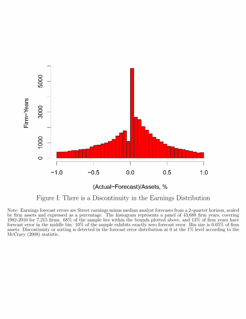
Figure I: There is a Discontinuity in the Earnings Distribution

Note: Earnings forecast errors are Street earnings minus median analyst forecasts from a 2-quarter horizon, scaledby firm assets and expressed as a percentage. The histogram represents a panel of 43,688 firm years, covering1982-2010 for 7,215 firms. 68% of the sample lies within the bounds plotted above, and 13% of firm years haveforecast error in the middle bin. 10% of the sample exhibits exactly zero forecast error. Bin size is 0.05% of firmassets. Discontinuity or sorting is detected in the forecast error distribution at 0 at the 1% level according to theMcCrary (2008) statistic.

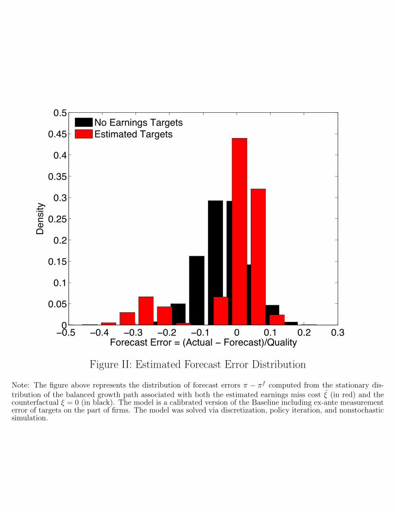
−0.5 −0.4 −0.3 −0.2 −0.1 0 0.1 0.2 0.30

0.05

0.1

0.15

0.2

0.25

0.3

0.35

0.4

0.45

0.5

Forecast Error = (Actual − Forecast)/Quality

Den

sity

No Earnings TargetsEstimated Targets

Student Version of MATLAB

Figure II: Estimated Forecast Error Distribution

Note: The figure above represents the distribution of forecast errors ⇡ � ⇡f computed from the stationary dis-tribution of the balanced growth path associated with both the estimated earnings miss cost ⇠ (in red) and thecounterfactual ⇠ = 0 (in black). The model is a calibrated version of the Baseline including ex-ante measurementerror of targets on the part of firms. The model was solved via discretization, policy iteration, and nonstochasticsimulation.

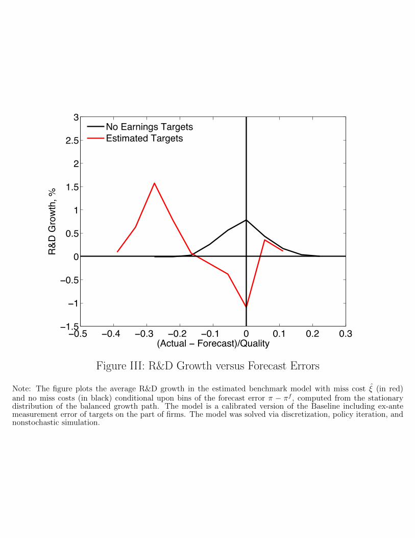
−0.5 −0.4 −0.3 −0.2 −0.1 0 0.1 0.2 0.3−1.5

−1

−0.5

0

0.5

1

1.5

2

2.5

3

(Actual − Forecast)/Quality

R&D

Gro

wth

, %

No Earnings TargetsEstimated Targets

Student Version of MATLAB

Figure III: R&D Growth versus Forecast Errors

Note: The figure plots the average R&D growth in the estimated benchmark model with miss cost ⇠ (in red)and no miss costs (in black) conditional upon bins of the forecast error ⇡ � ⇡f , computed from the stationarydistribution of the balanced growth path. The model is a calibrated version of the Baseline including ex-antemeasurement error of targets on the part of firms. The model was solved via discretization, policy iteration, andnonstochastic simulation.

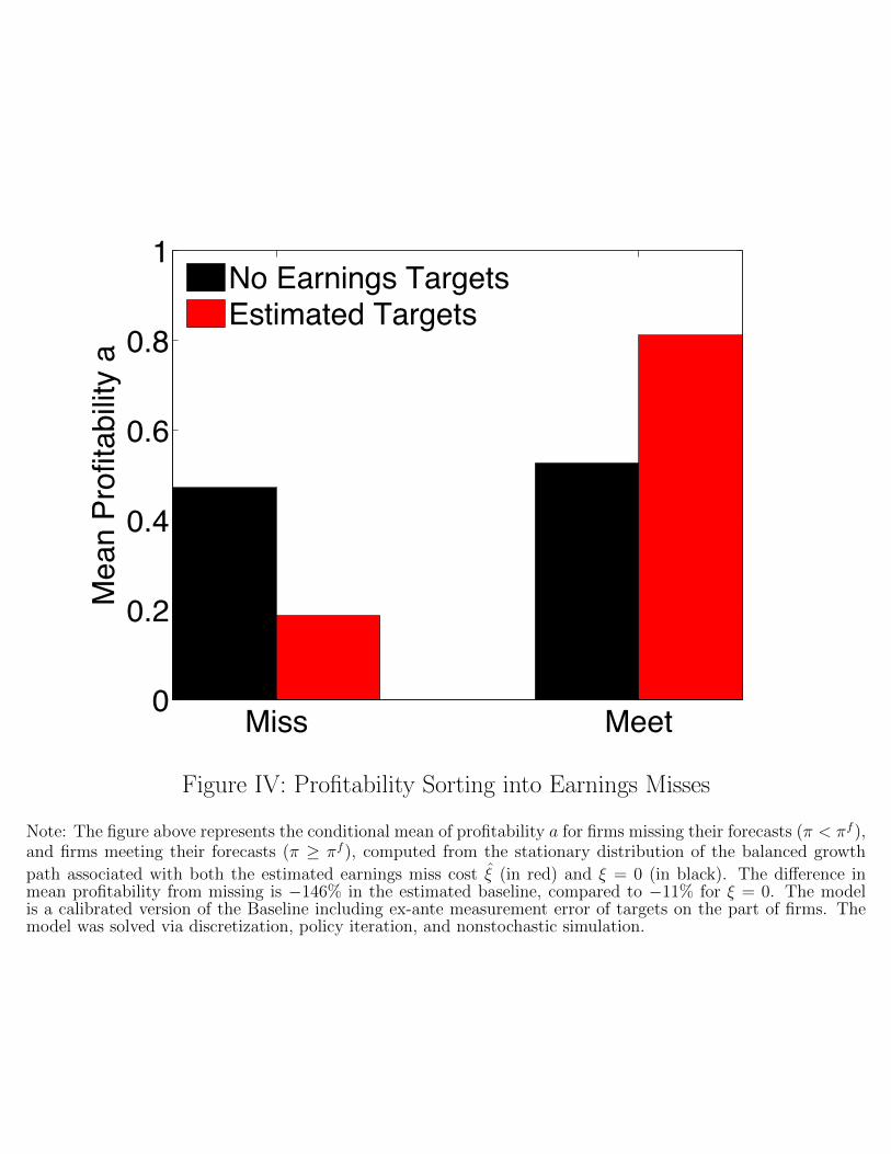
Miss Meet0

0.2

0.4

0.6

0.8

1

Mea

n Pr

ofita

bilit

y a

No Earnings TargetsEstimated Targets

Student Version of MATLAB

Figure IV: Profitability Sorting into Earnings Misses

Note: The figure above represents the conditional mean of profitability a for firms missing their forecasts (⇡ < ⇡f ),and firms meeting their forecasts (⇡ � ⇡f ), computed from the stationary distribution of the balanced growthpath associated with both the estimated earnings miss cost ⇠ (in red) and ⇠ = 0 (in black). The di↵erence inmean profitability from missing is �146% in the estimated baseline, compared to �11% for ⇠ = 0. The modelis a calibrated version of the Baseline including ex-ante measurement error of targets on the part of firms. Themodel was solved via discretization, policy iteration, and nonstochastic simulation.

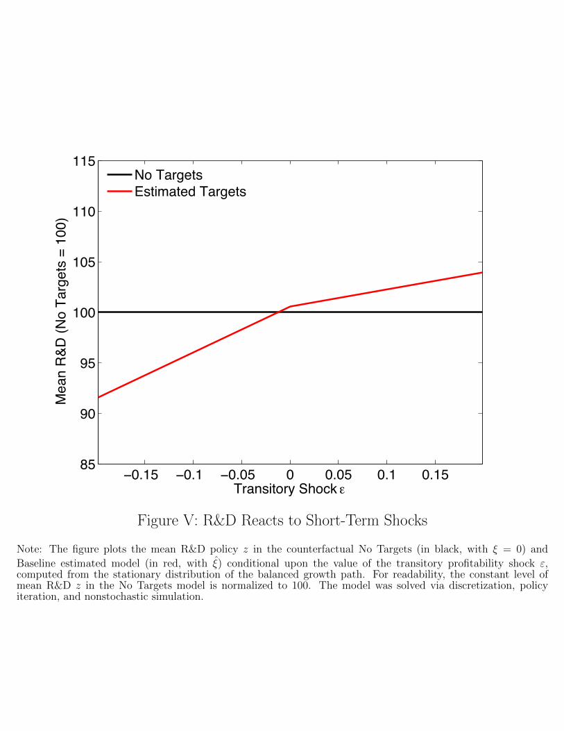
−0.15 −0.1 −0.05 0 0.05 0.1 0.1585

90

95

100

105

110

115

Mea

n R

&D (N

o Ta

rget

s =

100)

Transitory Shock ε

No TargetsEstimated Targets

Student Version of MATLAB

Figure V: R&D Reacts to Short-Term Shocks

Note: The figure plots the mean R&D policy z in the counterfactual No Targets (in black, with ⇠ = 0) andBaseline estimated model (in red, with ⇠) conditional upon the value of the transitory profitability shock ",computed from the stationary distribution of the balanced growth path. For readability, the constant level ofmean R&D z in the No Targets model is normalized to 100. The model was solved via discretization, policyiteration, and nonstochastic simulation.

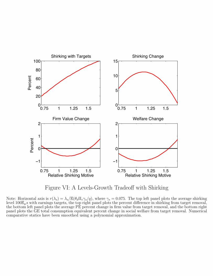
0.75 1 1.25 1.50

20

40

60

80

100Shirking with Targets

Perc

ent

0.75 1 1.25 1.50

5

10

15Shirking Change

0.75 1 1.25 1.5

−1

0

1

2Firm Value Change

Relative Shirking Motive

Perc

ent

0.75 1 1.25 1.5

−1

0

1

2

Relative Shirking Motive

Welfare Change

Student Version of MATLAB

Figure VI: A Levels-Growth Tradeo↵ with Shirking

Note: Horizontal axis is r(�s) = �s/E(✓d⇧v�s/q), where �s = 0.075. The top left panel plots the average shirkinglevel 100Eµs with earnings targets, the top right panel plots the percent di↵erence in shirking from target removal,the bottom left panel plots the average PE percent change in firm value from target removal, and the bottom rightpanel plots the GE total consumption equivalent percent change in social welfare from target removal. Numericalcomparative statics have been smoothed using a polynomial approximation.

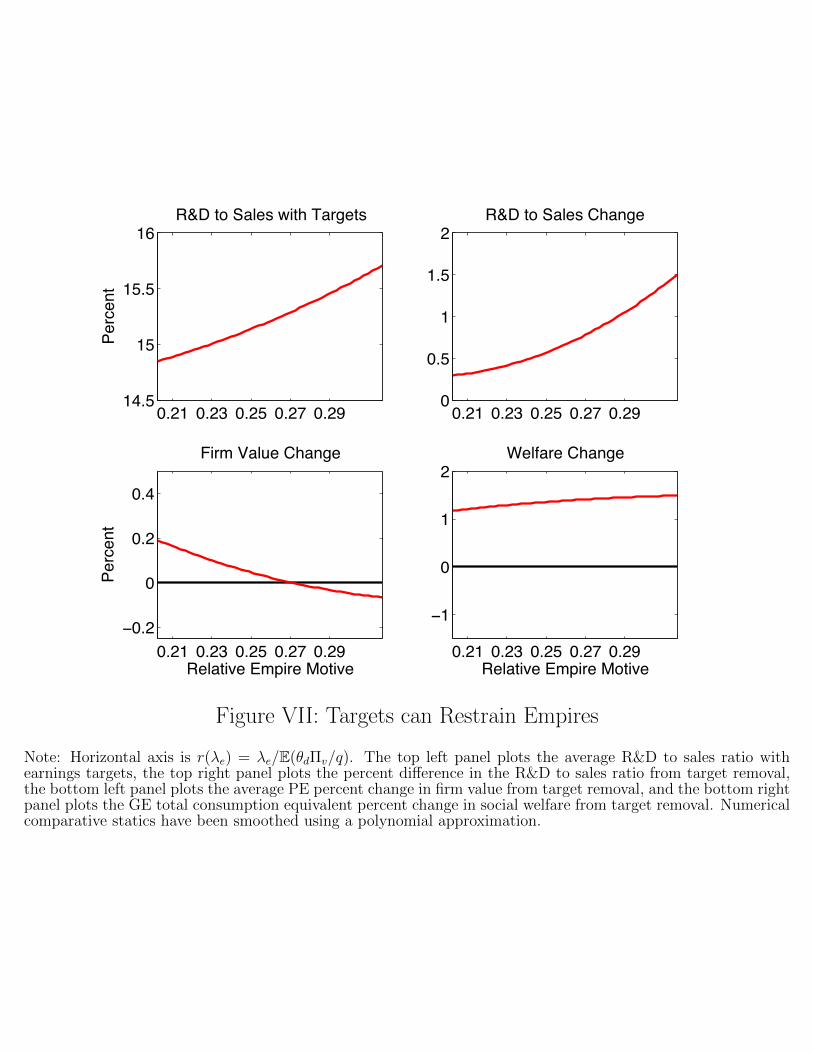
0.21 0.23 0.25 0.27 0.2914.5

15

15.5

16R&D to Sales with Targets

Perc

ent

0.21 0.23 0.25 0.27 0.290

0.5

1

1.5

2R&D to Sales Change

0.21 0.23 0.25 0.27 0.29−0.2

0

0.2

0.4

Relative Empire Motive

Firm Value Change

Perc

ent

0.21 0.23 0.25 0.27 0.29

−1

0

1

2Welfare Change

Relative Empire Motive

Student Version of MATLAB

Figure VII: Targets can Restrain Empires

Note: Horizontal axis is r(�e) = �e/E(✓d⇧v/q). The top left panel plots the average R&D to sales ratio withearnings targets, the top right panel plots the percent di↵erence in the R&D to sales ratio from target removal,the bottom left panel plots the average PE percent change in firm value from target removal, and the bottom rightpanel plots the GE total consumption equivalent percent change in social welfare from target removal. Numericalcomparative statics have been smoothed using a polynomial approximation.

A Data

I combine data from two main sources: 1) the Compustat database for accounting reportsfrom publicly listed US firms, 2) the Institutional Brokers Estimate System (I/B/E/S)database for analyst earnings forecasts and reported earnings for publicly listed US com-panies. Unless otherwise specified, data is at the firm-fiscal year level. Linking table datafrom the CRSP database is also required to connect the I/B/E/S and Compustat datasets,and I make use of CRSP data to compute stock returns where applicable. I also make use ofthe Execucomp database, complementary to Compustat, for executive compensation data.

A.1 Compustat Data

I downloaded Compustat accounting data from the US Fundamentals Annual file in theCRSP/Compustat Merged dataset available throughWharton Research Data Services (WRDS)in January 2014. Allowed linking codes between CRSP and Compustat were “LU” and “LC,”and the following sample restrictions were made:

• Nonmissing total assets at, SIC code sic, book value of capital ppent, GAAP earningsib, operating earnings before depreciation EBITDA oibdp, total sales sale, value ofequity ceq, employment emp

• Positive levels of assets and book value of capital: at, ppent > 0

• No utilities or financial firms as classified by SIC code: sic not in 6000’s or 4900’s

• Fiscal year between 1974 and 2010, from datadate year

• No major mergers flag: compst not equal to “AB”

• Only include primary issue securities: priusa equal to liid

A.2 I/B/E/S Data

I downloaded I/B/E/S earnings forecasts and realized earnings data from WRDS in January2014. My data construction requires files for (stock-split) adjusted detail history, unad-justed detail history, adjusted detail actuals, unadjusted detail actuals, currency headers,and identification headers. I made the following sample restrictions where applicable:

• Nonmissing I/B/E/S permanent ticker ticker, earnings per share (EPS) value of fore-cast or realization value, nonmissing fiscal period end date pends or fpedats, non-missing announcement date anndats, nonmissing analyst and estimator codes analys,estimator

• Only US firms, as indicated in all files by usfirm = 1

• Only firms reporting in US dollars, with available primary/diluted reporting basis flagand historical CUSIP number, as indicated by the currency and identification headerfiles by curr, pdi, cusip

42

I/B/E/S makes available forecasts for earnings per share as well as realized “Street”earnings per share on two reporting bases: “adjusted,” in which the entire time series for asecurity is continuously adjusted for both stock splits and primary/dilution factors, as well as“unadjusted,” in which the originally reported forecasts and actuals are stored. Informationis also available as “summary” or “detail” data, with summary files containing consensusforecasts for a firm as well as reported actuals, rounded to 2 digits (i.e. cents of earnings pershare) and detail files containing the history of analyst forecast rounded to 4 digits.

As Payne and Thomas (2003) note, the joint presence of stock splits and rounding inthe adjusted summary files can lead to a severe loss of information as some earnings hits ormisses are misclassified as zeros due to the ex-post adjustments made by I/B/E/S. Becauseaccurate classification of earnings hits or misses is crucial to my research agenda, I base myanalysis on the unadjusted detail files. However, this requires that all analyst forecasts fromthe unadjusted files be readjusted to the reporting basis as of the earnings announcementdate, since reporting conventions for some securities may change in between a given analystforecast and the earnings announcement.

To readjust analyst forecasts to the same basis as announced unadjusted actuals requiresthe following process:

1. Merge the adjusted detail history files with the unadjusted detail history files, onI/B/E/S variables ticker, fpedats, anndats, analys, estimator

2. For each unadjusted forecast i of EPS for ticker j in fiscal year t

^

EPS

unadj

ijt

as well as

equivalent adjusted forecast ^

EPS

adj

ijt

, compute the stock split ratio of forecast i relativeto the data download date

ratio

i,todayijt

=^

EPS

unadj

ijt

^

EPS

adj

ijt

3. For each unadjusted actual value of EPS for ticker j in fiscal year t EPSunadjjt

, as well as

equivalent adjusted actual EPSadjjt

, compute the stock split ratio of the realized earningsin t relative to the data download date

ratio

t,todayjt

=EPS

unadj

jt

EPS

adj

jt

4. Based on the two ratios above, compute for each unadjusted forecast i of EPS for tickerj in fiscal year t, the EPS forecast ~

EPS

ijt

on the same reporting basis as t

~

EPS

ijt

= ^

EPS

unadj

ijt

ratio

t,todayjt

ratio

i,todayijt

Since they are on the same reporting basis, the analyst forecasts ~

EPS

ijt

, which have4 digit precision, can be directly compared to the unadjusted actuals series EPS

unadj

jt

. Allforecast statistics are computed from these underlying series.

Note that forecasts are made throughout the fiscal year for a given end of year financialrelease. Therefore, I must make a choice of horizon at which to compute earnings forecasts.

43

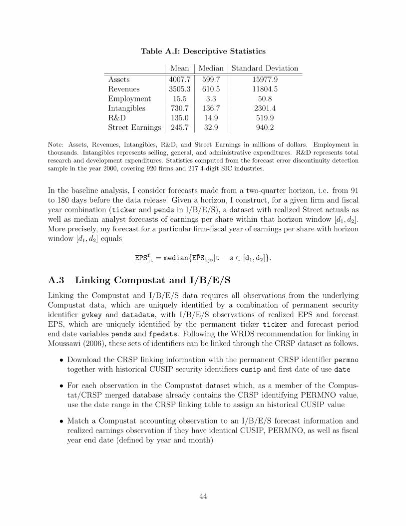
Table A.I: Descriptive Statistics

Mean Median Standard Deviation

Assets 4007.7 599.7 15977.9Revenues 3505.3 610.5 11804.5Employment 15.5 3.3 50.8Intangibles 730.7 136.7 2301.4R&D 135.0 14.9 519.9Street Earnings 245.7 32.9 940.2

Note: Assets, Revenues, Intangibles, R&D, and Street Earnings in millions of dollars. Employment inthousands. Intangibles represents selling, general, and administrative expenditures. R&D represents totalresearch and development expenditures. Statistics computed from the forecast error discontinuity detectionsample in the year 2000, covering 920 firms and 217 4-digit SIC industries.

In the baseline analysis, I consider forecasts made from a two-quarter horizon, i.e. from 91to 180 days before the data release. Given a horizon, I construct, for a given firm and fiscalyear combination (ticker and pends in I/B/E/S), a dataset with realized Street actuals aswell as median analyst forecasts of earnings per share within that horizon window [d

1

, d

2

].More precisely, my forecast for a particular firm-fiscal year of earnings per share with horizonwindow [d

1

, d

2

] equals

EPS

f

jt

= median{ ~

EPS

ijs

|t� s 2 [d1

, d

2

]}.

A.3 Linking Compustat and I/B/E/S

Linking the Compustat and I/B/E/S data requires all observations from the underlyingCompustat data, which are uniquely identified by a combination of permanent securityidentifier gvkey and datadate, with I/B/E/S observations of realized EPS and forecastEPS, which are uniquely identified by the permanent ticker ticker and forecast periodend date variables pends and fpedats. Following the WRDS recommendation for linking inMoussawi (2006), these sets of identifiers can be linked through the CRSP dataset as follows.

• Download the CRSP linking information with the permanent CRSP identifier permnotogether with historical CUSIP security identifiers cusip and first date of use date

• For each observation in the Compustat dataset which, as a member of the Compus-tat/CRSP merged database already contains the CRSP identifying PERMNO value,use the date range in the CRSP linking table to assign an historical CUSIP value

• Match a Compustat accounting observation to an I/B/E/S forecast information andrealized earnings observation if they have identical CUSIP, PERMNO, as well as fiscalyear end date (defined by year and month)

44

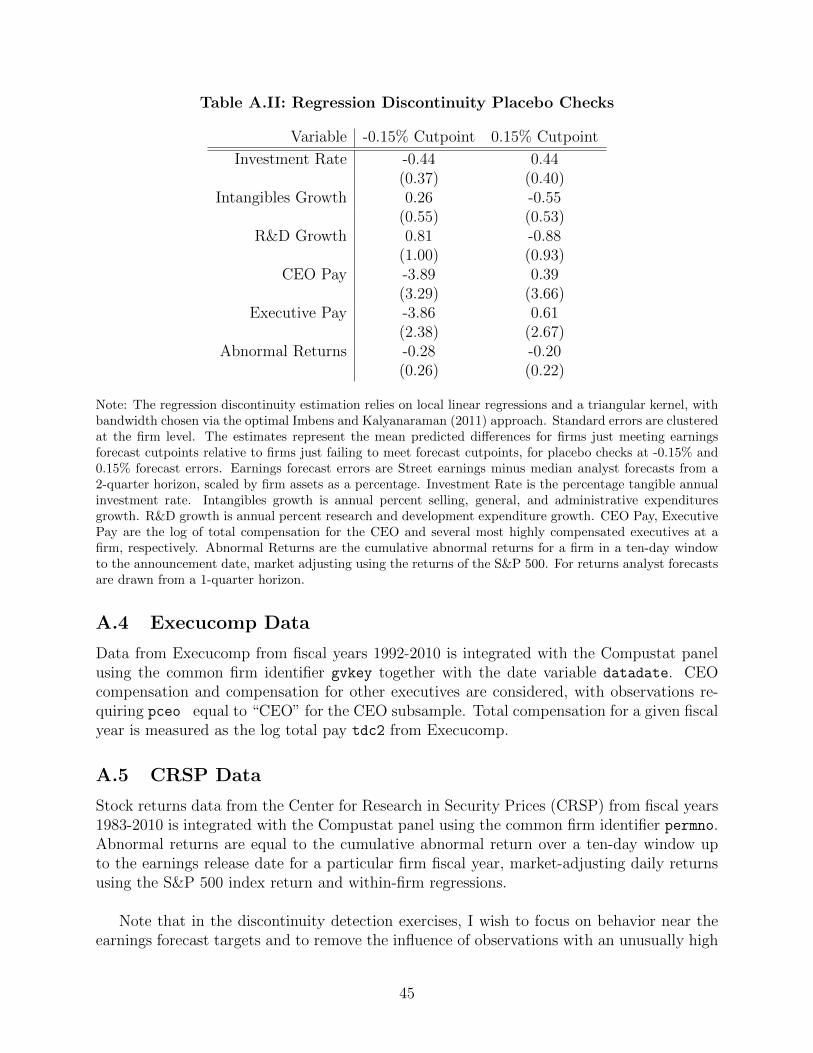
Table A.II: Regression Discontinuity Placebo Checks

Variable -0.15% Cutpoint 0.15% Cutpoint

Investment Rate -0.44 0.44(0.37) (0.40)

Intangibles Growth 0.26 -0.55(0.55) (0.53)

R&D Growth 0.81 -0.88(1.00) (0.93)

CEO Pay -3.89 0.39(3.29) (3.66)

Executive Pay -3.86 0.61(2.38) (2.67)

Abnormal Returns -0.28 -0.20(0.26) (0.22)

Note: The regression discontinuity estimation relies on local linear regressions and a triangular kernel, withbandwidth chosen via the optimal Imbens and Kalyanaraman (2011) approach. Standard errors are clusteredat the firm level. The estimates represent the mean predicted di↵erences for firms just meeting earningsforecast cutpoints relative to firms just failing to meet forecast cutpoints, for placebo checks at -0.15% and0.15% forecast errors. Earnings forecast errors are Street earnings minus median analyst forecasts from a2-quarter horizon, scaled by firm assets as a percentage. Investment Rate is the percentage tangible annualinvestment rate. Intangibles growth is annual percent selling, general, and administrative expendituresgrowth. R&D growth is annual percent research and development expenditure growth. CEO Pay, ExecutivePay are the log of total compensation for the CEO and several most highly compensated executives at afirm, respectively. Abnormal Returns are the cumulative abnormal returns for a firm in a ten-day windowto the announcement date, market adjusting using the returns of the S&P 500. For returns analyst forecastsare drawn from a 1-quarter horizon.

A.4 Execucomp Data

Data from Execucomp from fiscal years 1992-2010 is integrated with the Compustat panelusing the common firm identifier gvkey together with the date variable datadate. CEOcompensation and compensation for other executives are considered, with observations re-quiring pceo equal to “CEO” for the CEO subsample. Total compensation for a given fiscalyear is measured as the log total pay tdc2 from Execucomp.

A.5 CRSP Data

Stock returns data from the Center for Research in Security Prices (CRSP) from fiscal years1983-2010 is integrated with the Compustat panel using the common firm identifier permno.Abnormal returns are equal to the cumulative abnormal return over a ten-day window upto the earnings release date for a particular firm fiscal year, market-adjusting daily returnsusing the S&P 500 index return and within-firm regressions.

Note that in the discontinuity detection exercises, I wish to focus on behavior near theearnings forecast targets and to remove the influence of observations with an unusually high

45

number of analyst forecast records (and potentially dramatic changes in firm news betweenforecast generation and earnings releases). Therefore, before estimating the regression dis-continuities reported in the main text I further restrict the sample to remove observationswith forecast errors greater than than 1% of firm assets in absolute value or with higherthan the 99.5 percentile of forecast frequency in the aggregation period. Table A.I reportsdescriptive statistics on the resulting sample for estimation of the investment regression dis-continuities in Section 2 of the paper. Table A.II reports placebo checks for each of theregression discontinuity estimates reported in Section 2. Table A.III reports block bootstrapestimates of the regression discontinuities from Section 2.

A.6 Data Moments and Model Estimation

To compute model moments, I first require positive values of Compustat sales sale andselling, general, and administrative (SG&A) expenses xsga. Then, I also deflate sales, SG&A,and research and development expenditures xrd by the value of the GDP deflator current asof December 2013.58 Given real vales for a series xt, I compute percentage growth rates as

�xt =

⇢

2xt�xt�1

xt+xt+1, xt 6= 0 or xt�1

6= 0

0, xt = xt�1

= 0.

This measure of growth rates as the di↵erence relative to the average follows Davis andHaltiwanger (1992) and has the advantage of being bounded within [�2, 2]. Selection outof R&D with zero spending for a particular year results in a bounded rather than missinggrowth value. Following the construction of growth rates and real series from Compustatdata, I use the linking process described above to I/B/E/S to obtain a dataset with mergedaccounting (from Compustat) and earnings forecast (from I/B/E/S) data.

After the link, unscaled values of Street earnings (Streetjt

) and forecasts (Streetft

)can be computed by multiplying either the primary or diluted share count as of the fiscalyear end date from Compustat (cshpri or cshfd, respectively, with choice determined byI/B/E/S dilution flag pdi) by the unadjusted earnings per share actual value (EPSunadj

jt

)or forecast value (EPSf

jt

) from I/B/E/S. Once unscaled forecasts and actual Street earningsvalues exist, forecast error is defined as actual Street earnings minus forecast earnings: fe

jt

=Street

jt

� Street

f

jt

.59

58The GDP deflator is given by the series GDPDEF in the Federal Reserve Bank of St. Louis’ online FREDdatabase, accessed at http://research.stlouisfed.org/fred2/.

59I omit the dependence of forecast errors on horizon, although as noted in the I/B/E/S data subsection,earnings per share forecasts are defined as median analyst expectations within a given horizon window beforethe data release date.

46

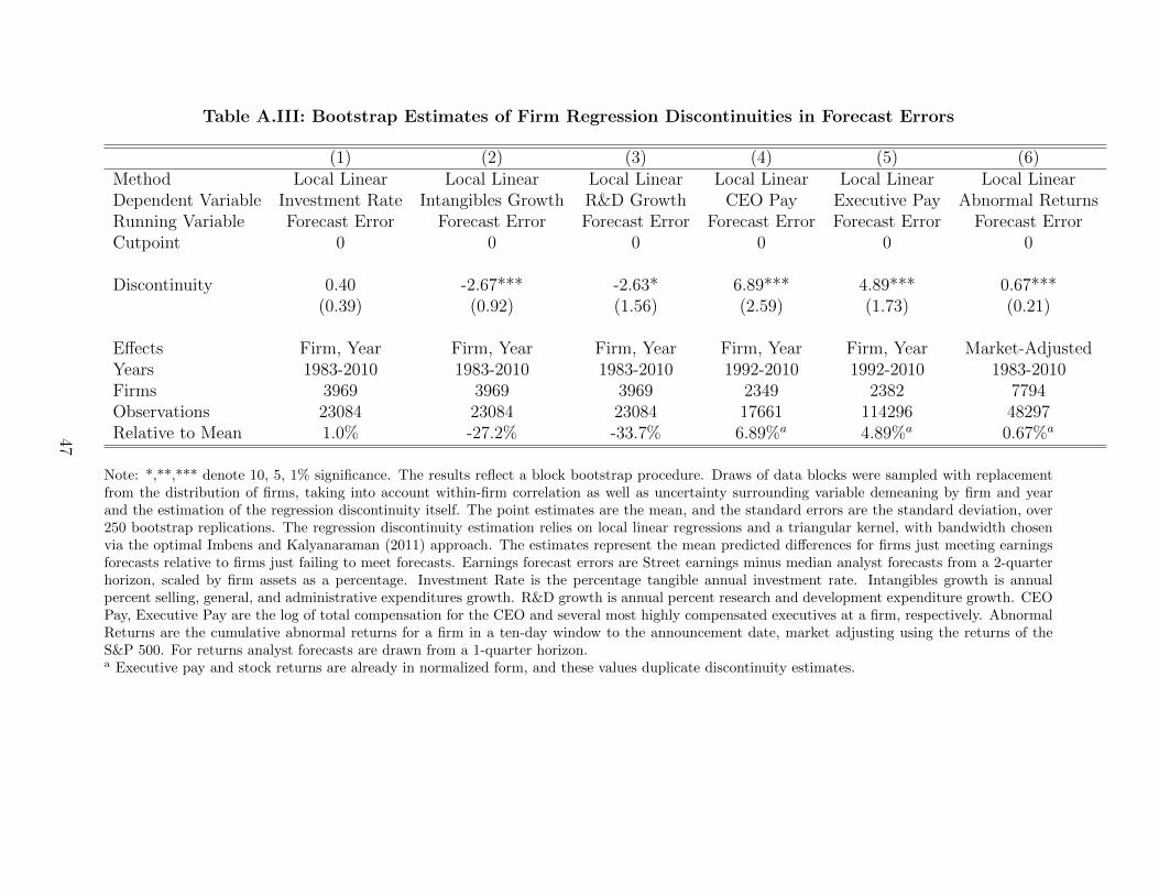
Table A.III: Bootstrap Estimates of Firm Regression Discontinuities in Forecast Errors

(1) (2) (3) (4) (5) (6)Method Local Linear Local Linear Local Linear Local Linear Local Linear Local LinearDependent Variable Investment Rate Intangibles Growth R&D Growth CEO Pay Executive Pay Abnormal ReturnsRunning Variable Forecast Error Forecast Error Forecast Error Forecast Error Forecast Error Forecast ErrorCutpoint 0 0 0 0 0 0

Discontinuity 0.40 -2.67*** -2.63* 6.89*** 4.89*** 0.67***(0.39) (0.92) (1.56) (2.59) (1.73) (0.21)

E↵ects Firm, Year Firm, Year Firm, Year Firm, Year Firm, Year Market-AdjustedYears 1983-2010 1983-2010 1983-2010 1992-2010 1992-2010 1983-2010Firms 3969 3969 3969 2349 2382 7794Observations 23084 23084 23084 17661 114296 48297Relative to Mean 1.0% -27.2% -33.7% 6.89%a 4.89%a 0.67%a

Note: *,**,*** denote 10, 5, 1% significance. The results reflect a block bootstrap procedure. Draws of data blocks were sampled with replacementfrom the distribution of firms, taking into account within-firm correlation as well as uncertainty surrounding variable demeaning by firm and yearand the estimation of the regression discontinuity itself. The point estimates are the mean, and the standard errors are the standard deviation, over250 bootstrap replications. The regression discontinuity estimation relies on local linear regressions and a triangular kernel, with bandwidth chosenvia the optimal Imbens and Kalyanaraman (2011) approach. The estimates represent the mean predicted di↵erences for firms just meeting earningsforecasts relative to firms just failing to meet forecasts. Earnings forecast errors are Street earnings minus median analyst forecasts from a 2-quarterhorizon, scaled by firm assets as a percentage. Investment Rate is the percentage tangible annual investment rate. Intangibles growth is annualpercent selling, general, and administrative expenditures growth. R&D growth is annual percent research and development expenditure growth. CEOPay, Executive Pay are the log of total compensation for the CEO and several most highly compensated executives at a firm, respectively. AbnormalReturns are the cumulative abnormal returns for a firm in a ten-day window to the announcement date, market adjusting using the returns of theS&P 500. For returns analyst forecasts are drawn from a 1-quarter horizon.a Executive pay and stock returns are already in normalized form, and these values duplicate discontinuity estimates.

47

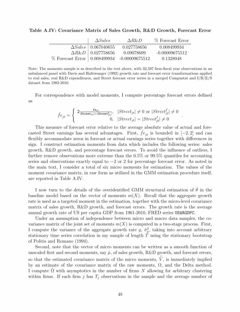
Table A.IV: Covariance Matrix of Sales Growth, R&D Growth, Forecast Error

�Sales �R&D % Forecast Error

�Sales 0.067040655 0.027758656 0.008499934�R&D 0.027758656 0.09078609 -0.00009675512

% Forecast Error 0.008499934 -0.00009675512 0.1328048

Note: The moments sample is as described in the text above, with 32,597 firm-fiscal year observations in anunbalanced panel with Davis and Haltiwanger (1992) growth rate and forecast error transformations appliedto real sales, real R&D expenditures, and Street forecast error series in a merged Compustat and I/B/E/Sdataset from 1982-2010.

For correspondence with model moments, I compute percentage forecast errors definedas

f ejt =

(

2

fe

jt

|Streetjt

|+|Streetfjt

| , |Streetjt| 6= 0 or |Streetfjt| 6= 0

0, |Streetjt| = |Streetfjt| 6= 0.

This measure of forecast error relative to the average absolute value of actual and fore-casted Street earnings has several advantages. First, f ejt is bounded in [�2, 2] and canflexibly accommodate zeros in forecast or actual earnings series together with di↵erences insign. I construct estimation moments from data which includes the following series: salesgrowth, R&D growth, and percentage forecast errors. To avoid the influence of outliers, Ifurther remove observations more extreme than the 0.5% or 99.5% quantiles for accountingseries and observations exactly equal to �2 or 2 for percentage forecast error. As noted inthe main text, I consider a total of six micro moments for estimation. The values of themoment covariance matrix, in raw form as utilized in the GMM estimation procedure itself,are reported in Table A.IV.

I now turn to the details of the overidentified GMM structural estimation of ✓ in thebaseline model based on the vector of moments m(X). Recall that the aggregate growthrate is used as a targeted moment in the estimation, together with the micro-level covariancematrix of sales growth, R&D growth, and forecast errors. The growth rate is the averageannual growth rate of US per capita GDP from 1961-2010, FRED series USARGDPC.

Under an assumption of independence between micro and macro data samples, the co-variance matrix of the joint set of moments m(X) is computed in a two-stage process. First,I compute the variance of the aggregate growth rate g, �2

g , taking into account arbitrarystationary time series correlation in my sample of length T using the stationary bootstrapof Politis and Romano (1994).

Second, note that the vector of micro moments can be written as a smooth function ofunscaled first and second moments, say µ, of sales growth, R&D growth, and forecast errors,

so that the estimated covariance matrix of the micro moments, ˆV , is immediately implied

by an estimate of the covariance matrix of the raw moments, ⌦, and the Delta method.I compute ⌦ with asymptotics in the number of firms N allowing for arbitrary clusteringwithin firms. If each firm j has Tj observations in the sample and the average number of

48

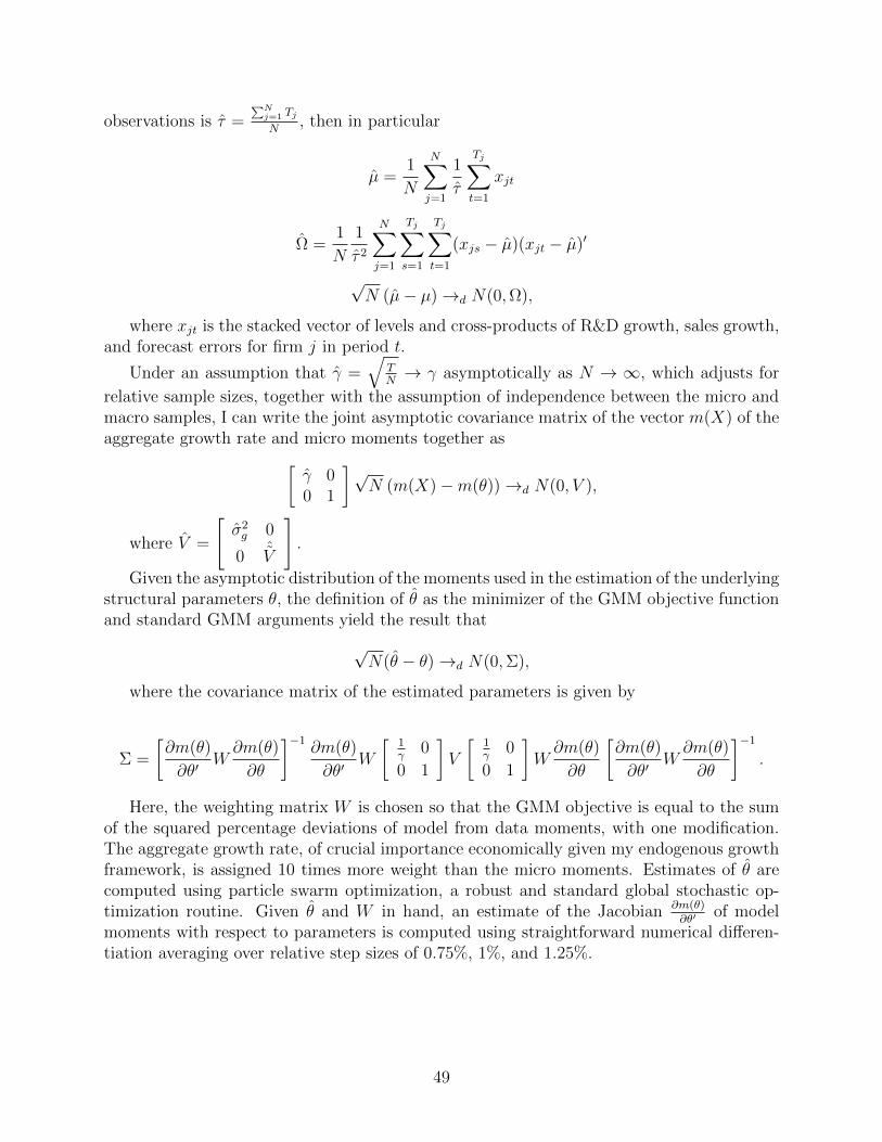
observations is ⌧ =PN

j=1 Tj

N, then in particular

µ =1

N

NX

j=1

1

⌧

TjX

t=1

xjt

⌦ =1

N

1

⌧

2

NX

j=1

TjX

s=1

TjX

t=1

(xjs � µ)(xjt � µ)0

pN (µ� µ) !d N(0,⌦),

where xjt is the stacked vector of levels and cross-products of R&D growth, sales growth,and forecast errors for firm j in period t.

Under an assumption that � =q

TN

! � asymptotically as N ! 1, which adjusts for

relative sample sizes, together with the assumption of independence between the micro andmacro samples, I can write the joint asymptotic covariance matrix of the vector m(X) of theaggregate growth rate and micro moments together as

� 00 1

�pN (m(X)�m(✓)) !d N(0, V ),

where V =

"

�

2

g 0

0 ˆV

#

.

Given the asymptotic distribution of the moments used in the estimation of the underlyingstructural parameters ✓, the definition of ✓ as the minimizer of the GMM objective functionand standard GMM arguments yield the result that

pN(✓ � ✓) !d N(0,⌃),

where the covariance matrix of the estimated parameters is given by

⌃ =

@m(✓)

@✓

0 W

@m(✓)

@✓

��1

@m(✓)

@✓

0 W

1

�0

0 1

�

V

1

�0

0 1

�

W

@m(✓)

@✓

@m(✓)

@✓

0 W

@m(✓)

@✓

��1

.

Here, the weighting matrix W is chosen so that the GMM objective is equal to the sumof the squared percentage deviations of model from data moments, with one modification.The aggregate growth rate, of crucial importance economically given my endogenous growthframework, is assigned 10 times more weight than the micro moments. Estimates of ✓ arecomputed using particle swarm optimization, a robust and standard global stochastic op-timization routine. Given ✓ and W in hand, an estimate of the Jacobian @m(✓)

@✓0 of modelmoments with respect to parameters is computed using straightforward numerical di↵eren-tiation averaging over relative step sizes of 0.75%, 1%, and 1.25%.

49

B Theory

B.1 Model Equilibrium

An equilibrium of the model consists of household consumption and savings policies Ct, Bt+1

,{Sjt}j, final goods firm input policies {Xjt}j, LD

t , intermediate goods firm manager R&D,pricing, accounting manipulation, shirking, and franchise pricing policies {zjt, pjt,mjt, sjt,�

Mjt }j,

intermediate goods firm manager rejection policies {rjt}j, analyst earnings forecasts {⇡fjt}j,

aggregate final output Yt, aggregate intermediate goods expenditures Xt, aggregate account-ing manipulation expenditures ACt, aggregate R&D expenditures Zt, aggregate firm misscosts ⌅firm

t , and lump-sum transfers THHt , TM

t , together with prices Rt+1

, {Pjt}, and wt suchthat the following conditions hold.Household Optimizes

Taking as given wages wt, share prices and dividends {Pjt}j, {Djt}j, and lump-sumtransfers THH

t , the values for household consumption Ct, one-period risk free bond savingsBt+1

, and share purchases in intermediate goods firms {Sjt} maximize household utility:

maxCt,Bt+1,{Sjt}

1X

t=0

⇢

t C1��t

1� �

Ct +Bt+1

+

Z

1

0

PjtSjtdj = RtBt + wtL+

Z

1

0

(Pjt +Djt)Sjt�1

dj + T

HHt .

Final Goods Sector OptimizesTaking as given wages wt and intermediate input prices pjt, the competitive and con-

stant returns to scale final goods sector labor and intermediate input demands LDt , {Xjt}j

maximize profits:

max{Xjt},LD

t

Yt �Z

1

0

pjtXjtdj � wtLDt

Yt =(LD

t )�

(1� �)

Z

1

0

[Qjt(ajt + "jt)(1� �ssjt)]�X

1��jt dj.

Managers OptimizeTaking as given an exogenous endowment of consumption goods CM

Qt, exogenous per-sistent and transitory profitability shocks ajt�1

, "jt�1

, long-term quality level Qjt�1

, previousmanager R&D and paper manipulation choices zjt�1

, mjt�1

, next-period earnings forecasts⇧f

jt, and the previous manager’s take-it-or-leave it price �Mjt�1

for the managerial franchise,each manager j 2 [0, 1] born in period t � 1 must make the end of period t � 1 choicerjt�1

2 {0, 1} to reject (rjt�1

= 1) or accept (rjt�1

= 0) the o↵er of the managerial franchisewhen seeking to maximize period t expected utility, i.e.

rjt�1

= argmaxr

�Rt�Mjt�1

(1�r)+C

MQt+T

Mt +(1�r)Et�1

✓

✓dDjt � ⇠I(⇧jt < ⇧fjt)Qjt

+�eQjt + �ssjtQjt + �

Mjt (1� rjt)

◆

.

Conditional upon accepting the previous manager’s franchise o↵er (rjt�1

= 0), in their

50

second period of life in period t each manager j 2 [0, 1] born in period t � 1 must makeR&D investment, paper manipulation, monopoly pricing, and managerial franchise pricingo↵er choices zjt, mjt, pjt, and �M

jt . These decisions take as given the realization of exogenouspersistent and transitory profitability shock ajt, "jt, long-term quality Qjt, current profitforecast ⇧f

jt, as well as the optimal choice rjt of acceptance or rejection of the managerialfranchise by the next-period manager born in period t. The manager seeks to maximize theirperiod t utility, i.e. they solve the problem

maxzjt,mjt,pjt,sjt,�M

jt

✓

�Rt�Mjt�1

+ C

MQt + T

Mt + ✓dDjt � ⇠I(⇧jt < ⇧f

jt)Qjt

+�eQjt + �ssjtQjt + �

Mjt (1� rjt)

◆

.

From the perspective of the manager, perceived miss costs are a combination ⇠ = ⇠

manager +✓d⇠

firm + (1� ✓d)⇠pay, and dividends net of manager clawback compensation and firm-bornemiss costs are Djt = (1� ⌧c) (⇧v(Qjt, ajt, "jt, pjt)(1� �ssjt)� zjtQjt)� �mm

2

jtQjt.Intermediate Goods Firm Values

Given exogenous persistent and transitory profitability shocks ajt, "jt, long-term qual-ity level Qjt, and analyst forecasts ⇧f

jt, as well as manager-determined intermediate goodsfirm R&D investments zjt, monopoly prices pjt, shirking decisions sjt, and accounting ma-nipulation choices mjt, the value of intermediate goods firms j at time t is given by thepresent-discounted value of firm dividends

E1X

t=0

✓

1

R

◆t ✓ (1� ⌧c) (⇧v(Qjt, ajt, "jt, pjt)(1� �ssjt)� zjtQjt)��mm2

jtQjt � (⇠firm � ⇠

pay)I(⇧Streetjt < ⇧f

jt)Qjt

◆

,

⇧Streetjt = (1� ⌧c) (⇧v(Qjt, ajt, "jt, pjt)(1� �ssjt)� zjtQjt) +mjtQjt

Qjt+1

=

⇢

�Qjt, with probability �(zjt)max(Qjt,!Qt+1

), with probability 1� �(zjt), �(zjt) = Az

↵jt

ajt = (1� ⇢a) + ⇢aajt�1

+ ⇣jt, ⇣jt ⇠ N(0, �2

a), "jt ⇠ N(0, �2

")

⇧v(Qjt, ajt, "jt, pjt) = pjtXjt � Xjt, = 1� �.

Analyst Sector Optimizes

Taking as given normalized Street earnings last period ⇡jt�1

=⇧

Streetjt�1

Qjt�1, an outside analyst

sector forecasts normalized Street earnings ⇡jt today, where the forecast earnings levels

⇡

fjt =

⇧

fjt

Qjtmust minimize analyst loss as follows

⇡

fjt = argmin

⇡fE⇡jt�1(⇡

f � ⇡jt)2

.

Labor and Asset Markets Clear

L

Dt = L (Final Goods Labor Input)

Bt+1

=

Z

�

Mjt (1� rjt�1

)dj (Borrowing for Franchise Purchases Only)

51

Sjt = 1� ✓d (Equity Share Market)

rjt = 0 (Managerial Franchise Market)

Government Budget Balances

T

HHt + T

Mt =

Z

⌧c (⇧vjt(1� �ssjt)� zjtQjt) dj

Managers Consume Their Endowments

C

Mt =

Z

C

Mjt dj = C

MQt

Resource Constraint and Aggregation Conditions are Satisfied

Yt + C

MQt = Ct + C

Mt +Xt + ⌅firm

t + Zt + ACt (Goods Market Clearing)

Xt =

Z

Xjtdj (Intermediate Consumption)

Zt =

Z

zjtQjtdj (R&D Investment)

⌅Firmt =

Z

⇠

firmI(⇧Streetjt < ⇧f

jt)Qjtdj (Firm Earnings Costs)

ACt =

Z

ACm(mjt)Qjtdj (Accounting Manipulation Costs)

B.2 Normalization and Recursive Firm Problem

Consider a stationary balanced growth bath equilibrium where average quality in the econ-omy Qt =

R

Qjtdj grows at a constant rate g and there exists an invariant distribution

µ(ajt, "jt, qjt, ⇡fjt) of intermediate goods firm manager state variables with qjt =

Qjt

Qtand ⇡f

jt

defined above. Then, immediately, all of the aggregates in the economy grow at the rate g

as well, since

Xt =

Z

Xjtdj = Qt

Z

L(ajt + "jt)(1� �ssjt)qjtdµ / Qt

Zt =

Z

zjtQjtdj = Qt

Z

zjtqjtdµ / Qt

⌅firmt =

Z

⇠

firmI(⇧Streetjt < ⇧f

jt)Qjtdj = Qt

Z

⇠

firmI(⇡jt < ⇡

fjt)qjtdµ / Qt

ACt =

Z

�mm2

jtQjtdj = Qt

Z

�mm2

jtqjtdj / Qt

Yt =L

�

(1� �)

Z

1

0

[Qjt(ajt + "jt)(1� �ssjt)]�X

1��jt dj =

L

1� �

Qt

Z

qjt(ajt+"jt)(1��ssjt)dµ / Qt

52

Ct = Yt �Xt � Zt � ACt � ⌅firmt / Qt.

Therefore, the household intertemporal Euler equation for savings in one-period bonds yieldsthe standard result of a constant interest rate Rt+1

= 1

⇢(1+ g)� = R. Note, as will be shown

below, that manager value maximization solves

maxzjt,mjt,sjt

E0

( 1X

t=0

✓

1

R

◆t

D

Mjt

)

= maxzjt,mjt,sjt

E0

( 1X

t=0

✓

1

R

◆t

Qt

D

Mjt

Qt

)

$ maxzjt,mjt,sjt

E0

( 1X

t=0

✓

1 + g

R

◆tD

Mjt

Qt

)

.

The above trivially omits the monopoly pricing decision pjt = 1 from the firm problem. Also,if � � 1 then 1+g

R= ⇢(1+ g)1�� ⇢ < 1. DM

jt , the manager flow return written in full in the

equilibrium above, is homogenous in Qjt and hence stationary since qjt =Qjt

Qtis stationary.

Therefore, the intermediate goods firm manager’s objective exists in stationary, normalizedform.

Manager policies can be obtained as the result of maximization of manager flow returnsdiscounted by the market interest rate, the objective written and analyzed above. To justifythis, first note that manager j born in time t�1 will accept the o↵er of a managerial franchise(i.e. set rjt�1

= 0) for the following period t at price �Mjt�1

if and only if

Rt�Mjt�1

Et�1

✓

✓dDjt � ⇠I(⇧Streetjt < ⇧f

jt)Qjt

+�eQjt + �

Mjt

◆

.

Via backward induction, since �Mjt�1

is a take-it-or-leave it price from the previous managerand since the previous manager’s utility is strictly increasing in �M

jt , it must always be thecase that market clearing for managerial franchises pins down the price �M

jt�1

:

�

Mjt�1

=1

Rt

Et�1

✓

✓dDjt � ⇠I(⇧Streetjt < ⇧f

jt)Qjt

+�eQjt + �ssjtQjt + �

Mjt

◆

.

Repeated forward substitution into the expression for manager consumption in period t

therefore implies that in period t the manager born in t�1 maximizes the present discountedstream of manager utilities from period t onwards, exactly the objective stated in the text.

Note that because they are exogenous to the manager’s linear payo↵s, the managerconsumption endowments C

MQt and transfers T

Mt do not impact manager policies or in-

termediate goods firm values. However, both terms are useful technically. A high enoughvalue of CM ensures that potentially negative dividends and clawbacks ⇠pay do not result innegative manager consumption levels. Meanwhile an appropriate and maintained choice ofT

Mt = �

R

✓dDjtdj+R

⇠

payI(⇧jt < ⇧fjt)Qjtdj ensures that manager consumption on aggregate

is equal to exogenous endowment levels CMQt exactly. Hence, household consumption can

be backed out via the resource constraint, i.e.

Ct = Yt �Xt � ACt � Zt � ⌅firmt ,

53

which is the expression used to argue for Rt = R above.Also, trivially note that the analyst problem yields ⇡f

jt = Eµ(⇡jt|⇡jt�1

) given the meansquared error loss function for analysts. Omitting t and j subscripts for clarity, using 0 todenote future periods, and writing the manager problem recursively yields

V

M(a, ", q, ⇡f ) = maxz,m,s

⇢

✓dd� ⇠I(⇡ < ⇡

f )q + �eq + �ssq +

✓

1 + g

R

◆

EV M(a0, "0, q0, ⇡f 0)

�

d = (1� ⌧c) (�(a+ ")qL(1� �ss)� zq)� �mm2

q

⇡ = (1� ⌧c)(�(a+ ")L(1� �ss)� z) +m

a

0 = (1� ⇢a) + ⇢aa+ ⇣

0, ⇣

0 ⇠ N(0, �2

a), "

0 ⇠ N(0, �2

")

q

0 =

(

�q1+g

, with prob. �(z) = Az

↵

maxn

q1+g

,!

o

, with prob. 1� �(z)

⇡

f 0= Eµ (⇡

0|⇡) .

The stationary, recursive, normalized intermediate goods firm manager problem above fea-tures discounting at rate (1 + g)/R rather than 1/R, and sees “depreciation” of normalizedrelative long-term quality levels q by the rate g each period. The manager problem also al-lows for the influence of corporate taxes, through the ⌧c marginal rate, on firm decisions.60 Inthis form, the problem can be solved using standard numerical dynamic programming tech-niques, as discussed in the Numerical Appendix C below. Also, once optimal policies areobtained, a similar recursive structure obtains for intermediate goods firm values themselvesthrough direct substitution of manager optimal policies.

Now I explicitly define the notion of stationarity which must be satisfied by the distri-bution of normalized state variables µ(a, ", q, ⇡f ). The distribution must be invariant toforward iteration on both the exogenous driving profitability processes a and " as well asthe endogenous forecast and long-term quality transitions. Let z(a, ", q, ⇡f ), m(a, ", q, ⇡f ),and ⇡(a, ", q, ⇡f ) be the optimal R&D policy, optimal accounting manipulation policy, andinduced normalized Street earnings functions, and let fa(a0|a) and f"(") be the transitionand density functions for the exogenous processes. Formally, the stationary distribution µ

satisfies the following condition:

µ(a0, "0, q0, ⇡f 0) =

R

��

z(a, ", q, ⇡f )�

fa(a0|a)f"("0)Ih

q

0 = �q1+g

, ⇡

f 0= E(⇡0|⇡(a, ", q, ⇡f ))

i

dµ(a, ", q, ⇡f )

+R �

1� ��

z(a, ", q, ⇡f )��

fa(a0|a)f"("0)Ih

q = q1+g

, ⇡

f 0= E(⇡0|⇡(a, ", q, ⇡f ))

i

dµ(a, ", q, ⇡f ).

The aggregation condition which must further be satisfied on a stationary balanced growthpath, which guarantees that the aggregate growth rate of long-term quality is generated by

60All numerical results in the paper incorporate income taxation at a marginal 35% rate, but this consid-eration is omitted from the main text for brevity.

54

firm policies and the stationary distribution µ, repeats here from the main text.

1 + g =Q

0

Q

=

R

�(z(a, ", q, ⇡f ))�qdµ(a, ", q, ⇡f )+R

q>!(1+g)(1� �(z(a, ", q, ⇡f )))qdµ(a, ", q, ⇡f )

+R

q!(1+g)(1� �(z(a, ", q, ⇡f )))!(1 + g)dµ(a, ", q, ⇡f )

The first term represents quality growth generated by quality ladder innovation arrivals, thesecond term represents quality growth from lagging-quality firms away from the di↵usionbound !, and the final term represents quality growth from lagging quality firms at thedi↵usion boundary.

Note that the model used for cost estimation in Section 4 imposes �e = �s = sjt = 0 and⇠ = ⇠

manager, i.e. the model assumes away agency conflicts and mechanical resource costs ofearnings misses, while the shirking model in Section 5 assumes �e = 0 and the empire buildingcase in Section 5 assumes �s = sjt = 0. Both models of Section 5 assume ⇠ = (1 � ✓d)⇠pay,i.e. that the costs of earnings misses represent explicit manager compensation policies.

B.3 Welfare and Firm Value Change Formulas

The total consumption equivalent welfare gains from the removal of earnings targets, i.e.moving from ⇠ > 0 ! ⇠ = 0 comparing balanced growth paths only, can be written as 100�where � satisfies the following equation:

1X

t=0

⇢

t (Ct,targets(1 +�))1��

1� �

=1X

t=0

⇢

t (Ct,notargets)1��

1� �

.

All “targets” subscripts refer to cases with ⇠ > 0 and “notargets” subscripts refer to caseswith ⇠ = 0. Trivially, this yields the following formula and decomposition of the welfaregains from removal of the earnings target friction:

� =C

0,notargets

C

0,targets| {z }

Static

✓

1� ⇢(1 + gtargets)1��

1� ⇢(1 + gnotargets)1��

◆

11��

| {z }

Dynamic

.

The above welfare calculations are general equilibrium, in that they take into account allaggregate changes in growth rates, forecasting systems, and the stationary distribution ofthe economy when targets are removed. By contrast, the partial equilibrium change in firmvalue resulting from the removal of earnings targets is computed leaving these quantitiesunchanged, since from the perspective of the firm such aggregates are fixed. The resultingformula for the average change in firm value used in the text is

100Eµtargets log

✓

Vnotargets

Vtargets

◆

.

Note that the text reports in the cost estimation of Section 4 a conservative version of themeasures above which omit the direct e↵ect of the removal of earnings targets costs on the

55

aggregate consumption level and firm value by assuming costs are private to the manager,⇠ = ⇠

manager. Therefore, there is no mechanical e↵ects of the target removal on aggregatehousehold consumption or firm dividends through a resource channel. By contrast Section 5,which assumes that miss costs are based on manager compensation, prevents a mechanicalimpact of miss costs on aggregate consumption through the lump-sum transfers away frommanagers but does allow for clawback to increase firm flow dividends for valuation purposes.

B.4 Adding Measurement Error

The main text shows results for a version of the baseline model with “target measurementerror” ⌫jt for firms. ⌫jt is a transitory white noise disturbance with variance �2

⌫ for firm j

in period t which is unknown at the time manager policies are determined but shifts therealized profits for firms and hence the relevant earnings target. More precisely, this involvesreplacement of the standard intermediate goods firm manager optimization problem fromthe equilibrium definition above with one that incorporates ⌫jt:

maxzjt,mjt,pjt

E( 1X

t=0

✓

1

R

◆t ✓ (1� ⌧c) (⇧v(Qjt, ajt, "jt, pjt)� zjtQjt)��mm2

jtQjt � ⇠I((⇧Streetjt + ⌫jt) < ⇧f

jt)Qjt

◆

)

Qjt+1

=

⇢

�Qjt, with probability �(zjt)max(Qjt,!Qt+1

), with probability 1� �(zjt), �(zjt) = Az

↵jt

ajt = (1� ⇢a) + ⇢aajt�1

+ ⇣jt, ⇣jt ⇠ N(0, �2

a), "jt ⇠ N(0, �2

"), ⌫jt ⇠ N(0, �2

⌫)

In practice, since ⌫ isn’t a state variable for the firm at the time policies are determined,the recursive normalized problem can be modified from the statement above to the followingform:

V

M(a, ", q, ⇡f ) = maxz,m

⇢✓

(1� ⌧c) (�(a+ ")qL� zq)��mm2

q � ⇠E⌫I((⇡ + ⌫) < ⇡

f )q

◆

+

✓

1 + g

R

◆

EV M(a0, "0, q0, ⇡f 0)

�

⇡ = (1� ⌧c)(�(a+ ")L� z) +m

a

0 = (1� ⇢a) + ⇢aa+ ⇣

0, ⇣

0 ⇠ N(0, �2

a), "

0 ⇠ N(0, �2

"), ⌫ ⇠ N(0, �2

⌫)

q

0 =

(

�q1+g

, with prob. �(z) = Az

↵

max{!,q}1+g

, with prob. 1� �(z)

⇡

f 0= Eµ (⇡

0|(⇡ + ⌫)) .

Note that since the measurement error version is only discussed in the context of the costestimation model with �e = �s = s = 0, I omit those terms from the dividend flows aboveand write the earnings miss costs as ⇠, which is simply equal to ⇠/✓d in previous notation.

56

C Numerical Solution

The aggregates of the model which are crucial for the general equilibrium solution includethe growth rate g and the forecast function ⇡

f = Eµ(⇡|⇡�1

). I approximate the forecastfunction with a linear rule ⇡f = ⌘

0

+ ⌘

1

⇡�1

. Comparison of model-implied conditionalexpectations and linear forecasts in Figure C.I, as well as a range of forecast accuracy checkswith extended forecast rules and information sets in Table C.III, indicate that the linearforecast approximation based on lagged earnings is quantitatively reasonable.

Given the forecast rule approximation, the model is solved via a combination of dis-cretization, policy iteration, and nonstochastic simulation, together with an outer loop overaggregates. In other words, the rough solution algorithm, given a parametrization of themodel, consists of:

1. Guess values for the aggregate growth rate g, as well as forecast coe�cients ⌘0

, ⌘

1

.

(a) Solve the normalized, recursive manager Bellman equation stated in Theory Ap-pendix B to some specified tolerance, using discretization of the exogenous pro-cesses as discussed below, discretization of value and policy functions, and Howardpolicy acceleration. Within this step, the manager discounts the future using thegrowth-rate normalization as well as interest rate implied by the guess for g andthe household Euler equation, and earnings targets transition according to theassumed forecast coe�cients on normalized reported Street earnings.

(b) Given a solution to the firm problem, use the nonstochastic simulation approachof Young (2010) to iterate forward on exogenous processes and endogenous tran-sitions until a stationary distribution µ is obtained to some tolerance.

(c) Compute the implied aggregate growth rate g, as well as the implied forecastcoe�cients ⌘

0

, ⌘

1

.

2. If the maximum absolute di↵erences between the guessed and implied growth ratesand forecast coe�cients are less than some predetermined tolerances, the model issolved. If the outer loop has not yet converged, then update either the growth rate(using bisection) or the forecast coe�cients (using dampened fixed-point iteration),until they converge to model-implied values.

Some of the practical choices for numerical implementation are listed in the table below.The model is solved using Fortran with heavy parallelization. Note that when required,forward iterations of endogenous variables required both for distributional iteration as wellas expectations in the manager Bellman equation use linear interpolation in the endogenousvariable.

Note that Table C.II records robustness checks of the earnings target costs estimatesfrom the Baseline in the text to alternative parametrizations or assumptions for the model.Also, Figure C.II displays the ergodic or stationary marginal distributions of model stateand policy variables in the Baseline and No Targets economies.

57

Table C.I: Some Practical Numerical Choices

Object Value Explanation

nq 25 Density of q grid[0.08,12.24] Bounds of q grid

n⇡ 20 Density of ⇡ grid[-0.5,1.5] Bounds of ⇡ grid

na 7 Density of a grid[0.59,1.41] Bounds of a grid

n" 3 Density of " grid[-0.20,20] Bounds of " grid

nz 15 Density of z grid[0.0,0.5] Bounds of z grid

nm 15 Density of m grid[-0.5,0.5] Bounds of m grid

NHoward 250 Number of Howard accelerations"pol 0.0 Tolerance for discretized policy convergence"dist 1e-9 Tolerance for distributional convergence"outer,g 1e-5 Tolerance outer GE loop for g"outer,⌘ 1e-2 Tolerance outer GE loop for ⌘⌘update 0.25 Dampening weight on new values for ⌘

Note: The table above describes some practical numerical choices made to solve the normalized recursivemodel described in the Theory Appendix B. The model is solved with discretization, and the grid boundariesas well as densities are displayed above together with tolerances for the various fixed-points required by themodel and described in the numerical solution overview.

58

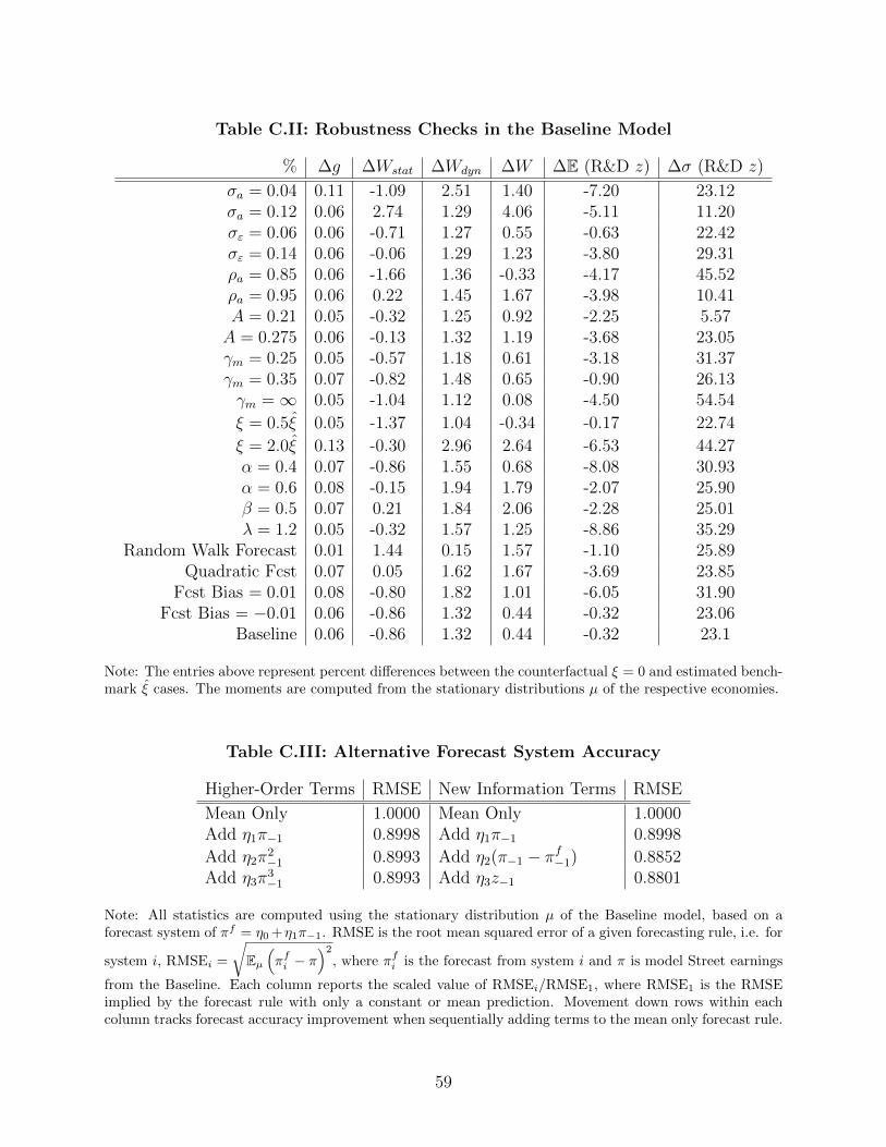
Table C.II: Robustness Checks in the Baseline Model

% �g �Wstat �Wdyn �W �E (R&D z) �� (R&D z)

�a = 0.04 0.11 -1.09 2.51 1.40 -7.20 23.12�a = 0.12 0.06 2.74 1.29 4.06 -5.11 11.20�" = 0.06 0.06 -0.71 1.27 0.55 -0.63 22.42�" = 0.14 0.06 -0.06 1.29 1.23 -3.80 29.31⇢a = 0.85 0.06 -1.66 1.36 -0.33 -4.17 45.52⇢a = 0.95 0.06 0.22 1.45 1.67 -3.98 10.41A = 0.21 0.05 -0.32 1.25 0.92 -2.25 5.57A = 0.275 0.06 -0.13 1.32 1.19 -3.68 23.05�m = 0.25 0.05 -0.57 1.18 0.61 -3.18 31.37�m = 0.35 0.07 -0.82 1.48 0.65 -0.90 26.13�m = 1 0.05 -1.04 1.12 0.08 -4.50 54.54⇠ = 0.5⇠ 0.05 -1.37 1.04 -0.34 -0.17 22.74⇠ = 2.0⇠ 0.13 -0.30 2.96 2.64 -6.53 44.27↵ = 0.4 0.07 -0.86 1.55 0.68 -8.08 30.93↵ = 0.6 0.08 -0.15 1.94 1.79 -2.07 25.90� = 0.5 0.07 0.21 1.84 2.06 -2.28 25.01� = 1.2 0.05 -0.32 1.57 1.25 -8.86 35.29

Random Walk Forecast 0.01 1.44 0.15 1.57 -1.10 25.89Quadratic Fcst 0.07 0.05 1.62 1.67 -3.69 23.85

Fcst Bias = 0.01 0.08 -0.80 1.82 1.01 -6.05 31.90Fcst Bias = �0.01 0.06 -0.86 1.32 0.44 -0.32 23.06

Baseline 0.06 -0.86 1.32 0.44 -0.32 23.1

Note: The entries above represent percent di↵erences between the counterfactual ⇠ = 0 and estimated bench-mark ⇠ cases. The moments are computed from the stationary distributions µ of the respective economies.

Table C.III: Alternative Forecast System Accuracy

Higher-Order Terms RMSE New Information Terms RMSE

Mean Only 1.0000 Mean Only 1.0000Add ⌘

1

⇡�1

0.8998 Add ⌘1

⇡�1

0.8998Add ⌘

2

⇡

2

�1

0.8993 Add ⌘2

(⇡�1

� ⇡

f�1

) 0.8852Add ⌘

3

⇡

3

�1

0.8993 Add ⌘3

z�1

0.8801

Note: All statistics are computed using the stationary distribution µ of the Baseline model, based on aforecast system of ⇡f = ⌘0+⌘1⇡�1. RMSE is the root mean squared error of a given forecasting rule, i.e. for

system i, RMSEi

=

r

Eµ

⇣

⇡

f

i

� ⇡

⌘2, where ⇡f

i

is the forecast from system i and ⇡ is model Street earnings

from the Baseline. Each column reports the scaled value of RMSEi

/RMSE1, where RMSE1 is the RMSEimplied by the forecast rule with only a constant or mean prediction. Movement down rows within eachcolumn tracks forecast accuracy improvement when sequentially adding terms to the mean only forecast rule.

59

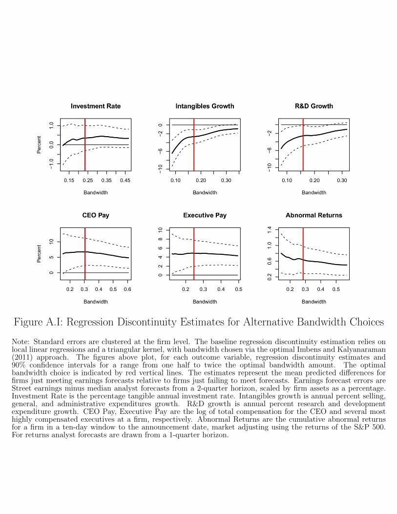
Figure A.I: Regression Discontinuity Estimates for Alternative Bandwidth Choices

Note: Standard errors are clustered at the firm level. The baseline regression discontinuity estimation relies onlocal linear regressions and a triangular kernel, with bandwidth chosen via the optimal Imbens and Kalyanaraman(2011) approach. The figures above plot, for each outcome variable, regression discontinuity estimates and90% confidence intervals for a range from one half to twice the optimal bandwidth amount. The optimalbandwidth choice is indicated by red vertical lines. The estimates represent the mean predicted di↵erences forfirms just meeting earnings forecasts relative to firms just failing to meet forecasts. Earnings forecast errors areStreet earnings minus median analyst forecasts from a 2-quarter horizon, scaled by firm assets as a percentage.Investment Rate is the percentage tangible annual investment rate. Intangibles growth is annual percent selling,general, and administrative expenditures growth. R&D growth is annual percent research and developmentexpenditure growth. CEO Pay, Executive Pay are the log of total compensation for the CEO and several mosthighly compensated executives at a firm, respectively. Abnormal Returns are the cumulative abnormal returnsfor a firm in a ten-day window to the announcement date, market adjusting using the returns of the S&P 500.For returns analyst forecasts are drawn from a 1-quarter horizon.

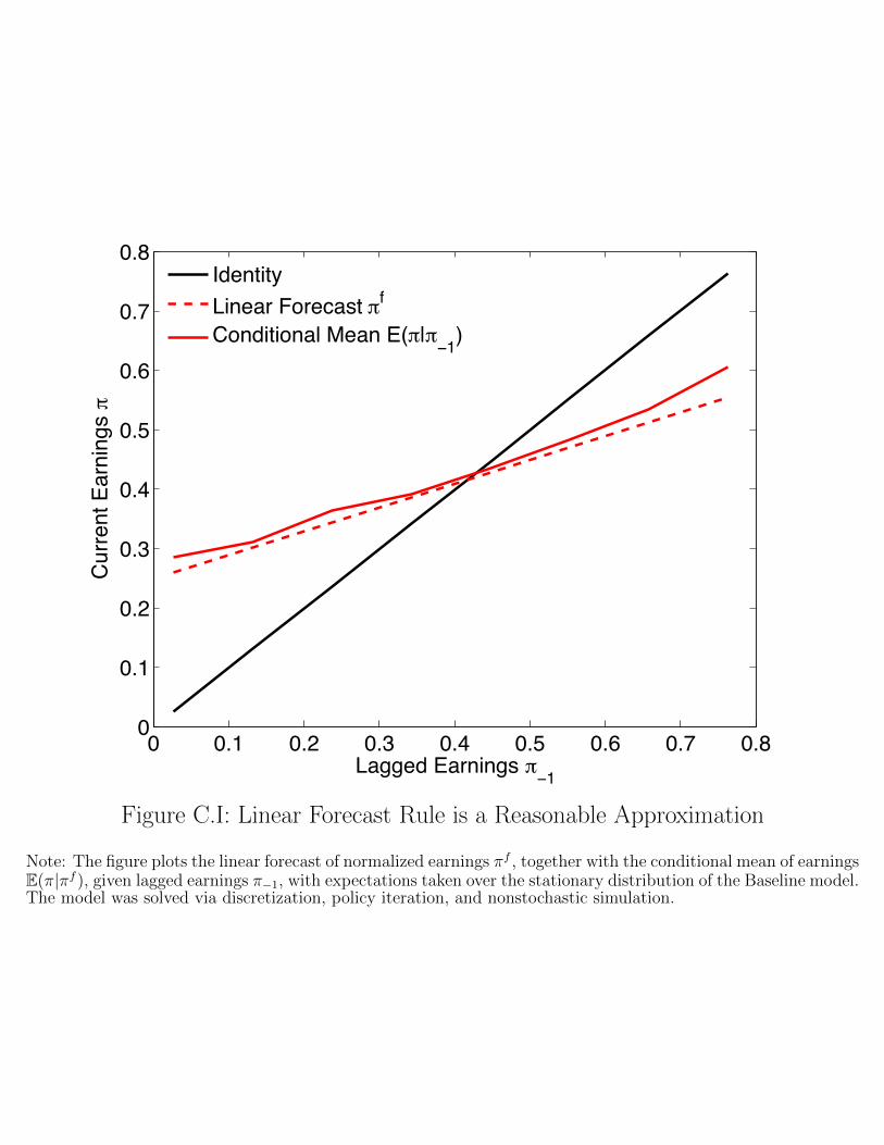
0 0.1 0.2 0.3 0.4 0.5 0.6 0.7 0.80

0.1

0.2

0.3

0.4

0.5

0.6

0.7

0.8

Lagged Earnings π−1

Cur

rent

Ear

ning

s π

IdentityLinear Forecast πf

Conditional Mean E(π|π−1)

Student Version of MATLAB

Figure C.I: Linear Forecast Rule is a Reasonable Approximation

Note: The figure plots the linear forecast of normalized earnings ⇡f , together with the conditional mean of earningsE(⇡|⇡f ), given lagged earnings ⇡�1, with expectations taken over the stationary distribution of the Baseline model.The model was solved via discretization, policy iteration, and nonstochastic simulation.

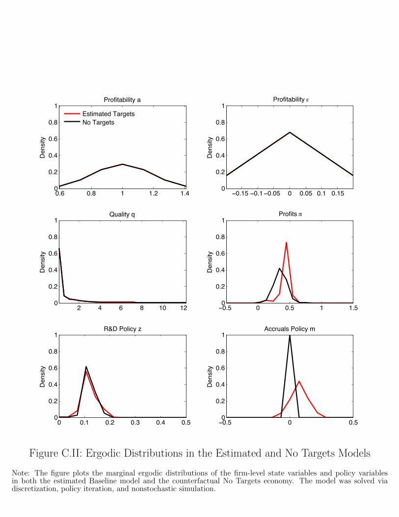
0.6 0.8 1 1.2 1.40

0.2

0.4

0.6

0.8

1Profitability a

Den

sity

Estimated TargetsNo Targets

−0.15 −0.1−0.05 0 0.05 0.1 0.150

0.2

0.4

0.6

0.8

1Profitability ε

Den

sity

2 4 6 8 10 120

0.2

0.4

0.6

0.8

1Quality q

Den

sity

−0.5 0 0.5 1 1.50

0.2

0.4

0.6

0.8

1Profits π

Den

sity

0 0.1 0.2 0.3 0.4 0.50

0.2

0.4

0.6

0.8

1R&D Policy z

Den

sity

−0.5 0 0.50

0.2

0.4

0.6

0.8

1Accruals Policy m

Den

sity

Student Version of MATLAB

Figure C.II: Ergodic Distributions in the Estimated and No Targets Models

Note: The figure plots the marginal ergodic distributions of the firm-level state variables and policy variablesin both the estimated Baseline model and the counterfactual No Targets economy. The model was solved viadiscretization, policy iteration, and nonstochastic simulation.

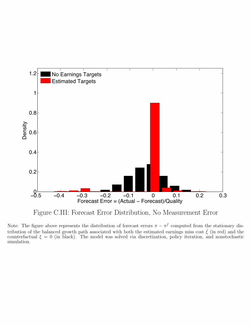
−0.5 −0.4 −0.3 −0.2 −0.1 0 0.1 0.2 0.30

0.2

0.4

0.6

0.8

1

1.2

Forecast Error = (Actual − Forecast)/Quality

Den

sity

No Earnings TargetsEstimated Targets

Student Version of MATLAB

Figure C.III: Forecast Error Distribution, No Measurement Error

Note: The figure above represents the distribution of forecast errors ⇡ � ⇡f computed from the stationary dis-tribution of the balanced growth path associated with both the estimated earnings miss cost ⇠ (in red) and thecounterfactual ⇠ = 0 (in black). The model was solved via discretization, policy iteration, and nonstochasticsimulation.

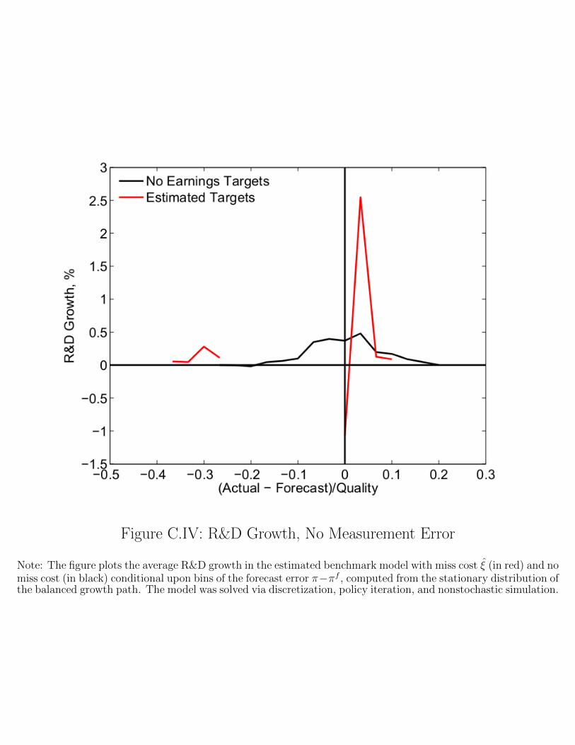
Figure C.IV: R&D Growth, No Measurement Error

Note: The figure plots the average R&D growth in the estimated benchmark model with miss cost ⇠ (in red) and nomiss cost (in black) conditional upon bins of the forecast error ⇡�⇡f , computed from the stationary distribution ofthe balanced growth path. The model was solved via discretization, policy iteration, and nonstochastic simulation.

Miss Meet0

0.2

0.4

0.6

0.8

1

1.2

Mea

n Pr

ofita

bilit

y a

No Earnings TargetsEstimated Targets

Student Version of MATLAB

Figure C.V: Firm Selection, No Measurement Error

Note: The figure above represents the conditional mean of profitability a for firms missing their forecasts (⇡ < ⇡f ),and firms meeting their forecasts (⇡ � ⇡f ), computed from the stationary distribution of the balanced growthpath associated with both the estimated earnings miss cost ⇠ (in red) and ⇠ = 0 (in black). The di↵erence inmean profitability from missing is �193% in the estimated baseline, compared to �25% for ⇠ = 0.

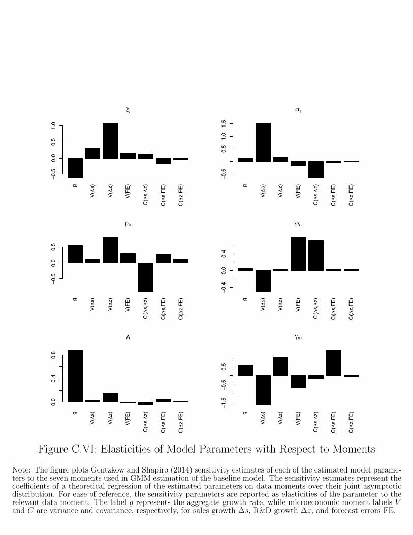
g

V(∆s)

V(∆z)

V(FE

)

C(∆s,∆z)

C(∆s,FE

)

C(∆z,FE

)

ξ

−0.5

0.0

0.5

1.0

g

V(∆s)

V(∆z)

V(FE

)

C(∆s,∆z)

C(∆s,FE

)

C(∆z,FE

)

σε

−0.5

0.5

1.0

1.5

g

V(∆s)

V(∆z)

V(FE

)

C(∆s,∆z)

C(∆s,FE

)

C(∆z,FE

)

ρa

−0.5

0.0

0.5

g

V(∆s)

V(∆z)

V(FE

)

C(∆s,∆z)

C(∆s,FE

)

C(∆z,FE

)

σa−0.4

0.0

0.4

g

V(∆s)

V(∆z)

V(FE

)

C(∆s,∆z)

C(∆s,FE

)

C(∆z,FE

)

A

0.0

0.4

0.8

g

V(∆s)

V(∆z)

V(FE

)

C(∆s,∆z)

C(∆s,FE

)

C(∆z,FE

)

γm

−1.5

−0.5

0.5

Figure C.VI: Elasticities of Model Parameters with Respect to Moments

Note: The figure plots Gentzkow and Shapiro (2014) sensitivity estimates of each of the estimated model parame-ters to the seven moments used in GMM estimation of the baseline model. The sensitivity estimates represent thecoe�cients of a theoretical regression of the estimated parameters on data moments over their joint asymptoticdistribution. For ease of reference, the sensitivity parameters are reported as elasticities of the parameter to therelevant data moment. The label g represents the aggregate growth rate, while microeconomic moment labels Vand C are variance and covariance, respectively, for sales growth �s, R&D growth �z, and forecast errors FE.

0.75 1 1.25 1.50

20

40

60

80

100Shirking with Targets

Perc

ent

0.75 1 1.25 1.50

5

10

15Shirking Change

0.75 1 1.25 1.5

−1

0

1

2Firm Value Change

Relative Shirking Motive

Perc

ent

0.75 1 1.25 1.5

−1

0

1

2

Relative Shirking Motive

Welfare Change

Student Version of MATLAB

Figure C.VII: A Levels-Growth Tradeo↵ with Shirking

Note: Horizontal axis is r(�s) = �s/E(✓d⇧v�s/q), where �s = 0.025. The top left panel plots the average shirkinglevel 100Eµs with earnings targets, the top right panel plots the percent di↵erence in shirking from target removal,the bottom left panel plots the average PE percent change in firm value from target removal, and the bottom rightpanel plots the GE total consumption equivalent percent change in social welfare from target removal. Numericalcomparative statics have been smoothed using a polynomial approximation.