The Macroeconomic Impact of

Money Market Disruptions∗

Fiorella De Fiore†

European Central Bank and CEPR

Marie Hoerova‡

European Central Bank and CEPR

Harald Uhlig§

University of Chicago and CEPR

PRELIMINARY DRAFT

May 16, 2017

Abstract

We build a general equilibrium model featuring unsecured and secured interbank mar-

kets, and collateralized central bank funding. The model is calibrated and used to analyse

the macroeconomic impact of three key developments observed in the European money

markets since 2008: i) the reduced ability of banks to access the unsecured market since

the onset of the global financial crisis and the shift to secured market funding; ii) the

impaired functioning of the secured market during the sovereign crisis; iii) the increased

reliance of banks on central bank funding. We find that disruptions in interbank markets,

as observed during the financial and sovereign debt crises, generate a sizeable impact on

real activity.

∗The views expressed here those of the authors and do not necessarily reflect those of the European CentralBank or the Eurosystem. We are grateful to Joannes Pöschl and Luca Rossi for excellent research assistance.†Directorate General Research, European Central Bank, Postfach 160319, D-60066 Frankfurt am Main.

Email: fiorella.de_fiore@ecb.int. Phone: +49-69-13446330.‡Directorate General Research, European Central Bank, Postfach 160319, D-60066 Frankfurt am Main.

Email: marie_hoerova@ecb.int. Phone: +49-69-13448710.§University of Chicago, Dept. of Economics, 1126 East 59th Street, Chicago, IL 60637. Email: huh-

lig@uchicago.edu. Phone: +1-773-702-3702.

1

1 Introduction

In this paper, we construct a dynamic general equilibrium model featuring heterogeneous

banks, interbank money markets for both secured and unsecured credit, and a central bank

providing funding against collateral. Interbank markets are essential to banks’liquidity man-

agement. They also play a key role in the transmission of monetary policy. These markets

came under severe stress during the global financial crisis of 2007-2009 as well as during the

euro area sovereign debt crisis of 2010-2012.1 We use our model to assess the macroeconomic

impact of the observed interbank market disruptions.

Our modelling approach is motivated by three stylized facts about euro area money markets.

First, interbank money markets are an important funding source for banks in the euro area

but their share in total interbank funding has been diminishing since 2008 (see Figure 1). In

2008, the ratio of interbank liabilities to total assets was about 30%. This ratio started to

decline with the onset of the global financial crisis, dipping below 20% by 2013. This declining

trend reflects disruptions in money markets, with some market segments “freezing”or drying-up

altogether.

Second, there was a dramatic shift away from unsecured and towards secured money market

funding since 2008 (see Figure 2). The secured money market segment was nearly double that

of the unsecured segment in 2008 in terms of the transaction volumes. During the financial

crisis, the share of secured funding grew, as some banks became unable to borrow in the

unsecured markets due to perceptions of increased counterparty risk and shifted to secured

borrowing instead. By 2013, the secured segment was ten times bigger compared to the

unsecured segment.

Third, with private money markets malfunctioning, banks increasingly turned to the central

bank for refinancing (see Figure 3). Reliance on central bank funding gradually rose in the

euro area, particularly with the onset of the sovereign debt crisis. Banks located in euro

area countries with vulnerable sovereigns started borrowing larger amounts from the ECB

and pledging riskier collateral, taking advantage of the more favorable haircuts on risky assets

imposed by the ECB relative to the secured market (see Table 1).

In our model, banks with a liquidity need can obtain funding in the secured or unsecured

market, or at the central bank. Banks face an exogenous probability of being “connected,”

1The failure of the interbank market to redistribute liquidity was highlighted in a number of accounts of therecent crisis (see, for example, Allen and Carletti, 2008, and Brunnermeier, 2009).

defined as the ability to borrow in the unsecured market. Those banks that are unable to

borrow in the unsecured market, the “unconnected”banks, can access the secured market or

central bank funding. To access the secured market or central bank funding banks need to hold

government bonds which can be pledged as collateral. At the beginning of each period, after

knowing whether they are connected or unconnected, banks choose their liabilities (how much

deposit and central bank funding to raise) and their assets (choosing between loans, bonds and

cash). After making their asset-liability choices, banks face idiosyncratic deposit withdrawal

shocks. Banks experiencing low withdrawals can lend funds in the secured or unsecured market.

Banks experiencing high withdrawals can cover them with unsecured borrowing (connected

banks), or the combination of collateralized borrowing and cash buffers (unconnected banks).

All collateralized borrowing is subject to a haircut, which can be different in the private

secured market and at the central bank. If a bank loses access to the unsecured market but

its government bond holdings are suffi ciently valuable, it can replace unsecured funding with

secured funding. Our model can therefore capture the shift from the unsecured to secured

funding observed in the recent years. However, if private counterparties become reluctant to

accept a particular government bond as collateral (due to, e.g., concerns about that sovereign’s

health), access to the secured market will become impaired as well. The possibility that banks

face different haircuts on private and central bank funding allows us to capture the fact that

haircuts set by the central bank can be more favorable in crisis times compared to the private

market haircuts for low-quality collateral. In such circumstances, banks holding such collateral

may replace their lost unsecured and secured funding with borrowing from the central bank.

In our model, the choice between secured market funding and central bank funding is driven

by the comparison of the respective interest rates and haircuts charged in the secured market

and at the central bank.

We calibrate our model using euro area data to quantify the impact of money market dis-

ruptions on the economy. We analyze the macroeconomic impact of three alternative scenarios:

1) reduced access to the unsecured money market; 2) increased haircuts in the secured market,

and 3) increased deposit withdrawals, which were reported in some euro area countries.

Our model suggests that the effects of these market disruptions on investment and output

are sizeable. In the first scenario - when access to the unsecured money market is reduced

- a higher proportion of banks becomes unconnected and needs to satisfy possible deposit

withdrawals by holding bonds and/or money. These banks can therefore invest less in the

2

productive asset, i.e., capital. It is this substitution from investing in productive capital when

connected to investing in unproductive assets when unconnected that generates output effects

of unsecured market disruptions in our model. In our benchmark calibration with moderate

liquidity outflows in the afternoon, unconnected banks are not too much constrained and

shifting from unsecured to secured funcing is only moderately costly. We find that an increase

in the share of unconnected banks from 0.42 (corresponding to the average pre-2008 share of

secured transactions in total volumes) to 0.24 (corresponding to the same average share during

the crisis) generates a decline in output of around 0.4 percent. The adverse impact on real

activity changes substantially if expected liquidity outflows in the afternoon increase with the

disruptions experienced in the unsecured market. If those outflows are expected to double, the

contraction in output is 4 percent.

In the second scenario - when haircuts in the secured market increase - the model economy

moves between two regions. When private haircuts are low and collateral valuable, banks have

access to the private funding markets (either secured or unsecured), and there is no recourse

to central bank funding. When private haircuts increase beyond a certain threshold, banks

relying on secured markets for funding become unable to cover their liquidity needs there as

the value of their collateral drops. They access central bank funding instead. Specifically,

as private haircuts increase, the value of bonds as collateral in the secured market decreases.

Unconnected banks react by holding fewer bonds, raising fewer deposits, and reducing their

investment in capital. Although connected banks maintain their investment in capital broadly

unchanged, the overall effect is a decline in aggregate investment and output. We find that

an increase in private haircuts from 3% to 25% generates an output contraction of 0.3 percent

(0.8 percent if maximum liquidity outflows double). As private haircuts decline further, the

economy moves to the second region where unconnected banks access central bank funding. As

the central bank haircut is stable and more favorable compared to the private market haircut,

banks receive more funding for the same amount of pledged bonds and they can stabilize their

deposit intake and investment. Therefore, the availability of central bank funding puts a floor

to the decline in deposits and capital. The contraction in real activity would be more severe

in the absence of the central bank.

In the third scenario - when banks face increased fears of deposit withdrawals - unconnected

banks react similarly by reducing their deposit, bond and cash holdings. As a result, the

aggregate amount of deposits falls which in turn limits productive investment and reduces the

3

capital stock. We find that doubling the expected maximum share of deposit withdrawals

(from 0.1 to 0.2) generates an output loss of 3 percent.2

This paper is related to the literature on interbank markets and on the impact of sov-

ereign risk on the macroeconomy. There is an extensive literature in banking on the role

of interbank markets in banks’ liquidity management, starting with Bhattacharya and Gale

(1987). A number of recent papers focus on analyzing frictions that prevent interbank markets

from distributing liquidity effi ciently within the banking system. Frictions include asymmetric

information about banks’ assets (Flannery, 1996, Freixas and Jorge, 2007, Heider, Hoerova

and Holthausen, 2015), imperfect cross-border information (Freixas and Holthausen, 2005),

banks’free-riding on liquidity provision by the central bank (Repullo, 2005), and multiplicity

of Pareto-ranked equilibria (Freixas, Martin and Skeie, 2011). Papers in this strand of liter-

ature tend to be partial equilibrium and static, with links to the real economy modeled in a

reduced-form fashion.

Several recent papers build dynamic general equilibrium models which include interbank

trade. For example, Afonso and Lagos (2015) develop an OTC model of the unsecured (Federal

Funds) market and use it to study the intraday evolution of the distribution of reserve balances.

Atkeson, Eisfeldt, and Weill (2015) analyse the trading decisions of banks in an OTC market

and draw implications for policy. Bianchi and Bigio (2014) build a framework to study the

implementation of monetary policy through the banking system. Bruche and Suarez (2009)

show that unsecured interbank market freezes generate large output losses in the presence

of deposit insurance, due to a distorted allocation of credit. Our paper contributes to this

literature by considering both unsecured and secured interbank markets, and collateralized

lending by the central bank.3 In our setup, disruptions in the unsecured money market segment

may in principle be offset by an increased recourse to private secured markets or to central bank

funding. We nevertheless find that disruptions in the unsecured market segment can generate

sizable output costs. When also the secured market segment is severely malfunctioning, the

possibility to tap into central bank can improve macroeconomic outcomes.

In our model, lending from the central bank is backed by government bonds, and increase

in haircuts on sovereign bonds capture in a reduced-form the impact of sovereign default risk

2See, e.g., “Worrying about a Greek bank run,” Reuters, April 15, 2010, http://blogs.reuters.com/felix-salmon/2010/04/15/worrying-about-a-greek-bank-run/.

3A related paper to ours is Schneider and Piazzesi (2017) which builds a framework where banks use reservesto settle interbank trades and to handle endusers’ payment instructions. The authors show that key to theeffi ciency of a payment system is the provision and allocation of collateral.

4

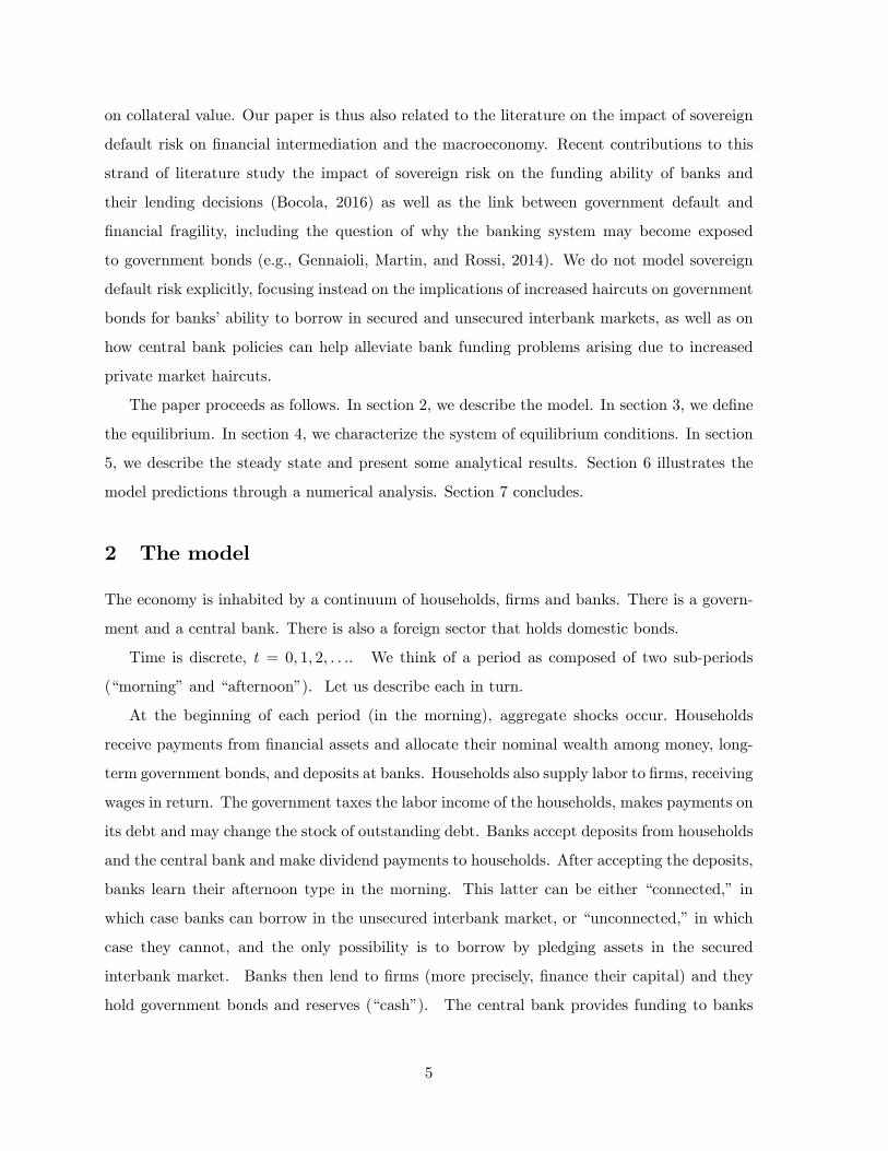
on collateral value. Our paper is thus also related to the literature on the impact of sovereign

default risk on financial intermediation and the macroeconomy. Recent contributions to this

strand of literature study the impact of sovereign risk on the funding ability of banks and

their lending decisions (Bocola, 2016) as well as the link between government default and

financial fragility, including the question of why the banking system may become exposed

to government bonds (e.g., Gennaioli, Martin, and Rossi, 2014). We do not model sovereign

default risk explicitly, focusing instead on the implications of increased haircuts on government

bonds for banks’ability to borrow in secured and unsecured interbank markets, as well as on

how central bank policies can help alleviate bank funding problems arising due to increased

private market haircuts.

The paper proceeds as follows. In section 2, we describe the model. In section 3, we define

the equilibrium. In section 4, we characterize the system of equilibrium conditions. In section

5, we describe the steady state and present some analytical results. Section 6 illustrates the

model predictions through a numerical analysis. Section 7 concludes.

2 The model

The economy is inhabited by a continuum of households, firms and banks. There is a govern-

ment and a central bank. There is also a foreign sector that holds domestic bonds.

Time is discrete, t = 0, 1, 2, . . .. We think of a period as composed of two sub-periods

(“morning”and “afternoon”). Let us describe each in turn.

At the beginning of each period (in the morning), aggregate shocks occur. Households

receive payments from financial assets and allocate their nominal wealth among money, long-

term government bonds, and deposits at banks. Households also supply labor to firms, receiving

wages in return. The government taxes the labor income of the households, makes payments on

its debt and may change the stock of outstanding debt. Banks accept deposits from households

and the central bank and make dividend payments to households. After accepting the deposits,

banks learn their afternoon type in the morning. This latter can be either “connected,” in

which case banks can borrow in the unsecured interbank market, or “unconnected,”in which

case they cannot, and the only possibility is to borrow by pledging assets in the secured

interbank market. Banks then lend to firms (more precisely, finance their capital) and they

hold government bonds and reserves (“cash”). The central bank provides funding to banks

5

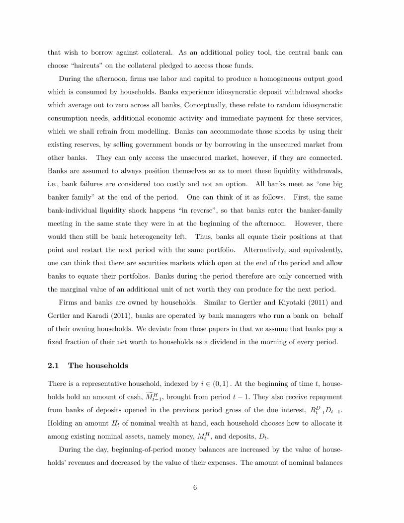
that wish to borrow against collateral. As an additional policy tool, the central bank can

choose “haircuts”on the collateral pledged to access those funds.

During the afternoon, firms use labor and capital to produce a homogeneous output good

which is consumed by households. Banks experience idiosyncratic deposit withdrawal shocks

which average out to zero across all banks, Conceptually, these relate to random idiosyncratic

consumption needs, additional economic activity and immediate payment for these services,

which we shall refrain from modelling. Banks can accommodate those shocks by using their

existing reserves, by selling government bonds or by borrowing in the unsecured market from

other banks. They can only access the unsecured market, however, if they are connected.

Banks are assumed to always position themselves so as to meet these liquidity withdrawals,

i.e., bank failures are considered too costly and not an option. All banks meet as “one big

banker family” at the end of the period. One can think of it as follows. First, the same

bank-individual liquidity shock happens “in reverse”, so that banks enter the banker-family

meeting in the same state they were in at the beginning of the afternoon. However, there

would then still be bank heterogeneity left. Thus, banks all equate their positions at that

point and restart the next period with the same portfolio. Alternatively, and equivalently,

one can think that there are securities markets which open at the end of the period and allow

banks to equate their portfolios. Banks during the period therefore are only concerned with

the marginal value of an additional unit of net worth they can produce for the next period.

Firms and banks are owned by households. Similar to Gertler and Kiyotaki (2011) and

Gertler and Karadi (2011), banks are operated by bank managers who run a bank on behalf

of their owning households. We deviate from those papers in that we assume that banks pay a

fixed fraction of their net worth to households as a dividend in the morning of every period.

2.1 The households

There is a representative household, indexed by i ∈ (0, 1) . At the beginning of time t, house-

holds hold an amount of cash, MHt−1, brought from period t− 1. They also receive repayment

from banks of deposits opened in the previous period gross of the due interest, RDt−1Dt−1.

Holding an amount Ht of nominal wealth at hand, each household chooses how to allocate it

among existing nominal assets, namely money, MHt , and deposits, Dt.

During the day, beginning-of-period money balances are increased by the value of house-

holds’revenues and decreased by the value of their expenses. The amount of nominal balances

6

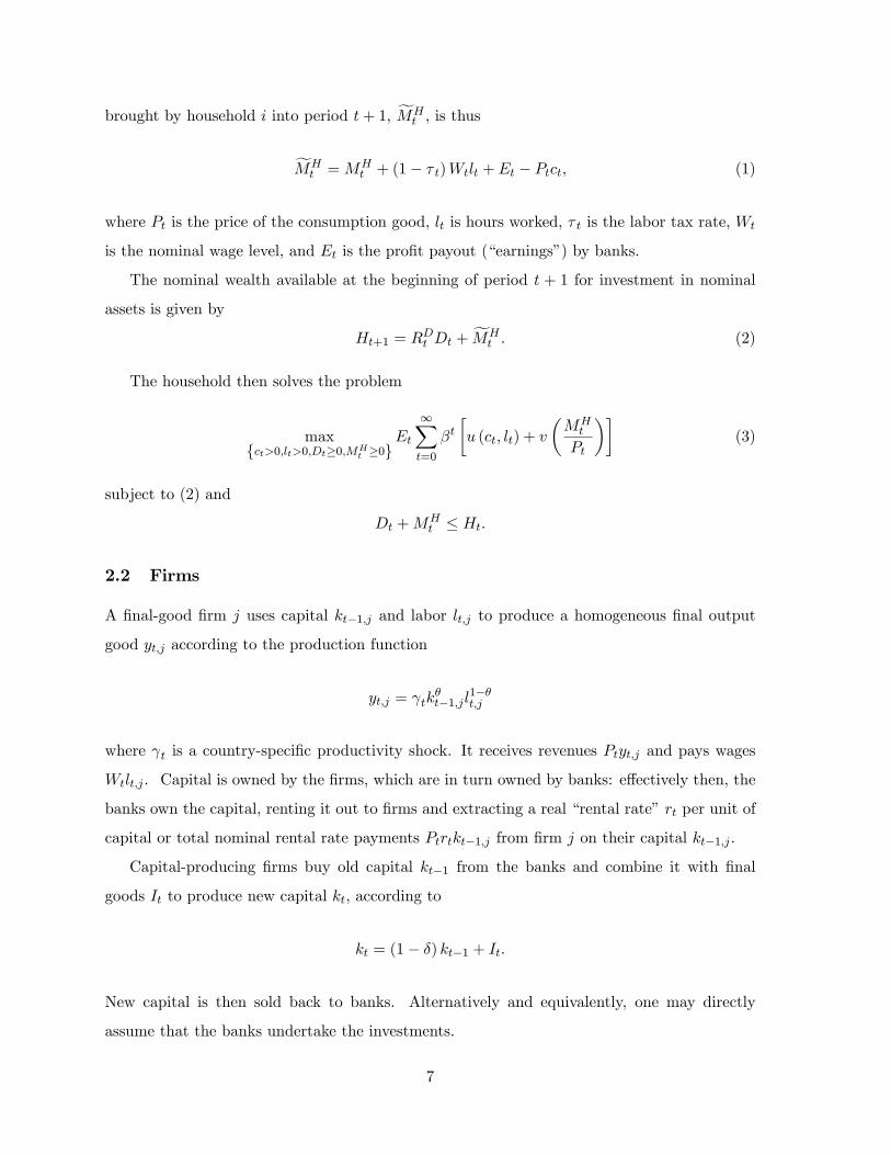
brought by household i into period t+ 1, MHt , is thus

MHt = MH

t + (1− τ t)Wtlt + Et − Ptct, (1)

where Pt is the price of the consumption good, lt is hours worked, τ t is the labor tax rate, Wt

is the nominal wage level, and Et is the profit payout (“earnings”) by banks.

The nominal wealth available at the beginning of period t + 1 for investment in nominal

assets is given by

Ht+1 = RDt Dt + MHt . (2)

The household then solves the problem

max{ct>0,lt>0,Dt≥0,MH

t ≥0}Et

∞∑t=0

βt[u (ct, lt) + v

(MHt

Pt

)](3)

subject to (2) and

Dt +MHt ≤ Ht.

2.2 Firms

A final-good firm j uses capital kt−1,j and labor lt,j to produce a homogeneous final output

good yt,j according to the production function

yt,j = γtkθt−1,jl

1−θt,j

where γt is a country-specific productivity shock. It receives revenues Ptyt,j and pays wages

Wtlt,j . Capital is owned by the firms, which are in turn owned by banks: effectively then, the

banks own the capital, renting it out to firms and extracting a real “rental rate”rt per unit of

capital or total nominal rental rate payments Ptrtkt−1,j from firm j on their capital kt−1,j .

Capital-producing firms buy old capital kt−1 from the banks and combine it with final

goods It to produce new capital kt, according to

kt = (1− δ) kt−1 + It.

New capital is then sold back to banks. Alternatively and equivalently, one may directly

assume that the banks undertake the investments.

7

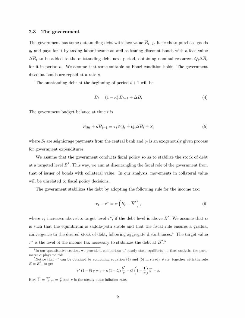
2.3 The government

The government has some outstanding debt with face value Bt−1. It needs to purchase goods

gt and pays for it by taxing labor income as well as issuing discount bonds with a face value

∆Bt to be added to the outstanding debt next period, obtaining nominal resources Qt∆Bt

for it in period t. We assume that some suitable no-Ponzi condition holds. The government

discount bonds are repaid at a rate κ.

The outstanding debt at the beginning of period t+ 1 will be

Bt = (1− κ)Bt−1 + ∆Bt (4)

The government budget balance at time t is

Ptgt + κBt−1 = τ tWtlt +Qt∆Bt + St (5)

where St are seigniorage payments from the central bank and gt is an exogenously given process

for government expenditures.

We assume that the government conducts fiscal policy so as to stabilize the stock of debt

at a targeted level B∗. This way, we aim at disentangling the fiscal role of the government from

that of issuer of bonds with collateral value. In our analysis, movements in collateral value

will be unrelated to fiscal policy decisions.

The government stabilizes the debt by adopting the following rule for the income tax:

τ t − τ∗ = α(Bt −B

∗), (6)

where τ t increases above its target level τ∗, if the debt level is above B∗. We assume that α

is such that the equilibrium is saddle-path stable and that the fiscal rule ensures a gradual

convergence to the desired stock of debt, following aggregate disturbances.4 The target value

τ∗ is the level of the income tax necessary to stabilizes the debt at B∗.5

4 In our quantitative section, we provide a comparison of steady state equilibria: in that analysis, the para-meter α plays no role.

5Notice that τ∗ can be obtained by combining equation (4) and (5) in steady state, together with the ruleB = B

∗, to get

τ∗ (1− θ) y = g + κ (1−Q)b∗

π−Q

(1− 1

π

)b∗ − s.

Here b∗= B

∗

P, s = S

Pand π is the steady state inflation rate.

8

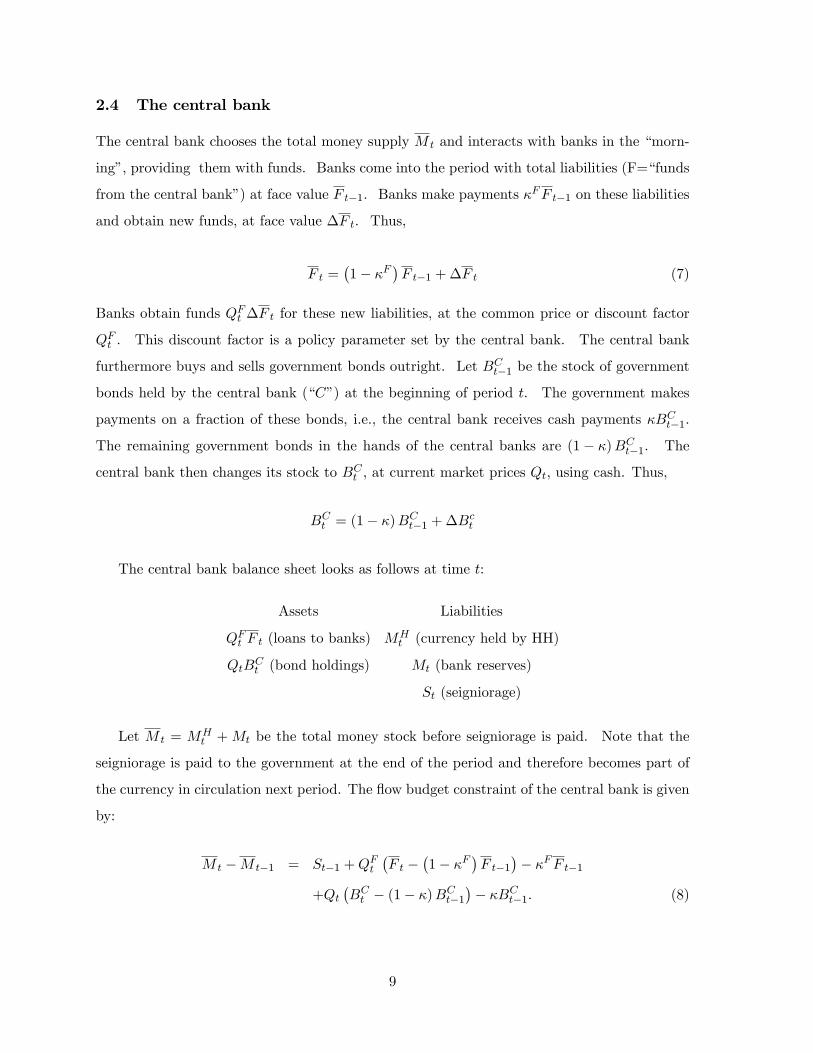
2.4 The central bank

The central bank chooses the total money supply M t and interacts with banks in the “morn-

ing”, providing them with funds. Banks come into the period with total liabilities (F=“funds

from the central bank”) at face value F t−1. Banks make payments κFF t−1 on these liabilities

and obtain new funds, at face value ∆F t. Thus,

F t =(1− κF

)F t−1 + ∆F t (7)

Banks obtain funds QFt ∆F t for these new liabilities, at the common price or discount factor

QFt . This discount factor is a policy parameter set by the central bank. The central bank

furthermore buys and sells government bonds outright. Let BCt−1 be the stock of government

bonds held by the central bank (“C”) at the beginning of period t. The government makes

payments on a fraction of these bonds, i.e., the central bank receives cash payments κBCt−1.

The remaining government bonds in the hands of the central banks are (1− κ)BCt−1. The

central bank then changes its stock to BCt , at current market prices Qt, using cash. Thus,

BCt = (1− κ)BC

t−1 + ∆Bct

The central bank balance sheet looks as follows at time t:

Assets Liabilities

QFt F t (loans to banks) MHt (currency held by HH)

QtBCt (bond holdings) Mt (bank reserves)

St (seigniorage)

Let M t = MHt + Mt be the total money stock before seigniorage is paid. Note that the

seigniorage is paid to the government at the end of the period and therefore becomes part of

the currency in circulation next period. The flow budget constraint of the central bank is given

by:

M t −M t−1 = St−1 +QFt(F t −

(1− κF

)F t−1

)− κFF t−1

+Qt(BCt − (1− κ)BC

t−1)− κBC

t−1. (8)

9

Seigniorage can then be calculated as the residual balance sheet profit,

St = QFt F t +QtBCt −M t. (9)

2.5 Banks

There is a continuum of banks (“Lenders”), indexed by l ∈ (0, 1). Consider a bank l.

2.5.1 Assets and liabilities

At the end of the morning, after earning income on its assets, paying interest on its liabilities

and retrading, but just before paying dividends to share holders, the bank holds four type of

assets. It additionally and briefly holds an asset in the afternoon, for a total of five. As an

overview, the end-of-morning balance sheet of that bank is

Assets Liabilities

Ptkt,l(capital held) Dt,l (deposits by HH)

QtBt,l (bond holdings) QFt Ft,l (secured loans)

Et,l(cash dividends) Nt,l (net worth)

Mt,l(cash reserves)

In detail:

1. Capital kt,l of firms, or, equivalently, firms, who in turn own the capital. Capital can

only be acquired and traded in the morning. Capital evolves according to

kt,l = (1− δ) kt−1,l + ∆kt,l

where ∆kt,l is the gross investment of bank l in capital.

2. Bonds with a nominal face value Bt,l. A fraction κ of the government debt will be repaid.

The bank changes its government bond position per market purchases or sales (“-”) ∆Bt,l

in the morning, so that

Bt,l = (1− κ)Bt−1,l + ∆Bt,l

at the end of the morning. If the bank purchases (sells) bonds on the open market, it

pays (receives) Qt∆Bt,l. As a baseline, we allow ∆Bt,l to be negative, indicating a sale.

10

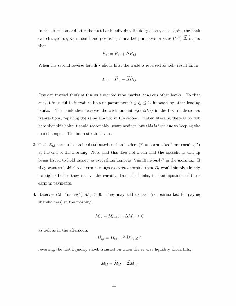
In the afternoon and after the first bank-individual liquidity shock, once again, the bank

can change its government bond position per market purchases or sales (“-”) ∆Bt,l, so

that

Bt,l = Bt,l + ∆Bt,l

When the second reverse liquidity shock hits, the trade is reversed as well, resulting in

Bt,l = Bt,l − ∆Bt,l

One can instead think of this as a secured repo market, vis-a-vis other banks. To that

end, it is useful to introduce haircut parameters 0 ≤ ηt ≤ 1, imposed by other lending

banks. The bank then receives the cash amount ηtQt∆Bt,l in the first of these two

transactions, repaying the same amount in the second. Taken literally, there is no risk

here that this haircut could reasonably insure against, but this is just due to keeping the

model simple. The interest rate is zero.

3. Cash Et,l earmarked to be distributed to shareholders (E = “earmarked”or “earnings”)

at the end of the morning. Note that this does not mean that the households end up

being forced to hold money, as everything happens “simultaneously”in the morning. If

they want to hold those extra earnings as extra deposits, then Dt would simply already

be higher before they receive the earnings from the banks, in “anticipation” of these

earning payments.

4. Reserves (M=“money”) Mt,l ≥ 0. They may add to cash (not earmarked for paying

shareholders) in the morning,

Mt,l = Mt−1,l + ∆Mt,l ≥ 0

as well as in the afternoon,

Mt,l = Mt,l + ∆M t,l ≥ 0

reversing the first-liquidity-shock transaction when the reverse liquidity shock hits,

Mt,l = Mt,l − ∆M t,l

11

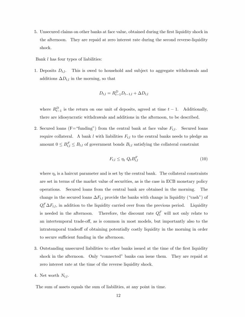
5. Unsecured claims on other banks at face value, obtained during the first liquidity shock in

the afternoon. They are repaid at zero interest rate during the second reverse-liquidity

shock.

Bank l has four types of liabilities:

1. Deposits Dt,l. This is owed to household and subject to aggregate withdrawals and

additions ∆Dt,l in the morning, so that

Dt,l = RDt−1Dt−1,l + ∆Dt,l

where RDt−1 is the return on one unit of deposits, agreed at time t − 1. Additionally,

there are idiosyncratic withdrawals and additions in the afternoon, to be described.

2. Secured loans (F=“funding”) from the central bank at face value Ft,l. Secured loans

require collateral. A bank l with liabilities Ft,l to the central banks needs to pledge an

amount 0 ≤ BFt,l ≤ Bt,l of government bonds Bt,l satisfying the collateral constraint

Ft,l ≤ ηt QtBFt,l (10)

where ηt is a haircut parameter and is set by the central bank. The collateral constraints

are set in terms of the market value of securities, as is the case in ECB monetary policy

operations. Secured loans from the central bank are obtained in the morning. The

change in the secured loans ∆Ft,l provide the banks with change in liquidity (“cash”) of

QFt ∆Ft,l, in addition to the liquidity carried over from the previous period. Liquidity

is needed in the afternoon. Therefore, the discount rate QFt will not only relate to

an intertemporal trade-off, as is common in most models, but importantly also to the

intratemporal tradeoff of obtaining potentially costly liquidity in the morning in order

to secure suffi cient funding in the afternoon.

3. Outstanding unsecured liabilities to other banks issued at the time of the first liquidity

shock in the afternoon. Only “connected”banks can issue them. They are repaid at

zero interest rate at the time of the reverse liquidity shock.

4. Net worth Nt,l.

The sum of assets equals the sum of liabilities, at any point in time.

12

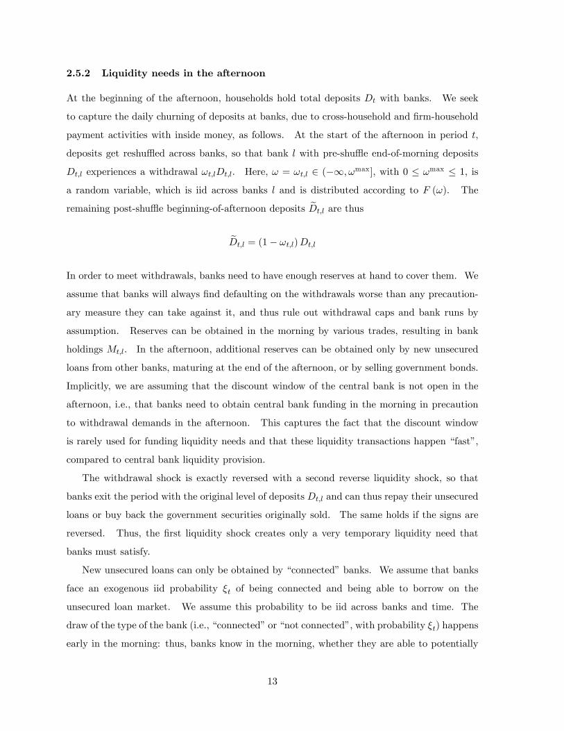
2.5.2 Liquidity needs in the afternoon

At the beginning of the afternoon, households hold total deposits Dt with banks. We seek

to capture the daily churning of deposits at banks, due to cross-household and firm-household

payment activities with inside money, as follows. At the start of the afternoon in period t,

deposits get reshuffl ed across banks, so that bank l with pre-shuffl e end-of-morning deposits

Dt,l experiences a withdrawal ωt,lDt,l. Here, ω = ωt,l ∈ (−∞, ωmax], with 0 ≤ ωmax ≤ 1, is

a random variable, which is iid across banks l and is distributed according to F (ω). The

remaining post-shuffl e beginning-of-afternoon deposits Dt,l are thus

Dt,l = (1− ωt,l)Dt,l

In order to meet withdrawals, banks need to have enough reserves at hand to cover them. We

assume that banks will always find defaulting on the withdrawals worse than any precaution-

ary measure they can take against it, and thus rule out withdrawal caps and bank runs by

assumption. Reserves can be obtained in the morning by various trades, resulting in bank

holdings Mt,l. In the afternoon, additional reserves can be obtained only by new unsecured

loans from other banks, maturing at the end of the afternoon, or by selling government bonds.

Implicitly, we are assuming that the discount window of the central bank is not open in the

afternoon, i.e., that banks need to obtain central bank funding in the morning in precaution

to withdrawal demands in the afternoon. This captures the fact that the discount window

is rarely used for funding liquidity needs and that these liquidity transactions happen “fast”,

compared to central bank liquidity provision.

The withdrawal shock is exactly reversed with a second reverse liquidity shock, so that

banks exit the period with the original level of deposits Dt,l and can thus repay their unsecured

loans or buy back the government securities originally sold. The same holds if the signs are

reversed. Thus, the first liquidity shock creates only a very temporary liquidity need that

banks must satisfy.

New unsecured loans can only be obtained by “connected”banks. We assume that banks

face an exogenous iid probability ξt of being connected and being able to borrow on the

unsecured loan market. We assume this probability to be iid across banks and time. The

draw of the type of the bank (i.e., “connected”or “not connected”, with probability ξt) happens

early in the morning: thus, banks know in the morning, whether they are able to potentially

13

borrow in the afternoon or whether they need to potentially sell government bonds instead.

Every bank can lend unsecured, if they so choose.

If banks do not have access to the unsecured loan market, they will need to sell government

bonds, in case of liquidity needs. They can only do so with the portion that has not yet been

pledged to the central bank. With ωmax as the maximal withdrawal shock, non-connected

banks therefore have to hold government securities satisfying

ωmaxDt,l −Mt,l ≤ ηtQt(Bt,l −BF

t,l

)(11)

where 0 ≤ ηt ≤ 1 is a haircut parameters imposed by other lending banks, if we interpret

this sale of government bonds as a private repo or private secured borrowing, and where the

constraint is in terms of the unpledged portion of the government bond holdings Bt,l −BFt,l.

As all the afternoon transactions are reversed at the end of the afternoon and since all

within-afternoon interest rates are zero, banks will be entirely indifferent between using any

of the available sources of liquidity: what happens in the afternoon stays in the afternoon.

The only impact of these choices and restrictions is that banks need to plan ahead of time

in the morning to make sure that they have enough funding in the afternoon, in the worst

case scenario. If a bank is unconnected, that worse-case scenario is particularly bad, as it

needs to have enough of cash reserves plus unpledged bonds to meet the maximally conceivable

afternoon deposit withdrawal.

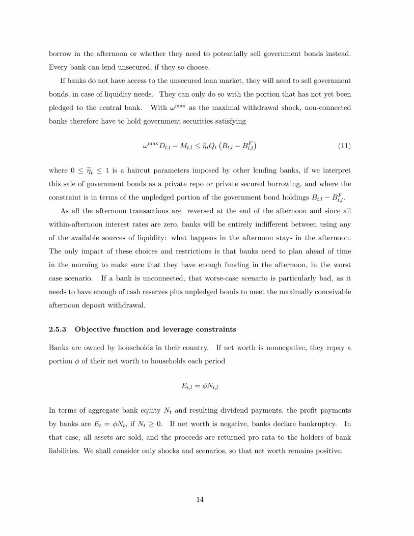
2.5.3 Objective function and leverage constraints

Banks are owned by households in their country. If net worth is nonnegative, they repay a

portion φ of their net worth to households each period

Et,l = φNt,l

In terms of aggregate bank equity Nt and resulting dividend payments, the profit payments

by banks are Et = φNt, if Nt ≥ 0. If net worth is negative, banks declare bankruptcy. In

that case, all assets are sold, and the proceeds are returned pro rata to the holders of bank

liabilities. We shall consider only shocks and scenarios, so that net worth remains positive.

14

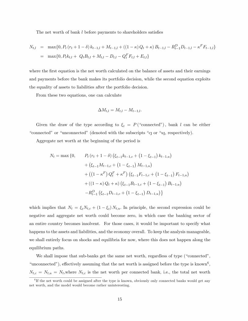
The net worth of bank l before payments to shareholders satisfies

Nt,l = max{0, Pt (rt + 1− δ) kt−1,l +Mt−1,l + ((1− κ)Qt + κ)Bt−1,l −RDt−1Dt−1,l − κFFt−1,l}

= max{0, Ptkt,l + QtBt,l +Mt,l −Dt,l −QFt Ft,l + Et,l}

where the first equation is the net worth calculated on the balance of assets and their earnings

and payments before the bank makes its portfolio decision, while the second equation exploits

the equality of assets to liabilities after the portfolio decision.

From these two equations, one can calculate

∆Mt,l = Mt,l −Mt−1,l.

Given the draw of the type according to ξt = P (“connected”) , bank l can be either

“connected”or “unconnected”(denoted with the subscripts “c or “u, respectively).

Aggregate net worth at the beginning of the period is

Nt = max {0, Pt (rt + 1− δ)(ξt−1kt−1,c +

(1− ξt−1

)kt−1,u

)+(ξt−1Mt−1,c +

(1− ξt−1

)Mt−1,u

)+((

1− κF)QFt + κF

) (ξt−1Ft−1,c +

(1− ξt−1

)Ft−1,u

)+ ((1− κ)Qt + κ)

(ξt−1Bt−1,c +

(1− ξt−1

)Bt−1,u

)−RDt−1

(ξt−1Dt−1,c +

(1− ξt−1

)Dt−1,u

)}which implies that Nt = ξtNt,c + (1− ξt)Nt,u. In principle, the second expression could be

negative and aggregate net worth could become zero, in which case the banking sector of

an entire country becomes insolvent. For those cases, it would be important to specify what

happens to the assets and liabilities, and the economy overall. To keep the analysis manageable,

we shall entirely focus on shocks and equilibria for now, where this does not happen along the

equilibrium paths.

We shall impose that sub-banks get the same net worth, regardless of type (“connected”,

“unconnected”), effectively assuming that the net worth is assigned before the type is known6,

Nt,c = Nt,u = Nt,where Nt,c is the net worth per connected bank, i.e., the total net worth

6 If the net worth could be assigned after the type is known, obviously only connected banks would get anynet worth, and the model would become rather uninteresting.

15

in all connected banks is ξtNt,c, the total net worth in all unconnected banks is (1− ξt)Nt,u.

Correspondingly, all assets and liabilities are likewise distributed equally, regardless of type

(again, assuming that this redistribution is done before the new type is drawn for each sub-

bank).

Summing this and imposing the two previous equations shows that total net worth is Nt,

as it should be. Therefore, we shall drop the distinction between Nt,c, Nt,u and Nt. The

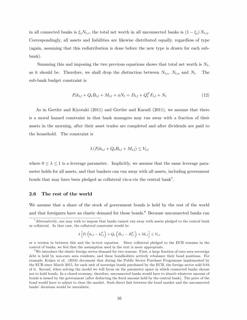
sub-bank budget constraint is

Ptkt,l +QtBt,l +Mt,l + φNt = Dt,l +QFt Ft,l +Nt (12)

As in Gertler and Kiyotaki (2011) and Gertler and Karadi (2011), we assume that there

is a moral hazard constraint in that bank managers may run away with a fraction of their

assets in the morning, after their asset trades are completed and after dividends are paid to

the household. The constraint is

λ (Ptkt,l +QtBt,l +Mt,l) ≤ Vt,l

where 0 ≤ λ ≤ 1 is a leverage parameter. Implicitly, we assume that the same leverage para-

meter holds for all assets, and that bankers can run away with all assets, including government

bonds that may have been pledged as collateral vis-a-vis the central bank7.

2.6 The rest of the world

We assume that a share of the stock of government bonds is held by the rest of the world

and that foreigners have an elastic demand for those bonds.8 Because unconnected banks can

7Alternatively, one may wish to impose that banks cannot run away with assets pledged to the central bankas collateral. In that case, the collateral constraint would be

λ[Pt(kt,l − kFt,l

)+Qt

(Bt,l −BFt,l

)+Mt,l

]≤ Vt,l

or a version in between this and the in-text equation. Since collateral pledged to the ECB remains in thecontrol of banks, we feel that the assumption used in the text is more appropriate.

8We introduce the elastic foreign sector demand for two reasons. First, a large fraction of euro area sovereigndebt is held by non-euro area residents, and these bondholders actively rebalance their bond positions. Forexample, Koijen et al. (2016) document that during the Public Sector Purchase Programme implemented bythe ECB since March 2015, for each unit of sovereign bonds purchased by the ECB, the foreign sector sold 0.64of it. Second, when solving the model we will focus on the parameter space in which connected banks choosenot to hold bonds. In a closed economy, therefore, unconnected banks would have to absorb whatever amount ofbonds is issued by the government (after deducting the fixed amount held by the central bank). The price of thebond would have to adjust to clear the market. Such direct link between the bond market and the unconnectedbanks’decisions would be unrealistic.

16

buy or sell bonds to foreigners, they can change their bond holdings independently from the

government’s outstanding stock of debt.

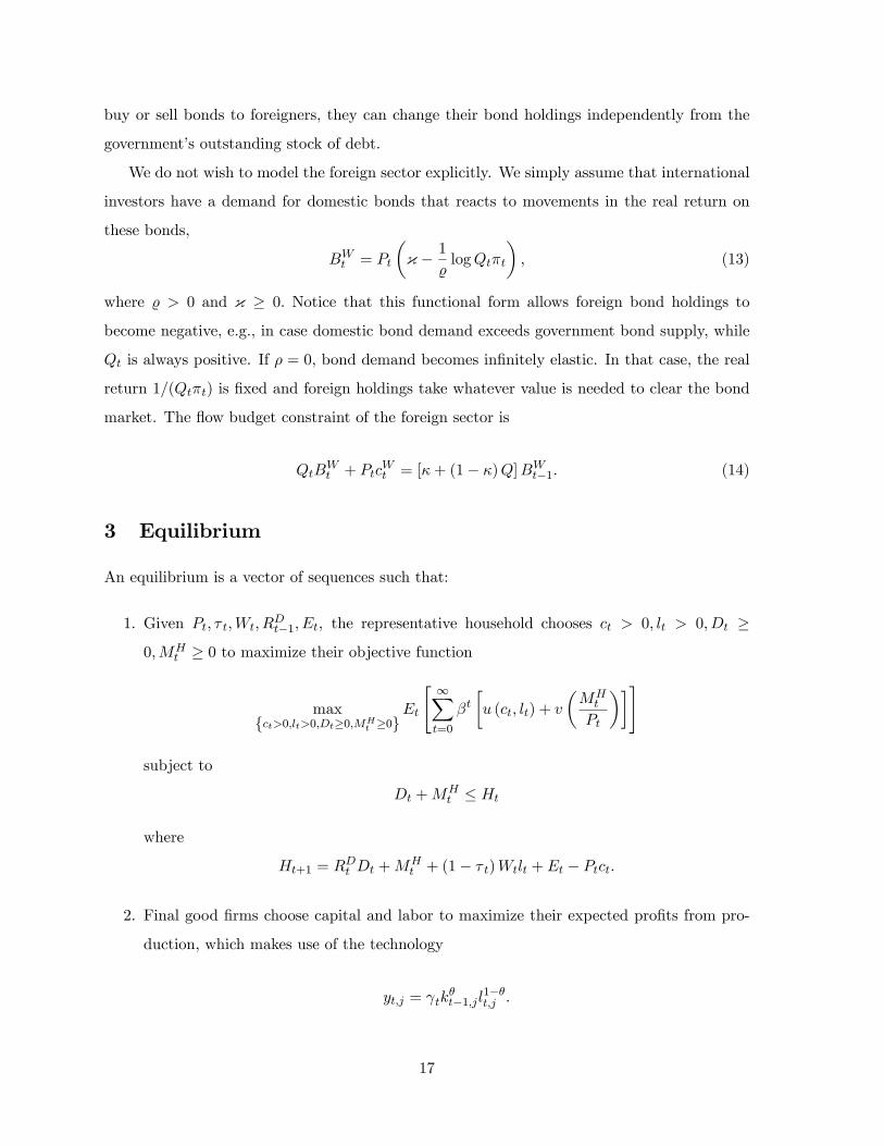
We do not wish to model the foreign sector explicitly. We simply assume that international

investors have a demand for domestic bonds that reacts to movements in the real return on

these bonds,

BWt = Pt

(κ − 1

%logQtπt

), (13)

where % > 0 and κ ≥ 0. Notice that this functional form allows foreign bond holdings to

become negative, e.g., in case domestic bond demand exceeds government bond supply, while

Qt is always positive. If ρ = 0, bond demand becomes infinitely elastic. In that case, the real

return 1/(Qtπt) is fixed and foreign holdings take whatever value is needed to clear the bond

market. The flow budget constraint of the foreign sector is

QtBWt + Ptc

Wt = [κ+ (1− κ)Q]BW

t−1. (14)

3 Equilibrium

An equilibrium is a vector of sequences such that:

1. Given Pt, τ t,Wt, RDt−1, Et, the representative household chooses ct > 0, lt > 0, Dt ≥

0,MHt ≥ 0 to maximize their objective function

max{ct>0,lt>0,Dt≥0,MH

t ≥0}Et

[ ∞∑t=0

βt[u (ct, lt) + v

(MHt

Pt

)]]

subject to

Dt +MHt ≤ Ht

where

Ht+1 = RDt Dt +MHt + (1− τ t)Wtlt + Et − Ptct.

2. Final good firms choose capital and labor to maximize their expected profits from pro-

duction, which makes use of the technology

yt,j = γtkθt−1,jl

1−θt,j .

17

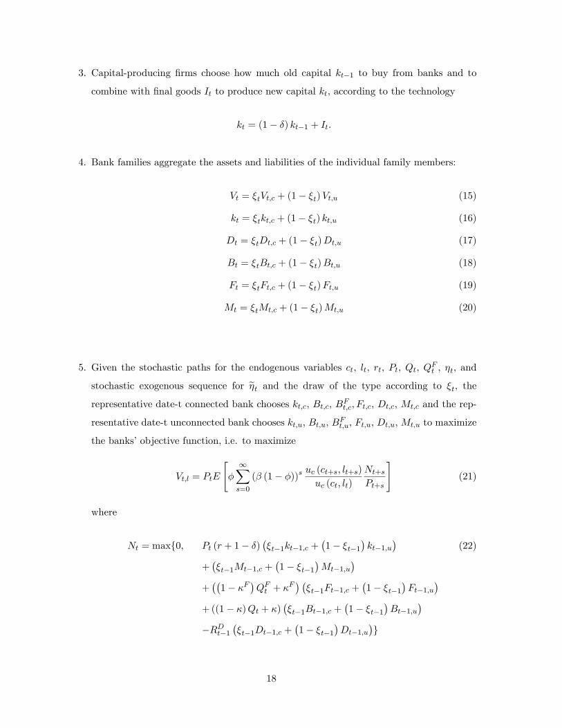
3. Capital-producing firms choose how much old capital kt−1 to buy from banks and to

combine with final goods It to produce new capital kt, according to the technology

kt = (1− δ) kt−1 + It.

4. Bank families aggregate the assets and liabilities of the individual family members:

Vt = ξtVt,c + (1− ξt)Vt,u (15)

kt = ξtkt,c + (1− ξt) kt,u (16)

Dt = ξtDt,c + (1− ξt)Dt,u (17)

Bt = ξtBt,c + (1− ξt)Bt,u (18)

Ft = ξtFt,c + (1− ξt)Ft,u (19)

Mt = ξtMt,c + (1− ξt)Mt,u (20)

5. Given the stochastic paths for the endogenous variables ct, lt, rt, Pt, Qt, QFt , ηt, and

stochastic exogenous sequence for ηt and the draw of the type according to ξt, the

representative date-t connected bank chooses kt,c, Bt,c, BFt,c, Ft,c, Dt,c, Mt,c and the rep-

resentative date-t unconnected bank chooses kt,u, Bt,u, BFt,u, Ft,u, Dt,u, Mt,u to maximize

the banks’objective function, i.e. to maximize

Vt,l = PtE

[φ∞∑s=0

(β (1− φ))suc (ct+s, lt+s)

uc (ct, lt)

Nt+s

Pt+s

](21)

where

Nt = max{0, Pt (r + 1− δ)(ξt−1kt−1,c +

(1− ξt−1

)kt−1,u

)(22)

+(ξt−1Mt−1,c +

(1− ξt−1

)Mt−1,u

)+((

1− κF)QFt + κF

) (ξt−1Ft−1,c +

(1− ξt−1

)Ft−1,u

)+ ((1− κ)Qt + κ)

(ξt−1Bt−1,c +

(1− ξt−1

)Bt−1,u

)−RDt−1

(ξt−1Dt−1,c +

(1− ξt−1

)Dt−1,u

)}

18

s.t. for l = c, u,

Vt,l ≥ λ (Ptkt,l +QtBt,l +Mt,l)

0 ≤ Bt,l −BFt,l

Ptkt,l +QtBt,l +Mt,l + φNt = Dt,l +QFt Ft,l +Nt

Ft,l ≤ ηtQtBFt,l

as well as

ωmaxDt,u −Mt,u ≤ ηtQt(Bt,u −BF

t,u

)for the unconnected banks.

6. The central banks chooses the total amount of money supply M t, the haircut parameter

ηt, the discount factor on central bank funds QFt , the bond purchases B

Ct as well as the

seigniorage payment St. It satisfies the balance sheet constraint

St = QFt F t +QtBCt −M t (23)

and the budget constraint, rewritten as

M t = QFt−1F t−1 + Qt−1BCt−1 +QFt

(F t −

(1− κF

)F t−1

)(24)

−κFF t−1 + Qt(BCt − (1− κ)BC

t−1)− κBC

t−1

7. The government satisfies the debt evolution constraint, the budget constraint and the

tax rule

Bt = (1− κ)Bt−1 + ∆Bt (25)

Pt gt + κBt−1 = τ tWtlt + Qt∆Bt + St (26)

τ t − τ∗ = α(Bt −B

∗), (27)

where τ∗ is the level of the income tax necessary to stabilizes the debt at B∗.

19

8. The foreign sector chooses the amount of domestic bonds to hold

BWt = Pt

(κ − 1

%logQtπt

), (28)

and satisfies the budget constraint

QtBWt + Ptc

Wt = [κ+ (1− κ)Q]BW

t−1. (29)

9. Markets clear:

ct + gt + It + cWt = yt (30)

Bt = Bt + BCt +BW

t (31)

F t = Ft (32)

M t = Mt + MHt (33)

4 Analysis

We characterize the decision of households, firms and banks in turn.

4.1 Households

The household budget constraint at time t writes as

Dt +MHt ≤ RDt−1Dt−1 +MH

t−1 + (1− τ t−1)Wt−1lt−1 + Et−1 − Pt−1ct−1 (34)

Note that the household’s problem is subject to a non-negativity conditions,

MHt ≥ 0, (35)

Note also that ct > 0, lt > 0, and Dt ≥ 0. We do not list these constraints separately for the

following reasons. For ct > 0 and lt > 0, we can assure nonnegativity with appropriate choice

for preferences and per the imposition of Inada conditions. We constrain the analysis a priori

20

to Dt > 0, despite the possibility in principle that it could be zero or negative when allowing

for more generality9.

Let µHHt denote a Lagrange multiplier on the period-t household budget constraint (34),

and µMt,h the multiplier on the constraint (35). The optimality conditions are given by:

−ul (ct, lt)uc (ct, lt)

= (1− τ t)Wt

Pt

vM

(mht

)= uc (ct, lt)

(RDt − 1

)− µMt,h

uc (ct−1, lt−1)

Pt−1= βRDt

[uc (ct, lt)

Pt

]

where µMt,h = PtµMt,h.

4.2 Firms

First-order conditions arising from the problem of the firms are

yt = γtkθt−1l

1−θt ,

Wtlt = (1− θ)Pt yt,

rt,Akt−1,A = θyt,

kt = (1− δ) kt−1 + It.

4.3 Banks

The run-away constraint (assuming it always binds) is

Vt,l = λ (Ptkt,l +QtBt,l +Mt,l) (36)

The value of the mother bank is Vt, which is given by

Vt = ξtVt,c + (1− ξt)Vt,u (37)

9We have not yet fully analyzed this matter for the dynamic evolution of the economy. It may well be thatnet worth of banks temporarily exceeds the funding needed for financing the capital stock, and that thereforedeposits ought to be negative, rather than positive. For now, the attention is on the steady state analysis,however, and on returns to capital exceeding the returns on deposits.

21

Proposition 1 (linearity) The problem of bank l is linear in net worth and

Vt,l = ψtNt,l (38)

for any bank l and some factor ψt. In particular, Vt,l = 0 if Nt,l = 0.

Proof: Since there are no fixed costs, a bank with twice as much net worth can invest twice

as much in the assets. Furthermore, if a portfolio is optimal at some scale for net worth, then

doubling every portion of that portfolio is optimal at twice that net worth. Thus the value of

the bank is twice as large, giving the linearity above.

We need to calculate Vt,l. The proposition above implies

Vt = ψtNt (39)

giving us a valuation of a marginal unit of net worth at the beginning of period t, for a

representative bank.

Suppose, at the end of the period, the representative “mother bank” has various assets,

kt, Bt, and Mt, brought to it by the various sub-banks as they get together again at the end

of the period. The end-of-period value Vt of the “mother bank”then satisfies

Vt = β (1− φ)Et

[uc (ct+1, lt+1)

uc (ct, lt)

PtPt+1

ψt+1Nt+1

]= ψt,k Ptkt + ψt,BBt + ψt,M Mt − ψt,DDt − ψt,FFt (40)

Per inspecting (22) as well (38), we obtain

ψt,k = β (1− φ)Et

[uc (ct+1, lt+1)

uc (ct, lt)ψt+1 (rt+1 + 1− δ)

](41)

ψt,B = β (1− φ)Et

[uc (ct+1, lt+1)

uc (ct, lt)

PtPt+1

ψt+1 ((1− κ)Qt+1 + κ)

](42)

ψt,D = β (1− φ)Et

[uc (ct+1, lt+1)

uc (ct, lt)

PtPt+1

ψt+1 RDt

](43)

ψt,F = β (1− φ)Et

[uc (ct+1, lt+1)

uc (ct, lt)

PtPt+1

ψt+1((

1− κF)QFt+1 + κF

)](44)

ψt,M = β (1− φ)Et

[uc (ct+1, lt+1)

uc (ct, lt)

PtPt+1

ψt+1

](45)

22

For the sub-banker of type l, write

Vt,l = φNt,A + Vt,l (46)

The sub-bankers contribute to Vt per

Vt,l = ψt,kkt,l + ψt,BBt,l + ψt,MMt,l − ψt,DDt,l − ψt,FFt,l (47)

The run-away constraint for bank l can then be rewritten as

φNt,A + Vt,l ≥ λ (Ptkt,l +QtBt,l +Mt,l) (48)

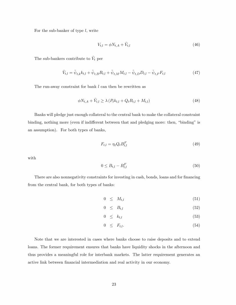
Banks will pledge just enough collateral to the central bank to make the collateral constraint

binding, nothing more (even if indifferent between that and pledging more: then, “binding”is

an assumption). For both types of banks,

Ft,l = ηtQtBFt,l (49)

with

0 ≤ Bt,l −BFt,l (50)

There are also nonnegativity constraints for investing in cash, bonds, loans and for financing

from the central bank, for both types of banks:

0 ≤ Mt,l (51)

0 ≤ Bt,l (52)

0 ≤ kt,l (53)

0 ≤ Ft,l. (54)

Note that we are interested in cases where banks choose to raise deposits and to extend

loans. The former requirement ensures that banks have liquidity shocks in the afternoon and

thus provides a meaningful role for interbank markets. The latter requirement generates an

active link between financial intermediation and real activity in our economy.

23

We can have cases, however, when banks decide not to raise central bank finance, as in

the case of connected banks that can always get afternoon zero-interest rate unsecured loans

from other banks, if the need arises (this is assuming that QFt ≤ 1, otherwise there would be

arbitrage possibilities for banks!). Similarly, banks can decide not to hold cash, if they have

access to afternoon unsecured or secured finance, and if the expected return on capital is higher

than the expected return on money.

To simplify the analysis, we assume (and verify in appendix A) that the economy is in an

interior equilibrium for Dt,l, and kt,l in all the interesting cases we consider. In light of the

considerations above, we explicitly allow for corner solutions for Ft,l, Bt,l and Mt,l.

As for the afternoon, there is no need to keep track of trades, except to make sure that the

afternoon funding constraints for the unconnected banks hold,

ωmaxDt,u −Mt,u ≤ ηtQt(Bt,u −BF

t,u

). (55)

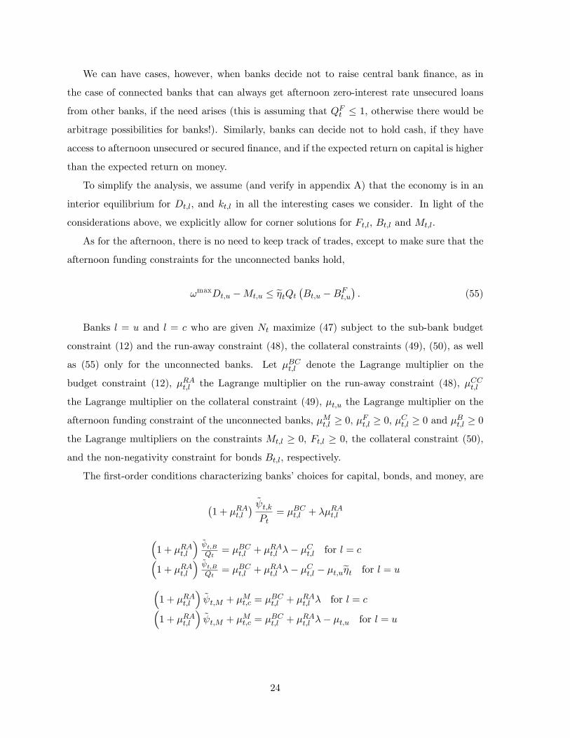
Banks l = u and l = c who are given Nt maximize (47) subject to the sub-bank budget

constraint (12) and the run-away constraint (48), the collateral constraints (49), (50), as well

as (55) only for the unconnected banks. Let µBCt,l denote the Lagrange multiplier on the

budget constraint (12), µRAt,l the Lagrange multiplier on the run-away constraint (48), µCCt,l

the Lagrange multiplier on the collateral constraint (49), µt,u the Lagrange multiplier on the

afternoon funding constraint of the unconnected banks, µMt,l ≥ 0, µFt,l ≥ 0, µCt,l ≥ 0 and µBt,l ≥ 0

the Lagrange multipliers on the constraints Mt,l ≥ 0, Ft,l ≥ 0, the collateral constraint (50),

and the non-negativity constraint for bonds Bt,l, respectively.

The first-order conditions characterizing banks’choices for capital, bonds, and money, are

(1 + µRAt,l

) ψt,kPt

= µBCt,l + λµRAt,l

(1 + µRAt,l

)ψt,BQt

= µBCt,l + µRAt,l λ− µCt,l for l = c(1 + µRAt,l

)ψt,BQt

= µBCt,l + µRAt,l λ− µCt,l − µt,uηt for l = u(1 + µRAt,l

)ψt,M + µMt,c = µBCt,l + µRAt,l λ for l = c(

1 + µRAt,l

)ψt,M + µMt,c = µBCt,l + µRAt,l λ− µt,u for l = u

24

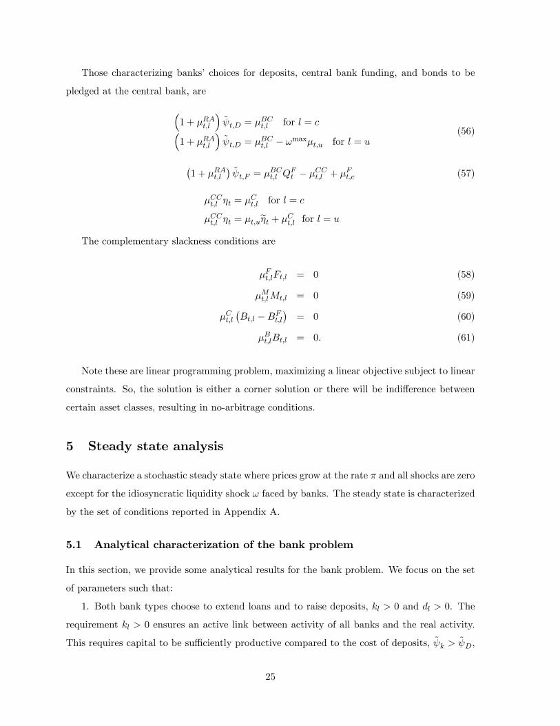
Those characterizing banks’choices for deposits, central bank funding, and bonds to be

pledged at the central bank, are

(1 + µRAt,l

)ψt,D = µBCt,l for l = c(

1 + µRAt,l

)ψt,D = µBCt,l − ωmaxµt,u for l = u

(56)

(1 + µRAt,l

)ψt,F = µBCt,l Q

Ft − µCCt,l + µFt,c (57)

µCCt,l ηt = µCt,l for l = c

µCCt,l ηt = µt,uηt + µCt,l for l = u

The complementary slackness conditions are

µFt,lFt,l = 0 (58)

µMt,lMt,l = 0 (59)

µCt,l(Bt,l −BF

t,l

)= 0 (60)

µBt,lBt,l = 0. (61)

Note these are linear programming problem, maximizing a linear objective subject to linear

constraints. So, the solution is either a corner solution or there will be indifference between

certain asset classes, resulting in no-arbitrage conditions.

5 Steady state analysis

We characterize a stochastic steady state where prices grow at the rate π and all shocks are zero

except for the idiosyncratic liquidity shock ω faced by banks. The steady state is characterized

by the set of conditions reported in Appendix A.

5.1 Analytical characterization of the bank problem

In this section, we provide some analytical results for the bank problem. We focus on the set

of parameters such that:

1. Both bank types choose to extend loans and to raise deposits, kl > 0 and dl > 0. The

requirement kl > 0 ensures an active link between activity of all banks and the real activity.

This requires capital to be suffi ciently productive compared to the cost of deposits, ψk > ψD,

25

which after substituting for ψk and ψD yields:

θy

(ξkc + (1− ξ) ku)+ 1− δ > 1

β. (62)

The requirement that dl > 0 means that both bank types will be subject to liquidity shocks in

the afternoon and thus liquidity management will play an important role for both bank types.

Different bank types may still choose to manage their liquidity differently (through interbank

markets and/or by borrowing from the central bank and saving cash for the afternoon). For

households to deposit with banks we need that RD > 1 or, equivalently,

π

β> 1. (63)

2. The central bank conducts monetary policy by conducting open market operations, i.e.

by changing the amount of bonds bC held on its balance sheet. It also sets the price of central

bank funding, QF , and the haircut η.

3. Connected banks do not borrow from the central bank, µFc > 0 and fc = 0. Note: In

reality, when banks can easily borrow unsecured, they use central bank funding only to manage

their expected liquidity needs, like reserve requirements. Those are set to zero in the model. In

our model, banks will only access central bank funding when their access to interbank markets

is impaired. Indeed, historically, banks have made precautionary use of central bank funding

to satisfy (unexpected) liquidity needs only in crisis periods.

A suffi cient condition for µFc > 0 and fc = 0 is

(1− κF

)QF + κF

QF>π

β= RD. (64)

Note that for κF = 1, this conditions is equivalent to

1

QF>π

β.

The condition is intuitive: if the interest rate on central bank funding is higher than the rate

on deposits, central bank funding will not be used. It is both more expensive in terms of the

interest rate and it requires collateral.

When conditions (62)-(64) hold, we can characterize decisions of connected banks as follows

(the proof is in the Appendix).

26

Proposition 2 (connected banks) Suppose conditions (62)-(64) hold. Then, a connected

bank does not borrow from the central bank. A connected bank does not hold any cash. Moreover,

if the afternoon constraint of unconnected banks binds, µu > 0, then a connected bank does not

hold any bonds, i.e., bc = 0.

Connected banks have access to the unsecured market in which they can smooth out liq-

uidity shocks without a need for collateral. Given condition (64), central bank funding is more

expensive than the cost of deposits so connected banks will not use it for funding purposes.

Similarly, connected banks will not hold any precautionary cash reserves since holding cash

carries an opportunity cost. Whenever the afternoon constraint of unconnected banks binds,

physical return on bonds is lower than the return on capital as bonds command a collateral

premium. However, since connected banks do not need any collateral, they prefer to invest

solely in capital.

Decisions of unconnected banks are as follows (the proof is in the Appendix).

Proposition 3 (unconnected banks) Suppose conditions (62)-(64) hold. If the afternoon

constraint is slack, µu = 0, then an unconnected bank does not borrow from the central bank,

µFu > 0 and fu = 0. Also, if condition

η ≥ ηQFωmax (65)

holds, then an unconnected bank does not borrow from the central bank. If the afternoon

constraint binds and condition

η <ψk −

ψBQ

ψk − ψM(66)

holds, then an unconnected bank does not borrow in the secured market and instead it borrows

only from the central bank and holds money, mu > 0.

If the afternoon constraint is slack, unconnected banks are unconstrained in their afternoon

borrowing in the secured market. Therefore, they do not borrow from the central bank.

Similarly, they do not borrow from the central bank whenever (65) holds, as private haircut η on

bonds is favorable compared to the cost of central bank funding ηQF weighted by the maximum

afternoon withdrawals ωmax. Since ηQF ≤ 1 holds, an even simpler suffi cient condition for (65)

to hold is η ≥ ωmax. By contrast, whenever (66) holds, private haircut η is so unfavorable that

unconnected banks do not use secured market and borrow from the central bank instead. Since

27

unconnected banks borrow from the central bank, their afternoon constraint binds, µu > 0. It

follows that money holdings are positive, mu = ωmaxdu > 0.

6 Numerical analysis

Throughout the numerical analysis, we assume the following functional form for utility: u (ct, lt)+

v(MHtPt

)= log ct + χ log

(MHtPt

)− lt. Notice that we use the log specification also for real bal-

ances, so that the ratio ctmHt

depends on(RDt − 1

), consistent with a transaction technology

specification.

We first describe our calibration strategy. We then use a numerical analysis to illustrate

the properties of our model under specific disruptions of the interbank markets.

6.1 Calibration

In order to evaluate the macroeconomic impact of disruptions in funding markets, we calibrate

the model to capture main features of the euro area economy in normal times.

In the model, each period is a quarter. We set the depreciation rate at δ = 0.02,the capital

income share θ at 0.33 and the discount factor at β = 0.995.10

The fraction of government bonds repaid each period, κ, is 0.11, corresponding to an

average maturity of the outstanding stock of sovereign bonds of 9 years.11 The parameters

determining haircuts on bonds applied by the private market and by the central bank in normal

times are set equal to each other, at η = η = 0.97 (where 1 − η = 1 − η = 0.03 corresponds

to the 3% haircut). The value for the central bank corresponds to the haircut imposed by the

ECB on category 1 securities (fixed coupon bonds with high credit quality) in 2010.12 The

private market haircut value is taken from LCH.Clearnet , a large European-based multi-asset

clearing house, and refers to an average haircut on French, German and Dutch bonds across

all maturities in 2010.10The inverse of the discount factor 1/β determines the real rate on household deposits. This rate has been

very low in the euro area (in fact, it was negative for overnight deposits both before and after the onset of thefinancial crisis). To match this stylized fact, we choose a relatively high discount rate β.11Andrade et al. (2016) compute an average remaining maturity of 9 years for all eligible sovereign bonds

for purchases by the Eurosystem, in the context of the Public Sector Purchase Programme implemented since2015. The data refer to the period from 9 March 2015 to 30 December 2015. Using data from the SecuritiesHolding Statistics for the period 2013Q4-2014Q4, Koijen et al. (2016) compute that eligible sovereign bondswere a large fraction of the total outstanding stock of euro area public debt (around 70%).12The ECB reports a haircut of 3% on this asset category also during the 2004-2009 period. Source: ECB

dataset.

28

Two novel parameters of our model, which capture frictions in the funding markets and are

key to determining banks’choices, are the share of “connected”banks, ξ, and the maximum

fraction of deposits that households can withdraw in the afternoon, ωmax. We compute the

average pre-crisis value of ξ using data from Euro Area Money Market Survey (2013), which

covers a panel of 98 euro area credit institutions.13 We set ξ at 0.42, the average ratio of the

annual cumulative quarterly turnover in the unsecured market segment over the sum of the

annual cumulative turnover in the secured and unsecured segments, over the period 2004-2007

(where 2004 is the first year with an observation in the survey, and 2007 is the last year before

the crisis). When we assess the impact of money market freezes, we also compute the same

average for the crisis period, i.e. over the period 2008-2013 (where 2013 is the last available

observation in the survey). The average value for that period is 0.24.

We compute ωmax using the information embedded in the liquidity coverage ratio (LCR)

- a prudential instrument that requires banks to hold high-quality liquid assets (HQLA) in

an amount that allows banks to meet 30-days liquidity outflows under stress. As we are

interested in maximum outflows, the “stressed”scenario as considered in the LCR appears to

be an appropriate empirical counterpart for ωmax. The data is taken from the report of the

European Banking Authority (December 2013), EBA henceforth. In 2013, the EBA conducted

the first data exercise to assess the LCR impact on the EU banking sector. The report focuses

on data as of the fourth quarter of 2012. The sample contains 357 EU banks from 21 EU

countries, 50 Group 1 banks (large banks, CT1 capital of EUR 3 billion or above), and 307

Group 2 banks (CT1 capital below EUR 3 billion). Their total assets sum to EUR 33000

billion, the aggregate HQLA to EUR 3739 billion and their net monthly cash outflows to EUR

3251 billion. We calculate ωmax as the ratio of the monthly net cash outflows over total assets

so that ωmax = 0.1.14

We choose the parameter of the foreign demand for bonds, κ, to ensure that, if foreign bond

holdings take a value consistent with our target for the share of those holdings in total debt

13The survey provides information on annual cumulative quarterly turnover in the secured and unsecuredmarket segments, as reported at the end of each year’s second quarter. The unsecured segment comprises allunsecured transactions (total maturities and total turnover). The secured market segment is the repo market(and also includes total maturities and turnover).14 In our model, banks hold liquid assets in the amount of ηQ

(Bu −BFu

)+Mu to cover afternoon withdrawals

ωmaxD. Since F = 0 in our calibrated steady state, and net worth is a small fraction of total liabilities, D canbe approximated with total assets. Assuming that the afternoon constraint binds, we can calculate ωmax as theshare of the net monthly cash outflow over total assets.

29

(as discussed below), then Q and π also take the targeted value at that steady state.15 The

steady state calibration cannot inform us about ρ, so we pick a reasonably low value to ensure

an elastic demand function that stabilizes the return on the bond, i.e. we set ρ = 0.09.16 We

check robustness to alternative values (not reported) and find little impact on the quantitative

assessment of money market disruptions.

We are left with six parameters that we calibrate to jointly minimize the squared log-

deviation of some model-based predictions on key variables from their empirical counterparts:

the share of net worth distributed by banks as dividends, φ, the share of assets bankers can run

away with, λ, the coeffi cient determining the utility from money holdings for households, χ,

the expenditure on public goods, g, the amount of government bonds purchased by the central

bank, BC , and the targeted stock of debt in the economy, B∗. The targeted variables are: i)

average debt to GDP; ii) bank leverage ; iii) lending spread; iv) share of banks’bond holdings

in total debt; v) share of foreign sector’s bond holdings in total debt; and vi) average inflation.

Table 2 summarizes all parameter values.

Table 3 reports the value taken by the six targets in the data (computed over the pre-crisis

period, 1999-2006, unless otherwise indicated) and the model prediction under the chosen

parameterization.17

6.2 Comparative statics

We assess the macroeconomic impact of disruptions in money markets by means of a compara-

tive statics analysis. We analyze three alternative scenarios: 1) reduced access to the unsecured

money market; 2) increased haircuts in the secured market, and 3) increased probability of

deposit withdrawals.

15For Q, the target is 0.989, corresponding to an average yield on 10-year German government bonds of 4.5percent, over the period 1999-2006. For π, the target is 2 percent annual, corresponding to the observed averageHICP inflation in the euro area over the same period.16A high eleasticity of the foreign demand for bonds is supported by the evidence provided in Koijen et

al. (2016). The authors document the change in foreign holdings of euro area sovereign bonds during thePublic Sector Purchase Programme implemented by the ECB in March 2015. They find that the foreign sectordecreased its holdings by 5.4% during the period 2015Q2-2015Q4, relative to the average holdings during theperiod 2013Q4-2014Q4. Over the same period, the average yield on euro area sovereign bonds declined by 63bps, indicating a high elasticity of the foreign demand to the nominal bond return.17Both the value of leverage and the average lending spread for the euro area are taken from Andrade et al.

(2016). The share of banks’and of foreign sector’s bond holdings in total debt is computed using data for 2015reported in Koijen et al. (2016).

30

6.2.1 Disruptions on the unsecured interbank market

The first exercise we conduct aims at analyzing the macroeconomic effects of the drying up of

the euro area unsecured money markets during the initial phase of the financial crisis.

Figure 4 shows the results of a comparative statics exercise in which the share of connected

banks (i.e., those with access to the unsecured market), ξ, decreases from 0.5 to 0.1. The figure

reports with a solid red line the share of connected banks under our benchmark calibration

(ξ = 0.42), and with a dashed black line the share observed on average during the crisis

(ξ = 0.24).

It is useful to recall the definition of ‘collateral premium’as the difference between the

value to the bank of capital and of bonds, ψk −ψBQ . This difference is positive whenever the

afternoon constraint of the unconnected banks is binding and bonds are held for their collateral

value.

At ξ = 0.5, the collateral premium on bonds is positive but small. The afternoon constraint

for unconnected banks binds. At the same time, the amount of deposits raised by connected

and unconnected banks is of a comparable magnitude. Capital instead is lower for unconnected

banks, as they need to invest part of the funds in bonds to be pledged in the secured market in

the afternoon. Due to the return on bonds being higher than the return on money, unconnected

banks choose not to hold cash for the afternoon. As shown analytically, connected banks hold

neither bonds, nor money, i.e. bc = mc = 0. Those banks combine deposits and net worth to

finance the maximum possible amount of productive capital, kc.

As the share of connected banks decreases (moving leftward in the figure), a larger number

of banks now needs to satisfy possible afternoon liquidity withdrawals by holding bonds and/or

money. Recall that the stock of bonds accepted as collateral in the secured market is in given

supply, b, and held by three types of agents: the central bank (in fixed amounts), the foreign

sector, and the unconnected banks. When the share of unconnected banks rises, so does the

aggregate demand for bonds by the domestic banking sector. The bond price (discount factor)

increases, as does the collateral premium. The afternoon constraint becomes progressively

more binding for unconnected banks. As the nominal (and real) return on the bond falls,

foreign investors are induced to sell some of their holdings of domestic bonds. When ξ falls

below 0.42, the afternoon constraint is so binding that unconnected banks start holding money

in order to relax it. This decreases the demand for bonds by unconnected banks and the price

of bonds declines gradually. At the same time, as unconnected banks start holding money,

31

households decrease their money holdings, which is facilitated by an increase in inflation. This

leads to a decrease in the real return on bonds and a gradual decrease of bond holdings by

the foreign sector. The decrease is not enough, however, to free up a suffi cient amount of

bonds for unconnected banks to be able to raise the same amount of deposits. Therefore, as ξ

falls, the overall effect is that unconnected banks contract deposits and reduce their investment

in capital. Because the share of banks with such behavior increases, the aggregate deposits,

capital and output fall.

Notice that unconnected banks choose not to fund themselves at the central bank. The

private secured market provides a better alternative. In our benchmark calibration, the haircut

applied by the private market and the central bank are identical. At the same time, the private

market is active within the period and therefore funding in that market imposes a gross interest

of one. The central bank, instead, provides funding whose repayment becomes due the following

period and charges a higher interest rate.

In the benchmark calibration with ωmax = 0.1, the contraction in real activity induced

purely by disruptions in the unsecured market is moderate. A fall in the share of connected

banks from ξ = 0.42 (pre-crisis average share of unsecured transactions in total) to ξ = 0.24

(post-crisis average) generates a decline in real activity of around 0.4 percent. The reason is that

planning for moderate liquidity outflows in the afternoon does not constrain the unconnected

banks too much: The amount of resources diverted from investment in capital to the investment

in unproductive assets (bonds) is limited.

The impact of the disruptions in the unsecured market changes substantially if expected

liquidity outflows in the afternoon increase (i.e., if unsecured market disruptions go hand in

hand with possibly higher customer withdrawals). We conduct the same comparative statics

exercise in which we raise ωmax from 0.1 to 0.2 (not reported). The results are qualitatively

similar. However, the contraction of real activity when ξ is reduced from 0.42 to 0.24 is now

4 percent. This higher contraction is driven by a much larger distortion in the allocation of

savings, whereby funds are diverted away from productive capital into unproductive assets.

6.2.2 Disruptions on the secured interbank market

We analyse the impact of disruptions on the secured market by changing the parameter that

determines the collateral haircut in the private market, η (where 1− η is the haircut). Figure

32

5 shows the results of a comparative statics exercise in which η moves from the benchmark

pre-crisis value of 0.97 (denoted with a red solid line) to 0.3.

In our calibrated steady state (the red line where η = 0.97), the collateral premium is posi-

tive and the afternoon constraint binds for unconnected banks. As η falls from 0.97 to 0.8 (the

private haircut increases), unconnected banks need to pledge higher amounts of bonds to satisfy

the afternoon constraint, for the same level of deposits. The value of bonds for unconnected

banks falls. Therefore, they reduce their bond holdings and satisfy the afternoon constraint by

increasing the amount of cash brought into the afternoon, and by slightly decreasing deposits

they take. The bond price falls, increasing the nominal return to holding bonds. Inflation rises

in order to induce households to hold less money, ensuring clearing of the money market. The

overall effect is an increase in the real return on bonds, which induces foreigners to increase

their holdings. Overall, in this region, unconnected banks reduce somewhat their investment

in capital. Connected banks also slightly reduce their investment in capital because the supply

of households’deposits decreases.

When η falls below 0.8, it becomes attractive for the unconnected banks to use central

banking funding. Although the interest rate cost of central bank funding is higher than the

interest rate cost of secured market funding, the central bank haircuts are more favourable

relative to those imposed in the private market. Unconnected banks gradually reduce the share

of bonds pledged in the private market and increase the share pledged at the central bank.

The transition is fast. When η is 0.75, unconnected banks pledge their entire stock of bonds at

the central bank. The availability of central bank funding helps to stabilize the economy. As

neither the haircut nor the interest charged by the central bank changes, unconnected banks

are able to stabilize the amount of deposits they raise and thus their investment in capital.

Overall, a decrease of η from 0.97 to the point where unconnected banks use only central

bank funding (η = 0.75), generates an output contraction of 0.3 percent. If we run the same

comparative statics exercise with ωmax = 0.2, the impact on output increases to 0.8 percent.

The reason for the contained macroeconomic impact is that the availability of central bank

funding put a floor on the decline in deposits and capital. The impact would be more severe

in the absence of the central bank.

33

6.2.3 Increased risk of a depositor run

During the sovereign debt crisis, some euro area countries faced an increased risk of runs

on deposits.18 We explore the macroeconomic impact of this type of market disruption by

increasing the maximum level of expected deposit withdrawals, ωmax, from 0.1 (the value

under our benchmark calibration) to 0.6.

At ωmax = 0.1, the economy is in the calibrated steady state described above. As the

expected deposit withdrawals, ωmax, increase, unconnected banks become more constrained in

the afternoon and the collateral premium - the wedge between the return on capital and the

return on bonds - rises sharply for ωmax below 0.18. Unconnected banks are forced to hold more

bonds and cash to satisfy their afternoon constraint. As unconnected banks demand more cash,

households reduce their money holdings, which is facilitated by a rise in inflation. For values

of ωmax below 0.18, unconnected banks moderately reduce deposits and capital. For values of

ωmax above 0.18, the run-away constraint, given by (36), becomes slack for unconnected banks.

Their deposits start declining, reaching zero when ωmax = 0.6. Because unconnected banks

stop raising deposits, connected banks need to hold whatever is supplied by the households.

To induce households to rebalance their wealth away from deposits and into cash holdings,

inflation declines for ωmax values above 0.18.

The reduction in the aggregate amount of deposits severely limits productive investment

and reduces the capital stock. A doubling of the expected deposit withdrawals compared to

the calibrated steady state value, i.e. an increase in ωmax from 0.1 to 0.2, generates output

losses of around 3 percent.

7 Conclusions

We presented a general equilibrium model where banks can finance their liquidity needs in the

unsecured or secured interbank markets, and where they have also access to collateralized cen-

tral bank funding. The model accounts for the reduced ability of banks to access the unsecured

market during the financial and sovereign crisis, and their shift to secured market funding. It

also accounts for the impaired functioning of the secured market during the sovereign crisis

18For instance, the Wall Street Journal reported that on May 15, 2012, at the peak of the sovereign crisis,Greek depositors withdrew 700 million euros (amounting to 0.4 percent of total deposits) from the country’sbanks on a single day, fueling fears of a bank run.

34

and the increased reliance on central bank liquidity provision, particularly for banks located

in countries with a vulnerable sovereign.

Results from our calibrated model show that disruptions of different segments of the money

markets transmit differently to the macroeconomy. In all cases, the macroeconomic impact

can be sizeable.

Our model can be used to assess the impact of a range of unconventional monetary policy

measures that were undertaken in the euro area since 2008, namely standard interest rate

policy, collateral policy (changes in the composition of the collateral pool or in the haircuts

applied to specific classes of assets), main refinancing operations (including changes in their

maturity), targeted long-term refinancing operations, and asset purchases. We leave this for

future work.

References

[1] Afonso, G. and R. Lagos (2015). “Trade Dynamics in the Market for Federal Funds,”

Econometrica, 83(1), 263—313.

[2] Allen, F. and E. Carletti (2008). “The Role of Liquidity in Financial Crises,” Jackson

Hole Symposium on Maintaining Stability in a Changing Financial System, August 21-23,

2008.

[3] Andrade, P., Breckenfelder, J., De Fiore, F., Karadi, P., and O. Tristani (2016). “The Role

of Liquidity in Financial Crises,”ECB Working Paper Series Nr 1956, European Central

Bank.

[4] Atkeson, A., A. Eisfeldt, and P.-O.Weill (2015). “Entry and Exit in OTC Derivatives

Markets,”Econometrica 83(6), 2231—2292.

[5] Bianchi, J. and S. Bigio (2014). “Banks, Liquidity Management, and Monetary Policy,”

Federal Reserve Bank of Minneapolis Research Department Staff Report 503.

[6] Bhattacharya, S. and D. Gale (1987). “Preference Shocks, Liquidity, and Central Bank

Policy”in W. Barnett and K. Singleton (eds.) New Approaches to Monetary Economics,

Cambridge University Press, Cambridge.

[7] Bocola, L. (2016). “The Pass-Through of Sovereign Risk,”Journal of Political Economy

124 (4), 879—926.

35

[8] Bruche, M. and J. Suarez (2010). “Deposit insurance and money market freezes,”Journal

of Monetary Economics 57, Issue 1, 45—61.

[9] Brunnermeier, M. (2009). “Deciphering the 2007—08 liquidity and credit crunch,”Journal

of Economic Perspectives 23, 77—100.

[10] Drechsler, I., T. Drechsel, D. Marques and P. Schnabl (2016). “Who Borrows From the

Lender of Last Resort?”, Journal of Finance 71(5), 1933—1974.

[11] European Banking Authority (2013). “Report on impact assessment

for liquidity measures under Article 509(1) of the CRR,” available at

https://www.eba.europa.eu/documents/10180/16145/EBA+BS+2013+415

+Report+regarding+LCR+impact.pdf.

[12] European Central Bank (2012). Changes in bank financing patterns.

[13] European Central Bank (2013). Euro money market survey.

[14] Flannery, M. (1996). “Financial Crises, Payment System Problems, and Discount Window

Lending,”Journal of Money Credit and Banking 28, 804—824.

[15] Freixas, X. and C. Holthausen (2005). “Interbank Market Integration under Asymmetric

Information,”Review of Financial Studies 18, 459—490.

[16] Freixas, X. and J. Jorge (2008). “The Role of Interbank Markets in Monetary Policy: A

Model with Rationing,”Journal of Money, Credit and Banking 40, 1151-1176.

[17] Freixas, X., A. Martin, and D. Skeie (2011). “Bank Liquidity, Interbank Markets, and

Monetary Policy,”Review of Financial Studies 24, 2656—2692.

[18] Gennaioli, A. Martin, and Rossi (2014). “Sovereign Default, Domestic Banks, and Finan-

cial Institutions,”Journal of Finance 69(2), 819—866.

[19] Gertler, M. and P. Karadi (2011). “A Model of Unconventional Monetary Policy,”Journal

of Monetary Economy 58, 17-34.

[20] Gertler, M. and N. Kiyotaki (2011). “Financial Intermediation and Credit Policy in Busi-

ness Cycle Analysis,”Handbook of Monetary Economics, Vol. 3A.

36

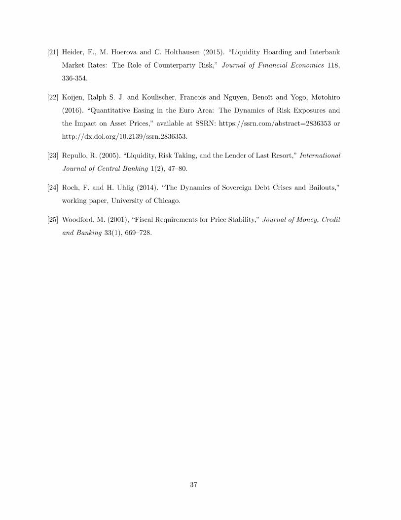
[21] Heider, F., M. Hoerova and C. Holthausen (2015). “Liquidity Hoarding and Interbank

Market Rates: The Role of Counterparty Risk,” Journal of Financial Economics 118,

336-354.

[22] Koijen, Ralph S. J. and Koulischer, Francois and Nguyen, Benoît and Yogo, Motohiro

(2016). “Quantitative Easing in the Euro Area: The Dynamics of Risk Exposures and

the Impact on Asset Prices,” available at SSRN: https://ssrn.com/abstract=2836353 or

http://dx.doi.org/10.2139/ssrn.2836353.

[23] Repullo, R. (2005). “Liquidity, Risk Taking, and the Lender of Last Resort,”International

Journal of Central Banking 1(2), 47—80.

[24] Roch, F. and H. Uhlig (2014). “The Dynamics of Sovereign Debt Crises and Bailouts,”

working paper, University of Chicago.

[25] Woodford, M. (2001), “Fiscal Requirements for Price Stability,”Journal of Money, Credit

and Banking 33(1), 669—728.

37

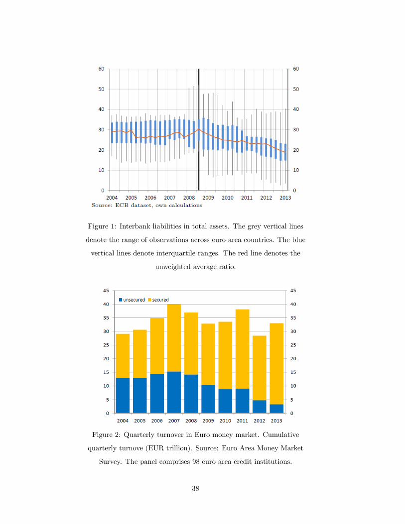
Figure 1: Interbank liabilities in total assets. The grey vertical lines

denote the range of observations across euro area countries. The blue

vertical lines denote interquartile ranges. The red line denotes the

unweighted average ratio.

Figure 2: Quarterly turnover in Euro money market. Cumulative

quarterly turnove (EUR trillion). Source: Euro Area Money Market

Survey. The panel comprises 98 euro area credit institutions.

38

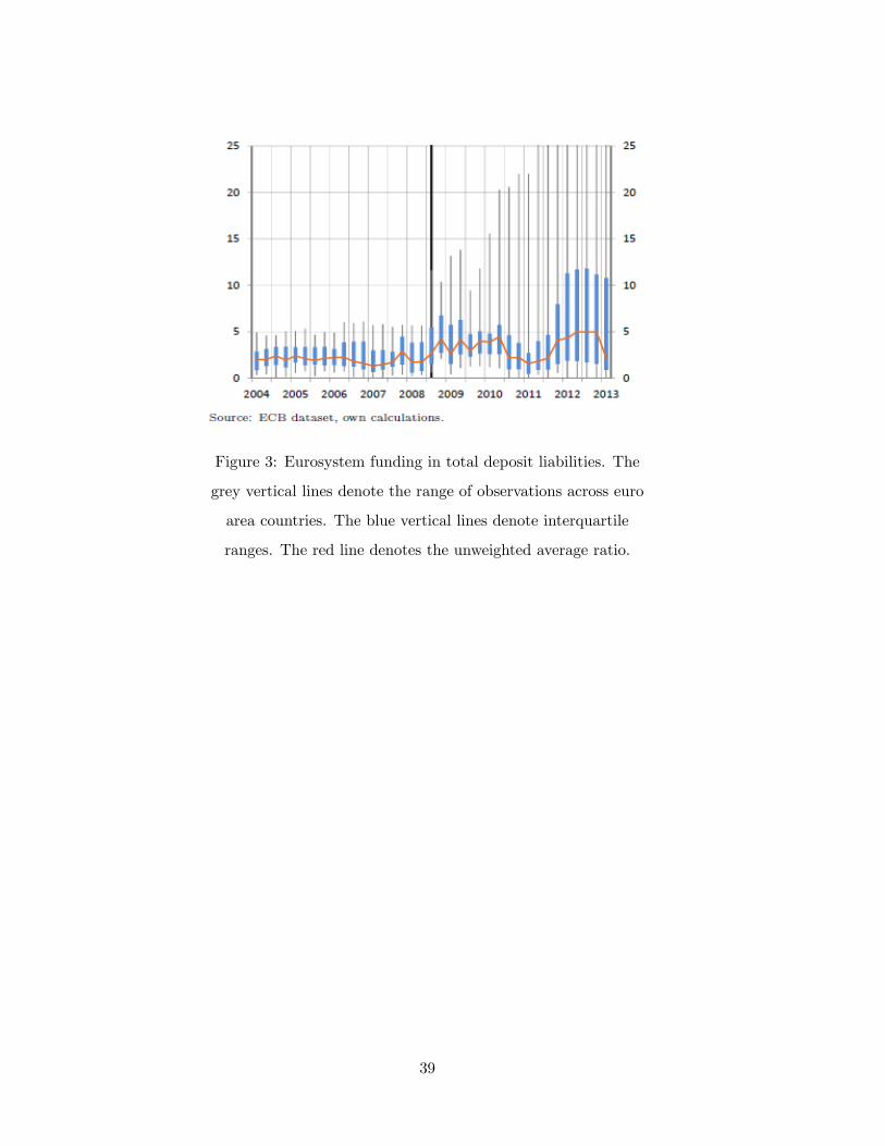
Figure 3: Eurosystem funding in total deposit liabilities. The

grey vertical lines denote the range of observations across euro

area countries. The blue vertical lines denote interquartile

ranges. The red line denotes the unweighted average ratio.

39

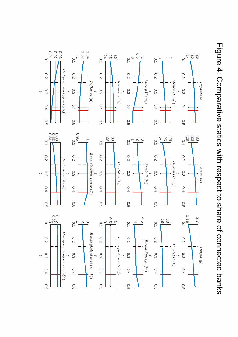
9

0.10.2

0.30.4

0.524 25 26

Deposits

(d)

9

0.10.2

0.30.4

0.526 28 30

Capital(k

)

9

0.10.2

0.30.4

0.52.65

2.7Output(y

)

9

0.10.2

0.30.4

0.50 1 2

MoneyH

(mh)

9

0.10.2

0.30.4

0.524 25 26

Deposits

U(du )

9

0.10.2

0.30.4

0.5

28 30

CapitalU

(ku )

9

0.10.2

0.30.4

0.50

0.5 1MoneyU

(mu )

9

0.10.2

0.30.4

0.51 2 3

BondsU

(bu )

9

0.10.2

0.30.4

0.5

4

4.5BondsForeig

n(bw)

9

0.10.2

0.30.4

0.524 25 26

Deposits

C(dc )

9

0.10.2

0.30.4

0.5

28 30

CapitalC

(kc )

9

0.10.2

0.30.4

0.50

0.5 1BondspledgedCB

(bFu)

9

0.10.2

0.30.4

0.51

1.021.04

Inflation

(:)

9

0.10.2

0.30.4

0.50.95 1

Bonddiscou

ntfactor

(Q)

9

0.10.2

0.30.4

0.51 2 3

Bondspledgedmkt(bu!bFu)

9

0.10.2

0.30.4

0.50.010.020.03

Collprem

ium

(~AK!

~AB=Q

)

9

0.10.2

0.30.4

0.50.810.820.83

Bondretu

rn(

~AB=Q

)

9

0.10.2

0.30.4

0.50

0.010.02

Multip:runaway:con

str:(7RAu

)

Figure 4: Com

parative statics with respect to share of connected banks

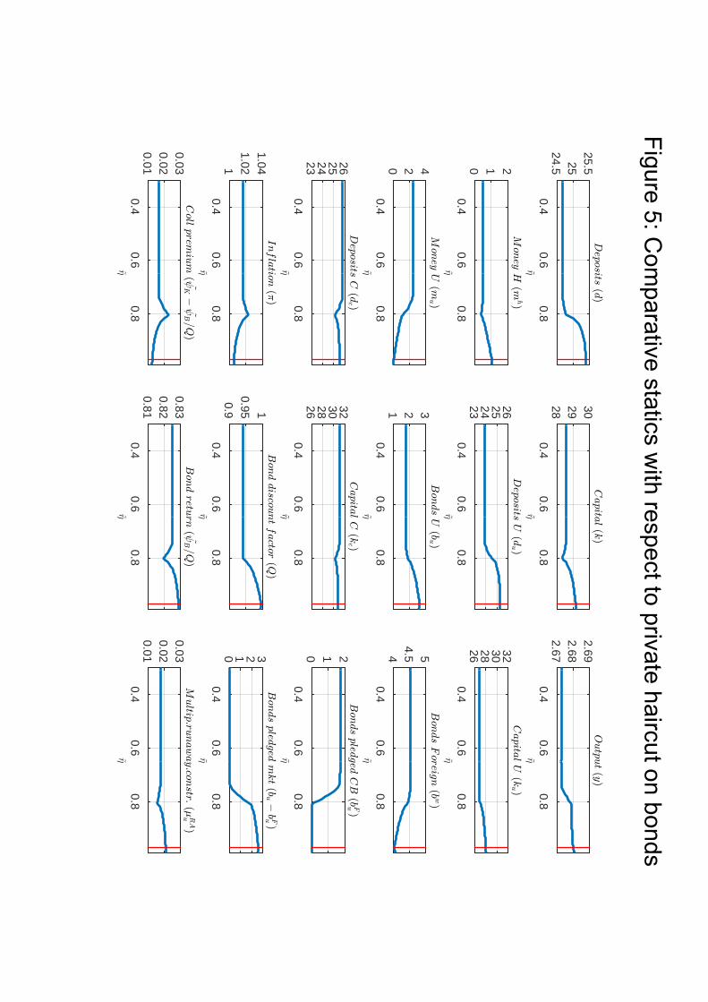
~20.4

0.60.8

24.5 2525.5

Deposits

(d)

~20.4

0.60.8

28 29 30Capital(k

)

~20.4

0.60.8

2.672.682.69

Output(y

)

~20.4

0.60.8

0 1 2MoneyH

(mh)

~20.4

0.60.8

23 24 25 26Deposits

U(du )

~20.4

0.60.8

26 28 30 32CapitalU

(ku )

~20.4

0.60.8

0 2 4MoneyU

(mu )

~20.4

0.60.8

1 2 3BondsU

(bu )

~20.4

0.60.8

44.5 5

BondsForeig

n(bw)

~20.4

0.60.8

23 24 25 26Deposits

C(dc )

~20.4

0.60.8

26 28 30 32CapitalC

(kc )

~20.4

0.60.8

0 1 2BondspledgedCB

(bFu)

~20.4

0.60.8

11.021.04

Inflation

(:)

~20.4

0.60.8

0.90.95 1

Bonddiscou

ntfactor

(Q)

~20.4

0.60.8

0 1 2 3Bondspledgedmkt(bu!bFu)

~20.4

0.60.8

0.010.020.03

Collprem

ium

(~AK!

~AB=Q

)

~20.4

0.60.8

0.810.820.83

Bondretu

rn(

~AB=Q

)

~20.4

0.60.8

0.010.020.03

Multip:runaway:con

str:(7RAu

)

Figure 5: Com

parative statics with respect to private haircut on bonds

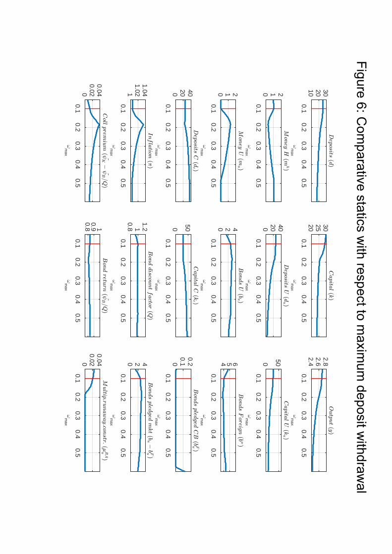
!m

ax

0.10.2

0.30.4

0.510 20 30

Deposits

(d)

!m

ax

0.10.2

0.30.4

0.520 25 30

Capital(k

)

!m

ax

0.10.2

0.30.4

0.52.42.62.8

Output(y

)

!m

ax

0.10.2

0.30.4

0.50 1 2

MoneyH

(mh)

!m

ax

0.10.2

0.30.4

0.50 20 40

Deposits

U(du )

!m

ax

0.10.2

0.30.4

0.50 50

CapitalU

(ku )

!m

ax

0.10.2

0.30.4

0.50 1 2

MoneyU

(mu )

!m

ax

0.10.2

0.30.4

0.50 2 4

BondsU

(bu )

!m

ax

0.10.2

0.30.4

0.5

4 5 6BondsForeig

n(bw)

!m

ax

0.10.2

0.30.4

0.50 20 40

Deposits

C(dc )

!m

ax

0.10.2

0.30.4

0.50 50

CapitalC

(kc )

!m

ax

0.10.2

0.30.4

0.50

0.10.2

BondspledgedCB

(bFu)

!m

ax

0.10.2

0.30.4

0.51

1.021.04

Inflation

(:)

!m

ax

0.10.2

0.30.4

0.50.8 11.2

Bonddiscou

ntfactor

(Q)

!m

ax

0.10.2

0.30.4

0.50 2 4

Bondspledgedmkt(bu!bFu)

!m

ax

0.10.2

0.30.4

0.50

0.020.04

Collprem

ium

(~AK!

~AB=Q

)

!m

ax

0.10.2

0.30.4

0.5

0.80.9 1

Bondretu

rn(

~AB=Q

)

!m

ax

0.10.2

0.30.4

0.50

0.020.04

Multip:runaway:con

str:(7RA

u)

Figure 6: Com

parative statics with respect to m

aximum

deposit withdraw

al

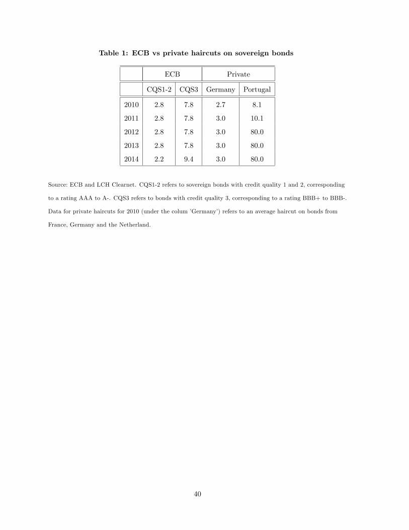
Table 1: ECB vs private haircuts on sovereign bonds

ECB Private

CQS1-2 CQS3 Germany Portugal

2010 2.8 7.8 2.7 8.1

2011 2.8 7.8 3.0 10.1

2012 2.8 7.8 3.0 80.0

2013 2.8 7.8 3.0 80.0

2014 2.2 9.4 3.0 80.0

Source: ECB and LCH Clearnet. CQS1-2 refers to sovereign bonds with credit quality 1 and 2, corresponding

to a rating AAA to A-. CQS3 refers to bonds with credit quality 3, corresponding to a rating BBB+ to BBB-.

Data for private haircuts for 2010 (under the colum ’Germany’) refers to an average haircut on bonds from

France, Germany and the Netherland.

40

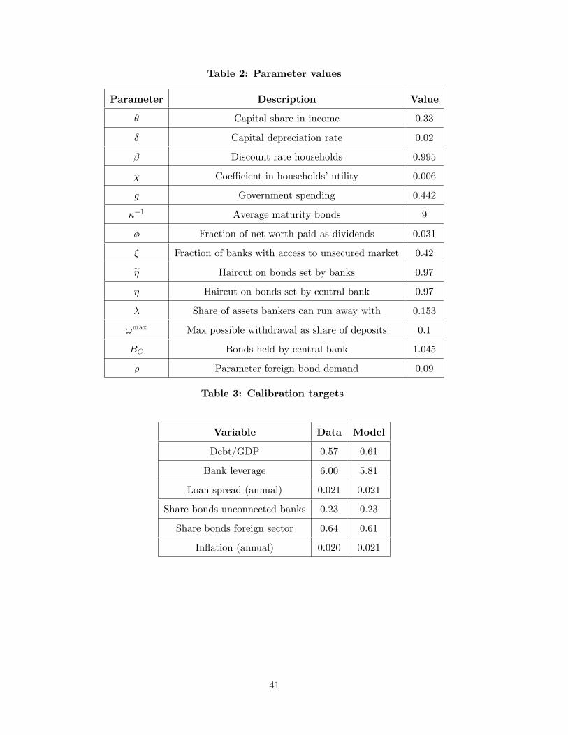
Table 2: Parameter values

Parameter Description Value

θ Capital share in income 0.33

δ Capital depreciation rate 0.02

β Discount rate households 0.995

χ Coeffi cient in households’utility 0.006

g Government spending 0.442

κ−1 Average maturity bonds 9

φ Fraction of net worth paid as dividends 0.031

ξ Fraction of banks with access to unsecured market 0.42

η Haircut on bonds set by banks 0.97

η Haircut on bonds set by central bank 0.97

λ Share of assets bankers can run away with 0.153

ωmax Max possible withdrawal as share of deposits 0.1

BC Bonds held by central bank 1.045

% Parameter foreign bond demand 0.09

Table 3: Calibration targets

Variable Data Model

Debt/GDP 0.57 0.61

Bank leverage 6.00 5.81

Loan spread (annual) 0.021 0.021

Share bonds unconnected banks 0.23 0.23

Share bonds foreign sector 0.64 0.61

Inflation (annual) 0.020 0.021

41

A The equations characterizing the steady state

We characterize the steady state of the model. For simplicity, we focus on the case when capital

is not accepted as collateral at the central bank, ηK = 0. Recall that we already assume that

capital is not accepted as collateral in the private secured market, ηk = 0.

Define a generic variable as the corresponding capital letter variable, divided by the con-

temporaneous price level, i.e. xt = XtPt. The steady state is characterized by the following

conditions:

1. 4 household equations:

RD =π

β

−ul (c, l)uc (c, l)

= (1− τ)w

vM

(mh)

= uc (c, n)(RD − 1

)− µMh

c = (1− τ)wl +

(1

β− 1

)πd+ (1− π)mh + φn

2. 3 firms’equations:

y = γkθl1−θ

wl = (1− θ) y

rk = θy

and

I = δk.

3. 5 central bank equations: 2 equations

s = QF f +QbC −m

m =

[QF − κF 1

π

(1−QF

)]f +

[Q− κ 1

π(1−Q)

]bC

plus the value of 3 variables (policy instruments):

η,QF , bC .

42

Note that the seigniorage revenue of the central bank is given by the interest rate pay-

ments on its assets:

s = κF1

π

(1−QF

)f + κ

1

π(1−Q) bC .

4. 2 government equations:

b = b∗

τ∗ (1− θ) y = g + κ (1−Q)b∗

π−Q

(1− 1

π

)b∗ − s.

where g is exogenous.

5. 4 market clearing equations:

f = f

m = m+mh

b = b+ bC + bH + bW

y = c+ cW + g + I

where the market clearing condition for the goods market (last equation above) is redun-

dant due to the Walras law.

6. 45 (8+18+7+6+6) bank equations:

8 equations common to c and u banks,

ν = ψn

n = max {0, (r + 1− δ) (ξkc + (1− ξ) ku)

+ (ξmc + (1− ξ)mu)1

π

+ ((1− κ)Q+ κ) (ξbc + (1− ξ) bu)1

π

−((

1− κF)QF + κF

)(ξfc + (1− ξ) fu)

1

π

− 1

β(ξdc + (1− ξ) du)

},

43

v = ψkk + ψBb+ ψMm− ψDd− ψF f

ψk = β (1− φ)ψ (r + 1− δ)

ψB = β (1− φ)1

πψ [(1− κ)Q+ κ]

ψD = β (1− φ)1

βψ

ψF = β (1− φ)1

πψ((

1− κF)QF + κF

)ψM = β (1− φ)

1

πψ

9*2=18 equations for l = c, u:

kl +Qbl +ml + φn = dl +QF fl + n

φn+ vl = λ (kl +Qbl +ml)

vl = φn+ vl

vl = ψkkl + ψBbl + ψMml − ψDdl − ψF fl

fl = ηQbFl

µFl fl = 0

µMl ml = 0

µCl(bl − bFl

)= 0

µBl bl = 0

44

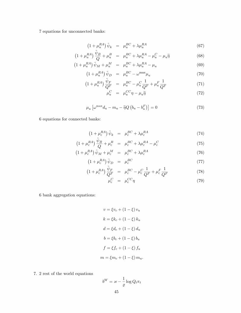
7 equations for unconnected banks:

(1 + µRAu

)ψk = µBCu + λµRAu (67)(

1 + µRAu) ψBQ

+ µBu = µBCu + λµRAu − µCu − µuη (68)(1 + µRAu

)ψM + µMu = µBCu + λµRAu − µu (69)(

1 + µRAu)ψD = µBCu − ωmaxµu (70)(

1 + µRAu) ψFQF

= µBCu − µCu1

QF+ µFu

1

QF(71)

µCu = µCCu η − µuη (72)

µu[ωmaxdu −mu − ηQ

(bu − bFu

)]= 0 (73)

6 equations for connected banks:

(1 + µRAc

)ψk = µBCc + λµRAc (74)(

1 + µRAc) ψBQ

+ µBc = µBCc + λµRAc − µCc (75)(1 + µRAc

)ψM + µMc = µBCc + λµRAc (76)(

1 + µRAc)ψD = µBCc (77)(

1 + µRAc) ψFQF

= µBCc − µCc1

QF+ µFc

1

QF(78)

µCc = µCCc η (79)

6 bank aggregation equations:

v = ξvc + (1− ξ) vu

k = ξkc + (1− ξ) ku

d = ξdc + (1− ξ) du

b = ξbc + (1− ξ) bu

f = ξfc + (1− ξ) fu

m = ξmc + (1− ξ)mu.

7. 2 rest of the world equations

bW = κ − 1

%logQtπt

45

QbW + cW = [κ+ (1− κ)Q]bW

π.

These are 66 equations (one redundant by the Walras law). The endogenous variables are

65: y, k, c, cW , l, d, n,mh, b, bW , f,m, v, v, b, τ∗,

ψ, ψk, ψB, ψM , ψD, ψF , µu, w, r,Q,RD, π, I, s, f ,m

plus {

kl,ml, fl, bl, bFl , dl, vl, vl, µ

Fl , µ

Ml , µ

RAl , µBCl , µCCl , µCl , µ

Bl

},

plus the value of the three policy instruments

ηA, QF , bC ,

and of the following exogenous variables:

g, ξ.

The bank first-order conditions can be further simplified as follows. For the unconnected

banks, conditions (74)-(79) can be simplified to:

µu[ωmaxdu −mu − ηQ

(bu − bFu

)]= 0 (80)

ωmaxµu =(1 + µRAu

) (ψk − ψD

)− λµRAu (81)

µCCu η =(1 + µRAu

)(ψk −

ψBQ

)− µBu (82)

µMu =(1 + µRAu

) (ψk − ψM

)− µu (83)

µFu1

QF=

(1 + µRAu

)( ψFQF− ψD

)− ωmaxµu + µCCu

1

QF(84)

46

For the connected banks, conditions (74)-(79) can be simplified to,

µRAc =ψk − ψD

λ−(ψk − ψD

) (85)

µBc =(1 + µRAc

)(ψk −

ψBQ

)− µCCc η (86)

µMc =(1 + µRAc

) (ψk − ψM

)(87)

µFc1

QF=

(1 + µRAc

)( ψFQF− ψD

)+ µCCc

1

QF(88)

B Proofs

Proof of Proposition 2

By (64), we have µFc > 0 and fc = 0. We first claim that µCc = 0. Intuitively, if a bank

l does not borrow from the central bank, it cannot be collateral-constrained at its borrowing

from the central bank. Consider the following complementary slackness conditions in the bank

problem:

µCl(bl − bFl

)= 0

Since fl = 0, we have that bFl = 0 since fl = ηQbFl and bFl ≥ 0. Therefore, the above

complementary slackness condition simplifies to

µCl bl = 0.

There are two possibilities: either the bond holdings are positive, bl > 0 or they are zero,

bl = 0. In the former case, it follows that µCl = 0, which proves the claim. In the latter case,

we have bl = 0, and a bank does not hold any bonds, does not pledge any bonds, and is not

constrained by the bond collateral constraint, µCl = 0. Therefore, µCl = 0 holds for a bank

that does not borrow from the central bank.

We next show that connected banks do not hold any cash. First-order condition (87) for

connected banks implies that whenever

ψA,k > ψA,M

47

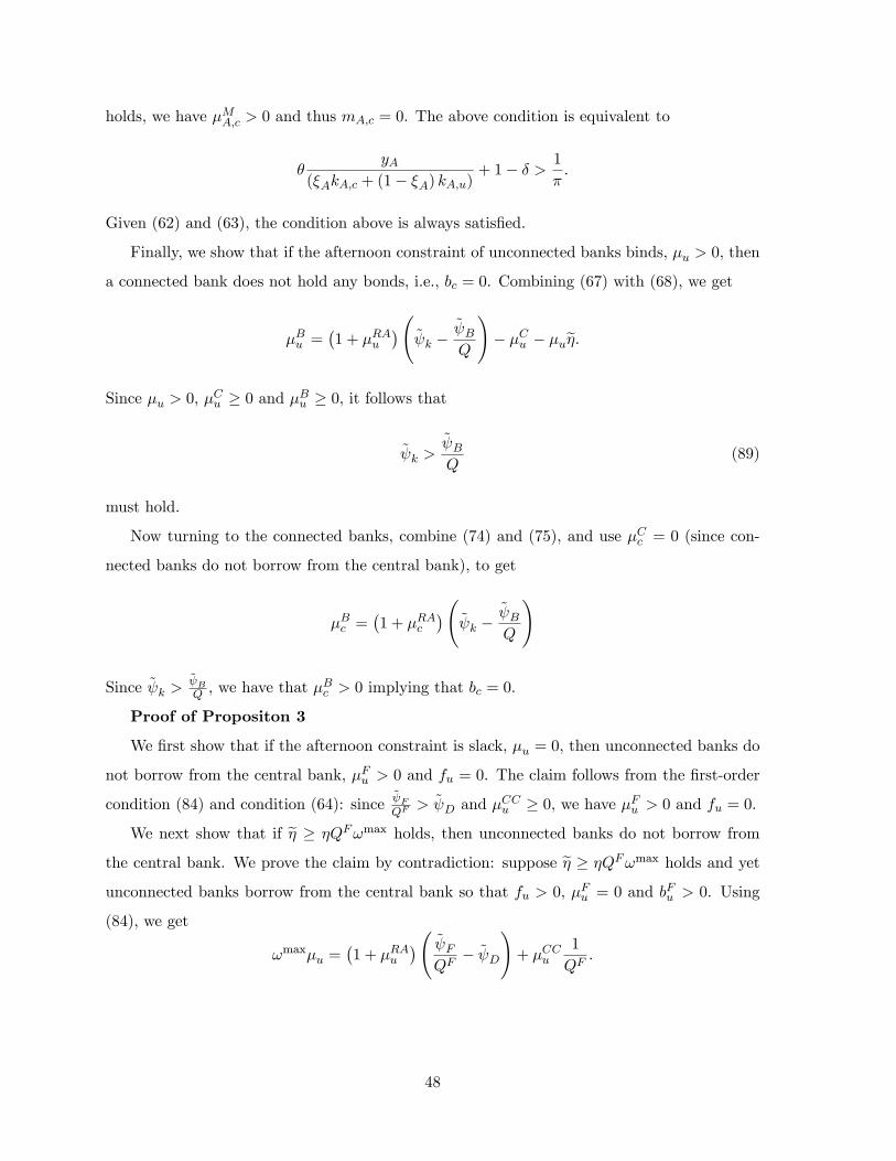
holds, we have µMA,c > 0 and thus mA,c = 0. The above condition is equivalent to

θyA

(ξAkA,c + (1− ξA) kA,u)+ 1− δ > 1

π.

Given (62) and (63), the condition above is always satisfied.

Finally, we show that if the afternoon constraint of unconnected banks binds, µu > 0, then

a connected bank does not hold any bonds, i.e., bc = 0. Combining (67) with (68), we get

µBu =(1 + µRAu

)(ψk −

ψBQ

)− µCu − µuη.

Since µu > 0, µCu ≥ 0 and µBu ≥ 0, it follows that

ψk >ψBQ

(89)

must hold.

Now turning to the connected banks, combine (74) and (75), and use µCc = 0 (since con-

nected banks do not borrow from the central bank), to get

µBc =(1 + µRAc

)(ψk −

ψBQ

)

Since ψk >ψBQ , we have that µ

Bc > 0 implying that bc = 0.

Proof of Propositon 3

We first show that if the afternoon constraint is slack, µu = 0, then unconnected banks do

not borrow from the central bank, µFu > 0 and fu = 0. The claim follows from the first-order

condition (84) and condition (64): since ψFQF

> ψD and µCCu ≥ 0, we have µFu > 0 and fu = 0.

We next show that if η ≥ ηQFωmax holds, then unconnected banks do not borrow from

the central bank. We prove the claim by contradiction: suppose η ≥ ηQFωmax holds and yet

unconnected banks borrow from the central bank so that fu > 0, µFu = 0 and bFu > 0. Using

(84), we get

ωmaxµu =(1 + µRAu

)( ψFQF− ψD

)+ µCCu

1

QF.

48

Since µCu ≥ 0 we have, by (72), that µCCu ≥ µu ηη . Therefore,

ωmaxµu =(1 + µRAu

)( ψFQF− ψD

)+ µCCu

1

QF≥(1 + µRAu

)( ψFQF− ψD

)+ µu

η

η

1

QF

so that

µA,u

(ωmax − η

η

1

QF

)≥(1 + µRAu

)( ψFQF− ψD

).

The right-hand side of the expression above is positive since ψFQF

> ψD by (64). The left-hand

side is non-positive since ωmaxηQF ≤ η. A contradiction.

Finally, we show that if η <ψk−

ψBQ

ψk−ψMholds, then unconnected banks do not borrow in the

secured market and instead they borrow only from the central bank and hold money, mu > 0.

We prove the claim by contradiction: Suppose that η <ψk−

ψBQ

ψk−ψMand yet unconnected banks

use bonds to borrow from the secured market so that bFu < bu and µCu = 0. Since bu > 0, we

have µBu = 0. Since µCu = 0, we have by (72) that µCCu = µuηη . Using this to substitute out

µCCu in (82), we have:

µu =(1 + µRAu

)(ψk −

ψBQ

)1

η

By (83), we have

µMu =(1 + µRAu

) (ψk − ψM

)− µu ≥ 0

so that (1 + µRAu

) (ψk − ψM

)≥ µu.

Then, we have that

(1 + µRAu

) (ψk − ψM

)≥(1 + µRAu

)(ψk −

ψBQ

)1

η

or, equivalently,

η ≥ψk −

ψBQ

ψk − ψM.

A contradiction.

Since unconnected banks borrow from the central bank, their afternoon constraint binds,

µu > 0. Since they do not borrow from the secured market, we have bFu = bu. The binding

49

afternoon constraint then implies that

mu = ωmaxdu > 0.

This completes the proof.

50