Embed Size (px)
Citation preview
The Macroeconomics of AustralianUnemployment
Guy Debelle and James Vickery*
1. IntroductionThe unemployment rate in Australia has risen from less than 2 per cent in the late
1960s to an average of over 8 per cent over the past fifteen years.
In this paper, we examine unemployment from an aggregate perspective and presenta framework with which to analyse how the unemployment rate could be permanentlylowered from its current level. In doing so, we also discuss the role that monetary policycan play in assisting the adjustment to a lower unemployment rate.
A macroeconomic examination of unemployment obscures much of the rich detailthat underpins the labour market. Nevertheless, it enables us to analyse the broad trendsthat have occurred over the past twenty years on both the demand and supply sides of thelabour market. In the next section we examine these trends at an aggregate level. Theaggregate unemployment rate has risen as a result of a large increase in labour supplywhich has not been matched by an equivalent increase in labour demand (employment).Most of the rise in the aggregate unemployment rate occurred in the 1970s, associatedwith the increase in labour costs at that time. Since the early 1980s, the aggregateunemployment rate has fluctuated with the economic cycle around a relatively constantmean.
In Section 2, we also discuss estimates of the natural rate of unemployment. Similarto the trend in the aggregate unemployment rate, the natural rate rose sharply in the mid1970s, but has been relatively steady over the past fifteen years fluctuating between 6 and8 per cent. The adjustment of inflation expectations has played an important role in themovement of the aggregate unemployment rate relative to the natural rate in the 1990s.
An aggregate labour demand and supply curve are at the core of the model describedin Section 3 that provides the foundation for the analysis in the paper. These twoequations are estimated in Section 4 of the paper. The empirical analysis identifies theeffect of real wages and output on labour demand, and the impact of the business cycleon labour supply.
The model presented in Section 3 highlights the importance of the linkage betweenthe level of the aggregate real wage and the unemployment rate. If the aggregate realwage is too high, the unemployment rate will be permanently above its desired level.Consequently, the analysis in Section 5 focuses on the size of the reduction in theunemployment rate that can be achieved by a given reduction in the level of the real wage.It shows that slower real wage growth of 2 per cent below trend for one year could resultin a permanent reduction in the unemployment rate of about one percentage point.
* We thank Philip Lowe, Peter Downes, Jeff Borland, Mardi Dungey, John Pitchford and colleagues at theReserve Bank for helpful discussions.
236 Guy Debelle and James Vickery
The analysis in Section 5 also suggests that monetary policy can play an important rolein the transition to a lower unemployment rate. While monetary policy does not affectthe natural rate of unemployment or potential output, it can help to reduce the transitiontime to the lower unemployment rate, thereby reducing the gap between the actualunemployment rate and the natural rate. It can do so by recognising and correctlyinterpreting the signs of labour market adjustment. The inflation-targeting framework iswell suited to this purpose.
2. A Macroeconomic Overview of the Labour MarketBefore presenting the theoretical framework and the empirical analysis, we first
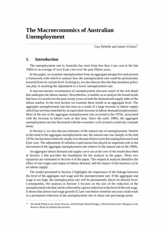
summarise the trends in the key aggregate labour market variables over the pastforty years. Figure 1 suggests that in general, movements in the real cost of employinglabour and the cycles in aggregate demand have been associated with fluctuations inemployment and unemployment. We investigate these relationships more explicitly inSection 4.
Since 1960, the employment to population ratio has fluctuated around a reasonablyconstant mean of around 58 per cent, while the unemployment rate has risen by around
1961 1965 1969 1973 1977 1981 1985 1989 1993 19971961 1965 1969 1973 1977 1981 1985 1989 1993 1997-5
0
5
-5
0
5
-5
0
5
-5
0
5
300
400
500
600
100
105
110
115
300
400
500
600
100
105
110
115
0
5
10
50
55
60
0
5
10
50
55
60
Labour costs
% %
% %GDP growth
Employment and unemployment
Unemployment rate (LHS)
Employment/population (RHS)
Real wages(a)
(LHS)
Real unit labour costs(b)
(RHS)
Figure 1: An Aggregate Overview of the Labour Market
Notes: (a) $/week; 1989–90 prices.
(b) Index; 1966–67 to 1972–73 = 100.
237The Macroeconomics of Australian Unemployment
6 percentage points. This definitionally implies that the growth in labour demand has notkept pace with the growth in labour supply, particularly over the past 25 years. Thedriving force behind the increase in labour supply has been the increased participationof females which has more than offset a slow decline in the male participation rate(Borland and Kennedy 1998).
The rise in the participation rate need not have led to a rise in the aggregateunemployment rate, provided there was a decline in the real wage to enable the labourmarket to absorb the increased supply. This decline would not necessarily be permanent– in a standard trade model, in the long run, the returns paid to factors of production areinvariant to the supply of those factors. However, in actuality, as is discussed in the restof this section, the reverse occurred, namely the real wage increased at the same time asthe increase in supply.
Increases in the unemployment rate occurred primarily in three relatively shortperiods. The first of these was in the mid 1970s and was associated with a sharp rise inlabour costs. After the rapid rise in average weekly earnings in 1974 of 28 per cent, realunit labour costs remained at historically high levels until the early 1980s. This rise inlabour costs was associated with a five percentage point fall in the employment topopulation ratio and an increase in the unemployment rate of nearly 4 percentage points.1
The unemployment rate increased further around 1982 following the wage pushassociated with the resources boom of the early 1980s (when average weekly earningsrose at an annual rate of 14 per cent in the two years to June 1982) and as a result of the1982–83 recession. The wage rise in this case was relatively short-lived, but theunemployment rate rose by 4 percentage points and the employment to population ratiofell by 2 percentage points. In the second half of the 1980s, during the Price and IncomesAccords, real unit labour costs fell below their levels of the early 1970s and employmentrose steadily.2 However, despite the recovery of the employment to population ratio toits level of the early 1970s, the unemployment rate did not fall much below 6 per cent.This was a result of the increase in the participation rate of over 3 percentage pointsbetween 1984 and 1990.
Finally, the unemployment rate rose again in the early 1990s following the recessionat that time. Subsequently, the employment to population ratio has recovered to aroundits average level, and the unemployment rate has fallen back to its current level of around8 per cent.
The sharp rises and the subsequent slow declines in the unemployment rate highlightthe costs of large cycles in output and the benefits of maintaining steady growth(Macfarlane 1997). In previous work, we have shown that if the Phillips curve isnon-linear, the more stable the path of economic growth, the lower the average rate ofunemployment (Debelle and Vickery 1997). A consistent rate of economic growth close
1. At the time, there was a vigorous debate about the impact of these wage movements on employment – the‘real wage overhang’ debate. See Chapman (1990), Gregory and Duncan (1979) and Indecs (1986) for asummary of the debate.
2. A similar debate has occurred on the role of the Accord in the observed wage outcomes over this time.Cockerell and Russell (1995) and Pissarides (1991) find no impact of the Accord on wages once otherinfluences are accounted for, whereas Chapman and Gruen (1990) and Watts and Mitchell (1990)conclude the opposite.
238 Guy Debelle and James Vickery
to the trend growth rate of the economy will ensure that the unemployment rate remainsclose to the natural rate of unemployment through time, thereby lowering the averageunemployment rate. On the other hand, a Schumpeterian view of the world wouldsuggest that there are long-run benefits to economic growth from economic cycles.Caballero and Hammour (1996), however, show that even in this case, large volatility ineconomic growth is likely to be detrimental.
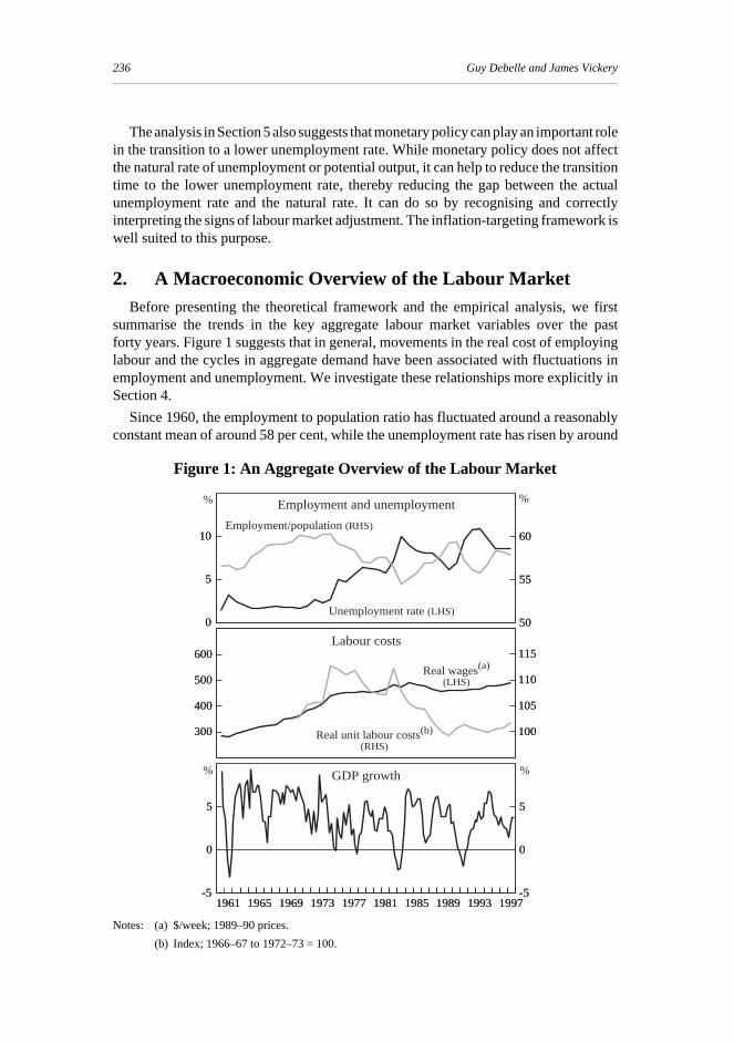
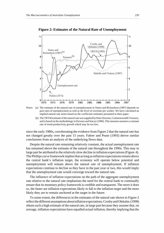
A standard decomposition of the aggregate unemployment rate is into its cyclical andstructural components. The structural or natural rate of unemployment is that levelassociated with a constant and expected inflation rate, given the institutional structure ofthe economy. Figure 2 shows some estimates of the natural rate in Australia. Theseestimates are clearly quite divergent, reflecting, inter alia, the different techniques theauthors have employed and the different sample periods used in the estimation.
The time series of aggregate unemployment shown in Figure 2 suggests that thenatural rate has risen since the early 1970s, but has been relatively constant since the early1980s. This is supported by Debelle and Vickery’s (1997) estimate of the natural rate,which rises sharply in the mid 1970s, and the natural rate series in the TRYM modelwhich has a once-off level shift in 1974 of around 21/2 percentage points (CommonwealthTreasury 1996).
The large movements in the natural rate are generally associated with large movementsin real wages: the rise in the natural rate in the mid 1970s occurred at the same time asthe large shock to the real wage. Similarly, the decline in Debelle and Vickery’s estimateof the natural rate in the late 1980s was associated with the moderation in real wagegrowth.
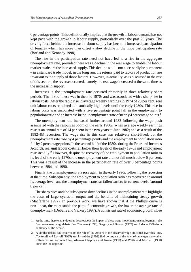
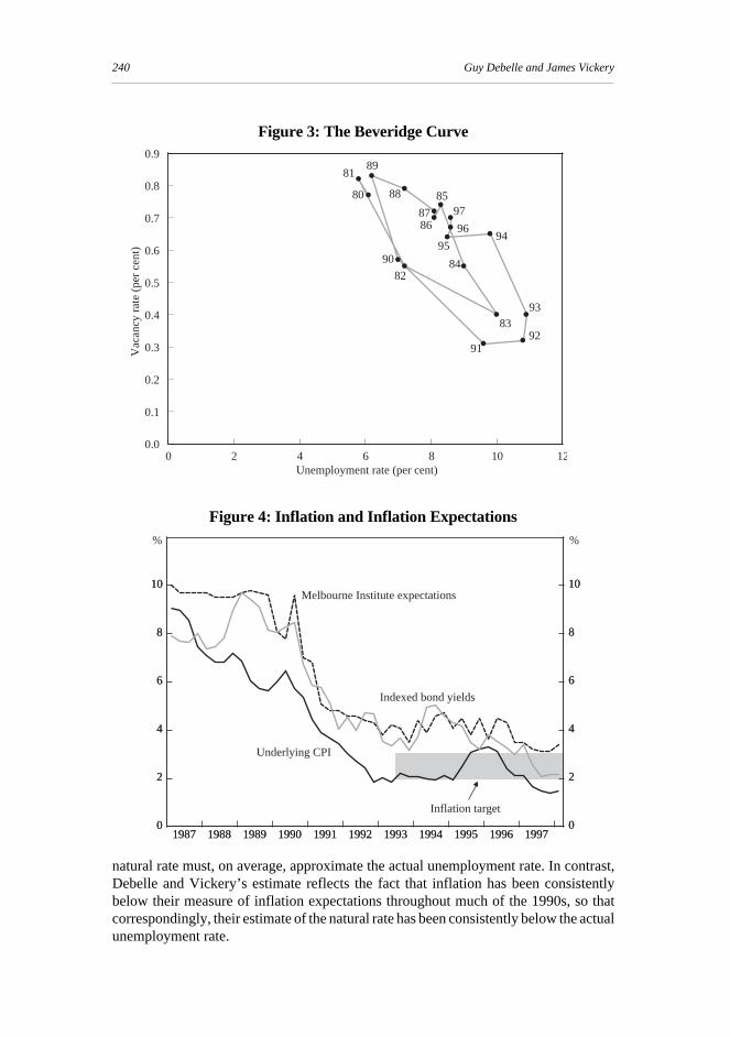
A number of microeconomic factors are also likely to have influenced the path of thenatural rate, including factors that affect a person’s willingness to search for a job suchas the level of unemployment benefits and the location of job opportunities. However,it has generally proven difficult to directly relate the rise in the natural rate to specificcauses, in part because of the difficulty in estimating the natural rate itself. An indirectguide to movements in the natural rate can be obtained by examining factors that havecaused shifts in the Beveridge curve which plots the rate of unemployment against thelevel of job vacancies (Figure 3).3 The negative slope of the curve is evident, reflectingthe fact that in booms, new jobs are being created at a faster pace and there are lessunemployed people looking for jobs, while in recessions, the converse is true.
Underpinning the stocks of unemployed people and job vacancies each period arelarge flows into and out of employment and unemployment. Changes in the efficiencywith which the large flows of workers are matched with vacancies shift the position ofthe Beveridge curve, while over the business cycle the economy shifts along theBeveridge curve.
Using data from 1980 onwards, we estimate the Beveridge curve for Australia inAppendix A. We test to see whether different indicators of the efficiency of process thatmatches job seekers and job vacancies have led to shifts in the Beveridge curve but findlittle evidence of this. This suggests that the Beveridge curve has not shifted outwards
3. Reliable vacancies data are not available prior to 1979. However, it appears likely that the Beveridge curveshifted outwards during the 1970s (Harper 1980).
239The Macroeconomics of Australian Unemployment
since the early 1980s, corroborating the evidence from Figure 2 that the natural rate hasnot changed greatly over the past 15 years. Fahrer and Pease (1993) derive similarconclusions from an analysis of the underlying flows data.
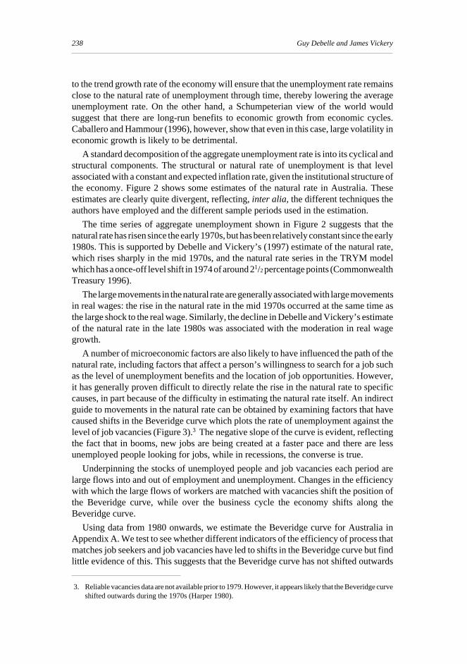
Despite the natural rate remaining relatively constant, the actual unemployment ratehas remained above the estimate of the natural rate throughout the 1990s. This may inlarge part be attributed to the relatively slow decline in inflation expectations (Figure 4).The Phillips curve framework implies that as long as inflation expectations remain abovethe central bank’s inflation target, the economy will operate below potential andunemployment will remain above the natural rate of unemployment. If inflationexpectations continue to decline as they have in the past year or two, this would implythat the unemployment rate would converge toward the natural rate.
The influence of inflation expectations on the path of the aggregate unemploymentrate relative to the natural rate emphasises the need for the central bank to continuallyensure that its monetary policy framework is credible and transparent. The more it doesso, the faster are inflation expectations likely to fall to the inflation target and the morelikely they are to remain anchored at the target in the future.
To some extent, the differences in the estimates of the natural rate shown in Figure 2reflect the different assumptions about inflation expectations. Crosby and Olekalns (1998)obtain such a high estimate of the natural rate, in large part because they assume that, onaverage, inflation expectations have equalled actual inflation, thereby implying that the
Figure 2: Estimates of the Natural Rate of Unemployment
Notes: (a) The estimate of the natural rate of unemployment in Simes and Richardson (1987) depends onpast rates of unemployment as well as the level of overtime per worker. We have calculated animplied natural rate series based on the coefficient estimates presented in their paper.
(b) The TRYM estimate of the natural rate was supplied by Peter Downes, Commonwealth Treasury,and is based on the methodology in Downes and Stacey (1996). This measure assumes a constantrate of trend productivity growth which may be too low.
1970 1973 1976 1979 1982 1985 1988 1991 1994 19971970 1973 1976 1979 1982 1985 1988 1991 1994 19970
2
4
6
8
10
0
2
4
6
8
10
0
2
4
6
8
10
0
2
4
6
8
10
Richardson (1987)(a)
% %
Treasury(b)
Parkin (1973)
Crosby andOlekalns (1998)
Debelle and Vickery (1997)
Unemployment rate
OECD (1995)Simes and
240 Guy Debelle and James Vickery
Figure 3: The Beveridge Curve
Figure 4: Inflation and Inflation Expectations
l
l
l
l
l
l
ll
l
l
l
l l
l
llll
0.0
0.1
0.2
0.3
0.4
0.5
0.6
0.7
0.8
0.9
0 2 4 6 8 10 12
Vac
ancy
rat
e (p
er c
ent)
Unemployment rate (per cent)
80
81
82
83
84
85
8687
88
89
90
9192
93
9495
96
97
1987 1988 1989 1990 1991 1992 1993 1994 1995 1996 19971987 1988 1989 1990 1991 1992 1993 1994 1995 1996 19970
2
4
6
8
10
0
2
4
6
8
10
0
2
4
6
8
10
0
2
4
6
8
10
Indexed bond yields
% %
Melbourne Institute expectations
Underlying CPI
Inflation target
natural rate must, on average, approximate the actual unemployment rate. In contrast,Debelle and Vickery’s estimate reflects the fact that inflation has been consistentlybelow their measure of inflation expectations throughout much of the 1990s, so thatcorrespondingly, their estimate of the natural rate has been consistently below the actualunemployment rate.
241The Macroeconomics of Australian Unemployment
The OECD (1996) estimate is derived from a wage, rather than a price, Phillips curve,and suffers from the problem that it ignores productivity growth. A trend increase inproductivity growth, which is in part reflected in higher wages, will cause the estimateof the natural rate to increase, despite the absence of any inflationary pressure. As therehas been an increase in average productivity growth in the 1990s, the OECD measure ofthe natural rate is above most other measures.
In summary, the aggregate data suggest that there is a strong relationship betweenmovements in real wages and output, and trends in employment and unemployment (weestimate these relationships in Section 4). The large shift upwards in the natural rate ofunemployment in the mid 1970s coincided with a rapid increase in labour costs.Subsequently the natural rate has fluctuated around a higher rate of about 7 per cent. Inrecent years, the actual unemployment rate has remained above estimates of the naturalrate, in large part because inflation expectations have only slowly fallen towards thetargeted inflation rate.
3. An Aggregate Model of the Labour MarketIn this section, we describe a simple framework to examine unemployment from a
macroeconomic perspective. Here we present the steady-state version of the model,while later, in Section 5, we add some dynamics to examine the role for monetary policyin assisting the process of labour market adjustment.
In order to address the issue of unemployment, the model requires a departure fromthe standard neoclassical framework where full employment is generally automaticallyattained in the long run. Rather, the model is similar to the imperfect competition modelof the labour market developed by Layard and Nickell (1986), or the insider/outsidermodel of Lindbeck and Snower (1988).
Output is produced using two factors, capital (k) and labour (e),4 so that theeconomy-wide production function is given by:
y f k es = ( , ) (1)
In equilibrium, the output supplied by firms equals the output demanded. If not, thereis a change in inventory levels. However, we will ignore the role of inventories andassume that output demanded always equals output supplied:
y y yd s= = (2)
Output will differ from the level of potential output (y*) if either the real interest rate(r), the instrument of monetary policy, deviates from its equilibrium value (r ), orthrough the impact of fiscal policy (fp). To focus on the role of monetary policy, we willassume hereafter that fp=0.
y y r r fp− = − +* ( )ξ (3)
4. Lower-case letters denote logs, upper-case letters, levels.
242 Guy Debelle and James Vickery
Turning to the labour market, the number of unemployed people U is definitionallyequal to the labour force L less the number of those employed E, so the unemploymentrate u can be written as:
u EL≡ −1 (4)
The employment demand equation is derived from the cost minimisation decision ofthe firm (in this case the economy):5
e y w c= − +δ η θ (5)
where w is the real wage, c is the real user cost of capital, and η denotes theconstant-output elasticity of labour demand.6 This elasticity is the percentage change inemployment for a one percentage point change in the real wage, holding output (and thecost of capital) constant. The total effect of a change in the real wage on employment,however, will depend on the extent to which output also changes in response to thechange in the real wage (the ‘scale effect’). A fall in the real cost of labour results in thesubstitution of labour for capital in production. In addition, the firm (economy) is ableto move to a higher level of production, thereby employing more labour and more capital.
The existence of the scale effect assumes that there are underutilised resources in theeconomy. If the unemployment rate is at the frictional unemployment rate (that is,unemployed workers are simply in transition from one employment opportunity toanother), then a reduction in the real wage would likely be reversed by the resultantlabour market pressure.
The demand for capital is similarly derived from the cost minimisation decision:
k y w c= + −τ ψ λ (6)
The labour supply curve is an aggregate of individuals’ labour supply decisions. Itdepends on the real wage reflecting the labour-leisure choice, and is also assumed todepend on the state of the economy through the encouraged worker effect: when the rateof unemployment is lower, people are more willing to look for work as they expect theprobability of finding employment to be greater.
l u w= − +κ σ (7)
We adopt the simple specification that wages depend on an exogenous component,and the gap between the rate of unemployment and the natural rate of unemployment (u*)which captures the effect of the tightness of the labour market on the level of real wages.This is similar to the wage-setting curve in the Layard-Nickell (1986) model and can bederived from the Shapiro-Stiglitz (1984) model of efficiency wages or theLindbeck-Snower (1988) model. The exogenous component may reflect the relativebargaining power of insiders and outsiders in the labour market, or the relativebargaining strengths of workers and firms.
w w u u= ′ − −ζ ( *) (8)
5. For a full treatment see Hamermesh (1993).
6. η is not necessarily the firm-level elasticity of labour demand because of issues of aggregation(Hamermesh 1993, p. 64). Thus the estimates of η obtained in Section 4 below are not directly comparablewith those obtained from microeconomic studies.
243The Macroeconomics of Australian Unemployment
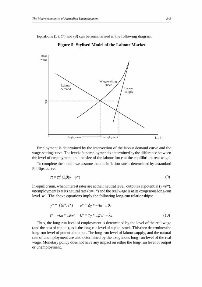
Equations (5), (7) and (8) can be summarised in the following diagram.
Figure 5: Stylised Model of the Labour Market
w
Realwage
Wage-settingcurveLabour
demand Laboursupply
UnemploymentEmployment L , LDS
p
Employment is determined by the intersection of the labour demand curve and thewage-setting curve. The level of unemployment is determined by the difference betweenthe level of employment and the size of the labour force at the equilibrium real wage.
To complete the model, we assume that the inflation rate is determined by a standardPhillips curve:
π π β= + −e y y( *) (9)
In equilibrium, when interest rates are at their neutral level, output is at potential (y=y*),unemployment is at its natural rate (u=u*) and the real wage is at its exogenous long-runlevel ′w . The above equations imply the following long-run relationships:
y f k e* ( *, *)≡ e y w c* *= − ′ +δ η θ
l u w* *= − + ′κ σ k y w c* *= + ′ −τ ψ λ (10)
Thus, the long-run level of employment is determined by the level of the real wage(and the cost of capital), as is the long-run level of capital stock. This then determines thelong-run level of potential output. The long-run level of labour supply, and the naturalrate of unemployment are also determined by the exogenous long-run level of the realwage. Monetary policy does not have any impact on either the long-run level of outputor unemployment.
244 Guy Debelle and James Vickery
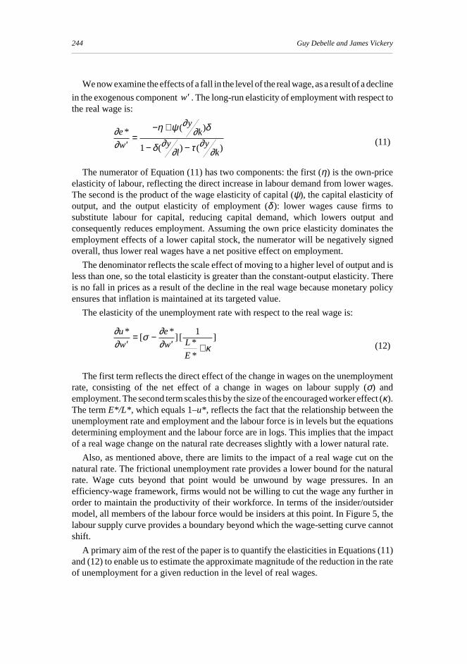
We now examine the effects of a fall in the level of the real wage, as a result of a decline
in the exogenous component ′w . The long-run elasticity of employment with respect tothe real wage is:
∂∂
η ψ ∂∂ δ
δ ∂∂ τ ∂
∂
e
w
yk
yl
yk
* ( )
( ) ( )′=
− +
− −1(11)
The numerator of Equation (11) has two components: the first (η) is the own-priceelasticity of labour, reflecting the direct increase in labour demand from lower wages.The second is the product of the wage elasticity of capital (ψ), the capital elasticity ofoutput, and the output elasticity of employment (δ ): lower wages cause firms tosubstitute labour for capital, reducing capital demand, which lowers output andconsequently reduces employment. Assuming the own price elasticity dominates theemployment effects of a lower capital stock, the numerator will be negatively signedoverall, thus lower real wages have a net positive effect on employment.
The denominator reflects the scale effect of moving to a higher level of output and isless than one, so the total elasticity is greater than the constant-output elasticity. Thereis no fall in prices as a result of the decline in the real wage because monetary policyensures that inflation is maintained at its targeted value.
The elasticity of the unemployment rate with respect to the real wage is:
∂∂
σ ∂∂ κ
u
w
e
w L
E
*[
*] [ *
*
]′
= −′ +
1
(12)
The first term reflects the direct effect of the change in wages on the unemploymentrate, consisting of the net effect of a change in wages on labour supply (σ) andemployment. The second term scales this by the size of the encouraged worker effect (κ).The term E*/L* , which equals 1–u*, reflects the fact that the relationship between theunemployment rate and employment and the labour force is in levels but the equationsdetermining employment and the labour force are in logs. This implies that the impactof a real wage change on the natural rate decreases slightly with a lower natural rate.
Also, as mentioned above, there are limits to the impact of a real wage cut on thenatural rate. The frictional unemployment rate provides a lower bound for the naturalrate. Wage cuts beyond that point would be unwound by wage pressures. In anefficiency-wage framework, firms would not be willing to cut the wage any further inorder to maintain the productivity of their workforce. In terms of the insider/outsidermodel, all members of the labour force would be insiders at this point. In Figure 5, thelabour supply curve provides a boundary beyond which the wage-setting curve cannotshift.
A primary aim of the rest of the paper is to quantify the elasticities in Equations (11)and (12) to enable us to estimate the approximate magnitude of the reduction in the rateof unemployment for a given reduction in the level of real wages.
245The Macroeconomics of Australian Unemployment
4. Labour Demand and SupplyIn this section we estimate the equations for labour demand and supply that form the
foundation of the model in Section 3.
4.1 Labour demand
As described in Section 3, the basic form of the labour demand equation that weestimate is derived from the cost minimisation decision of the representative firm (thedual of the profit maximisation decision):
e L y w c ad= ( , , , ) (5′)
where Equation (5) is extended to take account of a, the level of productivity.
A labour demand curve similar to Equation (5′) can also be derived from an imperfectcompetition framework, where each firm faces a downward-sloping demand curve fortheir product, and sets output prices based on expectations of future aggregate prices(Barrell, Pain and Young 1996). Layard and Nickell (1986) derive a somewhat differentlabour demand equation which controls for the capital stock rather than the level ofoutput. Hamermesh (1993) refers to the Layard-Nickell specification as a short-runlabour demand curve in that it captures changes in the demand for labour before thecapital stock adjusts. In addition to this theoretical consideration, the problems ofmeasuring the capital stock lead us to adopt a specification that controls for the level ofoutput rather than capital.
Sargent (1978) extends the static labour demand model described in Equation (5′) byassuming that the firm faces costs in adjusting the level of employment, resulting in apartial-adjustment specification. Furthermore, the non-stationarity of the variablesinfluencing equilibrium employment suggests that an error-correction framework is theappropriate way to model aggregate labour demand (Amano and Wirjanto 1997), andthis is the approach that we adopt.
The core variables of interest in our labour demand equation are employment, realwages, output and the user cost of capital. We do not make an explicit distinction betweenemployment and labour demand in our modelling work, obviating the need to estimatea separate equation linking these two concepts. This contrasts with the labour demandequation in the TRYM model which measures labour demand as the sum of employmentand vacancies (Commonwealth Treasury 1996). Since our Beveridge curve regressionin Appendix A suggests that the relationship between unemployment and vacancies hasnot shifted over our sample period, and given that it is difficult to translate vacancies intoan hours equivalent, we use actual employment, measured by aggregate hours workedin the non-farm economy, as the dependent variable (hours) in the labour demandequation.
The real wage measure (wage) is total labour costs per hour, which takes into accountpayroll tax, superannuation contributions and fringe benefits tax in addition to the hourlywage rate, deflated by the non-farm GDP deflator. Output is measured by non-farmGDP(A) and the user cost of capital (ucc) is constructed as a weighted average of the realcost of debt and equity. A full definition of each variable is provided in Appendix B.
246 Guy Debelle and James Vickery
We include a linear trend to capture labour productivity. We also tried a measure ofmulti-factor productivity (MFP), calculated as a weighted average of labour and capitalproductivity, but found that the variable was generally insignificant and of the wrongsign. In part this may be because MFP is affected by cyclical factors, in particular, thelevel of capital utilisation. When we included both a time trend and multi-factorproductivity in the equation, the time trend was significant whereas MFP was not.
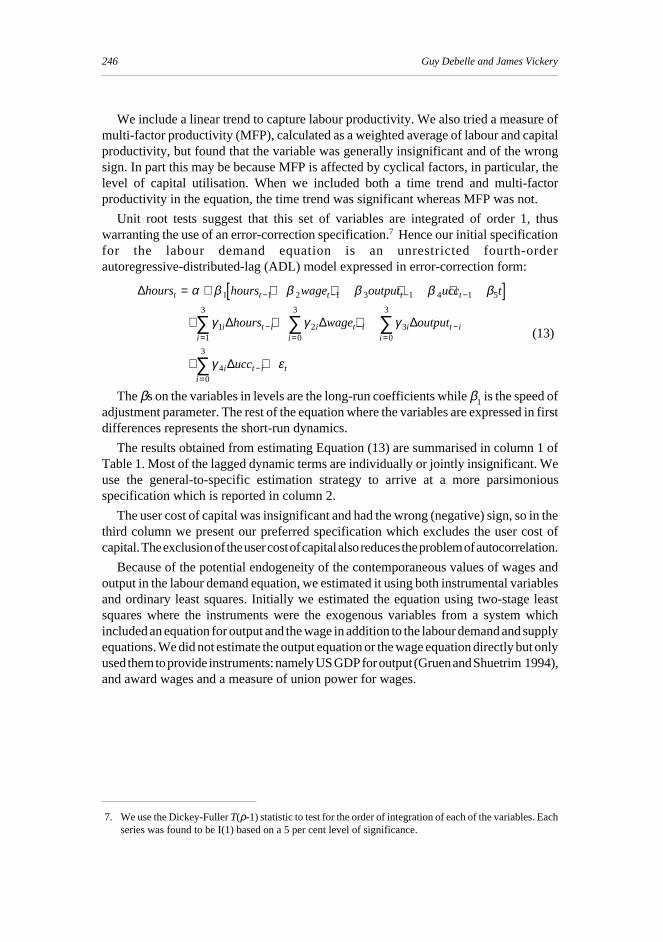
Unit root tests suggest that this set of variables are integrated of order 1, thuswarranting the use of an error-correction specification.7 Hence our initial specificationfor the labour demand equation is an unrestricted fourth-orderautoregressive-distributed-lag (ADL) model expressed in error-correction form:
(13)
The βs on the variables in levels are the long-run coefficients while β1 is the speed ofadjustment parameter. The rest of the equation where the variables are expressed in firstdifferences represents the short-run dynamics.
The results obtained from estimating Equation (13) are summarised in column 1 ofTable 1. Most of the lagged dynamic terms are individually or jointly insignificant. Weuse the general-to-specific estimation strategy to arrive at a more parsimoniousspecification which is reported in column 2.
The user cost of capital was insignificant and had the wrong (negative) sign, so in thethird column we present our preferred specification which excludes the user cost ofcapital. The exclusion of the user cost of capital also reduces the problem of autocorrelation.
Because of the potential endogeneity of the contemporaneous values of wages andoutput in the labour demand equation, we estimated it using both instrumental variablesand ordinary least squares. Initially we estimated the equation using two-stage leastsquares where the instruments were the exogenous variables from a system whichincluded an equation for output and the wage in addition to the labour demand and supplyequations. We did not estimate the output equation or the wage equation directly but onlyused them to provide instruments: namely US GDP for output (Gruen and Shuetrim 1994),and award wages and a measure of union power for wages.
7. We use the Dickey-Fuller T(ρ-1) statistic to test for the order of integration of each of the variables. Eachseries was found to be I(1) based on a 5 per cent level of significance.
∆
∆ ∆ ∆
∆
hours hours wage output ucc t
hours wage output
ucc
t t t t t
ii
t i ii
t i ii
t i
ii
t i t
= + + + + +[ ]+ + +
+ +
− − − −
=−
=−
=−
=−
∑ ∑ ∑
∑
α β β β β β
γ γ γ
γ ε
1 1 2 1 3 1 4 1 5
11
3
20
3
30
3
40
3
247The Macroeconomics of Australian Unemployment
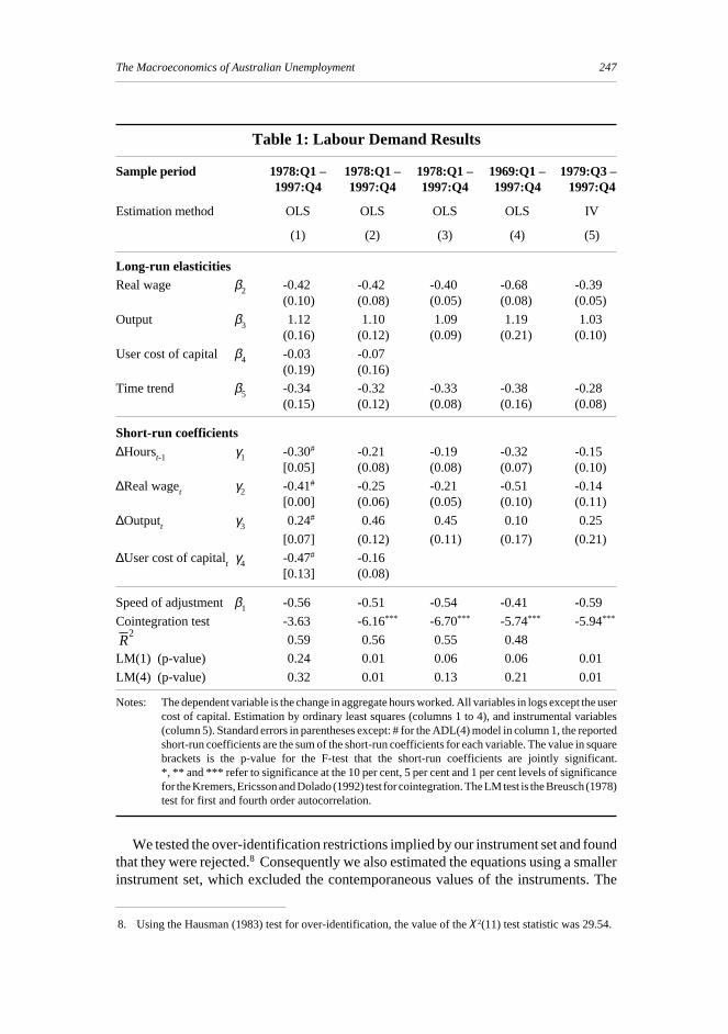
Table 1: Labour Demand Results
Sample period 1978:Q1 – 1978:Q1 – 1978:Q1 – 1969:Q1 – 1979:Q3 –1997:Q4 1997:Q4 1997:Q4 1997:Q4 1997:Q4
Estimation method OLS OLS OLS OLS IV
(1) (2) (3) (4) (5)
Long-run elasticitiesReal wage β2 -0.42 -0.42 -0.40 -0.68 -0.39
(0.10) (0.08) (0.05) (0.08) (0.05)
Output β3 1.12 1.10 1.09 1.19 1.03(0.16) (0.12) (0.09) (0.21) (0.10)
User cost of capital β4 -0.03 -0.07(0.19) (0.16)
Time trend β5 -0.34 -0.32 -0.33 -0.38 -0.28(0.15) (0.12) (0.08) (0.16) (0.08)
Short-run coefficients∆Hourst-1 γ1 -0.30# -0.21 -0.19 -0.32 -0.15
[0.05] (0.08) (0.08) (0.07) (0.10)
∆Real waget γ2 -0.41# -0.25 -0.21 -0.51 -0.14[0.00] (0.06) (0.05) (0.10) (0.11)
∆Outputt γ3 0.24# 0.46 0.45 0.10 0.25
[0.07] (0.12) (0.11) (0.17) (0.21)
∆User cost of capitalt γ4 -0.47# -0.16[0.13] (0.08)
Speed of adjustmentβ1 -0.56 -0.51 -0.54 -0.41 -0.59
Cointegration test -3.63 -6.16*** -6.70*** -5.74*** -5.94***
R2
0.59 0.56 0.55 0.48
LM(1) (p-value) 0.24 0.01 0.06 0.06 0.01
LM(4) (p-value) 0.32 0.01 0.13 0.21 0.01
Notes: The dependent variable is the change in aggregate hours worked. All variables in logs except the usercost of capital. Estimation by ordinary least squares (columns 1 to 4), and instrumental variables(column 5). Standard errors in parentheses except: # for the ADL(4) model in column 1, the reportedshort-run coefficients are the sum of the short-run coefficients for each variable. The value in squarebrackets is the p-value for the F-test that the short-run coefficients are jointly significant.*, ** and *** refer to significance at the 10 per cent, 5 per cent and 1 per cent levels of significancefor the Kremers, Ericsson and Dolado (1992) test for cointegration. The LM test is the Breusch (1978)test for first and fourth order autocorrelation.
We tested the over-identification restrictions implied by our instrument set and foundthat they were rejected.8 Consequently we also estimated the equations using a smallerinstrument set, which excluded the contemporaneous values of the instruments. The
8. Using the Hausman (1983) test for over-identification, the value of the χ 2(11) test statistic was 29.54.
248 Guy Debelle and James Vickery
results of this estimation are reported in column 5 of Table 1. A Hausman test failed toreject the null hypothesis of exogeneity using either instrument set,9 so we focus on theOLS estimates in the remainder of the discussion. As column 5 indicates, the results arelittle changed if IV is used. Quandt and Rosen (1989) also found that endogenising outputmade little difference to coefficient estimates in an aggregate labour demand curve forthe United States, and that exogeneity of output could not be rejected statistically.
We estimate the equation over two time horizons. Columns 1, 2, 3 and 5 use data from1978:Q1 to 1997:Q4 where labour demand is measured by the aggregate hours workedin the non-farm economy. As this series is not available before 1978, column 4 uses datafrom 1969:Q1 to 1997:Q4, measuring labour demand by aggregate hours worked in thewhole economy adjusted for the share of non-farm output in total output. Hours workedin the non-farm economy is less volatile than that in the whole economy thus accounting,in part, for the lower explanatory power in column 4.
Our estimate of the long-run real wage elasticity of employment of -0.4 is smaller thanthe previous estimates of around -0.8 (Lewis and Kirby 1988; Pissarides 1991; Russelland Tease 1991). Our estimates lie inside the range of -0.15 to -0.75 that Hamermesh (1993)reports in his survey of the international labour demand literature as ‘a reasonableconfidence interval’ for the real wage elasticity.
The difference between our estimates and the other Australian studies appears to bepartially due to the sample period used, and partially a result of different modelspecifications.10 When we estimate the model over the longer period (column 4), we finda significantly higher wage elasticity of -0.67. To examine how the wage elasticity hasevolved over time, we estimated rolling regressions of the labour demand equation overfifteen-year windows. This indicates that the wage elasticity has declined (in absolutevalue) since the mid 1980s but has been relatively constant over the 1990s at around -0.4.Furthermore, Russell and Tease use real unit labour costs as their measure of labour costs.In the appendix to their paper they report a specification that uses a measure of real wageswhich yields a significantly lower wage elasticity of -0.36.
Our estimate of the long-run output elasticity is, however, consistent with previousestimates. The output elasticity is not significantly different from one in either the shorteror longer sample, implying that a one per cent increase in output leads to a one per centincrease in employment. The TRYM model actually imposes a unitary elasticity ratherthan estimates it.
The speed of adjustment to long-run equilibrium is generally invariant to thespecification used. The estimate of around 0.5 implies that 95 per cent of the adjustmentback towards long-run equilibrium is completed within four quarters after a shock. Thespecifications in Table 1 all assume that the speed of adjustment is constant. We alsoestimated a specification of the labour demand curve where the speed of adjustmentdepends on the tightness of the labour market and hiring and firing costs (Burgess 1993).However, the evidence suggested that the speed of adjustment is invariant to the state ofthe business cycle.
9. The value of the χ 2(8) test statistic was 2.76.
10. The differences are not due to the measure of wages that we use. A similar long-run elasticity was obtainedusing a number of different wage measures.
249The Macroeconomics of Australian Unemployment
In summary, our preferred specification for labour demand contains only real labourcosts, output, and a linear trend. The constant-output real wage elasticity appears to bearound -0.4, while the output elasticity is around 1.
4.2 Labour supply
The labour supply or participation rate equation can be derived from an aggregateversion of the individual’s labour/leisure choice, in which labour supply is determinedby the wage, the prices of goods in an individual’s consumption basket, and non-wageincome. An individual will supply labour, provided that the payoff from acceptingemployment exceeds their reservation wage.
We measure the consumption wage (cwage) using after-tax average weekly earningsdeflated by the consumer price index, and also include in the specification the real levelof unemployment benefits (ben) which is likely to have a major influence on thereservation wage.
In the basic labour supply model, the real consumption wage represents the payoff forthe individual supplying labour to the market. However, if there is uncertainty about theprospects of obtaining employment, the probability of finding work will also affect thepayoff. Consequently, the participation rate tends to be pro-cyclical as a result of this‘discouraged/encouraged’ worker effect.
On the other hand, viewing the labour supply decision from the household level, amajor component of an individual’s non-wage income is the income of their spouse. Iftheir spouse loses their job as the economy enters a downturn, an individual may enterthe labour force to offset the decline in household income. This ‘added’ worker effectwill dampen the discouraged worker effect. However, Bradbury (1995) finds littleevidence for a significant added worker effect using Australian Department of SocialSecurity data.
A review of early Australian models of aggregate labour supply is provided in Dunlop,Healy and McMahon (1984). They find that in many of the studies surveyed, keyparameter estimates were unstable over time, and that the model specifications used werenot linked closely enough to economic theory. Since that time, much of the macroeconomicresearch on labour force participation has focused on separating trend and cyclicalinfluences on labour supply (Dixon 1996; Dowrick 1988; Gregory 1991), rather thanmodelling labour supply decisions in terms of behavioural variables.
Most of the relevant existing literature on participation rates uses the employment topopulation ratio to capture the discouraged worker effect (e.g. Dowrick 1988; Elmeskovand Pichelmann 1993; Pissarides 1991; Stacey and Downes 1995). However, there is adefinitional link between the employment to population ratio and the participation rate:
Labour Force/Population = Employed/Population + Unemployed/Population
Any divergence between the two occurs only because of changes in the unemploymentrate. Consequently, the direction of causality between the two variables is unclear.Elmeskov and Pichelman suggest that the main linkage runs from employment toparticipation, although they acknowledge that the causality is most probably bi-directional.If an exogenous increase in labour supply increases employment by putting downwardpressure on wages, then the employment to population variable is rendered endogenousin a participation rate equation.
250 Guy Debelle and James Vickery
The critical factor in the labour supply decision is the expected probability of findingemployment. Therefore we measure the discouraged worker effect using the vacancyrate (vac), or the vacancy rate relative to the pool of unemployed (vacu).
We estimate separate equations for male and female participation rates, reflectingtheir divergent behaviour over the sample period. The lower participation rates of womenand the higher proportion of women in part-time employment has historically beenindicative of a more marginal attachment to the labour force. Thus, we might expect theirparticipation to be more sensitive to the discouraged worker effect. For married womenwith children, child care costs may also influence their labour supply decision, so weinclude the ratio of child care costs to female average weekly earnings (child) in thefemale participation rate equation. We also test for the impact of housing loan affordability(home) on female labour supply as suggested by Connolly and Spence (1996).
A major change which has influenced the supply decision of both genders over thesample period has been the increase in school retention rates and the increasedparticipation in tertiary education. We control for this effect using the proportion of menand women in full-time education (edu).
However, some part of the trends in male and female participation may reflect changesin social preferences which we are unable to model directly, so we also include a timetrend in both specifications. Thus our general specification for the participation rateequation for each gender is given by:
∆
∆ ∆
∆ ∆ ∆
pr pr vac cwage ben child
edu e t pr vac
cwage ben child
t t t t t t
t t t i t ii
i t ii
i t ii
i
= + + + +
+ + + + +
+ + +
− − − − −
− − − −=
−=
−=
∑
∑ ∑
φ φ φ φ φ
φ φ φ δ δ
δ δ δ
1 1 2 1 3 1 4 1 5 1
6 1 7 1 8 1 1 20
1
30
1
40
1
5
[
]hom
tt ii
i t ii
i t ii
tedu e a
−=
−=
−=
∑
∑ ∑+ + + +
0
1
60
1
70
1
δ δ ε∆ ∆hom
(14)
The expression in the square brackets describes the long-run relationship, with φ1 thespeed of adjustment parameter while the short-run dynamics are described in the rest ofthe equation.11
The model is estimated using quarterly data from 1979:Q3 to 1997:Q4. As in thelabour demand equation, we initially used instrumental variables estimation to allow forthe possibility of endogeneity of the vacancy rate and the wage. However, again aHausman test failed to reject the hypothesis of exogeneity,12 so in Table 2, we report theresults from estimating the equation using ordinary least squares. The lagged dynamicterms were insignificant so the first column for each gender reports the results with onlycontemporaneous dynamic terms.
11. The male and female participation rates, and each of the right-hand side variables, were found to be I(1)at the 5 per cent level of significance, based on the Dickey-Fuller T(ρ-1) test.
12. The value of the Hausman χ 2(9) test statistic was 1.88 for the male participation rate equation, andχ 2(9) = 2.73 for the female participation rate equation.
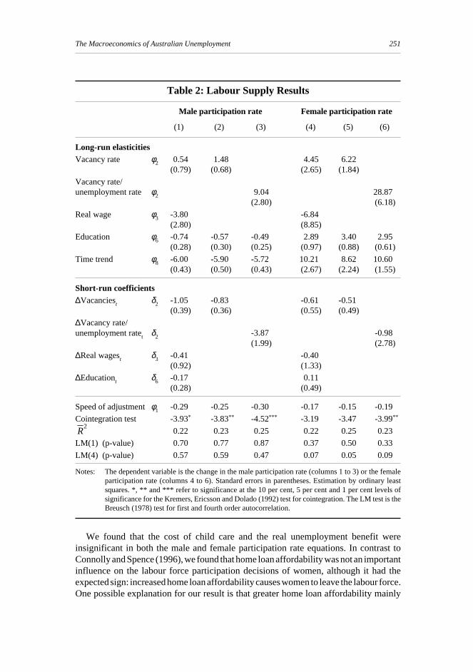
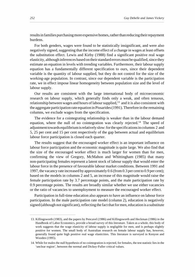
251The Macroeconomics of Australian Unemployment
Table 2: Labour Supply Results
Male participation rate Female participation rate
(1) (2) (3) (4) (5) (6)
Long-run elasticitiesVacancy rate φ2 0.54 1.48 4.45 6.22
(0.79) (0.68) (2.65) (1.84)
Vacancy rate/unemployment rate φ2 9.04 28.87
(2.80) (6.18)
Real wage φ3 -3.80 -6.84(2.80) (8.85)
Education φ6 -0.74 -0.57 -0.49 2.89 3.40 2.95(0.28) (0.30) (0.25) (0.97) (0.88) (0.61)
Time trend φ8 -6.00 -5.90 -5.72 10.21 8.62 10.60(0.43) (0.50) (0.43) (2.67) (2.24) (1.55)
Short-run coefficients∆Vacanciest δ2 -1.05 -0.83 -0.61 -0.51
(0.39) (0.36) (0.55) (0.49)
∆Vacancy rate/unemployment ratet δ2 -3.87 -0.98
(1.99) (2.78)
∆Real wagest δ3 -0.41 -0.40(0.92) (1.33)
∆Educationt δ6 -0.17 0.11(0.28) (0.49)
Speed of adjustmentφ1 -0.29 -0.25 -0.30 -0.17 -0.15 -0.19
Cointegration test -3.93* -3.83** -4.52*** -3.19 -3.47 -3.99**
R2
0.22 0.23 0.25 0.22 0.25 0.23
LM(1) (p-value) 0.70 0.77 0.87 0.37 0.50 0.33
LM(4) (p-value) 0.57 0.59 0.47 0.07 0.05 0.09
Notes: The dependent variable is the change in the male participation rate (columns 1 to 3) or the femaleparticipation rate (columns 4 to 6). Standard errors in parentheses. Estimation by ordinary leastsquares. *, ** and *** refer to significance at the 10 per cent, 5 per cent and 1 per cent levels ofsignificance for the Kremers, Ericsson and Dolado (1992) test for cointegration. The LM test is theBreusch (1978) test for first and fourth order autocorrelation.
We found that the cost of child care and the real unemployment benefit wereinsignificant in both the male and female participation rate equations. In contrast toConnolly and Spence (1996), we found that home loan affordability was not an importantinfluence on the labour force participation decisions of women, although it had theexpected sign: increased home loan affordability causes women to leave the labour force.One possible explanation for our result is that greater home loan affordability mainly
252 Guy Debelle and James Vickery
results in families purchasing more expensive homes, rather than reducing their repaymentburdens.
For both genders, wages were found to be statistically insignificant, and were alsonegatively signed, suggesting that the income effect of a change in wages at least offsetsthe substitution effect. Lewis and Kirby (1988) find a significant positive real wageelasticity, although inferences based on their standard errors must be qualified, since theyestimate an equation in levels with trending variables. Furthermore, their labour supplyequation has a fundamentally different specification to ours, since their dependentvariable is the quantity of labour supplied, but they do not control for the size of theworking-age population. In contrast, since our dependent variable is the participationrate, we in effect impose linear homogeneity between population size and the level oflabour supply.
Our results are consistent with the large international body of microeconomicresearch on labour supply, which generally finds only a weak, and often tenuous,relationship between wages and hours of labour supplied,13 and it is also consistent withthe aggregate participation rate equation in Pissarides (1991). Therefore in the remainingcolumns, we exclude wages from the specification.
The evidence for a cointegrating relationship is weaker than in the labour demandequation, where the null of no cointegration was clearly rejected.14 The speed ofadjustment towards equilibrium is relatively slow: for the specifications in columns 2 and5, 25 per cent and 15 per cent respectively of the gap between actual and equilibriumlabour force participation is closed each quarter.
The results suggest that the encouraged worker effect is an important influence onlabour force participation and the economic magnitude is quite large. We also find thatthe size of the encouraged worker effect is much larger for women than for men,confirming the view of Gregory, McMahon and Whittingham (1985) that manynon-participating females represent a latent stock of labour supply that would enter thelabour force in the presence of favourable labour market conditions. Between 1991 and1997, the vacancy rate increased by approximately 0.6 (from 0.3 per cent to 0.9 per cent);based on the models in columns 2 and 5, an increase of this magnitude would raise thefemale participation rate by 3.7 percentage points, and the male participation rate by0.9 percentage points. The results are broadly similar whether we use either vacanciesor the ratio of vacancies to unemployment to measure the encouraged worker effect.
Participation in full-time education also appears to have an influence on labour forceparticipation. In the male participation rate model (column 2), education is negativelysigned (although not significant), reflecting the fact that for men, education is a substitute
13. Killingsworth (1983), and the papers by Pencavel (1986) and Killingsworth and Heckman (1986) in theHandbook of Labor Economics, provide a broad survey of this literature. Taken as a whole, this body ofwork suggests that the wage elasticity of labour supply is negligible for men, and is perhaps slightlypositive for women. The small body of Australian research on female labour supply has, however,generally found quite high positive real wage elasticities. This literature is surveyed in Kenyon andWooden (1995).
14. While for males the null hypothesis of no cointegration is rejected, for females, the test statistic lies in the‘unclear region’, between the normal and Dickey-Fuller critical values.
253The Macroeconomics of Australian Unemployment
for time which would otherwise have been spent in the labour market.15 In the femalemodel, however, the coefficient on education is positively signed and significant. Oneexplanation of this finding is that education is correlated with unobservable demographicchange variables which are driving the persistent upward trend in the female participationrate. Another explanation is that in contrast to males, education provides an opportunityfor females to gain skills which will allow them to gain employment.
The time trend variable is highly significant in both the male and female participationrate equations, suggesting that demographic and attitudinal changes, which we wereunable to capture explicitly within our modelling framework, have been an importantinfluence on the observed changes in participation rates.
In conclusion, our preferred specification for labour supply includes the encouragedworker effect (measured by the vacancy rate), participation in education and a time trend.
5. Reducing UnemploymentIn this section, we use the model presented in Section 3, and the parameters of the
model estimated in Section 4 to provide some benchmark estimates for the size of thereduction in the level of real wages needed to achieve a permanent reduction in the rateof unemployment. That is, we quantify the expression for the elasticity of unemploymentwith respect to the real wage derived in Equation (12). We also examine the adjustmentof the economy to the lower unemployment rate, and the role that monetary policy canplay in that adjustment.
The model is somewhat stylised but it highlights the main relationships involved.Later in the section, we compare the results obtained with those from two more fullyspecified macroeconomic models of the Australian economy.
We assume that initially the economy is in equilibrium at the current natural rate ofunemployment determined by the equilibrium real wage, itself a function of the existingset of labour market institutions. The research reported in Section 2 suggests that thenatural rate is currently likely to be somewhere between 7 and 7.5 per cent. Over time,the unemployment rate should gradually fall to this level without any change in theexogenous component of the real wage or labour market institutions.
The basic core of the model consists of the labour demand and labour supplyequations. The parameters in the labour demand curve are taken from column 3 ofTable 1, where the real wage elasticity is -0.4 and the output elasticity is 1.09. For thepurposes of the simulation we assume that productivity remains constant. Equivalently,output and productivity could grow at a constant rate with no net effect on employment.
We make two different assumptions about the process for output. Firstly, we assumethat output is invariant to changes in employment; that is, the scale effect is one. This islikely to provide a lower bound on the impact of the wage change. Quandt andRosen (1989) however, provide evidence that the scale effect is one in the United States.
Secondly, we assume that output increases proportionately to labour’s share ofincome, 0.58. That is, a one percentage point increase in employment leads to a
15. While people still participate in the labour force while in the education, the participation rate is lower thanthat for the rest of the population.

254 Guy Debelle and James Vickery
0.58 percentage point increase in output, which amplifies the own price elasticity ofemployment by 2.4 (=1/(1-0.58)). That is, the scale effect is 2.4. This is similar to thelong-run response of output relative to employment in the TRYM model in response toa permanent decline in the natural rate.16
We use the participation rate equations for males and females in columns 2 and 5 inTable 2.17 These are weighted together to give an aggregate participation rate equationby the share of males and females in the working-age population as at December 1997(0.49 and 0.51 respectively). We assume that the participation rate in education remainsconstant at its December 1997 level. We also assume that there are no further trendchanges in participation rates. To the extent that the aggregate participation rate is stillrising through time, the necessary decline in the real wage to achieve a particularunemployment rate would be larger.
The encouraged worker effect is measured using the vacancy rate, so to relate this tomovements in the unemployment rate, we use the Beveridge curve estimated inAppendix A. The employment demand curve is estimated in terms of hours while theBeveridge curve and participation rate equations are estimated in terms of people. Tomap one into the other, we assume that average hours worked remain at their level of end1997.
Starting from an unemployment rate of 7.5 per cent, we consider the impact of areduction in the real wage of two percentage points. The reduction is achieved by adecline in the exogenous component in the wage equation. The exact mechanism bywhich this could be achieved is beyond the scope of this paper, but could include reformsthat permanently changed the balance between insiders and outsiders in wage-setting. Itdoes not imply that only real wages at the lower end of the wage distribution are reduced,but rather that the average real wage in the economy is lowered. Furthermore, given aninflation target of 2 to 3 per cent, this implies that nominal wages do not have to fall toachieve the cut in real wages. Thus issues of nominal wage rigidity can be ignored.
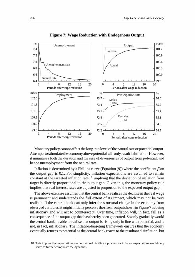
We analyse the sensitivity of these results to different assumptions about the modelparameters, including in particular, the effect of monetary policy on the outcomes. Firstof all, we assume that monetary policy holds the real interest rate at its neutral valuethroughout. Given this assumption, Figure 6 shows the impact on unemployment,employment and male and female participation rates of the two percentage pointreduction in the real wage when the scale effect is 1. Figure 7 shows the results when thescale effect is 2.4.
When the scale effect is 1, there is a fall in the natural rate of unemployment of0.41 percentage points. The adjustment of unemployment to the new lower natural rateis rapid, given the absence of much dynamics in the labour demand and supply equations.The different patterns of adjustment of the male and female participation rates reflect thedifferent sizes of the encouraged worker effects, and the different speed-of-adjustmentparameters. Employment adjusts by a greater proportion (0.8 per cent) than the fall in
16. See Commonwealth Treasury (1996), pp. 34–37. There it is assumed that monetary policy does notaccommodate the increase in real activity but rather lets the price level fall.
17. We ignore the dynamic terms in the two labour supply equations which tended to generate some instabilityin the simulations. This only affects the adjustment process, not the final result.
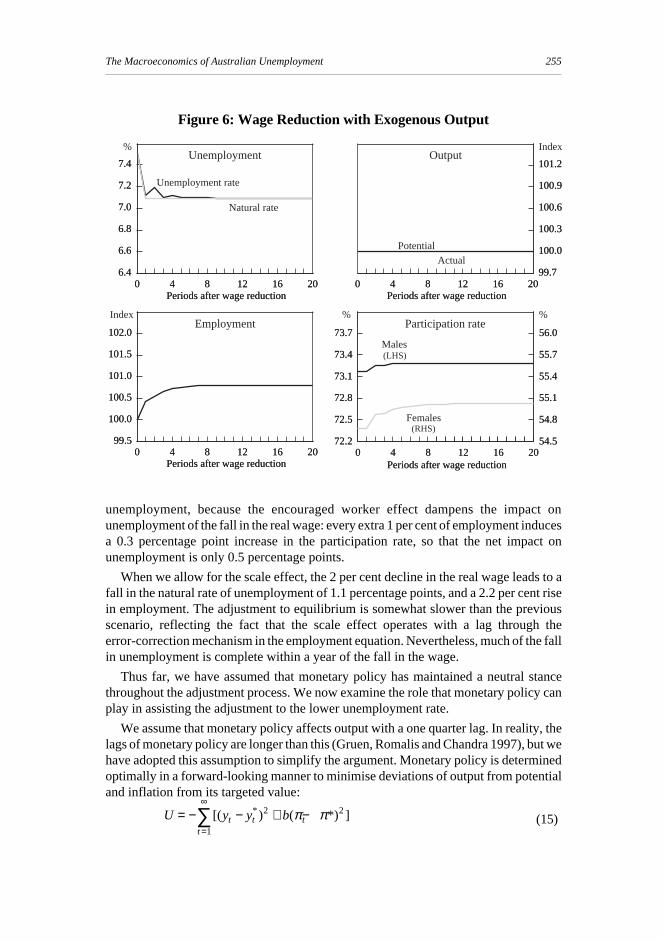
255The Macroeconomics of Australian Unemployment
unemployment, because the encouraged worker effect dampens the impact onunemployment of the fall in the real wage: every extra 1 per cent of employment inducesa 0.3 percentage point increase in the participation rate, so that the net impact onunemployment is only 0.5 percentage points.
When we allow for the scale effect, the 2 per cent decline in the real wage leads to afall in the natural rate of unemployment of 1.1 percentage points, and a 2.2 per cent risein employment. The adjustment to equilibrium is somewhat slower than the previousscenario, reflecting the fact that the scale effect operates with a lag through theerror-correction mechanism in the employment equation. Nevertheless, much of the fallin unemployment is complete within a year of the fall in the wage.
Thus far, we have assumed that monetary policy has maintained a neutral stancethroughout the adjustment process. We now examine the role that monetary policy canplay in assisting the adjustment to the lower unemployment rate.
We assume that monetary policy affects output with a one quarter lag. In reality, thelags of monetary policy are longer than this (Gruen, Romalis and Chandra 1997), but wehave adopted this assumption to simplify the argument. Monetary policy is determinedoptimally in a forward-looking manner to minimise deviations of output from potentialand inflation from its targeted value:
U y y bt t tt
= − − + −=
∞
∑[( ) ( *) ]* 2 2
1
π π (15)
Figure 6: Wage Reduction with Exogenous Output
Unemployment
Unemployment rate
%
0 4 8 12 16 200 4 8 12 16 2099.5
100.0
100.5
101.0
101.5
102.0
99.5
100.0
100.5
101.0
101.5
102.0
Periods after wage reductionPeriods after wage reduction
0 4 8 12 16 200 4 8 12 16 206.4
6.6
6.8
7.0
7.2
7.4
6.4
6.6
6.8
7.0
7.2
7.4
Periods after wage reductionPeriods after wage reduction0 4 8 12 16 200 4 8 12 16 20
99.7
100.0
100.3
100.6
100.9
101.2
99.7
100.0
100.3
100.6
100.9
101.2
Periods after wage reductionPeriods after wage reduction
0 4 8 12 16 200 4 8 12 16 2072.2
72.5
72.8
73.1
73.4
73.7
54.5
54.8
55.1
55.4
55.7
56.0
72.2
72.5
72.8
73.1
73.4
73.7
54.5
54.8
55.1
55.4
55.7
56.0
Periods after wage reductionPeriods after wage reduction
Index % %
IndexOutput
Employment Participation rate
Natural rate
ActualPotential
(RHS)Females
(LHS)Males
256 Guy Debelle and James Vickery
Monetary policy cannot affect the long-run level of the natural rate or potential output.Attempts to stimulate the economy above potential will only result in inflation. However,it minimises both the duration and the size of divergences of output from potential, andhence unemployment from the natural rate.
Inflation is determined by a Phillips curve (Equation (9)) where the coefficient β onthe output gap is 0.1. For simplicity, inflation expectations are assumed to remainconstant at the targeted inflation rate,18 implying that the deviation of inflation fromtarget is directly proportional to the output gap. Given this, the monetary policy ruleimplies that real interest rates are adjusted in proportion to the expected output gap.
The above exercise assumes that the central bank realises the decline in the real wageis permanent and understands the full extent of its impact, which may not be veryrealistic. If the central bank can only infer the structural change in the economy fromobserved variables, it might initially perceive the rise in output shown in Figure 7 as beinginflationary and will act to counteract it. Over time, inflation will, in fact, fall as aconsequence of the output gap that has thereby been generated. So only gradually wouldthe central bank be able to realise that output is rising only in line with potential, and isnot, in fact, inflationary. The inflation-targeting framework ensures that the economyeventually returns to potential as the central bank reacts to the resultant disinflation, but
Figure 7: Wage Reduction with Endogenous Output
Unemployment
Unemployment rate
%
0 4 8 12 16 200 4 8 12 16 2099.5
100.0
100.5
101.0
101.5
102.0
99.5
100.0
100.5
101.0
101.5
102.0
Periods after wage reductionPeriods after wage reduction
0 4 8 12 16 200 4 8 12 16 206.4
6.6
6.8
7.0
7.2
7.4
6.4
6.6
6.8
7.0
7.2
7.4
Periods after wage reductionPeriods after wage reduction0 4 8 12 16 200 4 8 12 16 20
99.7
100.0
100.3
100.6
100.9
101.2
99.7
100.0
100.3
100.6
100.9
101.2
Periods after wage reductionPeriods after wage reduction
0 4 8 12 16 200 4 8 12 16 2072.2
72.5
72.8
73.1
73.4
73.7
54.5
54.8
55.1
55.4
55.7
56.0
72.2
72.5
72.8
73.1
73.4
73.7
54.5
54.8
55.1
55.4
55.7
56.0
Periods after wage reductionPeriods after wage reduction
Index % %
IndexOutput
Employment Participation rate
Natural rate
Actual
Potential
(LHS)Males
(RHS)Females
18. This implies that expectations are not rational. Adding a process for inflation expectations would onlyserve to further complicate the dynamics.
257The Macroeconomics of Australian Unemployment
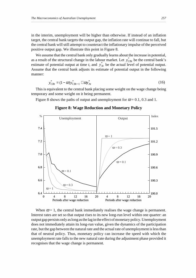
in the interim, unemployment will be higher than otherwise. If instead of an inflationtarget, the central bank targets the output gap, the inflation rate will continue to fall, butthe central bank will still attempt to counteract the inflationary impulse of the perceivedpositive output gap. We illustrate this point in Figure 8.
We assume that the central bank only gradually learns about the increase in potential,as a result of the structural change in the labour market. Let yCBt
* be the central bank’sestimate of potential output at time t, and yAt
* be the actual level of potential output.Assume that the central bank adjusts its estimate of potential output in the followingmanner:
y y yCBt CBt At* * *( )= − +−1 1ω ω (16)
This is equivalent to the central bank placing some weight on the wage change beingtemporary and some weight on it being permanent.
Figure 8 shows the paths of output and unemployment for ω = 0.1, 0.3 and 1.
Figure 8: Wage Reduction and Monetary Policy
UnemploymentIndex%
4 8 12 16 204 8 12 16 20100.0
100.3
100.6
100.9
101.2
101.5
100.0
100.3
100.6
100.9
101.2
101.5
Periods after wage reductionPeriods after wage reduction0 4 8 12 16 200 4 8 12 16 20
6.4
6.6
6.8
7.0
7.2
7.4
6.4
6.6
6.8
7.0
7.2
7.4
Periods after wage reductionPeriods after wage reduction
Output
ω = 0.3
ω = 0.1
ω = 1
ω = 0.1
ω = 0.3
ω = 1
When ω = 1, the central bank immediately realises the wage change is permanent.Interest rates are set so that output rises to its new long-run level within one quarter: anoutput gap persists only as long as the lag in the effect of monetary policy. Unemploymentdoes not immediately attain its long-run value, given the dynamics of the participationrate, but the gap between the natural rate and the actual rate of unemployment is less thanthat of neutral policy. Thus, monetary policy can increase the speed with which theunemployment rate falls to the new natural rate during the adjustment phase provided itrecognises that the wage change is permanent.
258 Guy Debelle and James Vickery
In practice, it will be difficult for the central bank firstly to identify the change, andsecondly to ascertain whether it is permanent or not. We now take account of this fact.When ω is set equal to 0.1, the central bank believes that the chance that the wage changeis permanent is quite small. When the central bank sees stronger output growth, itbelieves that output has risen above potential and acts to counteract that with higherinterest rates, although this is mitigated to some extent by the fact that inflation is fallingbelow its targeted level because, in reality, output is below potential. Unemploymentclearly takes a longer time to reach the lower steady state level. The gap between theactual unemployment rate and the natural rate of unemployment is greater than 0.1percentage points for over three years. In the intermediate case when ω = 0.3, theunemployment rate still falls more slowly than if the central bank believed the wagechange was permanent immediately.
Above we have assumed that the real wage has fallen but the central bank believes itis temporary. If on the other hand, the central bank believes that the wage change ispermanent when in fact it is temporary, it will believe that the level of potential outputhas risen (when in fact it has not) and will therefore loosen policy. This will lead to a risein inflation, which will need to be counteracted by a period of unemployment above thenatural rate.
There are clearly problems of possible misinterpretation in both directions. Inpractice, it is extremely difficult to identify whether such developments in the labourmarket are temporary or permanent, particularly in a period of ongoing structural change.Nevertheless, the results suggest that the central bank can enhance the adjustmentprocess by constantly monitoring and assessing the economy in light of new evidenceabout developments in the labour market. An inflation target can assist this processbecause the focus on the inflation rate will alert the central bank to the possibility ofstructural change when the inflation rate persistently undershoots its forecast value.
Thus far, we have ignored the effect of changes in the capital stock as a result of thechange in the real wage, and the induced increase in employment. The fall in the realwage will cause firms to substitute labour for capital. However, the scale effect willinduce more investment and an expansion of the capital stock. This process is difficultto quantify in the framework used here, however, the Murphy and TRYM modelsexplicitly address this issue (Commonwealth Treasury 1996; Murphy 1992). Bothmodels have a direct link between the natural rate and the real wage, and have a labourmarket structure very similar to the one used here. In terms of the model in Section 3, theprimary difference is that these models incorporate a direct feedback from the capitalstock to the real wage in the medium to long term.
Brooker (1993) examines the effect of a cut in the real wage in both models and findsthat the fall in the real wage initially results in a decline in the capital stock as firmssubstitute towards labour. However, in the longer term the reduction in the real wageincreases the expected return on capital and hence leads to an increase in investment,which in turn leads to a further increase in employment. This process is eventuallycurtailed by a feedback mechanism from the increased employment to a higher realwage. In the long run, the real wage can even rise above its initial value, but the initialdecline is still necessary to stimulate the adjustment. There is still the need for apermanent shift in labour market institutions. The new long-run equilibrium with the
259The Macroeconomics of Australian Unemployment
higher real wage and capital stock is not compatible with the initial institutionalframework.
The two models tend to generate a slightly higher increase in employment as a resultof a decline in the real wage than that presented here, because of the long-run increasein the capital stock. The TRYM model also finds that the lower unemployment ratedecreases the amount of unemployment benefits paid. This then permits the governmentto reduce the tax rate resulting in a rise in after-tax wages which can offset the initialdecrease (Stacey and Downes 1995).
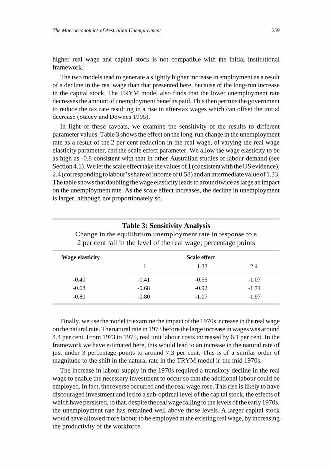
In light of these caveats, we examine the sensitivity of the results to differentparameter values. Table 3 shows the effect on the long-run change in the unemploymentrate as a result of the 2 per cent reduction in the real wage, of varying the real wageelasticity parameter, and the scale effect parameter. We allow the wage elasticity to beas high as -0.8 consistent with that in other Australian studies of labour demand (seeSection 4.1). We let the scale effect take the values of 1 (consistent with the US evidence),2.4 (corresponding to labour’s share of income of 0.58) and an intermediate value of 1.33.The table shows that doubling the wage elasticity leads to around twice as large an impacton the unemployment rate. As the scale effect increases, the decline in unemploymentis larger, although not proportionately so.
Table 3: Sensitivity AnalysisChange in the equilibrium unemployment rate in response to a2 per cent fall in the level of the real wage; percentage points
Wage elasticity Scale effect
1 1.33 2.4
-0.40 -0.41 -0.56 -1.07
-0.68 -0.68 -0.92 -1.71
-0.80 -0.80 -1.07 -1.97
Finally, we use the model to examine the impact of the 1970s increase in the real wageon the natural rate. The natural rate in 1973 before the large increase in wages was around4.4 per cent. From 1973 to 1975, real unit labour costs increased by 6.1 per cent. In theframework we have estimated here, this would lead to an increase in the natural rate ofjust under 3 percentage points to around 7.3 per cent. This is of a similar order ofmagnitude to the shift in the natural rate in the TRYM model in the mid 1970s.
The increase in labour supply in the 1970s required a transitory decline in the realwage to enable the necessary investment to occur so that the additional labour could beemployed. In fact, the reverse occurred and the real wage rose. This rise is likely to havediscouraged investment and led to a sub-optimal level of the capital stock, the effects ofwhich have persisted, so that, despite the real wage falling to the levels of the early 1970s,the unemployment rate has remained well above those levels. A larger capital stockwould have allowed more labour to be employed at the existing real wage, by increasingthe productivity of the workforce.
260 Guy Debelle and James Vickery
6. ConclusionThe primary conclusion of this paper is that the average level of real wages can have
a significant impact on the long-run level of unemployment in the economy. The paperhas suggested that slower growth in real wages of 2 per cent for a year could lead to apermanent reduction in the unemployment rate of around 1 percentage point. The finaldecrease in the unemployment rate may indeed be even larger if there is a long-runincrease in investment and the capital stock as a result of the fall in wage growth.
Estimates of the long-run or natural rate of unemployment suggest that it rose sharplyin the 1970s associated with the rapid rise in labour costs at the time but has sincefluctuated between 6 and 7.5 per cent. Our estimates imply that the wage rise in the 1970smay have increased the natural rate by around 3 percentage points.
Results from our labour demand equation confirm the findings of previous studies thatthe elasticity of employment with respect to output is close to unity. Our estimate for thewage elasticity of employment of -0.4 is lower than empirical work from the 1980s, butis consistent with a range of international evidence and the estimates reported in Dungeyand Pitchford (1998) in this volume. We find clear evidence that labour supply issensitive to the state of the labour market – the ‘encouraged worker effect’. The size ofthis effect is much larger for women than for men. We also find that labour supply isrelatively invariant to real wages.
Monetary policy does not have any impact on the natural rate but can seek to ensurethat the unemployment rate remains as close as possible to the natural rate by avoiding,as far as possible, sharp swings in the business cycle. Maintaining a relatively constantrate of economic growth can reduce the average unemployment rate, although the naturalrate provides a lower bound. Inflation expectations also play a critical role. The fact thatthe unemployment rate has been above the natural rate for most of the 1990s, is in partdue to the slow adjustment of inflation expectations to the lower inflation rate.
Monetary policy can also play a role in the transition process to a lower unemploymentrate in the event of structural change in the labour market. In practice, it is extremelydifficult to identify whether developments in the labour market are temporary orpermanent. However, forward-looking monetary policy that is cognisant of the structuralchange going on in the economy can reduce the amount of excess unemployment duringthe adjustment phase. An inflation-targeting framework for monetary policy is beneficialin this regard by ensuring that monetary policy is forward-looking and becausedevelopments in the labour market are a crucial component of the outlook for inflation.

261The Macroeconomics of Australian Unemployment
Appendix A: The Beveridge CurveIn this Appendix, we estimate a Beveridge curve for Australia and examine whether
changes in the efficiency with which workers are matched with the vacant jobs havecaused the curve to shift over time, in order to indirectly assess whether those factors arelikely to have caused the natural rate to rise over time.
We measure changes in the efficiency of the matching function by: an index ofsectoral dispersion to capture mismatch between skills supplied and demanded(Lilien 1982); the standard deviation of state unemployment rates to measure geographicmismatch; the share of young people in the labour force, as they tend to have a greaterproclivity to move from job to job to find one that suits; and the real level of theunemployment benefit which may affect search intensity.
We estimate the curve using an error-correction specification over the period1979:Q3–1997:Q4. We find that none of the above characteristics of the efficiency of thelabour market are statistically significant. Furthermore, a time trend to capture anyongoing shift in the curve caused by other factors was also insignificant, indicating thatthe Beveridge curve has not shifted over the period. However, Figure 2 suggests that mostof the rise in the natural rate may have occurred in the mid 1970s, which predates thesample period employed here (Harper 1980).
In Table A1, we report our estimate of the Beveridge curve which we use in Section 5.The results confirm the negative relationship between unemployment u and vacanciesvsuggested by Figure 3.
Table A1: Estimate of the Beveridge Curve
∆ ∆ ∆u v u u vt t t t t= − + − −− − −0 16 0 20 0 27 0 09 0 79
0 05 0 04 0 101 1 1. . . . ( . )
( . ) ( . ) ( . )
R2
= 0.65 LM(1) p-value = 0.21 LM(4) p-value = 0.38
Notes: The Kremers, Ericsson and Dolado (1992) test for cointegration has a test statistic of -3.06, whichlies in the indeterminate region between the normal and Dickey-Fuller distributions. Standard errorsare in parentheses.
262 Guy Debelle and James Vickery
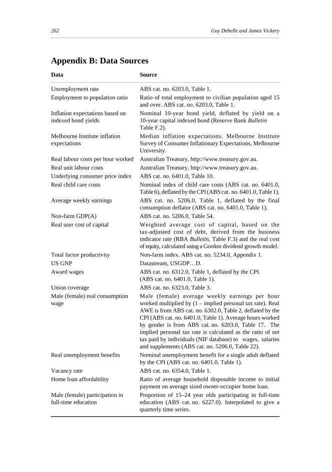
Appendix B: Data Sources
Data Source
Unemployment rate ABS cat. no. 6203.0, Table 1.
Employment to population ratio Ratio of total employment to civilian population aged 15and over. ABS cat. no. 6203.0, Table 1.
Inflation expectations based on Nominal 10-year bond yield, deflated by yield on aindexed bond yields 10-year capital indexed bond (Reserve Bank Bulletin
Table F.2).
Melbourne Institute inflation Median inflation expectations. Melbourne Instituteexpectations Survey of Consumer Inflationary Expectations, Melbourne
University.
Real labour costs per hour worked Australian Treasury, http://www.treasury.gov.au.
Real unit labour costs Australian Treasury, http://www.treasury.gov.au.
Underlying consumer price index ABS cat. no. 6401.0, Table 10.
Real child care costs Nominal index of child care costs (ABS cat. no. 6401.0,Table 6), deflated by the CPI (ABS cat. no. 6401.0, Table 1).
Average weekly earnings ABS cat. no. 5206.0, Table 1, deflated by the finalconsumption deflator (ABS cat. no. 6401.0, Table 1).
Non-farm GDP(A) ABS cat. no. 5206.0, Table 54.
Real user cost of capital Weighted average cost of capital, based on thetax-adjusted cost of debt, derived from the businessindicator rate (RBA Bulletin, Table F.3) and the real costof equity, calculated using a Gordon dividend growth model.
Total factor productivity Non-farm index. ABS cat. no. 5234.0, Appendix 1.
US GNP Datastream, USGDP…D.
Award wages ABS cat. no. 6312.0, Table 1, deflated by the CPI.(ABS cat. no. 6401.0, Table 1).
Union coverage ABS cat. no. 6323.0, Table 3.
Male (female) real consumption Male (female) average weekly earnings per hourwage worked multiplied by (1 – implied personal tax rate). Real
AWE is from ABS cat. no. 6302.0, Table 2, deflated by theCPI (ABS cat. no. 6401.0, Table 1). Average hours workedby gender is from ABS cat. no. 6203.0, Table 17. Theimplied personal tax rate is calculated as the ratio of nettax paid by individuals (NIF database) to wages, salariesand supplements (ABS cat. no. 5206.0, Table 22).
Real unemployment benefits Nominal unemployment benefit for a single adult deflatedby the CPI (ABS cat. no. 6401.0, Table 1).
Vacancy rate ABS cat. no. 6354.0, Table 1.
Home loan affordability Ratio of average household disposable income to initialpayment on average sized owner-occupier home loan.
Male (female) participation in Proportion of 15–24 year olds participating in full-timefull-time education education (ABS cat. no. 6227.0). Interpolated to give a
quarterly time series.
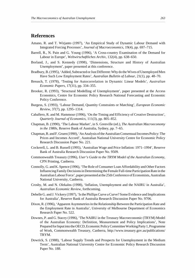
263The Macroeconomics of Australian Unemployment
ReferencesAmano, R. and T. Wirjanto (1997), ‘An Empirical Study of Dynamic Labour Demand with
Integrated Forcing Processes’, Journal of Macroeconomics, 19(4), pp. 697–715.
Barrell, R., N. Pain and G. Young (1996), ‘A Cross-country Examination of the Demand forLabour in Europe’, Weltwirschaftliches Archiv, 132(4), pp. 638–650.
Borland, J., and S. Kennedy (1998), ‘Dimensions, Structure and History of AustralianUnemployment’, paper presented at this conference.
Bradbury, B. (1995), ‘Added, Subtracted or Just Different: Why do the Wives of Unemployed MenHave Such Low Employment Rates’, Australian Bulletin of Labour, 21(1), pp. 48–70.
Breusch, T. (1978), ‘Testing for Autocorrelation in Dynamic Linear Models’, AustralianEconomic Papers, 17(31), pp. 334–355.
Brooker, R. (1993), ‘Structural Modelling of Unemployment’, paper presented at the AccessEconomics, Centre for Economic Policy Research National Forecasting and EconomicPolicy Conference.
Burgess, S. (1993), ‘Labour Demand, Quantity Constraints or Matching’, European EconomicReview, 37(7), pp. 1295–1314.
Caballero, R. and M. Hammour (1996), ‘On the Timing and Efficiency of Creative Destruction’,Quarterly Journal of Economics, 111(3), pp. 805–852.
Chapman, B. (1990), ‘The Labour Market’, in S. Grenville (ed.), The Australian Macroeconomyin the 1980s, Reserve Bank of Australia, Sydney, pp. 7–65.
Chapman, B. and F. Gruen (1990), ‘An Analysis of the Australian Consensual Incomes Policy: ThePrices and Incomes Accord’, Australian National University Centre for Economic PolicyResearch Discussion Paper No. 221.
Cockerell, L. and B. Russell (1995), ‘Australian Wage and Price Inflation: 1971–1994’, ReserveBank of Australia Research Discussion Paper No. 9509.
Commonwealth Treasury (1996), User’s Guide to the TRYM Model of the Australian Economy,CPN Printing, Canberra.
Connolly, G. and K. Spence (1996), ‘The Role of Consumer Loan Affordability and Other FactorsInfluencing Family Decisions in Determining the Female Full-time Participation Rate in theAustralian Labour Force’, paper presented at the 25th Conference of Economists, AustralianNational University, Canberra.
Crosby, M. and N. Olekalns (1998), ‘Inflation, Unemployment and the NAIRU in Australia’,Australian Economic Review, forthcoming.
Debelle G. and J. Vickery (1997), ‘Is the Phillips Curve a Curve? Some Evidence and Implicationsfor Australia’, Reserve Bank of Australia Research Discussion Paper No. 9706.
Dixon, R. (1996), ‘Apparent Asymmetries in the Relationship Between the Participation Rate andthe Employment Rate in Australia’, University of Melbourne Department of EconomicsResearch Paper No. 522.
Downes, P. and G. Stacey (1996), ‘The NAIRU in the Treasury Macroeconomic (TRYM) Modelof the Australian Economy: Definition, Measurement and Policy Implications’, NotePrepared for Input into the OECD, Economic Policy Committee Working Party 1, Programmeof Work, Commonwealth Treasury, Canberra, http://www.treasury.gov.au/publications/TRYM.
Dowrick, S. (1988), ‘Labour Supply Trends and Prospects for Unemployment in the MediumTerm’, Australian National University Centre for Economic Policy Research DiscussionPaper No. 188.
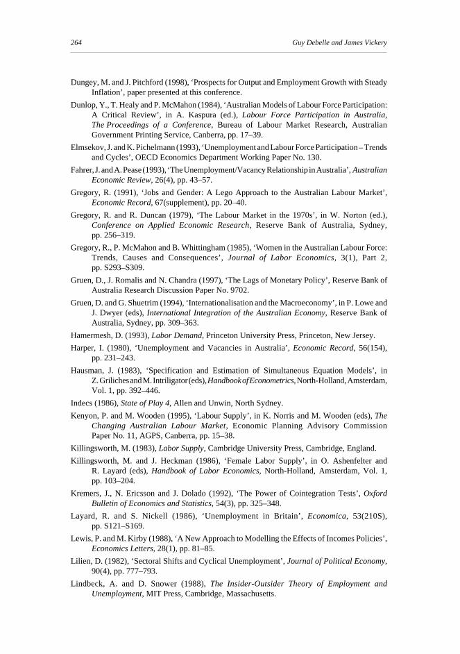
264 Guy Debelle and James Vickery
Dungey, M. and J. Pitchford (1998), ‘Prospects for Output and Employment Growth with SteadyInflation’, paper presented at this conference.
Dunlop, Y., T. Healy and P. McMahon (1984), ‘Australian Models of Labour Force Participation:A Critical Review’, in A. Kaspura (ed.), Labour Force Participation in Australia,The Proceedings of a Conference, Bureau of Labour Market Research, AustralianGovernment Printing Service, Canberra, pp. 17–39.
Elmsekov, J. and K. Pichelmann (1993), ‘Unemployment and Labour Force Participation – Trendsand Cycles’, OECD Economics Department Working Paper No. 130.
Fahrer, J. and A. Pease (1993), ‘The Unemployment/Vacancy Relationship in Australia’, AustralianEconomic Review, 26(4), pp. 43–57.
Gregory, R. (1991), ‘Jobs and Gender: A Lego Approach to the Australian Labour Market’,Economic Record, 67(supplement), pp. 20–40.
Gregory, R. and R. Duncan (1979), ‘The Labour Market in the 1970s’, in W. Norton (ed.),Conference on Applied Economic Research, Reserve Bank of Australia, Sydney,pp. 256–319.
Gregory, R., P. McMahon and B. Whittingham (1985), ‘Women in the Australian Labour Force:Trends, Causes and Consequences’, Journal of Labor Economics, 3(1), Part 2,pp. S293–S309.
Gruen, D., J. Romalis and N. Chandra (1997), ‘The Lags of Monetary Policy’, Reserve Bank ofAustralia Research Discussion Paper No. 9702.
Gruen, D. and G. Shuetrim (1994), ‘Internationalisation and the Macroeconomy’, in P. Lowe andJ. Dwyer (eds), International Integration of the Australian Economy, Reserve Bank ofAustralia, Sydney, pp. 309–363.
Hamermesh, D. (1993), Labor Demand, Princeton University Press, Princeton, New Jersey.
Harper, I. (1980), ‘Unemployment and Vacancies in Australia’, Economic Record, 56(154),pp. 231–243.
Hausman, J. (1983), ‘Specification and Estimation of Simultaneous Equation Models’, inZ. Griliches and M. Intriligator (eds), Handbook of Econometrics, North-Holland, Amsterdam,Vol. 1, pp. 392–446.
Indecs (1986), State of Play 4, Allen and Unwin, North Sydney.
Kenyon, P. and M. Wooden (1995), ‘Labour Supply’, in K. Norris and M. Wooden (eds), TheChanging Australian Labour Market, Economic Planning Advisory CommissionPaper No. 11, AGPS, Canberra, pp. 15–38.
Killingsworth, M. (1983), Labor Supply, Cambridge University Press, Cambridge, England.
Killingsworth, M. and J. Heckman (1986), ‘Female Labor Supply’, in O. Ashenfelter andR. Layard (eds), Handbook of Labor Economics, North-Holland, Amsterdam, Vol. 1,pp. 103–204.
Kremers, J., N. Ericsson and J. Dolado (1992), ‘The Power of Cointegration Tests’, OxfordBulletin of Economics and Statistics, 54(3), pp. 325–348.
Layard, R. and S. Nickell (1986), ‘Unemployment in Britain’, Economica, 53(210S),pp. S121–S169.
Lewis, P. and M. Kirby (1988), ‘A New Approach to Modelling the Effects of Incomes Policies’,Economics Letters, 28(1), pp. 81–85.
Lilien, D. (1982), ‘Sectoral Shifts and Cyclical Unemployment’, Journal of Political Economy,90(4), pp. 777–793.
Lindbeck, A. and D. Snower (1988), The Insider-Outsider Theory of Employment andUnemployment, MIT Press, Cambridge, Massachusetts.
265The Macroeconomics of Australian Unemployment
Macfarlane, I. (1997), ‘Monetary Policy, Growth and Unemployment’, Reserve Bank of AustraliaBulletin, June, pp. 1–8.
Murphy, C. (1992), Access Economics Murphy Model Manual Version 2.1, The Model in Detail,Access Economics Pty Ltd, Canberra.
OECD (1996), OECD Economic Surveys, Australia, OECD, Paris.
Parkin, M. (1973), ‘The Short-run and Long-run Trade-offs between Inflation and Unemploymentin Australia’, Australian Economic Papers, 12(21), pp. 127–144.
Pencavel, J. (1986), ‘Labor Supply of Men: A Survey’, in O. Ashenfelter and R. Layard (eds),Handbook of Labour Economics, North-Holland, Amsterdam, Vol. 1, pp. 2–102.
Pissarides, C. (1991), ‘Real Wages and Unemployment in Australia’, Economica, 58(229),pp. 35–55.
Quandt, R. and H. Rosen (1989), ‘Endogenous Output in an Aggregate Model of the LaborMarket’, Review of Economics and Statistics, 71(3), pp. 394–400.
Russell, B. and W. Tease (1991), ‘Employment, Output and Real Wages’, Economic Record,67(196), pp. 34–45.
Sargent, T. (1978), ‘Estimation of Dynamic Labor Demand Schedules under Rational Expectations’,Journal of Political Economy, 86(6), pp. 1009–1044.
Shapiro, C. and J. Stiglitz (1984), ‘Equilibrium Unemployment as a Worker-Discipline Device’,American Economic Review, 74(2), pp. 433–444.
Simes, R. and C. Richardson (1987), ‘Wage Determination in Australia’, Economic Record,63(181), pp. 144–155.
Stacey, G. and P. Downes (1995), ‘Wage Determination and the Labour Market in the TreasuryMacroeconomic (TRYM) Model’, paper presented at the 24th Conference of Economists,Adelaide.
Watts, M. and W. Mitchell (1990), ‘Australian Wage Inflation: Real Wage Resistance, Hysteresisand Incomes Policy: 1968(3)–1988(3)’, The Manchester School, 58(2), pp. 142–164.