THE MG MODEL FOR THE ESTIMATION OF PEAK FLOOD FLOWS, application to French rivers

THE MG MODEL FOR THE ESTIMATION OF PEAK FLOOD FLOWS

Majone Ugo(1), Tomirotti Massimo(2) , Galimberti Giacomo(3)

(1)DIIAR, Polytechnic of Milan, 32 L. Da Vinci Square, 20132 Milan, Italy,

phone: +39 02 23996210; fax: +39 02 23996298; e-mail: [email protected] (2)DICATA, University of Brescia, 43 Branze Street, 25123 Brescia, Italy

phone: +39 030 3711290; fax: +39 030 3711312; e-mail: [email protected] (3)Studio Maione Ingegneri Associati, 7 Inama Street, 20133 Milan, Italy

phone: +39 02 70120918; fax: +39 02 70120923; e-mail: [email protected]

ABSTRACT The present paper describes the results of a regional analysis of peak flood flows that has

been carried out on the basis of the data recorded in more than 8500 gauging stations belonging to different geographical areas of Europe, North America, Oceania and to other sites of Africa, Asia and South America.

The regionalization procedure is based on definition of a dimensionless variable Y (obtained by a suitable standardization of the peak discharge) whose probability distribution can be assumed constant for all the considered sites.

The probabilistic model (MG model) obtained by interpolation of the empirical non exceedance frequencies of the maximum values of Y observed at each gauged site gives the probability distribution of peak discharges for return periods ranging from 30-50 years (nearly equal to the average length of the considered series) up to about 4000 years. With respect to other probability distributions currently used for the same purpose, the MG model provides a better interpolation of the empirical non exceedance frequencies of peak discharges, especially for long return periods. The validation has been performed on nearly 1400 French gauging stations and it turned out that the empirical frequency distribution obtained for French rivers are in good agreement with the MG model.

The value Y=7 – corresponding to about a 4000 year return period – is the upper bound for which the interpolation of the frequency distribution of Y provided by the MG model can be considered reliable; moreover, the value Y=9 is the absolute maximum of the empirical values of the standardized variable with reference to the 8500 considered gauging stations. These values can be assumed both to define the “predictability bound” of flood events and to estimate the design peak discharges in cases of particularly high risk levels.

Keywords: peak flood flows, regional estimation, unpredictable events, maximum probable flood discharge 1 INTRODUCTION

The estimation of peak discharges to be assumed for flood protection planning is usually performed on the basis of return periods much longer with respect to the historical series that are usually available. For instance, in Italy the above mentioned return periods range from 100 to 500 years. Another typical example is the design of dam spillways, that in Italy but also in other countries is usually performed on the basis of a 1000 years return period flood.

The reliability of such estimations, referring to frequency values much smaller than the observed ones, is questionable.

Moreover, in the judicial for the assessment of the liabilities regarding the damage caused by floods, inundations and every other disaster resulting from the overflow of rivers, it is required by judicial authorities to establish whether the event causing the damage has to be considered exceptional or unpredictable according to the meaning of these terms in common speech. In fact, it appears that the damage caused by events that can be defined as absolutely

unpredictable might not be charged to any subject, private or public as it may be. A possible way to face this problem is the definition of a limit value of peak discharge

that can be assumed as an upper bound beyond which the estimates loose their significance, due to the lack of exceeding data. Due to the limited size of the historical series, the search for this “predictability bound” requires both the analysis of flood flows recorded at as many gauging stations as possible and the formulation of a suitable methodology to render homogeneous data referring to natural systems that can vary from each other with respect to dimensions, climate, and physical characteristics1.

The same strategy can be used to render more reliable the estimates of high return period quantiles of peak flows needed for flood protection planning.

To this purpose, in previous papers the authors introduced a new probabilistic model – named the MG model – particularly suitable for the estimation of peak flood discharges corresponding to very high return periods. The formulation of the MG model is based on the definition of a standardized variable whose probability distribution can be assumed constant for all sites inside the considered regions. Moreover, the maximum observed value of the standardized variable was adopted to define the above mentioned limit values of peak discharges.

The methodology was initially applied to Italian river catchments (Maione, 1997; Beretta et al., 2001; Maione, 2002) and then to historical series of annual maximum peak flood discharges of 7300 gauging stations distributed over different regions of the Earth: Italy, Switzerland, Great Britain, USA and also Ethiopia and Peru (Majone & Tomirotti, 2004). More recently, the authors extended the analysis considering the annual maximum peak flood flows recorded in more than 8500 gauging stations belonging to different geographical areas of Europe (Italy, Switzerland, Austria, Great Britain, Portugal), North America (USA, Canada), Oceania (Australia) and to other sites of Africa, Asia and South America (Majone et al., 2007). This paper presents the last results of the research, including model validation on another independent data set referring to nearly 1400 French gauging stations, extracted from the “Banque Nationale de Données pour l'Hydrométrie et l’Hydrologie” maintained by the Ministère de l'Écologie, du Développement et de l'Aménagement Durables. These data have been used to test the MG model and they are not included in the data set used to develop the model.

The results of the analysis confirm the general validity of the MG model and of the criteria used to define the predictability bound of flood events.

2 REGIONAL MODELS

As mentioned above, the characterization of exceptional flood events requires the estimation of peak discharges of return periods much higher than the lengths of the historical series of annual maximum peak flood flows that are usually available; for instance, the average length of the large number of series considered in this studies does not exceed 30-40 years (as confirmed by Tab. 1 of the next section).

A deep analysis of the difficulties arising in these kinds of extrapolations is made by Klemeš (2000a-b). In particular, the author characterizes the high degree of uncertainty of the last points of the empirical frequency curves obtained from random samples; due to this uncertainty, not much variable with sample size, the extrapolated tail of the frequency distribution does not have much credibility.

To make more significant the estimates of high return period quantiles of peak flows and also to allow to treat the case of ungauged sites, regional estimation methods are commonly used; the latter are based on space interpolation and extrapolation techniques of the available 1 This kind of approach was adopted by Fuller (1914) and, in Italy, by Tonini (1939) on the basis of the hydrologic knowledge of that time.

hydrological data. The motivation of regional models is linked to the consideration that if the analysis of the

flood events for a given river site takes into account only the data recorded in the past at the same site it is not very likely that the sample of available data contains some exceptional values, and even if such values have occurred, their statistical interpretation is a difficult task due to the limited size of the samples that are usually available. On the contrary, if the analysis extends (by means of suitable homogeneization criteria) to a large number of independent historical series referring to different rivers it is much more likely that several exceptional values will be encountered. It is presumed that more significant results will be obtained from this kind of analysis.

It is well known that regionalization models based on the “index flood” method assume that it is possible to identify compact and sufficiently large areas that are homogeneous with regard to the characteristics influencing flood formation processes (morphology, geo-lithology, land use, pluviometry, etc.) and include a large number of gauged sites. The key hypothesis is that this hydrologic homogeneity, which is actually defined only in qualitative terms, implies a well-defined statistical behaviour of peak flood discharges for the rivers inside the homogeneous region. In particular, it is assumed that the probability distribution of the standardized variable Q*=Q/µ(Q) – obtained by normalization of the annual maximum peak discharge with respect to the average of the population – is the same for all the river sites inside the homogeneous region. Tthis implies the equality of the moments of every order of Q*. Anyway, if all the series of Q* have an identical average (equal to unity), the same does not hold for the higher order moments and in particular for the coefficient of variation CV(Q) and for the coefficient of skewness γ(Q), if the analysis is limited to second and third order moments; in fact, their sample values often change in a very wide range also inside the homogeneous regions.

So, since the variability of the moments implies the variability of the parameters of the probability distribution of Q*, the size of the error deriving from these models could be very large (e.g. Majone & Tomirotti, 2005).

3 THE MG MODEL

To overcome the previously mentioned difficulties, parametric methods can be used instead of index flood ones. In fact, the former account also for the variability of higher order normalized moments by assuming a unique multi-parameter form of the probability distribution for the peak flood discharge and the regional estimation is achieved by calibrating regression formulas for the parameters in dependence on geomorphoclimatic characteristics of the river basins.

The MG model has been introduced for these kinds of analysis (Maione, 1997; Beretta et al., 2001; Majone & Tomirotti, 2005). In this paper the validity of the model has been extended considering the above mentioned 8500 historical series of annual maximum peak discharges observed at gauging stations belonging to different geographical areas of Europe (Italy, Switzerland, Austria, Great Britain, Portugal), North America (USA, Canada), Oceania (Australia) and to other sites of Africa, Asia and South America. The location of the gauging stations considered in the analysis is shown in Figure 1.

Since the attention is focused on the characterization of high return period quantiles, the MG model has been calibrated on the basis of the maximum values Qmax of the historical series. This choice allows to make more recognizable eventual trends of the data, that otherwise would be masked by the presence of a great amount of peak values characterized by very different (and smaller) return periods.

The selected data, after standardization with respect to the averages of the series are plotted in the (CV, Q/µ) plane in Figure 2a, which shows that the observations can be

interpolated by a concave curve defined by the simple equation Q/µ=1+aCVb with exponent b appreciably greater than unity (as would be the case for a Gumbel distribution) and equal to 1.33.

#S#S

#S#S#S#S

#S#S#S#S#S#S #S#S#S#S#S#S#S#S#S

#S#S#S#S#S#S

#S#S#S#S#S#S#S#S#S#S#S#S#S#S#S#S#S#S#S#S#S#S

#S#S#S#S

#S#S#S#S#S#S#S#S#S#S#S#S#S#S#S#S#S#S#S#S#S#S#S#S#S#S#S#S#S#S#S#S#S#S#S#S#S#S#S#S#S#S#S#S#S#S#S#S#S#S#S#S#S#S#S#S#S#S#S#S#S#S#S#S#S#S#S#S#S#S#S#S#S

#S #S#S#S#S#S#S#S#S#S#S#S

#S#S#S#S#S#S#S#S#S#S#S#S#S#S#S#S#S#S#S#S#S#S#S#S#S#S#S

#S#S#S #S#S#S#S#S#S


#S#S#S#S

#S#S#S#S#S#S#S#S#S#S#S#S#S#S#S#S#S#S#S#S#S#S#S#S#S#S#S

#S#S#S#S#S#S#S#S#S#S#S#S#S#S#S#S#S#S#S#S#S#S#S

#S#S#S#S#S#S#S#S#S#S#S#S#S#S#S#S#S#S

#S#S#S#S#S #S#S#S#S#S#S#S#S#S#S#S#S#S#S#S#S#S#S#S#S#S#S#S

#S#S#S #S#S#S#S#S#S#S#S#S#S#S#S#S#S#S#S#S#S#S#S#S#S #S#S#S#S#S#S#S#S#S#S#S#S#S#S#S#S #S#S#S#S#S#S#S#S#S#S#S#S#S#S

#S#S#S#S#S#S#S#S#S#S#S#S#S#S#S#S#S#S#S#S#S

#S#S#S#S#S#S#S#S#S#S#S#S#S#S#S#S#S#S#S#S#S#S#S#S#S#S#S#S#S

#S#S#S#S#S#S#S #S#S#S#S#S#S#S#S#S#S#S#S#S#S#S#S#S#S#S#S#S

#S#S#S#S#S#S#S#S#S#S#S#S#S#S#S#S


#S#S#S#S#S#S#S#S


#S#S#S#S#S#S#S#S#S#S#S#S#S#S#S#S#S#S#S#S#S#S#S#S#S

#S#S#S#S#S#S#S#S#S#S#S

#S#S#S#S #S#S#S

#S #S#S#S#S

#S

#S#S#S#S #S#S#S#S#S#S#S#S#S#S#S#S#S#S#S#S#S#S#S#S#S#S#S #S#S#S#S#S#S#S#S#S#S#S#S#S #S#S#S#S#S#S#S#S#S#S#S#S

#S#S

#S#S#S#S#S#S#S#S#S#S#S#S#S#S#S#S#S

#S#S#S#S#S#S#S#S#S#S#S#S

#S #S#S

#S#S#S#S#S#S#S#S

#S #S#S#S

#S#S#S#S#S #S#S #S#S#S#S#S #S#S#S

#S

#S

#S#S#S#S#S#S#S#S#S#S#S#S#S#S

#S#S#S#S#S#S#S#S#S#S#S#S#S#S#S#S#S#S#S#S#S#S#S#S#S#S#S#S#S#S#S#S#S#S#S#S#S #S#S#S#S#S#S#S#S#S#S#S#S#S#S#S#S#S#S#S#S#S#S#S#S#S#S#S#S

#S#S#S#S#S#S#S#S#S#S#S#S#S#S#S#S#S#S#S#S#S#S#S#S#S#S#S#S#S#S#S#S

#S#S#S#S#S#S#S#S#S#S#S#S#S#S#S#S#S#S#S#S#S#S#S #S#S#S#S#S#S#S#S#S#S#S#S#S#S#S#S#S#S#S#S#S#S#S#S#S

#S#S #S#S#S#S#S#S#S#S#S#S#S#S#S#S#S#S#S#S#S#S#S#S#S#S#S#S#S#S#S#S#S

#S#S#S #S#S#S#S#S#S#S#S#S#S#S#S#S#S#S#S#S#S#S#S#S#S#S#S#S#S#S#S#S#S#S#S#S#S#S#S#S#S#S


#S#S#S#S#S#S#S#S#S#S#S#S#S#S#S#S#S#S#S#S#S#S#S#S#S#S#S#S#S#S#S#S#S #S#S#S#S#S#S#S#S#S#S#S#S#S#S#S#S#S#S#S#S#S#S#S#S #S#S#S#S#S

#S#S#S#S#S#S#S#S#S#S#S#S#S#S#S#S#S#S#S#S#S#S#S#S#S#S#S#S#S#S#S#S#S #S#S#S#S#S #S#S#S#S#S#S#S#S#S#S#S#S#S#S#S#S #S#S#S#S#S#S#S#S#S#S#S#S#S#S#S#S#S#S#S#S#S#S#S#S#S#S#S#S#S#S#S#S#S#S#S#S#S#S#S#S#S#S#S#S#S

(X (X

(X

(X

(X(X

(X(X(X(X(X(X(X(X(X(X

(X

(X

(X

(X

(X(X(X(X

(X(X

(X(X(X (X

(X

(X (X(X(X(X(X(X

(X(X (X(X(X (X(X(X(X(X(X(X(X(X(X(X (X(X(X(X (X(X(X(X(X (X(X(X(X

(X

(X

(X(X(X(X (X

(X(X

(X(X(X(X

(X

(X

(X

(X(X(X(X(X

(X(X(X(X(X(X(X

(X(X(X(X(X

(X(X(X(X(X(X(X(X

(X(X(X(X(X(X

(X(X (X

(X(X(X(X(X(X(X

(X(X(X(X(X

(X(X (X

(X(X (X

(X(X(X(X(X(X(X

(X(X(X(X (X

(X(X(X

#S#S#S#S#S#S#S#S#S#S#S#S#S#S#S#S#S#S#S#S#S#S#S#S#S#S#S#S#S#S#S#S#S#S#S#S#S#S#S#S#S#S#S#S#S#S#S#S#S#S#S#S#S#S#S#S#S#S#S#S#S#S#S#S#S#S#S#S#S#S#S#S#S#S#S#S#S#S#S#S#S#S#S#S#S#S#S#S#S#S#S#S#S#S#S#S#S#S#S#S#S#S#S#S#S#S#S#S#S#S#S#S#S#S#S#S#S#S#S#S#S#S#S#S#S#S#S#S#S#S#S#S#S#S#S#S#S#S#S#S#S#S#S#S#S#S#S#S#S#S#S#S#S#S#S#S#S#S#S#S#S#S#S#S#S#S#S#S#S#S#S#S#S

#S#S#S#S#S#S#S#S#S#S#S#S#S#S#S#S#S#S#S#S#S#S#S#S#S#S#S#S#S#S#S#S#S#S#S#S#S#S#S#S#S#S#S#S#S#S#S#S#S#S#S#S#S#S#S#S#S#S#S#S#S#S#S#S#S#S#S#S#S#S#S#S#S#S#S#S#S#S#S#S#S#S#S#S#S#S#S#S#S#S#S#S#S#S#S#S#S#S#S#S#S#S#S#S#S#S#S#S#S#S#S#S#S#S#S#S#S#S#S#S#S#S#S#S#S#S#S#S#S#S#S#S#S#S#S#S#S#S#S#S#S#S#S#S#S#S#S#S#S#S#S#S#S#S#S#S#S#S#S#S#S#S#S#S#S#S#S#S#S#S#S#S#S#S#S#S#S#S#S#S#S#S#S#S#S#S#S#S#S#S#S#S#S#S#S#S#S#S#S#S#S#S#S#S#S#S#S#S#S#S#S#S#S#S#S#S#S#S#S#S#S#S#S#S#S#S#S#S#S#S#S#S#S#S#S#S#S#S#S#S#S#S#S#S#S#S#S#S#S#S#S#S#S#S#S#S#S#S#S#S#S#S#S#S#S#S#S#S#S#S#S#S#S#S#S#S#S#S#S#S#S#S#S#S#S#S#S#S#S#S#S#S#S#S#S#S#S#S#S#S#S#S#S#S#S#S#S#S#S#S#S#S#S#S#S#S#S#S#S#S#S#S#S#S#S#S#S#S#S#S#S#S#S#S#S#S#S#S#S#S#S#S#S#S#S#S#S#S#S#S#S#S#S#S#S#S#S#S#S#S#S#S#S#S#S#S#S#S#S#S#S#S#S#S#S#S#S#S#S#S#S#S#S#S#S#S#S#S#S#S#S#S#S#S#S#S#S#S#S#S#S#S#S#S#S#S#S#S#S#S#S#S#S#S#S#S#S#S#S#S#S#S#S#S#S#S#S#S#S#S#S#S#S#S#S#S#S#S#S#S#S#S#S#S#S#S#S#S#S#S#S#S#S#S#S#S#S#S#S#S#S#S#S#S#S#S#S#S#S#S#S#S#S#S#S#S#S#S#S#S#S#S#S#S#S#S#S#S#S#S#S#S#S#S#S#S#S#S#S#S#S#S#S#S#S#S#S#S#S#S#S#S#S#S#S#S#S#S#S#S#S#S#S#S#S#S#S#S#S#S#S#S#S#S#S#S#S#S#S#S#S#S#S#S#S#S#S#S#S#S#S#S#S#S#S#S#S#S#S#S#S#S#S#S#S#S#S#S#S#S#S#S#S#S#S#S#S#S#S#S#S#S#S#S#S#S#S#S#S#S#S#S#S#S#S#S#S#S#S#S#S#S#S#S#S#S#S#S

#S#S#S#S#S#S#S#S#S#S#S#S#S#S#S#S#S#S#S#S#S#S#S#S#S#S#S#S#S#S#S#S#S#S#S#S#S#S#S#S#S#S#S#S#S#S#S#S#S#S#S#S#S#S#S#S#S#S#S#S#S#S#S#S#S#S#S#S#S#S#S#S#S#S#S#S#S#S#S#S#S#S#S#S#S#S#S#S#S#S#S#S#S#S#S#S#S#S#S#S#S#S#S#S#S#S#S#S#S#S#S#S#S#S#S#S#S#S#S#S#S#S#S#S#S#S#S#S#S#S#S#S#S#S#S#S#S#S#S#S#S#S#S#S#S#S#S#S#S#S#S#S#S#S#S#S#S#S#S#S#S#S#S#S#S#S#S#S#S#S#S#S#S#S#S#S#S#S#S#S#S#S#S#S#S#S#S#S#S#S#S#S#S#S#S#S#S#S#S#S#S#S#S#S#S#S#S#S#S#S#S#S#S#S#S#S#S#S#S#S#S#S#S#S#S#S#S#S#S#S#S#S#S#S#S#S#S#S#S#S#S#S#S#S#S#S#S#S#S#S#S#S#S#S#S#S#S#S#S#S#S#S#S#S#S#S#S#S#S#S#S#S#S#S#S#S#S#S#S#S#S#S#S#S#S#S#S#S#S#S#S#S#S#S#S#S#S#S#S#S#S#S#S#S#S#S#S#S#S#S#S#S#S#S#S#S#S#S#S#S#S#S#S#S#S#S#S#S#S#S#S#S#S#S#S#S#S#S#S#S#S#S#S#S#S#S#S#S#S#S#S#S#S#S#S#S#S#S#S#S#S#S#S#S#S#S#S#S#S#S#S#S#S#S#S#S#S#S

#S#S#S#S#S#S#S#S#S#S#S#S#S#S#S#S#S#S#S#S#S#S#S#S#S#S#S#S#S#S#S#S#S#S#S#S#S#S#S#S#S#S#S#S#S#S#S#S#S#S#S#S#S#S#S#S#S#S#S#S#S#S#S#S#S#S#S#S#S#S#S#S#S#S#S#S#S#S#S#S#S#S#S#S#S#S#S#S#S#S#S#S#S#S#S#S#S#S#S#S#S#S#S#S#S#S#S#S#S#S#S#S#S#S#S#S#S#S#S#S#S#S#S#S#S#S#S#S#S#S#S#S#S#S#S#S#S#S#S#S#S#S#S#S#S#S#S#S#S#S#S#S#S#S#S#S#S#S#S#S#S#S#S#S#S#S#S#S#S#S#S#S#S#S#S#S#S#S#S#S#S#S#S#S#S#S#S#S#S#S#S#S#S#S

#S#S#S#S#S#S#S#S#S#S#S#S#S#S#S#S#S#S#S#S#S#S#S#S#S#S#S#S#S#S#S#S#S#S#S#S#S#S#S#S#S#S#S#S#S#S#S#S#S#S#S#S#S#S#S#S#S#S#S#S#S#S#S#S#S#S#S#S#S#S#S#S#S#S#S#S#S#S#S#S#S#S#S#S#S#S#S#S#S#S#S#S#S#S#S#S#S#S#S#S#S#S#S#S#S#S#S#S#S#S#S#S#S#S#S#S#S#S#S#S#S#S#S#S#S#S#S#S#S#S#S#S#S#S#S#S#S#S#S#S#S#S#S#S#S#S#S#S#S#S#S#S#S#S#S#S#S#S#S#S#S#S

#S#S#S#S#S#S#S#S#S#S#S#S#S#S#S#S#S#S#S#S#S#S#S#S#S#S#S#S#S#S#S#S#S#S#S#S#S#S#S#S#S#S#S#S#S#S#S#S#S#S#S#S#S#S#S#S#S#S#S#S#S#S#S#S#S#S#S#S#S#S#S#S#S#S#S#S#S#S#S#S#S#S#S#S#S#S#S#S#S#S#S#S#S#S#S#S#S#S#S#S#S#S#S#S#S#S#S#S#S#S#S#S#S#S#S#S#S#S#S#S#S#S#S#S#S#S#S#S#S#S#S#S#S#S#S#S#S#S#S#S#S#S#S#S#S#S#S#S#S#S#S#S#S#S#S#S#S#S#S#S#S#S#S#S#S#S#S#S#S#S#S#S#S#S#S#S#S#S#S#S#S#S#S#S#S#S#S#S#S

#S#S#S#S#S#S#S#S#S#S#S#S#S#S#S#S#S#S#S#S#S#S#S#S#S#S#S#S#S#S#S#S#S#S#S#S#S#S#S#S#S#S#S#S#S#S#S#S#S#S#S#S#S#S#S#S#S#S#S#S#S#S#S#S#S#S#S#S#S#S#S#S#S#S#S

#S#S#S#S#S#S#S#S#S#S#S#S#S#S#S#S#S#S#S#S#S#S#S#S#S#S#S#S#S#S#S#S#S#S#S#S#S#S#S#S#S#S#S#S#S#S#S#S#S#S#S#S#S#S#S#S#S#S#S#S#S#S#S#S#S#S#S#S#S#S#S#S#S#S#S#S#S#S#S#S#S#S#S#S#S#S#S#S#S#S#S#S#S#S#S#S#S#S#S#S#S#S#S#S#S#S#S#S#S#S#S#S#S#S#S#S#S#S#S#S#S#S#S#S#S#S#S#S #S#S#S#S#S#S#S#S#S#S#S#S#S#S#S#S#S#S#S#S#S#S#S#S#S#S#S#S#S#S#S#S#S#S#S#S#S#S#S#S#S#S#S#S#S#S#S#S#S#S#S#S#S#S#S#S#S#S#S#S#S#S#S#S#S#S #S#S#S#S#S#S#S#S#S#S#S#S#S#S#S#S#S#S#S#S#S#S#S#S#S#S#S#S#S#S#S#S#S#S

#S#S#S#S#S#S#S#S#S#S#S#S#S#S#S#S#S#S#S#S#S#S#S#S#S#S#S#S#S#S#S#S#S#S#S#S#S#S#S#S#S#S#S#S#S#S#S#S#S#S#S#S#S#S#S#S#S#S#S#S#S#S#S#S#S#S#S#S#S#S#S#S#S#S#S#S#S#S#S#S#S#S#S#S#S#S#S#S#S#S#S#S#S#S#S#S#S#S#S#S#S#S#S#S#S#S#S#S#S#S#S#S#S#S#S#S#S#S#S#S#S#S#S#S#S#S#S#S#S#S#S#S#S#S#S#S#S#S#S#S

#S#S#S#S#S

#S#S#S#S#S#S#S#S#S#S#S#S#S#S#S#S#S#S#S#S#S#S#S#S#S#S#S#S#S#S#S#S#S#S#S#S#S#S#S#S#S#S#S#S #S#S#S#S#S#S#S#S#S#S#S#S#S#S#S#S#S#S#S#S#S#S#S#S#S#S#S#S#S#S#S#S#S#S#S#S#S#S#S#S#S#S#S#S#S#S#S#S#S#S#S#S#S#S#S#S#S#S#S#S#S#S#S#S#S#S#S#S#S#S#S#S#S#S#S#S#S#S#S#S#S#S#S#S#S#S#S#S#S#S#S#S#S#S#S#S#S#S#S#S#S#S#S#S#S#S#S#S#S#S#S#S#S#S#S#S#S#S

#S#S#S#S#S#S#S#S#S#S#S#S#S#S#S#S#S#S#S#S#S#S#S#S#S#S#S#S#S#S#S#S#S#S#S#S#S#S#S#S#S#S#S#S#S#S#S#S#S#S#S#S#S#S#S#S#S#S#S#S#S#S#S#S#S#S#S#S#S#S#S#S#S#S#S#S#S#S#S#S#S#S#S#S#S#S#S#S#S#S#S#S#S#S#S#S#S#S#S#S#S#S#S#S#S#S#S#S#S#S#S#S#S#S#S#S#S#S#S#S#S#S#S#S#S#S#S#S#S#S#S#S#S#S#S#S#S#S#S#S#S#S#S#S#S#S#S#S#S#S#S#S#S#S#S#S#S#S#S#S#S#S#S#S#S#S#S

#S#S#S#S#S#S#S#S#S#S#S#S#S#S#S#S#S#S#S#S#S#S#S#S#S#S#S#S#S#S#S#S#S#S#S#S#S#S#S#S#S#S#S#S#S#S#S#S#S#S#S#S#S#S#S#S#S#S#S#S#S#S#S#S#S#S#S#S


#S#S#S#S#S#S#S#S#S#S#S#S#S#S#S#S#S#S#S#S#S#S#S#S#S#S#S#S#S#S#S#S#S#S#S#S#S#S#S#S#S#S#S#S#S#S#S#S#S#S#S#S#S#S#S#S#S#S#S#S#S #S#S#S#S#S#S#S#S#S#S#S#S#S#S#S#S#S#S#S#S#S#S#S#S#S#S#S#S#S#S#S#S#S#S#S#S#S#S#S#S#S#S#S#S#S#S#S#S#S#S#S#S#S#S#S#S#S#S#S#S#S#S#S#S#S#S#S#S#S#S#S#S#S#S#S#S#S#S#S#S#S#S#S#S#S#S#S#S#S#S#S#S#S#S#S#S#S#S#S#S#S#S#S#S#S#S#S#S#S#S#S#S#S#S#S#S#S#S#S#S#S#S#S#S#S#S#S#S#S#S#S#S#S#S#S#S#S#S#S#S#S#S#S#S#S#S#S#S#S#S#S#S#S#S#S#S#S#S#S#S#S#S#S#S#S#S#S#S#S#S#S#S#S#S#S#S#S#S#S#S#S#S#S#S#S#S#S#S#S#S#S#S#S#S#S#S#S#S#S#S#S#S#S#S#S#S#S#S#S#S#S#S#S#S#S#S#S#S#S#S#S#S#S#S#S#S#S#S#S#S#S#S#S#S#S#S#S#S#S#S#S#S#S#S#S#S#S#S#S#S#S#S#S#S#S#S#S#S#S#S#S#S#S#S#S#S#S#S#S#S#S#S#S#S#S#S#S#S#S#S#S#S#S#S#S#S#S#S#S#S#S#S#S#S#S#S#S#S#S#S#S#S#S#S#S#S#S#S#S#S#S

#S#S#S#S#S#S#S#S#S#S#S#S#S#S#S#S#S#S#S#S#S#S#S#S#S#S#S#S#S#S#S#S#S#S#S#S#S#S#S#S#S#S#S#S#S#S#S#S#S#S#S#S#S#S#S#S#S#S#S

#S#S#S#S#S#S#S#S#S#S#S#S#S#S#S#S#S#S#S#S#S#S#S#S#S#S#S#S#S#S#S#S#S#S#S#S#S#S#S#S#S#S#S#S#S#S#S#S#S#S#S#S#S#S#S#S#S#S#S#S#S#S#S#S#S#S#S#S#S#S#S#S#S#S#S#S#S#S#S#S#S#S#S#S#S#S#S#S#S#S#S#S#S#S#S#S#S#S#S#S#S#S#S#S#S#S#S#S#S#S#S#S#S#S#S#S#S#S#S#S#S#S#S#S#S#S#S#S#S#S#S#S#S#S#S#S#S#S#S#S#S#S#S#S#S#S#S#S#S#S#S#S#S#S#S#S#S#S#S#S#S#S#S#S#S#S#S#S#S#S#S#S#S#S#S#S#S#S#S#S#S#S#S#S#S#S#S#S#S#S#S#S#S#S#S#S#S#S#S#S#S#S#S#S#S#S#S#S#S#S#S#S#S#S#S#S#S#S#S#S#S#S#S#S#S#S#S#S#S#S#S#S#S#S#S#S#S#S#S#S#S#S#S#S#S#S#S#S

#S#S#S#S#S#S#S#S#S#S#S#S#S#S#S#S#S#S#S#S#S#S#S#S#S#S#S#S#S#S#S#S#S#S#S#S#S#S#S#S#S#S#S#S#S#S#S#S#S#S#S#S#S#S#S#S#S#S#S#S#S#S#S#S#S#S#S#S#S#S#S#S#S#S#S#S#S#S#S#S#S#S#S#S#S#S#S#S#S#S#S#S#S#S#S#S#S#S#S#S#S#S#S#S#S

#S#S#S#S#S#S#S#S#S#S#S#S#S#S#S#S#S#S#S#S#S#S#S#S#S#S#S#S#S#S#S#S#S#S#S#S#S#S#S#S#S#S#S#S#S#S#S#S#S#S#S#S#S#S#S#S#S#S#S#S#S#S#S#S#S#S#S#S#S#S#S#S#S#S#S#S#S#S#S#S#S#S#S#S#S#S#S#S#S#S#S#S#S#S#S#S#S#S#S#S#S#S#S#S#S#S#S#S#S#S#S#S#S#S#S#S#S#S#S#S#S#S#S#S#S#S#S#S#S#S#S#S#S#S#S#S#S#S#S#S#S#S#S#S#S#S#S#S#S#S#S#S#S#S#S#S#S#S#S#S#S#S#S#S#S#S#S#S#S#S#S#S#S#S#S#S#S#S

#S#S#S#S#S#S#S#S#S#S#S#S#S#S#S#S#S#S#S#S#S#S#S#S#S#S#S#S#S#S#S#S#S#S#S#S#S#S#S#S#S#S#S#S#S#S#S#S#S#S#S#S#S#S#S#S#S#S#S#S#S#S#S#S#S#S#S#S#S#S#S#S#S

#S#S#S#S#S#S#S#S#S#S#S#S#S#S#S#S#S#S#S#S#S#S#S#S#S#S#S#S#S#S#S#S#S#S#S#S#S#S#S#S#S #S#S#S#S#S#S#S#S#S#S#S#S#S#S#S#S#S#S#S#S#S#S#S#S#S#S#S#S

#S#S#S#S#S#S#S#S#S#S#S#S#S#S#S#S#S#S#S#S#S#S#S#S#S#S#S#S#S#S#S#S#S#S#S#S#S#S#S#S#S#S#S#S#S#S#S#S#S#S#S#S#S#S#S#S#S#S#S#S#S#S#S#S#S#S#S#S#S#S#S#S#S#S#S#S#S#S#S#S#S#S#S#S#S#S#S#S#S#S#S#S#S#S#S#S#S#S#S#S#S#S#S#S#S#S#S#S#S#S#S#S#S#S#S#S#S#S#S

#S#S#S#S#S#S#S#S#S#S#S#S#S#S#S#S#S#S#S#S#S#S#S#S#S#S#S#S#S#S#S#S#S#S#S#S#S#S#S#S#S#S#S#S#S#S#S#S#S#S#S#S#S#S#S#S#S#S#S#S#S#S#S#S#S#S#S#S#S#S#S#S#S#S#S#S#S#S#S#S#S#S#S#S#S#S#S#S#S#S#S#S#S#S#S#S#S#S#S#S#S#S#S#S#S#S#S#S#S#S#S#S#S#S#S#S#S#S#S#S#S#S#S#S#S#S#S#S#S#S#S#S#S#S#S#S#S#S#S#S#S#S#S#S#S#S#S#S#S#S#S#S#S#S#S#S#S#S#S#S#S#S#S#S#S#S#S#S#S#S#S#S#S#S#S#S#S#S#S#S#S#S#S#S#S#S#S#S#S#S#S#S#S#S#S#S#S#S#S#S#S#S#S#S#S#S#S#S#S#S#S#S#S#S#S#S#S#S#S#S#S#S#S#S#S#S#S#S#S#S#S#S#S#S#S#S#S#S#S#S#S#S#S#S#S#S#S#S#S#S#S#S#S#S#S#S#S#S#S#S#S#S#S#S#S

#S#S#S#S#S#S#S#S#S#S#S#S#S#S#S#S#S#S#S#S#S#S#S #S#S#S#S#S#S#S#S#S#S#S#S#S#S#S#S#S#S#S#S#S#S#S#S#S#S#S#S#S#S#S#S#S#S#S#S#S#S#S#S#S#S#S#S#S#S#S#S#S#S#S#S#S#S#S#S#S#S#S#S#S#S#S#S#S#S#S#S#S#S#S#S#S#S#S#S#S#S#S#S#S#S#S#S#S#S#S#S#S#S#S#S#S#S#S#S#S#S#S#S#S#S#S#S#S#S#S #S#S#S#S#S

#S#S#S#S#S#S#S#S#S#S#S#S#S#S#S#S#S#S#S#S#S#S#S#S#S#S#S#S#S#S#S#S#S#S#S#S#S#S#S#S#S#S#S#S#S#S#S#S#S#S#S#S#S#S#S#S#S#S#S#S#S#S#S#S#S#S#S

#S#S#S#S#S#S#S#S#S#S#S#S#S#S#S#S#S#S#S#S#S#S#S#S#S#S#S#S#S#S#S#S#S#S#S#S#S#S#S#S#S#S#S#S#S#S#S#S#S#S#S#S#S#S#S#S#S#S#S#S#S#S#S#S#S#S

#S#S#S#S#S#S#S#S#S#S#S#S#S#S#S#S#S#S#S#S#S#S#S#S#S#S#S#S#S#S#S#S#S#S#S#S#S#S#S#S#S#S#S#S#S#S#S#S#S#S#S#S#S#S#S#S#S#S#S#S#S#S#S#S#S#S#S#S#S#S#S#S#S#S#S#S#S#S#S#S#S#S#S#S#S#S#S#S#S#S#S#S#S#S#S#S#S#S#S#S#S#S#S#S#S#S#S#S#S#S#S#S#S#S#S#S#S#S#S#S#S#S#S#S#S#S#S#S#S#S#S#S#S#S#S#S#S#S#S#S#S#S#S#S#S#S#S#S#S#S#S#S#S#S#S#S#S#S#S#S#S#S#S#S#S#S#S#S

#S#S#S#S#S#S#S#S#S#S#S#S#S#S#S#S#S#S#S#S#S#S#S#S#S#S#S#S#S#S#S#S#S#S#S#S#S#S#S#S#S#S#S#S#S#S#S#S#S#S#S#S#S#S#S#S#S#S#S#S#S#S#S#S#S#S#S#S#S#S#S#S#S#S#S#S#S#S#S#S#S#S#S#S#S#S

#S#S#S#S#S#S#S#S#S#S#S#S#S#S#S#S#S#S#S#S#S#S#S#S#S#S#S#S#S#S#S#S#S#S#S#S#S#S#S#S#S#S#S#S#S#S#S#S#S#S#S#S#S#S#S#S#S#S#S#S#S#S#S#S#S#S


#S#S#S#S#S#S#S

#S#S#S#S#S#S#S#S#S#S#S#S#S#S#S#S#S#S#S#S#S#S#S#S#S#S#S#S#S#S#S#S#S#S#S#S#S#S#S#S#S#S#S#S#S#S#S#S#S#S#S#S#S#S#S#S#S#S#S#S#S#S#S#S

#S#S#S#S#S#S#S#S#S#S#S#S#S#S#S#S#S#S#S#S#S#S#S#S#S#S#S#S#S#S#S#S#S#S#S#S#S#S#S#S#S#S#S#S#S#S#S#S#S#S#S#S#S#S#S#S#S#S#S#S#S#S#S#S#S#S#S#S#S#S#S#S#S#S#S#S#S#S#S#S#S#S#S#S#S#S#S#S #S#S#S#S#S#S#S#S#S#S#S#S#S#S#S#S#S#S#S#S#S#S#S#S#S#S#S#S#S#S#S#S#S#S#S#S#S#S

#S#S#S#S#S#S#S#S#S#S#S#S #S#S#S#S#S#S#S#S

#S#S#S#S#S#S#S#S#S#S#S#S#S#S#S#S#S#S#S#S#S#S#S#S#S#S#S#S#S#S#S#S#S#S#S#S#S#S#S#S#S#S#S#S#S#S#S#S#S#S#S#S#S#S#S#S#S#S#S#S#S#S#S#S#S#S#S#S#S#S#S#S#S#S#S#S#S#S#S#S#S#S#S#S#S#S#S#S#S#S#S#S#S#S#S#S#S#S#S#S#S#S#S

#S#S#S#S#S#S#S#S#S#S#S#S#S#S#S#S#S#S#S#S#S#S#S#S#S#S#S#S#S#S#S#S#S#S#S#S#S#S#S#S#S#S#S





#S#S#S#S#S#S#S#S#S#S

#S#S#S#S#S#S#S#S#S#S#S#S#S#S#S#S#S#S#S#S#S#S#S#S#S#S#S#S#S#S#S#S#S#S#S#S#S#S#S#S#S#S#S#S#S#S#S#S#S#S#S#S#S#S#S#S#S#S#S#S#S#S#S#S#S#S#S#S#S#S#S#S#S#S#S#S#S#S#S#S#S#S#S#S#S#S#S#S#S#S#S#S#S#S#S#S#S#S#S#S#S#S #S#S#S#S#S#S#S#S#S#S#S#S#S#S#S#S#S#S#S#S#S#S#S#S#S#S#S#S#S#S#S#S#S#S#S#S#S#S#S#S#S#S#S#S#S#S#S#S#S#S#S#S#S#S#S#S#S#S#S#S#S#S#S#S#S#S#S#S#S#S#S#S#S#S#S#S#S#S#S#S#S#S#S#S#S#S#S#S#S#S#S#S#S#S#S#S#S#S#S#S#S#S#S#S#S#S#S#S#S#S#S#S#S#S#S#S#S#S#S#S#S

#S#S#S#S#S#S#S#S#S#S#S#S#S#S#S#S#S#S#S#S#S#S#S#S#S#S#S#S#S#S#S

#S#S#S#S#S#S#S#S#S#S#S#S#S#S#S#S#S#S#S#S#S#S#S#S#S#S#S#S#S#S#S#S#S#S#S#S#S#S#S#S#S#S#S#S#S#S#S#S#S#S#S#S#S#S#S#S#S#S#S#S#S#S#S#S#S#S#S#S#S#S#S#S#S#S#S#S#S#S#S#S#S#S#S#S#S#S#S#S#S#S#S#S#S#S#S#S#S#S#S#S#S#S#S#S#S#S#S#S#S#S#S#S#S#S#S#S#S#S#S#S#S#S#S#S#S#S#S#S#S#S#S#S#S#S#S#S#S#S#S#S#S#S#S#S#S#S#S#S#S#S#S#S#S#S#S#S#S#S#S#S#S#S #S#S#S#S#S#S#S#S#S#S#S#S#S#S#S#S#S#S#S#S#S#S

#S#S#S#S#S#S#S#S#S#S#S#S#S#S#S#S#S#S#S#S#S#S#S#S#S#S#S#S#S#S#S#S#S#S#S#S#S#S#S#S#S#S#S#S#S#S#S#S#S#S#S#S#S#S

#S#S#S#S#S#S#S#S#S#S#S#S#S#S#S#S#S#S#S#S#S#S#S#S#S#S#S#S#S#S#S#S#S#S#S#S#S#S#S#S#S#S#S#S#S#S#S#S#S#S#S#S#S#S#S#S#S#S#S#S#S#S#S#S#S#S#S#S#S#S#S#S#S#S#S#S#S#S#S#S#S

#S#S#S#S#S#S#S#S#S#S#S#S#S#S#S#S#S#S#S#S#S#S#S#S#S#S#S#S#S#S#S#S#S#S#S#S#S#S#S#S#S#S#S#S#S#S#S#S#S#S#S#S#S#S#S#S#S#S#S#S#S#S#S#S#S#S#S#S#S#S#S#S#S#S#S#S#S#S#S#S#S#S#S#S#S#S#S#S#S#S#S#S#S#S#S#S#S#S#S#S#S#S#S#S#S#S#S#S#S#S#S

#S#S#S#S#S#S#S#S#S#S#S#S#S#S#S#S#S#S#S#S#S#S#S#S#S#S#S#S#S#S#S#S#S#S#S#S#S#S#S#S#S#S#S#S#S#S#S#S#S#S#S#S#S#S#S#S#S#S#S#S#S#S#S#S#S#S#S#S#S#S#S#S#S#S#S#S#S#S#S#S#S#S#S#S#S#S#S#S#S#S#S#S#S#S#S#S

#S#S#S#S#S#S#S#S#S#S#S#S#S#S#S#S#S#S#S#S#S#S#S#S#S#S#S#S#S#S#S#S#S#S#S#S#S#S#S#S#S#S#S#S#S#S#S#S#S#S#S#S#S#S#S#S#S#S#S#S#S#S#S#S#S#S#S#S#S#S#S#S#S#S#S#S#S#S#S#S#S#S#S#S#S#S#S#S#S#S#S#S#S#S#S#S#S#S#S#S

#S#S#S#S#S#S#S#S#S#S#S#S#S

#S#S#S#S#S#S#S#S


#S#S#S#S#S#S#S#S#S#S#S#S#S#S#S#S#S#S#S#S#S#S#S#S#S#S#S#S

#S#S#S#S#S#S#S#S#S#S#S#S#S#S#S#S#S#S#S

#S#S#S#S#S#S#S#S

#S #S#S#S#S#S#S#S#S#S#S#S #S#S#S#S#S#S #S#S #S#S#S


#S#S#S#S#S#S#S#S#S



#S#S#S#S#S#S#S

#S

#S #S#S#S#S#S #S

#S#S#S#S#S#S#S#S#S#S#S#S#S#S#S#S#S#S#S#S#S#S#S#S#S#S#S#S#S#S#S#S#S#S#S#S#S#S#S#S#S#S#S#S#S#S#S#S#S#S#S#S#S#S#S#S#S#S#S#S#S#S#S#S#S#S#S#S#S#S#S#S#S#S#S#S#S#S#S#S#S#S#S#S#S#S#S#S#S#S#S#S#S#S#S#S#S#S#S#S#S#S#S#S#S#S#S#S#S#S#S#S#S#S#S#S#S#S#S#S#S#S#S

#S

#S

#S#S

#S#S#S#S#S#S#S#S#S#S#S#S#S#S#S#S#S#S#S#S

#S#S

#S#S#S#S#S#S#S#S#S#S#S#S#S#S#S#S#S#S#S#S#S#S#S#S#S



#S#S#S

#S#S#S#S#S#S#S#S#S#S#S#S#S#S#S#S#S#S#S#S#S#S#S#S#S#S#S#S#S#S#S#S#S#S#S#S#S#S#S#S#S#S#S#S#S#S#S#S#S #S#S#S#S #S#S#S#S#S#S#S#S#S#S#S#S#S#S#S#S#S#S#S#S#S#S#S#S#S#S#S#S#S#S#S#S#S#S#S#S#S#S#S#S#S#S#S#S


#S#S#S#S#S#S#S#S#S#S#S#S#S#S#S#S#S#S#S

#S#S#S#S#S#S#S#S#S#S#S#S#S#S#S#S#S#S#S#S#S#S#S#S#S#S#S#S#S#S#S#S#S#S#S#S#S#S#S#S#S#S#S#S#S#S#S#S#S#S#S#S#S#S#S#S#S#S#S#S#S#S#S#S#S#S#S#S#S#S#S#S#S#S#S#S#S#S#S#S#S#S#S#S#S#S#S#S#S#S#S#S#S#S#S#S#S#S#S#S#S#S#S#S#S#S#S#S#S#S#S#S#S#S#S#S#S#S#S#S#S#S#S#S#S#S#S#S#S#S#S#S#S#S#S#S#S#S#S#S#S#S#S#S#S#S#S#S#S#S#S#S#S#S#S#S#S#S#S#S#S#S#S#S#S#S#S#S#S#S#S#S#S#S#S#S#S#S#S#S#S#S#S#S#S#S#S#S#S#S#S#S#S#S#S#S#S#S#S#S#S#S#S#S#S#S#S#S#S#S#S#S#S#S#S#S#S#S#S#S#S#S#S#S#S#S#S#S#S#S#S#S#S#S#S#S#S#S#S#S#S#S#S#S#S#S#S#S#S#S#S#S#S#S#S#S#S#S#S#S#S#S#S#S#S#S#S#S#S#S#S#S#S#S#S#S#S#S#S#S#S#S#S#S#S#S#S#S#S#S#S#S#S#S#S#S#S#S#S#S#S#S#S#S#S#S#S#S#S#S#S#S#S#S#S#S#S#S#S#S#S#S#S#S#S#S#S#S#S#S#S#S#S#S#S#S#S#S#S#S#S#S#S#S#S#S#S#S#S#S#S#S#S#S#S#S#S#S#S#S#S#S#S#S#S#S#S#S#S#S#S#S#S#S#S#S#S#S#S#S#S#S#S#S#S#S#S#S#S#S#S#S#S#S#S#S#S#S#S#S#S#S#S#S#S#S#S#S#S#S#S#S#S#S#S#S#S#S#S#S#S#S#S#S#S#S#S#S#S#S#S#S#S#S#S#S#S#S#S#S#S#S#S#S#S#S#S#S#S#S#S#S#S#S#S#S#S#S#S#S#S#S#S#S#S#S#S#S#S#S#S#S#S#S#S#S#S#S#S#S#S#S#S#S#S#S#S#S#S#S#S#S#S#S#S#S#S#S#S#S#S#S#S#S#S#S#S#S#S#S#S#S#S#S#S#S#S#S#S#S#S#S#S#S#S#S#S#S#S#S#S#S#S#S#S#S#S#S#S#S#S#S#S#S#S#S#S#S#S#S#S#S#S#S#S#S#S#S#S#S#S#S#S#S#S#S#S#S#S#S#S#S#S#S#S#S#S#S#S#S

#S#S#S#S #S#S#S#S#S#S#S#S#S#S#S#S#S#S #S#S#S#S#S#S#S#S#S#S#S#S#S#S


#S#S#S#S#S#S#S#S#S#S#S#S#S#S#S#S#S#S#S#S#S#S#S#S#S#S#S#S#S#S#S#S#S #S#S#S#S#S#S#S#S#S#S#S#S#S#S#S#S#S#S#S#S#S#S#S#S#S#S#S#S#S#S#S#S#S#S#S#S#S#S#S#S#S#S#S#S#S#S#S#S#S#S#S#S#S#S#S#S#S#S#S#S#S#S#S#S#S#S#S#S#S#S#S#S#S

#S#S#S#S#S#S#S#S#S#S#S#S#S#S#S#S#S#S#S#S#S#S#S#S#S#S#S#S#S#S#S#S#S#S#S#S#S#S#S#S#S#S#S#S#S#S#S#S#S#S#S#S#S#S#S#S#S#S#S#S#S#S#S#S#S#S#S#S#S#S#S#S#S#S#S#S#S#S#S#S#S#S#S#S#S#S#S#S#S#S#S#S#S#S #S

#S#S

#S#S#S#S#S#S #S#S#S#S#S#S#S#S#S#S#S#S#S #S#S#S #S#S#S#S#S#S#S#S #S#S #S#S#S

#S#S#S

#S

#S#S#S#S#S#S#S#S#S#S#S#S#S#S#S#S#S#S#S#S#S#S#S#S#S#S#S#S#S#S#S#S#S#S#S#S#S#S#S#S#S#S#S#S#S #S#S#S#S#S#S#S#S#S#S#S#S#S




#S#S#S#S

#S #S#S#S#S#S#S#S#S#S

#S #S#S#S#S

#S#S#S#S#S#S#S#S

#S

#S#S#S#S#S#S#S#S#S#S#S#S#S#S#S#S#S#S#S#S#S#S#S#S#S#S#S#S#S#S#S#S#S#S#S#S#S#S#S#S#S#S#S#S#S#S#S#S#S#S#S#S#S#S#S#S#S#S#S#S#S#S#S#S#S#S#S#S#S#S#S#S#S#S#S#S#S#S#S#S#S#S#S#S#S#S#S#S#S#S#S#S#S#S#S#S#S#S#S#S#S#S#S#S#S#S#S#S#S#S#S#S#S

#S#S#S#S#S#S#S#S #S#S#S#S#S #S#S#S#S

#S#S#S#S#S#S#S#S#S#S#S#S#S#S#S#S#S#S#S#S #S#S#S#S

#S#S#S#S #S#S#S

#S#S#S #S#S

#S#S#S#S#S#S#S#S#S#S#S#S#S#S#S#S#S#S#S#S#S#S#S#S#S#S#S#S#S#S#S#S#S#S#S#S

#S#S#S#S#S#S #S#S#S #S#S#S#S#S#S#S #S#S#S#S#S

#S#S#S#S#S#S#S#S#S#S#S#S#S #S#S#S#S#S#S

#S #S

#S#S#S#S#S#S#S

#S

#S

#S#S#S#S#S#S#S#S

#S #S#S

#S#S#S#S#S#S#S#S#S#S#S#S

#S#S#S#S#S#S#S

#S

#S #S#S#S#S#S

#S#S#S#S#S#S#S#S#S#S#S #S#S#S#S#S #S#S#S#S#S#S#S#S#S#S#S#S#S#S#S#S#S#S#S#S #S#S#S#S #S#S#S#S#S#S #S#S #S#S#S#S#S#S#S#S#S#S#S#S#S#S#S#S#S#S#S#S#S#S #S#S #S#S#S#S #S#S#S#S#S#S#S#S#S #S#S#S#S#S#S#S#S#S#S#S#S#S#S#S#S#S#S#S#S#S#S#S#S#S#S#S#S#S#S#S#S#S#S#S#S#S#S#S#S#S#S#S#S#S#S#S#S#S#S#S#S#S#S#S#S#S#S#S#S#S#S#S#S#S#S#S#S#S#S#S#S#S#S#S#S #S#S#S#S#S#S#S#S#S#S#S#S#S#S#S#S#S#S#S#S#S#S#S#S#S#S#S#S


#S#S#S#S#S#S

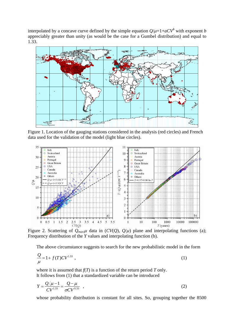
Figure 1. Location of the gauging stations considered in the analysis (red circles) and French data used for the validation of the model (light blue circles).

Figure 2. Scattering of Qmax/µ data in (CV(Q), Q/µ) plane and interpolating functions (a); Frequency distribution of the Y values and interpolating function (b).

The above circumstance suggests to search for the new probabilistic model in the form

33.1)(1 CVTfQ+=

µ , (1)

where it is assumed that f(T) is a function of the return period T only. It follows from (1) that a standardized variable can be introduced

33.033.1

1CVQ

CVQY

σµµ −

=−

= , (2)

whose probability distribution is constant for all sites. So, grouping together the 8500

maximum observed values of Y and estimating the empirical non exceedance frequency of each value, the result shown in Figure 2b is obtained. From the plot it turns out that the experimental data can be interpolated by a curve whose central part can be approximated by a linear function of ln T:

TY ln80.037.0 += , (3)

that in terms of the variable Q/µ becomes

33.1)ln80.037.0(1 CVTQ++=

µ. (4)

Equation (3) or, equivalently, Equation (4) yield the analytical expression of the MG model. Thanks to the great amount of data referring to different geographical areas of the Earth, the model can be considered quite general and so it can be applied to large areas such as Europe, Canada, USA and Australia.

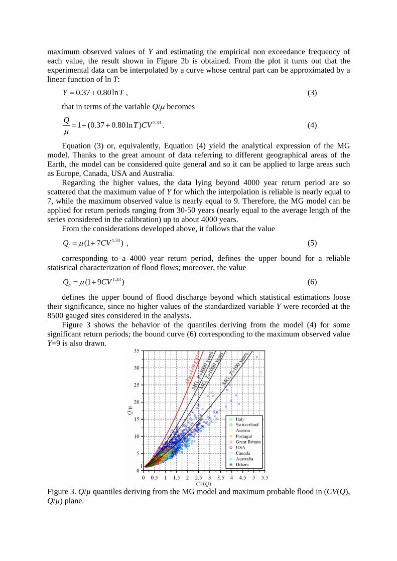
Regarding the higher values, the data lying beyond 4000 year return period are so scattered that the maximum value of Y for which the interpolation is reliable is nearly equal to 7, while the maximum observed value is nearly equal to 9. Therefore, the MG model can be applied for return periods ranging from 30-50 years (nearly equal to the average length of the series considered in the calibration) up to about 4000 years.

From the considerations developed above, it follows that the value

)71( 33.1CVQl += µ , (5)

corresponding to a 4000 year return period, defines the upper bound for a reliable statistical characterization of flood flows; moreover, the value

)91( 33.1CVQb += µ (6)

defines the upper bound of flood discharge beyond which statistical estimations loose their significance, since no higher values of the standardized variable Y were recorded at the 8500 gauged sites considered in the analysis.

Figure 3 shows the behavior of the quantiles deriving from the model (4) for some significant return periods; the bound curve (6) corresponding to the maximum observed value Y=9 is also drawn.

Figure 3. Q/µ quantiles deriving from the MG model and maximum probable flood in (CV(Q), Q/µ) plane.

In Table I the geographical areas considered in the analysis are indicated together with

minimum, average and maximum values of CV of the historical series (CVmin, CVavr, CVmax), the maximum and minimum values of catchment areas (Amin, Amax) and the maximum observed values (Ymax) of the standardized variable Y defined by Equation (2).

State Continent Number of stations

Average size of

the seriesCVmin CVavr CVmax

Amin (km2)

Amax (km2) Ymax

Italy Europe 249 36 0.23 0.62 1.81 6.1 70091 8.26 Switzerland Europe 143 45 0.11 0.36 0.79 39 34550 7.10 Austria Europe 83 34 0.19 0.79 1.91 10 1982 6.35 Portugal Europe 63 35 0.25 0.77 1.53 5.75 68429 6.34 Great Britain Europe 605 30 0.08 0.40 1.25 0.9 9948 7.81 Others Europe 101 56 0.14 0.49 1.49 23 51900 8.83 USA North America 6326 40 0.12 0.78 5.14 0.0259 831031 9.15 Canada North America 674 29 0.11 0.44 1.67 0.93 1270000 7.14 Australia Oceania 227 28 0.22 1.08 5.33 0.07 120000 5.16 Others South America 14 30 0.17 0.33 0.55 684 4640300 5.17 Others Asia 42 36 0.16 0.64 1.55 126 1000000 6.31 Others Africa 24 46 0.19 1.12 1.61 573 22500 5.19 ALL Varies 8551 38 0.08 0.71 5.33 0.0259 4640300 9.15

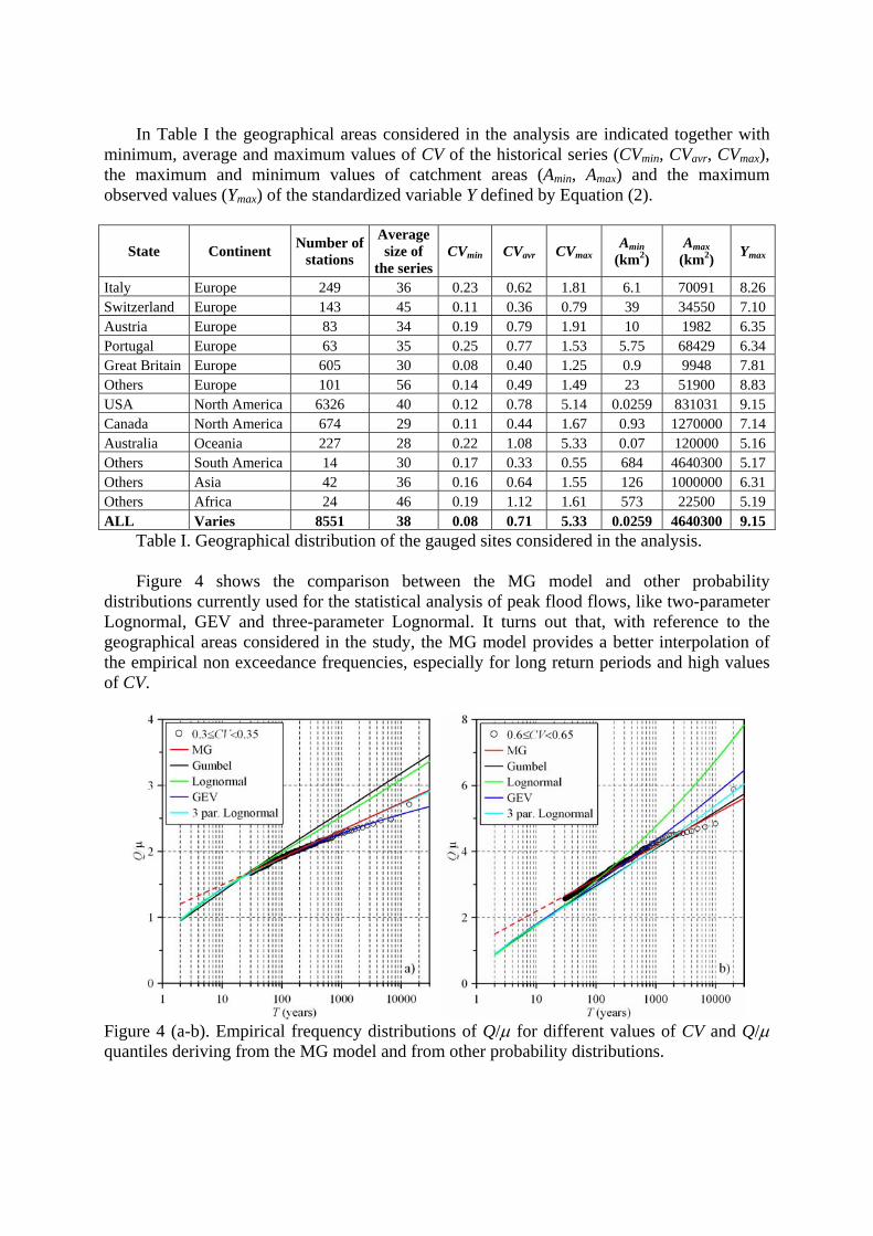
Table I. Geographical distribution of the gauged sites considered in the analysis. Figure 4 shows the comparison between the MG model and other probability

distributions currently used for the statistical analysis of peak flood flows, like two-parameter Lognormal, GEV and three-parameter Lognormal. It turns out that, with reference to the geographical areas considered in the study, the MG model provides a better interpolation of the empirical non exceedance frequencies, especially for long return periods and high values of CV.

Figure 4 (a-b). Empirical frequency distributions of Q/µ for different values of CV and Q/µ quantiles deriving from the MG model and from other probability distributions.

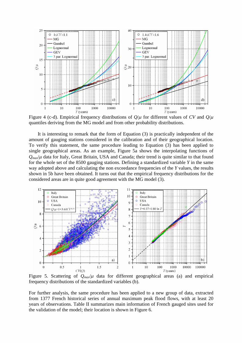
Figure 4 (c-d). Empirical frequency distributions of Q/µ for different values of CV and Q/µ quantiles deriving from the MG model and from other probability distributions.

It is interesting to remark that the form of Equation (3) is practically independent of the

amount of gauging stations considered in the calibration and of their geographical location. To verify this statement, the same procedure leading to Equation (3) has been applied to single geographical areas. As an example, Figure 5a shows the interpolating functions of Qmax/µ data for Italy, Great Britain, USA and Canada; their trend is quite similar to that found for the whole set of the 8500 gauging stations. Defining a standardized variable Y in the same way adopted above and calculating the non exceedance frequencies of the Y values, the results shown in 5b have been obtained. It turns out that the empirical frequency distributions for the considered areas are in quite good agreement with the MG model (3).

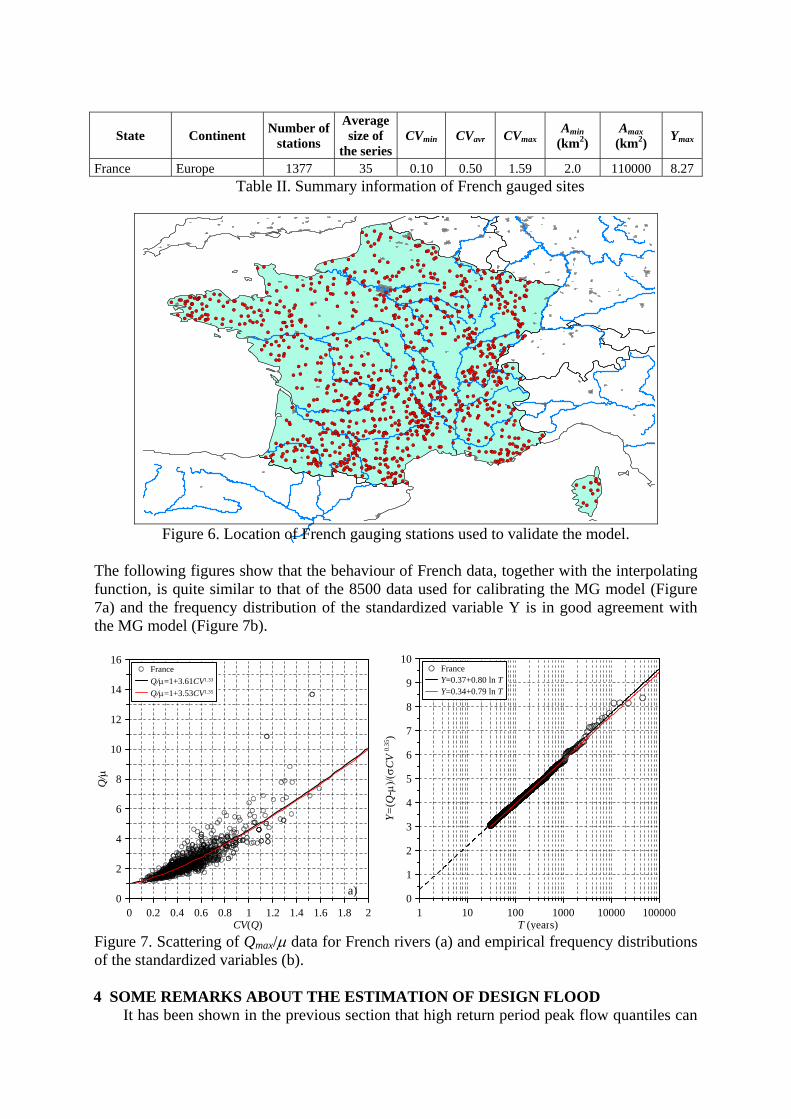
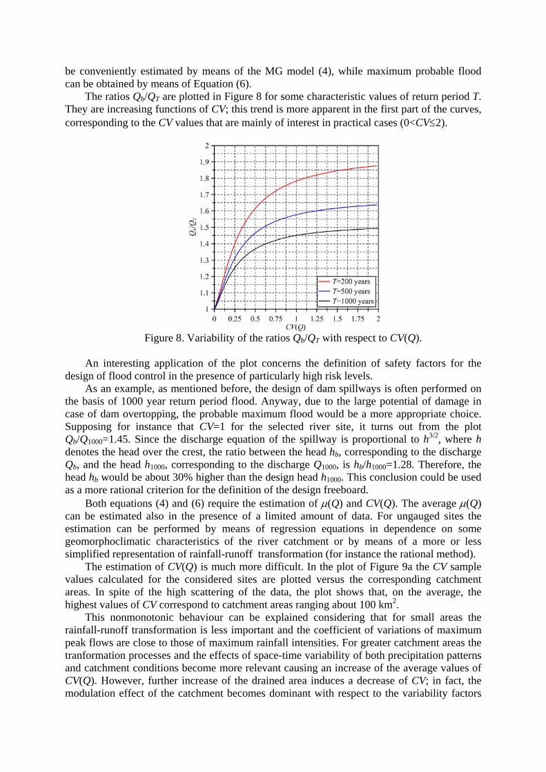
Figure 5. Scattering of Qmax/µ data for different geographical areas (a) and empirical frequency distributions of the standardized variables (b). For further analysis, the same procedure has been applied to a new group of data, extracted from 1377 French historical series of annual maximum peak flood flows, with at least 20 years of observations. Table II summarizes main information of French gauged sites used for the validation of the model; their location is shown in Figure 6.

State Continent Number of stations

Average size of

the seriesCVmin CVavr CVmax

Amin (km2)

Amax (km2) Ymax

France Europe 1377 35 0.10 0.50 1.59 2.0 110000 8.27 Table II. Summary information of French gauged sites

#S

#S

#S

#S

#S#S

#S

#S #S#S#S#S

#S

#S#S

#S#S #S

#S#S#S

#S

#S

#S

#S

#S

#S

#S

#S#S#S #S#S

#S#S#S#S#S#S#S

#S#S

#S#S#S#S

#S#S

#S

#S

#S

#S#S

#S#S

#S #S#S#S

#S#S

#S#S#S #S

#S#S

#S#S#S

#S#S#S#S

#S#S#S

#S#S#S

#S#S#S#S#S

#S

#S#S#S

#S#S#S#S#S#S#S

#S#S

#S#S#S #S

#S#S#S

#S#S

#S#S

#S

#S#S#S#S#S#S#S

#S

#S#S#S#S#S#S#S#S

#S

#S#S#S#S

#S#S#S#S

#S

#S

#S

#S

#S

#S

#S#S#S

#S#S#S#S

#S#S#S#S

#S #S#S

#S#S

#S #S#S#S

#S#S #S#S

#S#S#S

#S#S#S#S

#S#S

#S#S

#S#S

#S

#S

#S#S#S#S #S

#S

#S#S

#S#S#S#S#S#S#S#S

#S#S#S

#S

#S

#S#S

#S#S#S#S

#S

#S#S

#S #S#S#S#S#S

#S#S

#S

#S#S#S

#S#S#S

#S#S

#S#S#S#S

#S#S#S#S

#S

#S#S#S

#S#S

#S

#S#S#S#S#S

#S#S

#S

#S#S#S#S#S

#S#S#S

#S#S#S #S

#S#S#S#S#S#S

#S

#S#S#S

#S#S

#S#S#S

#S#S

#S#S

#S#S#S

#S

#S#S

#S#S#S#S

#S#S#S#S

#S

#S

#S#S#S#S

#S

#S#S#S

#S#S

#S#S#S

#S

#S

#S#S#S

#S#S

#S#S

#S

#S

#S#S#S#S#S#S#S#S#S #S#S

#S#S

#S#S#S

#S

#S

#S#S#S#S#S

#S#S

#S#S#S

#S#S

#S#S#S#S#S

#S#S#S#S#S

#S#S#S

#S#S

#S

#S#S#S

#S#S

#S

#S

#S

#S #S#S

#S

#S#S

#S #S#S#S

#S#S#S#S

#S

#S#S#S#S #S

#S#S#S

#S #S#S

#S#S#S

#S

#S#S

#S

#S#S#S#S#S #S

#S

#S#S #S#S

#S#S

#S

#S#S#S#S#S#S#S

#S

#S#S#S#S #S#S#S#S

#S#S#S

#S#S#S#S

#S#S#S#S#S

#S

#S #S#S#S#S

#S#S

#S

#S

#S#S#S#S

#S#S#S#S

#S#S#S#S

#S#S

#S

#S

#S#S

#S#S#S

#S

#S#S

#S#S#S

#S#S#S#S

#S#S#S

#S#S#S#S

#S #S#S#S#S#S

#S#S

#S#S#S

#S

#S#S#S

#S#S#S

#S

#S#S

#S#S#S

#S

#S#S

#S#S#S

#S#S

#S

#S#S

#S

#S

#S

#S

#S

#S

#S

#S

#S

#S

#S

#S

#S

#S#S#S

#S

#S

#S

#S#S

#S

#S

#S#S#S #S

#S#S

#S #S#S#S

#S#S

#S#S#S#S#S

#S#S

#S

#S

#S

#S#S#S#S#S #S#S#S

#S

#S#S

#S #S#S#S#S#S #S#S #S

#S#S

#S#S#S#S#S

#S

#S

#S

#S

#S

#S#S#S

#S#S#S

#S

#S

#S

#S

#S

#S#S

#S#S

#S

#S

#S#S

#S

#S

#S

#S

#S

#S

#S

#S

#S

#S

#S

#S

#S

#S

#S

#S

#S

#S

#S

#S

#S#S

#S

#S

#S#S

#S

#S

#S

#S

#S

#S

#S

#S

#S

#S#S#S

#S#S#S

#S#S#S#S

#S

#S#S#S#S

#S#S

#S

#S

#S#S#S

#S

#S#S

#S#S

#S

#S#S#S

#S

#S#S

#S#S#S

#S#S

#S

#S#S#S

#S#S#S#S

#S#S

#S

#S#S#S#S

#S

#S#S#S #S#S#S

#S#S#S#S

#S#S

#S#S

#S#S#S#S

#S #S

#S

#S

#S#S

#S#S#S#S

#S

#S

#S

#S#S #S#S

#S#S

#S#S

#S

#S#S#S#S

#S#S#S#S#S

#S

#S#S

#S

#S#S #S#S

#S#S

#S#S

#S #S#S

#S#S

#S#S#S

#S#S#S

#S#S

#S#S

#S#S

#S#S#S

#S#S#S

#S

#S#S

#S

#S

#S#S#S#S

#S#S#S

#S#S#S#S#S

#S#S #S #S

#S#S#S

#S#S

#S

#S#S#S

#S

#S

#S

#S#S#S#S#S#S#S#S

#S#S

#S

#S

#S

#S

#S#S

#S

#S#S

#S#S#S

#S#S#S

#S#S

#S#S#S #S #S#S#S#S#S#S

#S#S

#S#S#S#S#S

#S#S#S

#S

#S#S

#S#S

#S

#S

#S#S#S

#S#S

#S

#S#S

#S

#S #S#S#S#S

#S#S#S#S#S

#S#S

#S#S

#S#S#S#S

#S#S

#S#S

#S

#S

#S#S#S

#S#S#S#S

#S

#S

#S#S

#S

#S#S#S#S#S

#S#S#S#S#S#S#S

#S#S#S

#S

#S

#S

#S#S#S

#S

#S#S

#S#S

#S

#S

#S#S#S#S#S #S

#S#S#S

#S

#S

#S

#S #S#S

#S

#S#S#S

#S #S#S#S

#S#S#S

#S

#S

#S#S#S

#S#S#S

#S#S

#S#S#S#S#S#S#S

#S#S#S

#S#S#S

#S

#S#S

#S#S

#S#S

#S#S

#S

#S#S

#S#S#S#S#S

#S#S

#S

#S

#S#S#S#S#S

#S

#S#S#S

#S

#S#S#S

#S#S #S#S#S#S#S

#S

#S

#S#S#S#S#S#S

#S#S#S

#S#S#S#S

#S

#S

#S#S #S

#S#S#S#S#S

Figure 6. Location of French gauging stations used to validate the model.

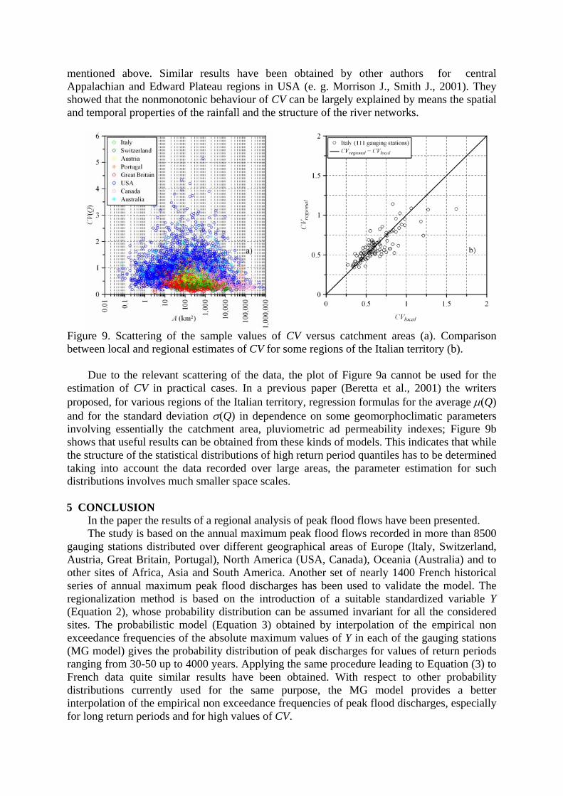
The following figures show that the behaviour of French data, together with the interpolating function, is quite similar to that of the 8500 data used for calibrating the MG model (Figure 7a) and the frequency distribution of the standardized variable Y is in good agreement with the MG model (Figure 7b).

0 0.2 0.4 0.6 0.8 1 1.2 1.4 1.6 1.8 2CV(Q)

0

2

4

6

8

10

12

14

16

Q/µ

FranceQ/µ=1+3.61CV1.33

Q/µ=1+3.53CV1.35

a)

1 10 100 1000 10000 100000T (years)

0

1

2

3

4

5

6

7

8

9

10

Y=(Q

-µ)/(σC

V 0.

35)

FranceY=0.37+0.80 ln TY=0.34+0.79 ln T

Figure 7. Scattering of Qmax/µ data for French rivers (a) and empirical frequency distributions of the standardized variables (b). 4 SOME REMARKS ABOUT THE ESTIMATION OF DESIGN FLOOD

It has been shown in the previous section that high return period peak flow quantiles can

be conveniently estimated by means of the MG model (4), while maximum probable flood can be obtained by means of Equation (6).

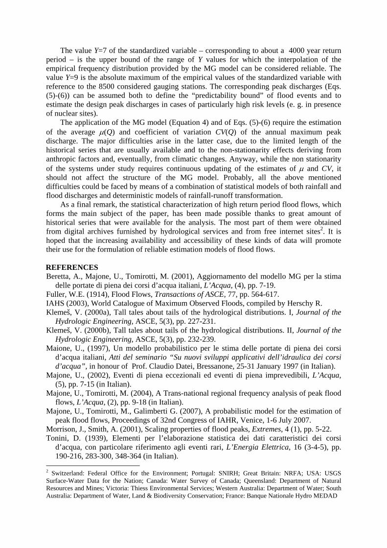
The ratios Qb/QT are plotted in Figure 8 for some characteristic values of return period T. They are increasing functions of CV; this trend is more apparent in the first part of the curves, corresponding to the CV values that are mainly of interest in practical cases (0<CV≤2).

Figure 8. Variability of the ratios Qb/QT with respect to CV(Q).

An interesting application of the plot concerns the definition of safety factors for the

design of flood control in the presence of particularly high risk levels. As an example, as mentioned before, the design of dam spillways is often performed on

the basis of 1000 year return period flood. Anyway, due to the large potential of damage in case of dam overtopping, the probable maximum flood would be a more appropriate choice. Supposing for instance that CV=1 for the selected river site, it turns out from the plot Qb/Q1000=1.45. Since the discharge equation of the spillway is proportional to h3/2, where h denotes the head over the crest, the ratio between the head hb, corresponding to the discharge Qb, and the head h1000, corresponding to the discharge Q1000, is hb/h1000=1.28. Therefore, the head hb would be about 30% higher than the design head h1000. This conclusion could be used as a more rational criterion for the definition of the design freeboard.

Both equations (4) and (6) require the estimation of µ(Q) and CV(Q). The average µ(Q) can be estimated also in the presence of a limited amount of data. For ungauged sites the estimation can be performed by means of regression equations in dependence on some geomorphoclimatic characteristics of the river catchment or by means of a more or less simplified representation of rainfall-runoff transformation (for instance the rational method).

The estimation of CV(Q) is much more difficult. In the plot of Figure 9a the CV sample values calculated for the considered sites are plotted versus the corresponding catchment areas. In spite of the high scattering of the data, the plot shows that, on the average, the highest values of CV correspond to catchment areas ranging about 100 km2.

This nonmonotonic behaviour can be explained considering that for small areas the rainfall-runoff transformation is less important and the coefficient of variations of maximum peak flows are close to those of maximum rainfall intensities. For greater catchment areas the tranformation processes and the effects of space-time variability of both precipitation patterns and catchment conditions become more relevant causing an increase of the average values of CV(Q). However, further increase of the drained area induces a decrease of CV; in fact, the modulation effect of the catchment becomes dominant with respect to the variability factors

mentioned above. Similar results have been obtained by other authors for central Appalachian and Edward Plateau regions in USA (e. g. Morrison J., Smith J., 2001). They showed that the nonmonotonic behaviour of CV can be largely explained by means the spatial and temporal properties of the rainfall and the structure of the river networks.

Figure 9. Scattering of the sample values of CV versus catchment areas (a). Comparison between local and regional estimates of CV for some regions of the Italian territory (b).

Due to the relevant scattering of the data, the plot of Figure 9a cannot be used for the estimation of CV in practical cases. In a previous paper (Beretta et al., 2001) the writers proposed, for various regions of the Italian territory, regression formulas for the average µ(Q) and for the standard deviation σ(Q) in dependence on some geomorphoclimatic parameters involving essentially the catchment area, pluviometric ad permeability indexes; Figure 9b shows that useful results can be obtained from these kinds of models. This indicates that while the structure of the statistical distributions of high return period quantiles has to be determined taking into account the data recorded over large areas, the parameter estimation for such distributions involves much smaller space scales.

5 CONCLUSION

In the paper the results of a regional analysis of peak flood flows have been presented. The study is based on the annual maximum peak flood flows recorded in more than 8500

gauging stations distributed over different geographical areas of Europe (Italy, Switzerland, Austria, Great Britain, Portugal), North America (USA, Canada), Oceania (Australia) and to other sites of Africa, Asia and South America. Another set of nearly 1400 French historical series of annual maximum peak flood discharges has been used to validate the model. The regionalization method is based on the introduction of a suitable standardized variable Y (Equation 2), whose probability distribution can be assumed invariant for all the considered sites. The probabilistic model (Equation 3) obtained by interpolation of the empirical non exceedance frequencies of the absolute maximum values of Y in each of the gauging stations (MG model) gives the probability distribution of peak discharges for values of return periods ranging from 30-50 up to 4000 years. Applying the same procedure leading to Equation (3) to French data quite similar results have been obtained. With respect to other probability distributions currently used for the same purpose, the MG model provides a better interpolation of the empirical non exceedance frequencies of peak flood discharges, especially for long return periods and for high values of CV.

The value Y=7 of the standardized variable – corresponding to about a 4000 year return period – is the upper bound of the range of Y values for which the interpolation of the empirical frequency distribution provided by the MG model can be considered reliable. The value Y=9 is the absolute maximum of the empirical values of the standardized variable with reference to the 8500 considered gauging stations. The corresponding peak discharges (Eqs. (5)-(6)) can be assumed both to define the “predictability bound” of flood events and to estimate the design peak discharges in cases of particularly high risk levels (e. g. in presence of nuclear sites).

The application of the MG model (Equation 4) and of Eqs. (5)-(6) require the estimation of the average µ(Q) and coefficient of variation CV(Q) of the annual maximum peak discharge. The major difficulties arise in the latter case, due to the limited length of the historical series that are usually available and to the non-stationarity effects deriving from anthropic factors and, eventually, from climatic changes. Anyway, while the non stationarity of the systems under study requires continuous updating of the estimates of µ and CV, it should not affect the structure of the MG model. Probably, all the above mentioned difficulties could be faced by means of a combination of statistical models of both rainfall and flood discharges and deterministic models of rainfall-runoff transformation.

As a final remark, the statistical characterization of high return period flood flows, which forms the main subject of the paper, has been made possible thanks to great amount of historical series that were available for the analysis. The most part of them were obtained from digital archives furnished by hydrological services and from free internet sites2. It is hoped that the increasing availability and accessibility of these kinds of data will promote their use for the formulation of reliable estimation models of flood flows. REFERENCES Beretta, A., Majone, U., Tomirotti, M. (2001), Aggiornamento del modello MG per la stima

delle portate di piena dei corsi d’acqua italiani, L’Acqua, (4), pp. 7-19. Fuller, W.E. (1914), Flood Flows, Transactions of ASCE, 77, pp. 564-617. IAHS (2003), World Catalogue of Maximum Observed Floods, compiled by Herschy R. Klemeš, V. (2000a), Tall tales about tails of the hydrological distributions. I, Journal of the

Hydrologic Engineering, ASCE, 5(3), pp. 227-231. Klemeš, V. (2000b), Tall tales about tails of the hydrological distributions. II, Journal of the

Hydrologic Engineering, ASCE, 5(3), pp. 232-239. Maione, U., (1997), Un modello probabilistico per le stima delle portate di piena dei corsi

d’acqua italiani, Atti del seminario “Su nuovi sviluppi applicativi dell’idraulica dei corsi d’acqua”, in honour of Prof. Claudio Datei, Bressanone, 25-31 January 1997 (in Italian).

Majone, U., (2002), Eventi di piena eccezionali ed eventi di piena imprevedibili, L’Acqua, (5), pp. 7-15 (in Italian).

Majone, U., Tomirotti, M. (2004), A Trans-national regional frequency analysis of peak flood flows, L’Acqua, (2), pp. 9-18 (in Italian).

Majone, U., Tomirotti, M., Galimberti G. (2007), A probabilistic model for the estimation of peak flood flows, Proceedings of 32nd Congress of IAHR, Venice, 1-6 July 2007.

Morrison, J., Smith, A. (2001), Scaling properties of flood peaks, Extremes, 4 (1), pp. 5-22. Tonini, D. (1939), Elementi per l’elaborazione statistica dei dati caratteristici dei corsi

d’acqua, con particolare riferimento agli eventi rari, L’Energia Elettrica, 16 (3-4-5), pp. 190-216, 283-300, 348-364 (in Italian).

2 Switzerland: Federal Office for the Environment; Portugal: SNIRH; Great Britain: NRFA; USA: USGS Surface-Water Data for the Nation; Canada: Water Survey of Canada; Queensland: Department of Natural Resources and Mines; Victoria: Thiess Environmental Services; Western Australia: Department of Water; South Australia: Department of Water, Land & Biodiversity Conservation; France: Banque Nationale Hydro MEDAD

Documents

THE MG MODEL FOR THE ESTIMATION OF PEAK FLOOD FLOWS, application to French rivers