Embed Size (px)
Citation preview

The Microstructure of Spoken Word Recognition
by
James Stephen Magnuson
Submitted in Partial Fulfillment
of the
Requirements for the Degree
Doctor of Philosophy
Supervised by
Professor Michael K. Tanenhaus
and
Professor Richard N. Aslin
Department of Brain and Cognitive Sciences
The College
Arts and Sciences
University of Rochester
Rochester, New York
2001

ii
Dedication
To Inge-Marie Eigsti, for your love and support, advice on research and
everything else, picking me up when I’m down, and making grad school a whole lot
of fun.
iii
Curriculum Vitae
The author was born December 19th, 1968, in St. Paul, Minnesota, and grew
up on a farm 50 miles north of the Twin Cities. He received the A.B. degree in
linguistics with honors from the University of Chicago in 1993. After two years as an
intern researcher at Advanced Telecommunications Research Human Information
Processing Laboratories in Kyoto, Japan, he began the doctoral program in Brain and
Cognitive Sciences at the University of Rochester.
The author worked in the labs of Professor Michael Tanenhaus and Professor
Mary Hayhoe in his first three years at Rochester. In both labs, he used eye tracking
as an incidental measure of processing (language processing in the former, visuo-
spatial working memory in the latter). As his dissertation work focused on spoken
word recognition, Michael Tanenhaus continued as his primary advisor, and Professor
Richard Aslin became his co-advisor.
The author was supported by a National Science Foundation Graduate
Research Fellowship (1995-1998), a University of Rochester Sproull Fellowship
(1998-2000), and a Grant-in-Aid-of-Research from the National Academy of
Sciences through Sigma Xi. He received the M.A. degree in Brain and Cognitive
Sciences in 2000.
iv
Acknowledgements
My parents, through life-long example, have taught me the importance of
family and hard work. I am grateful for the sacrifices they made, and the love and
support they gave me, which made it possible for me to be writing this today.
Several middle- and high-school teachers encouraged and inspired me in an
environment where intellectual pursuits were not always valued: Mary Ruprecht,
David Jaeger, Tim Johnson, Kay Pekel, and Howard Lewis. Terry and Susan
Wolkerstorfer played instrumental roles in my skin-of-the-teeth acceptance to the
University of Chicago, and have been great friends since. During a year off, I had
some adventures and seriously considered not returning to college. I thank Henry
Bromelkamp for ‘firing’ me and encouraging me to finish.
At Chicago, Nancy Stein’s introductory lecture for “Cognition and Learning”
first got me hooked on cognitive science. My interest grew into passion under
Howard Nusbaum’s tutelage. His enthusiasm and curiosity inspired my own, and I
will always look up to Howard’s example. I learned working for Gerd Gigerenzer that
science ought to be a lot of fun. At ATR in Japan, Reiko Akahane-Yamada was my
teacher and role model; her example confirmed my decision to pursue a Ph.D. I also
learned a lot from Yoh’ichi Tohkura, Hideki Kawahara, Eric Vatikiosis-Bateson,
Kevin Munhall, Winifred Strange, and John Pruitt.
I am extremely fortunate to have been able to pursue my Ph.D. at Rochester.
Mike Tanenhaus always provided just the right mixture of guidance, support and
freedom. Throughout the challenges of graduate school, Mike’s constant
encouragement, wit, and the occasional gourmet Asian feast helped keep me going.
Mary Hayhoe taught me a lot about how to tackle very difficult aspects of perception
and cognition experimentally. Her approach to perception and action in natural
contexts has had a huge impact on my interests and thinking. Dick Aslin is always
ready with sage advice on any topic. His Socratic knack for asking the question that
cuts to the essence of a problem has led me out of many intellectual and experimental

v
jams. I thank Joyce McDonnough for being part of my proposal committee, and
James Allen for being a member of my dissertation committee.
An especially important part of my experience at Rochester was collaborating
with post-docs and other students. Paul Allopenna taught me a lot about speech,
neural networks, risotto, and the guitar, and helped me through some difficult periods.
Delphine Dahan let me join her on three elegant projects. Paul and Delphine were
wonderful mentors, and the projects I did with them led to the work reported here.
Dave Bensinger showed me how to keep things in perspective. I’m still learning from
my current collaborators, Craig Chambers, Jozsef Fiser, and Bob McMurray.
My graduate school experience was shaped largely by a number of fellow
students, post-docs and friends, but in particular, Craig Chambers, Marie Coppola,
Jozsef Fiser, Josh Fitzgerald, Carla Hudson, Ruskin Hunt, Cornell Juliano, Sheryl
Knowlton, Toby Mintz, Seth Pollak, Jenny Saffran, Annie Senghas, Steve Shimozaki,
Michael Spivey, Julie Sedivy, and Whitney Tabor.
I was completely dependent on the expertise, encouragement and friendly
faces) of administrators and technical staff in BCS and the Center for Visual
Sciences, especially Bette McCormick, Kathy Corser, Jennifer Gillis, Teresa
Williams, Barb Arnold, Judy Olevnik, and Bill Vaughn. Several research assistants in
the Tanenhaus lab provided invaluable help running subjects and coding data. Dana
Subik was especially helpful and fun to work with, and provided the organization,
good humor, and patience that allowed me to finish on time.
It’s only a slight exaggeration to say that I owe my sanity and new job to
hockey. I thank Greg Carlson, George Ferguson, and the Rochester Rockets for
getting me back into hockey. Moshi-Moshi Neko and Henri Matisse were soothing
influences, and made sure I exercised everyday.
I’m grateful for support from a National Science Foundation Graduate
Research Fellowship, a University of Rochester Sproull Fellowship, a Grant-in-Aid-
of-Research from the National Academy of Sciences through Sigma Xi, and from
grants awarded to my advisors, M. Tanenhaus, M. Hayhoe, and R. Aslin.
vi
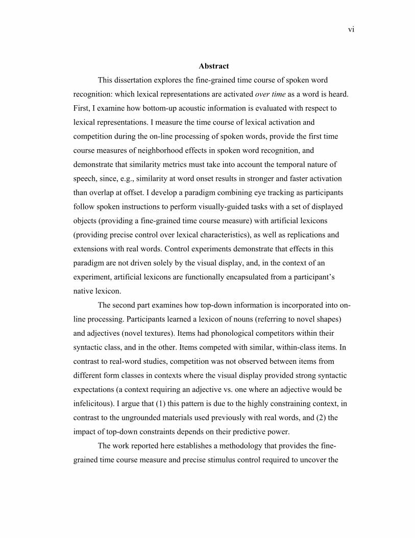
Abstract
This dissertation explores the fine-grained time course of spoken word
recognition: which lexical representations are activated over time as a word is heard.
First, I examine how bottom-up acoustic information is evaluated with respect to
lexical representations. I measure the time course of lexical activation and
competition during the on-line processing of spoken words, provide the first time
course measures of neighborhood effects in spoken word recognition, and
demonstrate that similarity metrics must take into account the temporal nature of
speech, since, e.g., similarity at word onset results in stronger and faster activation
than overlap at offset. I develop a paradigm combining eye tracking as participants
follow spoken instructions to perform visually-guided tasks with a set of displayed
objects (providing a fine-grained time course measure) with artificial lexicons
(providing precise control over lexical characteristics), as well as replications and
extensions with real words. Control experiments demonstrate that effects in this
paradigm are not driven solely by the visual display, and, in the context of an
experiment, artificial lexicons are functionally encapsulated from a participant’s
native lexicon.
The second part examines how top-down information is incorporated into on-
line processing. Participants learned a lexicon of nouns (referring to novel shapes)
and adjectives (novel textures). Items had phonological competitors within their
syntactic class, and in the other. Items competed with similar, within-class items. In
contrast to real-word studies, competition was not observed between items from
different form classes in contexts where the visual display provided strong syntactic
expectations (a context requiring an adjective vs. one where an adjective would be
infelicitous). I argue that (1) this pattern is due to the highly constraining context, in
contrast to the ungrounded materials used previously with real words, and (2) the
impact of top-down constraints depends on their predictive power.
The work reported here establishes a methodology that provides the fine-
grained time course measure and precise stimulus control required to uncover the
vii
microstructure of spoken word recognition. The results provide constraints on
theories of word recognition, as well as language processing more generally, since
lexical representations are implicated in aspects of syntactic, semantic and discourse
processing.
viii
Table of Contents
Dedication ..................................................................................................................... ii
Curriculum Vitae ......................................................................................................... iii
Acknowledgements...................................................................................................... iv
List of Tables ................................................................................................................ x
List of Figures .............................................................................................................. xi
Foreword ..................................................................................................................... xii
Chapter 1: Introduction and overview ................................................................ 1 The macrostructure of spoken word recognition .......................................................... 3
The microstructure of spoken word recognition........................................................... 6
Chapter 2: The “visual world” paradigm ......................................................... 10 The apparatus and rationale ........................................................................................ 10
Vision and eye movements in natural, ongoing tasks................................................. 13
Language-as-product vs. language-as-action.............................................................. 17
The microstructure of lexical access: Cohorts and rhymes ........................................ 18
Chapter 3: Studying time course with an artificial lexicon ......................... 26 Experiment 1............................................................................................................... 29
Method ................................................................................................................ 29 Results................................................................................................................. 34 Discussion........................................................................................................... 39
Experiment 2............................................................................................................... 39
Method ................................................................................................................ 40 Results................................................................................................................. 40 Discussion........................................................................................................... 43
Discussion of Experiments 1 and 2............................................................................. 43
Chapter 4: Replication with English stimuli ................................................... 46 Experiment 3............................................................................................................... 47
Methods............................................................................................................... 47 Predictions........................................................................................................... 49 Results................................................................................................................. 49 Discussion........................................................................................................... 55
Chapter 5: Do newly learned and native lexicons interact? ........................ 57 Experiment 4............................................................................................................... 58
Methods............................................................................................................... 58
ix
Predictions........................................................................................................... 62 First block ................................................................................................................... 62
Last block.................................................................................................................... 62
Results................................................................................................................. 62 Discussion........................................................................................................... 66 Conclusion .......................................................................................................... 69
Chapter 6: Top-down constraints on word recognition................................ 70 Experiment 5............................................................................................................... 73
Methods............................................................................................................... 73 Predictions........................................................................................................... 78 Results................................................................................................................. 79 Discussion........................................................................................................... 82
Chapter 7: Summary and Conclusions ............................................................. 84 References................................................................................................................... 86
Appendix: Materials used in Experiment 3 ................................................................ 95

x
List of Tables
Table 3.1: Accuracy in training and testing in Experiment 1. .................................... 36
Table 3.2: Accuracy in training and testing in Experiment 2. .................................... 41
Table 4.1: Frequencies and neighborhood and cohort densities in Experiment 3. ..... 48
Table 5.1: Linguistic stimuli from Experiment 4........................................................ 59
Table 5.2: Progression of training and testing accuracy in Experiment 4. ................. 62
Table 6.1: Artificial lexicon used in Experiment 5..................................................... 74
Table 6.2: Progression of accuracy in Experiment 5. ................................................. 79

xi
List of Figures
Figure 1.1: A schematic of the language processing system. ....................................... 5
Figure 2.1: Eye tracking methodology........................................................................ 12
Figure 2.2: The block-copying task. ........................................................................... 13
Figure 2.3: Activations over time in TRACE. ............................................................ 20
Figure 2.4: Fixation proportions from Experiment 1 in Allopenna et al. (1998)........ 21
Figure 2.5: TRACE activations converted to response probabilities.......................... 24
Figure 3.1: Examples of 2AFC (top) and 4AFC displays from Experiments 1 and 2.31
Figure 3.2: Day 1 test (top) and Day 2 test (bottom) from Experiment 1................... 33
Figure 3.3: Cohort effects on Day 2 in Experiment 1................................................. 35
Figure 3.4: Rhyme effects on Day 2 in Experiment 1. ............................................... 37
Figure 3.5: Combined cohort and rhyme conditions in Experiment 2........................ 42
Figure 3.6: Effects of absent neighbors in Experiment 2............................................ 44
Figure 4.1: Main effects in Experiment 3. .................................................................. 51
Figure 4.2: Interactions of frequency with neighborhood and cohort density. ........... 52
Figure 4.3: Neighborhood density at levels of frequency and cohort density. ........... 53
Figure 4.4: Cohort density at levels of frequency and neighborhood density. ........... 54
Figure 5.1: Examples of visual stimuli from Experiment 4........................................ 60
Figure 5.2: Frequency effects on Day 1 (left) and Day 2 (right) of Experiment 4. .... 64
Figure 5.3: Density effects on Day 1 (left) and Day 2 (right) of Experiment 4.......... 65
Figure 6.1: The 9 shapes and 9 textures used in Experiment 5................................... 74
Figure 6.2: Critical noun conditions in Experiment 5................................................. 80
Figure 6.3: Critical adjective conditions in Experiment 5. ......................................... 81

xii
Foreword
All of the experiments reported here were carried out with Michael Tanenhaus
and Richard Aslin. Delphine Dahan collaborated on Experiments 1 and 2.
1
Chapter 1: Introduction and overview
Linguistic communication is perhaps the most astonishing aspect of human
cognition. In an instant, we transmit complex and abstract messages from one brain to
another. We convert a conceptual representation to a linguistic one, and concurrently
convert the linguistic representation to a series of motor commands that drive our
articulators. In the case of spoken language, the acoustic energy of these articulations
is transformed from mechanical responses of hair cells in our listener’s ears to a
cortical representation of acoustic events which in turn must be interpreted as
linguistic forms, which then are translated into conceptual information, which
(usually) is quite similar to the intended message.
Psycholinguistics is concerned largely with the mappings between conceptual
representations and linguistic forms, and between linguistic forms and acoustics.
Words provide the central interface in both of these mappings. Conceptual
information must be mapped onto series of word forms, and in the other direction,
words are where acoustics first map onto meaning. Some recent theories of sentence
processing suggest that word recognition is not merely an intermediary stage that
provides the input to syntactic and semantic processing. Instead, various results
suggest that much of syntactic and semantic knowledge is associated with the
representations of individual words in the mental lexicon (e.g., MacDonald,
Pearlmutter, and Seidenberg, 1994; Trueswell and Tanenhaus, 1994). In the domain
of spoken language, lexical knowledge is implicated in aspects of speech recognition
that were often previously viewed as pre-lexical (Andruski, Blumstein, and Burton,
1994; Marslen-Wilson and Warren, 1994). Thus, how lexical representations are
accessed during spoken word recognition has important implications for language
processing more generally.
However, a complicating factor in the study of spoken words is the temporal
nature of speech. Words are comprised of sequences of transient acoustic events.
Understanding how acoustics are mapped onto lexical representations requires that
2
we analyze the time course of lexical activation; knowing which words are activated
as a word is heard provides strong constraints on theories of word recognition.
The experiments we report here address two aspects of word recognition
where time course measures are crucial. The first set of experiments addresses how
the bottom-up acoustic signal is mapped onto linguistic representations. Spoken
words, unlike visual words, are not unitary objects that can persist in time. Spoken
words are comprised of series of overlapping, transient acoustic events. The input
must be processed in an incremental fashion. As a word unfolds in time, the set of
candidate representations potentially matching the bottom-up acoustic signal will
change (cf., e.g., Marslen-Wilson, 1987). Different theories of spoken word
recognition make different predictions about the nature of the activated competitor set
over time (e.g., Marslen-Wilson, 1987, vs. Luce and Pisoni, 1998); thus, we need to
be able to measure the activations of different sorts of competitors as words are
processed in order to distinguish between models.
In addition, top-down information sources are integrated with bottom-up
acoustic information during word recognition, as we will review shortly. Knowing
when and how top-down information sources are integrated will provide strong
constraints on the development of theories and models of language processing.
Specifically, we will examine whether a combination of highly predictive syntactic
and pragmatic information can constrain the lexical items considered as possible
matches to an input, or whether spoken word recognition initially operates primarily
on bottom-up information. While this question has been addressed before, the
pragmatic aspect – a visual display providing discourse constraints – is novel.
A further contribution of this dissertation is the development of a
methodology that addresses the psycholinguist’s perennial dilemma. Words in natural
languages do not fall, in sufficient numbers, into neat categories of combinations of
characteristics of interest, such as frequency and number of neighbors (similar
sounding words), making it difficult to conduct precisely controlled factorial
experiments. By creating artificial lexicons, we can instantiate just such categories. In

3
the rest of this chapter, we will set the stage for the experiments reported in this
dissertation by reviewing the macrostructure and microstructure of spoken word
recognition.
The macrostructure of spoken word recognition
A set of important empirical results must be accounted for by any theory of
spoken word recognition. These principles form what Marslen-Wilson (1993) referred
to as the macrostructure of spoken word recognition: the general constraints on
possible architectures of the language processing system from the perspective of
spoken word recognition. At the most general level, current models employ an
activation metaphor, in which a spoken input activates items in the lexicon as a
function of their similarity to the input and item-specific information (such as the
frequency of occurrence). Activated items compete for recognition, also as a function
of similarity and item-specific characteristics.
We will not extensively review the results supporting each of these
constraints. Instead, consider results from Luce and Pisoni (1998), which illustrate all
of the constraints. According to their Neighborhood Activation Model (NAM), lexical
items are predicted to be activated by a given input according to an explicit similarity
metric.1 The probability of identifying each item is given by its similarity to the input
multiplied by its log frequency of occurrence divided by the sum of all items’
frequency-weighted similarities. Similar items are called neighbors, and a word’s
neighborhood is defined as the sum of the log-frequency weighted similarities of all
words (the similarities between most words will effectively be zero). The rule that
generates single-point predictions of the difficulty of identifying words is called the
“frequency-weighted neighborhood probability rule”.
1 Typically, the metric is similar to that proposed by Coltheart, Davelaar, Jonasson and Besner (1977)
for visual word recognition (items are predicted to be activated by an input if they differ by no more
than one phoneme substitution, addition or deletion), or is based on confusion matrices collected for
diphones presented in noise.

4
Luce and Pisoni report that item frequency alone accounts for about 5% of the
variance in a variety of measures, including lexical decision response times, and
frequency-weighted neighborhood accounts for significantly more (16-21%). So first
we see that item characteristics (e.g., frequency) largely determine how quickly words
can be recognized. Second, the fact that neighborhood is a good predictor of
recognition time shows that (a) multiple items are being activated, (b) those items
compete for recognition (since recognition time is inversely proportional to the
number of competitors, weighted by frequency, suggesting that as an input is
processed, all words in the neighborhood are activated and competing), and (c) items
compete both as a function of similarity and frequency (frequency weighted
neighborhood accounts for 10 to 15% more variance than simple neighborhood).
At the macro level, there are four more central phenomena that models of
spoken word recognition should account for. First, there is form priming. Goldinger,
Luce and Pisoni (1989) reported that phonetically related words should cause
inhibitory priming. Given first one stimulus (e.g., “veer”) and then a related one (e.g.,
“bull”, where each phoneme is highly confusable with its counterpart in the first
stimulus), recognition should be slowed compared to a baseline condition where the
second stimulus follows an unrelated item. The reason inhibition is predicted is that
the first stimulus is predicted to activate both stimuli initially, but the second stimulus
will be inhibited by the first (assuming an architecture such as TRACE’s, or Luce,
Goldinger, Auer and Vitevitch’s [2000] implementation of the NAM, dubbed
“PARSYN”). If the second stimulus is presented before its corresponding word form
unit returns to its resting level of activation, its recognition will be slowed. These
effects have generated considerable controversy (see Monsell and Hirsh, 1998, for a
critical review). However, Luce et al. (2000) review a series of past studies and
present some new ones that provide compelling evidence for inhibitory form (or
“phonetic”) priming.
Second, there is associative or semantic priming, by which a word like “chair”
can prime a phonetically unrelated word like “table” due to their semantic

5
relatedness. Third, there is cross-modal priming (e.g., Tanenhaus, Leiman and
Seidenberg, 1979; Zwitserlood, 1989), in which words presented auditorily affect the
perception of phonologically or semantically related words presented visually.
Finally, there are context effects. These include syntactic and semantic effects, where
a listener is biased towards one interpretation of an ambiguous sequence by its
sentence (or larger discourse) context (see Tanenhaus and Lucas, 1987, for a review).
Acoustic-phonetic features
Phonemes
Word formsVisual word recognition
Visual word recognition
Spoken wordrecognition
SemanticsSemantics
LexiconLexicon
Syntax/ParsingSyntax/Parsing
Auditory processing of acoustic
input
Auditory processing of acoustic
input
Discourse/PragmaticsDiscourse/Pragmatics
Figure 1.1: A schematic of the language processing system.
Figure 1.1 shows schematically the components of the language processing
system implicated in the spoken word recognition literature. Components represented
by ‘clouds’ are not implemented in any current model of spoken word recognition
(although models for these exist in other areas of language research). These are
6
depicted as separate components merely for descriptive purposes; we will not discuss
the degree to which any of them can be considered independent modules here.
The microstructure of spoken word recognition
Marslen-Wilson (1993) contrasted two levels at which one could formulate a
processing theory. First, there are questions about the global properties of the
processing system. A theory based on such a “macrostructural” perspective focuses
on fairly coarse (but nonetheless important) questions such as what constraints there
are on the general class of possible models. For spoken word recognition, these
include the factors we discussed in the previous section. Armed with knowledge
about the general properties required of a model, one can proceed to the more precise,
“microstructural” level, and address fine-grained issues such as interactions among
processing predictions for specific stimuli, modeling and measuring the time course
of processing, and questions of how representations are learned.
There is no black-and-white distinction between macro- and microstructural
“levels.” Rather, there is a continuum. For example, Luce’s NAM (Luce, 1986; Luce
and Pisoni, 1998) identifies some global, macrostructural constraints, but at the same
time, makes such fine-grained predictions as response times for individual items.
Why, then, have we taken, “the microstructure of spoken word recognition,” as our
title? Two reasons are especially important.
First, as Marslen-Wilson (1993) implied, the time has come for research on
spoken word recognition to address the microstructure end of the continuum. There is
consensus on the general properties of the system, but the field lacks a realistic theory
or model with sufficient depth to account for microstructure, while maintaining
sufficient breadth to obey the known macrostructural constraints (in other words,
there are microtheories or micromodels of specific phenomena, but no sufficiently
general theories or models; cf. Nusbaum and Henly, 1992). The best-known, best-
worked out, explicit, implemented model of spoken word recognition remains the
TRACE model (McClelland and Elman, 1986). While it suffers from various

7
computational problems (e.g., Elman, 1989; Norris, 1994), and cannot account for a
number of basic speech perception phenomena, such as rate or talker normalization
(e.g., Elman, 1989), it is the best game in town sixteen years later. One central factor
in the slow rate of progress in developing theories of spoken word recognition has to
do with a lag between the development of models of microstructure (such as TRACE
and Cohort [e.g., Marslen-Wilson, 1987]) and sufficiently sensitive, direct and
continuous measures to distinguish between them. As we will discuss in Chapter 2,
the head-mounted eye tracking technique applied to language processing by
Tanenhaus and colleagues (e.g., Tanenhaus et al., 1995) represents a large advance in
our ability to measure the microstructure of language processing.
The second reason to focus on microstructure has to do with what we argue to
be an essential component of the microstructure approach: the use of precise
mathematical models, or, in the case of simulating models (such as non-deterministic
or incompletely understood neural networks), implemented models. Without precise,
implemented models, there are limits to our ability to address even global properties
of processing systems. Consider an example from visual perception.
“Pop-out” phenomena in visual search are well known (see Wolfe, 1996, for a
recent comprehensive review). Early explanations (which are still largely accepted)
appealed to pre-attentive vs. attentive processes and resulting parallel or serial
processing (e.g., Treisman and Gelade, 1980). Such verbal models appeared to be
quite powerful. Many researchers replicated the diagnostic pattern. For searches
based on a single feature, response time does not increase as the number of distractors
does, suggesting a parallel process. More complex searches for combinations of
features (or absence of features) lead to a linear increase in response time as the
number of distractors is increased, suggesting a serial search. Some, however, began
to question the parallel/serial distinction, even as it began to take on the luster of a
perceptual law.
For example, studies by Duncan and Humphreys (1989) indicated that some
processes diagnosed as “early” or pre-attentive were actually carried out rather late in

8
the visual system. Without a worked-out theory of attention that could explain why a
late process should be pre-attentive, the pre-attentive/attentive distinction was brought
into question. Duncan and Humphreys (1989), among others, questioned the
parallel/serial processing distinction. When precise, signal-detection-based models
were combined with greater gradations of stimuli, the distinction was shown to be
false; there is a continuum of processing difficulty that varies as a function of target
and distractor discriminability.
This example illustrates the potential hazards of focusing even on global,
macrostructural issues without precise models. However, psycholinguists seem
determined to repeat history. Consider the current debate in sentence processing
between proponents of constraint-based, lexicalist models (which are analogous to the
signal detection approach to visual search in that they consider stimulus-specific
attributes) and structural models (e.g., the garden-path model [e.g., Frazier and
Clifton, 1996], which claims that processing depends on structures a level of
abstraction apart from specific stimuli).
Tanenhaus (1995) made the case for the microstructure end of the continuum
in studying sentence processing, and argued that even global questions could not be
adequately addressed without precise, parameterized models. Clifton (1995) argued
that the conventional approach of addressing global questions (such as whether
human sentence processing is parallel or serial) remained the best course for progress.
Clifton, Villalta, Mohamed and Frazier (1999) reiterated this argument, and claimed
to refute recent evidence for parallelism (Pearlmutter and Mendelsohn, 1998) with a
null result using different stimuli.
This is exactly the style of reasoning Tanenhaus (1995) argued against, and
which proved so misleading in the study of visual search. Without item-specific
predictions, one cannot refute lexically-based – that is, item-based – models. Some
might argue that this is a flaw, since the purpose of theory building ought to be to
make broad, general predictions that capture the essence of a problem.
9
Furthermore, lexicalist models provide a precise and robust account of much
of the phenomena of sentence processing (although there are not yet any implemented
models of sufficient breadth and depth). Constraint-based models predict, as did
signal-detection models for visual search, that a continuum of processing patterns can
be observed depending on interactions among the characteristics of the stimuli used.
Without measuring the relevant characteristics for Clifton el al.’s (1999) stimuli, one
cannot quantify constraint-based predictions for their experiment.
In summary, what we mean by microstructure goes beyond the dichotomy
suggested by Marslen-Wilson (1993), to a continuum between macro- and
microstructural questions. As microstructural questions are becoming more central in
spoken word recognition, we must develop methods that allow both fine-grained time
course measures and precise control of stimulus-specific characteristics. The next
chapter is devoted to a review of the recent development of a fine-grained time-
course measure. The succeeding chapters combine the eye tracking measure with an
artificial lexicon paradigm which allows precise control over lexical attributes.

10
Chapter 2: The “visual world” paradigm
In typical psychophysical experiments, the goal is to isolate a component of
behavior to the greatest possible extent. Almost always, this entails removing the task
from a naturalistic context. While a great deal has been learned about perception and
cognition with this classical approach, it leaves open the possibility that perception
and cognition in natural, ongoing tasks may operate under very different constraints.
Recently, a handful of researchers have begun examining visual and motor
performance in more natural tasks (e.g., Hayhoe, 2000; Land and Lee, 1994; Land,
Mennie and Rusted, 1998; Ballard et al., 1997). The key methodological advance that
has allowed this change in focus is the development of head-mounted eye trackers
that allow relatively unrestricted body movements, and thus can provide a continuous
measure of visual performance during natural tasks. In this chapter, we will describe
the eye tracker used in the experiments described in the following chapters. Then, we
will briefly review its use in the study of vision, and the adaptation of this technique
for studying language processing.
The apparatus and rationale
An Applied Science Laboratories (ASL) 5000 series head-mounted eye
tracker was used for the first two experiments reported here. An SMI EyeLink, which
operates on similar principles, was used for the last three experiments. The tracker
consists mainly of two cameras mounted on a headband. One provides a near-infrared
image of the eye sampled at 60 Hz. The pupil center and first Purkinje reflection are
tracked by a combination of hardware and software in order to provide a constant
measure of the position of the eye relative to the head. The second camera (the
“scene” camera) is aligned with the subject’s line of sight (see Figure 2.1). Because it
is mounted on the headband and moves when the subject’s head does, it remains
aligned with the subject’s line of sight. Therefore, the position of the eye relative to

11
the head can be mapped onto scene camera coordinates through a calibration
procedure. The ASL software/hardware package provides a cross hair indicating
point-of-gaze superimposed on a videotape record from the scene camera. Accuracy
of this record (sampled at video frame rates of 30 Hz) is approximately 1 degree over
a range of +/- 25 degrees. An audio channel is recorded to the same videotape. Using
a Panasonic HI-8 VCR with synchronized sound and video, data is coded frame-by-
frame, and eye position is recorded with relation to visual and auditory stimuli. Visual
stimuli are displayed on a computer screen, and fluent speech is either spoken (in the
case of the Allopenna, Magnuson and Tanenhaus, 1998, study we will review below)
or played to the subject over headphones using standard Macintosh PowerPC D-to-A
facilities.
The rationale for using eye movements to study cognition is that eye
movements are typically fairly automatic, and are under limited conscious control. On
average, we make 2-3 eye movements per second (although this can vary widely
depending on task constraints; Hayhoe, 2000), and we are unaware of most of them.
Furthermore, saccades are ballistic movements; once a saccade is launched, it cannot
be stopped. Given a properly constrained task, in which the subject must perform a
visually-guided action, eye movements can be given a functional interpretation. If
they follow a stimulus in a reliable, predictable fashion with minimal lag,2 they can be
interpreted as actions based on underlying decision mechanisms. Although there is
evidence that eye movements in unconstrained, free-viewing linguistics tasks are
highly correlated with linguistic stimuli (Cooper, 1974), all of the experiments in this
proposal will use visual-motor tasks in order to avoid the pitfalls of interpreting
unconstrained tasks (see Viviani, 1990).
2 We take 200 ms to be a reasonable estimate of the time required to plan and launch a saccade in this
task, given that the minimum latency is estimated to be between 150 and 180 ms in simple tasks
(e.g., Fischer, 1992; Saslow, 1967), whereas intersaccadic intervals in tasks like visual search fall in
the range of 200 to 300 ms (e.g., Viviani, 1990).

12
Subject's view(from scenecamera on
helmet)
Eyecamera
VCR
ASL/PC
Figure 2.1: Eye tracking methodology.

13
Vision and eye movements in natural, ongoing tasks
Models of visuo-spatial working memory have typically been concerned with
the limits of human working memory. Results from studies pushing working memory
to its limits have led to the proposal of modality-specific “slave” systems that provide
short-term stores. Usually, it is assumed that there are at least two such stores: the
articulatory loop, which supports verbal working memory, and the visuo-spatial
scratchpad (Baddeley and Hitch, 1974) or “inner scribe” (Logie, 1995), which
supports visual working memory. Recent research by Hayhoe and colleagues was
designed to complement such work with studies of how capacity limitations constrain
performance in natural, ongoing tasks carried out without added time or memory
pressures.
The prototypical task they use is block-copying (see Figure 2.2). Participants
are presented with a visual display (on a computer monitor or on a real board) that is
divided into three areas. The model area contains a pattern of blocks. The
participant’s task is to use blocks from the resource area to construct a copy of the
model pattern in the workspace. Eye and hand position are measured continuously as
the participant performs the task. The task is to use blocks displayed in the resource
(right monitor) to build a copy of the model (center) in the workspace (left). The
arrows and numbers indicate a typical fixation pattern during block copying. The
participant fixates the current block twice. At fixation 2, the participant picks up the
dark gray block. After fixation 4, the participant drops the block.
Workspace Model Resource
13 24
Figure 2.2: The block-copying task.
14
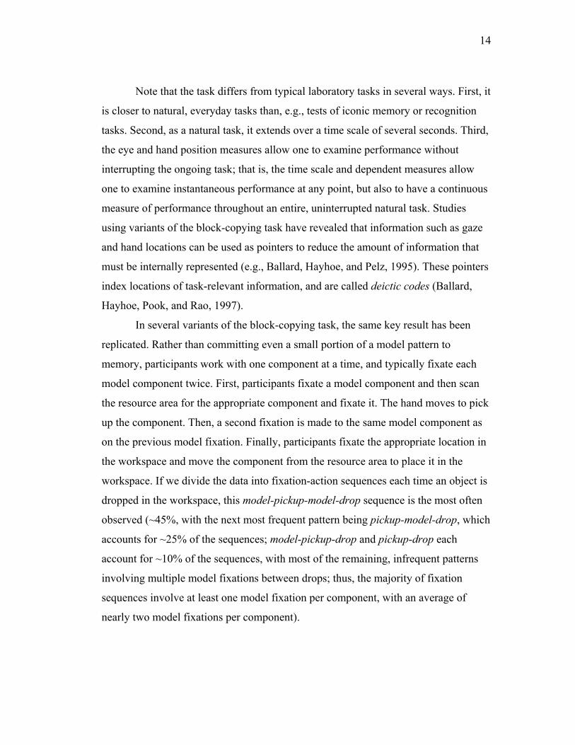
Note that the task differs from typical laboratory tasks in several ways. First, it
is closer to natural, everyday tasks than, e.g., tests of iconic memory or recognition
tasks. Second, as a natural task, it extends over a time scale of several seconds. Third,
the eye and hand position measures allow one to examine performance without
interrupting the ongoing task; that is, the time scale and dependent measures allow
one to examine instantaneous performance at any point, but also to have a continuous
measure of performance throughout an entire, uninterrupted natural task. Studies
using variants of the block-copying task have revealed that information such as gaze
and hand locations can be used as pointers to reduce the amount of information that
must be internally represented (e.g., Ballard, Hayhoe, and Pelz, 1995). These pointers
index locations of task-relevant information, and are called deictic codes (Ballard,
Hayhoe, Pook, and Rao, 1997).
In several variants of the block-copying task, the same key result has been
replicated. Rather than committing even a small portion of a model pattern to
memory, participants work with one component at a time, and typically fixate each
model component twice. First, participants fixate a model component and then scan
the resource area for the appropriate component and fixate it. The hand moves to pick
up the component. Then, a second fixation is made to the same model component as
on the previous model fixation. Finally, participants fixate the appropriate location in
the workspace and move the component from the resource area to place it in the
workspace. If we divide the data into fixation-action sequences each time an object is
dropped in the workspace, this model-pickup-model-drop sequence is the most often
observed (~45%, with the next most frequent pattern being pickup-model-drop, which
accounts for ~25% of the sequences; model-pickup-drop and pickup-drop each
account for ~10% of the sequences, with most of the remaining, infrequent patterns
involving multiple model fixations between drops; thus, the majority of fixation
sequences involve at least one model fixation per component, with an average of
nearly two model fixations per component).

15
Given such a simple task, why don’t participants encode and work on even
two or three components between model fixations, which would be well within the
range of short-term memory capacity? Ballard et al. (1997) have proposed that
memories for motor signals and eye or hand locations provide a more efficient
mechanism than could be afforded by a purely visual, unitary, imagistic
representation. In the block-copying paradigm, participants seem to encode simple
properties one at a time, rather than encoding complex representations of entire
components. For example, a fixation to a model component could be used to encode
the block’s color, and its location within the pattern. This might require encoding not
just the block’s color, but also the colors of its neighbors (which would indicate its
relative location). Alternatively, the block’s color and the signal indicating the
fixation coordinates could be encoded. With the color information, a fixation can be
made to the resource area to locate a block for the copy. The fixation coordinates
could serve as a pointer to the block’s location in the model (and all potential
information available at that location). Next, a saccade can be made back to the
fixation coordinates, and the information necessary for placing the picked-up block in
the workspace can be encoded.
Note that in the copying task, the second fixation is typically made back to
exactly the same place in the model. Why can’t the information that allows the
participant to fixate the same location be used to place the picked-up block in the
correct place in the workspace? Because that information is about an eye position –
the pointer – not about the relative location of the block in the pattern. The fixation
coordinates act as a pointer in the sense of the computer programming term: a small
information unit that represents a larger information unit simply by encoding its
location. Thus, very little information need be encoded internally at a given moment.
Perceptual pointers allow us to reference the external world and use it as memory, in
a just-in-time fashion. This hypothesis was inspired in part by an approach in
computer vision that greatly reduced the complexity of representations needed to
interact with the world. On the active or animate vision view (Bajcsy, 1985; Brooks,

16
1986; Ballard, 1991), much less complex representations of the world are needed
when sensors are deployed (e.g., camera saccades are made) in order to sample the
world frequently, in accord with task demands.
Hayhoe, Bensinger and Ballard (1998) reported compelling evidence for the
pointer hypothesis in human visuo-motor tasks. As participants performed the block-
copying task at a computer display, the color of an unworked model block was
sometimes changed during saccades to the model area (when the participant would be
functionally blind for the approximately 50 ms it takes to make a saccadic eye
movement). The color changes occurred either after a drop in the workspace (before
pickup), or after a pickup in the resource area (after pickup). Participants were
unaware of the majority of color changes, according to their verbal reports. However,
fixation durations revealed that performance was affected. Fixation durations were
slightly, but not reliably, longer (+43 ms) when a color change occurred before
pickup compared to a control when no color change occurred. When the color change
occurred after pickup, fixation durations were reliably longer (+103 ms) than when no
change occurred.
How do these results support the pointer hypothesis? Recall that the most
frequent fixation pattern was model-pickup-model-drop. When the change occurs
after pickup -- just after the participant has picked up a component from the resource
area and is about to fixate the corresponding model block again -- there is a relatively
large effect on performance. When the color change occurs before pickup -- just after
a participant has finished adding a component to the workspace -- there is a relatively
small effect. At this stage, according to the pointer hypothesis, color information is no
longer relevant; what had been encoded for the preceding pickup and drop can be
discarded, and this is reflected in the small increase in fixation duration.
Bensinger (1997) explored various alternatives to this explanation. He found
that the same basic results hold when: (a) participants can pick up as many
components as they like (in which case they still make two fixations per component,
but with sequences like model-pickup, model-pickup, model-drop, model-drop), (b)
17
images of complex natural objects are used rather than simple blocks, or (c) the
model area is only visible when the hand is in the resource area (in which case the
number of components being worked on drops when participants can pick up as many
components as they want, so as to minimize the number of workspace locations to be
recalled when the model is not visible).
Language-as-product vs. language-as-action
The studies we just reviewed reveal a completely different perspective of
visual behavior than classical methods for studying visuo-spatial working memory.
The discovery that multiple eye movements can substitute for complex memory
operations might not have emerged using conventional paradigms. Language research
also relies largely on classical, reductionist tasks, on the one hand, and, on the other,
on more natural tasks (such as cooperative dialogs) that do not lend themselves to
fine-grained analyses. Clark (1992) refers to this as the distinction between language-
as-product and language-as-action traditions.
In the language-as-product tradition, the emphasis is on using clever,
reductionist tasks to isolate components of hypothesized language processing
mechanisms. The benefit of this approach is the ability to make inferences about
mechanisms due to differences in measures such as response time or accuracy as a
function of minimal experimental manipulations. The cost is the potential loss of
ecological validity; as with vision, it is not certain that language-processing behavior
observed in artificial tasks will generalize to natural tasks. In the language-as-action
tradition, the emphasis is on language in natural contexts, with the obvious benefit of
studying behavior closer to that found “in the wild.” The cost is the difficulty of
making measurements at a fine enough scale to make inferences about anything but
the macrostructure of the underlying mechanisms.
The head-mounted eye-tracking paradigm provides the means of bringing the
two language research traditions closer together. As in the vision experiments,
subjects can be asked to perform relatively natural tasks. Eye movements provide a
18
continuous, fine-grained measure of performance, which allows (specially designed)
natural tasks to be analyzed at an even finer level than conventional measures from
the language-as-product tradition. To illustrate this, we will briefly review one study
of spoken word recognition using this technique (known as “the visual world
paradigm”).
The microstructure of lexical access: Cohorts and rhymes Allopenna, Magnuson and Tanenhaus (1998) extended some previous work
using this paradigm (Tanenhaus et al., 1995) to resolve a long-standing difference in
the predictions of two classes of models of spoken word recognition. “Alignment”
models (e.g., Marslen-Wilson’s Cohort model [1987] or Norris’ Shortlist model
[1994]) place a special emphasis on word onsets to solve the segmentation problem –
that is, finding word boundaries. Marslen-Wilson and Welsh (1978) proposed that an
optimal solution would be, starting from the onset of an utterance, to consider only
those word forms consistent with the utterance so far at any point. Given the stimulus
beaker, at the initial /b/, all /b/-initial word forms would form the cohort of words
accessed as possible matches to the input. As more of the stimulus is heard, the cohort
is whittled down (from /b/-initial to /bi/-initial to /bik/-initial, etc.) until a single
candidate remains. At that point, the word is recognized, and the process begins again
for the next word.3 In its revised form, as with the Shortlist model, Cohort maintains
its priority on word onsets (and thus constrains the size of the cohort) in an activation
framework by employing bottom-up inhibition. Lower-level units have bottom-up
inhibitory connections to words that do not contain them (tripling, on average, the
number of connections to each word in an architecture where phonemes connect to
words, compared to an architecture like TRACE’s, where there are only excitatory
bottom-up connections).
In contrast to alignment models’ emphasis on word onsets, continuous
activation models like TRACE (McClelland and Elman, 1986) and NAM/PARSYN
3 In cases where there ambiguity remains, the Cohort model’s selection and integration mechanisms
complete the segmentation decision.

19
(Luce and Pisoni, 1998; Luce et al., in press) are not designed to give priority to word
onsets. Words can become active at any point due to similarity to the input. The
advantage for items that share onsets with the input (which we will refer to as cohort
items, or cohorts) is still predicted, because active word units inhibit all other word
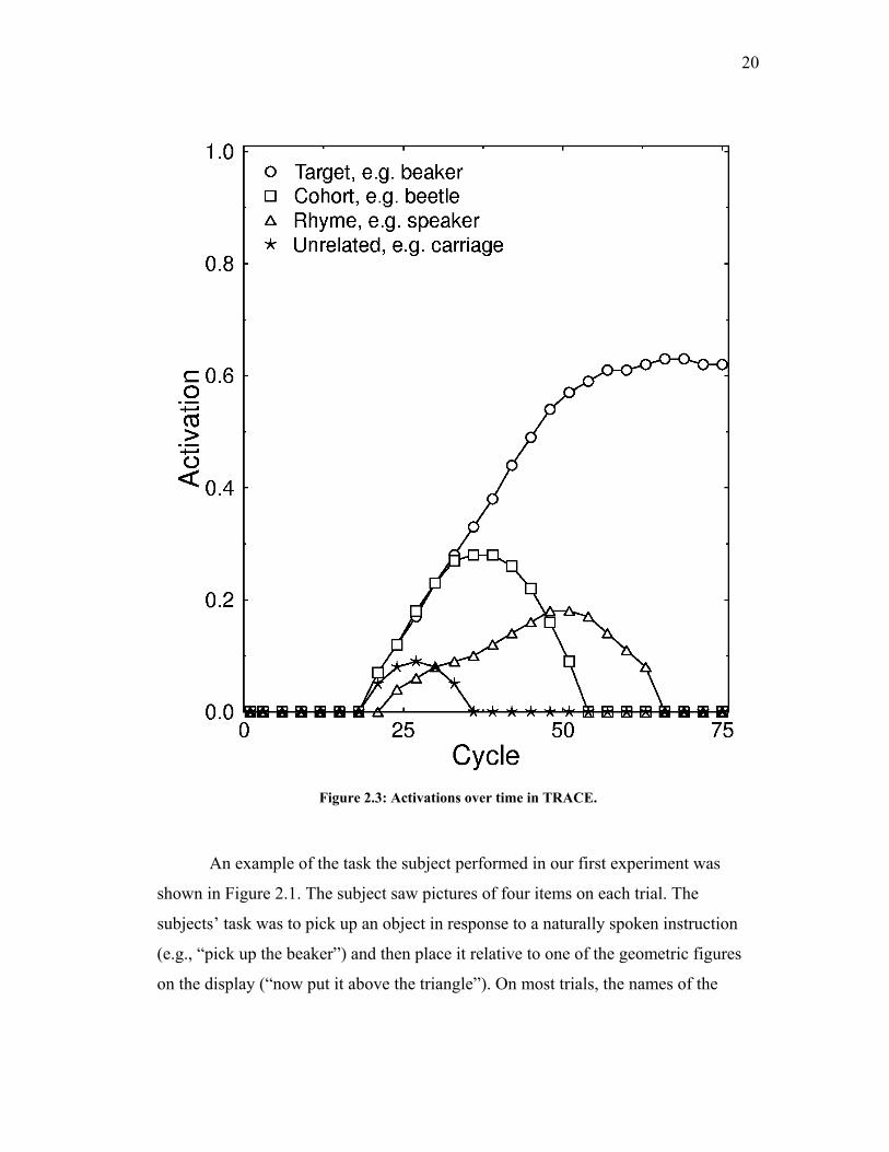
nodes. As shown in Figure 2.3, cohort items become activated sooner than, e.g.,
rhymes. Thus, cohort items (as well as the correct referent) inhibit rhymes and
prevent them from becoming as active as cohorts, despite their greater overall
similarity. Still, substantial rhyme activation is predicted by continuous activation
models, whereas in alignment models, an item like ‘speaker’ would not be predicted
to be activated by an input of ‘beaker.’
Until recently, there was ample evidence for cohort activation (e.g., Marslen-
Wilson and Zwitserlood, 1989), but there was no clear evidence for rhyme activation.
For example, weak rhyme effects had been reported in cross-modal and auditory-
auditory priming (Connine, Blasko and Titone, 1993; Andruski et al., 1994) when the
rhymes differed by only one or two phonetic features. The hints of rhyme effects left
open the possibility that conventional measures were simply not sensitive enough to
detect the robust, if relatively weak, rhyme activation predicted by models like
TRACE.4 Encouraged by the ability of the visual world paradigm to measure the time
course of activation among cohort items (Tanenhaus et al., 1995), Allopenna et al.
(1998) designed an experiment to take another look at rhyme effects.
4 This is especially true when null or weak results come from mediated tasks like cross-modal
priming, where the amount of priming one would expect was not specified by any explicit model.
Presumably, weak activation in one modality would result in even weaker activation spreading to the
other.
20
Figure 2.3: Activations over time in TRACE.
An example of the task the subject performed in our first experiment was
shown in Figure 2.1. The subject saw pictures of four items on each trial. The
subjects’ task was to pick up an object in response to a naturally spoken instruction
(e.g., “pick up the beaker”) and then place it relative to one of the geometric figures
on the display (“now put it above the triangle”). On most trials, the names of the
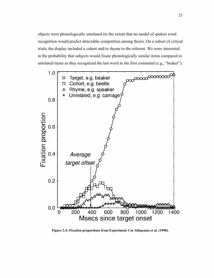
21
objects were phonologically unrelated (to the extent that no model of spoken word
recognition would predict detectable competition among them). On a subset of critical
trials, the display included a cohort and/or rhyme to the referent. We were interested
in the probability that subjects would fixate phonologically similar items compared to
unrelated items as they recognized the last word in the first command (e.g., “beaker”).
Figure 2.4: Fixation proportions from Experiment 1 in Allopenna et al. (1998).

22
Fixation probabilities averaged over 12 subjects and several sets of items are
shown in Figure 2.4. The data bear a remarkable resemblance to the TRACE
activations shown in Figure 2.3. However, those activations are from an open-ended
recognition process, and cannot be compared directly to fixation probabilities for two
reasons. First, probabilities sum to one, which is not a constraint on TRACE
activations. (Note that the fixation proportions in Figure 2.4 do not sum to one
because subjects begin each trial fixating a central cross; the probability of fixating
this cross is not shown.) Second, subjects could fixate only the items displayed during
each trial. We needed a linking hypothesis to relate TRACE activations to behavioral
data.
We addressed these two problems by converting activations to predicted
fixation probabilities using a variant of the Luce choice rule (Luce, 1959). The basic
choice rule is: ka
iieS = (1)
∑=
j
ii S
SP (2)
Where Si is the response strength of item i, given its activation, ai, and k, a
constant5 that determines the scaling of strengths (large values increase the advantage
for higher activations). Pi is the probability of choosing i; it is simply Si normalized
with respect to all items’ (1 to j) strengths (at each cycle of activation).
One problem with applying the basic choice rule to activations is that given j
possible choices, when the activation of all j items is 0, each would have a response
probability of 1/j. To rectify this, a scaling factor was computed for each cycle of
activations:
)max()max(
overall
tt a
a=∆ (3)
5 Actually, a sigmoid function was used in place of a constant in Allopenna et al. (1998). This improves the fit somewhat; see Allopenna et al. for details.

23
This scaling factor (the maximum activation at time t over the maximum
activation observed in response to the current stimulus over an arbitrary number of
cycles) made response probabilities range from 0 to 1, where 0 indicated all
activations were at 0 and 1 indicates that one item was active and equal to the peak
activation.
The second modification to the choice rule was that only items visually
displayed entered into the response probability equations, given that subjects could
only choose among those items. Thus, activations were based on competition within
the entire lexicon (the standard 230-word TRACE lexicon augmented with our items,
and their neighbors, for a total of 268 items), but choices were assumed only to take
into account visible items. Note that this fact could have been incorporated in many
different ways. For example, the implementation of TRACE we used allows a top-
down bias to be applied to specific items, which would change the dynamics of the
activations themselves. The post-activation selection bias we used carries the implicit
assumption that competition in the lexicon is protected from top-down biases from
other modalities. As we will discuss in Chapter 4, this assumption should be tested
explicitly.
However, the method we used provided an exceptionally good fit to the data.
Predicted fixation probabilities are shown in Figure 2.5. To measure the fit, RMS
error and correlations were computed. RMS values for the referent, cohort, and rhyme
were .07, .03 and .01, respectively. r2 values were .98, .90, and .87.
Note that the results also support TRACE over the NAM, in that cohort items
compete more strongly than rhymes. In the NAM, rhymes are predicted to be more
likely responses than cohorts due to their greater similarity to the referent. Thus,
TRACE provides a better fit to data because it incorporates the temporal constraints
on spoken language perception: evidence accumulates in a “left-to-right” manner.
The NAM, on the other hand, remains quite useful because it produces a single
number for each lexical item that is fairly predictive of the difficulty subjects will
have recognizing it.

24
Figure 2.5: TRACE activations converted to response probabilities.
The Allopenna et al. (1998) study demonstrates how a sufficiently sensitive,
continuous and direct measure can address questions of microstructure. The
experiments reported here extend this work to even finer-grained questions regarding
the time course of neighborhood density (Experiments 1 and 2), appropriate similarity
metrics for spoken words (Experiments 1-3), and the time course of the integration of
25
top-down information during acoustic-phonetic processing (Experiment 5). We
extend the methodology to achieve more precise control over stimulus characteristics
(by instantiating levels of characteristics in artificial lexicons), and by examining
important control issues (to what degree effects in the visual world paradigm are
controlled by the displayed objects [Experiments 2 and 5], and whether the native
lexicon intrudes on processing items in a newly-learned artificial lexicon [Experiment
4]).

26
Chapter 3: Studying time course with an artificial lexicon
As the sound pattern of a word unfolds over time, multiple lexical candidates
become active and compete for recognition. The recognition of a word depends not
only on properties of the word itself (e.g., frequency of occurrence; Howes, 1954),
but also on the number and properties of phonetically similar words (Marslen-Wilson,
1987; 1993), or neighbors (e.g., Luce and Pisoni, 1998). The set of activated words is
not static, but changes dynamically as the signal is processed.
Models of spoken word recognition (SWR) must take into account the
characteristics of dynamically changing processing neighborhoods in continuous
speech (e.g., Gaskell and Marslen-Wilson, 1997; Norris, 1994). Recent
methodological advances using an eye-tracking measure allow for direct assessment
of the time course of SWR at a fine temporal grain (e.g., Allopenna, Magnuson and
Tanenhaus, 1998). However, the degree to which these, and other more traditional
methods, can be used to evaluate hypotheses about the dynamics of processing
neighborhoods depends on how precisely the distributional properties of words in the
lexicon (such as word frequency and number of potential competitors) can be
controlled.
Artificial linguistic materials have been used to study several aspects of
language processing with precise control over distributional information (e.g., Braine,
1963; Morgan, Meier and Newport, 1987; Saffran, Newport and Aslin, 1996). The
present chapter introduces and evaluates a paradigm that combines the eye-tracking
measure with an artificial lexicon, thereby revealing the time course of SWR while
word frequency and neighborhood structure are controlled with a precision that could
not be attained in a natural-language lexicon. In the paradigm we developed,
participants learn new “words” by associating them with novel visual patterns, which
enabled us to examine how precisely controlled distributional properties of the input
affect processing and learning. This is an important advantage of an artificial lexicon
because on-line SWR in a natural-language lexicon is difficult to study during the
27
process of acquisition, particularly when the goal is to determine how word learning
is affected by the structure of lexical neighborhoods. The usefulness of the artificial
lexicon approach depends crucially on the degree to which SWR in a newly learned
lexicon is similar to SWR in a mature lexicon. We address this question by using the
same eye movement methods that have been used to study natural-language lexicons,
and comparing the results obtained with an artificial lexicon to related studies using
real words.
Eye movements to objects in visual displays during spoken instructions
provide a remarkably sensitive measure of the time course of language processing
(Cooper, 1974; Tanenhaus, Spivey-Knowlton, Eberhard and Sedivy, 1995; for a
review, see Tanenhaus, Magnuson, and Chambers, in preparation), including lexical
activation (Allopenna, Magnuson and Tanenhaus, 1998; Dahan, Magnuson and
Tanenhaus, in press; Dahan, Magnuson, Tanenhaus and Hogan, in press; for a review,
see Tanenhaus, Magnuson, Dahan, and Chambers, in press). Allopenna et al. (1998)
monitored eye movements as participants followed instructions to click on and move
one of four objects displayed on a computer screen (see Figure 2.1 in Chapter 2) with
the computer mouse (e.g., “Look at the cross. Pick up the beaker. Now put it above
the square.”). The probability of fixating each object as the target word was heard was
hypothesized to be closely linked to the activation of its lexical representation. The
assumption providing the link between lexical activation and eye movements is that
the activation of the name of a picture affects the probability that a participant will
shift attention to that picture and fixate it. On critical trials, the display contained a
picture of the target (e.g., beaker), a picture whose name rhymed with the target (e.g.,
speaker), and/or a picture that had the same onset as the target (e.g., beetle, called a
“cohort” because items sharing onsets are predicted to compete by the Cohort model;
e.g., Marslen-Wilson, 1987), as well as unrelated items (e.g., carriage) that provided
baseline fixation probabilities.
Figure 2.4 (in Chapter 2) shows the proportion of fixations over time to the
visual referent of the target word, its cohort and rhyme competitors, and an unrelated
28
item. The proportion of fixations to referents and cohorts began to increase 200 ms
after word onset. We take 200 ms to be a reasonable estimate of the time required to
plan and launch a saccade in this task, given that the minimum latency is estimated to
be between 150 and 180 ms in simple tasks (e.g., Fischer, 1992; Saslow, 1967),
whereas intersaccadic intervals in tasks like visual search fall in the range of 200 to
300 ms (e.g., Viviani, 1990). Thus, eye movements proved sensitive to changes in
lexical activation from the onset of the spoken word and revealed subtle but robust
rhyme activation which had proved elusive with other methods.
Although competition between cohort competitors was well-established (for a
review see Marslen-Wilson, 1987), rhyme competition was not. Weak rhyme effects
had been found in cross-modal and auditory-auditory priming, but only when rhymes
differed by one or two phonetic features in the initial segment (Andruski, Blumstein,
and Burton, 1994; Connine, Blasko, and Titone, 1993; Marslen-Wilson, 1993). The
rhyme activation found by Allopenna et al. (1998) favored continuous activation
models, such as TRACE (McClelland and Elman, 1986) or PARSYN (Luce,
Goldinger, and Auer, 2000), in which late similarity can override detrimental effects
of initial mismatches, over models such as the Cohort model (Marslen-Wilson, 1987,
1993) or Shortlist (Norris, 1994) in which bottom-up inhibition heavily biases the
system against items once they mismatch.
Dahan, Magnuson and Tanenhaus (2001) used the eye-movement paradigm to
measure the time course of frequency effects and demonstrated that frequency affects
the earliest moments of lexical activation, thus disconfirming models in which
frequency acts as a late, decision-stage bias (e.g., Connine, Titone, and Wang, 1993).
When a picture of a target word, e.g., bench, was presented in a display with pictures
of two cohort competitors, one with a higher frequency name (bed) and one with a
lower frequency name (bell), initial fixations were biased towards the high frequency
cohort. When the high- and low-frequency cohorts were used as targets in displays in
which all items had unrelated names, the fixation time course to pictures with higher
frequency names was faster than for pictures with lower frequency names. This
29
demonstrated that frequency effects in the paradigm do not depend on the relative
frequencies of displayed items, and that the visual display does not reduce or
eliminate frequency effects, as in closed-set tasks (e.g., Pollack, Rubenstein and
Decker, 1959; Sommers, Kirk and Pisoni, 1997).
In the present research, the position of overlap with the target was
manipulated by creating cohort and rhyme competitors, frequency was manipulated
by varying amount of exposure to words, and neighborhood density was manipulated
by varying neighbor frequency. Four questions were of primary interest. First, would
participants learn the artificial lexicon quickly enough to make extensions of the
paradigm feasible? Second, is rapid, continuous processing a natural mode for SWR,
or does it arise only after extensive learning? Third, would we find the same pattern
of effects observed with real words (cohort and rhyme competition, frequency
effects)? Fourth, do effects in this paradigm depend on visual displays, or is
recognition of a word influenced by properties of its neighbors, even when their
referents are not displayed? This would demonstrate that the effects are primarily
driven by SWR processes.
Experiment 1
Method Participants. Sixteen students at the University of Rochester who were native
speakers of English with normal hearing and normal or corrected-to-normal vision
were paid $7.50 per hour for participation.
Materials. The visual stimuli were simple patterns formed by filling eight
randomly-chosen, contiguous cells of a four-by-four grid (see Figure 3.1). Pictures
were randomly mapped to words.6 The artificial lexicon consisted of four 4-word sets
6 Two random mappings were used for the first eight participants, with four assigned to each mapping.
A different random mapping was used for each of the eight subjects in the second group. ANOVAs
using group as a factor showed no reliable differences, so we have combined the groups.

30
of bisyllabic novel words, such as /pibo/, /pibu/, /dibo/, and /dibu/.7 Mean duration
was 496 ms. Each word had an onset-matching (cohort) neighbor, which differed only
in the final vowel, an onset-mismatching (rhyme) neighbor, which differed only in its
initial consonant, and a dissimilar item which differed in the first and last phonemes.
The cohorts and rhymes qualify as neighbors under the “short-cut” neighborhood
metric of items differing by a one-phoneme addition, substitution or deletion (e.g.,
Newman, Sawusch, and Luce, 1997). A small set of phonemes was selected in order
to achieve consistent similarity within and between sets. The consonants /p/, /b/, /t/,
and /d/ were chosen because they are among the most phonetically similar stop
consonants. The first phonemes of rhyme competitors differed by two phonetic
features: place and voicing. Transitional probabilities were controlled such that all
phonemes and combinations of phonemes were equally predictive at each position
and combination of positions. A potential concern with creating artificial stimuli is
interactions with real words in the participants’ native lexicons. While Experiment 4
addresses this issue explicitly, none of the stimuli in this study would fall into dense
English neighborhoods (9 words had no English neighbors; 5 had 1 neighbor, with
log frequencies between 2.6 and 5.8; 2 had 2 neighbors, with summed log frequencies
of 4.1 and 5.9). Furthermore, even if there were large differences, these would be
unlikely to control the results, as stimuli were randomly assigned to frequency
categories in this experiment, as will be described shortly.
The auditory stimuli were produced by a male native speaker of English in a
sentence context (“Click on the pibo.”). The stimuli were recorded to tape, and then
digitized using the standard analog/digital devices on an Apple Macintosh 8500 at 16
bit, 44.1 kHz. The stimuli were converted to 8 bit, 11.127 kHz (SoundEdit format) for
use with the experimental control software, PsyScope 1.2 (Cohen, MacWhinney, Flatt
and Provost, 1993).
7 The other items were /pota/, /poti/, /dota/, /doti/; /bupa/, /bupi/, /tupa/, /tupi/; and /bado/,
/badu/, /tado/, /tadu/.

31
Figure 3.1: Examples of 2AFC (top) and 4AFC displays from Experiments 1 and 2.
Procedure. Participants were trained and tested in two 2-hour sessions on
consecutive days. Each day consisted of seven training sessions with feedback and a
testing session without feedback. Eye movements were tracked during the testing
session.
The structure of the training sessions was as follows. First, a central fixation
cross appeared on the screen. The participant then clicked on the cross to begin the
trial. After 500 ms, either two shapes (in the first three training sessions) or four
shapes (in the rest of the training sessions and the tests) appeared (see Figure 3.1).

32
Participants heard the instruction, “Look at the cross.”, through headphones 750 ms
after the objects appeared. As instructed prior to the experiment, participants fixated
the cross, then clicked on it with the mouse, and continued to fixate the cross until
they heard the next instruction. 500 ms after clicking on the cross, the spoken
instruction was presented (e.g., “Click on the pibu.”). When participants responded,
all of the distractor shapes disappeared, leaving only the correct referent. The name of
the shape was then repeated. The object disappeared 500 ms later, and the participant
clicked on the cross to begin the next trial. The testing session was identical to the
four-item training, except that no feedback was given.
During training, half the items were presented with high frequency (HF), and
half with low frequency (LF). Half of the eight HF items had LF neighbors (e.g.,
/pibo/ and /dibu/ might be HF, and /pibu/ and /dibo/ would be LF), and vice-versa.
The other items had neighbors of the same frequency. Thus, there were four
combinations of word/neighbor frequency: HF/HF, LF/LF, HF/LF, and LF/HF. Each
training session consisted of 64 trials. HF names appeared seven times per session,
and LF names appeared once per session. Each item appeared in six test trials: one
with its onset competitor and two unrelated items, one with its rhyme competitor and
two unrelated items, and four with three unrelated items (96 total).
Eye movements were monitored using an Applied Sciences Laboratories
E4000 eye tracker, which provided a record of point-of-gaze superimposed on a video
record of the participant's line of sight. The auditory stimuli were presented binaurally
through headphones using standard Macintosh Power PC digital-to-analog devices
and simultaneously to the HI-8 VCR, providing an audio record of each trial. Trained
coders (blind to picture-name mapping and trial condition) recorded eye position
within one of the cells of the display at each video frame.

33
Figure 3.2: Day 1 test (top) and Day 2 test (bottom) from Experiment 1.
34
Results
A response was scored as correct if the participant clicked on the named
object with the mouse. Participants were close to ceiling for HF items in the first test,
but did not reach ceiling for LF items until the end of the second day (see Table 1).
Eye position was coded for each frame on the video tape record beginning 500 ms
before target onset and ending when the participant clicked on a shape. The second
day's test was coded for all subjects. The first day's test was coded only for the second
group of eight subjects (see footnote 6). In order not to overestimate competitor
fixations, only correct trials were coded.
Cohort and rhyme effects. Figure 3.2 shows the proportion of fixations to
cohort, rhyme and unrelated distractors8 in 33 ms time frames (video sampling rate:
30 Hz), averaged across all frequency and neighbor (cohort or rhyme) conditions for
the test on Day 1 (n = 8) and Day 2 (n = 16). The overall pattern is strikingly similar
to the pattern Allopenna et al. (1998) found with real words (see Figure 2.4 in
Chapter 2). On both days cohorts and rhymes were fixated more than unrelated
distractors. The cohort and target proportions separated together from the unrelated
baseline. After a slight delay (more apparent on day two), the fixation probability of
the rhyme separated from baseline. Eye movements were more closely time-locked to
speech than it appears in the figures. Allowing for the estimated 200 ms it takes to
plan and launch a saccade, the earliest eye movements were being planned almost
immediately after target onset. Since the average target duration was 496 ms, eye
movements in about the first 700 ms were planned and launched prior to target offset.
8 Fixation probabilities for unrelated items represent the average fixation probability to all unrelated
items.
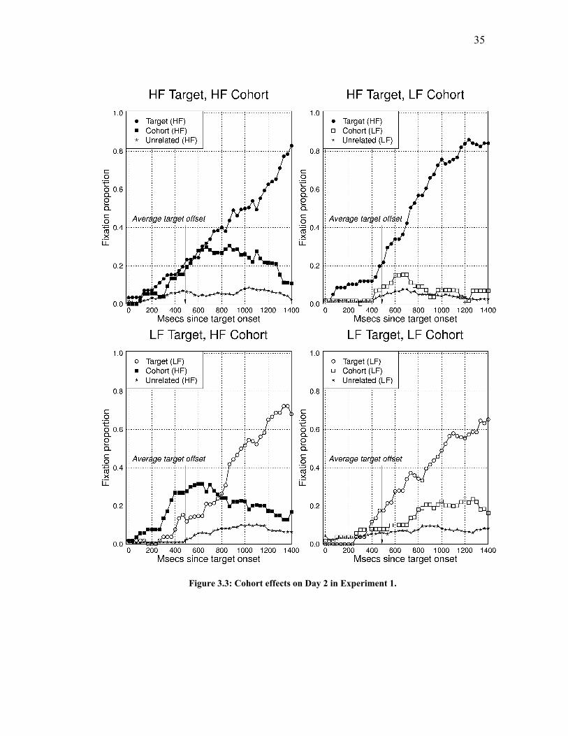
35
Figure 3.3: Cohort effects on Day 2 in Experiment 1.

36
Note that the slope of the target fixation probability (derived from a logistic
regression) was less than for real words (Day 1: probability increased .0006/msec;
Day 2: .0007; real words: .0021; see Figure 2.4 in Chapter 2), and the target
probability did not reach 1.0 even 1500 ms after the onset of the target name. Two
factors underlie this. First, the stimuli were longer than bisyllabic words like those
used by Allopenna et al. because of their CVCV structure. Second, although
participants were at ceiling on HF and LF items in the second test (Table 3.1), they
were apparently not as confident as we would expect them to be with real words, as
indicated by the fact that they made more eye movements than participants in
Allopenna et al. (1998): 3.4 per trial on Day 2 vs. 1.5 per trial for real words.
Table 3.1: Accuracy in training and testing in Experiment 1.
Session Overall HF LF
Training 1 (2AFC) 0.728 0.751 0.562
Training 4 (2AFC) 0.907 0.933 0.722
Training 7 (4AFC) 0.933 0.952 0.797
Day 1 Test 0.863 0.949 0.777
Training 8 (4AFC) 0.940 0.960 0.802
Training 11 (4AFC) 0.952 0.965 0.859
Training 14 (4AFC) 0.969 0.977 0.908
Day 2 Test 0.974 0.983 0.964

37
Figure 3.4: Rhyme effects on Day 2 in Experiment 1.
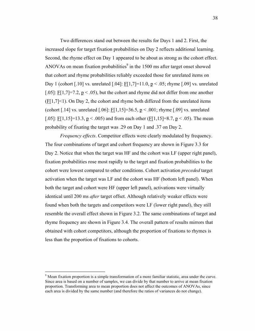
38
Two differences stand out between the results for Days 1 and 2. First, the
increased slope for target fixation probabilities on Day 2 reflects additional learning.
Second, the rhyme effect on Day 1 appeared to be about as strong as the cohort effect.
ANOVAs on mean fixation probabilities9 in the 1500 ms after target onset showed
that cohort and rhyme probabilities reliably exceeded those for unrelated items on
Day 1 (cohort [.10] vs. unrelated [.04]: F[1,7]=11.0, p < .05; rhyme [.09] vs. unrelated
[.05]: F[1,7]=7.2, p < .05), but the cohort and rhyme did not differ from one another
(F[1,7]<1). On Day 2, the cohort and rhyme both differed from the unrelated items
(cohort [.14] vs. unrelated [.06]: F[1,15]=36.5, p < .001; rhyme [.09] vs. unrelated
[.05]: F[1,15]=13.3, p < .005) and from each other (F[1,15]=8.7, p < .05). The mean
probability of fixating the target was .29 on Day 1 and .37 on Day 2.
Frequency effects. Competitor effects were clearly modulated by frequency.
The four combinations of target and cohort frequency are shown in Figure 3.3 for
Day 2. Notice that when the target was HF and the cohort was LF (upper right panel),
fixation probabilities rose most rapidly to the target and fixation probabilities to the
cohort were lowest compared to other conditions. Cohort activation preceded target
activation when the target was LF and the cohort was HF (bottom left panel). When
both the target and cohort were HF (upper left panel), activations were virtually
identical until 200 ms after target offset. Although relatively weaker effects were
found when both the targets and competitors were LF (lower right panel), they still
resemble the overall effect shown in Figure 3.2. The same combinations of target and
rhyme frequency are shown in Figure 3.4. The overall pattern of results mirrors that
obtained with cohort competitors, although the proportion of fixations to rhymes is
less than the proportion of fixations to cohorts.
9 Mean fixation proportion is a simple transformation of a more familiar statistic, area under the curve. Since area is based on a number of samples, we can divide by that number to arrive at mean fixation proportion. Transforming area to mean proportion does not affect the outcomes of ANOVAs, since each area is divided by the same number (and therefore the ratios of variances do not change).

39
Discussion
With relatively little training (98 exposures to HF items and 14 to LF items),
the time course of processing novel words became strikingly similar to that of real
words. In fact, after just 49 exposures to HF items and 7 exposures to LF items on the
first day of training, cohort and rhyme effects were already present. These results
from an artificial lexicon replicate previous results found with real words, including
the time course of frequency effects, as well as cohort and rhyme competition.
Moreover, they demonstrate that the artificial lexicon paradigm can be used
effectively to study the processing of newly-learned lexical items.
Experiment 2
The eye-tracking paradigm has two advantages over conventional
psycholinguistic measures: it provides a much finer-grained measure of lexical
processing in continuous speech, and it allows use of more naturalistic tasks than
response measures that require a metalinguistic judgment. However, a potential
limitation of the paradigm is the need for visual displays. This raises two concerns.
First, the paradigm might not be sensitive to effects of non-displayed lexical
competitors (which other methods, such as identification in noise or lexical decision,
are; Luce and Pisoni, 1998), making it difficult to examine effects of lexical
neighborhoods. Second, the observed effects might depend crucially on interactions
between pictured referents and names, rather than primarily reflecting input-driven
lexical activation.
Experiment 2 examines whether the neighborhood density effects observed in
Experiment 1 depend on the display of pictures of potential competitors. Experiment
2 asked the following question: will the frequency of an item's neighbors slow the
time course of recognition (as it does in tasks like identification in noise; e.g., Luce
and Pisoni, 1998) even when the neighbors are not displayed? We included the
cohort, rhyme, and frequency conditions from Experiment 1. In addition, we
compared the time course of recognition for HF and LF words with HF and LF
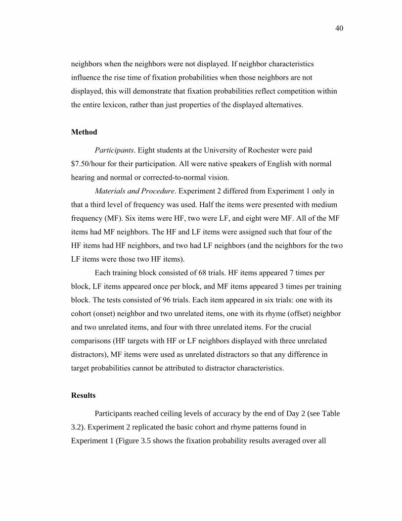
40
neighbors when the neighbors were not displayed. If neighbor characteristics
influence the rise time of fixation probabilities when those neighbors are not
displayed, this will demonstrate that fixation probabilities reflect competition within
the entire lexicon, rather than just properties of the displayed alternatives.
Method
Participants. Eight students at the University of Rochester were paid
$7.50/hour for their participation. All were native speakers of English with normal
hearing and normal or corrected-to-normal vision.
Materials and Procedure. Experiment 2 differed from Experiment 1 only in
that a third level of frequency was used. Half the items were presented with medium
frequency (MF). Six items were HF, two were LF, and eight were MF. All of the MF
items had MF neighbors. The HF and LF items were assigned such that four of the
HF items had HF neighbors, and two had LF neighbors (and the neighbors for the two
LF items were those two HF items).
Each training block consisted of 68 trials. HF items appeared 7 times per
block, LF items appeared once per block, and MF items appeared 3 times per training
block. The tests consisted of 96 trials. Each item appeared in six trials: one with its
cohort (onset) neighbor and two unrelated items, one with its rhyme (offset) neighbor
and two unrelated items, and four with three unrelated items. For the crucial
comparisons (HF targets with HF or LF neighbors displayed with three unrelated
distractors), MF items were used as unrelated distractors so that any difference in
target probabilities cannot be attributed to distractor characteristics.
Results
Participants reached ceiling levels of accuracy by the end of Day 2 (see Table
3.2). Experiment 2 replicated the basic cohort and rhyme patterns found in
Experiment 1 (Figure 3.5 shows the fixation probability results averaged over all
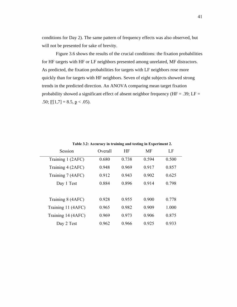
41
conditions for Day 2). The same pattern of frequency effects was also observed, but
will not be presented for sake of brevity.
Figure 3.6 shows the results of the crucial conditions: the fixation probabilities
for HF targets with HF or LF neighbors presented among unrelated, MF distractors.
As predicted, the fixation probabilities for targets with LF neighbors rose more
quickly than for targets with HF neighbors. Seven of eight subjects showed strong
trends in the predicted direction. An ANOVA comparing mean target fixation
probability showed a significant effect of absent neighbor frequency (HF = .39; LF =
.50; F[1,7] = 8.5, p < .05).
Table 3.2: Accuracy in training and testing in Experiment 2.
Session Overall HF MF LF
Training 1 (2AFC) 0.680 0.738 0.594 0.500
Training 4 (2AFC) 0.948 0.969 0.917 0.857
Training 7 (4AFC) 0.912 0.943 0.902 0.625
Day 1 Test 0.884 0.896 0.914 0.798
Training 8 (4AFC) 0.928 0.955 0.900 0.778
Training 11 (4AFC) 0.965 0.982 0.909 1.000
Training 14 (4AFC) 0.969 0.973 0.906 0.875
Day 2 Test 0.962 0.966 0.925 0.933

42
Figure 3.5: Combined cohort and rhyme conditions in Experiment 2.

43
Discussion
The results of Experiment 2 show that the eye-movement paradigm reveals
lexical processing that extends well beyond those items which are present in the
visual displays: the time course of recognition depended on characteristics of non-
displayed neighbors. The data in Figure 3.6 allow us to reject an alternative
interpretation of the results shown in Figure 3.3 and Figure 3.4, where target
probabilities rose most quickly when the target was HF and the neighbor was LF.
Fixations are serial, and competition among a set of simultaneously displayed items
might result from competition at a decision stage (e.g., motor programming). While
this problem diminishes with many observations, the current results provide strong
evidence for lexical competition rather than competition at fixation generation:
differences in target fixation probabilities were not accompanied by commensurate
differences in unrelated fixation probabilities (the weak trend [in HF condition =
.041; in LF condition = .038] was not reliable; F<1). Therefore, the differences shown
in Figure 3.6 indicate that more time was needed for the activation of the target to
become sufficiently large to generate initial eye movements when the target had HF
neighbors.
Discussion of Experiments 1 and 2
Experiments 1 and 2 demonstrate that after minimal training lexical
processing in a novel lexicon is strikingly similar to natural-language SWR. We
replicated several basic results from studies with real words: (a) the artificial lexical
items were processed incrementally, (b) phonetically similar neighbors become
partially activated with a time course that mapped onto emerging phonetic similarity,
and (c) recognition was affected by target and neighbor frequency. The current results
extended previous studies by showing that recognition depends on competition within
the lexicon: neighbor frequency affected processing even when neighbors were not
displayed.
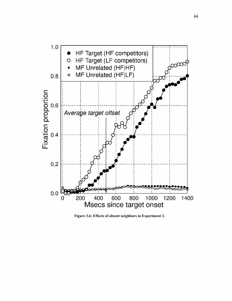
44
Figure 3.6: Effects of absent neighbors in Experiment 2.

45
A number of difficult issues arise in research with artificial languages,
including the nature of interactions with the native-language lexicon. These issues are
addressed in Experiments 3 and 4. Even before addressing those issues, however, the
present results demonstrate that research with a novel lexicon that builds upon an
existing phonological system can be used to evaluate the microstructure of spoken
language comprehension. This paradigm offers a valuable complement to more
traditional paradigms because it allows for (a) precise experimental control of the
distributional properties of the linguistic materials, (b) tests of distribution-based
learning hypotheses, and (c) evaluation of processing during early lexical learning.
Moreover, the use of artificial lexical items that refer to tangible objects, and
potential extensions to more complete artificial languages with well-defined
semantics, should make it possible to explore the interaction of distributional and
referential properties during language processing – issues that would be difficult to
address in research with non-referential artificial languages (due to the difficulty of
introducing semantic properties) or with natural language stimuli (due to lack of
precise control over distributional properties).
The Day 1 results from Experiment 1 also demonstrate that incremental
processing of multiple alternatives in parallel does not depend on highly (over-)
learned lexical representations. A difference observed between the tests on Days 1
and 2 is that while cohort effects were reliably stronger than rhyme effects on Day 2
(as Allopenna et al., 1998, found with real words), rhyme effects were as strong as
cohort effects on Day 1. This is consistent with Charles-Luce and Luce's (1990)
suggestion that children’s initial representations of words may depend more on
overall similarity than on sequential similarity. A more precise formulation is
suggested by simulations with simple recurrent networks (Magnuson, Tanenhaus, and
Aslin, 2000), in which rhyme effects are gradually weakened as a lexicon is learned
(and disappear when a lexicon is over-learned).

46
Chapter 4: Replication with English stimuli Experiment 3 is designed to replicate the basic neighborhood frequency effect
from Experiment 1using real English words. This is important because we need to
know that the effects we have observed with the artificial lexicons will generalize to
natural linguistic stimuli. We will test the recognition time for words that are high or
low frequency, crossed with high or low neighborhood density. Manipulating these
two factors allows the potential replication of the effects from Experiments 1 and 2.
In addition, the stimuli have high or low cohort densities. As we discussed in Chapter
2, Allopenna et al. (1998) found differential competition effects for items sharing
onsets (again, “cohorts”, since items overlapping at onset are predicted to compete by
the Cohort model) and rhymes.
While there was greater overlap between targets and rhymes in the Allopenna
et al. study than between targets and cohorts, cohorts competed more strongly than
rhymes (due, according to models like TRACE, to the temporal distribution of
similarity; a cohort’s initial overlap allows a head start relative to a rhyme’s later
overlap, with the result that rhymes are more strongly inhibited by cohorts of the
target and the target itself to reach high activation levels). The cohorts used by
Allopenna et al. would not, however, even count as neighbors under the
Neighborhood Activation Model. Cohorts mismatch by too many phonemes to be
counted as neighbors using the “shortcut” metric (neighbors differ by no more than
one phoneme substitution, addition or omission). Using the more sophisticated
metrics developed by Luce and colleagues, they would still be considered much less
likely competitors than rhymes. Rhymes have ceiling level positional confusion
probabilities (as an example of one phonemic similarity) at each phoneme where they
match the target, and low confusion probabilities only at onset. Cohorts have high
confusion probabilities beyond the first series of phones they share with the target,
and low confusion probabilities beyond. Typically, then, cohorts will have more
positions with low confusion probabilities. When the product of positional confusion

47
probabilities is computed, cohorts will have much lower predicted similarity than
rhymes.
This suggests two possible additions that could be made to Luce’s (1986; Luce
& Pisoni, 1999) neighborhood probability rule; first, similarity metrics perhaps
should be revised such that cohorts are considered neighbors, and second, early
positions perhaps should be given greater weight than later positions. Experiment 3
will tell us whether basic neighborhood effects can be observed with real words in the
visual world paradigm, and provide a first look at whether cohort information might
improve neighborhood metrics.
Experiment 3
Methods
Participants. Fifteen native speakers of English who reported normal or
corrected-to-normal vision and normal hearing were paid for their participation.
Stimuli. The target stimuli consisted of 128 imageable English nouns. There
were two levels (high and low) of frequency, neighborhood density, and cohort
density. There were 16 items in each of the 8 combinations of these levels (2 x 2 x 2).
After Luce and Pisoni (1998), neighborhood density was computed simply as the
summed log frequencies of all neighbors, including the target (note that this sum
forms the denominator of the frequency-weighted neighborhood probability rule;
since the numerator is the log frequency of the target, controlling for neighborhood
density entails equating summed neighbor log frequency). Neighbors were identified
using the 1-phoneme shortcut metric (items are considered neighbors if they differ by
a single phoneme addition, deletion, or substitution), which tends to be a better
predictor of recognition facility than more sophisticated metrics (Luce, personal
communication). Cohort density was the summed log frequencies of all items sharing
the same two-phoneme onset as the target (including the target itself). Table 4.1
shows the means and ranges of the two levels of each of these factors, and statistics
for individual items can be found in the Appendix.

48
Table 4.1: Frequencies and neighborhood and cohort densities in Experiment 3.
Low High
Mean Min Max Mean Min Max
Log frequency 2.3 .01 3.22 4.7 3.9 6.5
Neighborhood density 26.0 6.7 49.9 101.5 60.6 178.2
Cohort density 47.3 6.4 98.1 289.0 152.3 975.5
The auditory stimuli were produced by a male native speaker of English in a
sentence context (“Click on the chef.”). The stimuli were recorded using a Kay Lab
CSL 4000 with 16 bit resolution and a sampling rate of 22.025 kHz. The mean
duration of the “Click on the…” portion of the instruction was 427 ms. Mean target
duration was 551 ms.
The visual stimuli came from a variety of sources, including the Snodgrass
pictures (Snodgrass and Vanderwart, 1980), and a number of clip-art collections. We
tried to allow as little variability as possible in realism, style, and other
characteristics, but the large number of images required for this experiment made
perfect control untenable.10
Procedure. Trials were randomly ordered for each participant. On each trial,
the target and three distractors appeared after a 100 ms pause (during which the eye
tracker began recording) when the participant clicked on a central fixation square.
Concurrently, the auditory instruction began (e.g., “click on the yarn”). The trial
ended 150 ms after the participant clicked on one of the pictures.
The pictures were classified according to a handful of broad semantic classes
(e.g., person, animal, vehicle, appliance, tool). Only 1 item from each category was
permitted to appear in each display. The pictures were displayed approximately 2
degrees of visual angle from the central fixation square, at 45, 135, 225, and 315
10 We am currently collecting ratings of the pictures. Initial analyses based on a small number of
participants’ ratings indicate that there is almost no correlation between mean rating and
performance on the targets used in Experiment 3.
49
degrees relative to the central fixation square (i.e., in the corners of a square around
the central fixation square).
Eye movements were monitored using a SensorMotorics Instruments (SMI)
EyeLink eye tracker, which provided a record of point-of-gaze in screen coordinates
at a sampling rate of 250 hz. The auditory stimuli were presented binaurally through
headphones (Sennheiser HD-570) using standard Macintosh Power PC digital-to-
analog devices. Saccades and fixations were coded from the point-of-gaze data using
SMI’s software.
Predictions
The predictions for this experiment are straightforward. First, high-frequency
items should be recognized more quickly (as reflected in a steeper rise in target
fixation proportion beginning about 200 ms after noun onset) than low-frequency
items. Second, items with low neighborhood density should be recognized more
quickly than items in high-density neighborhoods, since the competitors in a dense
neighborhood (in aggregate) will compete more strongly than those in low density
neighborhoods. This would replicate the neighborhood effects found with real words
in previous studies (e.g., Luce and Pisoni, 1998), as well as the neighborhood density
effects in Experiments 1 and 2. Third, the same pattern (low-density < high-density)
should occur for cohort density, assuming items sharing onsets compete for
recognition. It is not clear how these factors should interact; we will examine this
post-hoc.
Results
Figure 4.1 shows the patterns for the main effects of frequency, neighborhood
density, and cohort density. As can be seen in the figure, the first and third predictions
appear to be borne out: fixation proportions rise more quickly for high-frequency
targets than low-frequency targets, and more quickly for items with low-density
cohorts than those in high-density cohorts. The pattern for neighborhood density is
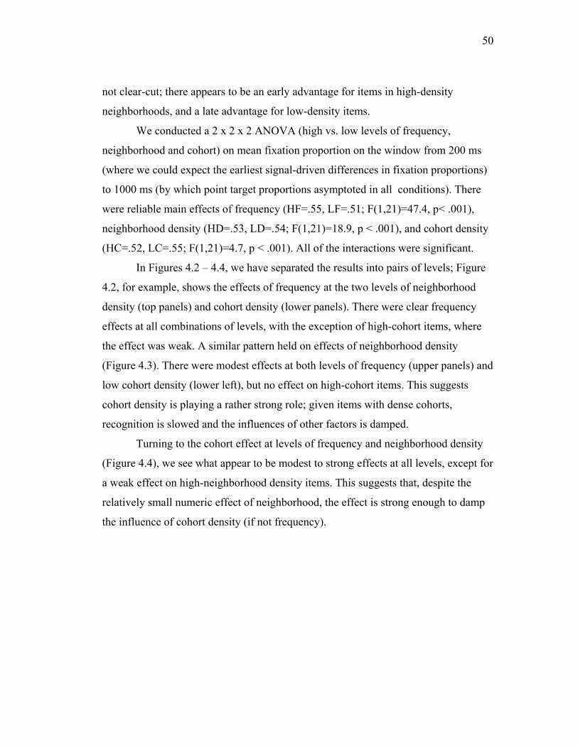
50
not clear-cut; there appears to be an early advantage for items in high-density
neighborhoods, and a late advantage for low-density items.
We conducted a 2 x 2 x 2 ANOVA (high vs. low levels of frequency,
neighborhood and cohort) on mean fixation proportion on the window from 200 ms
(where we could expect the earliest signal-driven differences in fixation proportions)
to 1000 ms (by which point target proportions asymptoted in all conditions). There
were reliable main effects of frequency (HF=.55, LF=.51; F(1,21)=47.4, p< .001),
neighborhood density (HD=.53, LD=.54; F(1,21)=18.9, p < .001), and cohort density
(HC=.52, LC=.55; F(1,21)=4.7, p < .001). All of the interactions were significant.
In Figures 4.2 – 4.4, we have separated the results into pairs of levels; Figure
4.2, for example, shows the effects of frequency at the two levels of neighborhood
density (top panels) and cohort density (lower panels). There were clear frequency
effects at all combinations of levels, with the exception of high-cohort items, where
the effect was weak. A similar pattern held on effects of neighborhood density
(Figure 4.3). There were modest effects at both levels of frequency (upper panels) and
low cohort density (lower left), but no effect on high-cohort items. This suggests
cohort density is playing a rather strong role; given items with dense cohorts,
recognition is slowed and the influences of other factors is damped.
Turning to the cohort effect at levels of frequency and neighborhood density
(Figure 4.4), we see what appear to be modest to strong effects at all levels, except for
a weak effect on high-neighborhood density items. This suggests that, despite the
relatively small numeric effect of neighborhood, the effect is strong enough to damp
the influence of cohort density (if not frequency).

51
Figure 4.1: Main effects in Experiment 3.

52
Figure 4.2: Interactions of frequency with neighborhood and cohort density.
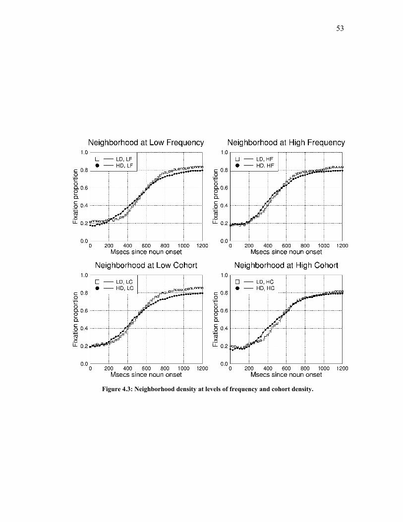
53
Figure 4.3: Neighborhood density at levels of frequency and cohort density.
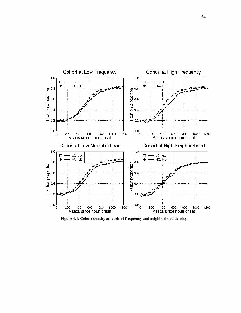
54
Figure 4.4: Cohort density at levels of frequency and neighborhood density.

55
Discussion
The current results replicate standard findings in spoken word recognition
(frequency and neighborhood density effects). They also confirm that words that
overlap in onset (initial consonant and vowel) – onset cohorts – have strong effects on
word recognition (as shown in Figure 4.1). The effect of cohort density is apparent
from the earliest signal-driven fixation proportions (around 200 ms after word onset),
but the advantage observed for items in low-density neighborhoods does not kick in
until about 600 ms after word onset. This is consistent with findings like those from
Allopenna et al. (1998) and Experiments 1 and 2, where we observe earlier, stronger
competition between targets and cohorts than between targets and rhymes. The cohort
density metric only takes into account words overlapping at onset, whereas
neighborhood density typically includes many items that are not cohorts, and
therefore, the overlap is temporally later. Consistent with this pattern, Newman et al.
(1997) found effects of neighborhood density on phoneme identification for
“medium” latency responses, but not for fast responses.
This suggests an explanation for the initial advantage for high-density items
(middle panel of Figure 4.1) and all levels of frequency and cohort density (Figure
4.3). An examination of the number of cohorts included in neighborhood density
reveals that a higher percentage of neighbors in low-density neighborhoods are also
cohorts; 58% of the neighbors in low-density neighborhoods are cohorts, versus 32%
in high density. Thus, low-density words are initially at a disadvantage because the
majority of their neighbors compete at onset. The low-density advantage shows up
later, when the majority (two thirds) of the neighbors in high-density neighborhoods
overlap substantially with the input (if one examines the tables in the Appendix, it is
clear that there is an interaction between neighborhood density and frequency in this
respect.
The implication for theories of spoken word recognition is that type of
competitor (where and how it mismatches a target) is important. We must develop

56
similarity metrics that take into account more directly the temporal aspect of
similarity among spoken words.
57
Chapter 5: Do newly learned and native lexicons interact?
While Experiments 1 and 2 demonstrated the feasibility of using artificial
lexicons to test specific hypotheses with precisely controlled stimuli, an important
control issue is whether the native lexicon influences recognition in an artificial
lexicon. If an artificial lexicon can be considered self-contained, design constraints
would be tremendously reduced. If the native lexicon does affect performance on
items in an artificial lexicon, one must take great care in designing artificial lexicons
to ensure that effects are not due to interactions with items in the participant’s native
lexicon.
The basis for the hypothesis that there ought to be interactions between
newly-learned and long-standing lexical representations is straight-forward.
Especially when the artificial lexicon is being presented in English carrier phrases
(e.g., “click on the pibu”), we might expect that the novel words are simply being
added to the native lexicon.
There are several possible bases for the opposite hypothesis. The artificial
lexicon might be functionally self-contained because it is a closed set. For example,
an initial disadvantage for low-frequency items dissipates when items are repeated in
an experiment (e.g., Scarborough et al., 1977). A possible explanation for closed set
effects, and an independent motivation for the “self-contained artificial lexicon”
hypothesis, is recency. The many recent presentations of the artificial items may boost
their saliency (potentially via, for example, enhanced resting level activation) such
that the representations of native lexical items are swamped.
If we fail to find effects of English neighborhood density on artificial lexical
items, we will not be able to distinguish between recency and closed-set explanations.
Our present purpose, however, is simply to determine how likely it is that effects
observed with artificial lexicons could be due to characteristics of the native lexicon.
In Experiment 4, we will test what influence the native lexicon has on a
learned artificial lexicon by creating novel words which, if they were English words,
58
would be in high- or low-density neighborhoods. Half would fall into high-density
neighborhoods, and half would fall into low-density neighborhoods. Half of the items
that would be in high-density neighborhoods and half that would be in low-density
neighborhoods will be high frequency within the artificial lexicon, and half will be
low frequency. If the newly-learned lexicon is self-contained, we should only observe
effects of the artificial lexicon's structure (i.e., a frequency effect). If the native
language lexicon influences recognition of the newly-learned lexicon, we should
observe an interaction of artificial and English lexical effects; e.g., if the artificial
lexical items are competing for recognition with English lexical items, low-frequency
words in the lexicon that would be in high-density English neighborhoods should be
harder to recognize than low-frequency artificial words that would be in low-density
English neighborhoods.
Experiment 4
Methods
Participants. Eight native speakers of English who reported normal or
corrected-to-normal vision and normal hearing were paid for their participation.
Participants attended sessions on two consecutive days. The sessions were both
between about 90 and 120 minutes long, and participants were paid $7.50 per hour.
Materials. The linguistic materials consisted of 20 artificial words formed by
taking low-frequency, low-cohort, high- and low-density words from the materials for
Experiment 3, and changing the final consonant. Thus, half of the resulting artificial
words would fall into high-density English neighborhoods, while the other half would
fall into low-density neighborhoods (see Table 5.111). The auditory stimuli were
produced by a male native speaker of English in a sentence context (“Click on the
yarp.”). The stimuli were recorded using a Kay Lab CSL 4000 with 16 bit resolution
11 Note that only low cohort items were used. The difference in mean cohort density between the high- and low-density items is small, given the variation in cohort density; for example, the mean cohort density for high-cohort density items in Experiment 3 was 289.
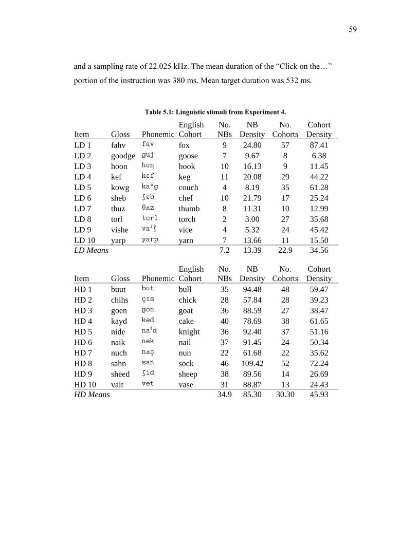
59
and a sampling rate of 22.025 kHz. The mean duration of the “Click on the…”
portion of the instruction was 380 ms. Mean target duration was 532 ms.
Table 5.1: Linguistic stimuli from Experiment 4.
Item Gloss PhonemicEnglish Cohort
No. NBs
NB Density
No. Cohorts
Cohort Density
LD 1 fahv fav fox 9 24.80 57 87.41 LD 2 goodge guj goose 7 9.67 8 6.38 LD 3 hoon hUn hook 10 16.13 9 11.45 LD 4 kef kEf keg 11 20.08 29 44.22 LD 5 kowg kaWg couch 4 8.19 35 61.28 LD 6 sheb SEb chef 10 21.79 17 25.24 LD 7 thuz T√z thumb 8 11.31 10 12.99 LD 8 torl tcrl torch 2 3.00 27 35.68 LD 9 vishe vaiS vice 4 5.32 24 45.42 LD 10 yarp yarp yarn 7 13.66 11 15.50 LD Means 7.2 13.39 22.9 34.56
Item Gloss PhonemicEnglish Cohort
No. NBs
NB Density
No. Cohorts
Cohort Density
HD 1 buut bUt bull 35 94.48 48 59.47 HD 2 chihs CIs chick 28 57.84 28 39.23 HD 3 goen gon goat 36 88.59 27 38.47 HD 4 kayd ked cake 40 78.69 38 61.65 HD 5 nide naid knight 36 92.40 37 51.16 HD 6 naik nek nail 37 91.45 24 50.34 HD 7 nuch n√C nun 22 61.68 22 35.62 HD 8 sahn san sock 46 109.42 52 72.24 HD 9 sheed Sid sheep 38 89.56 14 26.69 HD 10 vait vet vase 31 88.87 13 24.43 HD Means 34.9 85.30 30.30 45.93

60
The visual materials consisted of 20 unfamiliar shapes. These were
constructed by randomly filling 18 contiguous cells of a 6 x 6 grid. A distinctive set
was generated by creating 500 such figures, and randomly selecting twenty. Nine
examples are shown in Figure 5.1. Pilot tests indicated that these materials, while
clearly similar to those used in Experiments 1 and 2, were more distinctive and easier
to learn.
Figure 5.1: Examples of visual stimuli from Experiment 4.
Procedure. Participants were trained and tested in sessions on two consecutive
days. Each session lasted between 90 and 120 minutes. On day 1, participants were
trained with a two-alternative forced choice (2AFC) task for four blocks, then with
four-alternative forced choice (4AFC) for seven blocks. On day 2, training continued
with seven 4AFC blocks. At the end of each day, participants were given a 4AFC test
with no feedback. Eye movements were tracked during the testing session.
The structure of the training sessions was nearly identical to that used in
Experiments 1 and 2. First, a central fixation square appeared on the screen. The
participant then clicked on the square to begin the trial. After 100 ms, either two

61
shapes (in the first four training sessions) or four shapes (in the rest of the training
sessions and the tests) appeared (see Figure 3.1 for examples of displays in
Experiment 1). In contrast to Experiments 1 and 2, participants were not given
explicit instructions to fixate the central stimulus. When the participant clicked on the
fixation square, a 100 ms pause was followed by the appearance of the pictures and
the spoken instruction (e.g., “Click on the yarp.”). When participants responded, all of
the distractor shapes disappeared, leaving only the correct referent. The name of the
shape was then repeated. The object disappeared 200 ms later, and the participant
clicked on the square to begin the next trial. The testing session was identical to the
four-item training, except that no feedback was given (150 ms after the participant
clicked on an object, all of the pictures disappeared).
During training, half the items were presented with high frequency (HF), and
half with low frequency (LF). Frequency assignments were made randomly for each
participant. HF items were presented 6 times per training block, and LF items were
presented once per block, so there were 70 trials per training block. Each item was
presented six times in each test. For training and testing, distractors were chosen
randomly, except that in training, pictures corresponding to low-frequency items were
used as distractors more often than high-frequency pictures, in order to keep the
number of visual presentations of each picture comparable. Trials were presented in
random order, with the constraint that the same target could not occur on consecutive
trials.
During the tests, eye movements were monitored using a SensorMotorics
Instruments (SMI) EyeLink eye tracker, which provided a record of point-of-gaze in
screen coordinates at a sampling rate of 250 hz. The auditory stimuli were presented
binaurally through headphones (Sennheiser HD-570) using standard Macintosh
Power PC digital-to-analog devices. Saccades and fixations were coded from the
point-of-gaze data using SMI’s software.
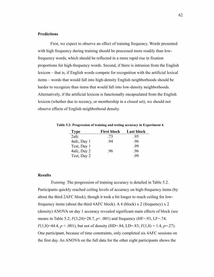
62
Predictions
First, we expect to observe an effect of training frequency. Words presented
with high frequency during training should be processed more readily than low-
frequency words, which should be reflected in a more rapid rise in fixation
proportions for high-frequency words. Second, if there is intrusion from the English
lexicon – that is, if English words compete for recognition with the artificial lexical
items – words that would fall into high-density English neighborhoods should be
harder to recognize than items that would fall into low-density neighborhoods.
Alternatively, if the artificial lexicon is functionally encapsulated from the English
lexicon (whether due to recency, or membership in a closed set), we should not
observe effects of English neighborhood density.
Table 5.2: Progression of training and testing accuracy in Experiment 4.
Type First block Last block 2afc .73 .95 4afc, Day 1 .94 .96 Test, Day 1 .99 4afc, Day 2 .96 .96 Test, Day 2 .99
Results
Training. The progression of training accuracy is detailed in Table 5.2.
Participants quickly reached ceiling levels of accuracy on high-frequency items (by
about the third 2AFC block), though it took a bit longer to reach ceiling for low-
frequency items (about the third 4AFC block). A 4 (block) x 2 (frequency) x 2
(density) ANOVA on day 1 accuracy revealed significant main effects of block (see
means in Table 5.2; F(3,24)=28.7, p< .001) and frequency (HF=.93, LF=.74;
F(1,8)=44.4, p < .001), but not of density (HD=.84, LD=.83; F(1,8) = 1.4, p=.27).
One participant, because of time constraints, only completed six 4AFC sessions on
the first day. An ANOVA on the full data for the other eight participants shows the
63
same pattern that was found in the day 1 2AFC sessions: there were significant effects
of block (F(6,42)=7.10, p < .001), frequency (HF=.99; LF=.96; F(1,7)=7.24, p <
.001), but not of density (F(1,7) = 0). A 2 (frequency) x 2 (density) ANOVA on the
data for all 9 participants also shows a main effect of frequency (HF=.99, LF=.96;
F(1,8)=32.50, p < .001), but not of density (HD=.97, LD=.98; F=.019). On day 2,
accuracy began at ceiling levels for both high- and low-frequency items and stayed
there. There were no effects of block, frequency or density. Thus, the training was
effective. Participants reached ceiling levels on the first day, and the training on day 2
served simply as practice.
Eye tracking tests. Participants reached ceiling levels of accuracy on both
day’s tests (accuracy > .99 in all conditions), such that there were significant accuracy
effects. Fixation probabilities over time are plotted for the six crucial comparisons in
Figure 5.2 (frequency effects on both days) and Figure 5.3 (density effects on both
days). The top two panels plot the main effects of frequency and frequency within
high- and low-density items (Figure 5.2) and the analogous density effects (Figure
5.3). Note that on both days, the frequency effect apparent in the top left panels is due
to the relatively strong frequency effect for high-density items (middle panels of
Figure 5.2). Despite the absence of an apparent effect of density in the top panels of
Figure 5.3, there was a strong trend among low-frequency items (bottom panels).
Thus, these summary plots suggest an effect of frequency only on high-density items,
and an effect of density only on low-frequency items.
We conducted analyses of variance on mean fixation proportions (as in the
previous experiments) in the window from 200 ms (when we would expect the
earliest signal-driven differences in fixation proportions) to 1400 ms (approximately
where target fixation proportions asymptote in each condition). We conducted
identical analyses on the data from both days. The trends were identical on both days,
so we will only report the results for day 2.
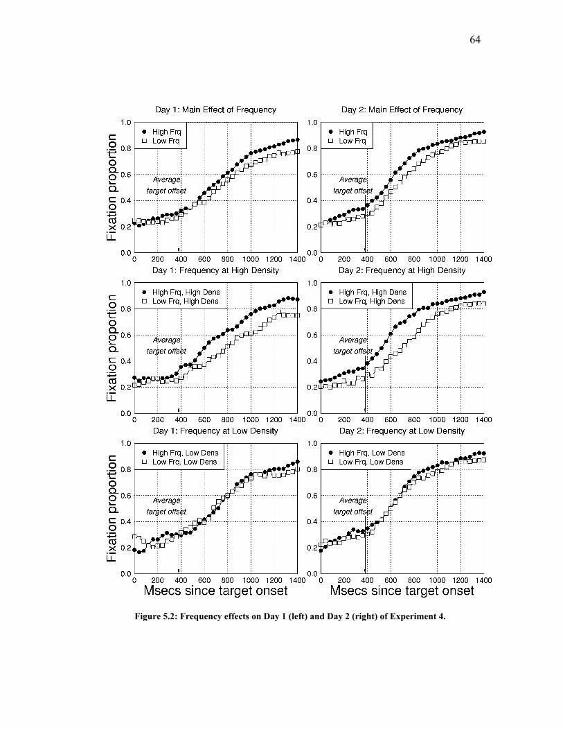
64
Figure 5.2: Frequency effects on Day 1 (left) and Day 2 (right) of Experiment 4.
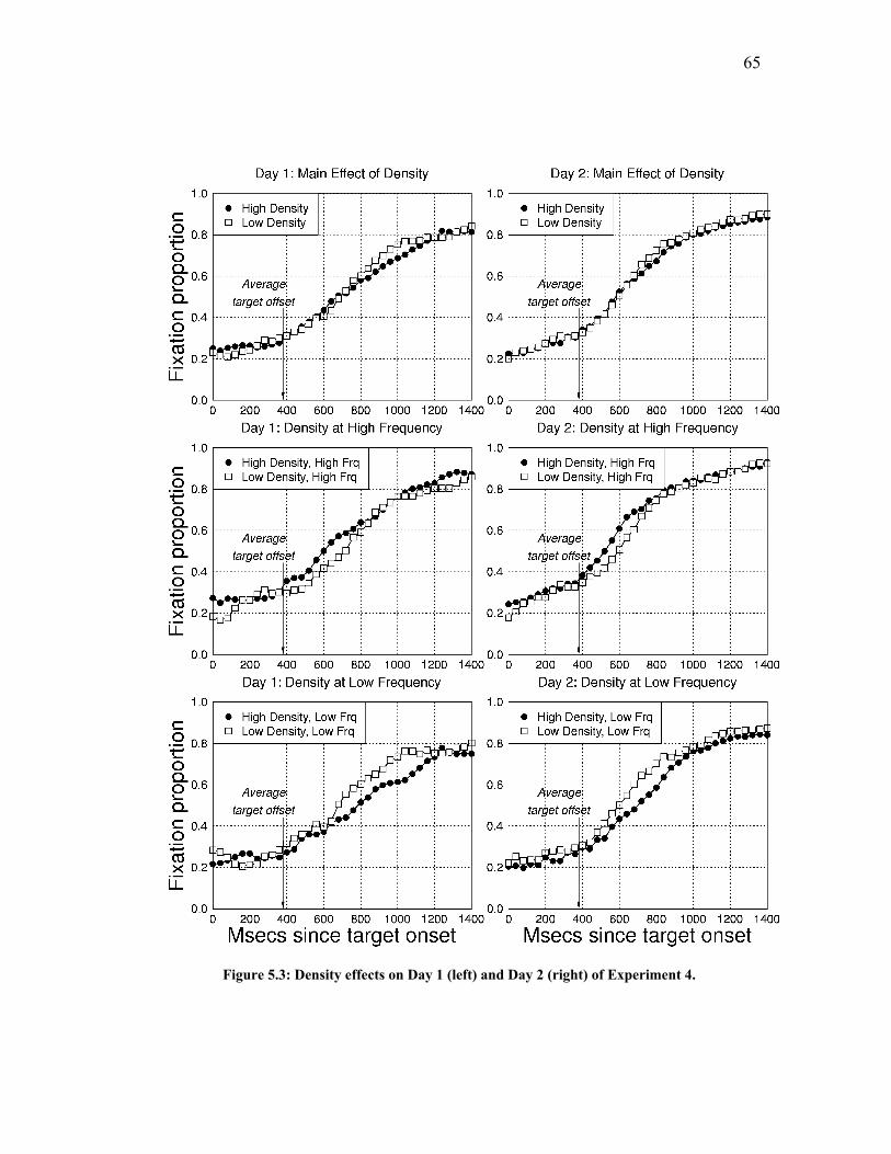
65
Figure 5.3: Density effects on Day 1 (left) and Day 2 (right) of Experiment 4.
66
We conducted a 2 (high- vs. low frequency) x 2 (high vs. low density)
ANOVA. There was a significant main effect of frequency (HF=.67, LF=.59;
F(1,7)=24.6, p = .002; effect size = .72), but not of density (although the trend was in
the expected direction, i.e., lower-density items were fixated more: HD=.62, LD=.64;
F(1,7)=.6). Planned comparisons of the frequency effect at the two levels of density
confirm the pattern shown in Figure 5.2: there was a reliable frequency effect on
high-density items (HF=.68, LF=.57; F(1,7)=18.8, p = .003), and a non-significant
trend for low-density items (HF=.65, LF=.62; F(1,7)=1.5, p=.266). We conducted
planned comparisons on density at the two levels of frequency, despite the apparent
reversal in the density effect on high-frequency items. The reversal at high frequency
was not reliable (HD=.68, LD=.65; F(1,7) = 1.3, p = .29), nor was the predicted trend
on low-frequency items (HD=.57, LD=.62; F(1,7)=2.6, p=.15).
Discussion
The main effects from the eye-tracking test conform to one set of predictions
for this experiment. There was a significant effect of the experimental frequency
manipulation, but not of English neighborhood density. This suggests that an artificial
lexicon can be considered functionally isolated from a participant’s native lexicon.
While we cannot distinguish between the two possible bases discussed earlier for this
pattern (closed-set vs. recency), the purpose of Experiment 4 was simpler. We wished
to test whether characteristics of the native lexicon impinge on an artificial one in
experiments such as Experiments 1 and 2. Again, the main effects of Experiment 4
indicate that the native lexicon does not impinge on an artificial lexicon.
The interactions, however, are puzzling, and hint at a more complex story. It
is important to note that the basis for the frequency effect is in high-density items, and
that the pattern is largely consistent across participants. An examination of individual
participant data (for day 2) shows that seven of eight participants show a frequency
trend on high-density items. Only two show predicted (HF > LF) frequency trends on
67
low-density items, with four others showing no apparent trend, and two showing
moderate reversals (LF > HF) on low-density items. Conversely, five participants
show moderate to strong density trends (LD > HD) on low-frequency items, while
two show no apparent trend, and one an apparent reversal (HD > LD). Only one
shows a trend in the expected direction (LD > HD) on high-frequency items, with
four showing no apparent trend, and three showing apparent reversals (HD > LD).
To summarize the pattern, there are effects of frequency (more-or-less only)
on high-density items. Although density trends do not reach significance at either
high or low levels of frequency, the patterns in the individual data suggest that the
trend towards a low-density advantage on low-frequency items might prove reliable
with perhaps twice as many participants (the effect size is .17, which falls into
Cohen’s [1977] “large” category). What can explain this odd pattern? If anything, we
might expect to find stronger frequency effects on low-density items, where the
influence of the English lexicon ought to be weaker.
The statistics reported in Table 5.1: Linguistic stimuli from Experiment 4.
suggest one possible confound in the items. Although the range of English cohort
densities is small given the possible range (see Experiment 3), one could easily divide
each set into relatively high- and low-cohort density items. We did this by rank
ordering the high and low neighborhood density items by cohort density, and labeling
the five in each group with the highest cohort densities as such. An ANOVA with the
added factor of cohort density did not reveal any influence of cohort density; there
was not a main effect of cohort density, nor any interactions with frequency or
neighborhood density. Another way to assign items to cohort density groups would be
to rank order them without regard to neighborhood density (since, for example, some
high-neighborhood/“low-cohort” items would have higher cohort density than some
low-neighborhood/“high-cohort” items). We ran the analysis again with items
assigned to cohort group simply by their rank-ordered cohort density. Again, there
was not a main effect of cohort density, nor any interactions of cohort density with

68
frequency or neighborhood density. Thus, cohort density cannot explain the pattern of
results.
Some differences in the current procedures and results compared to those of
Experiments 1 and 2 suggest another possibility. Participants seemed to learn faster
with the current materials than with those used in Experiments 1 and 2 (compare
Table 3.1, Table 3.2, and Table 5.2). We suspect that the visual stimuli account for
much of the difference. The visual stimuli for Experiment 4 were more complex than
those for Experiments 1 and 2 (being created by filling 18 cells in a 6 x 6 grid, rather
than 8 cells in a 5 x 5 grid), which seemed to make them more discriminable. The
high:low frequency ratio was 6:1 in this experiment, as opposed to 7:1 in the earlier
ones. Also, each item was repeated 6 times in the test. Any of these three things (or
their combination) might have weakened the effect of the frequency manipulation. A
frequency effect might diminish given more salient and therefore better-learned
stimuli when participants have practiced on the items at ceiling levels of performance
for an extended period. The 7:1 ratio used in the earlier studies might have been close
to the minimum needed to achieve robust frequency effects in the artificial lexicon
paradigm. Similarly, repeated exposures in the test could weaken frequency.
Why should ceiling level performance result in the non-intuitive frequency
effect only on high-density items? It is possible that when the frequency effect is
diminished, for whatever reason, the task has become too easy. For example, if we
were to add a cognitive load manipulation or noise to the stimuli, we might see a
stronger frequency effect on all items.
Density may be playing a role akin to the role of noise. The high-density items
may be more difficult to process, but not so much so that we find a main effect of
density (again, because participants are at ceiling levels of performance). The result is
that the slight added difficulty allows a slightly more sensitive measure of frequency,
and we observe robust frequency effects on high-density items. Conversely,
frequency may play the same role for density. The low-frequency items are more
difficult to process, since they are not learned as well as the high-frequency items
69
(despite ceiling-level performance), and thus allow a more sensitive measure of
density (with the strong LD > HD trend observed for low-frequency items).
However, if we examine the percentage of neighbors at the different levels
that are also cohorts (as we did for the preceding experiment), we find another
explanation for the trend towards the predicted neighborhood effect on low-frequency
items but not on high-frequency items: 60% of high-frequency, low-neighborhood
density items are also cohorts, compared to 31.5% of high-frequency, high-
neighborhood density items. Again, this would predict an initial disadvantage for
low-density items, since most of their neighbors will be active at word onset.
However, the same pattern holds (albeit more weakly) for low-frequency items, so
this account may be incorrect.
Conclusion
To conclude, what are the implications for artificial lexicon studies? To a first
approximation, the statistically reliable results of Experiment 4 suggest that items in
an artificial lexicon – in the paradigm described in Experiments 1, 2 and 4 – can be
considered functionally isolated from a participant’s native lexicon. The non-
significant interactions between artificial lexicon frequency and English density,
though, suggest that caution is in order; Experiment 4 cannot be interpreted as
suggesting there are no interactions between artificial and native lexicons. The
density manipulation may not have been strong enough, although it was nearly as
strong as it could be given that we had to constrain the materials to highly imageable
nouns. On the other hand, the materials used in Experiment 4 may represent a worst-
case scenario. The items were designed to be highly similar to English words, yet we
did not observe reliable differences due to English density. While experimenters
ought to be wary of interactions with native lexicons when using artificial lexicons,
and explicitly measure factors such as the density, the results of Experiment 4 suggest
that it may well be difficult to find native-lexicon interactions even when an
experiment is biased to find them.

70
Chapter 6: Top-down constraints on word recognition A central issue in the language processing research in the last few decades has
been modularity, in terms of division of labor in the language processing system via
distinct processing stages or levels of representation (such as word recognition,
syntactic and semantic processing; e.g., Fodor, 1983; see Gaskell and Marslen-
Wilson, 1997, for arguments for a rather minimal number of levels), the degree to
which information is shared between such theoretical levels (e.g., Tanenhaus et al.,
1979), or how information flows within a level (e.g., Elman and McClelland, 1988;
Norris, McQueen and Cutler, 2000; Samuel, 1981). Arguments for strong modularity
(discrete divisions between and within sensory systems, and information
encapsulation within systems) run along the following lines: keeping information
sources separate at initial stages of processing will make a system more efficient and
less prone to hallucinations induced by top-down influences in the absence of robust
bottom-up information. Arguments for interaction are based on the notion that a
system can be made more efficient by allowing any sufficiently predictive information
source to be integrated with processing as soon as it is relevant.
Experiment 5 explores to what degree lexical activation is independent from
other aspects of language processing. This issue has been explored many times
previously. The seminal results on this topic were reported by Tanenhaus et al. (1979)
and Swinney (1979). Tanenhaus et al. presented participants with spoken sentences
that ended with a syntactically ambiguous word (e.g., “they all rose” vs. “they bought
a rose”). If participants were asked to name a visual target immediately at the offset
of the ambiguous word, priming was found both for the alternative suggested by the
context (e.g., “stood” given “they all rose”) and for homophones that would not fit the
syntactic frame (e.g., “flower”). Given a 200-ms delay prior to the presentation of the
visual stimulus, only the syntactically appropriate word was primed. This suggests
that while top-down information such as syntactic expectations influence word
recognition, bottom-up information prevails in the earliest moments of word

71
recognition, and top-down information comes into play as a relatively late-acting
constraint. Tanenhaus et al. argued that this made sense in terms of the predictive
power of a form-class expectation. Knowing that the next word will be one of tens of
thousands of nouns, for instance, would afford virtually no advantage for most nouns
(those without homophones in different form classes). Furthermore, expectations for
classes like noun or verb might be very weak because modifiers can almost always be
inserted before either class (e.g., “they just rose”, “they bought a very pretty red
rose”; cf. Shillcock and Bard, 1993).
Tanenhaus and Lucas (1987) interpreted this delayed top-down result in the
context of evidence for feedback within word recognition. Elman and McClelland
(1988), Ganong (1980) and Samuel (e.g., 1981), for example, provided evidence
supporting strong lexical effects on phonemic perception. Tanenhaus and Lucas noted
that in cases where there were early effects of top-down information sources, a part-
whole relationship existed. For example, phonemes (presumably) form part of the
representation of words, whereas the relationship between words and form classes is
one of set membership. Tanenhaus and Lucas speculated that one might find top-
down effects in cases where there is a part-whole relationship between words and
some larger unit, such as an idiomatic phrase.
Shillcock and Bard (1993) pointed out that there are form classes which are
more predictive than noun or verb, simply because the number of members in the set
is much smaller: closed-class words. They examined whether /wUd/ in a sentence
context favoring the closed-class item, “would” (e.g., “John said that he didn’t want
to do the job, but his brother would, as we later found out”) would prime associates of
its homophone, “wood”, such as “timber” (and vice-versa, given a context like “John
said he didn’t want to do the job with his brother’s wood, as we later found out”).
They found priming for “timber” given the open-class context (favoring “wood”)
immediately after the offset of /wUd/, but not given the closed-class context. The
same result held when they probed half-way through the pronunciation of /wUd/. This

72
suggests that the closed-class context was indeed sufficiently constraining to bias
even the earliest moments of word recognition. A cloze test (in which participants
were asked to supply the next word given the sentence contexts up to the word just
prior to “would” or “wood”, with the understanding that the word they supplied
would not be the last in the sentence) confirmed that the closed-class context was
much more predictive. While participants provided words of the same form class as
the target most of the time for both cases (74% for closed-class, 85% for open), they
were much more likely to provide the target given the closed-class context (34.4%)
than the open-class context (1.3%).
This result is consistent with the view that top-down information sources will
be integrated early in processing when they are sufficiently predictive. In Experiment
5, we tested the hypothesis that even form class expectations for open-class words
could constrain word recognition given a context with sufficient predictive power.
We used an extension of the artificial lexicon paradigm. Participants learned the
names of shapes – the nouns of the artificial lexicon – as well as the names of textures
that could be applied to the shapes – the adjectives. Instructions were given in an
English context, with English word order (e.g., “click on the /pib√/ [adj] /tedu/
[noun]”). The lexicon contained phonemic cohorts (e.g., /pibo/ and /pib√/) that
come from different syntactic categories (e.g., /pibo/ was a noun and /pib√/ was an
adjective) or the same category (e.g., another noun was /pibe/). While it would be
possible to conduct the experiment with English items (e.g., “purple” and “purse”),
we could not achieve the same level of consistency across items in terms of the
relationships between nouns and adjectives.
We created conditions in which the visual context provided strong syntactic
expectations by constructing contexts in which adjectives were required (e.g., two
examples of the shape associated with /pibo/, but with two different textures) or
infelicitous (e.g., two different shapes, making the adjective superfluous, even if the
shapes have different textures). If syntactic expectations in conjunction with
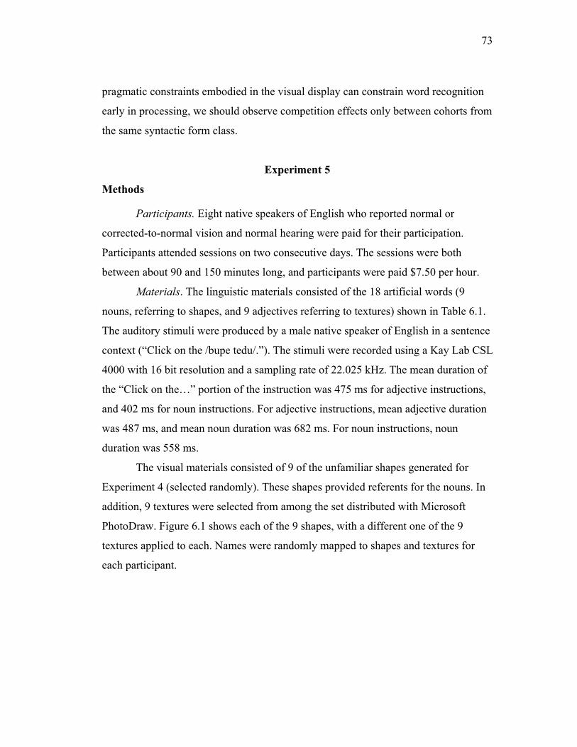
73
pragmatic constraints embodied in the visual display can constrain word recognition
early in processing, we should observe competition effects only between cohorts from
the same syntactic form class.
Experiment 5
Methods
Participants. Eight native speakers of English who reported normal or
corrected-to-normal vision and normal hearing were paid for their participation.
Participants attended sessions on two consecutive days. The sessions were both
between about 90 and 150 minutes long, and participants were paid $7.50 per hour.
Materials. The linguistic materials consisted of the 18 artificial words (9
nouns, referring to shapes, and 9 adjectives referring to textures) shown in Table 6.1.
The auditory stimuli were produced by a male native speaker of English in a sentence
context (“Click on the /bupe tedu/.”). The stimuli were recorded using a Kay Lab CSL
4000 with 16 bit resolution and a sampling rate of 22.025 kHz. The mean duration of
the “Click on the…” portion of the instruction was 475 ms for adjective instructions,
and 402 ms for noun instructions. For adjective instructions, mean adjective duration
was 487 ms, and mean noun duration was 682 ms. For noun instructions, noun
duration was 558 ms.
The visual materials consisted of 9 of the unfamiliar shapes generated for
Experiment 4 (selected randomly). These shapes provided referents for the nouns. In
addition, 9 textures were selected from among the set distributed with Microsoft
PhotoDraw. Figure 6.1 shows each of the 9 shapes, with a different one of the 9
textures applied to each. Names were randomly mapped to shapes and textures for
each participant.

74
Table 6.1: Artificial lexicon used in Experiment 5.
NOUN (shape) ADJ (texture) 1 pibo pib√ 1 2 pibe 3 bupo bup√ 2 bupe 3
4 tedu tedi 4 tedE 5
5 dotE doti 6 6 dotu 7 kagQ kagai 7 kagU 8
8 gawkU gawkQ 9 9 gawkai
Figure 6.1: The 9 shapes and 9 textures used in Experiment 5.
75
Procedure. Participants were trained and tested in sessions on two consecutive
days. Each session lasted between 90 and 120 minutes. On day 1, participants were
trained first on the nouns in a two-alternative forced choice (2AFC) task (with no
texture, i.e., solid black). As in previous experiments, two shapes would appear, the
participant would hear an instruction to click on one (e.g., “click on the bupo”), and
when they clicked, one item would disappear, leaving the correct item on the screen,
and its name was repeated. There were 14 repetitions of each item, split into 3 blocks
of 48 trials. Items were not repeated on consecutive trials, and were ordered such that
every item was repeated 7 times every 72 trials. Following the 2AFC blocks, noun
training continued with 3 blocks of 4AFC, with identical ordering constraints and
numbers of trials. Each shape appeared equally often as distractors.
Adjective training then began. First, participants saw two exemplars of one
shape, with different textures. They heard an instruction, such as “click on the bupe
pibo”. Since they already knew that, e.g., “pibo” referred to one of the shapes,
participants found it transparent that “bupe” referred one of the textures. As in the
noun training, after they clicked on one item, the incorrect one disappeared and the
full name was repeated. Each adjective and each noun were targets on 8 trials in each
block; each adjective was randomly paired with 8 different nouns in each block. After
three 48-trial 2AFC blocks, there were three 4AFC blocks, with four exemplars of the
same shape with four different textures. These were followed by three more blocks of
4AFC, but with two exemplars each of two shapes, each with a different texture
(requiring participants to recognize both the adjective and noun).
After this, a more complex training regime began. On some trials, four
different shapes appeared. On others, two pairs of shapes appeared. On every trial,
each shape had a different texture. On trials with two pairs of shapes, an adjective
was required to make unambiguous reference, and the full referent was specified on
such trials (e.g., “click on the bupe pibo”). On trials with four different shapes, the
adjective was not required – each item could be identified unambiguously by the
name of the shape, and so only the noun was specified in the instruction (e.g., “click

76
on the pibo”). In fact, using the adjective would be infelicitous, on Grice’s (1975)
maxim of quantity (one should not over-specify, which is in fact the observed
tendency in natural conversation). Each adjective was repeated 8 times in every block
of 144 trials, paired each time with a different, randomly selected noun. Each noun
was repeated as the target item 8 times in the 4-noun trials. Trials were presented in
blocks of 48. Participants completed 3 blocks of this mixed training on day 1. On day
2, they completed 12 more, which comprised the entire training phase on day 2.
After each 48-trial presentation block, the participant saw a summary of his or
her accuracy in that block. To motivate participants, we told them that each training
segment would continue until they reached 100% accuracy. Typically, we moved to
each successive training phase after the number of blocks listed above for each
segment, except in a few rare cases where participants were below 90% accuracy
after the specified number of blocks, in which case training continued for another 1-2
blocks.
Each day ended with a 4AFC test with no feedback. We tracked participants’
eye movements during the test. There were six basic conditions in the test. In the
noun baseline condition, there were four different shapes, and no shape nor adjective
was a competitor of the target noun. In the noun plus noun cohort condition, there
were four shapes, and one of them was a cohort to the target (e.g., the target might be
/pibo/, and /pibe/ would also be displayed), but no shape had the target’s adjective
cohort texture applied (e.g., no shape would have the /pib√/ texture). In the noun plus
adjective cohort condition, four different shapes were displayed. The noun cohort was
not displayed, but the adjective cohort was (e.g., a distractor might be /pib√ tedu/).
In these conditions, the instruction would only refer to the noun (e.g., “click on the
pibo”).
In the other three conditions, two exemplars of two different shapes were
displayed, requiring the adjective to be used in the instruction. In the adjective
baseline condition, none of the distractor textures were cohorts of the target, and
neither were any of the nouns. In the adjective plus adjective cohort condition, one of
77
the non-target textures was a cohort to the target (e.g., the target might be
/tedi dotu/, and one non-target might be /tedE bupo/), but no noun cohorts of the
target would be displayed. In the adjective plus noun cohort condition, none of the
distractors would have textures that were cohorts to the target texture, but a noun
cohort would be displayed (e.g., given /tedi dotu/ as the target, /bupe tedu/ might
be included).
The following scheme was used to ensure that each adjective and target
appeared equally often as targets in the test. Note that nouns and adjectives can be
divided into two sets: items with two cohorts in the same form class and one in the
other, or vice-versa. Nouns with noun cohorts appeared in six noun baseline trials,
two noun plus noun cohort trials (once with each cohort), and once in the noun plus
adjective cohort condition (with their one adjective cohort). Nouns with two adjective
cohorts appeared in 7 noun baseline trials, 0 noun cohort trials, and two noun plus
adjective cohort trials. The same pattern was used with adjective conditions:
adjectives with adjective cohorts appeared in 6 adjective baseline trials, those with
noun cohorts appeared in 7; items with adjective cohorts appeared in one adjective
plus adjective cohort trial with each cohort; items appeared one time with each of
their one or two noun cohorts. Note that since, for example, nouns with two adjective
cohorts and no noun cohort would appear in two adjective plus noun cohort trials,
each noun appeared in the same number of trials.
The total number of trials in the test was 162. There were 57 adjective
baseline trials: (3 [adjectives without adjective cohorts] x 7 repetitions) + (6
[adjectives with adjective cohorts] x 6 repetitions); 57 noun baseline trials (3 [nouns
without noun cohorts] x 7 repetitions) + (6 [nouns with noun cohorts] x 6 repetitions);
12 adjective with adjective cohort trials (6 x 2 repetitions); 12 adjective plus noun
cohort trials: (3 [adjectives without adjective cohorts] x 2) + (6 [adjectives with
adjective cohorts] x 1); 12 noun with noun cohort trials (6 x 2 repetitions); and 12
noun plus noun adjective trials: (3 [nouns without noun cohorts] x 2) + (6 [nouns with
noun cohorts] x 1).

78
During the tests, eye movements were monitored using a SensorMotorics
Instruments (SMI) EyeLink eye tracker, which provided a record of point-of-gaze in
screen coordinates at a sampling rate of 250 hz. The auditory stimuli were presented
binaurally through headphones (Sennheiser HD-570) using standard Macintosh
Power PC digital-to-analog devices. Saccades and fixations were coded from the
point-of-gaze data using SMI’s software.
Predictions
The conditions in this experiment are numerous and complex enough to
warrant a careful review of the predictions. In the noun baseline condition, we would
expect people to be equally likely to fixate the target and any distractor at the onset of
the noun, with a gradual shift towards the target after about 200 ms. In the noun plus
noun cohort condition, we would expect equal fixation proportions to the target,
cohort, and distractors at noun onset, followed by a gradual increase to the target and
cohort about 200 ms after onset, and then a final shift to the target a few hundred ms
later (once disambiguating phonetic information is encountered). There are two
possible predictions for the noun plus adjective cohort condition. First, if initial
processing is encapsulated (and thus only operates on bottom-up information), we
should see a cohort effect like the one predicted for the noun plus noun cohort
condition. This is the prediction if discourse constraints provided by the visual
display coupled with syntactic expectations cannot prevent activation of items from
irrelevant form classes. Second, if those constraints can influence the early stages of
word recognition, we should not see a cohort effect when the cohort is from a
different form class. The predictions for the three adjective conditions parallel these,
although the timing will be different, since participants must recognize the noun
before they can select the target.

79
Results
Two participants failed to reach ceiling levels of accuracy (they performed at
less than 90% correct on the test on day 2). The data of these two participants was
excluded from the analyses.
Training. The progression of accuracy at key points during training and
testing is detailed in Table 6.2.
Table 6.2: Progression of accuracy in Experiment 5.
Type First block Last block
2 noun .70 .96
4 noun .93 .97
4 adjectives, 1 noun .88 .96
4 adjectives, 2 nouns .97 .98
Mixed, Day 1 .96 .96
Test, Day 1 .98
Mixed, Day 2 .96 .96
Test, Day 2 .98 .98
Test. The results from the test on day 2 are shown in Figure 6.2 (critical noun
conditions) and Figure 6.3 (critical adjective conditions). Examples of possible
stimulus items are shown to the left of each panel of each figure (these would be
arranged around the central fixation cross in an actual experimental display). Note
that in the cross-form class conditions (noun with adjective cohorts and adjective with
noun cohorts) there were two cohorts in the display. This was necessary in the case of
the adjective plus noun cohort condition; in order for the display to demand that an
adjective be used, two exemplars of two different shapes had to be displayed. To
make the noun plus adjective cohort condition comparable, two items were displayed
with textures whose names were cohorts to the noun target.

80
Figure 6.2: Critical noun conditions in Experiment 5.
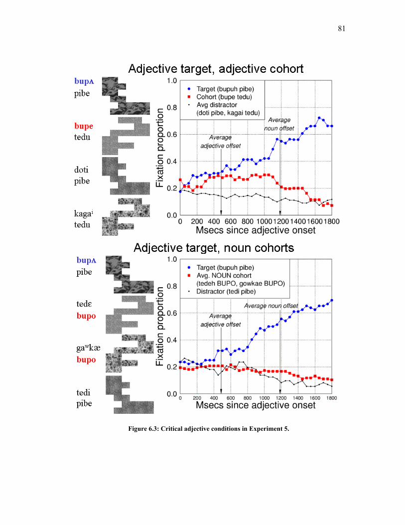
81
Figure 6.3: Critical adjective conditions in Experiment 5.
82
The results are consistent with a non-encapsulated word recognition system.
Compare the upper and lower panels of the two figures. While strong cohort effects
are apparent in the upper panels (the within-form class competitor conditions), there
do not appear to be cohort effects in the lower panels (between-form class
conditions). Analyses of variance on mean fixation proportion in the noun conditions
over the window from 200 ms (where we first expect to see signal-driven fixations) to
1400 ms (where the target proportions asymptote) confirm the trends. There was a
reliably greater proportion of fixations to the cohort than to the distractors in the noun
plus noun cohort condition (cohort = .25, mean distractor = .12; F(1, 11)=10.16, p =
.009), but not in the noun plus adjective cohort condition (cohort = .15, mean
distractor = .15; p = .89). The same was true for the adjective conditions, over the
window from 200 to 1800 (the window was extended because of the longer lag prior
to disambiguation). There were reliably more fixations to the cohort in the adjective
plus adjective cohort condition (cohort = .22, mean distractor = .15; F(1,11)=7.2, p =
.02), but not in the adjective plus noun cohort condition (cohort = .16, mean distractor
= .15, p = .59).
Discussion
The results are consistent with the hypothesis that top-down constraints are
integrated early in processing when they are highly-predictive. Phonemically similar
items competed only when there were from the same form class. This suggests that,
contra strong modularity, relative activation can be constrained given a highly
informative context. There are two caveats which must be mentioned.
First, we have not demonstrated that the nouns and adjectives would compete
in the absence of pragmatic constraints feeding syntactic expectations. For example,
given a display containing a /tedi pibo/, a /dotu gawkai/, and two /bupo/s – a
/pib√ bupo/ and a /kagU bupo/ – the first two items could be referred to just
with the appropriate noun, whereas the latter two require the adjective to be specified.

83
If the target were /pib√/ or /pib√ bupo/, those two items should compete due to
their initial overlap and the absence of pragmatic/syntactic constraints. It is possible
that in the context of the artificial lexicon, nouns and adjectives would not compete
even under these circumstances, although it is difficult to conceive of a mechanism
which would predict this.
Second, this effect depends on the closed-set nature of the lexicon. That is,
participants know that the targets will only be drawn from the small set of items they
have heard repeated for hours. Word recognition presumably is occurring with
activation and competition among the items in the lexicon, with no or minimal
interference from the English lexicon (see Experiment 4). It is possible that the effect
would not generalize to real words because the relative strength of the constraint
would be weakened; instead of aiding in selecting among 18 words, the constraint
would have to help select from tens of thousands. We could test this by using a larger
artificial lexicon, or even better, by replicating this result using English stimuli.
A potential concern based on these two caveats is that this result demonstrates
a central role for the visual display, whereas Experiment 2 was devoted to showing
that we can detect differences in activation due to non-displayed competitors, that is,
that the display does not constrain processing to the visible items. The current result
does not demonstrate that the visual display determines which items can be activated.
Rather, it demonstrates that highly-predictive constraints can be integrated early in
word recognition. In this case, the display is a convenient way to instantiate the
pragmatic constraint. Given a neighborhood density manipulation, for example, we
would expect to see faster increases in target fixations for items in sparse
neighborhoods in addition to the form class/pragmatic effects observed here. The
current results, however, provide a highly suggestive starting point for further
explorations of this issue, and demonstrate that the paradigm employed here can be
adapted to a wide range of microstructural issues in spoken word recognition.

84
Chapter 7: Summary and Conclusions The experiments reported here provide constraints on how theories of spoken
word recognition approach the mapping of bottom-up information onto phonological
word-form representations, and how they integrate top-down constraints. The
paradigm developed here – combining an artificial lexicon with eye tracking –
provides a principled approach to studying the microstructure of spoken word
recognition.
Experiments 1 – 4 examined the bottom-up side of the equation via the time
course of neighborhood density effects. Experiment 1 established the eye
tracking/artificial lexicon paradigm, replicated frequency, cohort and rhyme effects,
and provided the first measures of the time course of neighborhood density effects.
Experiment 2 demonstrated that effects in the eye tracking paradigm are not driven
solely by the displayed items: neighborhood density determines the time course of
recognition even when neighbors are not displayed. Experiment 3 replicated the
neighborhood effects with real words, and added an examination of the separate
contributions of neighbors and onset cohorts. The finding that items overlapping at
onset with an input are activated more quickly demonstrates that similarity metrics
must take into account the temporal nature of the unfolding speech stream.
Experiment 4 examined whether words in a newly-learned artificial lexicon
are perceived against a background of activation and competition within the native
lexicon, or if artificial lexicons can be considered functionally encapsulated in the
context of an experiment. There was a main effect of the frequency manipulation
instantiated in the artificial lexicon, but not of the density of the English
neighborhoods into which the artificial items would fall. This suggests artificial
lexicons are functionally encapsulated. However, an examination of (non-significant)
interactions revealed that most of the frequency effect was carried on high-density
items, and there was a stronger trend towards a density effect on low-frequency items.
This suggests that, to be safe, experimenters ought to avoid using artificial words that
are highly similar to English words. The fact that we did not observe reliable density
85
effects with items designed to be highly similar to English words, though, indicates
that intrusion from the English lexicon is minimal.
Experiment 5 turned to the role of top-down information sources in spoken
word recognition. We created an artificial lexicon of nouns (referring to shapes) and
adjectives (referring to textures). We found that phonologically similar items in the
same form class competed but items from different form classes did not given visual
contexts providing strong pragmatic and syntactic constraints. We hypothesize that
this is a demonstration that top-down information can constrain lower-level processes
when the top-down information is sufficiently predictive.
Together, this set of results demonstrates the importance of measures of the
microstructure of spoken word recognition, and of proposing theories which are
sufficiently broad to explain a wide range of phenomena, but not so narrow as to
prevent us from uncovering deeper underlying structure. For example, while the Luce
and Pisoni (1998) notion of neighborhood is currently the best predictor of similarity
in spoken word recognition, Experiments 1 and 3 demonstrate that not all neighbors
compete equally. We expect to be able to improve on the Luce similarity metric by
taking into account the fine-grained time course of competition for different types of
competitors. Similarly, Experiment 5 demonstrates that the longstanding conclusion
that syntactic information cannot constrain initial word recognition processes is too
strong. Given a sufficiently predictive context, syntactic information can constrain
word recognition.
Some might argue that this style of experimentation and theorizing is too
broad, and rather than developing an account of the microstructure of spoken word
recognition, we are proposing microtheories of every lexical item. To the contrary,
we are still proposing broad theoretical statements. They often require an enumeration
of lexical characteristics at or near the individual item level, but with those
characteristics in hand, make principled, coherent predictions.

86
References
Allopenna, P. D., Magnuson, J. S., and Tanenhaus, M. K. (1998). Tracking the time
course of spoken word recognition using eye movements: Evidence for continuous
mapping models. Journal of Memory and Language, 38, 419-439.
Andruski, J. E., Blumstein, S. E., and Burton, M. (1994). The effect of subphonetic
differences on lexical access. Cognition, 52, 163-187.
Aslin, R. N. and Pisoni, D. B., (1980). Some developmental processes in speech
perception. In G. Yeni-Komshian, J. Kavanagh and C. Ferguson (Eds.), Child
phonology: Perception and production (pp. 67-96). New York: Academic Press.
Baddeley, A. D., and Hitch, G. J. (1974). Working memory. In G. Bower (Ed.), The
Psychology of Learning and Motivation, (V. 8, 47-90). New York: Academic Press.
Bajcsy, R. (1985). Active perception vs. passive perception. In Proceedings of the
Workshop on Computer Vision, 55-59.
Ballard, D. H. (1991). Animate vision: An evolutionary step in computational vision.
Journal of the Institute of Electronic, Information, and Communication Engineers,
74, 343-348.
Ballard, D. H., Hayhoe, M. H., Pook, P., and Rao, R. (1997). Deictic codes for the
embodiment of cognition. Behavioural and Brain Sciences, 20, 723 - 767.
Ballard, D. H., Hayhoe, M. M., and Pelz, J. (1995). Memory representations in
natural tasks. Journal of Cognitive Neuroscience, 7, 66-80.
Bensinger, D. G (1997). Visual Working Memory in the Context of Ongoing Natural
Behaviors. Unpublished Ph.D. thesis, University of Rochester, Dept. of Brain and
Cognitive Sciences.
87
Bransford, J. D. and Franks, J. J. (1971). The abstraction of linguistic ideas. Cognitive
Psychology, 2,, 331-350.
Brooks, R. (1991). Intelligence Without Reason. Massachusetts Institute of
Technology Technical Report 1293.
Clark, H. H. (1992). Arenas of Language Use. Chicago: University of Chicago Press.
Clifton, C. (1995). Talk given at the Architectures and Mechanisms of Language
Processing (AMLaP) meeting, Edinburgh (cited by Clifton et al., 1999).
Clifton, C., Villalta, E., Mohamed, M., and Frazier, L. (1999). Depth-first vs. breadth-
first parsing: Do unpreferred interpretations disrupt reading when they are
anomalous? Talk given at the 1999 Architectures and Mechanisms of Language
Processing (AMLaP) meeting, Edinburgh, 23-25 September, 1999.
Cohen, J. (1977). Statistical Power Analysis for the Behavioral Sciences. New York:
Academic Press.
Coltheart, M., Davelaar, E., Jonasson, J. T., and Besner, D. (1977). Access to the
internal lexicon. In S. Dornic (Ed.), Attention and Performance, VI (pp. 535-555).
Hillsdale, NJ: Erlbaum.
Connine, C. M., Blasko, D. G., and Titone, D. (1993). Do the beginnings of spoken
words have a special status in auditory word recognition? J. Memory and Language,
32, 193-210.
Cooper, R. (1974). The control of eye fixation by the meaning of spoken language.
Cognitive Psychology, 6, 84-107.
Dahan, D., Magnuson, J. S., and Tanenhaus, M. K. (2001). Time course of frequency
effects in spoken-word recognition: Evidence from eye movements. Cognitive
Psychology, 42, 317-367.
88
Davis, M. H., Gaskell, M. G., and Marslen-Wilson, W. (1997). Recognising
embedded words in connected speech: Context and competition. In J. Bullinaria and
G. Houghton (Eds.), Proc. of the 4th Neural Computation in Psychology Workshop.
Elman, J. L. and McClelland, J. L. (1988). Cognitive penetration of the mechanisms
of perception: Compensation for coarticulation of lexically restored phonemes.
Journal of Memory and Language, 27, 143-165.
Elman, J.L. (1989). Connectionist approaches to acoustic/phonetic processing. In W.
Marslen-Wilson (Ed.), Lexical Representation and Process (pp. 227-260).
Cambridge, MA: MIT Press.
Elman, J.L. (1990). Finding structure in time. Cognitive Science, 14, 179-211.
Fischer, B. (1992). Saccadic reaction time: Implications for reading, dyslexia and
visual cognition. In K. Rayner (Ed.), Eye Movements and Visual Cognition: Scene
Perception and Reading, pp. 31-45. New York: Springer-Verlag.
Frazier, L., and Clifton, C. (1996). Construal. Cambridge, MA: MIT Press.
Ganong, W. F. (1980). Phonetic categorization in auditory word perception. Journal
of Experimental Psychology: Human Perception and Performance, 6, 110-125.
Goldinger, S. D., Luce, P. A., and Pisoni, D. B. (1989). Priming lexical neighbors of
spoken words: Effects of competition and inhibition. Journal of Memory and
Language, 28, 501-518.
Grice, H. P. (1975). Logic and conversation. In P. Cole and J. L. Morgan (Eds.),
Syntax and Semantics, Vol. 3, Speech Acts (pp. 41-58). New York: Academic
Press.
Hayhoe, M. (2000). Vision using routines: A functional account of vision. Visual
Cognition, 7, 43-64.
89
Hayhoe, M. M., Bensinger, D. G, and Ballard, D. H. (1998). Task constraints in
visual memory. Vision Research, 38, 125-137.
Kirk, K. I., Diefendorf, A. O., Pisoni, D. B., and Robbins, A. M. (1997). Assessing
speech perception in children. In L. L. Mendel and J. L. Danhauer (Eds.),
Audiologic evaluation and management and speech perception assessment. San
Diego: Singular.
Land, M. and Lee, D. (1994). Where we look when we steer. Nature, 369, 742-744.
Land, M., Mennie, N. and Rusted, J. (1998). Eye movements and the role of vision in
activities of daily living: Making a cup of tea. Investigative Ophthalmology and
Vision Science, 39, S457.
Lisker, L. and Abramson, A. S. (1970). The voicing dimension: Some experiments on
comparative phonetics. Proceedings of the 6th international congress of phonetic
sciences, Prague, 1967 (pp. 563-567). Prague: Academia.
Logie, R. H. (1995). Visuo-Spatial Working Memory. Hillsdale: Lawrence Erlbaum
Associates.
Luce, P. A. (1986). Neighborhoods of words in the mental lexicon. (Research on
Speech Perception, Technical Report No. 6). Bloomington, IN: Speech Research
Laboratory, Department of Psychology, Indiana University.
Luce, P. A., Goldinger, S. D., Auer, E. T. and Vitevitch, M. S. (in press). Phonetic
priming, neighborhood activation, and PARSYN. Perception and Psychophysics.
Luce, P. A., and Pisoni, D. B. (1998). Recognizing spoken words: The Neighborhood
Activation Model. Ear and Hearing, 19, 1-36.
Luce, R. D. (1959). Individual choice behavior. New York: Wiley.

90
McClelland, J. L., and Elman, J. L. (1986). The TRACE model of speech perception.
Cognitive Psych., 18, 1-86.
McQueen, J. M., Cutler, A., Briscoe, T. and Norris, D. (1995). Models of continuous
speech recognition and the contents of the vocabulary. Language and Cognitive
Processes, 10, 309-331.
MacDonald, M. C, Pearlmutter, N. J., and Seidenberg, M. S. (1994). Lexical nature of
syntactic ambiguity resolution. Psychological Review, 101, 676-703.
Magnuson, J. S., Tanenhaus, M. K., and Aslin, R. N. (2001). On the interpretation of
computational models: The case of TRACE. In J. S. Magnuson and K. M.
Crosswhite (Eds.), University of Rochester Working Papers in the Language
Sciences, 2, 71-91 [http://www.ling.Rochester.edu/wpls].
Mann and Repp (1981). Influence of preceding fricative on stop consonant
perception. Journal of the Acoustical Society of America, 69, 548-558.
Marslen-Wilson, W. (1987). Functional parallelism in spoken word recognition.
Cognition, 25, 71-102.
Marslen-Wilson, W. (1989). Access and integration: Projecting sound onto meaning.
In W. Marslen-Wilson (Ed.), Lexical Representation and Process, 3-24. Cambridge,
MA: MIT.
Marslen-Wilson, W. (1993). Issues of process and representation in lexical access. In
G. T. M. Altmann and R. Shillcock (Eds.), Cognitive Models of Speech Processing:
The Second Sperlonga Meeting, pp. 187-210. Erlbaum.
Marslen-Wilson, W., and Warren, P. (1994). Levels of perceptual representation and
process in lexical access: Words, phonemes, and features. Psychological Review,
101, 653-675.

91
Marslen-Wilson, W., and Welsh, A. (1978). Processing interactions during word-
recognition in continuous speech. Cognitive Psychology, 10, 29-63.
Marslen-Wilson, W., and Zwitserlood, P. (1989). Accessing spoken words: The
importance of word onsets. Journal of Experimental Psychology: Human Perception
and Performance, 15, 576-585.
Massaro, D. W., and Cohen, M. M. (1983). Phonological constraints in speech
perception. Perception and Psychophysics, 34, 338-348.
Newman, R. S., Sawusch, J. R., and Luce, P. A. (1997). Lexical neighborhood effects
in phonetic processing. Journal of Experimental Psychology: Human Perception &
Performance, 23, 873-889.
Norris, D. (1990). A dynamic-net model of human speech recognition. In G.T.M.
Altmann (Ed.), Cognitive Models of Speech Processing: Psycholinguistic and
Computational Perspectives, 87-104. Cambridge: MIT.
Norris, D. (1994). Shortlist: A connectionist model of continuous speech recognition.
Cognition, 52, 189-234.
Nusbaum, H. C. and Henly, A. S. (in press). Understanding speech perception from
the perspective of cognitive psychology. In J. Charles-Luce, P. A. Luce, and J. R.
Sawusch (Eds.), Theories in spoken language: Perception, production, and
development. Norwood, NJ: Ablex.
Nusbaum, H. C. and Magnuson, J. S. (1997). Talker normalization: Phonetic
constancy as a cognitive process. In K. Johnson and J. W. Mullennix (Eds.), Talker
variability in Speech Processing (pp. 109-132). San Diego: Academic Press.
Nusbaum, H. C., Pisoni, D. B., and Davis, C. K. (1984). Sizing up the Hoosier mental
lexicon: Measuring the familiarity of 20,000 words. Research on Speech Perception
92
Progress Report Number 10. Bloomington, IN: Speech Research Laboratory,
Indiana University Department of Psychology.
O’Grady, W., Dobrovolsky, M., and Aronoff, M. (1989). Contemporary Linguistics.
New York: St. Martin’s.
Oldfield, R. C. (1963). Individual vocabulary and semantic currency. British Journal
of Social and Clinical Psychology, 2, 122-130.
Pearlmutter, N. J. and Mendelsohn, A. A. (1998). Serial versus parallel sentence
processing. Paper presented at the 11th Annual CUNY Conference on Human
Sentence Processing, New Brunswick, NJ, March 19-21.
Pisoni, D. B. and Tash, J. (1974). Reaction times to comparisons within and across
phonetic categories. Perception and Psychophysics, 15, 285-290.
Pitt, M. A. and McQueen, J. M. (1998). Is compensation for coarticulation mediated
by the lexicon. Journal of Memory and Language, 39, 347-370.
Plaut, D. C., and Kello, C. T. (1999). The emergence of phonology from the interplay
of speech comprehension and production: A distributed connectionist model. In B.
MacWhinney (Ed.), The Emergence of Language. Erlbaum.
Saslow, M. G. (1967). Latency for saccadic eye movement. Journal of the Optical
Society of America, 57 (8), 1030-1033.
Sachs, J. (1967). Recognition memory for syntactic and semantic aspects of
connected discourse. Perception and Psychophysics, 2, 437-442.
Samuel, A. G. (1981). Phonemic restoration: Insights from a new methodology.
Journal of Experimental Psychology: General, 110, 474-494.
93
Scarborough, D.L., Cortese, C., and Scarborough, H. S. (1977). Frequency and
repetition effects in lexical memory. Journal of Experimental Psychology: Human
Perception and Performance, 3, 1-17.
Shillcock, R. C. and Bard, E. G. (1993). Modularity and the processing of closed-class
words. In G. T. M. Altmann and R. Shillcock (Eds.), Cognitive Models of Speech
Processing: The Second Sperlonga Meeting, pp. 163-185. Erlbaum.
Snodgrass, J. G. and Vanderwart, M. (1980). A standardized set of 260 pictures:
Norms for name agreement, image agreement, familiarity, and visual complexity.
Journal of Experimental Psychology: Human Learning and Memory, 6, 175-215.
Sommers, M. S. (1996). The structural organization of the mental lexicon and its
contribution to age-related changes in spoken word recognition. Psychology and
Aging, 11, 333-341.
Sommers, M. S., Kirk, K. I., and Pisoni, D. B. (1997). some considerations in
evaluating spoken word recognition by normal-hearing, noise-masked normal-
hearing, and cochlear implant listeners. I: The effects of response format. Ear and
Hearing, 18, 89-99.
Strange, W. and Dittman, S. (1984). Effects of discrimination training on the
perception of /r-l/ by Japanese adults learning English. Perception and
Psychophysics, 36, 131-145.
Streeter, L. A. and Nigro, G. N. (1979). The role of medial consonant transitions in
word perception. Journal of the Acoustical Society of America, 65, 1533-1541.
Swinney, D. (1979). Lexical access during sentence comprehension:
(Re)consideration of context effects. Journal of Verbal Learning and Verbal
Behavior, 15, 545-569.
94
Tanenhaus, M. K. (1995). Talk given at the Architectures and Mechanisms of
Language Processing (AMLaP) meeting, Edinburgh (cited by Clifton et al., 1999).
Tanenhaus, M. K., Leiman, J. M., and Seidenberg, M. S. (1979). Evidence for
multiple stages in the processing of ambiguous words in syntactic contexts. Journal
of Verbal Learning and Verbal Behavior, 18, 427-441.
Tanenhaus, M. K., and Lucas, M. M. (1987). Context effects in lexical processing.
Cognition, 25, 189-234.
Tanenhaus, M. K., Spivey-Knowlton, M., Eberhard, K., and Sedivy, J. C. (1995).
Integration of visual and linguistic information is spoken-language comprehension.
Science, 268, 1632-1634.
Tanenhaus, M. K., and Trueswell, J. C. (1995). Sentence comprehension. In J. L.
Miller and P. D. Eimas (Eds.), Handbook of Perception and Cognition, Volume 11:
Speech, Language and Communication. San Diego: Academic Press.
Treisman, A. and Gelade, G. (1980). A feature-integration theory of attention.
Cognitive Psychology, 12, 97-136.
Viviani, P. (1990). Eye movements in visual search: Cognitive, perceptual, and motor
control aspects. In E. Kowler (Ed.), Eye Movements and Their Role in Visual and
Cognitive Processes. Reviews of Oculomotor Research V4. Amsterdam: Elsevier.
Wolfe, J. M. (1996). Visual search. In H. Pashler (Ed.), Attention (pp. 13-74).
Psychology Press, Hove, UK.
Zwitserlood, P. (1989). The locus of the effects of sentential-semantic context in
spoken-word processing. Cognition, 32, 25-64.
95
Appendix: Materials used in Experiment 3
In the following tables, “Frq.” = “frequency”, “Fam.” = “familiarity” (as
measured via 7-point ratings by Nusbaum, Pisoni and Davis, 1984), “Nb” =
“neighbor”, ”Dens” = “Density”, “Coh” = “cohort”, and “FWNPR” and “FWCPR”
are “frequency weighted neighborhood rule” (Luce, 1986) and “frequency-weighted
cohort probability rule” (each probability is the log frequency of the item divided by
its neighborhood density, i.e., the summed log frequencies of its neighbors or
cohorts).
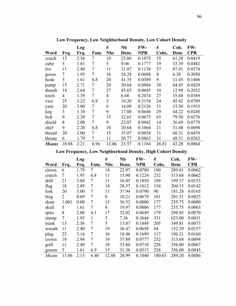
96
Low Frequency, Low Neighborhood Density, Low Cohort Density
Word
Frq.
Log Frq.
Fam.
# Nbs
Nb Dens.
FW-NPR
# Cohs.
Coh. Dens
FW-CPR
couch 13 2.56 7 10 23.86 0.1075 35 61.28 0.0419 cube 5 1.61 7 5 9.06 0.1777 19 33.39 0.0482 fox 11 2.40 7 11 21.07 0.1138 57 87.41 0.0274 goose 7 1.95 7 16 28.28 0.0688 8 6.38 0.3050 hook 5 1.61 6.8 20 41.35 0.0389 9 11.45 0.1406 pump 15 2.71 7 20 30.64 0.0884 38 64.45 0.0420 thumb 14 2.64 7 27 43.65 0.0605 10 12.99 0.2032 torch 4 1.39 7 4 6.68 0.2074 27 35.68 0.0389 vice 25 3.22 6.8 5 10.20 0.3154 24 45.42 0.0709 yarn 20 3.00 7 6 14.09 0.2126 11 15.50 0.1933 keg 3 1.10 7 9 17.00 0.0646 29 44.22 0.0248 bolt 9 2.20 7 15 32.65 0.0673 65 79.50 0.0276 shield 8 2.08 7 9 22.07 0.0942 14 26.69 0.0779 chef 9 2.20 6.8 10 20.64 0.1064 21 31.48 0.0698 thread 20 3.00 7 15 35.07 0.0854 31 68.31 0.0439 throne 6 1.79 7 11 20.77 0.0863 31 68.31 0.0262 Means 10.88 2.21 6.96 12.06 23.57 0.1184 26.81 43.28 0.0864
Low Frequency, Low Neighborhood Density, High Cohort Density
Word
Frq.
Log Frq.
Fam.
# Nbs
Nb Dens.
FW-NPR
# Cohs.
Coh. Dens
FW-CPR
clown 6 1.79 7 14 22.97 0.0780 190 289.81 0.0062 crutch 7 1.95 6.4 11 15.90 0.1224 232 313.68 0.0062 drill 21 3.04 7 11 16.45 0.1850 109 199.37 0.0153 flag 18 2.89 7 14 28.57 0.1012 154 204.15 0.0142 fork 20 3.00 7 11 37.94 0.0790 90 181.28 0.0165 frog 2 0.69 7 8 10.21 0.0679 161 281.51 0.0025 skate 1.001 0.00 7 15 36.52 0.0000 177 255.75 0.0000 skull 5 1.61 7 8 19.97 0.0806 177 255.75 0.0063 spire 8 2.08 4.1 17 32.02 0.0649 179 298.85 0.0070 stump 7 1.95 1 5 7.36 0.2644 331 623.00 0.0031 trunk 13 2.56 7 5 13.87 0.1849 205 349.81 0.0073 wreath 11 2.40 7 19 36.47 0.0658 84 152.29 0.0157 plug 23 3.14 7 16 18.46 0.1699 117 196.21 0.0160 crown 19 2.94 7 19 37.89 0.0777 232 313.68 0.0094 grill 11 2.40 7 18 33.80 0.0710 226 356.00 0.0067 groom 5 1.61 6.9 15 31.38 0.0513 226 356.00 0.0045 Means 11.06 2.13 6.40 12.88 24.99 0.1040 180.63 289.20 0.0086
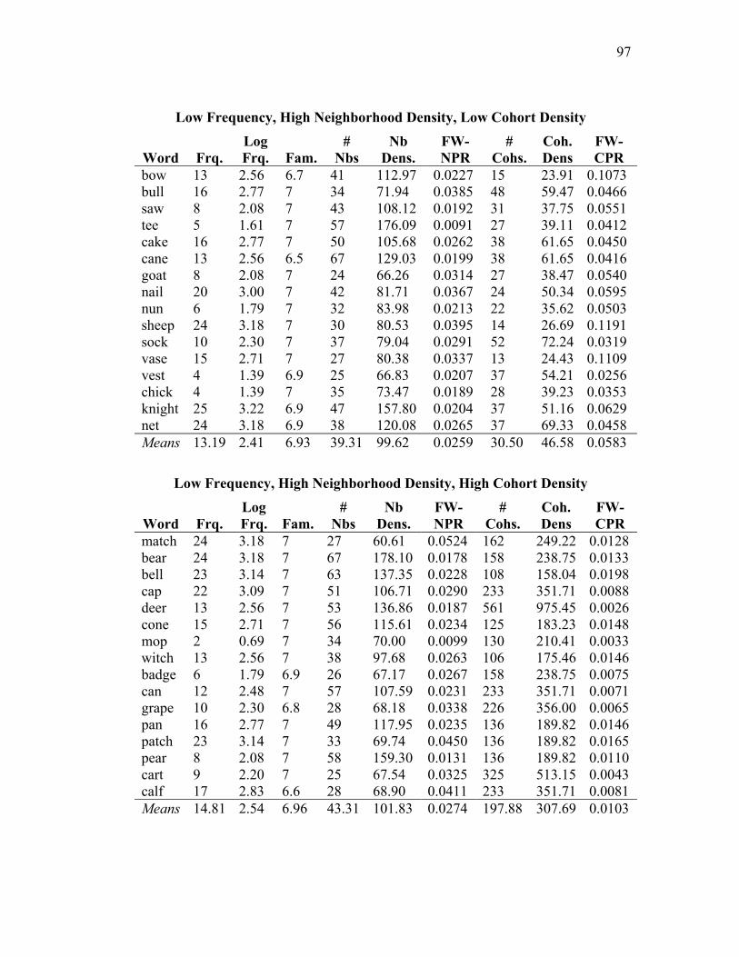
97
Low Frequency, High Neighborhood Density, Low Cohort Density
Word
Frq.
Log Frq.
Fam.
# Nbs
Nb Dens.
FW-NPR
# Cohs.
Coh. Dens
FW-CPR
bow 13 2.56 6.7 41 112.97 0.0227 15 23.91 0.1073 bull 16 2.77 7 34 71.94 0.0385 48 59.47 0.0466 saw 8 2.08 7 43 108.12 0.0192 31 37.75 0.0551 tee 5 1.61 7 57 176.09 0.0091 27 39.11 0.0412 cake 16 2.77 7 50 105.68 0.0262 38 61.65 0.0450 cane 13 2.56 6.5 67 129.03 0.0199 38 61.65 0.0416 goat 8 2.08 7 24 66.26 0.0314 27 38.47 0.0540 nail 20 3.00 7 42 81.71 0.0367 24 50.34 0.0595 nun 6 1.79 7 32 83.98 0.0213 22 35.62 0.0503 sheep 24 3.18 7 30 80.53 0.0395 14 26.69 0.1191 sock 10 2.30 7 37 79.04 0.0291 52 72.24 0.0319 vase 15 2.71 7 27 80.38 0.0337 13 24.43 0.1109 vest 4 1.39 6.9 25 66.83 0.0207 37 54.21 0.0256 chick 4 1.39 7 35 73.47 0.0189 28 39.23 0.0353 knight 25 3.22 6.9 47 157.80 0.0204 37 51.16 0.0629 net 24 3.18 6.9 38 120.08 0.0265 37 69.33 0.0458 Means 13.19 2.41 6.93 39.31 99.62 0.0259 30.50 46.58 0.0583
Low Frequency, High Neighborhood Density, High Cohort Density
Word
Frq.
Log Frq.
Fam.
# Nbs
Nb Dens.
FW-NPR
# Cohs.
Coh. Dens
FW-CPR
match 24 3.18 7 27 60.61 0.0524 162 249.22 0.0128 bear 24 3.18 7 67 178.10 0.0178 158 238.75 0.0133 bell 23 3.14 7 63 137.35 0.0228 108 158.04 0.0198 cap 22 3.09 7 51 106.71 0.0290 233 351.71 0.0088 deer 13 2.56 7 53 136.86 0.0187 561 975.45 0.0026 cone 15 2.71 7 56 115.61 0.0234 125 183.23 0.0148 mop 2 0.69 7 34 70.00 0.0099 130 210.41 0.0033 witch 13 2.56 7 38 97.68 0.0263 106 175.46 0.0146 badge 6 1.79 6.9 26 67.17 0.0267 158 238.75 0.0075 can 12 2.48 7 57 107.59 0.0231 233 351.71 0.0071 grape 10 2.30 6.8 28 68.18 0.0338 226 356.00 0.0065 pan 16 2.77 7 49 117.95 0.0235 136 189.82 0.0146 patch 23 3.14 7 33 69.74 0.0450 136 189.82 0.0165 pear 8 2.08 7 58 159.30 0.0131 136 189.82 0.0110 cart 9 2.20 7 25 67.54 0.0325 325 513.15 0.0043 calf 17 2.83 6.6 28 68.90 0.0411 233 351.71 0.0081 Means 14.81 2.54 6.96 43.31 101.83 0.0274 197.88 307.69 0.0103
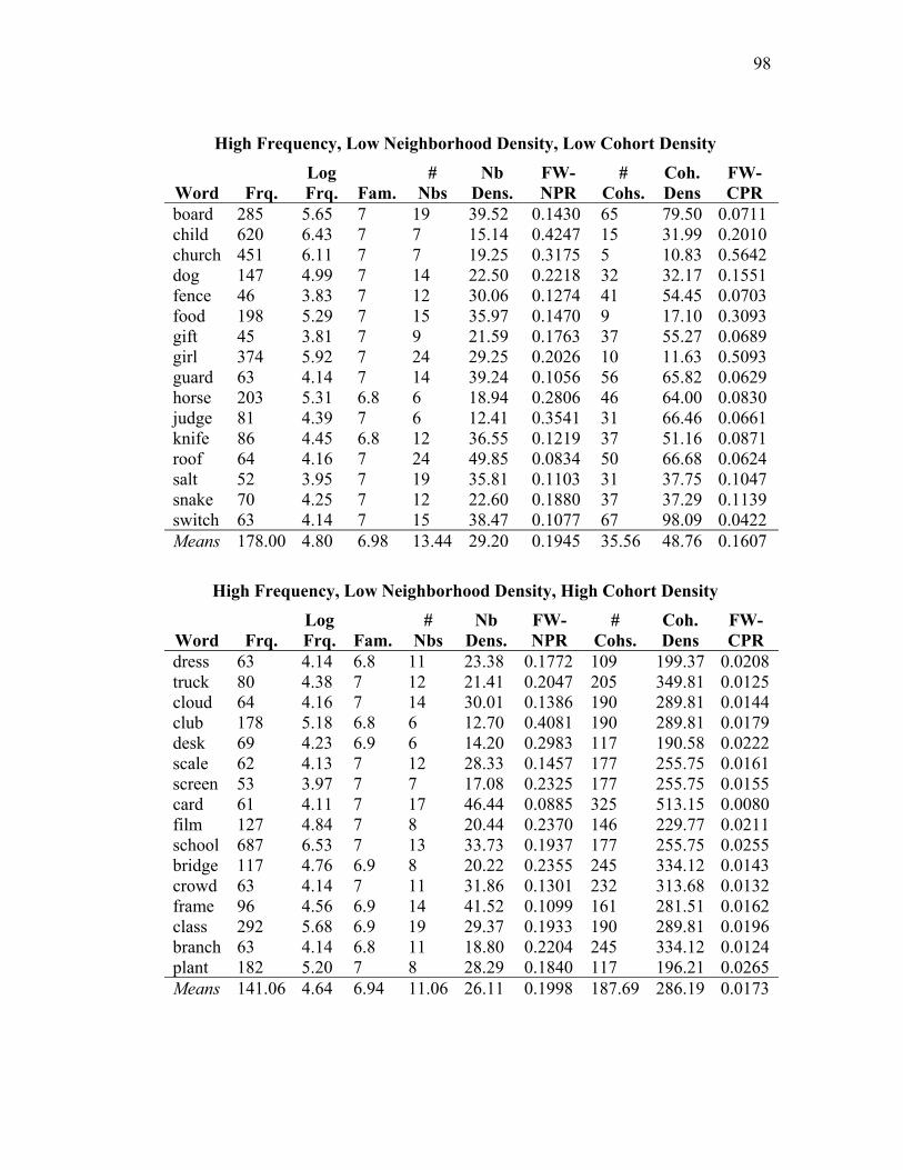
98
High Frequency, Low Neighborhood Density, Low Cohort Density
Word
Frq.
Log Frq.
Fam.
# Nbs
Nb Dens.
FW-NPR
# Cohs.
Coh. Dens
FW-CPR
board 285 5.65 7 19 39.52 0.1430 65 79.50 0.0711 child 620 6.43 7 7 15.14 0.4247 15 31.99 0.2010 church 451 6.11 7 7 19.25 0.3175 5 10.83 0.5642 dog 147 4.99 7 14 22.50 0.2218 32 32.17 0.1551 fence 46 3.83 7 12 30.06 0.1274 41 54.45 0.0703 food 198 5.29 7 15 35.97 0.1470 9 17.10 0.3093 gift 45 3.81 7 9 21.59 0.1763 37 55.27 0.0689 girl 374 5.92 7 24 29.25 0.2026 10 11.63 0.5093 guard 63 4.14 7 14 39.24 0.1056 56 65.82 0.0629 horse 203 5.31 6.8 6 18.94 0.2806 46 64.00 0.0830 judge 81 4.39 7 6 12.41 0.3541 31 66.46 0.0661 knife 86 4.45 6.8 12 36.55 0.1219 37 51.16 0.0871 roof 64 4.16 7 24 49.85 0.0834 50 66.68 0.0624 salt 52 3.95 7 19 35.81 0.1103 31 37.75 0.1047 snake 70 4.25 7 12 22.60 0.1880 37 37.29 0.1139 switch 63 4.14 7 15 38.47 0.1077 67 98.09 0.0422 Means 178.00 4.80 6.98 13.44 29.20 0.1945 35.56 48.76 0.1607
High Frequency, Low Neighborhood Density, High Cohort Density
Word
Frq.
Log Frq.
Fam.
# Nbs
Nb Dens.
FW-NPR
# Cohs.
Coh. Dens
FW-CPR
dress 63 4.14 6.8 11 23.38 0.1772 109 199.37 0.0208 truck 80 4.38 7 12 21.41 0.2047 205 349.81 0.0125 cloud 64 4.16 7 14 30.01 0.1386 190 289.81 0.0144 club 178 5.18 6.8 6 12.70 0.4081 190 289.81 0.0179 desk 69 4.23 6.9 6 14.20 0.2983 117 190.58 0.0222 scale 62 4.13 7 12 28.33 0.1457 177 255.75 0.0161 screen 53 3.97 7 7 17.08 0.2325 177 255.75 0.0155 card 61 4.11 7 17 46.44 0.0885 325 513.15 0.0080 film 127 4.84 7 8 20.44 0.2370 146 229.77 0.0211 school 687 6.53 7 13 33.73 0.1937 177 255.75 0.0255 bridge 117 4.76 6.9 8 20.22 0.2355 245 334.12 0.0143 crowd 63 4.14 7 11 31.86 0.1301 232 313.68 0.0132 frame 96 4.56 6.9 14 41.52 0.1099 161 281.51 0.0162 class 292 5.68 6.9 19 29.37 0.1933 190 289.81 0.0196 branch 63 4.14 6.8 11 18.80 0.2204 245 334.12 0.0124 plant 182 5.20 7 8 28.29 0.1840 117 196.21 0.0265 Means 141.06 4.64 6.94 11.06 26.11 0.1998 187.69 286.19 0.0173
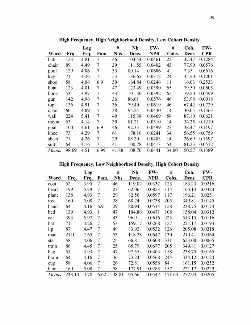
99
High Frequency, High Neighborhood Density, Low Cohort Density
Word
Frq.
Log Frq.
Fam.
# Nbs
Nb Dens.
FW-NPR
# Cohs.
Coh. Dens
FW-CPR
ball 123 4.81 7 46 104.44 0.0461 25 37.47 0.1284 chair 89 4.49 7 39 111.55 0.0402 43 77.90 0.0576 pool 129 4.86 7 35 80.14 0.0606 4 7.35 0.6616 key 71 4.26 7 53 136.65 0.0312 24 35.50 0.1201 shoe 58 4.06 6.9 50 164.84 0.0246 11 16.03 0.2533 boat 123 4.81 7 47 123.49 0.0390 65 79.50 0.0605 bone 53 3.97 7 43 101.30 0.0392 65 79.50 0.0499 gun 142 4.96 7 36 86.01 0.0576 46 53.98 0.0918 top 136 4.91 7 36 79.40 0.0619 46 67.42 0.0729 chain 60 4.09 7 38 95.24 0.0430 14 30.05 0.1363 wall 224 5.41 7 40 115.38 0.0469 58 87.19 0.0621 moon 63 4.14 7 30 81.21 0.0510 14 34.25 0.1210 goal 100 4.61 6.9 46 92.33 0.0499 27 38.47 0.1197 knee 73 4.29 7 61 178.16 0.0241 34 56.55 0.0759 sheet 71 4.26 7 29 88.20 0.0483 14 26.69 0.1597 suit 64 4.16 7 41 100.78 0.0413 54 81.23 0.0512 Means 98.69 4.51 6.99 41.88 108.70 0.0441 34.00 50.57 0.1389
High Frequency, Low Neighborhood Density, High Cohort Density
Word
Frq.
Log Frq.
Fam.
# Nbs
Nb Dens.
FW-NPR
# Cohs.
Coh. Dens
FW-CPR
coat 52 3.95 7 46 119.02 0.0332 125 183.23 0.0216heart 199 5.29 7 27 62.06 0.0853 115 163.14 0.0324plane 138 4.93 7 29 82.56 0.0597 117 196.21 0.0251tree 160 5.08 7 28 68.74 0.0738 205 349.81 0.0145band 64 4.16 6.9 29 80.94 0.0514 158 238.75 0.0174bed 139 4.93 1 47 104.86 0.0471 108 158.04 0.0312car 393 5.97 7 43 96.91 0.0616 325 513.15 0.0116hat 71 4.26 7 53 159.17 0.0268 157 221.17 0.0193lip 87 4.47 7 49 83.92 0.0532 126 205.08 0.0218man 2110 7.65 7 53 118.28 0.0647 130 210.41 0.0364star 58 4.06 7 25 66.81 0.0608 331 623.00 0.0065train 86 4.45 7 25 65.79 0.0677 205 349.81 0.0127bag 51 3.93 7 47 97.55 0.0403 158 238.75 0.0165brain 64 4.16 7 36 73.24 0.0568 245 334.12 0.0124cup 58 4.06 7 26 72.81 0.0558 84 161.15 0.0252hair 160 5.08 7 58 177.91 0.0285 157 221.17 0.0229Means 243.13 4.78 6.62 38.81 95.66 0.0542 171.63 272.94 0.0205


![SP2013F Lecture01 Introduction.ppt [相容模式]berlin.csie.ntnu.edu.tw/Courses/Speech Recognition... · 2013-09-11 · Spoken Dialogue: CMU’s Systems • Spoken language is attractive](https://img.pdfslide.net/doc/110x75/5f6cc674b6d30e3a690efdc4/sp2013f-lecture01-cberlincsientnuedutwcoursesspeech-recognition.jpg)