Embed Size (px)
Citation preview
The NCEP Climate Forecast System
S. SAHA, S. NADIGA, C. THIAW, J. WANG,Environmental Modeling Center, NOAA/NWS/NCEP/DOC, Washington, D.C.
W. WANG, Q. ZHANG, H. M. VAN DEN DOOL
Climate Prediction Center, NOAA/NWS/NCEP/DOC, Washington, D.C.
H.-L. PAN, S. MOORTHI, D. BEHRINGER, D. STOKES, M. PEÑA, S. LORD, G. WHITE
Environmental Modeling Center, NOAA/NWS/NCEP/DOC, Washington, D.C.
W. EBISUZAKI, P. PENG, AND P. XIE
Climate Prediction Center, NOAA/NWS/NCEP/DOC, Washington, D.C.
(Manuscript received 3 March 2005, in final form 8 August 2005)
ABSTRACT
The Climate Forecast System (CFS), the fully coupled ocean–land–atmosphere dynamical seasonal pre-diction system, which became operational at NCEP in August 2004, is described and evaluated in this paper.The CFS provides important advances in operational seasonal prediction on a number of fronts. For the firsttime in the history of U.S. operational seasonal prediction, a dynamical modeling system has demonstrateda level of skill in forecasting U.S. surface temperature and precipitation that is comparable to the skill of thestatistical methods used by the NCEP Climate Prediction Center (CPC). This represents a significantimprovement over the previous dynamical modeling system used at NCEP. Furthermore, the skill providedby the CFS spatially and temporally complements the skill provided by the statistical tools. The availabilityof a dynamical modeling tool with demonstrated skill should result in overall improvement in the opera-tional seasonal forecasts produced by CPC.
The atmospheric component of the CFS is a lower-resolution version of the Global Forecast System(GFS) that was the operational global weather prediction model at NCEP during 2003. The ocean com-ponent is the GFDL Modular Ocean Model version 3 (MOM3). There are several important improvementsinherent in the new CFS relative to the previous dynamical forecast system. These include (i) the atmo-sphere–ocean coupling spans almost all of the globe (as opposed to the tropical Pacific only); (ii) the CFSis a fully coupled modeling system with no flux correction (as opposed to the previous uncoupled “tier-2”system, which employed multiple bias and flux corrections); and (iii) a set of fully coupled retrospectiveforecasts covering a 24-yr period (1981–2004), with 15 forecasts per calendar month out to nine months intothe future, have been produced with the CFS.
These 24 years of fully coupled retrospective forecasts are of paramount importance to the propercalibration (bias correction) of subsequent operational seasonal forecasts. They provide a meaningful apriori estimate of model skill that is critical in determining the utility of the real-time dynamical forecast inthe operational framework. The retrospective dataset also provides a wealth of information for researchersto study interactive atmosphere–land–ocean processes.
1. IntroductionIt is generally assumed that the memory of the geo-
physical system that could aid in seasonal climate fore-casting resides mainly in the ocean. The strong El Niñoevents of 1982/83 and 1997/98 appeared to provide em-
pirical evidence that, at least in some cases, this is in-deed true (Barnston et al. 1999). It is thus logical for thescientific community to develop global coupled atmo-sphere–ocean models to aid in seasonal forecasting.
At the National Centers for Environmental Predic-tion (NCEP) in Washington, D.C., coupled ocean–atmosphere models are looked upon as an extension ofexisting numerical weather prediction infrastructure.For this task, one obviously needs numerical models ofboth the atmosphere and the ocean, along with their
Corresponding author address: Dr. Suranjana Saha, Environ-mental Modeling Center, 5200 Auth Road, Camp Springs, MD20746.E-mail: [email protected]
1 AUGUST 2006 S A H A E T A L . 3483
© 2006 American Meteorological Society
JCLI3812
own data assimilation systems. Global numerical pre-diction models for weather (and their attendant dataassimilation systems) have matured since about 1980and are the tool of choice today for day-to-day globalweather forecasting out to one or two weeks. On theother hand, while numerical prediction models for theocean coupled to an atmosphere have existed for a longtime in research mode (Manabe and Bryan 1969), suchmodels had not been tested in real-time forecasting, norhad a data assimilation system been developed for theocean until the 1990s.
Ji et al. (1995) described the early data assimilationeffort at NCEP [then the National Meteorological Cen-ter (NMC)] for a tropical strip of the Pacific Oceanusing the Modular Ocean Model version 1 (MOM1),developed at the Geophysical Fluid Dynamics Labora-tory (GFDL) in Princeton, New Jersey. An ocean re-analysis was performed by Ji et al. (1995) and Beh-ringer et al. (1998) for the Pacific basin (20°S–20°N)starting from July 1982 onward. This provided theocean initial conditions for coupled forecast experi-ments, including retrospective forecasts.
The first coupled forecast model at NCEP in the mid-1990s consisted of an ocean model for the PacificOcean, coupled to a coarser-resolution version of thethen operational NMC Medium Range Forecast(MRF) atmospheric model at a spectral triangular trun-cation of 40 waves (T40) in the horizontal and 18 sigmalevels (L18) in the vertical (Ji et al. 1994, 1998). Toavoid very large biases, “anomaly flux corrections”were applied at the ocean–atmosphere interface. Thefinal stand-alone atmospheric forecasts were made in“tier-2” mode in which the sea surface temperaturefields produced during the coupled integration wereused, after more bias correction, as a prescribed time-varying lower boundary condition for an ensemble ofatmospheric general circulation model (AGCM) runs.The tier-2 approach and its attendant flux correctionprocedure is common to this day. Since the SST outsidethe tropical Pacific had to be specified as well, dampedpersistence became a common substitute. This earlysetup of the coupled model was known as MRFb9x forthe atmospheric component and CMP12/14 for the oce-anic component. The atmospheric component was up-graded both in physics and resolution to T62L28 severalyears later (Kanamitsu et al. 2002b). This upgraded sys-tem, known as the Seasonal Forecast Model (SFM) wasoperational at NCEP until August 2004.
Very few operational centers have been able to af-ford the development of a high-resolution coupled at-mosphere–ocean–land model (no flux correction) forreal-time seasonal prediction. The European Centre forMedium-Range Weather Forecasts (ECMWF) has
been engaged in this effort along with NCEP. AtECMWF, the first coupled model (System-1) was de-veloped around 1996 (Stockdale et al. 1998), with asecond update (T95L40: System-2) in 2003 (Andersonet al. 2003). An evaluation against empirical models forall starting months during 1987–2001 can be found inVan Oldenborgh et al. (2003). In Australia, a coupledoperational system (at R21L9 resolution) was run inretrospective mode over the period 1981–95 from fourinitial months (Wang et al. 2002). In the United King-dom, similar operational efforts have been reported inGordon et al. (2000) and Pope et al. (2000). In Europe,a large research experiment was conducted recently,called the Development of a European Multimodel En-semble System for Seasonal to Interannual Prediction(DEMETER) in which seven different atmosphericmodels were coupled to about four ocean models; seePalmer et al. (2004). Other quasi-operational modelswith flux correction include the model described inKirtman (2003). At several other centers, such as theInternational Research Institute for Climate Prediction(IRI), the tier-2 system continues to be used (Barnstonet al. 2003). In research mode, there are many morecoupled models; see Schneider et al. (2003) for a recentoverview.
The purpose of this paper is to document the newNCEP Climate Forecast System (CFS), which becameoperational in August 2004. As part of the design of theCFS, three major improvements were made to the oldoperational coupled forecast system. First, the compo-nent models have been greatly modernized. The oceanmodel, MOM1, has been replaced by MOM3, and theatmospheric model, SFM, has been replaced by acoarse-resolution version of the operational (as of2003) NCEP Global Forecast System (GFS). Most no-tably, this change includes an upgrade in vertical reso-lution from the old SFM from 28 to 64 sigma layers.Second, the ocean–atmosphere coupling is now nearlyglobal (64°N–74°S), instead of only in the tropical Pa-cific Ocean, and flux correction is no longer applied.Thus, the CFS is a fully “tier-1” forecast system. Thecoupling over the global ocean required an importantupgrade in the ocean data assimilation as well (see D.Behringer et al. 2005, unpublished manuscript). Third,an extensive set of retrospective forecasts (“hindcasts”)was generated to cover a 24-yr period (1981–2004) inorder to obtain a history of the model. This history canbe used operationally to calibrate and assess the skill ofthe real-time forecasts. Hindcast histories that weregenerated to assess the skill of all previous tier-2 sea-sonal forecast systems in use at NCEP were obtained byprescribing “perfect” (observed) SST. This methodol-ogy is often assumed to provide an “upper limit of pre-
3484 J O U R N A L O F C L I M A T E VOLUME 19
dictability.” However, this method did not provide anaccurate estimate of the skill of the tier-2 operationalmodel, which used predicted, not perfect, SST. Thismethodology is still being practiced elsewhere to deter-mine the “skill” of multimodel ensembles, etc. In thecurrent CFS system, the model skill is assessed solely bythe use of a tier-1 retrospective set of forecasts.
The first two improvements include several advancesin physics and a much better coupled system, both inmultidecadal free runs (Wang et al. 2005) and in9-month forecasts from many initial conditions. Specifi-cally, the ENSO simulation and the synoptic tropicalactivity (the Madden–Julian oscillation, easterly waves,etc.) appear to be state of the art in the CFS with 64vertical levels. The third item, retrospective forecasts,while costly in terms of computer time and resources,are especially important since they provide a robustmeasure of skill to the user of these forecasts.
The layout of the paper is as follows: In sections 2and 3 we describe the components of the CFS and theorganization of the retrospective forecasts, respectively.In section 4 we discuss the CFS performance for itsmain application as a monthly/seasonal forecast tool. Insection 5 we present some diagnostics highlightingstrengths and systematic errors in the CFS. Summaryand conclusions are found in section 6.
2. Overview of the NCEP Climate ForecastSystem
The atmospheric component of the CFS is the NCEPatmospheric GFS model, as of February 2003 (Moorthiet al. 2001). Except for having a coarser horizontal reso-lution, it is the same as that used for operationalweather forecasting with no tuning for climate applica-tions. It adopts a spectral triangular truncation of 62waves (T62) in the horizontal (equivalent to nearly a200-km Gaussian grid) and a finite differencing in thevertical with 64 sigma layers. The model top is at 0.2hPa. This version of the GFS has been modified fromthe version of the NCEP model used for the NCEP–National Center for Atmospheric Research (NCAR)reanalysis (Kalnay et al. 1996; Kistler et al. 2001), withupgrades in the parameterization of solar radiationtransfer (Hou et al. 1996, 2002), boundary layer verticaldiffusion (Hong and Pan 1996), cumulus convection(Hong and Pan 1998), and gravity wave drag (Kim andArakawa 1995). In addition, the cloud condensate is aprognostic quantity with a simple cloud microphysicsparameterization (Zhao and Carr 1997; Sundqvist et al.1989; Moorthi et al. 2001). The fractional cloud coverused for radiation is diagnostically determined by thepredicted cloud condensate.
The oceanic component is the GFDL ModularOcean Model version 3 (MOM3) (Pacanowski andGriffies 1998), which is a finite difference version of theocean primitive equations under the assumptions ofBoussinesq and hydrostatic approximations. It usesspherical coordinates in the horizontal with a staggeredArakawa B grid and the z coordinate in the vertical.The ocean surface boundary is computed as an explicitfree surface. The domain is quasi-global extending from74°S to 64°N. The zonal resolution is 1°. The meridionalresolution is 1⁄3° between 10°S and 10°N, gradually in-creasing through the Tropics until becoming fixed at 1°poleward of 30°S and 30°N. There are 40 layers in thevertical with 27 layers in the upper 400 m, and thebottom depth is around 4.5 km. The vertical resolutionis 10 m from the surface to the 240-m depth, graduallyincreasing to about 511 m in the bottom layer. Verticalmixing follows the nonlocal K-profile parameterizationof Large et al. (1994). The horizontal mixing of tracersuses the isoneutral method pioneered by Gent andMcWilliams (1990; see also Griffies et al. 1998). Thehorizontal mixing of momentum uses the nonlinearscheme of Smagorinsky (1963).
The atmospheric and oceanic components arecoupled with no flux adjustment or correction. The twocomponents exchange daily averaged quantities, suchas heat and momentum fluxes, once a day. Because ofthe difference in latitudinal domain, full interaction be-tween atmospheric and oceanic components is confinedto 65°S to 50°N. Poleward of 74°S and 64°N, SSTsneeded for the atmospheric model are taken from ob-served climatology. Between 74° and 65°S and between64° and 50°N, SSTs for the atmospheric component area weighted average of the observed climatology and theSST from the ocean component of the CFS. Theweights vary linearly with latitude such that the SSTs at74°S and 64°N equal observed climatology and theSSTs from 65°S and 50°N equal values from the oceancomponent. Sea ice extent is prescribed from the ob-served climatology.
The ocean initial conditions were obtained from theGlobal Ocean Data Assimilation System (GODAS; D.Behringer et al. 2005, unpublished manuscript), whichwas made operational at NCEP in September 2003. Theocean model used in GODAS is the same as that usedin the CFS retrospective forecasts. The ocean data as-similation system uses the 3D variational technique ofDerber and Rosati (1989), modified to include verticalvariations in the error covariances (Behringer et al.1998). The ocean model in GODAS was forced withweekly fluxes of heat (Q), surface buoyancy fluxes (E �P) and wind stress vectors (�) from NCEP Reanalysis-2(R2: Kanamitsu et al. 2002a). The GODAS sea surface
1 AUGUST 2006 S A H A E T A L . 3485
temperatures were relaxed to Reynolds SST (Reynoldset al. 2002) with a time scale of 5 days. Similarly, the seasurface salinity (SSS) was relaxed to Levitus monthlyclimatological SSS fields (Levitus et al. 1994) but with atime scale of 10 days. The subsurface temperature datathat were assimilated were obtained from expendablebathythermographs (XBTs), the tropical atmosphere–ocean (TAO) array of moored buoys, and Argo andArgo-like floats. The subsurface salinity variabilitystrongly influences the density stratification in theocean through the formation of salt-stratified barrierlayers, especially in the western and central equatorialPacific Ocean (Maes and Behringer 2000; Ji et al. 2000).Therefore, synthetic salinity data were created by im-posing a climatological temperature–salinity (T–S) re-lationship on the observed subsurface temperature pro-files, and these synthetic salinity profiles were assimi-lated during the ocean model runs.
For the prediction of land surface hydrology, a two-layer model described in Mahrt and Pan (1984) is usedin the CFS.
3. Design of the CFS retrospective forecasts
The CFS includes a comprehensive set of retrospec-tive runs that are used to calibrate and evaluate the skillof its forecasts. Each run is a full 9-month integration.The retrospective period covers all 12 calendar monthsin the 24 years from 1981 to 2004. Runs are initiatedfrom 15 initial conditions that span each month,amounting to a total of 4320 runs. Since each run is a9-month integration, the CFS was run for an equivalentof 3240 yr! Owing to limitations in computer time, only15 days in the month were used as initial conditions.These initial conditions were carefully selected to spanthe evolution of both the atmosphere and ocean in acontinuous fashion.
The atmospheric initial conditions were from theNCEP/Department of Energy Atmospheric Model In-tercomparison Project (AMIP) R2 data (Kanamitsu etal. 2002a), and the ocean initial conditions were fromthe NCEP Global Ocean Data Assimilation (GODAS)(D. Behringer et al. 2005, unpublished manuscript).Each month was partitioned into three segments. Thefirst was centered on the pentad ocean initial conditionas the 11th of the month, that is, the five atmosphericinitial states of the 9th, 10th, 11th, 12th, and 13th of themonth used the same pentad ocean initial condition asthe 11th. The second set of five atmospheric initialstates of the 19th, 20th, 21st, 22d, and 23d of the monthused the same pentad ocean initial condition as the 21stof the month. The last set of five atmospheric initialstates include the second-to-last day of the month, the
last day of the month, and the first, second, and thirddays of the next month. This last set uses the samepentad ocean initial condition of the first of the nextmonth. These 15 runs from the retrospective forecastsform the ensemble that is used by operational forecast-ers for calibration and skill assessment for the opera-tional monthly seasonal forecast at NCEP. Note that noperturbations of the initial conditions are applied formaking the ensemble forecast. The perturbations comeautomatically by taking atmospheric states one dayapart, but this may not be optimal.
A hypothetical example is the official monthly/sea-sonal forecast made by the Climate Prediction Center(CPC) of NCEP on the third Thursday of February.February is then considered to be the month of forecastlead zero (not issued), March is the month of forecastlead one (or lead 0.5 more precisely), and so on. Runsoriginating from initial conditions after 3 Februaryfrom the retrospective forecasts are not considered forcalibration of the March, April, etc. forecasts. This isdone because in “operations” there is a 7-day lag inobtaining the ocean initial conditions (see appendix Bfor more on the design of operational CFS forecasts).The 15 members in the ensemble thus include 9–13January, 19–23 January, and 30 January–3 of February.This method of calibration and subsequent skill assess-ment is used throughout this paper in order to replicatethe operational procedures used at NCEP and to pro-vide the most accurate assessment possible of the CFSskill to the forecasting community.
It is important to note that the CFS model codeswere “frozen” in June 2003. The running of the entireretrospective forecasts and operational implementationof the CFS that took nearly a year were made withthese codes. No changes or tuning for results weremade to these codes during the execution of the fore-casts. These forecasts truly represent the “history” ofthe operational CFS.
4. CFS performance statistics
In this section we review the performance of CFSretrospective forecasts, first in terms of skill as mea-sured by the anomaly correlation (AC) against obser-vations (section 4a), and then in terms of probabilityforecasts (section 4b). The “observations” used for theverification of the CFS forecasts require further expla-nation. Ideally, if the model analysis is good enough tobe used as the initial condition, it should also be usablefor verification, as is frequently done in weather fore-casting. Over the years, NWP forecasts and analyseshave improved hand-in-hand. However, we may not yethave reached that level of sophistication with coupledmodels.
3486 J O U R N A L O F C L I M A T E VOLUME 19
(i) All SST forecasts here are verified against opti-mum interpolation SST (OISST) version 2 (Reyn-olds et al. 2002), which is the water temperature atthe surface, while GODAS “SST” is the watertemperature at 5 m below the surface. While in thetropical Pacific, SST forecast verifications againsteither GODAS or OIv2 are very close; the differ-ences in verification scores are large in midlati-tudes.
(ii) For surface weather elements over the continentalUnited States, we use the so-called Climate Divi-sion data (Gutman and Quayle 1996), a highlyquality controlled dataset maintained at the U.S.National Climatic Data Center (NCDC). For tem-perature over land outside the United States weuse the R2 fields (Kanamitsu et al. 2002a), whilefor precipitation we use the CPC Merged Analysisof Precipitation (CMAP) Xie–Arkin dataset (Xieand Arkin 1997). The R2 temperature field maynot be very good, but it is unlikely that the skill ofthe forecast is overestimated.
(iii) Verification of 500-hPa geopotential and somemajor atmospheric indices, such as the North At-lantic Oscillation (NAO) and the Pacific–NorthAmerican (PNA) pattern, is done against R2fields.
(iv) The most dubious case of verification is for soilmoisture. Here we use the R2 fields and justify thisas follows: 1) The R2 is forced by observed pre-cipitation, albeit with a delay of one pentad, andshould be more realistic than soil moisture pro-duced by traditional data assimilation systems, likethe first reanalysis (Kalnay et al. 1996); and 2) theR2 is consistent in model formulation with the CFSforecasts. If an independent product, such as thenonoperational global leaky bucket calculations(Fan and van den Dool 2004), were to be used forverification, one first needs to transpose one prod-uct into the other, an activity fraught with diffi-culty.
a. Verification of the ensemble mean
We refer to appendix A for details about definitions,and the adjustments necessary in using the anomalycorrelation (AC) in the context of (i) systematic errorcorrection and (ii) cross validation (CV), which hasbeen adhered to in computing the results presented inthis paper. In this section we correct for the overallmean error by subtracting the model climatology frommodel forecasts. See details in appendix A.
We focus on, in order, the prediction of SST in theNiño-3.4 area (5°S–5°N, 170°–120°W) of the tropicalPacific, SST in midlatitudes, surface air temperature,
precipitation, 500-hPa geopotential, and soil moisture.In all cases we verify either monthly or seasonal meanvalues. In most cases, we verify the bias-corrected en-semble mean averaged over the 15 ensemble members.In some cases, we also compare to other methods: ei-ther a previous model or some of the statistical toolsthat are being used by CPC. When we quote scores for1981–2003, this includes verifying data well into 2004for the longer lead forecasts starting in 2003.
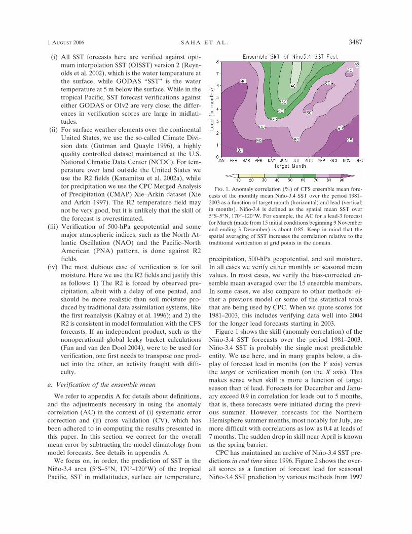
Figure 1 shows the skill (anomaly correlation) of theNiño-3.4 SST forecasts over the period 1981–2003.Niño-3.4 SST is probably the single most predictableentity. We use here, and in many graphs below, a dis-play of forecast lead in months (on the Y axis) versusthe target or verification month (on the X axis). Thismakes sense when skill is more a function of targetseason than of lead. Forecasts for December and Janu-ary exceed 0.9 in correlation for leads out to 5 months,that is, these forecasts were initiated during the previ-ous summer. However, forecasts for the NorthernHemisphere summer months, most notably for July, aremore difficult with correlations as low as 0.4 at leads of7 months. The sudden drop in skill near April is knownas the spring barrier.
CPC has maintained an archive of Niño-3.4 SST pre-dictions in real time since 1996. Figure 2 shows the over-all scores as a function of forecast lead for seasonalNiño-3.4 SST prediction by various methods from 1997
FIG. 1. Anomaly correlation (%) of CFS ensemble mean fore-casts of the monthly mean Niño-3.4 SST over the period 1981–2003 as a function of target month (horizontal) and lead (vertical;in months). Niño-3.4 is defined as the spatial mean SST over5°S–5°N, 170°–120°W. For example, the AC for a lead-3 forecastfor March (made from 15 initial conditions beginning 9 Novemberand ending 3 December) is about 0.85. Keep in mind that thespatial averaging of SST increases the correlation relative to thetraditional verification at grid points in the domain.
1 AUGUST 2006 S A H A E T A L . 3487
Fig 1 live 4/C
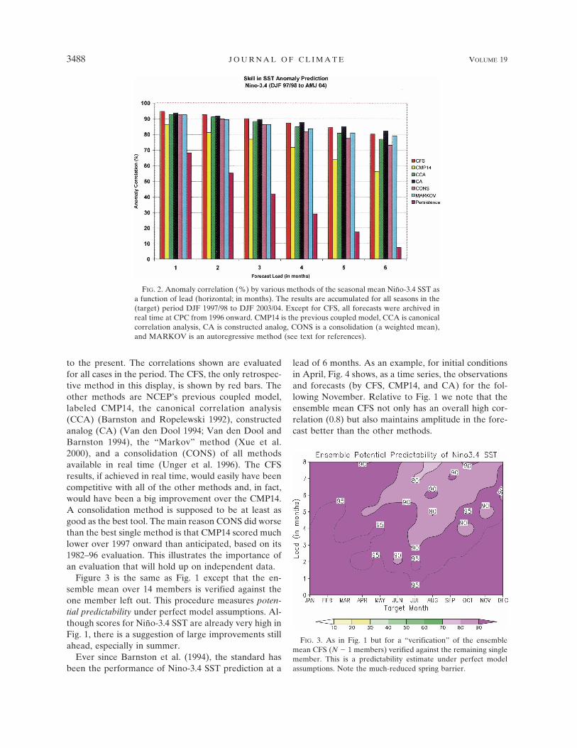
to the present. The correlations shown are evaluatedfor all cases in the period. The CFS, the only retrospec-tive method in this display, is shown by red bars. Theother methods are NCEP’s previous coupled model,labeled CMP14, the canonical correlation analysis(CCA) (Barnston and Ropelewski 1992), constructedanalog (CA) (Van den Dool 1994; Van den Dool andBarnston 1994), the “Markov” method (Xue et al.2000), and a consolidation (CONS) of all methodsavailable in real time (Unger et al. 1996). The CFSresults, if achieved in real time, would easily have beencompetitive with all of the other methods and, in fact,would have been a big improvement over the CMP14.A consolidation method is supposed to be at least asgood as the best tool. The main reason CONS did worsethan the best single method is that CMP14 scored muchlower over 1997 onward than anticipated, based on its1982–96 evaluation. This illustrates the importance ofan evaluation that will hold up on independent data.
Figure 3 is the same as Fig. 1 except that the en-semble mean over 14 members is verified against theone member left out. This procedure measures poten-tial predictability under perfect model assumptions. Al-though scores for Niño-3.4 SST are already very high inFig. 1, there is a suggestion of large improvements stillahead, especially in summer.
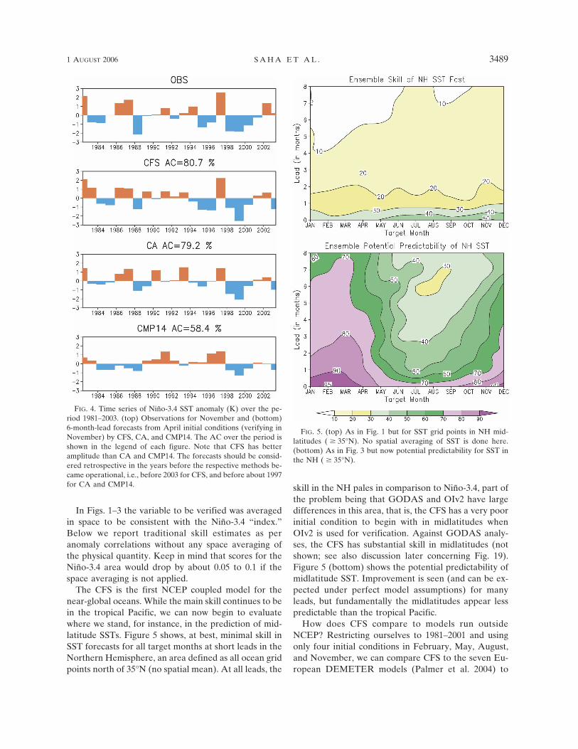
Ever since Barnston et al. (1994), the standard hasbeen the performance of Nino-3.4 SST prediction at a
lead of 6 months. As an example, for initial conditionsin April, Fig. 4 shows, as a time series, the observationsand forecasts (by CFS, CMP14, and CA) for the fol-lowing November. Relative to Fig. 1 we note that theensemble mean CFS not only has an overall high cor-relation (0.8) but also maintains amplitude in the fore-cast better than the other methods.
FIG. 3. As in Fig. 1 but for a “verification” of the ensemblemean CFS (N � 1 members) verified against the remaining singlemember. This is a predictability estimate under perfect modelassumptions. Note the much-reduced spring barrier.
FIG. 2. Anomaly correlation (%) by various methods of the seasonal mean Niño-3.4 SST asa function of lead (horizontal; in months). The results are accumulated for all seasons in the(target) period DJF 1997/98 to DJF 2003/04. Except for CFS, all forecasts were archived inreal time at CPC from 1996 onward. CMP14 is the previous coupled model, CCA is canonicalcorrelation analysis, CA is constructed analog, CONS is a consolidation (a weighted mean),and MARKOV is an autoregressive method (see text for references).
3488 J O U R N A L O F C L I M A T E VOLUME 19
Fig 2 live 4/C Fig 3 live 4/C
In Figs. 1–3 the variable to be verified was averagedin space to be consistent with the Niño-3.4 “index.”Below we report traditional skill estimates as peranomaly correlations without any space averaging ofthe physical quantity. Keep in mind that scores for theNiño-3.4 area would drop by about 0.05 to 0.1 if thespace averaging is not applied.
The CFS is the first NCEP coupled model for thenear-global oceans. While the main skill continues to bein the tropical Pacific, we can now begin to evaluatewhere we stand, for instance, in the prediction of mid-latitude SSTs. Figure 5 shows, at best, minimal skill inSST forecasts for all target months at short leads in theNorthern Hemisphere, an area defined as all ocean gridpoints north of 35°N (no spatial mean). At all leads, the
skill in the NH pales in comparison to Niño-3.4, part ofthe problem being that GODAS and OIv2 have largedifferences in this area, that is, the CFS has a very poorinitial condition to begin with in midlatitudes whenOIv2 is used for verification. Against GODAS analy-ses, the CFS has substantial skill in midlatitudes (notshown; see also discussion later concerning Fig. 19).Figure 5 (bottom) shows the potential predictability ofmidlatitude SST. Improvement is seen (and can be ex-pected under perfect model assumptions) for manyleads, but fundamentally the midlatitudes appear lesspredictable than the tropical Pacific.
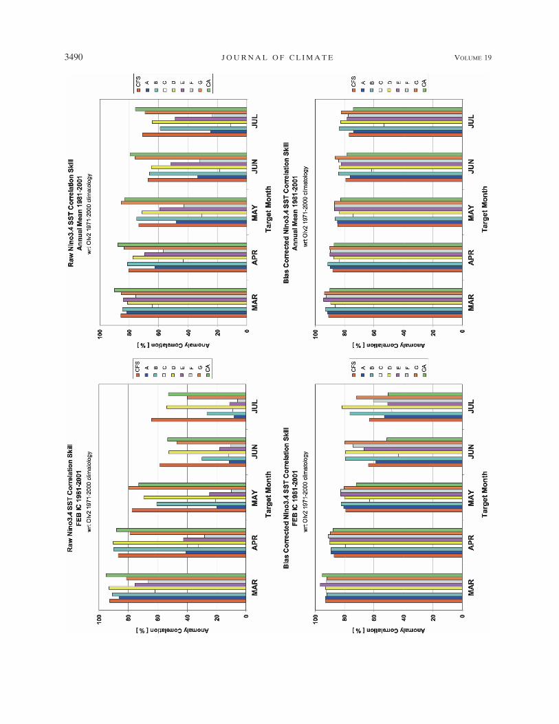
How does CFS compare to models run outsideNCEP? Restricting ourselves to 1981–2001 and usingonly four initial conditions in February, May, August,and November, we can compare CFS to the seven Eu-ropean DEMETER models (Palmer et al. 2004) to
FIG. 4. Time series of Niño-3.4 SST anomaly (K) over the pe-riod 1981–2003. (top) Observations for November and (bottom)6-month-lead forecasts from April initial conditions (verifying inNovember) by CFS, CA, and CMP14. The AC over the period isshown in the legend of each figure. Note that CFS has betteramplitude than CA and CMP14. The forecasts should be consid-ered retrospective in the years before the respective methods be-came operational, i.e., before 2003 for CFS, and before about 1997for CA and CMP14.
FIG. 5. (top) As in Fig. 1 but for SST grid points in NH mid-latitudes ( � 35°N). No spatial averaging of SST is done here.(bottom) As in Fig. 3 but now potential predictability for SST inthe NH ( � 35°N).
1 AUGUST 2006 S A H A E T A L . 3489
Fig 4 live 4/C Fig 5 live 4/C
3490 J O U R N A L O F C L I M A T E VOLUME 19
Fig 6 live 4/C
which we further add CPC’s constructed analog (Vanden Dool 1994). Figure 6 (left) shows the anomaly cor-relation for the nine models in forecasting Niño-3.4 SSTfrom initial conditions in early February at lead 1 (forMarch) out to lead 5 (July). We have shown the CFSand CA, but marked the European models as A–G.The anomalies are relative to observed 1971–2000 cli-matology. The upper (left) display is for raw forecasts,while the lower (left) display is for systematic error-corrected forecasts (using cross-validation and leaving3 years out). Forecasts from February initial conditions,just before the spring barrier, are the hardest to predict,and without bias correction some methods have a realproblem. Perhaps surprisingly, the systematic error cor-rection improves the score of many of the poor per-formers, indicating a linearly working system. For in-stance, model A improves its score from 0.2 to 0.8 cor-relation at lead 3. The CFS and CA have very littlesystematic error and do not profit from this correction.The right-hand panels in Figure 6 show the results of allfour initial conditions combined. The later starts (May,August, and October) have much higher anomaly cor-relation scores than February initial conditions, so theannual mean scores look good and are much betterthan February. Annual mean scores for persistence areconsiderably lower than for any of the methods (aftersystematic error correction), but for initial conditions inNovember persistence is also very high.
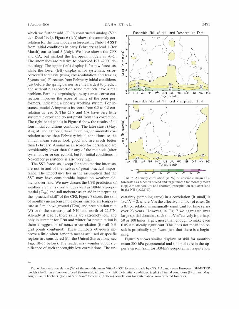
The SST forecasts, except for some marine interests,are not in and of themselves of great practical impor-tance. The importance lies in the assumption that theSST may have considerable impact on weather ele-ments over land. We now discuss the CFS prediction ofweather elements over land, as well as 500-hPa geopo-tential (Z500) and soil moisture as an aid in interpretingthe “practical skill” of the CFS. Figure 7 shows the skillof monthly mean (ensemble mean) surface air tempera-ture at 2 m above ground (T2m) and precipitation rate(P) over the extratropical NH land north of 22.5°N.Already at lead 1, these skills are extremely low, andonly in summer for T2m and winter for precipitation isthere a suggestion of nonzero correlation (for all NHgrid points combined). These numbers obviously im-prove a little when 3-month means are used or specificregions are considered (for the United States alone, seeFigs. 10–15 below). The reader may wonder about sig-nificance of such thoroughly low correlations. The un-
certainty (sampling error) in a correlation (if small) is1/� N � 2, where N is the effective number of cases. Soa 0.4 correlation is marginally significant for time seriesover 23 years. However, in Fig. 7 we aggregate overlarge spatial domains, such that N effectively is perhaps50 or 100 times larger, more than enough to make even0.05 statistically significant. This does not mean the re-sult is practically significant, just that there is a begin-ning.
Figure 8 shows similar displays of skill for monthlymean 500-hPa geopotential and soil moisture in the up-per 2-m soil. Skill for 500-hPa geopotential is quite low
←
FIG. 6. Anomaly correlation (%) of the monthly mean Niño-3.4 SST forecasts made by CFS, CA, and seven European DEMETERmodels (A–G), as a function of lead (horizontal; in months). (left) Feb initial conditions; (right) all initial conditions (February, May,August, and October). (top) ACs of “raw” forecasts; (bottom) correlations for systematic-error-corrected forecasts.
FIG. 7. Anomaly correlation (in %) of ensemble mean CFSforecasts as a function of lead and target month for monthly mean(top) 2-m temperature and (bottom) precipitation rate over landin the NH (�22.5°N).
1 AUGUST 2006 S A H A E T A L . 3491
Fig 7 live 4/C
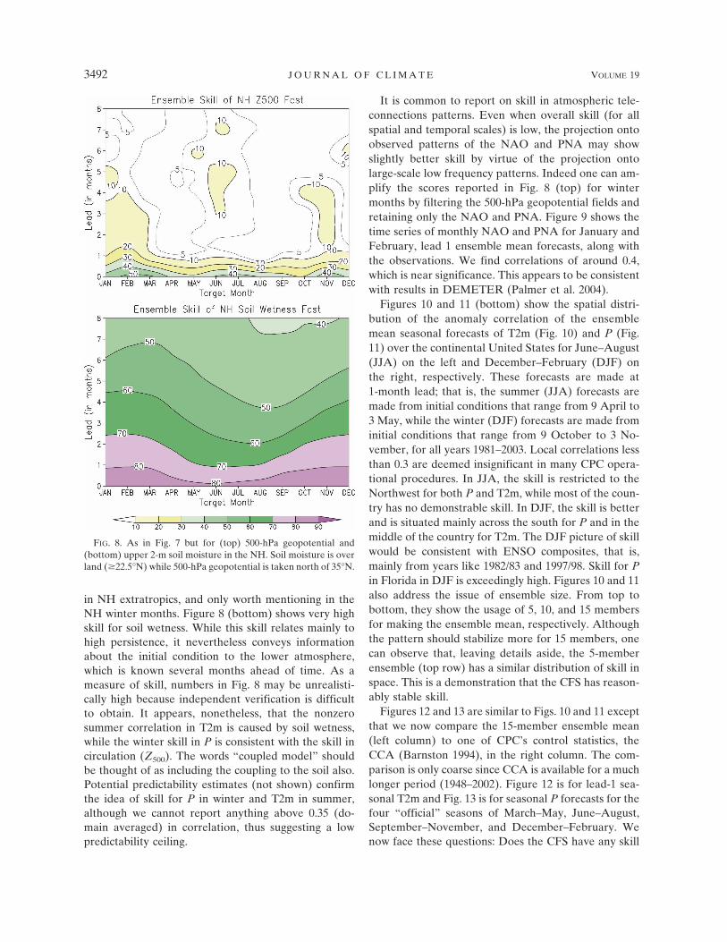
in NH extratropics, and only worth mentioning in theNH winter months. Figure 8 (bottom) shows very highskill for soil wetness. While this skill relates mainly tohigh persistence, it nevertheless conveys informationabout the initial condition to the lower atmosphere,which is known several months ahead of time. As ameasure of skill, numbers in Fig. 8 may be unrealisti-cally high because independent verification is difficultto obtain. It appears, nonetheless, that the nonzerosummer correlation in T2m is caused by soil wetness,while the winter skill in P is consistent with the skill incirculation (Z500). The words “coupled model” shouldbe thought of as including the coupling to the soil also.Potential predictability estimates (not shown) confirmthe idea of skill for P in winter and T2m in summer,although we cannot report anything above 0.35 (do-main averaged) in correlation, thus suggesting a lowpredictability ceiling.
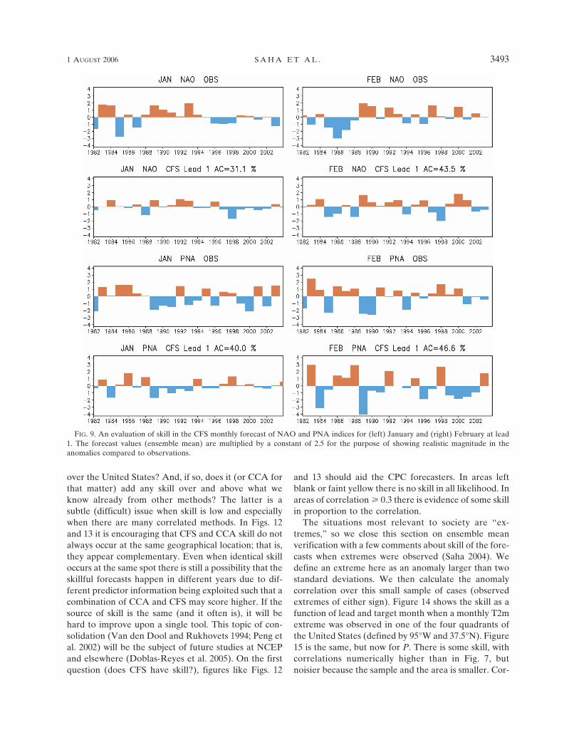
It is common to report on skill in atmospheric tele-connections patterns. Even when overall skill (for allspatial and temporal scales) is low, the projection ontoobserved patterns of the NAO and PNA may showslightly better skill by virtue of the projection ontolarge-scale low frequency patterns. Indeed one can am-plify the scores reported in Fig. 8 (top) for wintermonths by filtering the 500-hPa geopotential fields andretaining only the NAO and PNA. Figure 9 shows thetime series of monthly NAO and PNA for January andFebruary, lead 1 ensemble mean forecasts, along withthe observations. We find correlations of around 0.4,which is near significance. This appears to be consistentwith results in DEMETER (Palmer et al. 2004).
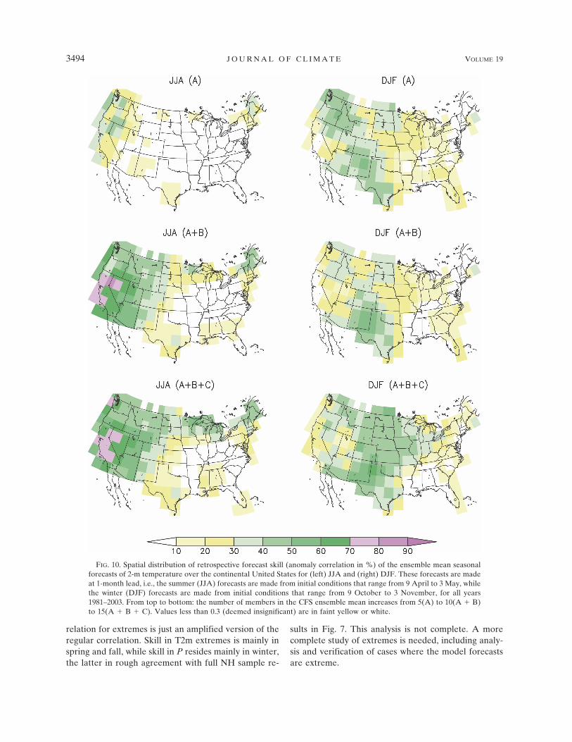
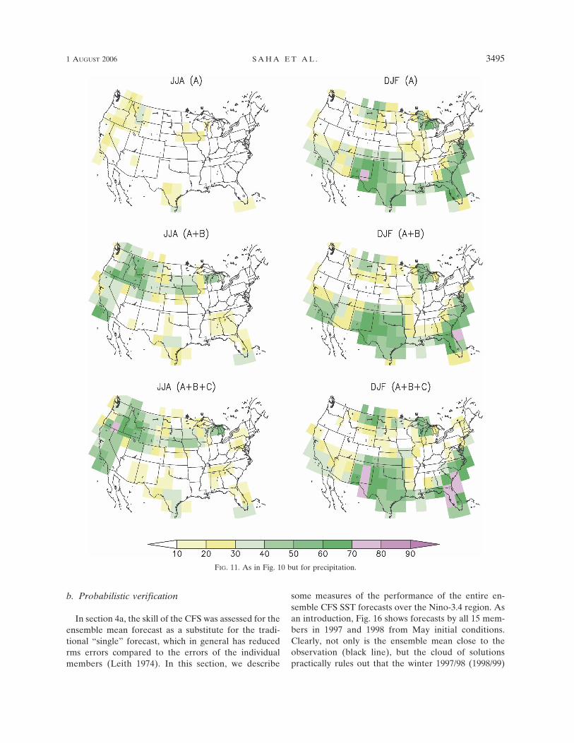
Figures 10 and 11 (bottom) show the spatial distri-bution of the anomaly correlation of the ensemblemean seasonal forecasts of T2m (Fig. 10) and P (Fig.11) over the continental United States for June–August(JJA) on the left and December–February (DJF) onthe right, respectively. These forecasts are made at1-month lead; that is, the summer (JJA) forecasts aremade from initial conditions that range from 9 April to3 May, while the winter (DJF) forecasts are made frominitial conditions that range from 9 October to 3 No-vember, for all years 1981–2003. Local correlations lessthan 0.3 are deemed insignificant in many CPC opera-tional procedures. In JJA, the skill is restricted to theNorthwest for both P and T2m, while most of the coun-try has no demonstrable skill. In DJF, the skill is betterand is situated mainly across the south for P and in themiddle of the country for T2m. The DJF picture of skillwould be consistent with ENSO composites, that is,mainly from years like 1982/83 and 1997/98. Skill for Pin Florida in DJF is exceedingly high. Figures 10 and 11also address the issue of ensemble size. From top tobottom, they show the usage of 5, 10, and 15 membersfor making the ensemble mean, respectively. Althoughthe pattern should stabilize more for 15 members, onecan observe that, leaving details aside, the 5-memberensemble (top row) has a similar distribution of skill inspace. This is a demonstration that the CFS has reason-ably stable skill.
Figures 12 and 13 are similar to Figs. 10 and 11 exceptthat we now compare the 15-member ensemble mean(left column) to one of CPC’s control statistics, theCCA (Barnston 1994), in the right column. The com-parison is only coarse since CCA is available for a muchlonger period (1948–2002). Figure 12 is for lead-1 sea-sonal T2m and Fig. 13 is for seasonal P forecasts for thefour “official” seasons of March–May, June–August,September–November, and December–February. Wenow face these questions: Does the CFS have any skill
FIG. 8. As in Fig. 7 but for (top) 500-hPa geopotential and(bottom) upper 2-m soil moisture in the NH. Soil moisture is overland (�22.5°N) while 500-hPa geopotential is taken north of 35°N.
3492 J O U R N A L O F C L I M A T E VOLUME 19
Fig 8 live 4/C
over the United States? And, if so, does it (or CCA forthat matter) add any skill over and above what weknow already from other methods? The latter is asubtle (difficult) issue when skill is low and especiallywhen there are many correlated methods. In Figs. 12and 13 it is encouraging that CFS and CCA skill do notalways occur at the same geographical location; that is,they appear complementary. Even when identical skilloccurs at the same spot there is still a possibility that theskillful forecasts happen in different years due to dif-ferent predictor information being exploited such that acombination of CCA and CFS may score higher. If thesource of skill is the same (and it often is), it will behard to improve upon a single tool. This topic of con-solidation (Van den Dool and Rukhovets 1994; Peng etal. 2002) will be the subject of future studies at NCEPand elsewhere (Doblas-Reyes et al. 2005). On the firstquestion (does CFS have skill?), figures like Figs. 12
and 13 should aid the CPC forecasters. In areas leftblank or faint yellow there is no skill in all likelihood. Inareas of correlation � 0.3 there is evidence of some skillin proportion to the correlation.
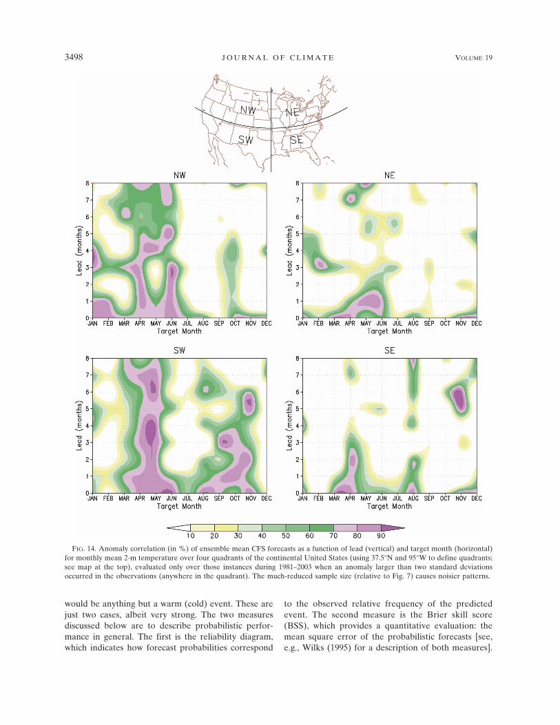
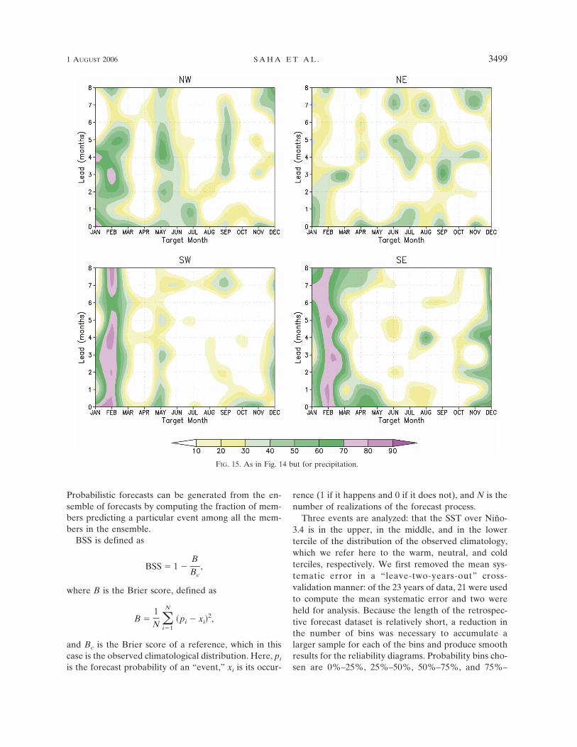
The situations most relevant to society are “ex-tremes,” so we close this section on ensemble meanverification with a few comments about skill of the fore-casts when extremes were observed (Saha 2004). Wedefine an extreme here as an anomaly larger than twostandard deviations. We then calculate the anomalycorrelation over this small sample of cases (observedextremes of either sign). Figure 14 shows the skill as afunction of lead and target month when a monthly T2mextreme was observed in one of the four quadrants ofthe United States (defined by 95°W and 37.5°N). Figure15 is the same, but now for P. There is some skill, withcorrelations numerically higher than in Fig. 7, butnoisier because the sample and the area is smaller. Cor-
FIG. 9. An evaluation of skill in the CFS monthly forecast of NAO and PNA indices for (left) January and (right) February at lead1. The forecast values (ensemble mean) are multiplied by a constant of 2.5 for the purpose of showing realistic magnitude in theanomalies compared to observations.
1 AUGUST 2006 S A H A E T A L . 3493
Fig 9 live 4/C
relation for extremes is just an amplified version of theregular correlation. Skill in T2m extremes is mainly inspring and fall, while skill in P resides mainly in winter,the latter in rough agreement with full NH sample re-
sults in Fig. 7. This analysis is not complete. A morecomplete study of extremes is needed, including analy-sis and verification of cases where the model forecastsare extreme.
FIG. 10. Spatial distribution of retrospective forecast skill (anomaly correlation in %) of the ensemble mean seasonalforecasts of 2-m temperature over the continental United States for (left) JJA and (right) DJF. These forecasts are madeat 1-month lead, i.e., the summer (JJA) forecasts are made from initial conditions that range from 9 April to 3 May, whilethe winter (DJF) forecasts are made from initial conditions that range from 9 October to 3 November, for all years1981–2003. From top to bottom: the number of members in the CFS ensemble mean increases from 5(A) to 10(A � B)to 15(A � B � C). Values less than 0.3 (deemed insignificant) are in faint yellow or white.
3494 J O U R N A L O F C L I M A T E VOLUME 19
Fig 10 live 4/C
b. Probabilistic verification
In section 4a, the skill of the CFS was assessed for theensemble mean forecast as a substitute for the tradi-tional “single” forecast, which in general has reducedrms errors compared to the errors of the individualmembers (Leith 1974). In this section, we describe
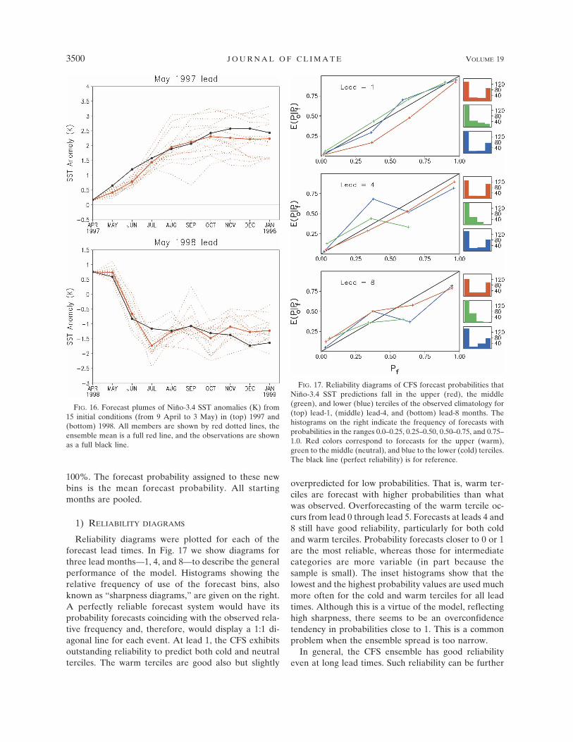
some measures of the performance of the entire en-semble CFS SST forecasts over the Nino-3.4 region. Asan introduction, Fig. 16 shows forecasts by all 15 mem-bers in 1997 and 1998 from May initial conditions.Clearly, not only is the ensemble mean close to theobservation (black line), but the cloud of solutionspractically rules out that the winter 1997/98 (1998/99)
FIG. 11. As in Fig. 10 but for precipitation.
1 AUGUST 2006 S A H A E T A L . 3495
Fig 11 live 4/C
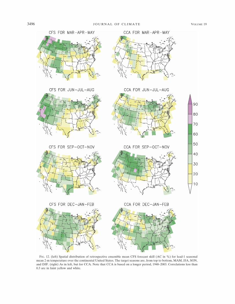
FIG. 12. (left) Spatial distribution of retrospective ensemble mean CFS forecast skill (AC in %) for lead-1 seasonalmean 2-m temperature over the continental United States. The target seasons are, from top to bottom, MAM, JJA, SON,and DJF. (right) As in left, but for CCA. Note that CCA is based on a longer period, 1948–2003. Correlations less than0.3 are in faint yellow and white.
3496 J O U R N A L O F C L I M A T E VOLUME 19
Fig 12 live 4/C
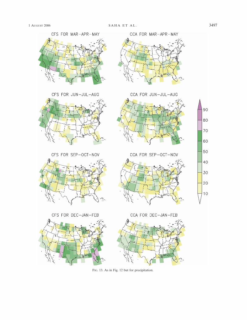
FIG. 13. As in Fig. 12 but for precipitation.
1 AUGUST 2006 S A H A E T A L . 3497
Fig 13 live 4/C
would be anything but a warm (cold) event. These arejust two cases, albeit very strong. The two measuresdiscussed below are to describe probabilistic perfor-mance in general. The first is the reliability diagram,which indicates how forecast probabilities correspond
to the observed relative frequency of the predictedevent. The second measure is the Brier skill score(BSS), which provides a quantitative evaluation: themean square error of the probabilistic forecasts [see,e.g., Wilks (1995) for a description of both measures].
FIG. 14. Anomaly correlation (in %) of ensemble mean CFS forecasts as a function of lead (vertical) and target month (horizontal)for monthly mean 2-m temperature over four quadrants of the continental United States (using 37.5°N and 95°W to define quadrants;see map at the top), evaluated only over those instances during 1981–2003 when an anomaly larger than two standard deviationsoccurred in the observations (anywhere in the quadrant). The much-reduced sample size (relative to Fig. 7) causes noisier patterns.
3498 J O U R N A L O F C L I M A T E VOLUME 19
Fig 14 live 4/C
Probabilistic forecasts can be generated from the en-semble of forecasts by computing the fraction of mem-bers predicting a particular event among all the mem-bers in the ensemble.
BSS is defined as
BSS � 1 �B
Bc,
where B is the Brier score, defined as
B �1N �
i�1
N
�pi � xi�2,
and Bc is the Brier score of a reference, which in thiscase is the observed climatological distribution. Here, pi
is the forecast probability of an “event,” xi is its occur-
rence (1 if it happens and 0 if it does not), and N is thenumber of realizations of the forecast process.
Three events are analyzed: that the SST over Niño-3.4 is in the upper, in the middle, and in the lowertercile of the distribution of the observed climatology,which we refer here to the warm, neutral, and coldterciles, respectively. We first removed the mean sys-tematic error in a “leave-two-years-out” cross-validation manner: of the 23 years of data, 21 were usedto compute the mean systematic error and two wereheld for analysis. Because the length of the retrospec-tive forecast dataset is relatively short, a reduction inthe number of bins was necessary to accumulate alarger sample for each of the bins and produce smoothresults for the reliability diagrams. Probability bins cho-sen are 0%–25%, 25%–50%, 50%–75%, and 75%–
FIG. 15. As in Fig. 14 but for precipitation.
1 AUGUST 2006 S A H A E T A L . 3499
Fig 15 live 4/C
100%. The forecast probability assigned to these newbins is the mean forecast probability. All startingmonths are pooled.
1) RELIABILITY DIAGRAMS
Reliability diagrams were plotted for each of theforecast lead times. In Fig. 17 we show diagrams forthree lead months—1, 4, and 8—to describe the generalperformance of the model. Histograms showing therelative frequency of use of the forecast bins, alsoknown as “sharpness diagrams,” are given on the right.A perfectly reliable forecast system would have itsprobability forecasts coinciding with the observed rela-tive frequency and, therefore, would display a 1:1 di-agonal line for each event. At lead 1, the CFS exhibitsoutstanding reliability to predict both cold and neutralterciles. The warm terciles are good also but slightly
overpredicted for low probabilities. That is, warm ter-ciles are forecast with higher probabilities than whatwas observed. Overforecasting of the warm tercile oc-curs from lead 0 through lead 5. Forecasts at leads 4 and8 still have good reliability, particularly for both coldand warm terciles. Probability forecasts closer to 0 or 1are the most reliable, whereas those for intermediatecategories are more variable (in part because thesample is small). The inset histograms show that thelowest and the highest probability values are used muchmore often for the cold and warm terciles for all leadtimes. Although this is a virtue of the model, reflectinghigh sharpness, there seems to be an overconfidencetendency in probabilities close to 1. This is a commonproblem when the ensemble spread is too narrow.
In general, the CFS ensemble has good reliabilityeven at long lead times. Such reliability can be further
FIG. 16. Forecast plumes of Niño-3.4 SST anomalies (K) from15 initial conditions (from 9 April to 3 May) in (top) 1997 and(bottom) 1998. All members are shown by red dotted lines, theensemble mean is a full red line, and the observations are shownas a full black line.
FIG. 17. Reliability diagrams of CFS forecast probabilities thatNiño-3.4 SST predictions fall in the upper (red), the middle(green), and lower (blue) terciles of the observed climatology for(top) lead-1, (middle) lead-4, and (bottom) lead-8 months. Thehistograms on the right indicate the frequency of forecasts withprobabilities in the ranges 0.0–0.25, 0.25–0.50, 0.50–0.75, and 0.75–1.0. Red colors correspond to forecasts for the upper (warm),green to the middle (neutral), and blue to the lower (cold) terciles.The black line (perfect reliability) is for reference.
3500 J O U R N A L O F C L I M A T E VOLUME 19
Fig 16 live 4/C Fig 17 live 4/C
improved through calibration procedures as has beendone in other ensemble prediction systems (e.g., Zhu etal. 1996; Hamill and Colucci 1998; Raftery et al. 2003;Doblas-Reyes et al. 2005).
2) THE BRIER SKILL SCORE
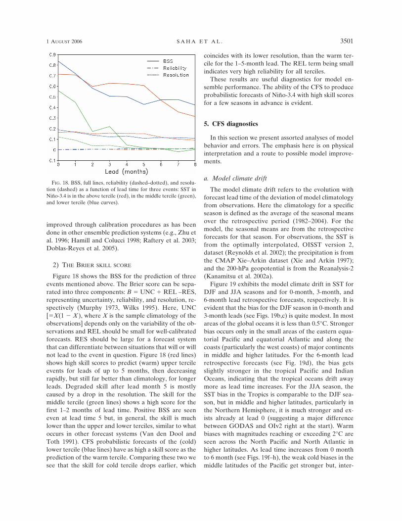
Figure 18 shows the BSS for the prediction of threeevents mentioned above. The Brier score can be sepa-rated into three components: B � UNC � REL –RES,representing uncertainty, reliability, and resolution, re-spectively (Murphy 1973, Wilks 1995). Here, UNC[�X(1 � X), where X is the sample climatology of theobservations] depends only on the variability of the ob-servations and REL should be small for well-calibratedforecasts. RES should be large for a forecast systemthat can differentiate between situations that will or willnot lead to the event in question. Figure 18 (red lines)shows high skill scores to predict (warm) upper tercileevents for leads of up to 5 months, then decreasingrapidly, but still far better than climatology, for longerleads. Degraded skill after lead month 5 is mostlycaused by a drop in the resolution. The skill for themiddle tercile (green lines) shows a high score for thefirst 1–2 months of lead time. Positive BSS are seeneven at lead time 5 but, in general, the skill is muchlower than the upper and lower terciles, similar to whatoccurs in other forecast systems (Van den Dool andToth 1991). CFS probabilistic forecasts of the (cold)lower tercile (blue lines) have as high a skill score as theprediction of the warm tercile. Comparing these two wesee that the skill for cold tercile drops earlier, which
coincides with its lower resolution, than the warm ter-cile for the 1–5-month lead. The REL term being smallindicates very high reliability for all terciles.
These results are useful diagnostics for model en-semble performance. The ability of the CFS to produceprobabilistic forecasts of Niño-3.4 with high skill scoresfor a few seasons in advance is evident.
5. CFS diagnostics
In this section we present assorted analyses of modelbehavior and errors. The emphasis here is on physicalinterpretation and a route to possible model improve-ments.
a. Model climate drift
The model climate drift refers to the evolution withforecast lead time of the deviation of model climatologyfrom observations. Here the climatology for a specificseason is defined as the average of the seasonal meansover the retrospective period (1982–2004). For themodel, the seasonal means are from the retrospectiveforecasts for that season. For observations, the SST isfrom the optimally interpolated, OISST version 2,dataset (Reynolds et al. 2002); the precipitation is fromthe CMAP Xie–Arkin dataset (Xie and Arkin 1997);and the 200-hPa geopotential is from the Reanalysis-2(Kanamitsu et al. 2002a).
Figure 19 exhibits the model climate drift in SST forDJF and JJA seasons and for 0-month, 3-month, and6-month lead retrospective forecasts, respectively. It isevident that the bias for the DJF season in 0-month and3-month leads (see Figs. 19b,c) is quite modest. In mostareas of the global oceans it is less than 0.5°C. Strongerbias occurs only in the small areas of the eastern equa-torial Pacific and equatorial Atlantic and along thecoasts (particularly the west coasts) of major continentsin middle and higher latitudes. For the 6-month leadretrospective forecasts (see Fig. 19d), the bias getsslightly stronger in the tropical Pacific and IndianOceans, indicating that the tropical oceans drift awaymore as lead time increases. For the JJA season, theSST bias in the Tropics is comparable to the DJF sea-son, but in middle and higher latitudes, particularly inthe Northern Hemisphere, it is much stronger and ex-ists already at lead 0 (suggesting a major differencebetween GODAS and OIv2 right at the start). Warmbiases with magnitudes reaching or exceeding 2°C areseen across the North Pacific and North Atlantic inhigher latitudes. As lead time increases from 0 monthto 6 month (see Figs. 19f–h), the weak cold biases in themiddle latitudes of the Pacific get stronger but, inter-
FIG. 18. BSS, full lines, reliability (dashed–dotted), and resolu-tion (dashed) as a function of lead time for three events: SST inNiño-3.4 is in the above tercile (red), in the middle tercile (green),and lower tercile (blue curves).
1 AUGUST 2006 S A H A E T A L . 3501
Fig 18 live 4/C
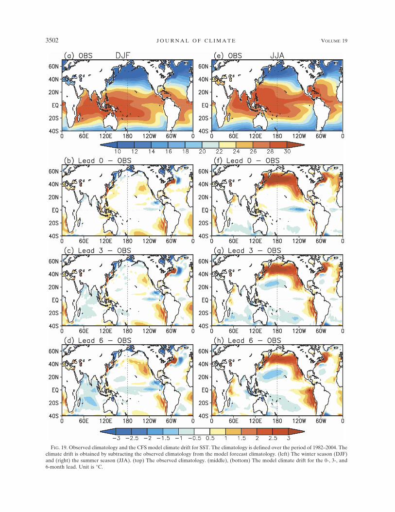
FIG. 19. Observed climatology and the CFS model climate drift for SST. The climatology is defined over the period of 1982–2004. Theclimate drift is obtained by subtracting the observed climatology from the model forecast climatology. (left) The winter season (DJF)and (right) the summer season (JJA). (top) The observed climatology. (middle), (bottom) The model climate drift for the 0-, 3-, and6-month lead. Unit is °C.
3502 J O U R N A L O F C L I M A T E VOLUME 19
Fig 19 live 4/C
estingly, the cold biases in the equatorial Pacific be-comes weaker. The warm biases along the west coastsmay come from the poor parameterization of the strati-form cloud near the cold tongue regions and subtropi-cal highs, a problem in many CGCMs.
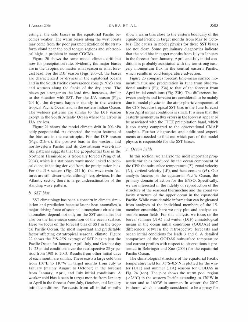
Figure 20 shows the same model climate drift butnow for precipitation rate. Evidently the major biasesare in the Tropics, no matter what season or what fore-cast lead. For the DJF season (Figs. 20b–d), the biasesare characterized by dryness in the equatorial oceansand in the South Pacific convergence zone (SPCZ) areaand wetness along the flanks of the dry areas. Thebiases get stronger as the lead time increases, similarto the situation with SST. For the JJA season (Figs.20f–h), the dryness happens mainly in the westerntropical Pacific Ocean and in the eastern Indian Ocean.The wetness patterns are similar to the DJF seasonexcept in the South Atlantic Ocean where the errors inJJA are less.
Figure 21 shows the model climate drift in 200-hPaeddy geopotential. As expected, the major features ofthe bias are in the extratropics. For the DJF season(Figs. 21b–d), the positive bias in the western andnorthwestern Pacific and its downstream wave-train-like patterns suggests that the geopotential bias in theNorthern Hemisphere is tropically forced (Peng et al.2004), which is a stationary wave mode linked to tropi-cal diabatic heating derived from the precipitation bias.For the JJA season (Figs. 21f–h), the wave train fea-tures are still discernable, although less obvious. In theAtlantic sector, there is large underestimation of thestanding wave pattern.
b. SST bias
SST climatology has been a concern in climate simu-lation and prediction because latent heat anomalies, amajor driving force of seasonal atmospheric circulationanomalies, depend not only on the SST anomalies butalso on the time-mean condition of the ocean surface.Here we focus on the forecast bias of SST in the tropi-cal Pacific Ocean, the most important and predictablefactor affecting extratropical seasonal climate. Figure22 shows the 2°S–2°N average of SST bias in just thePacific Ocean for January, April, July, and October day19–23 initial conditions over the retrospective 23-yr pe-riod from 1981 to 2003. Results from other initial daysof each month are similar. There exists a large cold biasfrom 150°E to 110°W in target months from July toJanuary (mainly August to October) in the forecastfrom January, April, and July initial conditions. Aweaker cold bias is seen in target months from Januaryto April in the forecast from July, October, and Januaryinitial conditions. Forecasts from all initial months
show a warm bias close to the eastern boundary of theequatorial Pacific in target months from May to Octo-ber. The causes in model physics for these SST biasesare not clear. Some preliminary diagnostics indicatethat the cold bias in target months from July to Januaryin the forecast from January, April, and July initial con-ditions is probably associated with the too-strong east-erly momentum flux in the central eastern Pacific,which results in cold temperature advection.
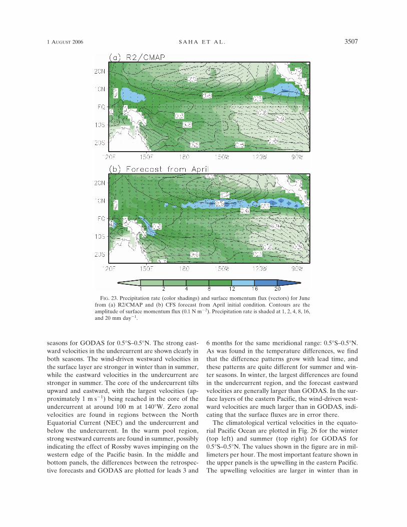
Figure 23 compares forecast time-mean surface mo-mentum flux and precipitation in June from observa-tional analysis (Fig. 23a) to that of the forecast fromApril initial conditions (Fig. 23b). The differences be-tween analysis and forecast are considered to be mainlydue to model physics in the atmospheric component ofthe CFS because tropical SST bias in the June forecastfrom April initial conditions is small. It is seen that theeasterly momentum flux errors in the forecast appear tobe associated with the ITCZ precipitation band, whichis too strong compared to the observational CMAPanalysis. Further diagnostics and additional experi-ments are needed to find out which part of the modelphysics is responsible for the SST biases.
c. Ocean fields
In this section, we analyze the most important prog-nostic variables produced by the ocean component ofthe CFS: the subsurface temperature (T), zonal velocity(U), vertical velocity (W), and heat content (H). Ouranalysis focuses on the equatorial Pacific Ocean, theprimary domain of action for the ENSO. Specifically,we are interested in the fidelity of reproduction of thestructure of the seasonal thermocline and the zonal ve-locity structure of the upper ocean in the equatorialPacific. While considerable information can be gleanedfrom analyses of the individual members of the 15-member ensemble, here we only plot and analyze en-semble mean fields. For this analysis, we focus on theboreal summer (JJA) and winter (DJF) climatologicalmeans in the ocean initial conditions (GODAS) anddifferences between the retrospective forecasts andocean initial conditions for leads 3 and 6. A detailedcomparison of the GODAS subsurface temperatureand current profiles with respect to observations is pre-sented in Behringer and Xue (2004) for the equatorialPacific Ocean.
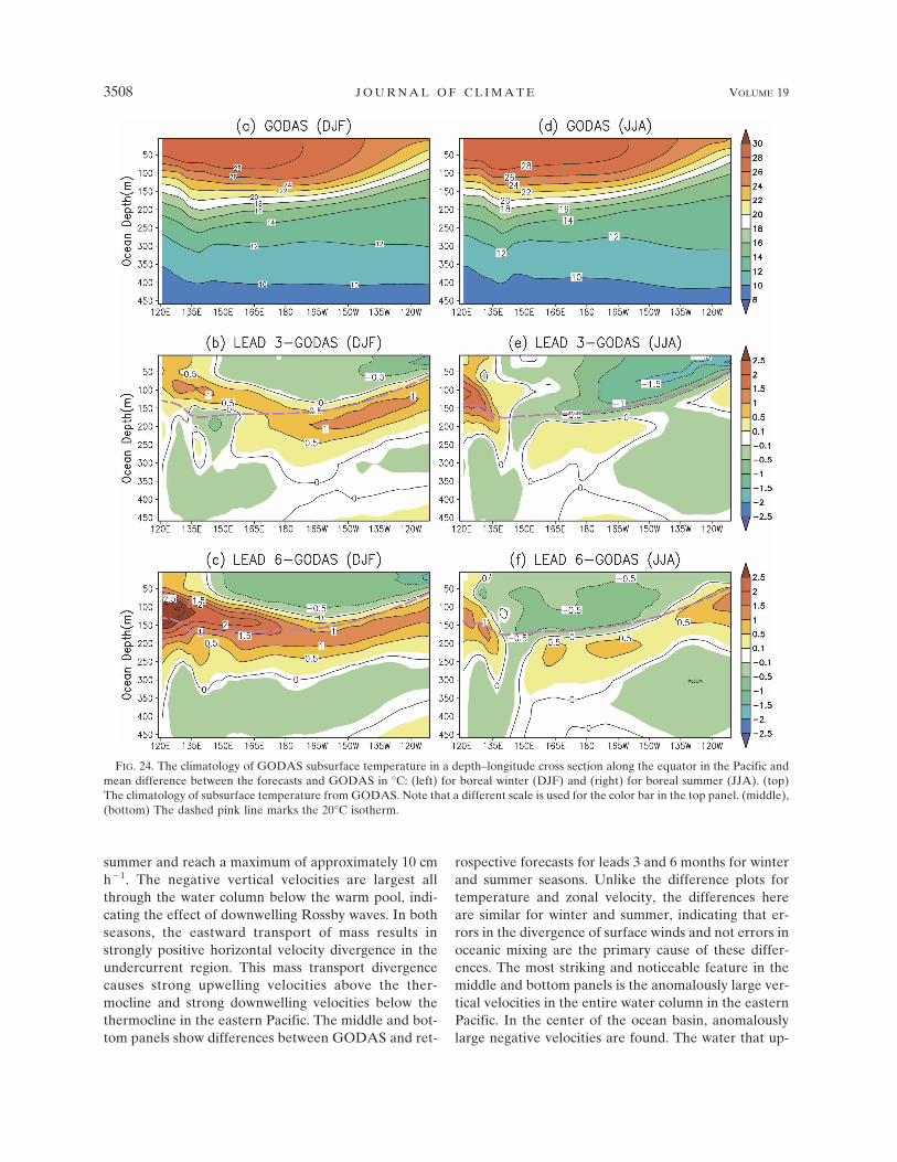
The climatological structure of the equatorial Pacifictemperature field for 0.5°S–0.5°N is plotted for the win-ter (DJF) and summer (JJA) seasons for GODAS inFig. 24 (top). The plot shows the warm pool region(28°C) in the western Pacific extending to 170°W inwinter and to 160°W in summer. In winter, the 20°Cisotherm, which is usually considered to be a proxy for
1 AUGUST 2006 S A H A E T A L . 3503
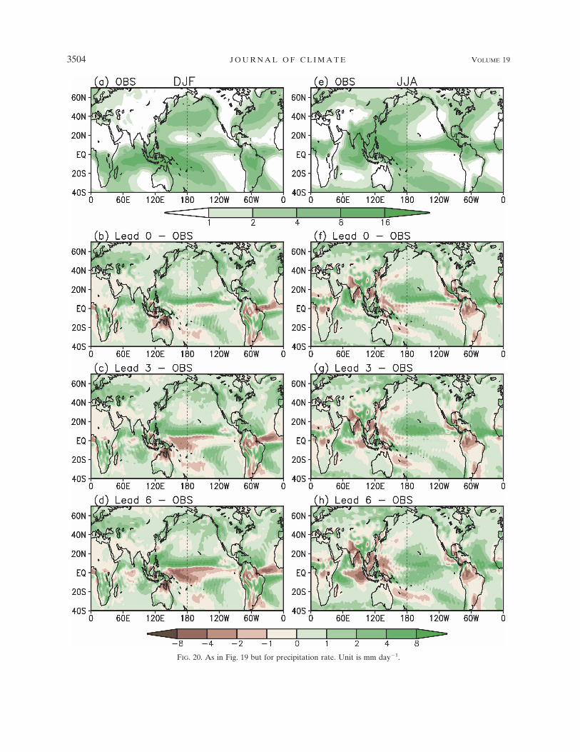
FIG. 20. As in Fig. 19 but for precipitation rate. Unit is mm day�1.
3504 J O U R N A L O F C L I M A T E VOLUME 19
Fig 20 live 4/C
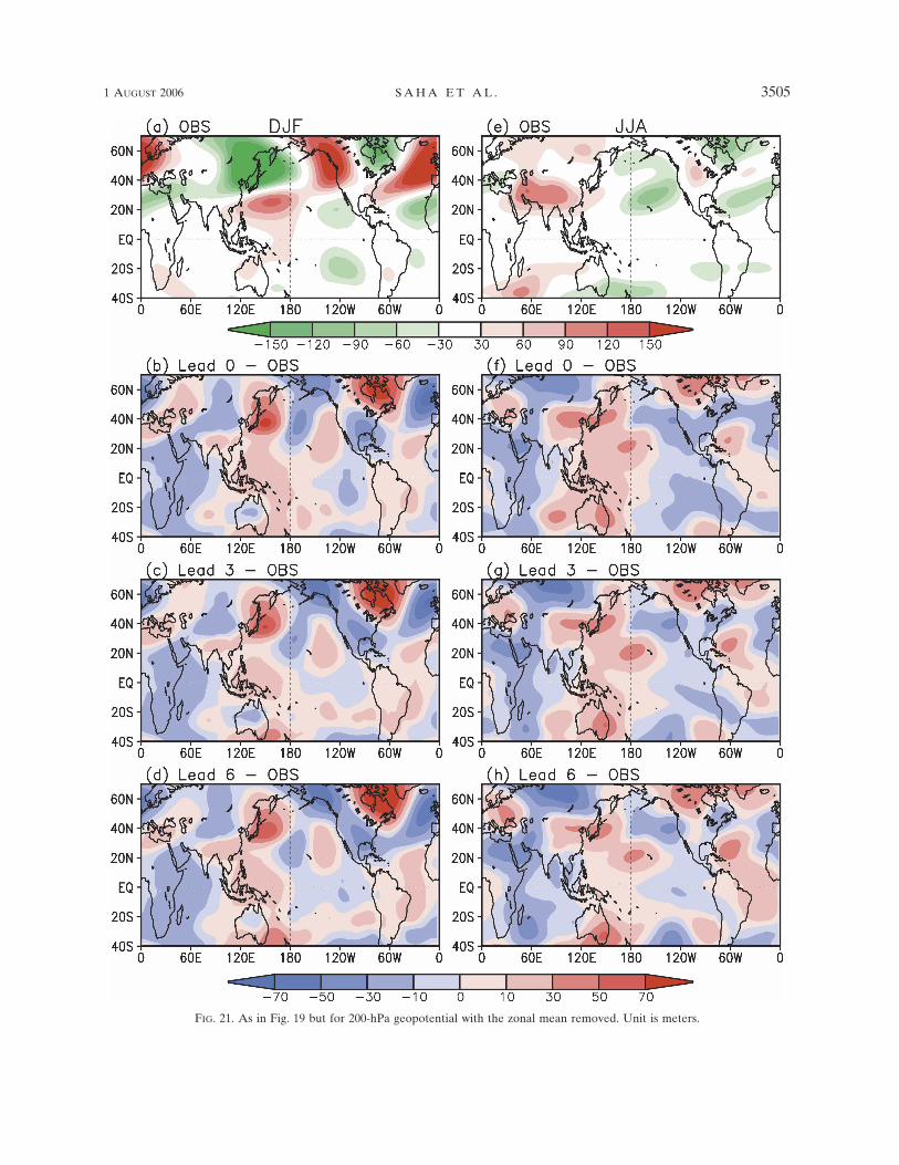
FIG. 21. As in Fig. 19 but for 200-hPa geopotential with the zonal mean removed. Unit is meters.
1 AUGUST 2006 S A H A E T A L . 3505
Fig 21 live 4/C
the depth of the thermocline in the equatorial PacificOcean (McPhaden et al. 1998), shoals from approxi-mately 160 m at its deepest point in the western Pacific(140°E) to 60 m in the eastern Pacific (Nadiga et al.2004). In the summer, the 20°C isotherm is deeper inthe western Pacific than in winter, but the situation isreversed in the eastern Pacific with the shallowestdepths being less than 50 m at the eastern edge of thebasin in summer. In winter, the SSTs are everywherewarmer than 24°C in the equatorial Pacific, but the coldtongue region extends farther west than in summer. Allthese well-known features are well represented in theGODAS. In Fig. 24 (middle and bottom), the differ-ences between the retrospective forecasts and GODASare plotted for winter (left) and summer (right) seasonsfor the same meridional range: 0.5°S–0.5°N. As shownin Fig. 24, the differences are small and typically lessthan 1°C. The greatest differences can be seen justabove and below the seasonal thermocline (a dashedpink line marks the 20°C isotherm in the panels), indi-cating the effects of errors in vertical mixing in theocean model. In GODAS these errors in vertical mix-ing are alleviated by data assimilation. Notice that theretrospective forecasts are typically colder than GODASexcept just above and below the 20°C isotherm. While
the difference pattern grows in amplitude from lead 3to lead 6 for both winter and summer seasons, the dif-ference pattern is quite different for winter and sum-mer. This marked difference between winter and sum-mer difference patterns suggests that the difference pat-terns do not result only from inbuilt trends/errors in theocean model, but are also due to season-dependent er-rors in ocean–atmosphere coupling in the retrospectiveforecasts. In the eastern Pacific, these forecasts areanomalously cold compared to GODAS, and this isbecause of too-strong vertical upwelling in that region.
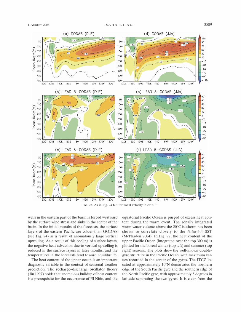
Planetary and Kelvin waves in the equatorial PacificOcean play an important role in setting the period andduration of ENSO events (Schopf and Suarez 1988).The zonal velocities of the planetary and Kelvin wavesare functions of the depth of the thermocline locally,while the amplitudes of the mean zonal currents arefunctions of the slope of the thermocline. This implicitrelationship between the zonal currents and computedtravel times of basin-crossing planetary and Kelvinwaves requires that the mean zonal velocity in the ret-rospective forecasts be examined for any systematic bi-ases when compared to observations. The climatologi-cal zonal velocity in the equatorial Pacific is plotted inFig. 25 for winter (top left) and summer (top right)
FIG. 22. Climate drift (bias) of 2°S–2°N average SSTs in the Pacific for forecast from initial conditions of (a) January, (b) April, (c)July, and (d) October. Contours are drawn at a 0.5-K interval. Negative values are shaded. The SST bias is relative to monthly OIv2fields averaged over 1982–2004.
3506 J O U R N A L O F C L I M A T E VOLUME 19
seasons for GODAS for 0.5°S–0.5°N. The strong east-ward velocities in the undercurrent are shown clearly inboth seasons. The wind-driven westward velocities inthe surface layer are stronger in winter than in summer,while the eastward velocities in the undercurrent arestronger in summer. The core of the undercurrent tiltsupward and eastward, with the largest velocities (ap-proximately 1 m s�1) being reached in the core of theundercurrent at around 100 m at 140°W. Zero zonalvelocities are found in regions between the NorthEquatorial Current (NEC) and the undercurrent andbelow the undercurrent. In the warm pool region,strong westward currents are found in summer, possiblyindicating the effect of Rossby waves impinging on thewestern edge of the Pacific basin. In the middle andbottom panels, the differences between the retrospec-tive forecasts and GODAS are plotted for leads 3 and
6 months for the same meridional range: 0.5°S–0.5°N.As was found in the temperature differences, we findthat the difference patterns grow with lead time, andthese patterns are quite different for summer and win-ter seasons. In winter, the largest differences are foundin the undercurrent region, and the forecast eastwardvelocities are generally larger than GODAS. In the sur-face layers of the eastern Pacific, the wind-driven west-ward velocities are much larger than in GODAS, indi-cating that the surface fluxes are in error there.
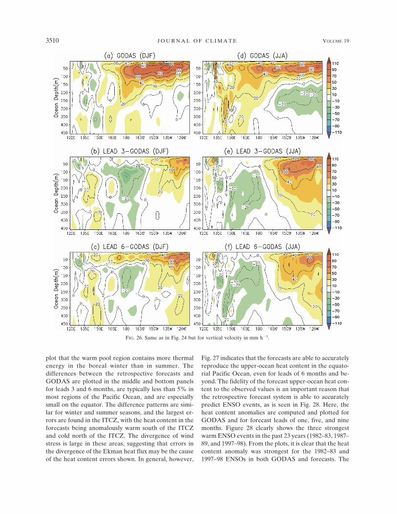
The climatological vertical velocities in the equato-rial Pacific Ocean are plotted in Fig. 26 for the winter(top left) and summer (top right) for GODAS for0.5°S–0.5°N. The values shown in the figure are in mil-limeters per hour. The most important feature shown inthe upper panels is the upwelling in the eastern Pacific.The upwelling velocities are larger in winter than in
FIG. 23. Precipitation rate (color shadings) and surface momentum flux (vectors) for Junefrom (a) R2/CMAP and (b) CFS forecast from April initial condition. Contours are theamplitude of surface momentum flux (0.1 N m�2). Precipitation rate is shaded at 1, 2, 4, 8, 16,and 20 mm day�1.
1 AUGUST 2006 S A H A E T A L . 3507
Fig 23 live 4/C
summer and reach a maximum of approximately 10 cmh�1. The negative vertical velocities are largest allthrough the water column below the warm pool, indi-cating the effect of downwelling Rossby waves. In bothseasons, the eastward transport of mass results instrongly positive horizontal velocity divergence in theundercurrent region. This mass transport divergencecauses strong upwelling velocities above the ther-mocline and strong downwelling velocities below thethermocline in the eastern Pacific. The middle and bot-tom panels show differences between GODAS and ret-
rospective forecasts for leads 3 and 6 months for winterand summer seasons. Unlike the difference plots fortemperature and zonal velocity, the differences hereare similar for winter and summer, indicating that er-rors in the divergence of surface winds and not errors inoceanic mixing are the primary cause of these differ-ences. The most striking and noticeable feature in themiddle and bottom panels is the anomalously large ver-tical velocities in the entire water column in the easternPacific. In the center of the ocean basin, anomalouslylarge negative velocities are found. The water that up-
FIG. 24. The climatology of GODAS subsurface temperature in a depth–longitude cross section along the equator in the Pacific andmean difference between the forecasts and GODAS in °C: (left) for boreal winter (DJF) and (right) for boreal summer (JJA). (top)The climatology of subsurface temperature from GODAS. Note that a different scale is used for the color bar in the top panel. (middle),(bottom) The dashed pink line marks the 20°C isotherm.
3508 J O U R N A L O F C L I M A T E VOLUME 19
Fig 24 live 4/C
wells in the eastern part of the basin is forced westwardby the surface wind stress and sinks in the center of thebasin. In the initial months of the forecasts, the surfacelayers of the eastern Pacific are colder than GODAS(see Fig. 24) as a result of anomalously large verticalupwelling. As a result of this cooling of surface layers,the negative heat advection due to vertical upwelling isreduced in the surface layers in later months, and thetemperatures in the forecasts tend toward equilibrium.
The heat content of the upper ocean is an importantdiagnostic variable in the context of seasonal weatherprediction. The recharge–discharge oscillator theory(Jin 1997) holds that anomalous buildup of heat contentis a prerequisite for the occurrence of El Niño, and the
equatorial Pacific Ocean is purged of excess heat con-tent during the warm event. The zonally integratedwarm water volume above the 20°C isotherm has beenshown to correlate closely to the Niño-3.4 SST(McPhaden 2004). In Fig. 27, the heat content of theupper Pacific Ocean (integrated over the top 300 m) isplotted for the boreal winter (top left) and summer (topright) seasons. The plots show the well-known double-gyre structure in the Pacific Ocean, with maximum val-ues recorded in the center of the gyres. The ITCZ lo-cated at approximately 10°N demarcates the northernedge of the South Pacific gyre and the southern edge ofthe North Pacific gyre, with approximately 5 degrees inlatitude separating the two gyres. It is clear from the
FIG. 25. As in Fig. 24 but for zonal velocity in cm s�1.
1 AUGUST 2006 S A H A E T A L . 3509
Fig 25 live 4/C
plot that the warm pool region contains more thermalenergy in the boreal winter than in summer. Thedifferences between the retrospective forecasts andGODAS are plotted in the middle and bottom panelsfor leads 3 and 6 months, are typically less than 5% inmost regions of the Pacific Ocean, and are especiallysmall on the equator. The difference patterns are simi-lar for winter and summer seasons, and the largest er-rors are found in the ITCZ, with the heat content in theforecasts being anomalously warm south of the ITCZand cold north of the ITCZ. The divergence of windstress is large in these areas, suggesting that errors inthe divergence of the Ekman heat flux may be the causeof the heat content errors shown. In general, however,
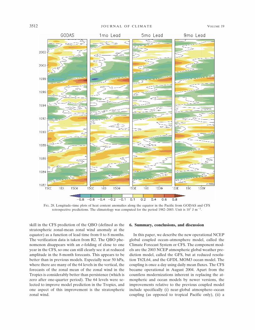
Fig. 27 indicates that the forecasts are able to accuratelyreproduce the upper-ocean heat content in the equato-rial Pacific Ocean, even for leads of 6 months and be-yond. The fidelity of the forecast upper-ocean heat con-tent to the observed values is an important reason thatthe retrospective forecast system is able to accuratelypredict ENSO events, as is seen in Fig. 28. Here, theheat content anomalies are computed and plotted forGODAS and for forecast leads of one, five, and ninemonths. Figure 28 clearly shows the three strongestwarm ENSO events in the past 23 years (1982–83, 1987–89, and 1997–98). From the plots, it is clear that the heatcontent anomaly was strongest for the 1982–83 and1997–98 ENSOs in both GODAS and forecasts. The
FIG. 26. Same as in Fig. 24 but for vertical velocity in mm h�1.
3510 J O U R N A L O F C L I M A T E VOLUME 19
Fig 26 live 4/C
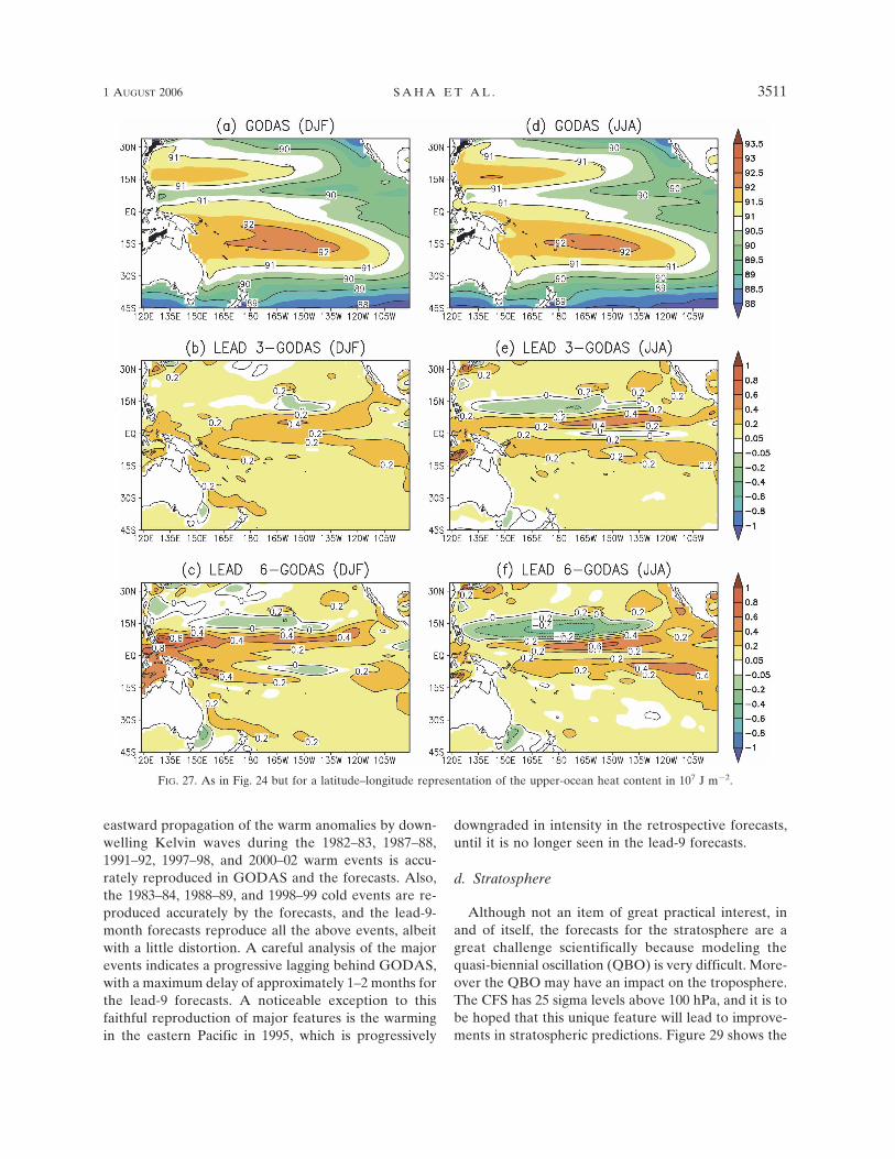
eastward propagation of the warm anomalies by down-welling Kelvin waves during the 1982–83, 1987–88,1991–92, 1997–98, and 2000–02 warm events is accu-rately reproduced in GODAS and the forecasts. Also,the 1983–84, 1988–89, and 1998–99 cold events are re-produced accurately by the forecasts, and the lead-9-month forecasts reproduce all the above events, albeitwith a little distortion. A careful analysis of the majorevents indicates a progressive lagging behind GODAS,with a maximum delay of approximately 1–2 months forthe lead-9 forecasts. A noticeable exception to thisfaithful reproduction of major features is the warmingin the eastern Pacific in 1995, which is progressively
downgraded in intensity in the retrospective forecasts,until it is no longer seen in the lead-9 forecasts.
d. Stratosphere
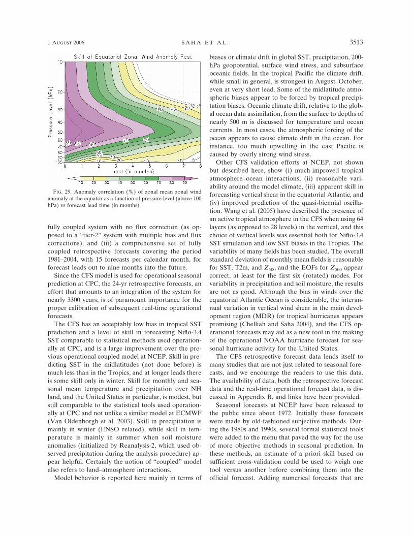
Although not an item of great practical interest, inand of itself, the forecasts for the stratosphere are agreat challenge scientifically because modeling thequasi-biennial oscillation (QBO) is very difficult. More-over the QBO may have an impact on the troposphere.The CFS has 25 sigma levels above 100 hPa, and it is tobe hoped that this unique feature will lead to improve-ments in stratospheric predictions. Figure 29 shows the
FIG. 27. As in Fig. 24 but for a latitude–longitude representation of the upper-ocean heat content in 107 J m�2.
1 AUGUST 2006 S A H A E T A L . 3511
Fig 27 live 4/C
skill in the CFS prediction of the QBO (defined as thestratospheric zonal-mean zonal wind anomaly at theequator) as a function of lead time from 0 to 8 months.The verification data is taken from R2. The QBO phe-nomenon disappears with an e-folding of close to oneyear in the CFS, so one can still clearly see it at reducedamplitude in the 8-month forecasts. This appears to bebetter than in previous models. Especially near 50 hPa,where there are many of the 64 levels in the vertical, theforecasts of the zonal mean of the zonal wind in theTropics is considerably better than persistence (which iszero after one-quarter period). The 64 levels were se-lected to improve model prediction in the Tropics, andone aspect of this improvement is the stratosphericzonal wind.
6. Summary, conclusions, and discussion
In this paper, we describe the new operational NCEPglobal coupled ocean–atmosphere model, called theClimate Forecast System or CFS. The component mod-els are the 2003 NCEP atmospheric global weather pre-diction model, called the GFS, but at reduced resolu-tion T62L64, and the GFDL MOM3 ocean model. Thecoupling is once a day using daily mean fluxes. The CFSbecame operational in August 2004. Apart from thecountless modernizations inherent in replacing the at-mospheric and ocean models by newer versions, theimprovements relative to the previous coupled modelinclude specifically (i) near-global atmosphere–oceancoupling (as opposed to tropical Pacific only), (ii) a
FIG. 28. Longitude–time plots of heat content anomalies along the equator in the Pacific from GODAS and CFSretrospective predictions. The climatology was computed for the period 1982–2003. Unit is 107 J m�2.
3512 J O U R N A L O F C L I M A T E VOLUME 19
Fig 28 live 4/C
fully coupled system with no flux correction (as op-posed to a “tier-2” system with multiple bias and fluxcorrections), and (iii) a comprehensive set of fullycoupled retrospective forecasts covering the period1981–2004, with 15 forecasts per calendar month, forforecast leads out to nine months into the future.
Since the CFS model is used for operational seasonalprediction at CPC, the 24-yr retrospective forecasts, aneffort that amounts to an integration of the system fornearly 3300 years, is of paramount importance for theproper calibration of subsequent real-time operationalforecasts.
The CFS has an acceptably low bias in tropical SSTprediction and a level of skill in forecasting Niño-3.4SST comparable to statistical methods used operation-ally at CPC, and is a large improvement over the pre-vious operational coupled model at NCEP. Skill in pre-dicting SST in the midlatitudes (not done before) ismuch less than in the Tropics, and at longer leads thereis some skill only in winter. Skill for monthly and sea-sonal mean temperature and precipitation over NHland, and the United States in particular, is modest, butstill comparable to the statistical tools used operation-ally at CPC and not unlike a similar model at ECMWF(Van Oldenborgh et al. 2003). Skill in precipitation ismainly in winter (ENSO related), while skill in tem-perature is mainly in summer when soil moistureanomalies (initialized by Reanalysis-2, which used ob-served precipitation during the analysis procedure) ap-pear helpful. Certainly the notion of “coupled” modelalso refers to land–atmosphere interactions.
Model behavior is reported here mainly in terms of
biases or climate drift in global SST, precipitation, 200-hPa geopotential, surface wind stress, and subsurfaceoceanic fields. In the tropical Pacific the climate drift,while small in general, is strongest in August–October,even at very short lead. Some of the midlatitude atmo-spheric biases appear to be forced by tropical precipi-tation biases. Oceanic climate drift, relative to the glob-al ocean data assimilation, from the surface to depths ofnearly 500 m is discussed for temperature and oceancurrents. In most cases, the atmospheric forcing of theocean appears to cause climate drift in the ocean. Forinstance, too much upwelling in the east Pacific iscaused by overly strong wind stress.
Other CFS validation efforts at NCEP, not shownbut described here, show (i) much-improved tropicalatmosphere–ocean interactions, (ii) reasonable vari-ability around the model climate, (iii) apparent skill inforecasting vertical shear in the equatorial Atlantic, and(iv) improved prediction of the quasi-biennial oscilla-tion. Wang et al. (2005) have described the presence ofan active tropical atmosphere in the CFS when using 64layers (as opposed to 28 levels) in the vertical, and thischoice of vertical levels was essential both for Niño-3.4SST simulation and low SST biases in the Tropics. Thevariability of many fields has been studied. The overallstandard deviation of monthly mean fields is reasonablefor SST, T2m, and Z500 and the EOFs for Z500 appearcorrect, at least for the first six (rotated) modes. Forvariability in precipitation and soil moisture, the resultsare not as good. Although the bias in winds over theequatorial Atlantic Ocean is considerable, the interan-nual variation in vertical wind shear in the main devel-opment region (MDR) for tropical hurricanes appearspromising (Chelliah and Saha 2004), and the CFS op-erational forecasts may aid as a new tool in the makingof the operational NOAA hurricane forecast for sea-sonal hurricane activity for the United States.
The CFS retrospective forecast data lends itself tomany studies that are not just related to seasonal fore-casts, and we encourage the readers to use this data.The availability of data, both the retrospective forecastdata and the real-time operational forecast data, is dis-cussed in Appendix B, and links have been provided.
Seasonal forecasts at NCEP have been released tothe public since about 1972. Initially these forecastswere made by old-fashioned subjective methods. Dur-ing the 1980s and 1990s, several formal statistical toolswere added to the menu that paved the way for the useof more objective methods in seasonal prediction. Inthese methods, an estimate of a priori skill based onsufficient cross-validation could be used to weigh onetool versus another before combining them into theofficial forecast. Adding numerical forecasts that are
FIG. 29. Anomaly correlation (%) of zonal mean zonal windanomaly at the equator as a function of pressure level (above 100hPa) vs forecast lead time (in months).
1 AUGUST 2006 S A H A E T A L . 3513
Fig 29 live 4/C
accompanied by appreciable a priori skill is a logicalextension of this procedure. These forecasts may, ormay not, have become much better, but we do have amore representative measure of a priori skill, which isvital for the proper utility of seasonal forecasts.
Acknowledgments. The authors would like to recog-nize all the scientists and technical staff of the GlobalClimate and Weather Modeling Branch of EMC fortheir hard work and dedication to the development andimplementation of the GFS. We would also like to ex-press our thanks to the scientists at GFDL for theirwork in developing the MOM3 ocean model. We thankJulia Zhu, Dave Michaud, Brent Gordon, and SteveGilbert from the NCEP Central Operations (NCO) forthe timely implementation of the CFS in August 2004.George VandenBerghe and Carolyn Pasti from IBM
are recognized for their critical support in the smoothrunning of the CFS retrospective forecasts and the op-erational implementation of the CFS on the NCEPIBM computers. We thank Curtis Marshall, EMC, forhis help in the editing of the manuscript and Åke Jo-hansson and Augustin Vintzileos for constructive inter-nal reviews. Finally, we thank the NOAA Office ofGlobal Programs for the funds to obtain extra comput-ing resources, which enabled us to complete the retro-spective forecasts in a timely fashion.
APPENDIX A
Anomaly Correlation, Systematic Error Correction,and Cross Validation
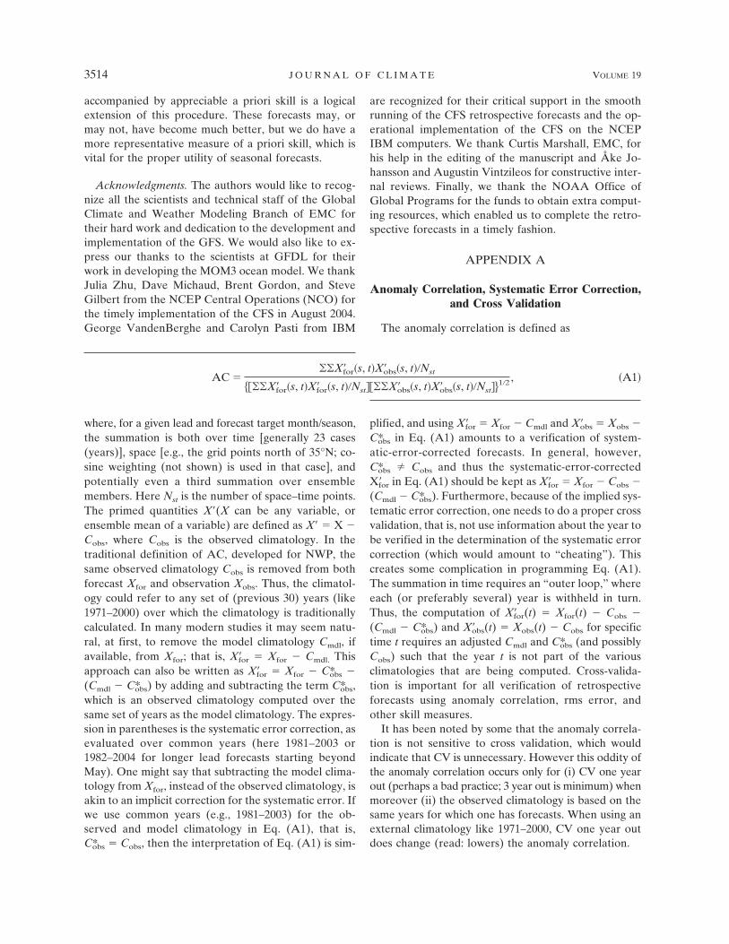
The anomaly correlation is defined as
AC ���X�for�s, t�X�obs�s, t��Nst
���X�for�s, t�X�for�s, t��Nst����X�obs�s, t�X�obs�s, t��Nst� 1�2 , �A1�
where, for a given lead and forecast target month/season,the summation is both over time [generally 23 cases(years)], space [e.g., the grid points north of 35°N; co-sine weighting (not shown) is used in that case], andpotentially even a third summation over ensemblemembers. Here Nst is the number of space–time points.The primed quantities X�(X can be any variable, orensemble mean of a variable) are defined as X� � X �Cobs, where Cobs is the observed climatology. In thetraditional definition of AC, developed for NWP, thesame observed climatology Cobs is removed from bothforecast Xfor and observation Xobs. Thus, the climatol-ogy could refer to any set of (previous 30) years (like1971–2000) over which the climatology is traditionallycalculated. In many modern studies it may seem natu-ral, at first, to remove the model climatology Cmdl, ifavailable, from Xfor; that is, X�for � Xfor � Cmdl. Thisapproach can also be written as X�for � Xfor � C*obs �(Cmdl � C*obs) by adding and subtracting the term C*obs,which is an observed climatology computed over thesame set of years as the model climatology. The expres-sion in parentheses is the systematic error correction, asevaluated over common years (here 1981–2003 or1982–2004 for longer lead forecasts starting beyondMay). One might say that subtracting the model clima-tology from Xfor, instead of the observed climatology, isakin to an implicit correction for the systematic error. Ifwe use common years (e.g., 1981–2003) for the ob-served and model climatology in Eq. (A1), that is,C*obs � Cobs, then the interpretation of Eq. (A1) is sim-
plified, and using X�for � Xfor � Cmdl and X�obs � Xobs �C*obs in Eq. (A1) amounts to a verification of system-atic-error-corrected forecasts. In general, however,C*obs � Cobs and thus the systematic-error-correctedX�for in Eq. (A1) should be kept as X�for � Xfor � Cobs �(Cmdl � C*obs). Furthermore, because of the implied sys-tematic error correction, one needs to do a proper crossvalidation, that is, not use information about the year tobe verified in the determination of the systematic errorcorrection (which would amount to “cheating”). Thiscreates some complication in programming Eq. (A1).The summation in time requires an “outer loop,” whereeach (or preferably several) year is withheld in turn.Thus, the computation of X�for(t) � Xfor(t) � Cobs �(Cmdl � C*obs) and X�obs(t) � Xobs(t) � Cobs for specifictime t requires an adjusted Cmdl and C*obs (and possiblyCobs) such that the year t is not part of the variousclimatologies that are being computed. Cross-valida-tion is important for all verification of retrospectiveforecasts using anomaly correlation, rms error, andother skill measures.
It has been noted by some that the anomaly correla-tion is not sensitive to cross validation, which wouldindicate that CV is unnecessary. However this oddity ofthe anomaly correlation occurs only for (i) CV one yearout (perhaps a bad practice; 3 year out is minimum) whenmoreover (ii) the observed climatology is based on thesame years for which one has forecasts. When using anexternal climatology like 1971–2000, CV one year outdoes change (read: lowers) the anomaly correlation.
3514 J O U R N A L O F C L I M A T E VOLUME 19
APPENDIX B
Operational Forecasts and Availability ofCFS Data
The initial operational implementation of CFS in-volved implementation of three components: R2-baseddaily atmospheric data assimilation, a daily globalocean data assimilation, and a daily 9-month-longcoupled model integration. The retrospective forecastswith the coupled model (discussed in the preceding sec-tions) use R2 analysis–based atmospheric initial statesand R2 analysis–driven assimilated global ocean states.This required NCEP to make R2 atmospheric analysisoperational because it is needed for both the oceananalysis and as initial condition for the CFS forecasts.This real-time operational analysis is called ClimateData Assimilation System 2 (CDAS2).
The operational GODAS uses a 28-day data windowsymmetrically centered on the analysis time. Thus theanalysis date is 14 days behind real time. So, if theGODAS analysis were to be used as the initial condi-tion, then the daily CFS forecasts would be 14 daysbehind real time, which would be unacceptable. There-fore, a new asymmetric GODAS that uses only 21 daysof ocean data and is valid at 7 days prior to real timewas developed and implemented. This asymmetricGODAS uses the previous 28-day symmetric GODASanalysis as its first guess.
Thus, operationally three analyses are performeddaily in real time: the atmospheric R2 analysis is per-formed with analysis time that is 3 days before realtime, the full symmetric GODAS is performed withanalysis time that is 14 days before real time, and anasymmetric GODAS is performed with analysis timethat is 7 days before real time. Using this asymmetricGODAS analysis as the ocean initial state and R2analysis valid at that time as the atmospheric state (at0000 UTC), a daily CFS forecast is made out to 9–10months lead time. An additional daily CFS forecastwith the same initial oceanic state and a slightly per-turbed atmospheric state (by taking a weighted mean ofthe states corresponding to the real-time date and a dayearlier at 0000 UTC) is also now operational. In all,there is at least a 60-member ensemble of CFS forecastsper month.
Monthly means of all variables and daily time seriesof selected variables are being archived from theseforecasts. The retrospective forecasts may be used tocorrect the systematic bias from the operational fore-casts before they are used in a predictive environment.
The official CFS Web site (http://cfs.ncep.noaa.gov)provides necessary details on how to access the opera-tional CFS forecast and retrospective data.
REFERENCES
Anderson, D. L. T., and Coauthors, 2003: Comparison of theECMWF seasonal forecast systems 1 and 2, including therelative performance for the 1997/8 El Niño. Tech. Memo.404, ECMWF, Reading, United Kingdom, 93 pp.
Barnston, A. G., 1994: Linear statistical short-term climate pre-dictive skill in the Northern Hemisphere. J. Climate, 7, 1513–1564.
——, and C. F. Ropelewski, 1992: Prediction of ENSO episodesusing canonical correlation analysis. J. Climate, 5, 1316–1345.
——, and Coauthors, 1994: Long-lead seasonal forecasts—Wheredo we stand? Bull. Amer. Meteor. Soc., 75, 2097–2114.
——, A. Leetmaa, V. Kousky, R. Livezey, E. O’Lenic, H. Van denDool, A. J. Wagner, and D. Unger, 1999: NCEP forecasts ofthe El Niño of 1997–98 and its U.S. impacts. Bull. Amer.Meteor. Soc., 80, 1829–1852.
——, S. J. Mason, L. Goddard, D. G. DeWitt, and S. E. Zebiak,2003: Multimodel ensembling in seasonal climate forecastingat IRI. Bull. Amer. Meteor. Soc., 84, 1783–1796.
Behringer, D. W., and Y. Xue, 2004: Evaluation of the globalocean data assimilation system at NCEP: The Pacific Ocean.Preprints, Eighth Symp. on Integrated Observing and Assimi-lation Systems for Atmosphere, Oceans, and Land Surface,Seattle, WA, Amer. Meteor. Soc., 11–15.
——, M. Ji, and A. Leetmaa, 1998: An improved coupled modelfor ENSO prediction and implications for ocean initializa-tion. Part I: The ocean data assimilation system. Mon. Wea.Rev., 126, 1013–1021.
Chelliah, M., and S. Saha, 2004: Dynamical forecasts of atmo-spheric conditions associated with North Atlantic hurricaneactivity by the Coupled Forecast System at NCEP. Proc. 29thClimate Prediction and Diagnostics Workshop, Madison, WI,NOAA. [Available online at http://www.cpc.ncep.noaa.gov/products/outreach/proceedings/cdw29_proceedings/presentations.shtml.]
Derber, J. D., and A. Rosati, 1989: A global oceanic data assimi-lation system. J. Phys. Oceanogr., 19, 1333–1347.
Doblas-Reyes, F. J., R. Hagedorn, and T. N. Palmer, 2005: Therationale behind the success of multi-model ensembles in sea-sonal forecasting—II: Calibration and combination. Tellus,57A, 234–252.
Fan, Y., and H. van den Dool, 2004: Climate Prediction Centerglobal monthly soil moisture data set at 0.5° resolution for1948 to present. J. Geophys. Res., 109, D10102, doi:10.1029/2003JD004345.
Gent, P. R., and J. C. McWilliams, 1990: Isopycnal mixing inocean circulation models. J. Phys. Oceanogr., 20, 150–155.
Gordon, C., C. Cooper, C. A. Senior, H. T. Banks, J. M. Gregory,T. C. Johns, J. F. B. Mitchell, and R. A. Wood, 2000: Simu-lation of SST, sea ice extents and ocean heat transports in aversion of the Hadley Centre coupled model without fluxadjustments. Climate Dyn., 16, 147–168.
Griffies, S. M., A. Gnanadesikan, R. C. Pacanowski, V. Larichev,J. K. Dukowicz, and R. D. Smith, 1998: Isoneutral diffusionin a z-coordinate ocean model. J. Phys. Oceanogr., 28, 805–830.
Gutman, N. B., and R. G. Quayle, 1996: A historical perspectiveof U.S. climate divisions. Bull. Amer. Meteor. Soc., 77, 293–303.
Hamill, T., and S. J. Colucci, 1998: Evaluation of Eta–RSM en-semble probabilistic precipitation forecasts. Mon. Wea. Rev.,126, 711–724.
1 AUGUST 2006 S A H A E T A L . 3515
Hong, S.-Y., and H.-L. Pan, 1996: Nonlocal boundary layer ver-tical diffusion in a medium-range forecast model. Mon. Wea.Rev., 124, 2322–2339.
——, and ——, 1998: Convective trigger function for a mass-fluxcumulus parameterization scheme. Mon. Wea. Rev., 126,2599–2620.
Hou, Y.-T., K. A. Campana, and S.-K. Yang, 1996: Shortwaveradiation calculations in the NCEP’s global model. IRS ’96:Current Problems in Atmospheric Radiation—Proceedings ofthe International Radiation Symposium, W. L. Smith and K.Stamnes, Eds., A. Deepak Publishing, 317–319.
——, S. Moorthi, and K. Campana, 2002: Parameterization ofsolar radiation transfer in the NCEP models. NCEP OfficeNote 441, 34 pp. [Available online at http://www.emc.ncep.noaa.gov/officenotes/FullTOC.html#2000.]
Ji, M., A. Kumar, and A. Leetmaa, 1994: A multiseason climateforecast system at the National Meteorological Center. Bull.Amer. Meteor. Soc., 75, 569–578.
——, A. Leetmaa, and J. Derber, 1995: An ocean analysis systemfor seasonal to interannual climate studies. Mon. Wea. Rev.,123, 460–481.
——, D. W. Behringer, and A. Leetmaa, 1998: An improvedcoupled model for ENSO prediction and implications forocean initialization. Part II: The coupled model. Mon. Wea.Rev., 126, 1022–1034.
——, R. Reynolds, and D. W. Behringer, 2000: Use of TOPEX/Poseidon sea level data for ocean analyses and ENSO pre-diction: Some early results. J. Climate, 13, 216–231.
Jin, F.-F., 1997: An equatorial recharge paradigm for ENSO. PartI: Conceptual model. J. Atmos. Sci., 54, 811–829.
Kalnay, E., and Coauthors, 1996: The NCEP/NCAR 40-Year Re-analysis Project. Bull. Amer. Meteor. Soc., 77, 437–471.
Kanamitsu, M., W. Ebisuzaki, J. Woollen, S.-K. Yang, J. J. Hnilo,M. Fiorino, and G. L. Potter, 2002a: NCEP–DOE AMIP-IIReanalysis (R-2). Bull. Amer. Meteor. Soc., 83, 1631–1643.
——, and Coauthors, 2002b: NCEP dynamical seasonal forecastsystem 2000. Bull. Amer. Meteor. Soc., 83, 1019–1037.
Kim, Y.-J. and A. Arakawa, 1995: Improvement of orographicgravity wave parameterization using a mesoscale gravitywave model. J. Atmos. Sci., 52, 1875–1902.
Kirtman, B. P., 2003: The COLA anomaly coupled model: En-semble ENSO prediction. Mon. Wea. Rev., 131, 2324–2341.
Kistler, R. E., and Coauthors, 2001: The NCEP–NCAR 50-yearreanalysis: Monthly means CD-ROM and documentation.Bull. Amer. Meteor. Soc., 82, 247–268.
Large, W. G., J. C. McWilliams, and S. C. Doney, 1994: Oceanicvertical mixing: A review and a model with nonlocal bound-ary layer parameterization. Rev. Geophys., 32, 363–403.
Levitus, S., R. Burgett, and T. P. Boyer, 1994: Salinity. Vol. 3,World Ocean Atlas 1994, NOAA Atlas NESDIS 3, 99 pp.
Leith, C. E., 1974: Theoretical skill of Monte Carlo forecasts.Mon. Wea. Rev., 102, 409–418.
Maes, C., and D. Behringer, 2000: Using satellite-derived sea leveland temperature profiles for determining the salinity variabil-ity: A new approach. J. Geophys. Res., 105 (C4), 8537–8547.
Mahrt, L., and H.-L. Pan, 1984: A two-layer model of soil hydrol-ogy. Bound.-Layer Meteor., 29, 1–20.
Manabe, S., and K. Bryan, 1969: Climate calculations with a com-bined ocean-atmosphere model. J. Atmos. Sci., 26, 786–789.
McPhaden, M. J., 2004: Evolution of the 2002/03 El Niño. Bull.Amer. Meteor. Soc., 85, 677–695.
——, and Coauthors, 1998: The Tropical Ocean Global Atmo-
spheric (TOGA) observing system: A decade of progress. J.Geophys. Res., 103 (C7), 14 169–14 240.
Moorthi, S., H.-L. Pan, and P. Caplan, 2001: Changes to the 2001NCEP operational MRF/AVN global analysis/forecast sys-tem. NWS Tech. Procedures Bulletin 484, 14 pp. [Availableonline at http://www.nws.noaa.gov/om/tpb/484.htm.]
Murphy, A. H., 1973: A new vector partition of the probabilityscore. J. Appl. Meteor., 12, 595–600.
Nadiga, S., J. Wang, D. Behringer, and S. Saha, 2004: Ocean ret-rospective forecasts from the new coupled forecast system:1981–2003. Proc. 29th Climate Prediction and DiagnosticsWorkshop, Madison, WI, NOAA. [Available online at http://www.cpc.ncep.noaa.gov/products/outreach/proceedings/cdw29_proceedings/presentations.shtml.]
Pacanowski, R. C., and S. M. Griffies, cited 1998: MOM 3.0manual. NOAA/GFDL. [Available online at http://www.gfdl.noaa.gov/�smg/MOM/web/guide_parent/guide_parent.html.]
Palmer, T. N., and Coauthors, 2004: Development of a EuropeanMultimodel Ensemble System for Seasonal-to-InterannualPrediction (DEMETER). Bull. Amer. Meteor. Soc., 85, 853–872.
Peng, P., A. Kumar, H. van den Dool, and A. G. Barnston, 2002:An analysis of multimodel ensemble predictions for seasonalclimate anomalies. J. Geophys. Res., 107, 4710, doi:10.1029/2002JD002712.
——, Q. Zhang, A. Kumar, H. van den Dool, W. Wang, S. Saha,and H.-L. Pan, 2004: Variability, predictability and predictionof DJF season climate in CFS. Proc. 29th Climate Predictionand Diagnostics Workshop, Madison, WI, NOAA. [Availableonline at http://www.cpc.ncep.noaa.gov/products/outreach/proceedings/cdw29_proceedings/presentations.shtml.]
Pope, V. D., M. L. Gallani, P. R. Rowntree, and R. A. Stratton,2000: The impact of new physical parametrizations in theHadley Centre climate model—HadAM3. Climate Dyn., 16,123–146.
Raftery, A. E., F. Balabdaoui, T. Gneiting, and M. Polakowski,2003: Using Bayesian model averaging to calibrate forecastensembles. Tech. Rep. 440, Department of Statistics, Univer-sity of Washington, 28 pp. [Available online at www.stat.washington.edu/tech.reports.]
Reynolds, R. W., N. A. Rayner, T. M. Smith, D. C. Stokes, and W.Wang, 2002: An improved in situ and satellite SST analysisfor climate. J. Climate, 15, 1609–1625.
Saha, S., 2004: Validation of the NCEP CFS forecasts. Proc. 29thClimate Prediction and Diagnostics Workshop, Madison, WI,NOAA. [Available online at http://www.cpc.ncep.noaa.gov/products/outreach/proceedings/cdw29_proceedings/presentations.shtml.]
Schneider, E. K., D. G. DeWitt, A. Rosati, B. P. Kirtman, L. Ji,and J. J. Tribbia, 2003: Retrospective ENSO forecasts: Sen-sitivity to atmospheric model and ocean resolution. Mon.Wea. Rev., 131, 3038–3060.
Schopf, P. S., and M. J. Suarez, 1988: Vacillations in a coupledocean–atmosphere model. J. Atmos. Sci., 45, 549–566.
Smagorinsky, J., 1963: General circulation experiments with theprimitive equations: I. The basic experiment. Mon. Wea.Rev., 91, 99–164.
Stockdale, T. N., D. L. T. Anderson, J. O. S. Alves, and M. A.Balmaseda, 1998: Global seasonal rainfall forecasts using acoupled ocean–atmosphere model. Nature, 392, 370–373.
Sundqvist, H., E. Berge, and J. E. Kristjansson, 1989: Condensa-
3516 J O U R N A L O F C L I M A T E VOLUME 19
tion and cloud studies with a mesoscale numerical weatherprediction model. Mon. Wea. Rev., 117, 1641–1657.
Unger, D., A. Barnston, H. Van den Dool, and V. Kousky, 1996:Consolidated forecasts of tropical Pacific SST in Niño 3.4using two dynamical models and two statistical models. Exp.Long-Lead Forecast Bull., 5, 50–52.
Van den Dool, H. M., 1994: Searching for analogues, how longmust one wait? Tellus, 46A, 314–324.
——, and Z. Toth, 1991: Why do forecasts for “near normal” oftenfail? Wea. Forecasting, 6, 76–85.
——, and A. G. Barnston, 1994: Forecasts of global sea surfacetemperature out to a year using the constructed analoguemethod. Proc. 19th Climate Diagnostics Workshop, CollegePark, MD, NOAA, 416–419.
——, and L. Rukhovets, 1994: On the weights for an ensembleaveraged 6–10-day forecast at NMC. Wea. Forecasting, 9,457–465.
Van Oldenborgh, G. J., M. A. Balmaseda, L. Ferranti, T. N.Stockdale, and D. L. T. Anderson, 2003: Did the ECMWFseasonal forecast model outperform a statistical model overthe last 15 years? ECMWF Tech. Memo. 418, 32 pp.
Wang, G., R. Kleeman, N. Smith, and F. Tseitkin, 2002: TheBMRC coupled general circulation model ENSO forecastsystem. Mon. Wea. Rev., 130, 975–991.
Wang, W., S. Saha, H.-L. Pan, S. Nadiga, and G. White, 2005:Simulation of ENSO in the new NCEP Coupled ForecastSystem Model. Mon. Wea. Rev., 133, 1574–1593.
Wilks, D. S., 1995: Statistical Methods in the Atmospheric Sciences:An Introduction. Academic Press, 467 pp.
Xie, P., and P. A. Arkin, 1997: Global precipitation: A 17-yearmonthly analysis based on gauge observations, satellite esti-mates, and numerical model outputs. Bull. Amer. Meteor.Soc., 78, 2539–2558.
Xue, Y., A. Leetmaa, and M. Ji, 2000: ENSO prediction withMarkov models: The impact of sea level. J. Climate, 13, 849–871.
Zhao, Q. Y., and F. H. Carr, 1997: A prognostic cloud scheme foroperational NWP models. Mon. Wea. Rev., 125, 1931–1953.
Zhu, Y., G. Yyengar, Z. Toth, S. M. Tracton, and T. Marchok,1996: Objective evaluation of the NCEP global ensembleforecasting system. Preprints, 15th Conf. on Weather Analysisand Forecasting, Norfolk, VA, Amer. Meteor. Soc., J79–J82.
1 AUGUST 2006 S A H A E T A L . 3517