The NCEP Climate Forecast System Version 2

(http://cfs.ncep.noaa.gov)

Suranjana Saha1, Shrinivas Moorthi

1, Xingren Wu

2, Jiande Wang

4, Sudhir Nadiga

2, Patrick

Tripp2, David Behringer

1, Yu-Tai Hou

1, Hui-ya Chuang

1, Mark Iredell

1, Michael Ek

1, Jesse

Meng2, Rongqian Yang

2, Malaquías Peña Mendez

2, Huug van den Dool

3, Qin Zhang

3, Wanqiu

Wang3, Mingyue Chen

3 and Emily Becker

5

Submitted to the Journal of Climate

Original submission: November 23, 2012

Revised: May 20, 2013

1

Environmental Modeling Center, NCEP/NWS/NOAA, USA. 2

I. M. Systems Group, Inc., USA. 3

Climate Prediction Center, NCEP/NWS/NOAA, USA. 4

Science Systems and Applications, Inc., USA 5 Wyle Lab, Inc., USA.

Corresponding Author: Dr. Suranjana Saha,

NOAA Center for Weather and Climate Prediction (NCWCP)

5830 University Research Court, College Park, MD 20740, USA

Suranjana.Saha@noaa.gov

Abstract 1

The second version of the NCEP Climate Forecast System (CFSv2) was made operational at 2

NCEP in March 2011. This version has upgrades to nearly all aspects of the data assimilation 3

and forecast model components of the system. A coupled Reanalysis was made over a 32 4

year period (1979-2011), which provided the initial conditions to carry out a comprehensive 5

Reforecast over 29 years (1982-2011). This was done to obtain consistent and stable 6

calibrations, as well as, skill estimates for the operational sub seasonal and seasonal 7

predictions at NCEP with CFSv2. The operational implementation of the full system ensures 8

a continuity of the climate record and provides a valuable up-to-date dataset to study many 9

aspects of predictability on the seasonal and sub seasonal scales. Evaluation of the reforecasts 10

show that the CFSv2 increases the length of skillful MJO forecasts from 6 to 17 days 11

(dramatically improving sub-seasonal forecasts), nearly doubles the skill of seasonal 12

forecasts of 2 meter temperatures over the U.S. and significantly improves global SST 13

forecasts over its predecessor. The CFSv2 not only provides greatly improved guidance at 14

these time scales, it also creates many more products for sub-seasonal and seasonal 15

forecasting with an extensive set of retrospective forecasts for users to calibrate their forecast 16

products. These retrospective and real time operational forecasts will be used by a wide 17

community of users in their decision making processes in areas such as water management 18

for rivers and agriculture, transportation, energy use by utilities, wind and other sustainable 19

energy, and seasonal prediction of the hurricane season. 20

21

3

1. Introduction 1

In this paper, we describe the development of NCEP‟s Climate Forecast System version 2 2

(CFSv2). We intend to be fairly complete about this development and the generation of its 3

retrospective data. We also present some limited analysis of the performance of CFSv2. 4

The first CFS, retroactively called CFSv1, was implemented into operations at NCEP in 5

August 2004 and was the first quasi-global, fully coupled atmosphere- ocean-land model 6

used at NCEP for seasonal prediction (Saha et al.,2006, hereafter referred to as S06). Earlier 7

coupled models at NCEP had full ocean coupling restricted to only the tropical Pacific 8

Ocean. CFSv1 was developed from four independently designed pieces of technology, 9

namely the R2 NCEP/DOE Global Reanalysis (Kanamitsu et al., 2002) which provided the 10

atmospheric and land surface initial conditions, a global ocean data assimilation system 11

(GODAS) operational at NCEP in 2003 (Behringer, 2007) which provided the ocean initial 12

states, NCEP‟s Global Forecast System (GFS) operational in 2003 which was the 13

atmospheric model run at a lower resolution of T62L64, and the MOM3 ocean forecast 14

model from GFDL. The CFSv1 system worked well enough that it became difficult to 15

terminate it, as it was used by many in the community, even after the CFSv2 was 16

implemented into operations in March 2011. It was finally decommissioned in late 17

September 2012. 18

Obviously CFSv2 has improvements in all four components mentioned above, namely 19

the two forecast models and the two data assimilation systems. CFSv2 also has a few 20

novelties: an upgraded four level soil model, an interactive three layer sea-ice model, and 21

historical prescribed (i.e. rising) CO2 concentrations. But above all, CFSv2 was designed to 22

4

improve consistency between the model states and the initial states produced by the data 1

assimilation system. It took nearly seven years to complete the following aspects: 2

(1) Carry out extensive testing of a new atmosphere-ocean-sea-ice-land model configuration 3

including decisions on resolution, etc; 4

(2) Make a coupled atmosphere-ocean-seaice-land Reanalysis from 1979-2011 with the new 5

system (resulting in the Climate Forecast System Reanalysis, CFSR) for the purpose of 6

creating initial conditions for CFSv2 retrospective forecasts; 7

(3) Make retrospective forecasts with the new system using initial states from CFSR from 8

1982-2011 and onward to calibrate operational subsequent real time subseasonal and 9

seasonal predictions; 10

(4) Operational implementation of CFSv2. 11

Items (1) and (2) have already been described in Saha et al., 2010, and aspect (4) does not need 12

to be treated in any great detail in a scientific paper, other than to mention that CFSv2 is run in 13

near real time with a very short data cut-off time, thereby increasing its applicability to the 14

shorter time scales relative to CFSv1, which was late by about 36 hours after real time. So, in 15

this paper, we mainly describe the CFSv2 model, the design of the retrospective forecasts, and 16

some results from these forecasts. 17

The performance of the CFSv2 retrospective forecasts can be split into four time scales. 18

The shortest time scale of interest is the subseasonal, mainly geared towards the 19

prediction of the Madden Julian Oscillation (MJO) and more generally forecasts for the 20

week 2 to week 6 period over the United States (or any other part of the globe). 21

The next time scale is the „long-lead‟ seasonal prediction, out to 9 months, for which 22

these systems are ostensibly designed. For both the subseasonal and seasonal, we have a 23

5

very precise comparison between skill of prediction by the CFSv1 and CFSv2 systems 1

evaluated over exactly the same hindcast years. 2

The final two time scales are decadal and centennial. Here the emphasis is less on 3

forecast skill, and more on the general behavior of the model in extended integrations for 4

climate studies. 5

Structurally, this paper makes a number of simple comparisons between aspects of CFSv1 and 6

CFSv2 performance, and discusses changes relative to CFSv1. For the background details of 7

most of these changes, we refer to the CFSR paper (Saha et al., 2010) where all model 8

development over the period 2003-2009 has been laid out. In addition, some new changes were 9

made relative to the models used in CFSR. These changes to the atmospheric and land model in 10

the CFSR were deemed necessary when they were used for making the CFSv2 hindcasts. For 11

instance, changes had to be made to combat a growing warm bias in the surface air temperature 12

over land, or a decrease in the tropical Pacific sea surface temperature in long integrations. 13

The lay out of the paper is as follows: Section 2 deals with changes in model components 14

relative to CFSR. In Section 3 the design of the hindcasts are described. Model performance in 15

terms of forecast skill for intraseasonal to long lead seasonal prediction is given in section 4. 16

Section 5 describes other aspects of performance, including the evolution of the systematic error, 17

diagnostics of the land surface and behavior of sea-ice. Model behavior in very long integrations, 18

both decadal and centennial, is described in Section 6. Conclusions and some discussion are 19

presented in Section 7. We also include four appendices that include the retrospective forecast 20

calendar, reforecast and operational configuration of the CFSv2, and most importantly a 21

summary of the availability of the CFSv2 data. 22

23

24

6

2. Overview of the Climate Forecast System Model 1

The coupled forecast model used for the seasonal retrospective and operational forecasts is 2

different from the model used for obtaining the first guess forecast for CFSR and operational 3

CDAS analyses (CDAS is the real time continuation of CFSR). The ocean and sea-ice models 4

are identical to those used in CFSR (Saha et al., 2010). The atmospheric and the land surface 5

components, however, are somewhat different and these differences are briefly described below. 6

The atmospheric model has a spectral triangular truncation of 126 waves (T126) in the 7

horizontal (equivalent to nearly a 100 Km grid resolution) and a finite differencing in the vertical 8

with 64 sigma-pressure hybrid layers. The vertical coordinate is the same as that in the 9

operational CDAS. Differences between the model used here and in CFSR are mainly in the 10

physical parameterizations of the atmospheric model and some tuning parameters in the land 11

surface model and are as follows: 12

We use virtual temperature as the prognostic variable, in place of enthalpy that was used 13

in major portions of CFSR. This decision was made with an eye on unifying the GFS 14

(which uses virtual temperature) and CFS, as well as the fact that the operational CDAS 15

with CFSv2 currently uses virtual temperature. 16

We also disabled two simple modifications made in CFSR to improve the prediction of 17

marine stratus (Moorthi et al., 2010, Saha et al., 2010, Sun et al., 2010). This was done 18

because including these changes resulted in excessive low marine clouds, which led to 19

increased cold sea surface temperatures over the equatorial oceans in long integrations of 20

the coupled model. 21

We added a new parameterization of gravity wave drag induced by cumulus convection 22

based on the approach of Chun and Baik (1998) (Johansson, 2009, personal 23

7

communication). The occurrence of deep cumulus convection is associated with the 1

generation of vertically propagating gravity waves. While the generated gravity waves 2

usually have eastward or westward propagating components, in our implementation only 3

the component with zero horizontal phase speed is considered. This scheme approximates 4

the impact of stationary gravity waves generated by deep convection. The base stress 5

generated by convection is parameterized as a function of total column convective 6

heating and applied at the cloud top. Above the cloud top the vertically propagating 7

gravity waves are dissipated following the same dissipation algorithm used in the 8

orographic gravity wave formulation. 9

As in CFSR, we use the Rapid Radiative Transfer Model (RRTM) adapted from AER 10

Inc. (e.g. Mlawer et al., 1997; Iacono et al., 2000; Clough et al., 2005). The radiation 11

package used in the retrospective forecasts is similar to the one used in the CFSR but 12

with important differences in the cloud-radiation calculation. In CFSR, a standard cloud 13

treatment is employed in both the RRTM longwave and shortwave parameterizations, 14

that layers of homogeneous clouds are assumed in fractionally covered model grids. In 15

the new CFS model, an advanced cloud-radiation interaction scheme is applied to the 16

RRTM to address the unresolved variability of layered cloud. One accurate method 17

would be to divide the clouds in a model grid into independent sub-columns. The domain 18

averaged result from those individually computed sub-column radiative profiles can then 19

represent the domain approximation. Due to the exorbitant computational cost of a fully 20

independent column approximation (ICA) method, an alternate approach, which is a 21

Monte-Carlo independent column approximation (McICA) (Barker et al., 2002, Pincus et 22

al., 2003), is used in the new CFS model. In McICA, a random column cloud generator 23

8

samples the model layered cloud into sub-columns and pairs each column with a pseudo-1

monochromatic calculation in the radiative transfer model. Thus the radiative 2

computational expense does not increase, except for a small amount of overhead cost 3

attributed to the random number generator. 4

In calculating cloud optical thickness, all the cloud condensate in a grid box is assumed to 5

be in the cloudy region. So the in-cloud condensate mixing ratio is computed by the ratio 6

of grid mean condensate mixing ratio and cloud fraction when the latter is greater than 7

zero. 8

The CO2 mixing ratio used in these retrospective forecasts includes a climatological 9

seasonal cycle superimposed on the observed estimate at the initial time. 10

The Noah land surface model (Ek et al., 2003) used in CFSv2 was first implemented in 11

the GFS for operational medium-range weather forecast (Mitchell et al., 2005) and then 12

in the CFSR (Saha et al., 2010). Within CFSv2, Noah is employed in both the coupled 13

land-atmosphere-ocean model to provide land-surface prediction of surface fluxes 14

(surface boundary conditions), and in the Global Land Data Assimilation System 15

(GLDAS) to provide the land surface analysis and evolving land states. While assessing 16

the predicted low-level temperature, and land surface energy and water budgets in the 17

CFSRR reforecast experiments, two changes to CFSv2/Noah were made. First, to 18

address a low-level warm bias (notable in mid-latitudes), the CFSv2/Noah vegetation 19

parameters and rooting depths were refined to increase evapotranspiration, which, along 20

with a change to the radiation scheme (RRTM in GFS and CFSR, and now McICA in 21

CFSv2), helped to improve the predicted 2-meter air temperature over land. Second, to 22

accommodate a change in soil moisture climatology from GFS to CFSv2, Noah land 23

9

surface runoff parameters were nominally adjusted to favorably increase the predicted 1

runoff (see section 5 for more comments). 2

3. The Design of the Retrospective and Real Time Forecasts: Considerations for 3

operational implementation 4

3a. 9-month retrospective predictions: 5

The earliest release of CPC operational seasonal prediction is on Thursday the 15th

of a 6

month. In this case, given operational protocol (several teleconference meetings with partners 7

must be made prior to the release) products must be ready almost one week earlier, i.e. by 8

Friday the 9th

of the month. For these products to be ready, the latest CFSv2 run that can be 9

admitted is from the 7th of each month. These considerations are adhered to in the hindcasts 10

(even when the release date is after the 15th

, since the very latest date of release can be the 11

21st

of a month). 12

The retrospective 9-month forecasts have initial conditions of the 0, 6, 12 and 18Z cycles for 13

every 5th

day, starting from 1 Jan 0Z of every year, over the 29-year period 1982-2010. There 14

are 292 forecasts for every year for a total of 8468 forecasts (see Appendix A). Selected data 15

from these forecasts may be downloaded from the NCDC web servers (see Appendix D) 16

The retrospective forecast calendar (Appendix B) outlines the forecasts that are used each 17

calendar month, to estimate proper calibration and skill estimates, in such a way to mimic 18

CPC operations. 19

This results in an ensemble size of 24 forecasts for each month, except November which has 20

28 forecasts. 21

Smoothed calibration climatologies have been prepared from the forecast monthly means and 22

time series of selected variables and is available for download (see Appendix D) 23

10

Having a robust interpolated calibration for each cycle, each day and each calendar month, 1

allows CPC to use real time ensemble members (described in section 3c) as close as possible 2

to release time. 3

3b. First season and 45-day Retrospective forecasts. 4

These retrospective forecasts have initial conditions from every cycle (0, 6, 12 and 18Z) 5

of every day over the 12-year period from Jan 1999-Dec 2010. Thus, there are 6

approximately 365*4 forecasts per year, for a total of 17520 forecasts. The forecast from 7

the 0Z cycle was run out to a full season, while the forecasts from the other 3 cycles (6, 8

12 and 18Z) were run out to exactly 45 days (see Appendix A for the reforecast 9

configuration). Selected data from these forecasts may be downloaded from the NCDC 10

(see Appendix D) 11

Smoothed calibration climatologies have been prepared from the forecast time series of 12

selected variables (http://cfs.ncep.noaa.gov/cfsv2.info/CFSv2.Calibration.Data.doc) and 13

is available for download (see Appendix D). It is essential that some smoothing is done 14

when preparing the climatologies of the daily timeseries, which are quite noisy. 15

Having a robust calibration for each cycle, each day and each calendar month, allows 16

CPC to use ensemble members very close to the release time of their 6-10day and week 2 17

forecasts. They are also exploring the possibility of using the CFSv2 predictions in the 18

week3-week6 range. 19

3c. Operational configuration: 20

The initial conditions for the CFSv2 retrospective forecasts are obtained from the CFSR, 21

while the real time operational forecasts obtain their initial conditions from the real time 22

operational CDASv2. Great care was made to unify the CFSR and CDASv2 in terms of the same 23

11

cutoff times for data input to the atmosphere, ocean and land surface components in the data 1

assimilation system. Therefore, there is greater utility of the new system, as compared to CFSv1 2

(which had a lag of a few days), since the CFSv2 initial conditions are made completely in real 3

time. This makes it possible to use them for the subseasonal (week1-week6) forecasts. There are 4

16 CFSv2 runs per day in operations; four out to 9 months, three out to 1 season and nine out to 5

45 days (see Appendix C). Operational real time data may be downloaded from the official site 6

(see Appendix D). 7

4. Results in terms of skill 8

In this section, we present a brief analysis of skill of CFSv2 prediction for (a) the subseasonal 9

range; (b) “deterministic” seasonal prediction; (c) placing CFSv2 in context with other models 10

and (d) probabilistic long lead prediction. More detailed analyses will be published in subsequent 11

papers. 12

4a. Sub seasonal prediction 13

Figure 1 shows the skill, as per the bivariate anomaly correlation BAC (Lin et al., 2008, 14

equation 1), of CFSv2 forecasts in predicting the MJO, as expressed by the Wheeler and Hendon 15

(2004) WH index, using two EOFs of combined zonal wind and outgoing longwave radiation 16

(OLR) at the top of the atmosphere. The period is 1999-2009. On the left is CFSv2, on the right 17

is CFSv1. Both are subjected to systematic error correction (SEC) as described in detail in Zhang 18

and Van den Dool (2012), hereafter ZV. The BAC stays above the 0.5 level (the black line) for 19

two to three weeks in the new system, while it was at only one week in the old system. Both 20

models show a similar seasonal cycle in forecast skill with maxima in May-June and Nov-Dec 21

respectively, and minima in between. Correlations were calculated as a function of lead for each 22

starting day, i.e. for any given lead, there were only 11 cases, one case for each year. Figure 1 23

12

(both panels) was then plotted with day of the year along the vertical axis (months are labeled for 1

reference) and forecast lead along the horizontal axis, with the correlation*100 being contoured. 2

To suppress noise, a light smoothing was applied in the vertical (i.e. over adjacent starting days). 3

The right panel in Figure 1 for CFSv1 would have holes, because no CFSv1 forecasts originated 4

from 4th

through the 8th

, 14th

through 18th

and 24th

through 28th

of each month. In the CFSv1 5

graph, the smoothing also serves to mask these holes. 6

Note that, consistent with CPC operations, which still uses the older R2 Reanalysis (Kanamitsu 7

et al., 2002) for MJO, we verify both CFSv1 and CFSv2 against R2 based observations of 8

RMM1 and RMM2, using an observed climatology (1981-2004) based on R2 winds and satellite 9

OLR. Note further that although the hindcasts are for 1999-2009, one can express anomalies 10

relative to some other period (here for 1981-2004), see ZV for details on how that was done. 11

It is quite clear that CFSv2 has much higher skill than CFSv1 throughout the year which 12

reaches out to 30 days. In fact, this is the improvement made by half a generation (~15 years) of 13

work by many in both data assimilation and modeling fields (taking into account that CFSv1 has 14

rather old R2 atmospheric initial conditions as its weakest component). One rarely sees such a 15

demonstration of improvement. This is because operational atmospheric NWP models are 16

normally abandoned when a new model comes in. But in the application to seasonal climate 17

forecasting, systems tend to have a longer lifetime. This gave us a rare opportunity to compare 18

two frozen models that are about 15 years apart in vintage. 19

The causes for the enormous improvement seen in Figure 1 are probably very many, but 20

especially the improved initial states in the tropical atmosphere and the consistency of the initial 21

state and the model used to make the forecasts play a role. Further research should bring out the 22

13

importance of coupling to the ocean (Vitart et al., 2007) and its quantitative contribution to skill. 1

Further results and discussion on MJO in CFSv1/v2 can be found in ZV. 2

We studied the MJO results with and without the benefit of systematic error correction (SEC) 3

for both CFSv1 and CFSv2. We found that SEC results in improvements for either CFS over 4

raw forecasts, more often than not, and overall the improvement in CFSv2 is between 5 and 10 5

points (see Fig.2 in ZV), which could be the equivalent of several new model implementations. 6

This is a strong justification for making hindcasts. 7

As is the case with CFSv2, version 1 did benefit noticeably from the availability of its 8

hindcasts. While the distribution of the improvement with lead and season is different for 9

CFSv1, the overall annual mean improvement is quite comparable, see Fig.3 in ZV. Both CFSv1 10

and CFSv2 appear to gain about 2-3 days of prediction skill by applying an SEC. Obviously, the 11

model and data assimilation improvements between 1995 and 2010 count for much more than 12

the availability of the hindcasts, but the latter do correspond to a few years of model 13

improvement. 14

4b. Seasonal prediction out to 9 months 15

The anomaly correlation of three-month mean sea surface temperature (SST) forecasts is 16

shown in Figure 2 for 3-month and 6-month lead times. The forecasts are verified against OIv2 17

SST (Reynolds et al, 2002). A lagged ensemble mean of 20 members from each starting month is 18

used to compute the correlation. Similar spatial distributions of the correlation are seen in both 19

CFS versions, with relatively higher skill in the tropical Pacific than the rest of the globe. 20

Overall, the skill for CFSv2 is improved in the extratropics with an average anomaly correlation 21

poleward of 20S and 20N of 0.34(0.27) for 3-month lead (6-month lead) compared to the 22

corresponding CFSv1 anomaly correlation of 0.31 (0.24). In the tropical Pacific, the CFSv2 skill 23

14

is slightly lower than that of CFSv1 for NH winter target periods (like DJF), but has less of a 1

spring and summer minimum. This lower CFSv2 skill is related to the climatology shift with 2

significantly warmer mean predicted SST in the tropical Pacific after 1999, compared to that 3

before 1999, which is likely due to the start of assimilating the AMSU satellite observations in 4

the CFSR initial conditions in 1999 (see section 5a, and Kumar et al., 2012 for a lengthier 5

discussion). 6

Figure 3 compares the amplitude of interannual variability between the SST observation 7

and forecasts at 3-month and 6-month lead times. The largest variability over the globe is related 8

to the ENSO variability in the tropical Pacific. The variability of the forecast is computed as the 9

standard deviation based on anomalies of individual members (rather than the ensemble mean). 10

Both CFSv1 and CFSv2 are found to generate stronger variability than observed over most of the 11

globe. In particular, the forecast amplitude is larger than the observed in the tropical Indian 12

Ocean, eastern Pacific and northern Atlantic. Compared to CFSv1, CFSv2 produced more 13

reasonable amplitude. For examples, the strong variability in CFSv1 in the tropical Pacific is 14

substantially reduced, and the variability in CFSv2 in the northern Pacific is comparable to the 15

observation (Figures 3b and 3c), while the CFSv1 variability in this region is too strong (Figures 16

3d and 3e). 17

Figure 4 provides a grand summary of the skill of monthly prediction as a function of 18

target month (horizontal axis) and lead (vertical axis). For precipitation and 2 meter temperature 19

the area is all of NH extra-tropical land, and the measure is the anomaly correlation evaluated 20

over all years (1982-2010). We compare CFSv2 directly to CFSv1, over the same years. One 21

may also compare this to Figures 1 and 7 in S06 for CFSv1 alone (and 6 fewer years). The top 22

panels of Figure 4 show that prediction of temperature has substantially improved for all leads 23

15

and all target months from CFSv1 to CFSv2. The statistical significance is evident. We believe 1

this is caused primarily by increasing CO2 in the initial conditions and hindcasts1, and possibly 2

eliminating some soil moisture errors (and too cold temperatures) that have plagued CFSv1 in 3

real time in recent years. The positive impact of increasing CO2 was to be expected as analyzed 4

by Cai et al., 2009 for CFSv1, especially at long leads. Still, skill is only modest, a mere 0.20 5

correlation. 6

While skill for 2m temperature is modest, skill for precipitation forecasts (middle panels 7

of Figure 4) for monthly mean conditions over NH land remains less than modest. Except for the 8

first month (lead 0), which is essentially weather prediction in the first 2 weeks, there is no skill 9

at all (over 0.1 correlation) which is a sobering conclusion. CFSv2 is not better than CFSv1. 10

Although these systems have skill in precipitation prediction over the ocean (in conjunction with 11

ENSO), the benefit of ENSO skill in precipitation over land appears small or washed away by 12

other factors. 13

The bottom panels of Figure 4 shows that both systems have decent skill in predicting the 14

SST at grid points inside the Nino3.4 box (170W-120W, 5S-5N). Skill for the Nino34 area, 15

overall, has not improved for CFSv2 versus CFSv1, but the seasonality has changed. Skill has 16

become lower at long lead for winter target months and higher for summer target months, 17

thereby decreasing the spring barrier. In general, CFSv2 is better in the tropics than CFSv1 for 18

SST prediction (see Figure 2), but Nino3.4 is the only area where this is not so. 19

4c. CFSv2 seasonal prediction in context of other model predictions. 20

The development of CFSv2 can be placed in context by making a comparison to other 21

models (with similar applications to seasonal prediction) such as the ones used in the US 22

1 CO2 is not increased during a particular hindcast, but through the initial conditions, hindcasts for say 2010 are run

at much higher CO2 (which is maintained throughout the forecast) than for hindcasts in 1982. In CFSv1, a single CO2

value valid in 1988 was used for all years.

16

National Multi-Model Ensemble (NMME). NCEP plays a central role in this activity that was 1

started in real time in August 2011. The seven participating models are all global coupled 2

atmosphere ocean models developed in the United States, see Kirtman et al., 2013 for an 3

overview. Predictions made by all these models (CFSv1, CFSv2,NASA, GFDL, NCAR and 4

two IRI models) were verified over exactly the same years. 5

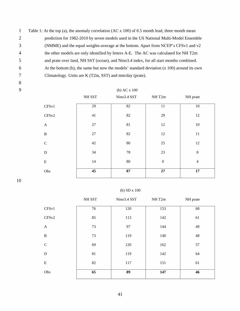
The top entry (a) of Table 1 shows the anomaly correlation for ½ month lead seasonal 6

prediction for SST, T2m and prate. These are aggregate numbers for all start months and large 7

areas combined. For SST (whether it is NH SST or Nino3.4) CFSv2 performs well, but so do 8

several or all of the other models, and the equal weight NMME (shown at the bottom row of the 9

Table 1a) is the best of all. The same applies for prate, but we note that the skill for prate over 10

NH land is extremely low for all the models. However, for NH T2m over land, CFSv2 is the best 11

model to such a degree that the NMME average of all models drags down the score of CFSv2. 12

The bottom entry (b) of Table 1 shows the interannual standard deviation of individual 13

members around the model climatology, all start months combined. This distributional property 14

in a grandly aggregated sense, is at least as large as that observed for any model (bottom row), 15

and CFSv2 is no exception. Not long ago, models were deemed to be underdispersive, and that 16

was the main reason why the multi-model approach would improve scores, especially 17

probabilistic scores. But, for the 3 month mean variables shown here, this is no longer true. 18

The distributional parameters being roughly correct in a grand sense does not preclude 19

standard deviations being too small, or too large, in specific areas and specific seasons, as we 20

saw already in section 4b. Additional insights can be gained from verification of probabilistic 21

verification in the next section. 22

4d. Probabilistic seasonal prediction verification 23

17

This section follows the CFSv1 paper (section 4b, pages 3495-3501) in S06 quite 1

precisely, both in terms of the definition of „reliability‟ and the Brier Skill Score (BSS) and the 2

corresponding figures (17 and 18 in S06) that will be shown. The difference is an additional six 3

years for CFSv1, and an exact comparison between CFSv1 and CFSv2 over the period 1982-4

2009, all start months, for a probabilistic prediction of the terciles of monthly Nino3.4 SST. 5

Figure 5 shows the reliability comparison, which is a make or break selling point for 6

probabilistic prediction. Plotted are observed frequency against predicted probability in 4 bins, 7

for each of the three terciles. Compared to perfection (the black line at 45 degrees), we see a 8

clear model improvement from CFSv1 to CFSv2. Keep in mind that CFSv2 was reduced to 15 9

members only (more are available) to be on an equal footing with CFSv1 in this display, as far as 10

the number of ensemble members is concerned. With 15 members each, CFSv2 has better 11

reliability than CFSv1. One can see this especially at lead 8, and for the notoriously difficult 12

„near normal‟ tercile. Using more ensemble members (not shown) further improves reliability, so 13

CFSv2 is a large improvement over CFSv1 in reliability, even though some problems were noted 14

in section 4b. 15

Figure 6 shows a comparison of the BSS, CFSv1 (v2) on the left (right). The BSS (full 16

line) has been decomposed in the usual contributions to BBS by reliability (dash dot) and 17

resolution (dotted). We do not show the third component called uncertainty since, by definition, 18

this is the same for both systems. Keep in mind that reliability (shown in another way in Fig.5) 19

has to be numerically small and resolution numerically high for a well calibrated system (i.e. to 20

contribute to a high BSS). Comparison of the left and right diagrams in Fig.6 indicates CFSv2 to 21

be an improvement over CFSv1, especially for longer leads and the near normal tercile. In terms 22

18

of their contribution to the total BSS, both resolution and reliability have helped to make CFSv2 1

better. 2

We did calculate the BSS for T2m over the United States (presented as a map in Figure 3

7), but neither CFSv1 nor CFSv2 has positive BSS overall for this domain, unless a very 4

laborious calibration is carried out. When only the mean and the standard deviation are corrected 5

and both systems are allowed 15 members (the maximum for CFSv1), the BSS scores for CFSv1 6

are slightly negative while those for CFSv2 are also negative, but closer to zero. It is only when 7

all 24 member are used that CFSv2 has positive BSS scores overall, see bottom row. The skill is 8

very modest nevertheless, with values such as +0.02 compared to 0.4-0.5 for Nino3.4 SST in 9

Figure 6. More aggressive suppression of noise and more calibration may improve the outcome 10

further, but this is outside the scope of this paper. In spite of many (modest) improvements in 11

these global models, we continue with the same basic discrepancy of having high skill for SST in 12

the tropics, but small and often negligible skill for T2m and especially Prate over land. 13

5. Diagnostics 14

While section 4 contains results of CFSv2 (vs. CFSv1) in terms of forecast skill, we also 15

need to report on some diagnostics that describe model behavior. Even without strict verification, 16

one may judge models as being „reasonable‟ or not. In section 5a we compare the systematic 17

errors globally in SST, T2m and prate between CFSv2 and CFSv1. Next the surface water 18

budget, which was mentioned in section 2 as being the subject of tuning, is discussed in section 19

5b. We also present some results on sea-ice prediction (without a strict verification) since this is 20

an important emerging aspect of global coupled models. CFSv1 had an interactive ocean only up 21

to 650 North and 75

0 South latitudes, with climatological sea-ice in the polar areas. The aspect of 22

19

a global ocean and interactive sea-ice model in the CFSv2 is new in the seasonal modeling 1

context at NCEP. 2

5a. Evolution of systematic error 3

The systematic error is defined as the difference in the predicted and observed 4

climatology over a common period, 1982-2009. We describe the systematic error here under the 5

header „model diagnostics‟ because it describes one of the net effects of modeling errors. While 6

the systematic error has a bearing on the forecast verification in section 4, its impact on the 7

verification was largely removed since we made hindcasts to apply the correction. Figure 8 8

shows global maps of the annual mean systematic error for the variables, from top to bottom, 9

T2m, prate and SST. On the left CFSv1 and on the right CFSv2, so this is the evolution of the 10

systematic error in an NCEP model from about 2003 to about 2010. The headers display 11

numbers for the mean and the root-mean-square (rms) difference averaged over the map. For all 12

three parameters CFSv2 has lower rms values, which is a definite sign of a better model. Lower 13

rms values globally does not preclude some areas having a larger systematic error, for instance 14

the cold bias over the eastern United States is stronger in CFSv2. Figure 8 is for a lead of 3 15

months, but these maps looks very similar for all leads from 1 to 8 months. Apparently these 16

models settle quickly in their respective climatological distributions. The systematic error has a 17

sign, so the map mean shows a cold bias (-0.3K) and a wet bias (+0.6-0.7mm/day) globally 18

averaged in both models. Of these three maps the one for T2m has changed the least between the 19

CFSv1 and CFSv2 versions, the maps for prate have changed some more, especially in the 20

tropics, but note that the SST systematic error has changed beyond recognition from v1 to v2. 21

Another „evolution‟ of the systematic error is displayed in Figure 9 where we compare, 22

just for CFSv2, the systematic error as calculated for 1982-1998 (left) and 1999-2009 (right). In 23

20

a constant frozen system the maps on the left and right should be the same, except for sampling 1

error. From a global standpoint these maps are quite similar, but if one focusses on the tropical 2

Pacific we should point out a difference in the SST maps right in the Nino34 area. The later 3

years (past 1998) have a negligible systematic error, while the earlier years have a modest cold 4

bias. Perhaps this makes perfect sense because in later years the models are initialized with much 5

more data. On the other hand it is a problem in systematic error correction, if the systematic error 6

is non-stationary (Kumar et al., 2012). 7

The SST in the Nino3.4 area is important as this area is often chosen as the most sensitive 8

single indicator of ENSO. And one may surmise that changes in the systematic error in prate are 9

caused by the model predicted SST being warmer in later years. Indeed, one can see large 10

changes in the Pacific basin in the ITCZ in the NH, the SPCZ in the SH, and the rainfall in the 11

western Pacific, see middle row in Figure 9. The rest of the globe is not impacted so obviously in 12

terms of either SST or prate, not even the Atlantic and Indian tropical Oceans. The systematic 13

error in T2m over land appears oblivious to changes in SST in the Pacific. 14

The causes of this discontinuity are most probably related to ingest of new data systems, 15

most notably AMSU in late 1998 (Saha et al., 2010, p1041, p1044), which caused an enormous 16

increase in satellite data to be assimilated. Such issues need to be addressed in CFSv3, and 17

specifically in any Reanalyses that are made in the future to create initial conditions (land, ocean 18

and atmosphere) for CFSv3 or systems elsewhere. But, for the time being, we need to address 19

how we apply the systematic error correction in the CFSv2 hindcasts, and in real time 20

(subsequent) CFSv2 forecasts. Our recommendation is that the full 30 year period (1982-2012 is 21

now available for CFSv2) be used for all fields globally with the exception of SST and prate in 22

the Pacific Ocean basin where it seems better to use a split climatology. Therefore for real time 23

21

forecasts, the systematic error correction for prate and SST in the Pacific should be based on 1

1999-present. This does not mean that anomalies should be presented as departures from the 2

1999-present climatology, see ZV for that distinction. 3

5b. Land Surface 4

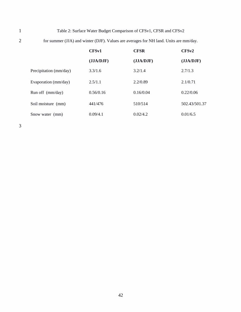
Table 2 shows a comparison of surface water budget terms averaged over the Northern 5

Hemisphere land between CFSv1 and CFSv2 and with CFSR. The quantities in CFSv1 and 6

CFSv2 are computed from seasonal ensemble means covering a 29-yr period (1982-2010), where 7

the CFSv1 is based on seasonal predictions from 15 ensemble members whose initial conditions 8

are from Mid-April to early May (April 9-13, 19-23, and April 29-May 3 at 00Z) for the summer 9

season (JJA), and from Mid-October to early November (October 9-13, 19-23, and October 29 –10

November 3) for the winter season (DJF), while the CFSv2 is based on 24 ensemble members ( 11

initial conditions from 4 cycles of the 6 days between April 11 and May 6 with 5 days apart) for 12

summer and 28 ensemble members (initial conditions from 4 cycles of 7 days between October 8 13

and November 7 with 5 days apart) for winter season, respectively. 14

Compared to the CFSR, precipitation (snow in winter) in the CFSv1 is higher in both 15

seasons, which yields higher values for both evaporation and runoff. The higher evaporation in 16

the summer season in the CFSv1 yields a much larger seasonal variation in soil moisture (though 17

lower absolute values) than in both CFSR and CFSv2. In contrast, precipitation in the CFSv2 is 18

considerably lower than in both CFSv1 and CFSR, consistent with lower evaporation in the 19

CFSv2. While less than the CFSv1, runoff in the CFSv2 is more than in CFSR, indicating that 20

soil moisture is a more important source for surface evaporation in the CFSv2; this higher runoff 21

in winter season leads to a damped seasonal variation in soil moisture since soil moisture is re-22

charged in winter when evaporation is at its minimum. The increases in both surface evaporation 23

from root-zone soil water and runoff production are consistent with the changes made to 24

22

vegetation parameters and rooting depths in CFSv2 ( see comments in section 2) to address high 1

biases in predicted T2m, and the accommodated changes in soil moisture climatology and 2

surface runoff parameters. The good agreement in soil moisture between CFSR and CFSv2 is 3

expected because they use the same Noah land model. 4

5c. Sea Ice 5

Sea ice prediction is challenging and relatively new in the context of seasonal climate 6

prediction models. Sea ice can form or melt and can move with wind and/or ocean current. Sea 7

ice interacts with both the air above and the ocean beneath and it is influenced by, and has 8

impact on, the air and ocean conditions. The CFSv2 sea ice component includes a 9

dynamic/thermodynamic sea ice model and a simple "assimilation" scheme, which are described 10

in details in Saha et al. (2010). One of the most important developments in CFSv2, compared to 11

CFSv1, is the extension of the CFS ocean domain to the global high latitudes and the 12

incorporation of a sea ice component. 13

The ice initial condition (IC) for the CFSv2 hindcasts is from CFSR as described in Saha et al. 14

(2010). For sea ice thickness, there is no data available for assimilation, and we suspect there is a 15

significant bias of sea ice thickness in the CFSv2 model, which causes the sea ice to be too thick 16

in the IC. For the sea ice prediction, sea ice appears too thick and certainly too extensive in the 17

spring and summer. Figure 10 shows the mean September sea ice concentration from 1982 to 18

2010, and the bias in the predicted mean condition at lead times of 1-month (August 15 IC), 3-19

month (June 15 IC), and 6-month (March 15 IC). The model shows a consistent high bias in its 20

forecasts of September ice extent. The corresponding predicted model variability at the 3 21

different lead times is shown in Figure 11. The variability from the model prediction is 22

underestimated near the mean September ice pack and overestimated outside the observed mean 23

23

September ice pack. Although the CFSv2 captured the observed seasonal cycle, long-term trend 1

and interannual variability to some extent, large errors exist in its representation of the observed 2

mean state and anomalies, as shown in Figures 9 and 10. Therefore in the CFSv2, when the sea 3

ice predictions are used for practical applications, bias correction is necessary. The bias can be 4

obtained from the hindcast data for the period 1982-2010, which are available from NCDC. 5

In spite of the above reported shortcomings, when the model was used for the prediction of the 6

September minimum sea ice extent organized by SEARCH (Study of Environmental Arctic 7

Change) during 2009 and 2011, CFSv2 (with bias correction applied) was among the best 8

prediction models. In the future we plan to assimilate the sea ice thickness data into the CFS 9

assuming that would reduce the bias and improve the sea ice prediction. 10

6. Model behavior in very long integrations. 11

6a. Decadal prediction 12

The protocol for the 2014 IPCC (Inter Governmental Panel for Climate Change) model 13

runs, called AR5, recommended the making of decadal predictions to assist in the study of 14

climate change, see: http://www.ipcc.ch/activities/activities.shtml#.UGyOHpH4Jw0 15

These decadal runs may bring in elements of the initial states in terms of land, ocean, sea ice and 16

atmosphere and thus perhaps add information in the first 10 years, in addition to the general 17

warming that most models may predict when greenhouse gases (GHG) increase. Following this 18

recommendation, sixty 10-year runs were made from initial conditions on Nov 1, 0Z, 6Z, 12Z 19

and 18Z cycles (i.e. 4 „members‟), for the following years: 1980, 1981, 1983, 1985, 1990, 1993, 20

1995, 1996, 1998, 2000, 2003, 2005, 2006, 2009 and 2010 (every 5th

year from 1980 to 2010, as 21

well as some interesting intermediate years). Each run was 122 months long (the first 2 months 22

were not used to avoid spin-up). The forcing for these decadal runs included both shortwave and 23

24

longwave tropospheric aerosol effects and is from a monthly climatology that repeats its values 1

year after year (described in Hou et al, 2002). Also, included in the runs are historical 2

stratospheric volcanic aerosol effects on both shortwave and longwave radiation, which end in 3

1999, after which a minimum value of optical depth=1e-4 was used (Sato et al, 1993). The runs 4

also used the latest observed CO2 data when available (WMO Global Atmospheric Watch 5

(http://gaw.kishou.go.jp) and an extrapolation was done into the future with a fixed growth rate 6

of 2ppmv. 7

Results using only monthly mean data from the 60 decadal runs are presented in this 8

paper. Variable X in an individual run can be denoted as X j, m, where j and m is the target year 9

and month. How „anomalies‟ are obtained is not obvious in these type of decadal runs. We 10

proceeded as follows: first a 60 run mean was formed, i.e. <X j, m>, where j=1, 10 and m=1, 120. 11

Averaging across all years, we get <<X m>>. The anomaly is then computed as X j, m - <<Xm>>. 12

Figure 12a (top panel) shows the global mean SST anomalies (here X is SST). There are 60 13

yellow traces, each of 10 year length. The observations (Reynolds et al, 2007) are shown as the 14

full black line, and the monthly anomaly is formed as the departure from 1982-2010 climatology. 15

One can conclude that the observations are in the cloud of model traces produced by CFSv2, 16

especially after 1995 and before 1987 when the observations are near the middle of the cloud. 17

The model appears somewhat cold in the late eighties and early nineties. Figure 12b (bottom 18

panel) shows the same thing, but for global mean land temperature. The black line, from GHCN-19

CAMS (Fan and Van den Dool, 2008, which is a combinations of the Global Historical Climate 20

Network with the observation in CPC‟s Climate Anomaly Monitoring System)), is comfortably 21

inside the cloud of model traces, except around 1993 when perhaps the model overdid the 22

aerosol impact of the Pinatubo volcanic eruption. The spread produced by the model is much 23

25

higher in Figure 12b than in Figure 12a, not only because the land area is smaller than the 1

oceanic area, but also because the air temperature is much more variable to start with. This 2

model, never before exposed to such long integrations, passed the zeroth

order test, in that it 3

produced some warming over the period from 1980 to the present and has enough spread to 4

cover what was observed (essentially a single model trace). In this paper there is no attempt to 5

address any model prediction skill over and beyond a capability to show general warming and 6

uncertainty. 7

Some monthly mean and 3-hourly time series data from the NCEP decadal runs is available for 8

download (see Appendix D) 9

6b. Long ‘free’ runs 10

On the very long time-scales, a few single runs were made lasting from 43 to 100 years, 11

which were designated as „CMIP‟ runs. There is nothing that reminds these runs of the calendar 12

years they are in, except for GHG levels which are prescribed when available (see section 4c), 13

and in case of CO2 is projected to increase by 2ppm in future years. Here, we are interested in 14

behavioral aspects, including a test as to whether the system is even stable or drifting due to 15

assorted technical issues. The initial conditions were chosen for Jan of three years, namely 1987, 16

1995, and 2001 (similar runs were made with the first version of the CFS). Allowing for a spin 17

up of 1 year, data was saved for 1988-2030 (43 years), 1996-2047 (52 years) and 2002-2101 18

(100 years) from these three runs, one of which is truly centennial. None of these runs became 19

unstable or produced completely unreasonable results. A common undesirable feature (not a real 20

forecast!) was a slow cooling of the upper ocean for the first 15-20 years. Only after this 21

temperature decline stabilized, a global warming of the sea surface temperature was seen starting 22

26

25-35 years after initial time. In contrast, the water at the bottom of the ocean showed a small 1

warming from the beginning to end, which is unlikely to be correct. 2

An important issue was to examine the onset and decay of warm and cold events (El Ninos and 3

La Ninas) and ascertain how regular they were. The CFSv1 was found to be too regular and very 4

close to being periodic in its CMIP runs (Penland and Saha, 2006) when diagnosed via a spectral 5

analysis of Nino3.4 monthly values. Figure 13 shows the spectra of Nino3.4 for the observations 6

from 1950-2011 (upper left) and the three CFSv2 CMIP runs. A harmonic analysis was 7

conducted on monthly mean data with a monthly climatology removed. Raw power was 8

estimated as ½ of the amplitude (of the harmonic) squared. The curves shown were smoothed by 9

a 1-2-1 filter. The variance of all the CMIP runs is higher than observed by at least 25%, 10

therefore the integral under the blue (model) and black (observed) curves differs. The model 11

variance being too large was already noted in Figure 3 for leads of 3 and 6 months, and in Table 12

1 for many other fields and areas. The observations have a broad spectral maximum from 0.15 to 13

0.45 cycles per year (cpy). The shortest of the CMIP runs (upper right) resembles the broad 14

spectral maximum quite well, the longer runs are somewhat more sharply peaked but are not 15

nearly as periodic as in CMIP runs made by CFSv1, especially when T62 resolution was used 16

(Penland and Saha 2006). On the whole, the behavioral aspects of ENSO (well beyond 17

prediction) appear acceptable. One may also consider the possibility that certain segments of 43 18

years from the 100 year run may look like the upper right entry. Or by the same token, that the 19

behavior of observations for 1951-2011 are not necessarily reproduced exactly when a longer 20

period could be considered, or a period without mega-events like the 1982/83 and 1997/98 21

ENSO events. Some data from these CMIP runs are available for download from the CFS 22

website (see Appendix D). 23

27

7. Concluding Remarks 1

This paper describes the transition from the CFSv1 to the CFSv2 operational systems. 2

The Climate Forecast System (CFS), retroactively named version 1, was operationally 3

implemented at NCEP in August 2004. The CFSv1 was described in S06. Its successor, named 4

CFSv2, was implemented in March 2011 even though version 1 was only decommissioned in 5

October 2012. The overlap (1.5 years) was needed, among other things, to give users time to 6

make their transition between the two systems. In contrast to most implementations at NCEP, the 7

CFS is accompanied by a set of retrospective forecasts that can be applied by the user 8

community to calibrate subsequent real time operational forecasts made by the same system. 9

Therefore, a new CFS takes time to develop and implement both on the part of NCEP and on the 10

side of the user. One element that took a lot of time at NCEP to complete, was a new Reanalysis 11

(the CFSR), that was needed to create the initial conditions for the coupled land-atmosphere-12

ocean-seaice CFSv2 retrospective forecasts. Every effort was made to create these initial 13

conditions (for the period 1979-present) with a forecast system that was as consistent as possible 14

with the model used to make the long range forecasts, whether it be for the retrospective 15

forecasts or the operational forecasts going forward in real time. 16

For convenience, the evolution of the model components between CFSv1 and CFSv2 has been 17

split into two portions, namely the very large model developments between CFSv1 and CFSR, 18

and the far smaller model developments between CFSR and CFSv2. The development of model 19

components between the time of CFSv1 (of 1996-2003 vintage) and CFSR (of 2008-2010 20

vintage) to generate the background guess in the data assimilation has already been documented 21

in Saha et al (2010). Therefore, in the present paper, we only describe some further 22

28

adjustments/tunings of the land surface parameters and clouds in the equatorial SST (in section 1

2). 2

The paper describes the design of both the long lead seasonal (out to 9 months) and shorter lead 3

intraseasonal predictions (out to 45 days) for the retrospective forecasts and the real-time 4

operational predictions going forward. This information is essential for any user who may want 5

to use these forecasts. The retrospective forecasts are important for both calibration and skill 6

estimates of subsequent real time prediction. The size of the hindcast data set is very large, since 7

it spans forecasts from 1982-present for long lead seasonal range (4 runs out to 9 month, every 8

5th

day), and forecasts from 1999-present for intraseasonal range (3 runs each day out to 45 days, 9

plus one run each day out to 90 days), with all model forecast output data archived at 6 hour 10

intervals for each run. 11

The paper also describes some of the results, in terms of the forecast skill, determined from the 12

retrospective forecasts, for the prediction of the intraseasonal component (MJO in particular), 13

and the seasonal prediction component (in section 4). This is done by comparing, very precisely, 14

the CFSv2 predictions to exactly-matching CFSv1 predictions. There is no doubt that CFSv2 is 15

superior to CFSv1 on the intraseasonal time scale; in fact the improvement is impressive from 1 16

week to more than 2 weeks (at the 0.5 level of anomaly correlation) for MJO prediction. For 17

seasonal prediction, we note a substantial improvement in 2 meter temperature prediction over 18

global land. This is mainly a result of successfully simulating temperature trends (which are 19

large over the 1980-2010 period and thus an integral part of any verification) by increasing the 20

amount of prescribed greenhouse gases in the model (a feature that was missing in CFSv1). For 21

precipitation over land, the CFSv2, unfortunately, is hardly an improvement over CFSv1. This is 22

perhaps due to the predictability ceiling being too low to expect big leaps forward in prediction. 23

29

The SST prediction has been improved modestly over most of the global oceans and extended in 1

CFSv2 to areas where CFSv1 had prescribed SST and/or sea-ice, as well as over the extra-2

tropical oceans. In the tropics, SST prediction has also improved, but least so in the much-3

focused-on Nino3.4 area, where the subsurface initial states of CFSR show warming after 1998, 4

due to the introduction of the AMSU satellite data. Before that time, the SST forecasts were too 5

cold in that area, thus making the systematic error correction a challenge. 6

Being a community model to some extent, the CFSv2 has been (and will be) applied to decadal 7

and centennial runs. These have not been typical NCEP endeavors in the past, so we have tested 8

the behavior of this new model in integrations beyond the operational 9-month runs. Some 9

results are described in section 6. The decadal runs appear reasonable in that, in the global mean, 10

reality is within the cloud of the 65 decadal runs, both for 2 meter temperature over land and for 11

SST in the ocean. The three centennial runs did not de-rail (a minimal test passed), and show 12

both reasonable and unreasonable behavior. Unreasonable, we believe, is a small but steady 13

cooling of the global ocean surface that lasts about 15 years before GHG forced warming sets in. 14

Equally unreasonable may be a small warming of the bottom layers of global oceans from start to 15

finish. The better news is that the ENSO spectrum in these free runs is far more acceptable in 16

CFSv2, in contrast to CFSv1. When run in its standard resolution of T62L64, the CFSv1 17

produced too regular and almost periodic ENSO in its free runs, lasting up to a century. 18

A few diagnostics (presented in section 5) were made in support of the need for tuning some of 19

the land surface parameters when going from CFSR to CFSv2. The main concern was the fact 20

that the NH mean precipitation in summer over land reduced from 3.2 mm/day in CFSR to 2.7 21

mm/day in CFSv2 which posed a real problem for improved prediction of evaporation, runoff 22

and surface air temperature. Some diagnostics are also presented for the emerging area of 23

30

coupled sea-ice modeling, imbedded in a global ocean. Although this topic is important for 1

monthly seasonal prediction, it has taken on new urgency due to concerns over shrinking sea-ice 2

coverage (and thickness) in the Arctic. It is easy to identify some large errors in sea-ice coverage 3

and variability and it is obvious that a lot more work needs to be done in this area of seaice 4

modeling. 5

This paper is mainly to describe CFSv2 as a whole, from inception to implementation. There are 6

many subsequent papers in preparation (or submitted/published) about detailed studies of CFSv2 7

prediction skill and/or diagnostics of some of the parts of CFSv2, whether it be the stratosphere, 8

troposphere, deep oceans, land surface, etc. 9

While there are many users for the CFS output (sometimes one finds out how many only by 10

trying to discontinue a model), the first line user is the Climate Prediction Center at NCEP. The 11

CFSv2 plays a substantial role in the seasonal prediction efforts at CPC, both directly and 12

through joint efforts such as National and International Multi-Model Ensembles.2 CFSv2 is also 13

used in the sub seasonal MJO prediction, and in a product called international hazards 14

assessment. Because CFSv2 runs practically in real time (compared to CFSv1 which was about 15

36 hours later than real time), it plays a role in the operational 6-10day and week 2 forecasts and 16

conceivably in the future prediction of the week 3 – week 6 forecasts for the US, which is on the 17

drawing board at CPC. The appropriate forcing fields extracted from CFSv2 predictions, such as 18

daily radiation, precipitation, wind, relative humidity, etc. are used to carry the Global Land Data 19

Assimilation Systems (GLDAS) forward, yielding an ensemble of drought related indices over 20

the US and soon globally. 21

22

2 We should point out that what we call the International Multi-Model Ensembles (IMME) has its counterpart called Eurosip in Europe. CFSv2

has been admitted as a member in the Eurosip ensemble which consists of the ECMWF, UK Met Office and Meteo France.

31

Acknowledgements 1

The authors would like to recognize all the scientists and technical staff of the Global 2

Climate and Weather Modeling Branch of EMC for their hard work and dedication to the 3

development of the GFS. We would also like to extend our thanks to the scientists at GFDL for 4

their work in developing the MOM4 Ocean model. George Vandenberghe, Carolyn Pasti and 5

Julia Zhu are recognized for their critical support in the smooth running of the CFSv2 6

retrospective forecasts and the operational implementation of the CFSv2. We also thank Ben 7

Kyger, Dan Starosta, Christine Magee and Becky Cosgrove from the NCEP Central Operations 8

(NCO) for the timely operational implementation of the CFSv2 in March 2011. 9

32

Appendix A: Reforecast Configuration of the CFSv2 (Figure A1) 1

• 9-month hindcasts were initiated from every 5th

day and run from all 4 cycles of that day, 2

beginning from Jan 1 of each year, over the full 29 year period from 1982-2010. This is 3

required to calibrate the operational CPC longer-term seasonal predictions (ENSO, etc) 4

(full lines in Figure A1). 5

• There was also a single 1 season (123-day) hindcast run, initiated from every 0 UTC 6

cycle between these five days, but only over the 12 year period from 1999-2010. This is 7

required to calibrate the operational CPC first season predictions for hydrological 8

forecasts (precip, evaporation, runoff, streamflow, etc) (dashed lines in Figure A1) 9

• In addition, there were three 45-day hindcast runs from every 6, 12 and 18 UTC cycles, 10

over the 12-year period from 1999-2010. This is required for the operational CPC week3-11

week6 predictions of tropical circulations (MJO, PNA, etc) (dotted lines in Figure A1) 12

• Total number of years of integration = 9447 years. 13

33

APPENDIX B: Retrospective Forecast Calendar (292 runs per year) 1

Organized by date of release of the official CPC seasonal prediction every month 2

As outlined in Appendix A, four 9-month retrospective forecasts are made every 5th

day 3

over the period 1982-2010. The calendar always starts on January 1 and proceeds forward 4

in the same manner each year. Forecasts are always made from the same initial dates 5

every year. This means that in leap years, Feb 25 and March 2 are separated by 6 days 6

(instead of 5). Table A1 describes the grouping of the retrospective forecasts in relation 7

to CPC‟s operational schedule (all forecast products must be available a week before the 8

official release on the third Thursday of each month). For instance, for the release of the 9

official forecast in the month of February, all retrospective forecasts made from initial 10

conditions over the period from 11th

January through Feb 5th

for all previous years can be 11

used for calibration and skill estimates, which constitute a lagged ensemble of 24 12

members. Obviously one can use more (going back farther), or less (since older forecasts 13

may have much less skill). 14

All real time forecasts that are available closest to the date of release are used (see 15

Appendix C). 16

34

Appendix C: Operational Configuration of the CFSv2 for a 24-hour period (Figure A2) 1

• There are 4 control runs per day from the 0, 6, 12 and 18 UTC cycles of the CFSv2 real-2

time data assimilation system, out to 9 months (full lines in Fig A2) 3

• In addition to the control run of 9 months, there are 3 additional runs at 0 UTC out to one 4

season. These 3 perturbed runs are initialized as in current operations (dashed lines in 5

Figure A2) 6

• In addition to the control run of 9 months at the 6, 12 and 18 UTC cycles, there are 3 7

additional perturbed runs, out to 45 days. These 3 runs per cycle are initialized as in 8

current operations (dotted lines in Figure A2) 9

• There are a total of 16 CFS runs every day, of which four runs go out to 9 months, three 10

runs go out to 1 season and nine runs go out to 45 days. 11

35

APPENDIX D: Availability of CFSv2 data 1

Real time operational data: Users must maintain their own continuing archive by 2

downloading the real time operational data from the 7-day rotating archive located at: 3

http://nomads.ncep.noaa.gov/pub/data/nccf/com/cfs/prod/ 4

This site includes both the initial conditions and forecasts made at each cycle of each day. 5

Monthly means of the initial conditions are posted once a month and can be downloaded 6

from a 6-month rotating archive at the same location given above. 7

Selected data from the CFSv2 retrospective forecasts (both seasonal and sub seasonal) for the 8

forecast period 1982-2010, may be downloaded from the NCDC web servers at: 9

(http://nomads.ncdc.noaa.gov/data.php?name=access#cfs) 10

Smoothed calibration climatologies have been prepared from the forecast monthly means and 11

time series of selected variables and is available for download from the CFS website 12

(http://cfs.ncep.noaa.gov). Please note that two sets of climatologies have been prepared for 13

calibration, for the full period (1982-2010) and the later period (1999-2010). We highly 14

recommend that the climatology prepared from the later period be used when calibrating real 15

time operational predictions for variables in the tropics, such as SST and precipitation over 16

oceans. For skill estimates, we recommend that split climatologies be used for the two 17

periods when removing the forecast bias. 18

A small amount of CFSv2 forecast data for 2011-present may be found at the CFS website at 19

http://cfs.ncep.noaa.gov/cfsv2/downloads.html 20

Decadal runs : Some monthly mean and 3-hourly time series data from the NCEP decadal 21

runs may be obtained from the ESGF/PMDI website at 22

http://esgf.nccs.nasa.gov/esgf-web-fe/ 23

36

CMIP runs : Monthly mean data from the 3 CMIP runs is available for download from the 1

CFS website at: http://cfs.ncep.noaa.gov/pub/raid0/cfsv2/cmipruns 2

37

References 1

Barker, H. W., R. Pincus, and J-J. Morcrette, 2002: The Monte Carlo Independent Column 2

Approximation: Application within large-scale models. Extended Abstracts, GCSS-ARM 3

Workshop on the Representation of Cloud Systems in Large-Scale Models, Kananaskis, 4

AB, Canada, GEWEX, 1–10. [Available online at 5

http://www.met.utah.edu/skrueger/gcss-2002/Extended-Abstracts.pdf.]. 6

Cai, Ming, Chul-Su Shin, H. M. van den Dool, Wanqiu Wang, S. Saha, A. Kumar, 2009: The 7

Role of Long-Term Trends in Seasonal Predictions: Implication of Global Warming in 8

the NCEP CFS. Wea. Forecasting, 24, 965–973. doi: 10.1175/2009WAF2222231.1 9

Chun, H.-Y, and J.-J. Baik, 1998: Momentum Flux by Thermally Induced Internal Gravity Wave 10

and its Approximation for Large-Scale Models. Journal of the Atmospheric Sciences, 55, 11

3299-3310. 12

Clough, S.A., M.W. Shephard, E.J. Mlawer, J.S. Delamere, M.J. Iacono, K. Cady-Pereira, 13

S. Boukabara, and P.D. Brown, 2005: Atmospheric radiative transfer modeling: a 14

summary of the AER codes, J. Quant., Spectrosc. Radiat. Transfer, 91, 233-244. 15

Behringer, D. W. 2007. The Global Ocean Data Assimilation System at NCEP. 11th Symposium on 16

Integrated Observing and Assimilation Systems for Atmosphere, Oceans and Land Surface, 17

AMS 87th Annual Meeting, San Antonio, Texas, 12pp 18

Ek, M., K. E. Mitchell, Y. Lin, E. Rogers, P. Grunmann, V. Koren, G. Gayno, and J. D. Tarpley, 19

2003: Implementation of Noah land-surface model advances in the NCEP operational 20

mesoscale Eta model. J. Geophys. Res., 108(D22), 8851, doi:10.1029/ 2002JD003296. 21

38

Fan, Y., and H. van den Dool (2008), A global monthly land surface air temperature analysis for 1

1948––present, J. Geophys. Res., 113, D01103, doi:10.1029/2007JD008470. 2

Hou, Y., S. Moorthi and K. Campana, 2002: Parameterization of Solar Radiation Transfer in the 3

NCEP Models. NCEP Office Note 441. 4

http://www.emc.ncep.noaa.gov/officenotes/newernotes/on441.pdf 5

Iacono, M.J., E.J. Mlawer, S.A. Clough, and J.-J. Morcrette, 2000: Impact of an improved 6

longwave radiation model, RRTM, on the energy budget and thermodynamic 7

properties of the NCAR Community Climate Model, CCM3, J. Geophys. Res., 8

105, 14873-14890, 2000. 9

Kanamitsu, M., W. Ebisuzaki, J. Woollen, S.K. Yang, J.J. Hnilo, M. Fiorino, and G.L.Potter, 10

2002: NCEP–DOE AMIP-II Reanalysis (R-2). Bull. Amer. Meteor. Soc., 83, 1631–1643. 11

Kirtman, B. P., D. Min, J.M. Infanti, J.L. Kinter III, D. A. Paolino, Q. Zhang, 12

H. van den Dool, S. Saha, M. Peña Mendez, E. Becker, P. Peng, P. Tripp, J. Huang, 13

D. G. DeWitt, M. K. Tippett, A. G. Barnston, S. Li, A. Rosati, S. D. Schubert, Y-K. Lim, 14

Z. E. Li, J. Tribbia, K. Pegion, W. Merryfield, B. Denis and E. Wood, 2012: The US 15

National Multi-Model Ensemble for Intra-Seasonal to Interannual Prediction. Bull. Amer. 16

Meteor. Soc. In review. 17

Kumar, A., M. Chen, L. Zhang, W. Wang, Y. Xue, C. Wen, L. Marx, B. Huang, 2012: An Analysis 18

of the Nonstationarity in the Bias of Sea Surface Temperature Forecasts for the NCEP 19

Climate Forecast System (CFS) Version 2. Mon. Wea. Rev., 140, 3003–3016. 20

39

doi: http://dx.doi.org/10.1175/MWR-D-11-00335.1 1

Lin, H., G. Brunet, and J. Derome (2008), Forecast skill of the Madden–Julian oscillation in two 2

Canadian atmospheric models. Mon. Wea. Rev., 136, 4130–4149. 3

Mitchell, K. E., H. Wei, S. Lu, G. Gayno and J. Meng, 2005: NCEP implements major upgrade to 4

its medium-range global forecast system, including land-surface component. GEWEX 5

newsletter, May 2005. 6

Mlawer E. J., S. J. Taubman, P. D. Brown, M.J. Iacono and S.A. Clough, 1997: radiative 7

transfer for inhomogeneous atmosphere: RRTM, a validated correlated-K model 8

for the longwave. J. Geophys. Res., 102(D14), 16,663-16,6832. 9

Moorthi, S., R. Sun, H. Xia, and C. R. Mechoso, 2010: Low-cloud simulation in the 10

Southeast Pacific in the NCEP GFS: role of vertical mixing and shallow 11

convection. NCEP Office Note 463, 28 pp [Available online at 12

http://www.emc.ncep.noaa.gov/officenotes/FullTOC.html#2000 ] 13

Pincus, R., H.W. Barker, and J.-J. Morcrette, 2003: A fast, flexible, approximate technique for 14

computing radiative transfer in inhomogeneous cloud fields. J. Geophys. Res., 108(D13), 15

4376, doi:10.1029/2002JD003322. 16

Penland and Saha, 2006: El Nino in the Climate Forecast System: T62 vs T126. Poster 1.3 at 17

Climate Diagnostic and Prediction Workshop #30. Available online at 18

http://www.cpc.ncep.noaa.gov/products/outreach/proceedings/cdw30_proceedings/P1.3.pdf 19

Reynolds, R. W., N. A. Raynor, T. M. Smith, D. C. Stokes, and W. Wang, 2002: An improved in 20

situ and satellite SST analysis for climate. J. Climate, 15, 1609-1625. 21

Reynolds, R. W., T. M. Smith, C. Liu, D. B. Chelton, K. S. Casey, and M. G. Schlax, 2007: Daily 22

40

high-resolution blended analyses for sea surface temperature. J. Climate, 20, 5473–5496. 1

Saha, S. and Coauthors, 2006: The NCEP climate forecast system, J. Climate, 19, 3483-3517. 2

Saha, S. and Coauthors, 2010: The NCEP climate forecast system reanalysis. Bull. 3

Amer. Meteor. Soc., 91, 1015-1057. 4

Sato, M., Hansen, J.E., McCormick, M.P., and Pollack, J.B., 1993, Stratospheric aerosol optical 5

depths, 1850-1990: J. Geophys. Res., 98, 22987-22994. 6

Sun, R., S. Moorthi and C. R. Mechoso, 2010: Simulaton of low clouds in the Southeast Pacific 7

by the NCEP GFS: sensitivity to vertical mixing. Atmos. Chem. Phys., 10, 12261-12272. 8

Vitart, Frédéric, Steve Woolnough, M. A. Balmaseda, A. M. Tompkins, 2007: Monthly Forecast 9

of the Madden–Julian Oscillation Using a Coupled GCM. Mon. Wea. Rev., 135, 2700–10

2715. doi: http://dx.doi.org/10.1175/MWR3415.1 11

Wheeler, M, and H. H. Hendon (2004), An all-season real-time multivariate MJO index: 12

Development of an index for monitoring and prediction. Mon. Wea. Rev., 132, 1917–13

1932. 14

Zhang, Qin, Huug van den Dool, 2012: Relative Merit of Model Improvement versus 15

Availability of Retrospective Forecasts: The Case of Climate Forecast System MJO 16

Prediction. Wea. Forecasting, 27, 1045–1051. doi: http://dx.doi.org/10.1175/WAF-D-17

11-00133.1 18

41

Table 1: At the top (a), the anomaly correlation (AC x 100) of 0.5 month lead, three month mean 1

prediction for 1982-2010 by seven models used in the US National Multi-Model Ensemble 2

(NMME) and the equal weights-average at the bottom. Apart from NCEP‟s CFSv1 and v2 3

the other models are only identified by letters A-E. The AC was calculated for NH T2m 4

and prate over land, NH SST (ocean), and Nino3.4 index, for all start months combined. 5

At the bottom (b), the same but now the models‟ standard deviation (x 100) around its own 6

Climatology. Units are K (T2m, SST) and mm/day (prate). 7

8

(b) AC x 100 9

NH SST Nino3.4 SST NH T2m NH prate

CFSv1 29 82 11 10

CFSv2 41 82 29 12

A 27 81 12 10

B 27 82 12 11

C 42 80 25 12

D 34 78 23 8

E 14 80 0 4

Obs 45 87 27 17

10

(b) SD x 100

NH SST Nino3.4 SST NH T2m NH prate

CFSv1 76 120 153 68

CFSv2 85 113 142 61

A 73 97 144 49

B 73 119 140 48

C 69 120 162 57

D 81 119 142 64

E 82 117 151 61

Obs 65 89 147 46

42

Table 2: Surface Water Budget Comparison of CFSv1, CFSR and CFSv2 1

for summer (JJA) and winter (DJF). Values are averages for NH land. Units are mm/day. 2

CFSv1

(JJA/DJF)

CFSR

(JJA/DJF)

CFSv2

(JJA/DJF)

Precipitation (mm/day) 3.3/1.6 3.2/1.4 2.7/1.3

Evaporation (mm/day) 2.5/1.1 2.2/0.89 2.1/0.71

Run off (mm/day) 0.56/0.16 0.16/0.04 0.22/0.06

Soil moisture (mm) 441/476 510/514 502.43/501.37

Snow water (mm) 0.09/4.1 0.02/4.2 0.01/6.5

3

43

Table A1 CFSv2 Retrospective Calendar 1 (organized by date of release of the official CPC seasonal prediction every month) 2

3 MID JANUARY RELEASE (24 members) MID JULY RELEASE (24 members) 4 12 December at 0, 6 12 and 18 Z 10 June at 0, 6 12 and 18 Z 5 17 December at 0,6,12 and 18 Z 15 June at 0,6,12 and 18 Z 6 22 December at 0,6,12 and 18 Z 20 June at 0,6,12 and 18 Z 7 27 December at 0,6,12 and 18 Z 25 June at 0,6,12 and 18 Z 8 1 January at 0,6,12 and 18 Z 30 June at 0,6,12 and 18 Z 9 6 January at 0,6,12 and 18 Z 5 July at 0,6,12 and 18 Z 10 11 MID FEBRUARY RELEASE (24 members) MID AUGUST RELEASE (24 members) 12 11 January at 0, 6 12 and 18 Z 10 July at 0,6,12 and 18 Z 13 16 January at 0,6,12 and 18 Z 15 July at 0,6,12 and 18 Z 14 21 January at 0,6,12 and 18 Z 20 July at 0,6,12 and 18 Z 15 26 January at 0,6,12 and 18 Z 25 July at 0,6,12 and 18 Z 16 31 January at 0,6,12 and 18 Z 30 July at 0,6,12 and 18 Z 17 5 February at 0,6,12 and 18 Z 4 August at 0,6,12 and 18 Z 18 19 MID MARCH RELEASE (24 members) MID SEPTEMBER RELEASE (24 members) 20 10 February at 0, 6 12 and 18 Z 9 August at 0,6,12 and 18 Z 21 15 February at 0,6,12 and 18 Z 14 August at 0,6,12 and 18 Z 22 20 February r at 0,6,12 and 18 Z 19 August at 0,6,12 and 18 Z 23 25 February at 0,6,12 and 18 Z 24 August at 0,6,12 and 18 Z 24 2 March at 0,6,12 and 18 Z 29 August at 0,6,12 and 18 Z 25 7 March at 0,6,12 and 18 Z 3 September at 0,6,12 and 18 Z 26 27 MID APRIL RELEASE (24 members) MID OCTOBER RELEASE (24 members) 28 12 March at 0, 6 12 and 18Z 8 September at 0,6,12 and 18 Z 29 17 March at 0,6,12 and 18 Z 13 September at 0,6,12 and 18 Z 30 22 March at 0,6,12 and 18 Z 18 September at 0,6,12 and 18 Z 31 27 March at 0,6,12 and 18 Z 23 September at 0,6,12 and 18 Z 32 1 April at 0,6,12 and 18 Z 28 September at 0,6,12 and 18 Z 33 6 April at 0,6,12 and 18 Z 3 October at 0,6,12 and 18 Z 34 35 MID MAY RELEASE (24 members) MID NOVEMBER RELEASE (28 members) 36 11 April at 0, 6 12 and 18 Z 8 October at 0,6,12 and 18 Z 37 16 April at 0,6,12 and 18 Z 13 October at 0,6,12 and 18 Z 38 21 April at 0,6,12 and 18 Z 18 October at 0,6,12 and 18 Z 39 26 April at 0,6,12 and 18 Z 23 October at 0,6,12 and 18 Z 40 1 May at 0,6,12 and 18 Z 28 October at 0,6,12 and 18 Z 41 6 May at 0,6,12 and 18 Z 2 November at 0,6,12 and 18 Z 42 7 November at 0,6,12 and 18 Z 43 44 MID JUNE RELEASE (24 members) MID DECEMBER RELEASE (24 members) 45 11 May at 0, 6 12 and 18 Z 12 November at 0,6,12 and 18 Z 46 16 May at 0,6,12 and 18 Z 17 November at 0,6,12 and 18 Z 47 21 May at 0,6,12 and 18 Z 22 November at 0,6,12 and 18 Z 48 26 May at 0,6,12 and 18 Z 27 November at 0,6,12 and 18 Z 49 31 May at 0,6,12 and 18 Z 2 December at 0,6,12 and 18 Z 50 5 June at 0,6,12 and 18 Z 7 December at 0,6,12 and 18 Z 51

44

Figure legends 1

Figure 1. The bivariate anomaly correlation (BAC) x 100 of CFS in predicting the MJO for 2

period 1999-2009, as expressed by the Wheeler and Hendon (WH) index (two EOFs of 3

combined zonal wind and OLR). On the left is CFSv2 and on the right is CFSv1. Both 4

are subjected to Systematic Error Correction. The black lines indicate the 0.5 level of 5

BAC. 6

Figure 2. Anomaly correlation of three-month-mean SST between model forecasts and 7

observation. (a) 3-month lead CFSv2, (b) 6-month lead CFSv2, (c) 3-month lead CFSv1 8

and (d) 6-month lead CFSv1. Contours are plotted at an interval of 0.1. 9

Figure 3. Standard deviation of three-month-mean SST forecasts (K). (a) Observation, (b) 3- 10

month lead CFSv2 minus observation, (c) 6-month lead CFSv2 minus observation, (d) 3- 11

month lead CFSv1 minus observation, and (e) 6-month lead CFSv1 minus observation. 12

Contours are plotted at an interval of 0.2 from 0.2 to 1.6 in (a) and from -0.5 to 0.5 in (b), 13

(c), (d) and (e). 14

Figure 4. Evaluation of anomaly correlation as a function of target month (horizontal axis) and 15

forecast lead (vertical axis). On the left is CFSv1, on the right CFSv2. Top row shows 16

monthly 2-meter temperature over NH land, middle row shows monthly precipitation 17

over NH land and the bottom row shows the SST in the Nino3.4 area. The scale is the 18

same for all 6 panels. Except for the years added, the CFSv1 entries in this figure (left 19

column) should correspond to the figures in S06. 20

Figure 5. Reliability diagrams of CFS probability predictions that Nino3.4 SST prediction will 21

fall in the upper (red), middle (green) or lower (blue) tercile of the observed 22

climatological distribution for lead 1 (top), lead 4 (middle) and lead 8 (bottom) months. 23

45

The left column is for CFSv1, the right column is for CFSv2, both for the period 1982-1

2009. The color coded small histograms indicate the frequency of forecasts in the bins 0-2

0.25, 0.25-0.50, 0.50-0.75 and 0.75-100 respectively. The black line at 45 degrees is for 3

perfect reliability. Data period is 1982-2009, cross-validation (2 years withheld) was 4

applied. 5

Figure 6. The Brier Skill Score (BSS, full line), Reliability (dashed dotted) and Resolution 6

(dashed) as function of the lead time, for Nino3.4 SST prediction. The three terciles are 7

upper (red), middle (green) and lower (blue). The left diagram is for CFSv1, the right 8

diagram is for CFSv2, both for the period 1982-2009. A cross validation was applied (2 9

years withheld). 10

Figure 7: The Brier Skill Score (BSS) of prediction of the probability of terciles of monthly T2m 11

at lead 1 month. On the left (right) the upper (lower) tercile. Upper row is for CFSv1 15 12

members, middle row is for CFSv2 15 members and the lower row is for CFSv2 all 24 13

members. All start months are combined. Period is 1982-2009. Below each map is the 14

map integrated (BSS). The BSS for the middle tercile (not shown) is negative. 15

Figure 8. The annual mean systematic error in three parameters (SST, T2m and Prate) at lead 3 16

evaluated as the difference between the predicted and observed climatology for the full 17

period 1982-2009. Column on the left (right) is for CFSv1 (CFSv2). The header in each 18

panel contains the root-mean-square difference, as well as the spatial mean difference. 19

Units are K for SST and T2m, and mm/day for prate. Contours and colors as indicated by 20

the bar underneath. 21

Figure 9. The annual mean systematic error in three parameters (SST, T2m and Prate) at lead 3 22

evaluated as the difference between CFSv2‟s predicted and observed climatology. 23

46

Column on the left (right) is for 1982-1998 (1999-2009). The header in each panel 1

contains the root-mean-square difference, as well as the spatial mean difference. Units are 2

K for SST and T2m, and mm/day for prate. Contours and colors as indicated by the bar 3

underneath. 4

Figure 10. The mean September sea ice concentration from 1982 to 2010 from CFSR (top left), 5

and the bias from the predicted mean condition for the September sea ice concentration 6

with a lead time of 1-month (top right, August 15 IC), 3-month (bottom left, June 15 IC), 7

and 6-month (bottom right, March 15 IC). 8

Figure 11. The standard deviation of the September sea ice concentration from 1982 to 2010 9

From CFSR (top left), and the difference of the standard deviation between the model 10

prediction and that from the CFSR for the September sea ice concentration with a lead 11

time of 1-month (top right, August 15 IC), 3-month (bottom left, June 15 IC), and 6- 12

month (bottom right, March 15 IC). 13

Figure 12. Top panel (a) shows the globally averaged SST anomaly in NCEP decadal 14

integrations. Sixty two 10 year integration were made and they are plotted as yellow 15

traces. The observed single trace of 30+ years is given in black. Units along the Y-axis 16

are in Kelvin. The definition of anomaly is given in the text. Bottom panel (b) shows the 17

same, except for the globally averaged 2 meter temperature anomaly over land. 18

Figure 13. Power spectra of time series of monthly anomalies of the Nino34 index (average SST 19

from 170W to 120W, and 5S to 5N). Upper left is for the observation while the 20

other three panels are for CMIP runs of 43, 52 and 100 years respectively. 21

Figure A1: Reforecast configuration of the CFSv2. 22

Figure A2: Operational configuration of the CFSv2. 23

47

1 Figure 1: The bivariate anomaly correlation (BAC)x100 of CFS in predicting the MJO for period 1999- 2 2009, as expressed by the Wheeler and Hendon (WH) index (two EOFs of combined zonal 3

wind and OLR). On the left is CFSv2 and on the right is CFSv1. Both are subjected to 4 Systematic Error Correction. The black lines indicate the 0.5 level of BAC. 5

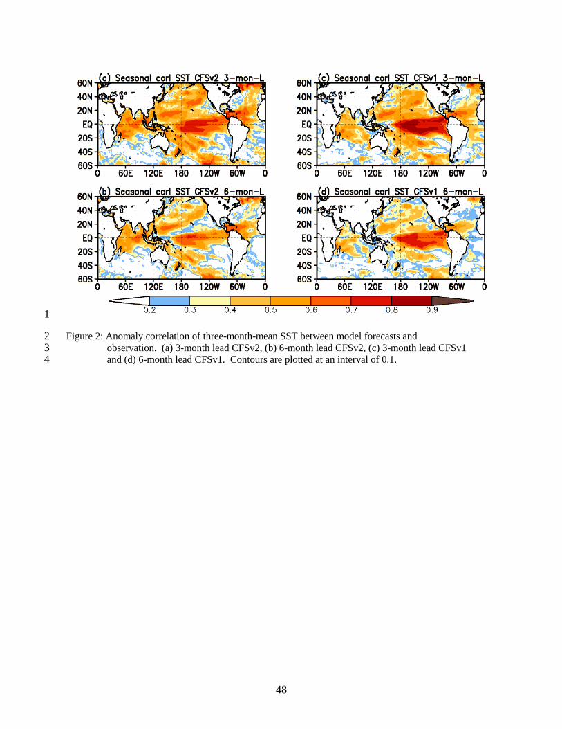
48

1

Figure 2: Anomaly correlation of three-month-mean SST between model forecasts and 2 observation. (a) 3-month lead CFSv2, (b) 6-month lead CFSv2, (c) 3-month lead CFSv1 3 and (d) 6-month lead CFSv1. Contours are plotted at an interval of 0.1. 4

49

1 Figure 3: Standard deviation of three-month-mean SST forecasts (K). (a) Observation (b) 3- 2 month lead CFSv2 minus observation, (c) 6-month lead CFSv2 minus observation, (d) 3- 3 month lead CFSv1 minus observation, and (e) 6-month lead CFSv1 minus observation 4

Contours are plotted at an interval of 0.2 from 0.2 to 1.6 in (a) and from -0.5 to 0.5 in (b), 5 (c), (d) and (e). 6

50

1 Figure 4: Evaluation of anomaly correlation as a function of target month (horizontal axis) and forecast 2

lead (vertical axis). On the left is CFSv1, on the right CFSv2. Top row shows monthly 2-meter 3 temperature over NH land, middle row shows monthly precipitation over NH land and the 4 bottom row shows the SST in the Nino3.4 area. The scale is the same for all 6 panels. Except 5 for the years added, the CFSv1 entries in this figure (left column) should correspond to the 6 figures in S06. 7

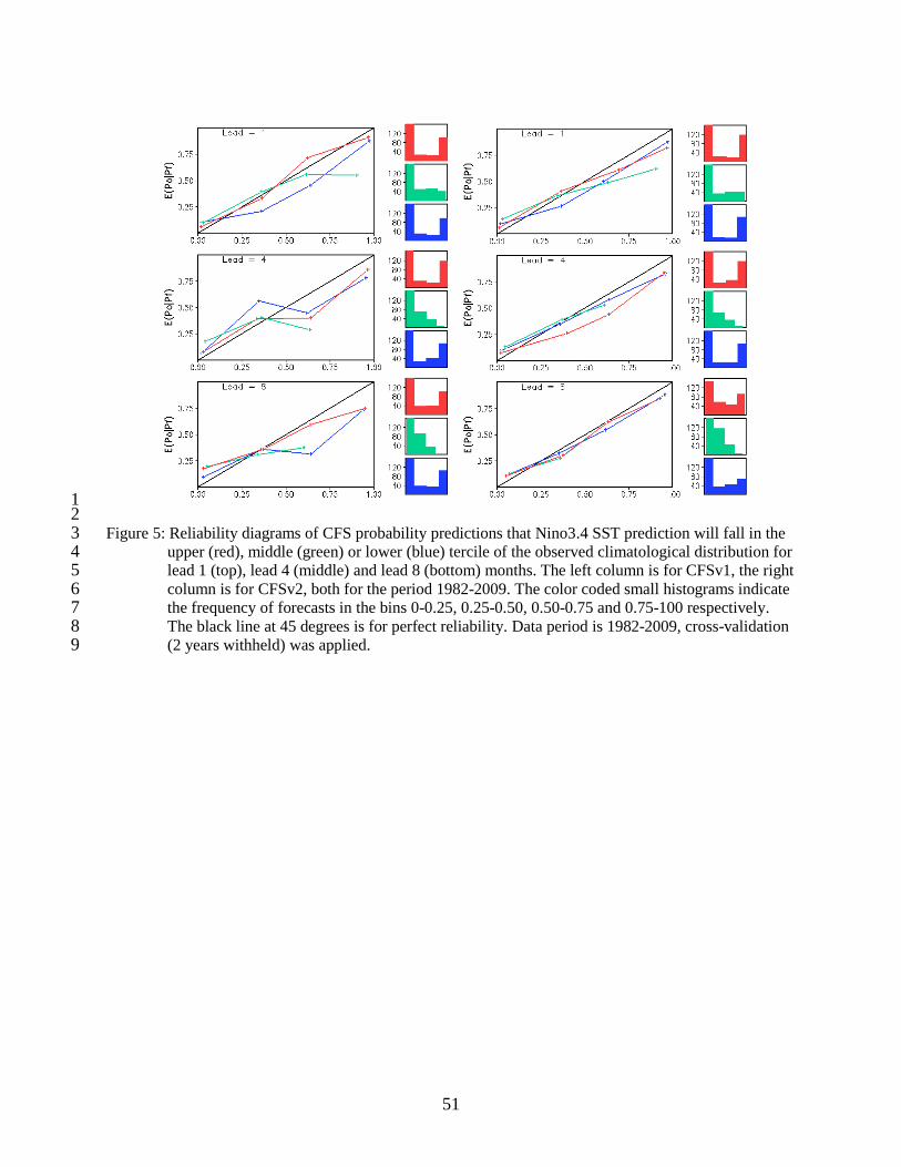
51

1 2

Figure 5: Reliability diagrams of CFS probability predictions that Nino3.4 SST prediction will fall in the 3 upper (red), middle (green) or lower (blue) tercile of the observed climatological distribution for 4 lead 1 (top), lead 4 (middle) and lead 8 (bottom) months. The left column is for CFSv1, the right 5 column is for CFSv2, both for the period 1982-2009. The color coded small histograms indicate 6 the frequency of forecasts in the bins 0-0.25, 0.25-0.50, 0.50-0.75 and 0.75-100 respectively. 7 The black line at 45 degrees is for perfect reliability. Data period is 1982-2009, cross-validation 8 (2 years withheld) was applied. 9

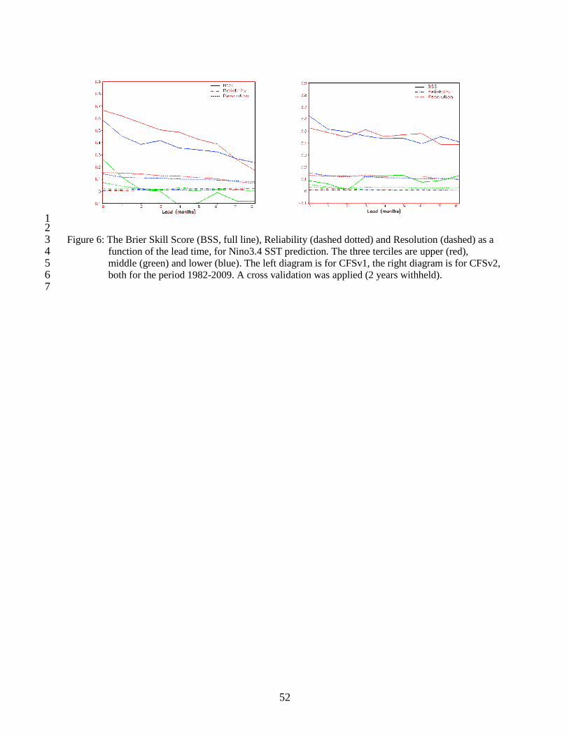
52

1 2 Figure 6: The Brier Skill Score (BSS, full line), Reliability (dashed dotted) and Resolution (dashed) as a 3

function of the lead time, for Nino3.4 SST prediction. The three terciles are upper (red), 4 middle (green) and lower (blue). The left diagram is for CFSv1, the right diagram is for CFSv2, 5 both for the period 1982-2009. A cross validation was applied (2 years withheld). 6

7

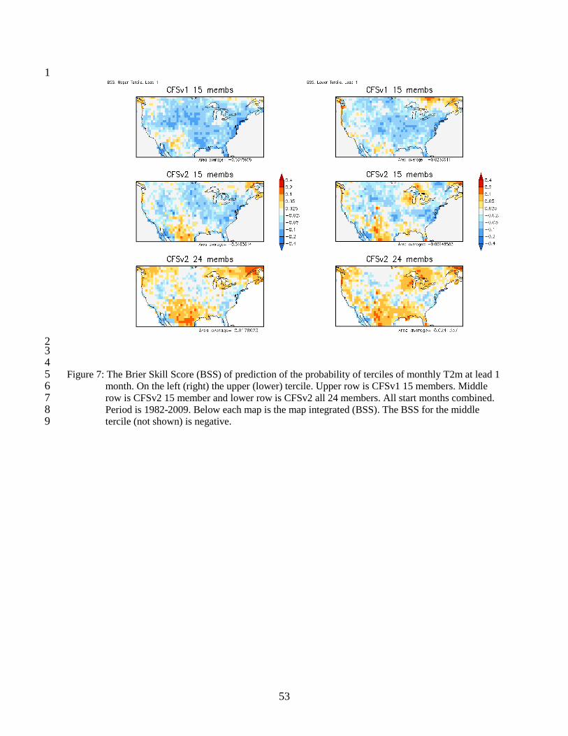
53

1

2 3 4

Figure 7: The Brier Skill Score (BSS) of prediction of the probability of terciles of monthly T2m at lead 1 5 month. On the left (right) the upper (lower) tercile. Upper row is CFSv1 15 members. Middle 6 row is CFSv2 15 member and lower row is CFSv2 all 24 members. All start months combined. 7 Period is 1982-2009. Below each map is the map integrated (BSS). The BSS for the middle 8 tercile (not shown) is negative. 9

54

1 2 Figure 8: The annual mean systematic error in three parameters (SST, T2m and Prate) at lead 3 evaluated 3

as the difference between the predicted and observed climatology for the full period 1982-2009. 4 Column on the left (right) is for CFSv1 (CFSv2). The header in each panel contains the root- 5 mean-square difference, as well as the spatial mean difference. Units are K for SST and T2m, 6 and mm/day for prate. Contours and colors as indicated by the bar underneath. 7

55

1

2 3 Figure 9: The annual mean systematic error in three parameters (SST, T2m and Prate) at lead 3 evaluated 4

as the difference between CFSv2‟s predicted and observed climatology. Column on the left 5 (right) is for 1982-1998 (1999-2009). The header in each panel contains the root-mean-square 6 difference, as well as the spatial mean difference. Units are K for SST and T2m, and mm/day 7 for prate. Contours and colors as indicated by the bar underneath. 8

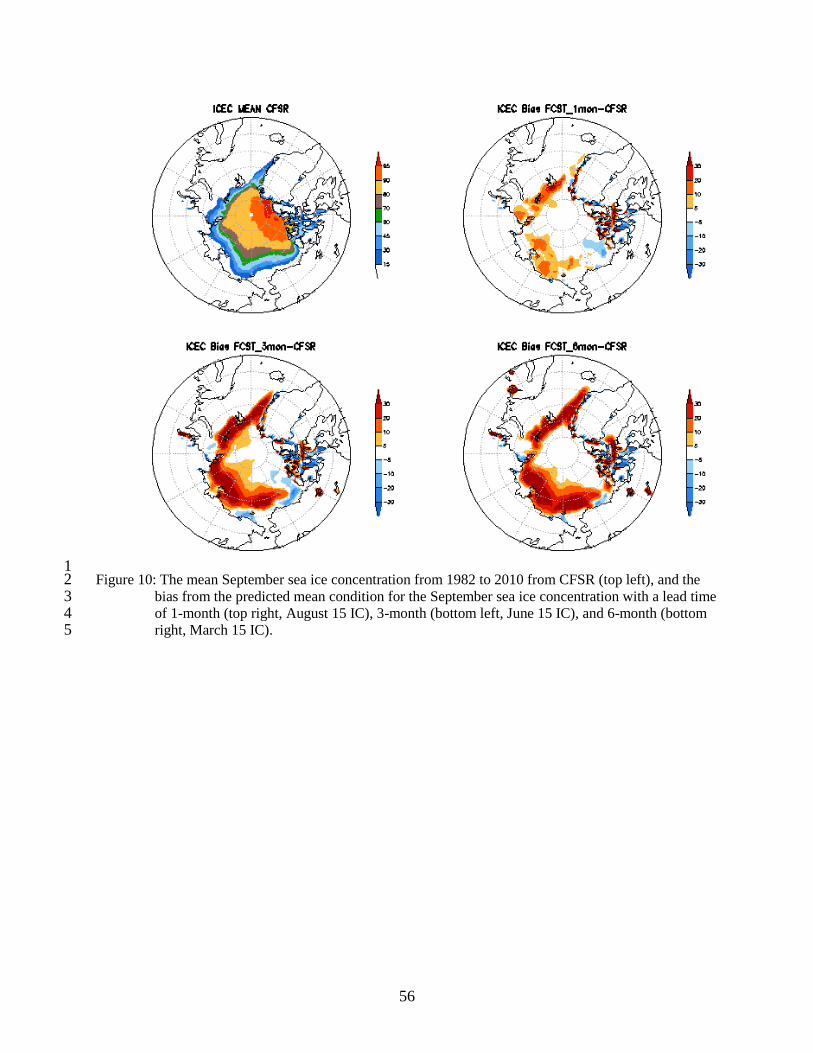
56

1 Figure 10: The mean September sea ice concentration from 1982 to 2010 from CFSR (top left), and the 2

bias from the predicted mean condition for the September sea ice concentration with a lead time 3 of 1-month (top right, August 15 IC), 3-month (bottom left, June 15 IC), and 6-month (bottom 4 right, March 15 IC). 5

57

1 Figure 11: The standard deviation of the September sea ice concentration from 1982 to 2010 from CFSR 2 (top left), and the difference of the standard deviation between the model prediction and that 3 from the CFSR for the September sea ice concentration with a lead time of 1-month (top right, 4 August 15 IC), 3-month (bottom left, June 15 IC), and 6-month (bottom right, March 15 IC). 5

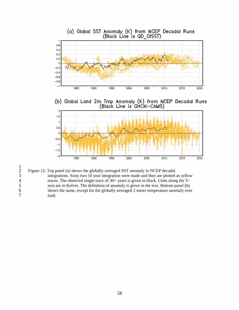
58

1 Figure 12: Top panel (a) shows the globally averaged SST anomaly in NCEP decadal 2

integrations. Sixty two 10 year integration were made and they are plotted as yellow 3 traces. The observed single trace of 30+ years is given in black. Units along the Y- 4 axis are in Kelvin. The definition of anomaly is given in the text. Bottom panel (b) 5 shows the same, except for the globally averaged 2 meter temperature anomaly over 6 land. 7

59

1

2 3 Figure 13: Power spectra of time series of monthly anomalies of the Nino34 index (average SST from 4

170W to 120W, and 5S to 5N). Upper left is for the observation while the other three 5 panels are for CMIP runs of 43, 52 and 100 years respectively. 6

60

1

2

3

4

5

6

7

8

9

10 Figure A1: Reforecast Configuration of the CFSv2 11

12

45 day run 1 season run

Jan 1

UTC

Jan 2 Jan 3

9 month run

Jan 5 Jan 4 Jan 6

61

1

2

3

4

5

6

7

8 Figure A2: Operational Configuration of the CFSv2 9

1 season run (3)

18 UTC 0 UTC 6 UTC 12 UTC

9 month run (4) 45 day run (9)