The new ECMWF Variable Resolution Ensemble Prediction ... · 499 The new ECMWF Variable Resolution Ensemble Prediction System (VAREPS): methodology and validation Roberto Buizza,

499

The new ECMWF Variable Resolution Ensemble Prediction

System (VAREPS): methodology and validation

Roberto Buizza, Jean-Raymond Bidlot, Nils Wedi, Manuel Fuentes, Mats Hamrud, Graham Holt,

Tim Palmer and Frederic Vitart

Research Department

July 2006

Series: ECMWF Technical Memoranda A full list of ECMWF Publications can be found on our web site under: http://www.ecmwf.int/publications.html [email protected] © Copyright 2006 European Centre for Medium Range Weather Forecasts Shinfield Park, Reading, Berkshire RG2 9AX, England Literary and scientific copyrights belong to ECMWF and are reserved in all countries. This publication is not to be reprinted or translated in whole or in part without the written permission of the Director. Appropriate non-commercial use will normally be granted under the condition that reference is made to ECMWF. The information within this publication is given in good faith and considered to be true, but ECMWF accepts no liability for error, omission and for loss or damage arising from its use.

http://www.ecmwf.int/publications.html

The new ECMWF VAREPS: methodology and validation

Technical Memorandum No.499 1

Abstract On the 1st of February 2006, the resolution of the European Centre for Medium-Range Weather Forecasts (ECMWF) Ensemble Prediction System (EPS) was increased from TL255L40 to TL399L62. This change was the first of a three-phase upgrading process that will lead to the implementation of the ECMWF Variable Resolution Ensemble Prediction System (VAREPS), a system designed to provide skilful predictions of small-scale, severe-weather events in the early forecast range, and accurate forecast large-scale guidance in the medium forecast range.

In this work, first the rationale behind VAREPS is presented, and then average results based on a VAREPS with a truncation at forecast day 7 and 40 vertical levels [i.e. TL399L40(d0-7) and TL255L40(d7-15)] are discussed, and compared to the performance of two constant resolution systems, a TL255L40 and a TL319L40 (this latter one requires similar computing resources to VAREPS).

Average results based on 111 cases indicate that VAREPS is more skilful than a TL255L40 EPS, and that VAREPS should be preferred to the constant-resolution TL319L40 EPS, since it provides significantly better forecasts in the early forecast range without loosing accuracy in the long forecast range. The differences between VAREPS and the other two systems are, on average, small, but statistically significant in the early forecast range. The discussion of some specific events indicate that that these differences can be very large, and can lead to substantial improvements in the prediction of severe weather events, such as the ones linked with hurricanes, or intense precipitation. Results have also shown that VAREPS will be able to provide some skilful forecasts beyond forecast day 10.

VAREPS will further increase the value of the ECMWF probabilistic forecasting system, and deliver more accurate predictions of small-scale, severe weather events in the early forecast range and skilful probabilistic predictions of larger scale features in the medium forecast range.

1. The ECMWF approach to ensemble prediction The Ensemble Prediction System (EPS) has been part of the ECMWF operational suite since December 1992. At that time, the EPS was based on 33 forecasts produced with a T63L19 (spectral triangular truncation T63 with 19 vertical levels) resolution version of the ECMWF model (Molteni et al., 1996). The initial uncertainties were simulated by starting 32 members from perturbed initial conditions defined by T21L31 perturbations which are rapidly-growing during the first 36 hours of the forecast range (the singular vectors, see Buizza & Palmer, 1995).

Since December 1992, the EPS has been upgraded several times. During these years, the EPS has used the same model version as the data assimilation and forecast system, benefiting from all the changes made. Some of these changes included substantial modifications of the EPS configuration, designed to improve both the simulation of initial and model uncertainties. It is worth identifying a few of them:

• In 1994 the optimisation time interval of the singular vectors was extended to 48 hours.

• In 1995 the singular vectors’ resolution was increased to T42L31.

• In 1996 the system was upgraded to a 51-member TL159L31 system (spectral triangular truncation T159 with linear grid; Buizza et al., 1998), with T42L31 singular vectors.

• In 1998, initial uncertainties due to perturbations that had grown during the 48 hours previous to the starting time (evolved singular vectors, Barkmeijer et al., 1999) were included, and a scheme to simulate model uncertainties due to random model error in the parameterized physical processes was


2 Technical memorandum No.499

introduced (Buizza et al., 1999). EPS wave forecasts became available following the introduction of the coupled atmosphere-wave model in the forecast model (Saetra & Bidlot, 2004, Janssen et al., 2005).

• In 2000, following the resolution increase of the ECMWF data-assimilation and high-resolution systems from TL319L31 to TL511L60, the EPS resolution was upgraded to TL255L40 (Buizza et al., 2003), with T42L40 singular vectors. The wave model resolution was increased to a grid spacing of the order of 110 km.

• In 2002, tropical perturbations were added to the system (Barkmeijer et al., 2001).

• In 2004, the Gaussian sampling method for generating the EPS initial perturbations using singular vectors was implemented (Ehrendorfer & Beck, 2003).

• On 1 February 2006, following another resolution increase of the ECMWF data-assimilation and high-resolution systems to TL799L90, the EPS resolution was further increased to TL399L62, with T42L62 singular vectors. The wave model spectral resolution was increased to 30 frequencies and 24 directions respectively without any change to its horizontal resolution.

The most recent change is the first of a three-phase upgrading process that will lead to the implementation of the ECMWF Variable Resolution Ensemble Prediction System (VAREPS). VAREPS has been designed to benefit from an increased resolution in the early forecast range and from an extension of the forecast range initially to 15 days and eventually to one month with the merger of the medium-range ensemble and the monthly operational system:

• Phase 1 (February 2006): resolution increase of the 10-day EPS from TL255L40 to TL399L62.

• Phase 2 (planned for the second half of 2006): extension of the forecast range to 15 days using the VAREPS system, with TL399L62(d0-10) and TL255L62(d10-15).

• Phase 3 (planned for 2007): weekly extension of VAREPS to one month, with a TL255L62 atmospheric resolution and ocean coupling introduced at day 10 (the precise configuration of this final stage of VAREPS is still to be finalized).

In this article, the performance of VAREPS is compared to the performance of two constant-resolution ensemble systems, one with the resolution used in the operational EPS before 1 February 2006 (i.e. TL255L40) and one with a TL319L40 resolution. The comparison between this latter system and VAREPS is particularly interesting, because the two systems require a similar amount of computing resources but they are fundamentally different in the design, and will highlight the advantages of a variable resolution approach to ensemble prediction. After this introduction, section 2 will present the rationale behind VAREPS, section 3 will discuss some average results and section 4 will compare the performance of different ensemble systems for some cases of extreme weather. Finally, section 5 will summarize the key results of this work.



2. The rationale behind a variable resolution approach Given a certain amount of computer resources, VAREPS has been designed (a) to resolve the smallest possible scales up to the forecast time when their inclusion has a positive impact on the prediction of both the small and the synoptic scales, and (b) not to resolve them later in the forecast range when including them has a smaller, less detectable impact on the synoptic scales. This approach leads to a more cost-efficient use of the computer resources, with most of them used in the early forecast range to resolve the small but still predicable scales. It is worth noting that a similar approach to ensemble prediction is not new, since it has been used at the National Centers for Environmental Prediction (NCEP, Washington) since inception of their ensemble prediction system (Toth & Kalnay 1997).

2.1 VAREPS technical configuration The VAREPS system used in the experimentation discussed in this work used 40 vertical levels and a truncation from high- to low-resolution at forecast day 7, i.e. the two legs of each forecast had the following characteristics:

• leg-1: TL399L40, from day 0 to day 7.

• leg-2: TL255L40, from day 6 to day 15.

The horizontal resolution of the wave model remains unchanged (~110 km) in the two legs; however leg-1 is now run with the same spectral resolution as the deterministic forecast (30 frequencies and 24 directions). The second leg reverts to 25 frequencies and 12 directions.

It should be noted that of the 111 cases, 49 cases have been run for with a forecast length of 15 days, 40 with a forecast length of 14 days and 22 with a forecast length of 13 days: thus, when 111-case averages are shown they will be limited to a 13-day forecast length, so that all cases can be included.

2.2 Key VAREPS technical characteristics It is worth highlighting three key technical characteristics of VAREPS:

• Leg-2 initial conditions – Each leg-2 forecast starts from a leg-1 day-6 forecast (Fig. 1), interpolated at the TL255L62 resolution. The 24-hour overlap period has been introduced to reduce the impact on the fields that are more sensitive to the truncation from the high to the low resolution (e.g. convective and large scale precipitation). High resolution wave spectra are smoothed out to the lower spectral resolution of the second leg.



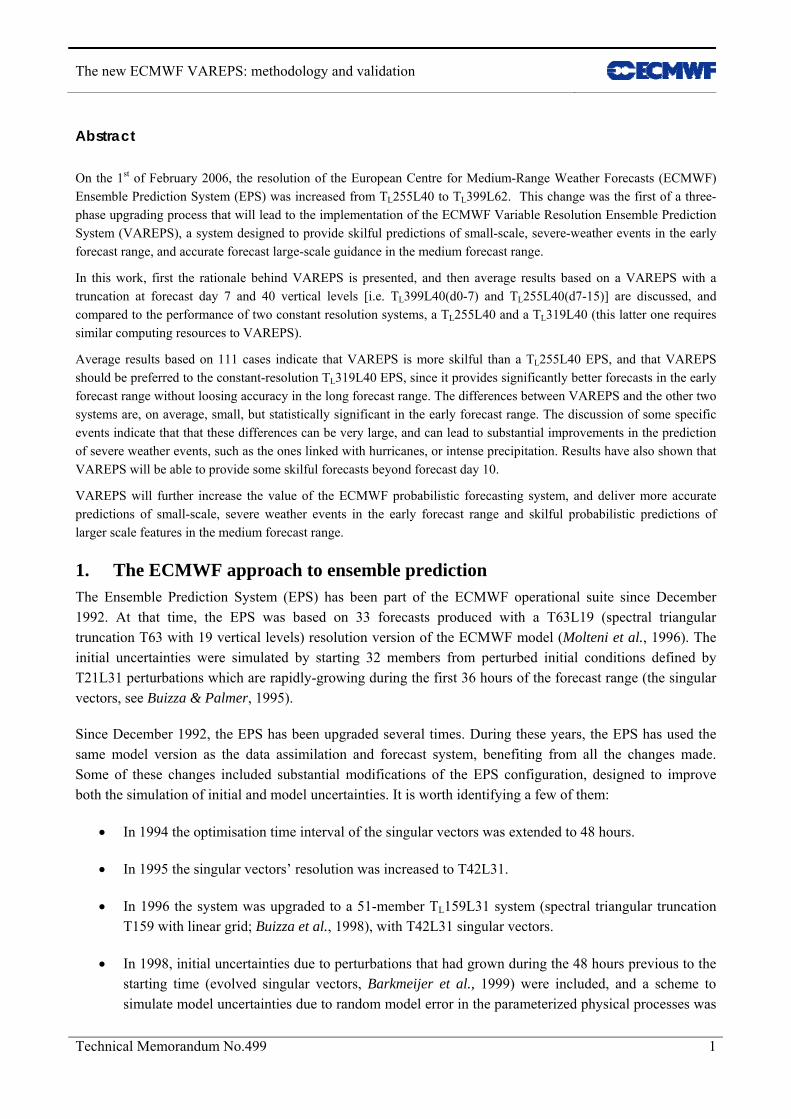
Figure 1 Schematic of the 2-leg VAREPS used in this experimentation, with MARS data streams ENFO and EFOV.

• Accumulated fields – Accumulated fields are accumulated from the start of the leg-1 forecast. To accumulate from the start of leg-1 throughout the forecast of all legs, once each leg-2 forecast reaches the end of the overlap period (24-hour, i.e. day-7 if counted from the beginning of the leg-1 forecast), the accumulated fields are re-set to be equal to the leg-1 day-7 forecast fields interpolated on the TL255 reduced Gaussian grid.

• Archived fields – To avoid that forecasts generated by leg-2 overwrite fields generated by leg-1, leg-1 forecasts from day 0 to the truncation forecast time (i.e. day 7), and leg-2 forecasts from the truncation forecast time to the end of the forecast period (i.e. from day 7 to day 15) are written in the ECMWF Meteorological Archival and Retrieval System (MARS) in stream ENFO (Ensemble Forecast stream), while leg-2 forecasts from the beginning of leg-2 to the truncation forecast time (i.e. from forecast day 6 to 7) are written in the new MARS stream EFOV (Ensemble Forecast OVeralp stream). Similarly, ensemble wave fields are written in, respectively, streams WAEF and WEOV.

This set-up ensures that only users interested in using VAREPS forecast for accumulated fields after the truncation forecast time need to take care when constructing fields accumulated between two forecast steps that include the truncation step (see Appendix A for more details).

3. Expected average impact of the introduction of VAREPS The performance of VAREPS has been compared with the performance of two contant resolution ensemble systems, one with the same characteristics as the EPS operational up to the 1st of February 2006 but extended to forecast day 15, and one with a TL319L40 resolution:

• T255: TL255L40(day 0–13), with a 2700 second time step (this was the EPS configuration operational before 1 February 2006).

• VAREPS: TL399L40(day 0–7) with a 1800 second time step and TL255L40(day 6–13) with a 2700 second time step.

• T319: TL319L40(day 0–13) with a 1800 second time step.

STEP=0 144 168 360

T399

T255

LEG 1: LEG 2: MARS stream=ENFO: MARS stream=EFOV:

T399 T255



The second and the third configurations require ~3.5 times the computing requirements of the first configuration. Apart from the resolution, these ensembles used the same model cycle, started from the same analysis, had the same set of initial perturbations and were based on 50 perturbed plus 1 unperturbed forecast. 51-member ensemble forecasts from the first two configurations have been generated for 111 cases, spanning different years and different seasons, and including an un-biased set of atmospheric situations. Due to limited computing resources, ensembles in configuration T319 have been run only for 89 of the 111 cases only (unfortunately, it has not been possible to extend these data set; it is worth quoting that these experiments used the equivalent of the computer resources required to run a 10-day TL511L60 forecast for 10 years!).

Verification has been focused mainly on three forecast fields: the 500 hPa geopotential height (Z500), the 850 hPa temperature (T850), and 12-hour accumulated total precipitation (TP12), defined on a 2.5 degree regular latitude/longitude grid; mean sea level pressure (MSLP) and significant-wave-height (SWH) have also been considered for some specific case studies. For all but total precipitation, the ECMWF operational analysis has been used as verification; for total precipitation, 0-to-12 and 12-to-24-hour forecasts from the ECMWF operational, high-resolution forecast has been used as an approximated verification field.

Single and probabilistic forecasts have been assessed using a range of accuracy measures, including the ranked probability skill score (RPSS, Wilks 1995), computed with respect to climatology, the Brier skill score (BSS, Brier 1950) and the area under the relative operating characteristic curve (ROCA) computed in terms of the standard normal deviates (Swets 1982, Wilson 2000). Statistical significance has been assessed considering the non-parametric rank-sum Mann-Whitney-Wilcoxon test (Wilks 1995). Given the distributions of forecast scores for two ensemble prediction systems EPS1 and EPS2, the rank-sum test measures the probability that the distributions of scores of EPS1 and EPS2 come from the same overall population: for example, a rank-sum values of 20% indicate that there is a 20% chance that the distributions of the two scores coincide (see Append B for more details on how the test value has been computed).

3.1 Comparison of T255 EPS and VAREPS Figure 2 shows the 111-case average RPSS and the area under the relative operating characteristic curve for the probabilistic prediction of total precipitation for the T255 and the VAREPS systems, and the corresponding value of the rank-sum test. Figure 2 shows that VAREPS has higher average scores than T255 up to forecast day 7, with rank-sum test values below 20% up to forecast day 6, while differences beyond forecast day 6 becomes smaller, with the rank-rum test reaching values above 20%.



RPSS - TP12 NH (111 cases)

0.0

0.1

0.2

0.3

0.4

0.5

0 1 2 3 4 5 6 7 8 9 10 11 12 13Forecast day

0

10

20

30

40

50

T255VAREPSRMW

ROCAZ - PR(TP12>5mm) NH (111 cases)

0.70

0.75

0.80

0.85

0.90

0.95

1.00

0 1 2 3 4 5 6 7 8 9 10 11 12 13Forecast day

0

10

20

30

40

50

60

'T255VAREPSRMW

ROCAZ - PR(TP12>10mm) NH (111 cases)

0.70

0.75

0.80

0.85

0.90

0.95

1.00

0 1 2 3 4 5 6 7 8 9 10 11 12 13Forecast day

0

10

20

30

40

50

60

T255VAREPSRMW

Figure 2 Top panel:average (111-cases) ranked probability skill score over Northern Hemisphere for EPS (solid greyline, left axis) and VAREPS (solid black line, left axis), and rank-sum Mann-Whitney-Wilcoxon significance test (dotted line, right axis). Middle: as top panel but for the area under the relative operating characteristic curve for the probabilistic prediction of total precipitation in excess of 5 mm/12h. Bottom panel: as middle panel but for the probabilistic prediction of total precipitation in excess of 10 mm/12h.

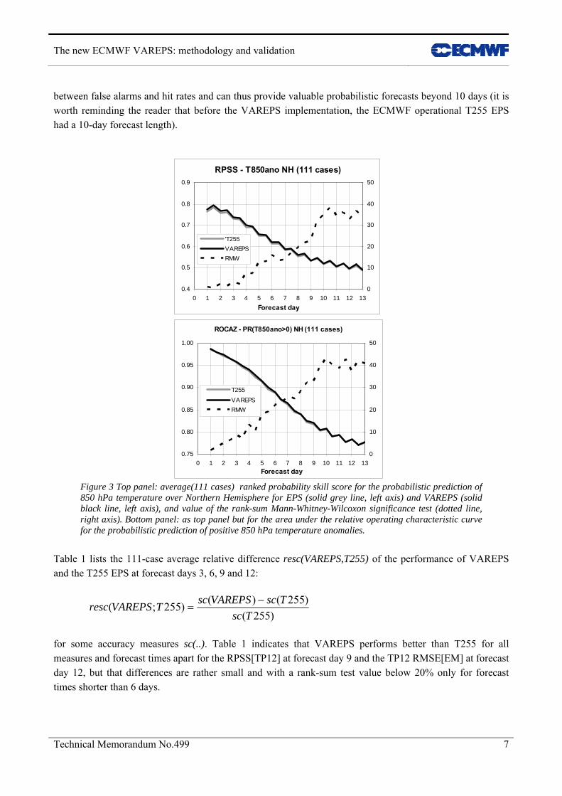
Figure 3 shows the corresponding 111-case average results for T850 (RPSS, and ROCA for the probabilistic prediction of positive anomalies). Results indicate that the difference between these two systems in terms of the prediction of T850 are smaller but still with a rank-rum test with values below 20% up to forecast day 7.5 if one considers the RPSS, and day 5.5 if one considers ROCA. It is worth pointing out that for VAREPS ROCA stays above 0.75 for the whole forecast range, indicating that the system is capable to discriminate



between false alarms and hit rates and can thus provide valuable probabilistic forecasts beyond 10 days (it is worth reminding the reader that before the VAREPS implementation, the ECMWF operational T255 EPS had a 10-day forecast length).

RPSS - T850ano NH (111 cases)

0.4

0.5

0.6

0.7

0.8

0.9

0 1 2 3 4 5 6 7 8 9 10 11 12 13Forecast day

0

10

20

30

40

50

'T255VAREPSRMW

ROCAZ - PR(T850ano>0) NH (111 cases)

0.75

0.80

0.85

0.90

0.95

1.00

0 1 2 3 4 5 6 7 8 9 10 11 12 13Forecast day

0

10

20

30

40

50

T255VAREPSRMW

Figure 3 Top panel: average(111 cases) ranked probability skill score for the probabilistic prediction of 850 hPa temperature over Northern Hemisphere for EPS (solid grey line, left axis) and VAREPS (solid black line, left axis), and value of the rank-sum Mann-Whitney-Wilcoxon significance test (dotted line, right axis). Bottom panel: as top panel but for the area under the relative operating characteristic curve for the probabilistic prediction of positive 850 hPa temperature anomalies.

Table 1 lists the 111-case average relative difference resc(VAREPS,T255) of the performance of VAREPS and the T255 EPS at forecast days 3, 6, 9 and 12:

)255(

)255()()255;(Tsc

TscVAREPSscTVAREPSresc −=

for some accuracy measures sc(..). Table 1 indicates that VAREPS performs better than T255 for all measures and forecast times apart for the RPSS[TP12] at forecast day 9 and the TP12 RMSE[EM] at forecast day 12, but that differences are rather small and with a rank-sum test value below 20% only for forecast times shorter than 6 days.



Variable Measure Day 3 Day 6 Day 9 Day 12 RMSE(EM) 0.43 ( 2.6) 0.62 (17.0) 0.45 (28.6) 0.35 (39.1) RPSS[T850ano] 1.10 ( 3.34) 1.14 (16.2) 0.75 (22.9) 0.61 (32.9) T850 ROCA[T850ano>0] 0.20 ( 8.60) 0.33 (18.2) 0.24 (32.8) 0.26 (37.5) RMSE(EM) 0.10 (22.6) 0.63 (28.7) 1.0 (34.3) 0.47 (42.3) RPSS[Z500ano] 0.38 (20.0) 0.61 (37.2) 0.90 (32.2) 0.39 (37.6) Z500 ROCA[Z500ano>0] 0.10 (14.2) 0.22 (29.4) 0.25 (24.9) 0.27 (37.2) RMSE(EM) 1.72 (31.2) 0.53 (40.0) 0.00 (47.5) -0.26 (48.8) RPSS[TP12] 6.51 ( 3.1) 4.05 (12.5) -0.74 (42.8) 0.00 (48.6) TP12 ROCA[TP12>5mm] 0.55 ( 4.8) 1.10 ( 9.7) 0.00 (47.0) 0.13 (27.0)

Table 1 Summary of the average (111 cases) relative difference (sc[VAREPS]-sc[EPS])/sc[EPS] over the Northern Hemisphere (NH) of VAREPS and EPS at forecast days 3, 6, 9 and 12, for 850 hPa temperature (T850), 500 hPa geopotential height (Z500) and 12h accumulated total precipitation (TP). Relative differences and rank-sum Mann-Withney-Wilcoxon values (RMW, in brackets) are expressed in percentages. Positive values indicate that VAREPS outperforms EPS; bold identifies values with RMW<20%.

Thus, results based on 111 cases indicate that the impact of increasing the forecast resolution in the first 7-days in VAREPS is on average positive and statistically significant (in the sense that the rank-sum test has values below 20%) in the earlier forecast range, with differences more evident for forecast variables close to the surface, such as total precipitation and T850.

3.2 Comparison of T319 EPS and VAREPS It is interesting to compare the relative improvement (with respect to the T255 EPS) of the two ensemble configurations that require the same amount of computing resources to be completed: VAREPS and the constant resolution T319 ensemble system. Figure 4 shows the relative differences between average RPSSs (computed for 89 of the 111 cases shown in Figures 2 and 3) for TP12, and the corresponding rank-sum test values.

Diff RPSS (Tx-T255) - TP12 NH (89 cases)

-4.0%

-2.0%

0.0%

2.0%

4.0%

6.0%

8.0%

0 1 2 3 4 5 6 7 8 9 10 11 12 13

Forecast day

(T319-T255)/T255

(VAREPS-T255)/T255

Diff RPSS (Tx-T255) - TP12 NH (89 cases)

05

101520253035404550

0 1 2 3 4 5 6 7 8 9 10 11 12 13Forecast day

RMW(T255,T319)

RMW(T255,VAREPS)

Figure 4 Left panel: relative differences,[RPSS(Tx)-RPSS(T255)]/RPSS(T255), between the average (89 cases) ranked probability skill score for the probabilistic prediction of total precipitation over Northern Hemisphere of VAREPS and T255 (black line) and (T319-T255) (grey line). Right panel: as left panel but for the rank-sum Mann-Whitney-Wilcoxon statistical test (RMW).



On average, results indicate that while the relative difference is positive for VAREPS almost for all forecast steps, it becomes negative for T319 after forecast day 4. Considering the rank-sum test, it is worth pointing out that while the test has values below 20% for VAREPS versus T255 up to forecast day 5.5, it is almost always above 20% for T319 versus T255: this indicates that the differences between the distributions of RPSSs of T319 and T255 are not statistically significant.

Similar conclusions can be drawn by comparing the relative differences between average RPSSs for T850 and the corresponding rank-sum test values (Fig. 5). Figure 5 confirms that the differences between VAREPS and T255 are larger and more statistically significant than the differences between T319 and T255.

Tables 2 and 3 list, for the accuracy measures sc(..) reported in Table 1, the 89-case average relative difference resc(xx,T255) of the performance of VAREPS and the T255 EPS, and the T319 and the T255 EPS, at forecast days 3, 6, 9 and 12. These tables confirm the main conclusion that was drawn from Figures 4 and 5: VAREPS performs, on average, better than the T319 EPS, especially in the early forecast range and for variable close to the surface.

Variable Measure Day 3 Day 6 Day 9 Day 12 RMSE(EM) 0.32 ( 7.7) 0.62 (21.5) 0.44 (28.9) 0.17 (45.8) RPSS[T850ano] 0.95 (10.0) 0.97 (24.3) 0.75 (33.3) 0.40 (40.3) T850 ROCA[T850ano>0] 0.21 (12.1) 0.22 (23.4) 0.12 (33.8) 0.13 (40.0) RMSE(EM) 0.10 (22.6) 0.63 (28.7) 1.0 (34.3) 0.47 (42.3) RPSS[Z500ano] 0.37 (26.2) 0.77 (38.0) 0.72 (38.0) 0.19 (41.8) Z500 ROCA[Z500ano>0] 0.10 (19.3) 0.22 (30.4) 0.25 (29.2) 0.27 (40.2) RMSE(EM) 1.42 (37.0) 0.79 (43.3) 0.00 (49.1) 0.00 (47.4) RPSS[TP12] 5.98 ( 6.7) 4.57 (13.4) 0.00 (47.0) 0.00 (45.2) TP12 ROCA[TP12>5mm] 0.55 ( 9.9) 1.10 (16.5) -0.39 (49.0) 0.54 (24.1)

Table 2. Summary of the average (89 cases) relative difference (sc[VAREPS]-sc[EPS])/sc[EPS] over the Northern Hemisphere (NH) of VAREPS and EPS at forecast days 3, 6, 9 and 12, for 850 hPa temperature (T850), 500 hPa geopotential height (Z500) and 12h accumulated total precipitation (TP). Relative differences and rank-sum Mann-Withney-Wilcoxon values (RMW, in brackets) are expressed in percentages. Positive values indicate that VAREPS outperforms T319; bold identifies values with RMW<20%.

Variable Measure Day 3 Day 6 Day 9 Day 12 RMSE(EM) 0.21 (14.1) 0.25 (40.4) 0.15 (36.3) 0.17 (41.4) RPSS[T850ano] 0.68 (16.8) 0.49 (40.0) 0.19 (47.3) 0.40 (44.4) T850 ROCA[T850ano>0] 0.21 ( 9.8) 0.11 (31.7) -0.12 (44.7) -0.13 (44.7) RMSE(EM) 0.00 (44.1) 0.13 (44.6) -0.34 (47.3) -1.17 (45.1) RPSS[Z500ano] 0.12 (46.7) 0.15 (47.6) -0.18 (45.6) -0.58 (38.9) Z500 ROCA[Z500ano>0] 0.00 (34.3) 0.00 (46.7) -0.25 (42.3) -0.14 (42.1) RMSE(EM) 0.28 (49.4) -0.26 (49.0) 0.25 (45.0) 0.51 (40.5) RPSS[TP12] 0.98 (42.9) -0.57 (42.4) -2.21 (19.9) -3.20 (23.4) TP12 ROCA[TP12>5mm] 0.44 (21.6) 0.37 (33.3) -0.51 (40.3) 0.27 (40.5)

Table 3. Summary of the average (89 cases) relative difference (sc[T319]-sc[EPS])/sc[EPS] over the Northern Hemisphere (NH) of VAREPS and EPS at forecast days 3, 6, 9 and 12, for 850 hPa temperature (T850), 500 hPa geopotential height (Z500) and 12h accumulated total precipitation (TP). Relative differences and rank-sum Mann-Withney-Wilcoxon values (RMW, in brackets) are expressed in percentages. Positive values indicate that VAREPS outperforms T319; bold identifies values with RMW<20%.



Diff RPSS (Tx-T255) - T850 NH (89 cases)

-0.2%

0.0%

0.2%

0.4%

0.6%

0.8%

1.0%

1.2%

0 1 2 3 4 5 6 7 8 9 10 11 12 13

Forecast day

(T319-T255)/T255

(VAREPS-T255)/T255

Diff RPSS (Tx-T255) - T850 NH (89 cases)

05

101520253035404550

0 1 2 3 4 5 6 7 8 9 10 11 12 13

Forecast day

RMW(T255,T319)

RMW(T255,VAREPS)

Figure 5 Left panel: relative differences,[RPSS(Tx)-RPSS(T255)]/RPSS(T255), between the average (89 cases) ranked probability skill score for the probabilistic prediction of 850 hPa temperature anomalies over Northern Hemisphere of VAREPS and T255 (black line) and (T319-T255) (grey line). Right panel: as left panel but for the rank-sum Mann-Whitney-Wilcoxon statistical test (RMW).

4. Impact of increased resolution in the short-range for selected cases The average results discussed in section 3 have indicated that the differences between VAREPS and the T255 EPS (which was the operational system operational until the 31st of January 2006) are very small but with a rank-sum test value below 20% up to forecast day 6, especially for variables close to the surface. Results have also indicated that VAREPS is to be preferred to a constant resolution, equal cost TL319 ensemble.

In this section, first the value of the VAREPS increased resolution in the early forecast range is investigated in three cases of severe weather, and then the value of VAREPS forecast range extension to 15 days is investigated in two summer case.

4.1 Hurricane Katrina (29 August 2005): mean-sea-level-pressure and significant wave height prediction

The first case is very recent: hurricane Katrina, one of the strongest storms of the last 100 years. Katrina started to develop as a tropical depression on 23 August south-east of the Bahamas, reached category 5 on 28 August and category 4 when it landed on the 29th. At landfall, close to New Orleans, sustained winds of more than 220 km/h were detected.

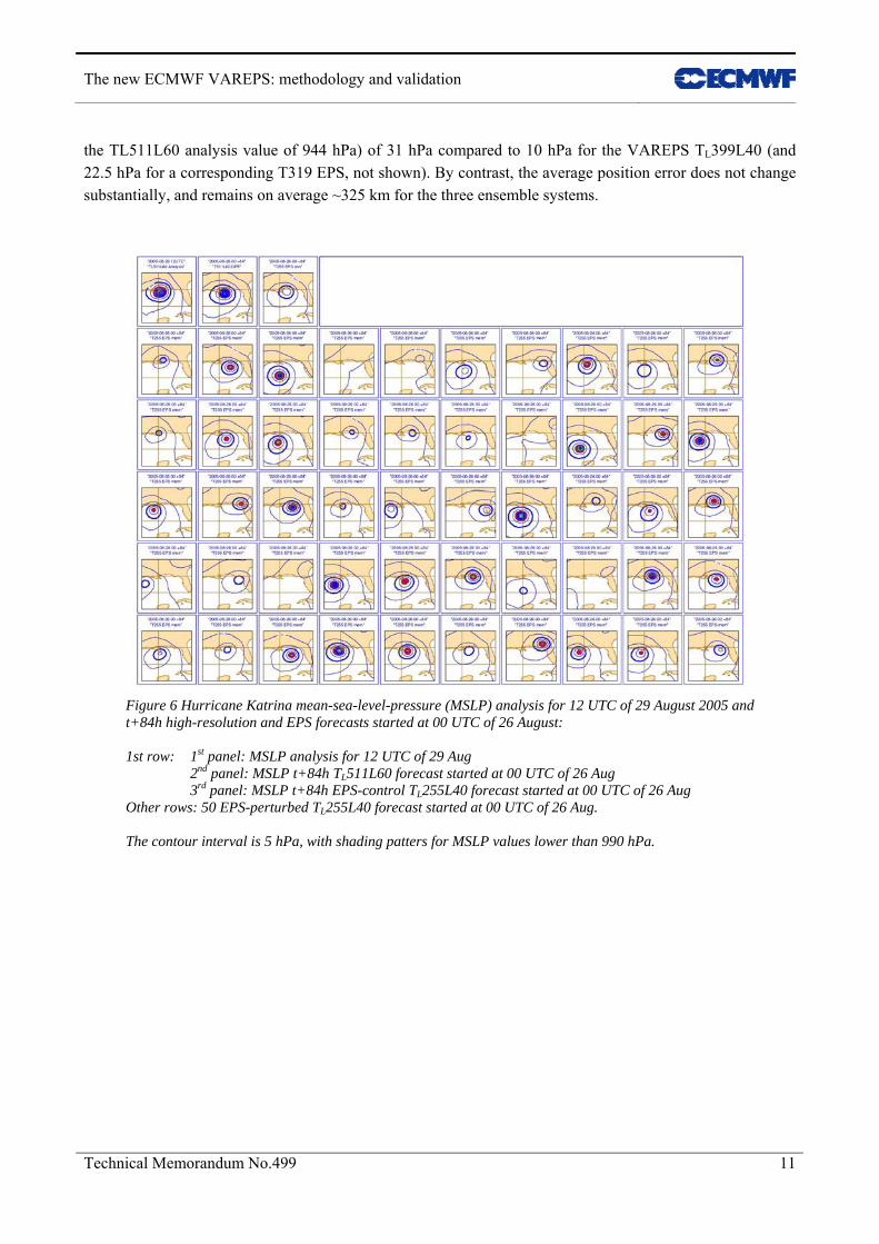
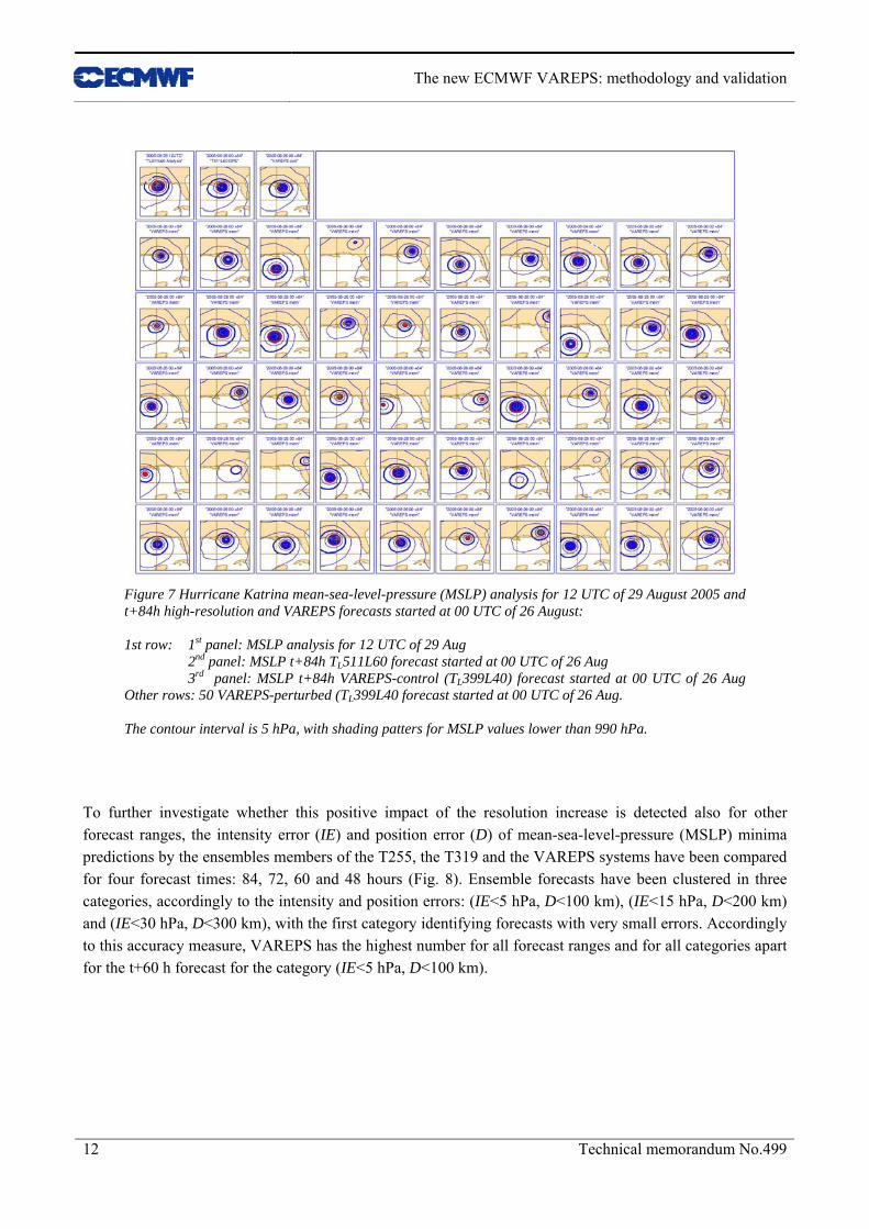
Figure 6 shows the mean-sea-level-pressure (MSLP) t+84h forecasts from the T255 EPS started at 00 UTC of the 26th of August, and valid for 12 UTC of the 29th of August, the time of Katrina’s landfall close to New Orleans. The first three top panels of Figure 6 show the ECMWF operational analysis, and the operational TL511L60 and the TL255L40 EPS-control forecasts, while the other 50 panels show the EPS perturbed forecasts. Figure 6 shows that few EPS members correctly predict the position of the hurricane, but that in general these forecasts were producing a system that was too weak. Figure 7 shows the corresponding VAREPS TL399L40 forecasts, with many more members predicting an intense system. A closer comparison of the corresponding members confirm that the VAREPS TL399L40 predicted cyclones were deeper than the corresponding T255 EPS predicted ones, with an average MSLP intensity error (computed with respect to



the TL511L60 analysis value of 944 hPa) of 31 hPa compared to 10 hPa for the VAREPS TL399L40 (and 22.5 hPa for a corresponding T319 EPS, not shown). By contrast, the average position error does not change substantially, and remains on average ~325 km for the three ensemble systems.

Figure 6 Hurricane Katrina mean-sea-level-pressure (MSLP) analysis for 12 UTC of 29 August 2005 and t+84h high-resolution and EPS forecasts started at 00 UTC of 26 August: 1st row: 1st panel: MSLP analysis for 12 UTC of 29 Aug 2nd panel: MSLP t+84h TL511L60 forecast started at 00 UTC of 26 Aug 3rd panel: MSLP t+84h EPS-control TL255L40 forecast started at 00 UTC of 26 Aug Other rows: 50 EPS-perturbed TL255L40 forecast started at 00 UTC of 26 Aug. The contour interval is 5 hPa, with shading patters for MSLP values lower than 990 hPa.



Figure 7 Hurricane Katrina mean-sea-level-pressure (MSLP) analysis for 12 UTC of 29 August 2005 and t+84h high-resolution and VAREPS forecasts started at 00 UTC of 26 August: 1st row: 1st panel: MSLP analysis for 12 UTC of 29 Aug 2nd panel: MSLP t+84h TL511L60 forecast started at 00 UTC of 26 Aug 3rd panel: MSLP t+84h VAREPS-control (TL399L40) forecast started at 00 UTC of 26 Aug Other rows: 50 VAREPS-perturbed (TL399L40 forecast started at 00 UTC of 26 Aug. The contour interval is 5 hPa, with shading patters for MSLP values lower than 990 hPa.

To further investigate whether this positive impact of the resolution increase is detected also for other forecast ranges, the intensity error (IE) and position error (D) of mean-sea-level-pressure (MSLP) minima predictions by the ensembles members of the T255, the T319 and the VAREPS systems have been compared for four forecast times: 84, 72, 60 and 48 hours (Fig. 8). Ensemble forecasts have been clustered in three categories, accordingly to the intensity and position errors: (IE<5 hPa, D<100 km), (IE<15 hPa, D<200 km) and (IE<30 hPa, D<300 km), with the first category identifying forecasts with very small errors. Accordingly to this accuracy measure, VAREPS has the highest number for all forecast ranges and for all categories apart for the t+60 h forecast for the category (IE<5 hPa, D<100 km).



Figure 8 Hurricane Katrina mean-sea-level-pressure (MSLP) intensity and position error statistics for T255 (grey bars), T319 (grilled bars) and VAREPS T399 (black bars) t+84h, +72h, +60h and +48h MSLP forecasts valid for 12 UTC of 29 August 2005. #(IE<X,D<Y) indicates is the number of forecasts with intensity error less than X hPa and position error less than Y km e.g. #(IE<10,D<200) indicates is the number of forecasts with intensity error less than 10 hPa and position error less than 200 km. Forecasts have all been verified against the operational TL511L60 analysis.

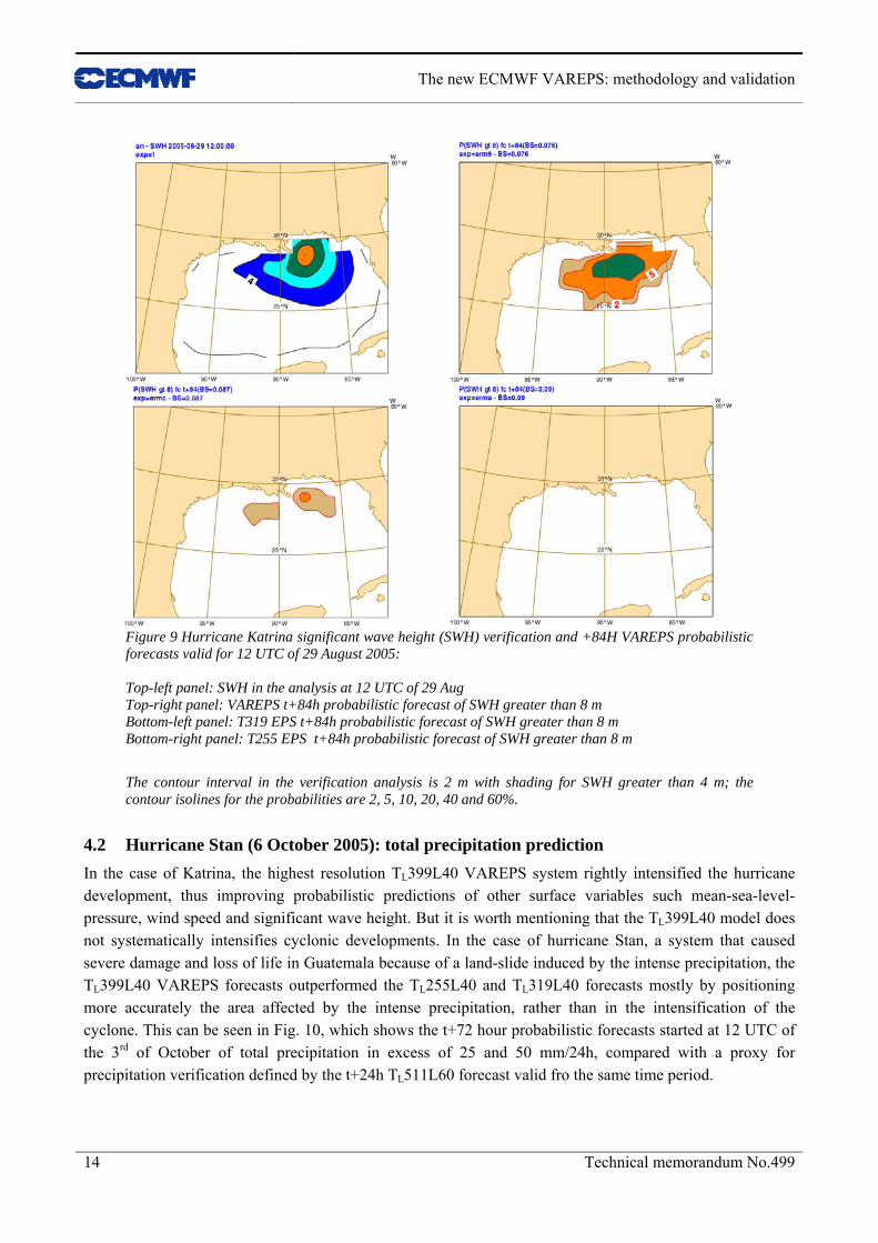
As a consequence of the more accurate development and intensification of the hurricane in each ensemble member, significant wave height probabilistic forecasts for the Gulf of Mexico are more accurate in the TL399L40 VAREPS. This can be seen, for example, by comparing the 84-hour probability forecasts of significant wave height in excess of 8 m (Fig. 9). The T255 system gives no probability of significant wave height exceeding 8 m and the T319 system gives a 2–5% probability, while the TL399L40 VAREPS system gives a 10–20% probability correctly located in the area where significant wave height exceeded 8m in the ECMWF operational analysis. Similar differences are detected by comparing probabilistic forecasts for earlier forecast ranges (not shown).



Figure 9 Hurricane Katrina significant wave height (SWH) verification and +84H VAREPS probabilistic forecasts valid for 12 UTC of 29 August 2005: Top-left panel: SWH in the analysis at 12 UTC of 29 Aug Top-right panel: VAREPS t+84h probabilistic forecast of SWH greater than 8 m Bottom-left panel: T319 EPS t+84h probabilistic forecast of SWH greater than 8 m Bottom-right panel: T255 EPS t+84h probabilistic forecast of SWH greater than 8 m

The contour interval in the verification analysis is 2 m with shading for SWH greater than 4 m; the contour isolines for the probabilities are 2, 5, 10, 20, 40 and 60%.

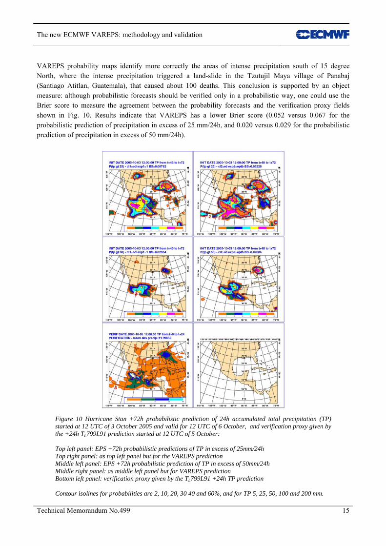
4.2 Hurricane Stan (6 October 2005): total precipitation prediction In the case of Katrina, the highest resolution TL399L40 VAREPS system rightly intensified the hurricane development, thus improving probabilistic predictions of other surface variables such mean-sea-level-pressure, wind speed and significant wave height. But it is worth mentioning that the TL399L40 model does not systematically intensifies cyclonic developments. In the case of hurricane Stan, a system that caused severe damage and loss of life in Guatemala because of a land-slide induced by the intense precipitation, the TL399L40 VAREPS forecasts outperformed the TL255L40 and TL319L40 forecasts mostly by positioning more accurately the area affected by the intense precipitation, rather than in the intensification of the cyclone. This can be seen in Fig. 10, which shows the t+72 hour probabilistic forecasts started at 12 UTC of the 3rd of October of total precipitation in excess of 25 and 50 mm/24h, compared with a proxy for precipitation verification defined by the t+24h TL511L60 forecast valid fro the same time period.



VAREPS probability maps identify more correctly the areas of intense precipitation south of 15 degree North, where the intense precipitation triggered a land-slide in the Tzutujil Maya village of Panabaj (Santiago Atitlan, Guatemala), that caused about 100 deaths. This conclusion is supported by an object measure: although probabilistic forecasts should be verified only in a probabilistic way, one could use the Brier score to measure the agreement between the probability forecasts and the verification proxy fields shown in Fig. 10. Results indicate that VAREPS has a lower Brier score (0.052 versus 0.067 for the probabilistic prediction of precipitation in excess of 25 mm/24h, and 0.020 versus 0.029 for the probabilistic prediction of precipitation in excess of 50 mm/24h).

Figure 10 Hurricane Stan +72h probabilistic prediction of 24h accumulated total precipitation (TP) started at 12 UTC of 3 October 2005 and valid for 12 UTC of 6 October, and verification proxy given by the +24h TL799L91 prediction started at 12 UTC of 5 October: Top left panel: EPS +72h probabilistic predictions of TP in excess of 25mm/24h Top right panel: as top left panel but for the VAREPS prediction Middle left panel: EPS +72h probabilistic prediction of TP in excess of 50mm/24h Middle right panel: as middle left panel but for VAREPS prediction Bottom left panel: verification proxy given by the TL799L91 +24h TP prediction Contour isolines for probabilities are 2, 10, 20, 30 40 and 60%, and for TP 5, 25, 50, 100 and 200 mm.



4.3 Flood of Firenze of 4 November 1966 (“L’Alluvione di Firenze del ‘66”): total precipitation prediction

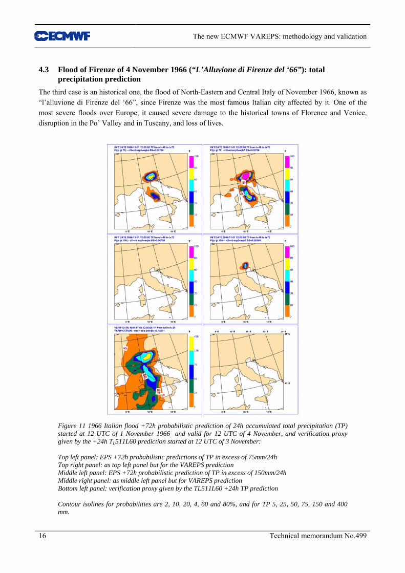
The third case is an historical one, the flood of North-Eastern and Central Italy of November 1966, known as “l’alluvione di Firenze del ‘66”, since Firenze was the most famous Italian city affected by it. One of the most severe floods over Europe, it caused severe damage to the historical towns of Florence and Venice, disruption in the Po’ Valley and in Tuscany, and loss of lives.

Figure 11 1966 Italian flood +72h probabilistic prediction of 24h accumulated total precipitation (TP) started at 12 UTC of 1 November 1966 and valid for 12 UTC of 4 November, and verification proxy given by the +24h TL511L60 prediction started at 12 UTC of 3 November: Top left panel: EPS +72h probabilistic predictions of TP in excess of 75mm/24h Top right panel: as top left panel but for the VAREPS prediction Middle left panel: EPS +72h probabilistic prediction of TP in excess of 150mm/24h Middle right panel: as middle left panel but for VAREPS prediction Bottom left panel: verification proxy given by the TL511L60 +24h TP prediction Contour isolines for probabilities are 2, 10, 20, 4, 60 and 80%, and for TP 5, 25, 50, 75, 150 and 400 mm.



Figure 11 shows the t+72 hour probabilistic prediction of total precipitation in excess of 75 and 150 mm/24h given by the T255 EPS and TL399 VAREPS systems valid for the 24-hour period starting at 12 UTC on 3 November. These probability maps can be compared with the proxy for precipitation verification given by a TL511L60 forecast started at 12 UTC on 3 November (Figure 8(e)). The proxy field represents rather accurately the overall pattern of the observed precipitation field, but underestimates the maximum values (Malguzzi et al 2006): during the verification period, maximum values of between 200 and 400 mm were observed in Tuscany, and values between 300 and 700 mm were observed in North-Eastern Italy.

Figure 11 shows that higher probability values are predicted by the TL399 VAREPS system both over Tuscany and North-Eastern Italy in the areas where intense precipitation was detected. It is interesting to point out that the TL399 VAREPS gives also a 40–60% probability that precipitation could exceed 150 mm over North-Eastern Italy, correctly indicating that North-Eastern Italy was going to be affected by the most intense rainfall.

4.4 Summer 2002: average temperature prediction over Europe Figure 3 discussed in Section 3.1 has shown that VAREPS probabilistic predictions of the 850 hPa temperature have, on average, a positive RPSS and a ROC area above 0.7 up to forecast day 13, thus suggesting that VAREPS probabilistic temperature predictions beyond forecast day 10 are skilful.

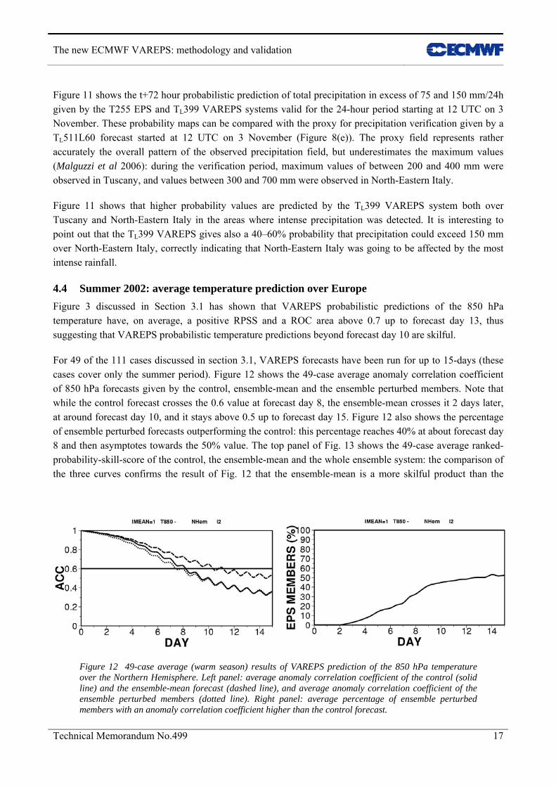
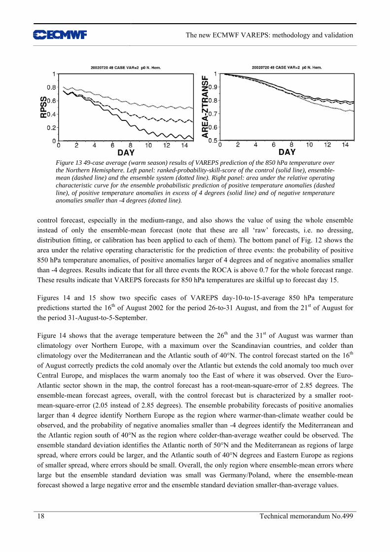
For 49 of the 111 cases discussed in section 3.1, VAREPS forecasts have been run for up to 15-days (these cases cover only the summer period). Figure 12 shows the 49-case average anomaly correlation coefficient of 850 hPa forecasts given by the control, ensemble-mean and the ensemble perturbed members. Note that while the control forecast crosses the 0.6 value at forecast day 8, the ensemble-mean crosses it 2 days later, at around forecast day 10, and it stays above 0.5 up to forecast day 15. Figure 12 also shows the percentage of ensemble perturbed forecasts outperforming the control: this percentage reaches 40% at about forecast day 8 and then asymptotes towards the 50% value. The top panel of Fig. 13 shows the 49-case average ranked-probability-skill-score of the control, the ensemble-mean and the whole ensemble system: the comparison of the three curves confirms the result of Fig. 12 that the ensemble-mean is a more skilful product than the

Figure 12 49-case average (warm season) results of VAREPS prediction of the 850 hPa temperature over the Northern Hemisphere. Left panel: average anomaly correlation coefficient of the control (solid line) and the ensemble-mean forecast (dashed line), and average anomaly correlation coefficient of the ensemble perturbed members (dotted line). Right panel: average percentage of ensemble perturbed members with an anomaly correlation coefficient higher than the control forecast.



Figure 13 49-case average (warm season) results of VAREPS prediction of the 850 hPa temperature over the Northern Hemisphere. Left panel: ranked-probability-skill-score of the control (solid line), ensemble-mean (dashed line) and the ensemble system (dotted line). Right panel: area under the relative operating characteristic curve for the ensemble probabilistic prediction of positive temperature anomalies (dashed line), of positive temperature anomalies in excess of 4 degrees (solid line) and of negative temperature anomalies smaller than -4 degrees (dotted line).

control forecast, especially in the medium-range, and also shows the value of using the whole ensemble instead of only the ensemble-mean forecast (note that these are all ‘raw’ forecasts, i.e. no dressing, distribution fitting, or calibration has been applied to each of them). The bottom panel of Fig. 12 shows the area under the relative operating characteristic for the prediction of three events: the probability of positive 850 hPa temperature anomalies, of positive anomalies larger of 4 degrees and of negative anomalies smaller than -4 degrees. Results indicate that for all three events the ROCA is above 0.7 for the whole forecast range. These results indicate that VAREPS forecasts for 850 hPa temperatures are skilful up to forecast day 15.

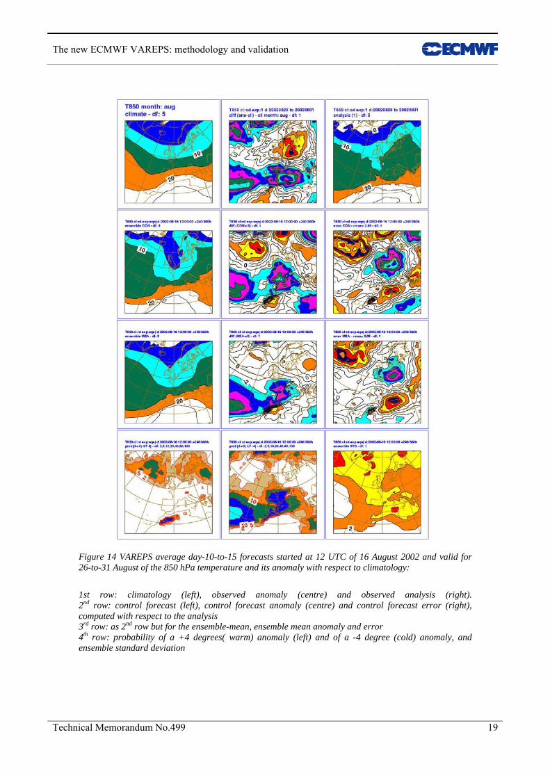
Figures 14 and 15 show two specific cases of VAREPS day-10-to-15-average 850 hPa temperature predictions started the 16th of August 2002 for the period 26-to-31 August, and from the 21st of August for the period 31-August-to-5-September.

Figure 14 shows that the average temperature between the 26th and the 31st of August was warmer than climatology over Northern Europe, with a maximum over the Scandinavian countries, and colder than climatology over the Mediterranean and the Atlantic south of 40°N. The control forecast started on the 16th of August correctly predicts the cold anomaly over the Atlantic but extends the cold anomaly too much over Central Europe, and misplaces the warm anomaly too the East of where it was observed. Over the Euro-Atlantic sector shown in the map, the control forecast has a root-mean-square-error of 2.85 degrees. The ensemble-mean forecast agrees, overall, with the control forecast but is characterized by a smaller root-mean-square-error (2.05 instead of 2.85 degrees). The ensemble probability forecasts of positive anomalies larger than 4 degree identify Northern Europe as the region where warmer-than-climate weather could be observed, and the probability of negative anomalies smaller than -4 degrees identify the Mediterranean and the Atlantic region south of 40°N as the region where colder-than-average weather could be observed. The ensemble standard deviation identifies the Atlantic north of 50°N and the Mediterranean as regions of large spread, where errors could be larger, and the Atlantic south of 40°N degrees and Eastern Europe as regions of smaller spread, where errors should be small. Overall, the only region where ensemble-mean errors where large but the ensemble standard deviation was small was Germany/Poland, where the ensemble-mean forecast showed a large negative error and the ensemble standard deviation smaller-than-average values.



Figure 14 VAREPS average day-10-to-15 forecasts started at 12 UTC of 16 August 2002 and valid for 26-to-31 August of the 850 hPa temperature and its anomaly with respect to climatology:

1st row: climatology (left), observed anomaly (centre) and observed analysis (right). 2nd row: control forecast (left), control forecast anomaly (centre) and control forecast error (right), computed with respect to the analysis 3rd row: as 2nd row but for the ensemble-mean, ensemble mean anomaly and error 4th row: probability of a +4 degrees( warm) anomaly (left) and of a -4 degree (cold) anomaly, and ensemble standard deviation



Figure 15 As Fig. 12 but for the VAREPS average day-10-to-15 forecasts started at 12 UTC of 21 August 2002 and valid for 31 August to 5 September of the 850 hPa temperature and its anomaly with respect to climatology:

Figure 15 shows that the average temperature between the 31st of August and the 5th of September was warmer than climatology over North-Eastern Europe, with a maximum over Finland, and over Northern Africa, and colder than climatology over the Mediterranean. The control forecast started on the 21st of August correctly predicts the warm anomaly over North-Eastern Europe and Northern Africa and the cold anomaly over the Mediterranean, but it wrongly predicts a warm anomaly south of the British Isles. Over the Euro-Atlantic sector shown in the map, the control forecast has a root-mean-square-error of 1.89 degrees. The ensemble-mean forecast agrees, overall, with the control forecast but does not show a warm anomaly



south of the British Isles as the control does, and is characterized by a smaller root-mean-square-error (1.46 instead of 1.89 degrees). The ensemble probability forecasts of positive anomalies larger than 4 degree identify North-Eastern Europe and Northern Africa as the regions where warmer-than-climate weather could be observed, and the probability of negative anomalies smaller than -4 degrees also gives a small probability that the Mediterranean could be a region where colder-than-average weather could be observed. The ensemble standard deviation identifies only North-Eastern Atlantic as the region of large spread, where errors could be larger-than-average. Compared to the previous case, the ensemble standard deviation is smaller over the whole Euro-Atlantic region, correctly identifying this as a more predictable case than the previous one.

These two cases indicate that the combined use of day-10-to-15 control and ensemble-mean forecast, probability maps and ensemble standard deviation could provide some valuable and skilful predictions of regions of warm/cold anomalies with respect to the climate, and of regions where forecasts errors could be larger/smaller than average.

5. Planned VAREPS implementation schedule, and future changes of the ECMWF probabilistic system

The ECMWF Variable Resolution Ensemble Prediction System (VAREPS) has been designed to increase the ensemble resolution in the early forecast range and to extend the forecast range covered by the ensemble system initially to 15 days and eventually to 32 days, following the planned merging of the ensemble and the monthly operational system.

In this work, VAREPS forecasts, performed with resolution TL399L40 between forecast days 0-7 and TL255L40 between forecast days 7-15, have been assessed and compared to two constant resolution systems, a TL255L40 and a TL319L40 ones (this latter one requires similar computing resources to VAREPS).

Average results based on 111-cases have indicated that VAREPS is more skilful than a T255 EPS, with differences statistically significant in the early forecast range (say up to forecast day 7). Although on average these differences are small, the analysis of some cases characterized by severe weather developments have indicated that the differences can be very large, and lead to substantial improvements, especially in the prediction of surface weather variables, such as mean-sea-level-pressure, wind speed, significant wave height and total precipitation. Average results have also shown that VAREPS forecasts can provide some skilful forecasts of average quantities, such as 850 hPa temperature, beyond forecast day 10. Finally, the comparison of VAREPS forecasts with forecasts generated using a constant-resolution T319 EPS, which requires the same amount of computing resources as VAREPS, have indicated that VAREPS is a better system, since it provides significantly better forecasts in the early forecast range without loosing accuracy in the long forecast range.

From an operational point of view, on the 1st of February 2006 ECMWF increased the resolution of the operational Ensemble Prediction System (EPS) from TL255L40(d0-10) to TL399L62(day 0–10): this upgrade was the first of a three-phase upgrading process that will lead to the implementation of the ECMWF Variable Resolution Ensemble Prediction System (VAREPS).

The second of this three-phase upgrading process, planned for the second half of 2006, will lead to the extension of the 00 and 12 UTC ensemble systems to 15 days using the VAREPS approach, with a



TL399L62 resolution up to forecast day 10 and a TL255L62 resolution between forecast day 10 and 15. Thus, in the planned operational VAREPS the resolution will be truncated at forecast day 10 instead of 7 (leg-2 will still start 24-hour before the truncation period to reduce the impact of truncation on the forecast fields of variables such as total precipitation). The decision to apply the truncation at forecast day 10 instead of 7 was a technical one, designed to address some users’ concerns and simplify their use of ensemble forecasts. In fact, a day-10 truncation means that only users who want to use ensemble forecasts beyond forecast day 10 have to modify their programmes to generate their products (see Appendix A for more details), while users who decided to limit their use of ensemble products to forecast day 10 do not need to apply any technical change to generate their ensemble products. It is worth mentioning that, again following a users’ request, VAREPS will also include two other constant-resolution forecasts for calibration/validation purposes: a 15-day TL399L62 forecast and a 15-day TL255L62 forecast.

The detailed configuration of VAREPS that will be implemented in the third phase is still under discussion, but its aim is to extend VAREPS to one month, with a TL255L62 atmospheric resolution and ocean coupling most likely introduced at day 10.

VAREPS will help ECMWF to further increase the value of its probabilistic forecasting system, and deliver to ECMWF users more accurate predictions of small-scale, severe weather events in the early forecast range and skilful probabilistic predictions of larger scale features in the medium forecast range.

Acknowledgements

The development, operational implementation, and continuous improvement of the ECMWF Ensemble Prediction System would not have been possible without the contribution of many staff members and consultants: their work is acknowledged. Roberto Buizza would also like to thank Dr. Laurie Wilson, of MSC Canada, for his advice and help in the revision of the computation of the area under the relative operative characteristic curve.



Appendix A. Computation of accumulated fields across the truncation forecast step

Figure 1 shows a schematic of the two legs of each VAREPS forecast. In the Field Data Base (FDB) and in the Meteorological Archival and Retrieval System (MARS), leg-1 data are written in stream = ENFO, while leg-2 data are written in the overlap stream EFOV between forecast day 9 and 10, and in stream ENFO only after day 10. Note that the leg-1 accumulated field at the truncation step tTR interpolated on the TL255 reduced Gaussian grid, AFvar(tTR), is also archived in stream EFOV.

Let us introduce the following variables:

• t: forecast step (0≤t≤360)

• AF(t): the accumulated field (accumulated from the start of the forecast) in the FDB/MARS stream ENFO

• INTERP255[AF(t)]: the interpolation of AF(t) on the TL255 reduced Gaussian grid

• INTERPUG[AF(t)]: the interpolation of AF(t) on the user’s grid

• AF255(t): the AF(t) field interpolated on the TL255 reduced Gaussian grid:

AF255(t) = INTERP255[AF(t)]

• AFUG(t): the AF(t) field interpolated on the user’s grid (e.g. the TL255 reduced Gaussian grid, or a regular lat/long grid):

AFUG(t) = INTERPUG[AF(t)]

• AFvar(tTR): the leg-1 accumulated field interpolated on the TL255 Gaussian grid retrieved from stream = EFOV

• AFUG(t1,t2): the field accumulated between forecast steps t1 and t2 on the user’s grid

Let us compute AFUG(t1,t2) for all forecast intervals (t1,t2).

If the forecast interval (t1,t2) includes the truncation step tTR, t1≤tTR≤t2 and the user’s grid is different from the TL255 reduced Gaussian grid, the fields archived in the overlap stream should be used to compute correctly AFUG(t1,t2), as discussed below. This procedure is necessary because the leg-2 day-10 forecasts (i.e. after 24-hour integration, see Figure 2) of the accumulated fields are re-set to be equal to the TL399L62 ones interpolated on the TL255 reduced Gaussian grid.



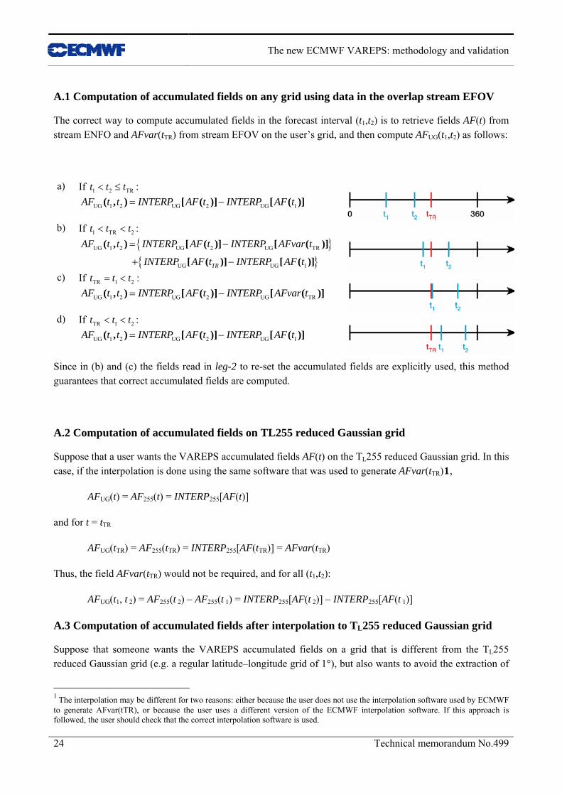
A.1 Computation of accumulated fields on any grid using data in the overlap stream EFOV

The correct way to compute accumulated fields in the forecast interval (t1,t2) is to retrieve fields AF(t) from stream ENFO and AFvar(tTR) from stream EFOV on the user’s grid, and then compute AFUG(t1,t2) as follows:

a) If : 1 2 TRt t t< ≤

UG 1 2 UG 2 UG 1( , ) [ ( )] [ ( )]AF t t INTERP AF t INTERP AF t= −

b) If t t : 1 TR 2t< <

{ }{ }

UG 1 2 UG 2 UG TR

UG UG 1

( , ) [ ( )] [ ( )]

[ ( )] [ ( )]TR

AF t t INTERP AF t INTERP AFvar t

INTERP AF t INTERP AF t

= −

+ −

c) If : TR 1 2t t t= <

UG 1 2 UG 2 UG TR( , ) [ ( )] [ ( )]AF t t INTERP AF t INTERP AFvar t= −

d) If : TR 1 2t t< < t

UG 1 2 UG 2 UG 1( , ) [ ( )] [ ( )]AF t t INTERP AF t INTERP AF t= −

Since in (b) and (c) the fields read in leg-2 to re-set the accumulated fields are explicitly used, this method guarantees that correct accumulated fields are computed.

A.2 Computation of accumulated fields on TL255 reduced Gaussian grid

Suppose that a user wants the VAREPS accumulated fields AF(t) on the TL255 reduced Gaussian grid. In this case, if the interpolation is done using the same software that was used to generate AFvar(tTR)1,

AFUG(t) = AF255(t) = INTERP255[AF(t)]

and for t = tTR

AFUG(tTR) = AF255(tTR) = INTERP255[AF(tTR)] = AFvar(tTR)

Thus, the field AFvar(tTR) would not be required, and for all (t1,t2):

AFUG(t1, t 2) = AF255(t 2) – AF255(t 1) = INTERP255[AF(t 2)] – INTERP255[AF(t 1)]

A.3 Computation of accumulated fields after interpolation to TL255 reduced Gaussian grid

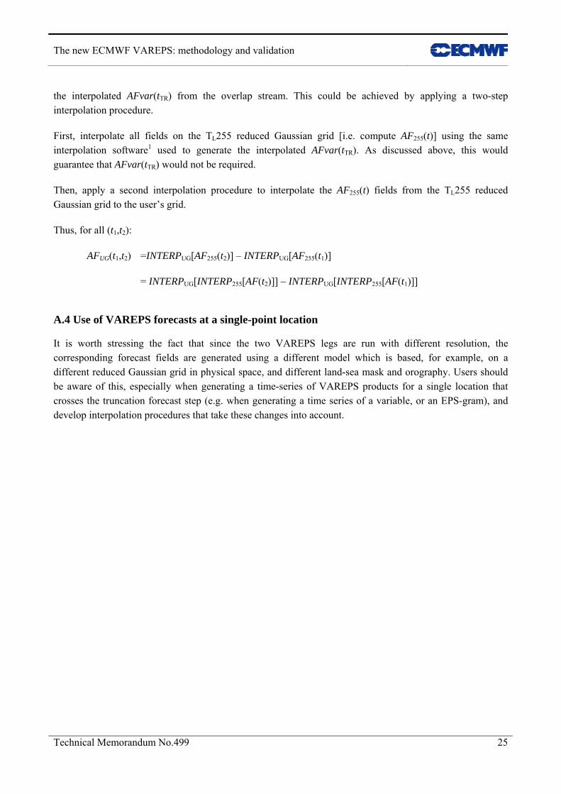
Suppose that someone wants the VAREPS accumulated fields on a grid that is different from the TL255 reduced Gaussian grid (e.g. a regular latitude–longitude grid of 1°), but also wants to avoid the extraction of

1 The interpolation may be different for two reasons: either because the user does not use the interpolation software used by ECMWF to generate AFvar(tTR), or because the user uses a different version of the ECMWF interpolation software. If this approach is followed, the user should check that the correct interpolation software is used.



the interpolated AFvar(tTR) from the overlap stream. This could be achieved by applying a two-step interpolation procedure.

First, interpolate all fields on the TL255 reduced Gaussian grid [i.e. compute AF255(t)] using the same interpolation software1 used to generate the interpolated AFvar(tTR). As discussed above, this would guarantee that AFvar(tTR) would not be required.

Then, apply a second interpolation procedure to interpolate the AF255(t) fields from the TL255 reduced Gaussian grid to the user’s grid.

Thus, for all (t1,t2):

AFUG(t1,t2) =INTERPUG[AF255(t2)] – INTERPUG[AF255(t1)]

= INTERPUG[INTERP255[AF(t2)]] – INTERPUG[INTERP255[AF(t1)]]

A.4 Use of VAREPS forecasts at a single-point location

It is worth stressing the fact that since the two VAREPS legs are run with different resolution, the corresponding forecast fields are generated using a different model which is based, for example, on a different reduced Gaussian grid in physical space, and different land-sea mask and orography. Users should be aware of this, especially when generating a time-series of VAREPS products for a single location that crosses the truncation forecast step (e.g. when generating a time series of a variable, or an EPS-gram), and develop interpolation procedures that take these changes into account.



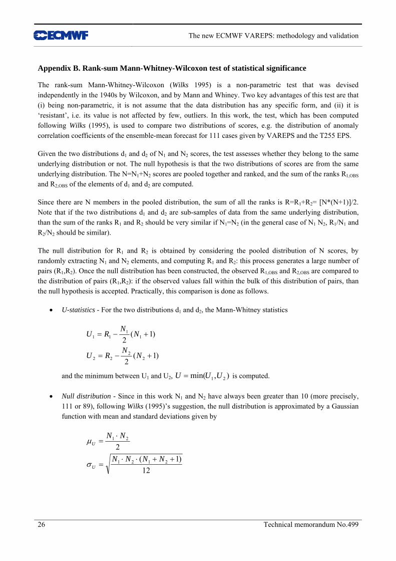
Appendix B. Rank-sum Mann-Whitney-Wilcoxon test of statistical significance

The rank-sum Mann-Whitney-Wilcoxon (Wilks 1995) is a non-parametric test that was devised independently in the 1940s by Wilcoxon, and by Mann and Whiney. Two key advantages of this test are that (i) being non-parametric, it is not assume that the data distribution has any specific form, and (ii) it is ‘resistant’, i.e. its value is not affected by few, outliers. In this work, the test, which has been computed following Wilks (1995), is used to compare two distributions of scores, e.g. the distribution of anomaly correlation coefficients of the ensemble-mean forecast for 111 cases given by VAREPS and the T255 EPS.

Given the two distributions d1 and d2 of N1 and N2 scores, the test assesses whether they belong to the same underlying distribution or not. The null hypothesis is that the two distributions of scores are from the same underlying distribution. The N=N1+N2 scores are pooled together and ranked, and the sum of the ranks R1,OBS and R2,OBS of the elements of d1 and d2 are computed.

Since there are N members in the pooled distribution, the sum of all the ranks is R=R1+R2= [N*(N+1)]/2. Note that if the two distributions d1 and d2 are sub-samples of data from the same underlying distribution, than the sum of the ranks R1 and R2 should be very similar if N1=N2 (in the general case of N1 N2, R1/N1 and R2/N2 should be similar).

The null distribution for R1 and R2 is obtained by considering the pooled distribution of N scores, by randomly extracting N1 and N2 elements, and computing R1 and R2: this process generates a large number of pairs (R1,R2). Once the null distribution has been constructed, the observed R1,OBS and R2,OBS are compared to the distribution of pairs (R1,R2): if the observed values fall within the bulk of this distribution of pairs, than the null hypothesis is accepted. Practically, this comparison is done as follows.

• U-statistics - For the two distributions d1 and d2, the Mann-Whitney statistics

)1(

2

)1(2

22

22

11

11

+−=

+−=

NN

RU

NN

RU

and the minimum between U1 and U2, ),min( 21 UUU = is computed.

• Null distribution - Since in this work N1 and N2 have always been greater than 10 (more precisely, 111 or 89), following Wilks (1995)’s suggestion, the null distribution is approximated by a Gaussian function with mean and standard deviations given by

12)1(

2

2121

21

++⋅⋅=

⋅=

NNNN

NN

U

U

σ

μ



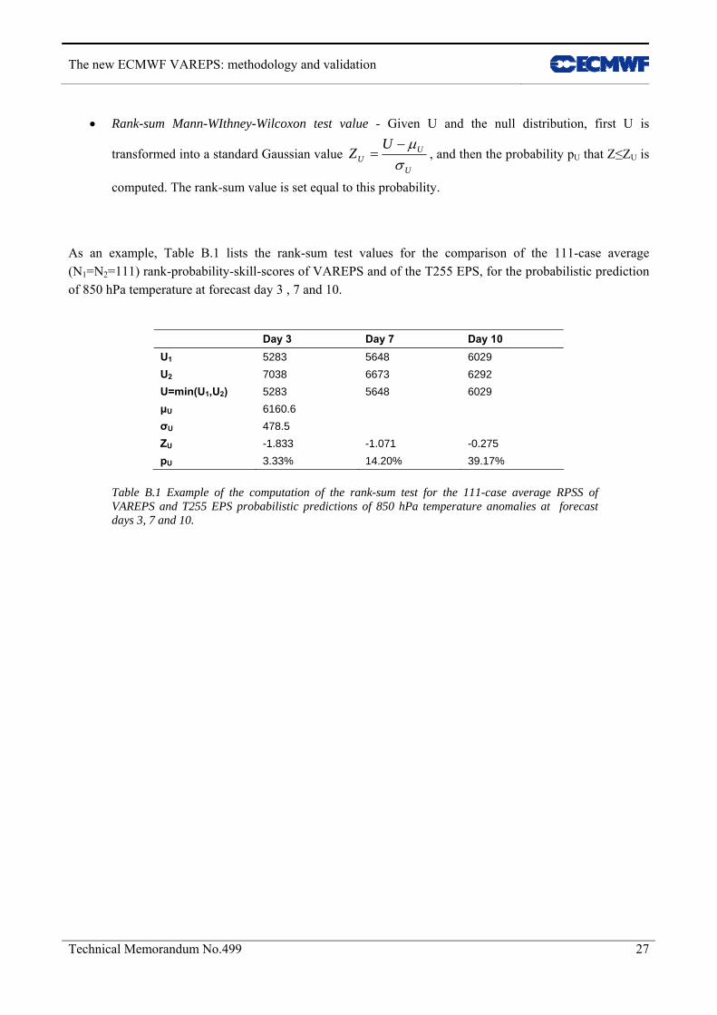
• Rank-sum Mann-WIthney-Wilcoxon test value - Given U and the null distribution, first U is

transformed into a standard Gaussian value U

UU

UZ

σμ−

= , and then the probability pU that Z≤ZU is

computed. The rank-sum value is set equal to this probability.

As an example, Table B.1 lists the rank-sum test values for the comparison of the 111-case average (N1=N2=111) rank-probability-skill-scores of VAREPS and of the T255 EPS, for the probabilistic prediction of 850 hPa temperature at forecast day 3 , 7 and 10.

Day 3 Day 7 Day 10 U1 5283 5648 6029 U2 7038 6673 6292 U=min(U1,U2) 5283 5648 6029 μU 6160.6 σU 478.5 ZU -1.833 -1.071 -0.275 pU 3.33% 14.20% 39.17%

Table B.1 Example of the computation of the rank-sum test for the 111-case average RPSS of

VAREPS and T255 EPS probabilistic predictions of 850 hPa temperature anomalies at forecast days 3, 7 and 10.



Appendix C. Computation of the area under the Relative Operating Characteristics in Z-transformed coordinates

Given a dichotomous event(e.g. the prediction of positive 850 hPa temperature anomaly), the area under the relative operating characteristic curve (ROCA) measures the capability of a forecasting system to discriminate between hit and false alarms (Mason 1982).

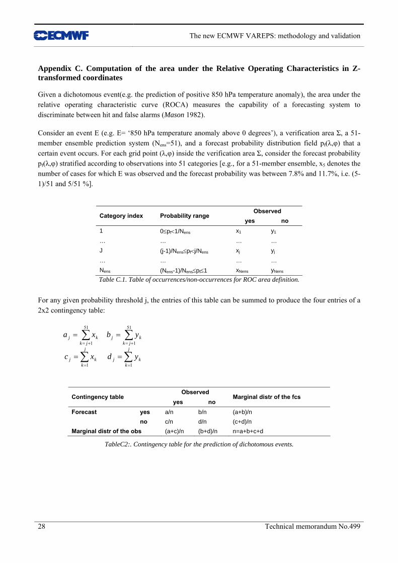
Consider an event E (e.g. E= ‘850 hPa temperature anomaly above 0 degrees’), a verification area Σ, a 51-member ensemble prediction system (Nens=51), and a forecast probability distribution field pf(λ,φ) that a certain event occurs. For each grid point (λ,φ) inside the verification area Σ, consider the forecast probability pf(λ,φ) stratified according to observations into 51 categories [e.g., for a 51-member ensemble, x5 denotes the number of cases for which E was observed and the forecast probability was between 7.8% and 11.7%, i.e. (5-1)/51 and 5/51 %].

Observed

Category index Probability range yes no

1 0≤pf<1/Nens x1 y1

… … … … J (j-1)/Nens≤pf<j/Nens xj yj

… … … … Nens (Nens-1)/Nens≤pf≤1 xNens yNens

Table C.1. Table of occurrences/non-occurrences for ROC area definition.

For any given probability threshold j, the entries of this table can be summed to produce the four entries of a 2x2 contingency table:

∑∑

∑∑

==

+=+=

==

==

j

kkj

j

kkj

jkkj

jkkj

ydxc

ybxa

11

51

1

51

1

Observed

Contingency table yes no

Marginal distr of the fcs

yes a/n b/n (a+b)/n Forecast no c/n d/n (c+d)/n

Marginal distr of the obs (a+c)/n (b+d)/n n=a+b+c+d

TableC2:. Contingency table for the prediction of dichotomous events.



From each of the j-th contingency tables, the probability of detection PODj and the probability of false detection PFDj can be computed:

)(

)(

jj

jj

jj

jj

dbb

PFD

caa

POD

+=

+=

The 51 pairs (PFDj,PODj) can be plotted one against the other on a graph: the result is a curve called the relative operating characteristic (ROC) curve.

As suggested by Wilson (2000), and following Swets (1986), the area under the ROC curve is computed in terms of the standard normal deviates of the hit and false alarm rates:

First, each pair is tranformed into a pair of standard normal deviates , where

Z0

),( jj PFDPOD )1,0( jj ZZ

j and Z1j are the standard normal deviates that correpond to the cumulative probabilities PODj and PFDj:

∫

∫

∞−

−

∞−

−

=

=

j

j

Zx

j

Zx

j

dxePFD

dxePOD

1

0

2

2

21

21

π

π

Then, once all pairs have been computed, the straight line )1,0( jj ZZ bzmy +⋅= that best fits them is

computed using the ‘least-squares’ method, and the distance between the best-fit curve bzmy +⋅= and the origin (0,0) is computed:

12 +

=m

bD

Finally, the area under the ROC curve, ROCA, is calculated as the cumulative probability that corresponds to D:

∫∞−

−=D

x dxeROCA2

21π



References

Barkmeijer, J., R. Buizza & T.N. Palmer, 1999: 3D-Var Hessian singular vectors and their potential use in the ECMWF Ensemble Prediction System. Q. J. R. Meteorol. Soc., 125, 2333–2351.

Barkmeijer, J., R. Buizza, T.N. Palmer, K. Puri & J.-F. Mahfouf, 2001: Tropical singular vectors computed with linearized diabatic physics. Q. J. R. Meteorol. Soc., 127, 685–708 (also available as ECMWF Technical Memo. No. 297).

Brier, G. W., 1950: Verification of forecasts expressed in terms of probability. Mon. Wea. Rev., 78, 1-3.

Buizza, R., & T.N. Palmer, 1995: The singular-vector structure of the atmospheric global circulation. J. Atmos. Sci., 52, 1434-1456.

Buizza, R., & T.N. Palmer, 1998: Impact of ensemble size on ensemble prediction. Mon. Wea. Rev., 126, 2503-2518.

Buizza, R., T. Petroliagis, T. N. Palmer, J. Barkmeijer, M. Hamrud, A. Hollingsworth, A. Simmons, & N. Wedi, 1998: Impact of model resolution and ensemble size on the performance of an ensemble prediction system. Q. J. R. Meteorol. Soc., 124, 1935-1960.

Buizza, R., M. Miller, & T. N. Palmer, 1999: Stochastic representation of model uncertainties in the ECMWF ensemble prediction system. Q. J. R. Meteorol. Soc., 125, 2887-2908.

Buizza, R., D. S. Richardson, & T. N. Palmer, 2003: Benefits of increased resolution in the ECMWF ensemble system and comparison with poor-man’s ensembles. Q. J. R. Meteorol. Soc., 129, 1269-1288.

Ehrendorfer, M. & A. Beck, 2003: Singular vector-based multivariate sampling in ensemble prediction. ECMWF Technical Memo. No. 416.

Janssen P., J.-R Bidlot, S. Abdalla & H. Hersbach, 2005: Progress in ocean wave forecasting at ECMWF. ECMWF Technical Memo. No. 478, available from ECMWF, Shinfield Park, Reading RG2-9AX, UK.

Malguzzi, P, G. Grossi, A. Buzzi, R. Ranzi,, & R. Buizza, 2006: The 1966 'century' flood in Italy: a meteorological-hydrological revisitation. J. Geoph. Res., under revision.

Molteni, F., R. Buizza, T. N. Palmer, & T. Petroliagis, 1996: The ECMWF ensemble prediction system: methodology and validation. Q. J. R. Meteorol. Soc., 122, 73-119.

Palmer, T. N., F. Molteni, R. Mureau, & R. Buizza, 1993: Ensemble prediction. ECMWF Seminar Proceedings ‘Validation of models over Europe: Vol. I’, available from ECMWF, Shinfield Park, Reading RG2-9AX, UK.

Pellerin, G., Lefaivre, L., Houtekamer, P., and Girard, C., 2003: Increasing the horizontal resolution of ensemble forecasts at CMC. Non-linear Processes in Geophysics, 10, 463-488.



Saetra, Ø. & J.-R Bidlot, 2004: On the potential benefit of using probabilistic forecast for waves and marine winds based on the ECMWF ensemble prediction system. Wea. Forecasting, 19, 673-689.

Stanski, H. R., L. J. Wilson, & W. R. Burrows, 1989. Survey of common verification methods in meteorology. World Weather Watch Technical Report No. 8, WMO/TD. No. 358, World Meteorological Organization. 114 pp.

Swets, J. A., 1986: Form of empirical ROCs in discrimination and diagnostic tasks: Implications for theory and measurement of performance. Psycol. Bull., 99, 181-198.

Talagrand, O., R. Vautard, & B. Strauss, 1997: Evaluation of probabilistic prediction systems. Proceedings of the ECMWF Workshop on Predictability, 20-22 October 1997, ECMWF, Shinfield Park, Reading RG2-9AX, 1-26.

Wilks, D. S., 1995: Statistical methods in the atmospheric sciences. Academic Press, Inc., San Diego, pp. 467 (ISBN 0-12-751965-3).

Wilson, L. J., 2000: Comments on “Probabilistic predictions of precipitations using the ECMWF ensemble prediction system”. Weather and Forecasting, 15, 361-364.

Toth, Z., & Kalnay, E., 1997: Ensemble Forecasting at NCEP and the breeding method. Mon. Wea. Rev., 125, 3297-3319.

Documents

The new ECMWF Variable Resolution Ensemble Prediction ... · 499 The new ECMWF Variable Resolution Ensemble Prediction System (VAREPS): methodology and validation Roberto Buizza,