Embed Size (px)
Citation preview

The nonperturbative functional renormalization group and its applications
N. Dupuisa, L. Canetb, A. Eichhornc,d, W. Metznere, J. M. Pawlowskid,f, M. Tissiera, N. Wscheborg
aSorbonne Universite, CNRS, Laboratoire de Physique Theorique de la Matiere Condensee, LPTMC, F-75005 Paris, FrancebUniversite Grenoble Alpes and CNRS, Laboratoire de Physique et Modelisation des Milieux Condenses, LPMMC, 38000 Grenoble, France
cCP3-Origins, University of Southern Denmark, Campusvej 55, DK-5230 Odense M, DenmarkdInstitut fur Theoretische Physik, Universitat Heidelberg, Philosophenweg 16, 69120 Heidelberg, Germany
eMax-Planck-Institute for Solid State Research, Heisenbergstraße 1, D-70569 Stuttgart, GermanyfExtreMe Matter Institute EMMI, GSI, Planckstr. 1, D-64291 Darmstadt, Germany
gInstituto de Fısica, Facultad de Ingenierıa, Universidad de la Republica, J.H.y Reissig 565, 11000 Montevideo, Uruguay
Abstract
The renormalization group plays an essential role in many areas of physics, both conceptually and as a practical toolto determine the long-distance low-energy properties of many systems on the one hand and on the other hand searchfor viable ultraviolet completions in fundamental physics. It provides us with a natural framework to study theoreticalmodels where degrees of freedom are correlated over long distances and that may exhibit very distinct behavior on dif-ferent energy scales. The nonperturbative functional renormalization-group (FRG) approach is a modern implementa-tion of Wilson’s RG, which allows one to set up nonperturbative approximation schemes that go beyond the standardperturbative RG approaches. The FRG is based on an exact functional flow equation of a coarse-grained effectiveaction (or Gibbs free energy in the language of statistical mechanics). We review the main approximation schemesthat are commonly used to solve this flow equation and discuss applications in equilibrium and out-of-equilibriumstatistical physics, quantum many-particle systems, high-energy physics and quantum gravity.
Contents
1 Introduction 31.1 Wilson’s renormalization group . . . . . . . . . . . . . . . . . . . . . . . . . . . . . . . . . . . . . . 41.2 The functional renormalization group . . . . . . . . . . . . . . . . . . . . . . . . . . . . . . . . . . 41.3 Scope of the review . . . . . . . . . . . . . . . . . . . . . . . . . . . . . . . . . . . . . . . . . . . . 5
2 The FRG in a nutshell 62.1 The scale-dependent effective action . . . . . . . . . . . . . . . . . . . . . . . . . . . . . . . . . . . 6
2.1.1 The regulator function Rk . . . . . . . . . . . . . . . . . . . . . . . . . . . . . . . . . . . . . 72.1.2 General properties of the effective action Γk . . . . . . . . . . . . . . . . . . . . . . . . . . . 7
2.2 The exact flow equation . . . . . . . . . . . . . . . . . . . . . . . . . . . . . . . . . . . . . . . . . . 82.3 The derivative expansion (DE) . . . . . . . . . . . . . . . . . . . . . . . . . . . . . . . . . . . . . . 9
2.3.1 Local-potential approximation: LPA and LPA′ . . . . . . . . . . . . . . . . . . . . . . . . . 102.3.2 Second order of the DE . . . . . . . . . . . . . . . . . . . . . . . . . . . . . . . . . . . . . . 112.3.3 Validity of the DE . . . . . . . . . . . . . . . . . . . . . . . . . . . . . . . . . . . . . . . . 132.3.4 Further results obtained from the DE . . . . . . . . . . . . . . . . . . . . . . . . . . . . . . . 13
2.4 Computing momentum-dependent correlation functions . . . . . . . . . . . . . . . . . . . . . . . . . 142.5 Lattice models and realistic microscopic actions . . . . . . . . . . . . . . . . . . . . . . . . . . . . . 152.6 Quantum models . . . . . . . . . . . . . . . . . . . . . . . . . . . . . . . . . . . . . . . . . . . . . 15
3 Statistical mechanics 153.1 Why and when is the FRG useful? . . . . . . . . . . . . . . . . . . . . . . . . . . . . . . . . . . . . 153.2 Equilibrium statistical mechanics . . . . . . . . . . . . . . . . . . . . . . . . . . . . . . . . . . . . . 16
3.2.1 Frustrated magnets as an example . . . . . . . . . . . . . . . . . . . . . . . . . . . . . . . . 16
Preprint submitted to Elsevier May 10, 2021
arX
iv:2
006.
0485
3v3
[co
nd-m
at.s
tat-
mec
h] 7
May
202
1

3.2.2 Critical phenomena and universal long distance regime . . . . . . . . . . . . . . . . . . . . . 193.2.3 Nonuniversal properties . . . . . . . . . . . . . . . . . . . . . . . . . . . . . . . . . . . . . 193.2.4 Conformal invariance and c-theorem . . . . . . . . . . . . . . . . . . . . . . . . . . . . . . . 20
3.3 Disordered systems . . . . . . . . . . . . . . . . . . . . . . . . . . . . . . . . . . . . . . . . . . . . 203.3.1 Replica formalism and FRG . . . . . . . . . . . . . . . . . . . . . . . . . . . . . . . . . . . 203.3.2 The Random Field Ising Model . . . . . . . . . . . . . . . . . . . . . . . . . . . . . . . . . 213.3.3 Other disordered systems . . . . . . . . . . . . . . . . . . . . . . . . . . . . . . . . . . . . . 23
3.4 Classical non-equilibrium systems and FRG . . . . . . . . . . . . . . . . . . . . . . . . . . . . . . . 233.4.1 Langevin stochastic dynamics . . . . . . . . . . . . . . . . . . . . . . . . . . . . . . . . . . 243.4.2 Master equations: reaction-diffusion processes . . . . . . . . . . . . . . . . . . . . . . . . . 303.4.3 Non-equilibrium quantum systems . . . . . . . . . . . . . . . . . . . . . . . . . . . . . . . . 32
4 Quantum many-particle systems 334.1 Bosons . . . . . . . . . . . . . . . . . . . . . . . . . . . . . . . . . . . . . . . . . . . . . . . . . . . 33
4.1.1 Superfluidity in a dilute Bose gas . . . . . . . . . . . . . . . . . . . . . . . . . . . . . . . . 334.1.2 Superfluid to Mott-insulator transition . . . . . . . . . . . . . . . . . . . . . . . . . . . . . . 344.1.3 Relativistic bosons and quantum O(N) model . . . . . . . . . . . . . . . . . . . . . . . . . . 35
4.2 Fermions . . . . . . . . . . . . . . . . . . . . . . . . . . . . . . . . . . . . . . . . . . . . . . . . . 364.2.1 Fermion flow equation . . . . . . . . . . . . . . . . . . . . . . . . . . . . . . . . . . . . . . 374.2.2 Competing instabilities . . . . . . . . . . . . . . . . . . . . . . . . . . . . . . . . . . . . . . 384.2.3 Spontaneous symmetry breaking . . . . . . . . . . . . . . . . . . . . . . . . . . . . . . . . . 414.2.4 Quantum transport . . . . . . . . . . . . . . . . . . . . . . . . . . . . . . . . . . . . . . . . 424.2.5 Leap to strong coupling . . . . . . . . . . . . . . . . . . . . . . . . . . . . . . . . . . . . . 434.2.6 Omissions . . . . . . . . . . . . . . . . . . . . . . . . . . . . . . . . . . . . . . . . . . . . . 44
5 High-energy physics 455.1 Introduction: High-energy physics . . . . . . . . . . . . . . . . . . . . . . . . . . . . . . . . . . . . 455.2 The functional renormalization group for gauge theories . . . . . . . . . . . . . . . . . . . . . . . . 45
5.2.1 Gauge-fixed flows and modified Slavnov-Taylor identities . . . . . . . . . . . . . . . . . . . 465.2.2 Gauge invariance, locality & confinement . . . . . . . . . . . . . . . . . . . . . . . . . . . . 505.2.3 Gauge-invariant flows & the quest for simplicity . . . . . . . . . . . . . . . . . . . . . . . . 52
5.3 QCD . . . . . . . . . . . . . . . . . . . . . . . . . . . . . . . . . . . . . . . . . . . . . . . . . . . . 535.3.1 Confinement and the flow of composite operators . . . . . . . . . . . . . . . . . . . . . . . . 545.3.2 Chiral symmetry breaking . . . . . . . . . . . . . . . . . . . . . . . . . . . . . . . . . . . . 565.3.3 Vacuum QCD and hadronic bound states . . . . . . . . . . . . . . . . . . . . . . . . . . . . 57
5.4 Phase structure and dynamics of QCD . . . . . . . . . . . . . . . . . . . . . . . . . . . . . . . . . . 605.4.1 The unreasonable effectiveness of low-energy effective theories . . . . . . . . . . . . . . . . 605.4.2 The phase structure of QCD from low-energy effective models . . . . . . . . . . . . . . . . . 615.4.3 Towards the QCD phase structure from first principles . . . . . . . . . . . . . . . . . . . . . 63
5.5 Electroweak phase transition, BSM physics & Supersymmetry . . . . . . . . . . . . . . . . . . . . . 645.6 Summary . . . . . . . . . . . . . . . . . . . . . . . . . . . . . . . . . . . . . . . . . . . . . . . . . 65
6 Gravity 656.1 Introduction: Quantum gravity - why and what? . . . . . . . . . . . . . . . . . . . . . . . . . . . . . 656.2 Path integral for quantum gravity and asymptotic safety . . . . . . . . . . . . . . . . . . . . . . . . . 676.3 The FRG for quantum gravity: a brief manual . . . . . . . . . . . . . . . . . . . . . . . . . . . . . . 686.4 Status and open questions of asymptotically safe gravity . . . . . . . . . . . . . . . . . . . . . . . . 70
6.4.1 Indications for the Reuter fixed point . . . . . . . . . . . . . . . . . . . . . . . . . . . . . . 706.4.2 Background field and dynamical field . . . . . . . . . . . . . . . . . . . . . . . . . . . . . . 726.4.3 Key challenges for asymptotically safe gravity . . . . . . . . . . . . . . . . . . . . . . . . . 736.4.4 Understanding spacetime structure . . . . . . . . . . . . . . . . . . . . . . . . . . . . . . . . 746.4.5 Asymptotically safe gravity and particle physics . . . . . . . . . . . . . . . . . . . . . . . . 75
2

6.5 The FRG in other approaches to quantum gravity . . . . . . . . . . . . . . . . . . . . . . . . . . . . 776.5.1 Lorentz-symmetry violating quantum gravity . . . . . . . . . . . . . . . . . . . . . . . . . . 786.5.2 Discrete quantum-gravity models . . . . . . . . . . . . . . . . . . . . . . . . . . . . . . . . 78
7 Acknowledgments 79
Appendix A The effective action formalism 79Appendix A.1 Effective action . . . . . . . . . . . . . . . . . . . . . . . . . . . . . . . . . . . . . . . 80Appendix A.2 1PI vertices . . . . . . . . . . . . . . . . . . . . . . . . . . . . . . . . . . . . . . . . . 80Appendix A.3 Loop expansion . . . . . . . . . . . . . . . . . . . . . . . . . . . . . . . . . . . . . . 81
Appendix B The FRG at work: the case of the derivative expansion 82Appendix B.1 The exact flow equation . . . . . . . . . . . . . . . . . . . . . . . . . . . . . . . . . . 82Appendix B.2 The local potential approximation . . . . . . . . . . . . . . . . . . . . . . . . . . . . . 83
Appendix B.2.1 Scaling form of the LPA flow equation . . . . . . . . . . . . . . . . . . . . . . . 84Appendix B.2.2 Fixed-point solutions and critical exponents . . . . . . . . . . . . . . . . . . . . 84Appendix B.2.3 Upper and lower critical dimensions . . . . . . . . . . . . . . . . . . . . . . . . 87Appendix B.2.4 Spontaneous symmetry breaking and approach to convexity . . . . . . . . . . . . 87
Appendix B.3 Improving the LPA: the LPA′ . . . . . . . . . . . . . . . . . . . . . . . . . . . . . . . 88Appendix B.3.1 Critical behavior: the limits d → 4, d → 2 and N → ∞ . . . . . . . . . . . . . . . 89Appendix B.3.2 Low-temperature phase . . . . . . . . . . . . . . . . . . . . . . . . . . . . . . . 90
Appendix B.4 Second-order of the derivative expansion . . . . . . . . . . . . . . . . . . . . . . . . . 91Appendix B.4.1 Choice of the regulator . . . . . . . . . . . . . . . . . . . . . . . . . . . . . . . . 91Appendix B.4.2 Estimate of the error . . . . . . . . . . . . . . . . . . . . . . . . . . . . . . . . . 92
Appendix B.5 Fourth- and sixth-order of the derivative expansion . . . . . . . . . . . . . . . . . . . . 93
1. Introduction
Linking descriptions of physics at various scales and relating the macroscopic physical properties of systems tothe microscopic interactions and degrees of freedom is the primary goal of research in many areas of physics, fromcondensed matter and cold atoms to high-energy physics and quantum gravity. The aim of this review is to describe atheoretical approach, the nonperturbative functional renormalization group (FRG), which provides us with an efficientand versatile tool to bridge the gap between micro- and macroscopic scales and thus determine the physical propertiesof a wide variety of systems.
Strongly correlated systems, such as electrons in solids interacting via the Coulomb interaction or quarks in nucle-ons subjected to the strong interaction, although different in some respects share nevertheless a number of properties.When external parameters (temperature, density, etc.) are varied, they often exhibit rich phase diagrams due to com-peting collective phenomena. The theoretical study of their properties faces two major difficulties. First, there is oftenno small parameter that would allow for a systematic perturbative expansion. Second, whenever the degrees of free-dom are correlated over distances much larger than the microscopic scales, collective effects become important at lowenergies. This implies that these systems may exhibit very distinct behavior on different energy scales and the relevantdegrees of freedom which permit a simple formulation of the low-energy (macroscopic) properties may be differentfrom the microscopic ones. This diversity of scales explains the difficulty of a straightforward numerical solution ofmicroscopic models, since the interesting phenomena emerge only at low energies and in large-size systems. It is alsoresponsible for the fact that perturbation theories are often plagued with infrared divergences and may be inapplicableeven at weak coupling. Conversely, in fundamental physics one is often confronted with the opposite problem: Whilethe low-energy description is known, one searches for a consistent underlying microphysics. Many of the technicalchallenges and conceptual insights – maybe surprisingly – resemble those of the previous examples.
3
1.1. Wilson’s renormalization group
The renormalization group1 (RG) is a natural framework to study systems with many degrees of freedom cor-related over long distances. In Wilson’s modern formulation, fluctuations at short distances and high energies areprogressively integrated out to obtain an effective (coarse-grained) description at long distances and low energies [6–13]. The RG not only gives us an explanation of cooperative behavior and universality but also provides us with apractical tool to study systems where correlations and fluctuations play an important role, the prime example beingsystems in the vicinity of a second-order phase transition [9, 14, 15]. In high-energy physics, the RG provides us witha powerful conceptual understanding of fundamental interactions, as it allows to distinguish effective theories (whichbreak down in the UV limit, e.g., due to the triviality problem) from fundamental theories which hold over an infiniterange of scales due to asymptotic freedom or safety.
In its standard formulation however, the RG usually relies on perturbation theory and is therefore restricted toweakly interacting systems where a small expansion parameter allows one to systematically compute the effectsof fluctuations beyond the noninteracting limit or the mean-field theory.2,3 For example in one of the most studiedmodels, the O(N) model (ϕ4 theory with O(N) symmetry), the critical exponents are computed either from a Ginzburg-Landau-Wilson functional in an ε = 4 − d expansion [9, 23] or from the nonlinear sigma model in an ε = d −2 expansion [24–28] (with d being the space dimension). In the latter case the perturbative RG series is usuallyconsidered as useless due to the lack of Borel summability. Thus even high-order perturbative RG expansions cannotrelate the two expansions, except in the large-N limit [29]. This is not crucial for the O(N) model where the criticalbehavior does not change qualitatively for 2 < d < 4 but in other models forbids a completely coherent picture of thephysics between d = 2 and d = 4 (or, more generally, between the lower and upper critical dimensions).
Moreover, even when the field theoretical perturbative RG2 yields an accurate determination of universal quantities(e.g., the critical exponents or universal scaling functions), it is often not clear how to compute nonuniversal quantitiessuch as a transition temperature, the phase diagram of equilibrium and out-of-equilibrium systems, the spectrum ofbound states in strongly correlated theories, etc., since these properties depend on the underlying microscopic models.
Last, the perturbative RG is useless for genuinely nonperturbative problems such as the Berezinskii-Kosterliz-Thouless (BKT) transition [30–33] in the two-dimensional O(2) model,4 the growth of stochastically growing inter-faces, turbulent flows, the confinement of quarks in quantum chromodynamics (QCD), gravity at the Planck scale,etc. In the latter case, a perturbative analysis indicates perturbative non-renormalizability, rendering non-perturbativetools necessary to describe quantum gravity beyond the Planck scale.
1.2. The functional renormalization group
Although various systems may be characterized by different microscopic energy scales (e.g., 10−7 meV for aultracold atomic gas, 1 eV for conduction electrons in a solid, 1 GeV for QCD, 125 GeV for the Higgs particle,1019 GeV for the Planck scale in quantum gravity), from a theoretical point of view there is no fundamental differencebetween relativistic quantum field theory (that describes elementary particles and their interactions) and statisticalfield theory (that describes the statistical properties of quantum or classical systems where the degrees of freedom arerepresented by fields).5 In a modern language, both are formulated as functional integrals in d space dimensions ord + 1 spacetime dimensions. The primary goal of these functional approaches is to compute correlation functions aswell as the free energy of the system.
The FRG combines the functional approach with the Wilson RG idea of integrating out fluctuations not all atonce but progressively from high- to low-energy scales. The expression functional RG stems from the fact that one
1The RG was pioneered in high-energy physics [1–5].2High-order perturbative expansions are usually obtained within the field theoretical RG approach; see, e.g., [14, 15].3The RG has also been used as a mathematical tool for a rigorous non-perturbative construction of field theories [16–20], and as a non-
perturbative computational tool, such as Wilson’s numerical RG for the Kondo problem [21] or the density matrix renormalization group (DMRG)for one-dimensional lattice models [22].
4The BKT transition is often studied in the framework of the Coulomb gas, Villain or sine-Gordon models for which the perturbative RG isuseful; see, e.g., [34]. A direct study in the O(2) model, i.e., without introducing explicitly the vortices, is much more challenging.
5In statistical field theory, the UV cutoff Λ of the theory has usually a well-defined physical meaning (e.g., the inverse of the lattice spacing ofthe original model) and the interactions at that scale are known from experiments or ab initio calculations based on microscopic (realistic) models.In quantum field theory, Λ stands for the highest momentum scale where the theory is valid.
4

naturally deals with (possibly singular) functions of the field rather than a finite number of coupling constants. Inthe literature, the (nonperturbative) FRG is sometimes merely referred to as the nonperturbative RG. Both aspects(nonperturbative and functional) are actually crucial features of the method presented in this review. Note howeverthat the RG approach can be functional and perturbative, or nonperturbative and nonfunctional. The FRG is alsoreferred to as the Exact RG due to its one-loop exact (closed) functional form. This epithet does not imply that theflow equation can be solved exactly (except for models that can be solved more easily with other methods): Mostnontrivial applications rely on an approximate solution.
Different versions of exact functional RG equations, such as the functional Callan-Symanzik, Wilson-Polchinskiand Wegner-Houghton formulations, have already a long history [4, 9–11, 35–40]. However the application of thesemethods has been hindered for a long time by the complexity of functional differential equations and the difficultyto devise nonperturbative and reliable approximation schemes. Early works [10, 35, 38, 41–48] were mainly basedon the so-called local potential approximation (see Sec. 2 for a detailed discussion) and neglected the momentumdependence of the interaction vertices, with apparently no possibility of a systematic improvement. The FRG hasnevertheless been useful in its perturbative formulation for the study of disordered systems [49–54]. The necessity ofa functional approach in this context is due to an infinite number of operators being marginal at the upper or lower(whichever the case of interest) critical dimension. It is therefore not possible, in some disordered systems, to restrictoneself to a finite number of coupling constants and one must consider functions of the field (Sec. 3.3).
The formulation of the FRG based on a formally exact flow equation for a scale-dependent “effective action” Γk[φ](or Gibbs free energy in the language of statistical physics), the generating functional of one-particle irreducible ver-tices, has proven successful in devising nonperturbative approximation schemes [55–63]. The functional Γk[φ] maybe seen as a coarse-grained free energy that includes only fluctuations with momenta or energies larger than a scalek.6 The field φ(r) or φ(r, t) represents the relevant microscopic degrees of freedom, e.g., the local magnetization ina solid.7 If necessary, one may include additional fields corresponding to emerging low-energy (collective) degreesof freedom: a pairing field in a superconductor, a meson field in QCD, etc. The functional Γk=0[φ] includes fluctu-ations on all scales, and allows us to obtain the free energy and the one-particle irreducible vertices. In principle,all correlation functions can be deduced from Γk=0[φ]. Thus the FRG replaces the difficult determination of Γk=0[φ]from a direct calculation of the functional integral (that defines the partition function) by the solving of a functionaldifferential equation ∂kΓk[φ] with an initial condition ΓΛ[φ], which often (but not always) corresponds to the bareaction or the mean-field solution of the model, at some microscopic scale Λ. The flow equation ∂kΓk[φ] closelyresembles a renormalization-group improved one-loop equation, but is exact. This close connection to perturbationtheory, for which we have an intuitive understanding, is an important key for devising meaningful nonperturbativeapproximations.
1.3. Scope of the review
The aim of the review is to give an up-to-date nontechnical presentation of the nonperturbative FRG approachthat emphasizes its applications in various fields of physics.8 Section 2 is devoted to a general presentation of theFRG. We discuss the properties of the scale-dependent effective action Γk[φ] and the main two approximations usedfor the solution of the exact flow equation: the derivative expansion and the vertex expansion. We also emphasizethe applicability of the FRG to microscopic, classical or quantum, models. In the following sections, we show howthe method can be used in practice in statistical mechanics, quantum many-body physics, high-energy physics andquantum gravity (Secs. 3-6). Although an exhaustive account of all applications is obviously impossible given thebroad scope of the review, we have tried nevertheless to cover most subjects. A more technical presentation of thenonperturbative FRG approach, focusing on the derivative expansion, can be found in the Appendices.
We set ~ = kB = c = 1 throughout the paper.
6Γk[φ] is a scale-dependent generating functional of 1PI vertices (see Sec. 2)7The field φ(r, t) depends on time in out-of-equilibrium classical and quantum (be them at equilibrium or not) systems. In the Euclidean
(quantum) formalism t = −iτ is an imaginary time. φ is an anticommuting Grassmann variable if the degrees of freedom are fermionic.8For previous general reviews on the nonperturbative FRG, see [13, 60, 64–72].
5

2. The FRG in a nutshell
While we wish to stress the general concepts of the FRG rather than its application to a particular model, we shallbase our discussion in this section on the d-dimensional O(N) model (or ϕ4 theory). Its partition function
Z[J] =
ˆD[ϕ] e−S [ϕ]+
´r J·ϕ (1)
can be written as a functional integral, with the action
S [ϕ] =
ˆr
{12
(∇ϕ)2 +r0
2ϕ2 +
u0
4!(ϕ2)
2}, (2)
where ϕ = (ϕ1 · · ·ϕN) is an N-component real field, r a d-dimensional coordinate and´
r =´
ddr. We shall mostly usethe language of classical statistical mechanics where S [ϕ] is simply the Hamiltonian H[ϕ] multiplied by the inversetemperature β = 1/T . J is an external “source” (e.g. a magnetic field for a magnetic system) which couples linearly tothe field. The model is regularized by a UV momentum cutoff Λ which can be thought of as the inverse lattice spacingif the continuum model (2) is derived from a lattice model. We refer to the action (2) as the “microscopic” action, i.e.,the action describing the physics at length scales ∼ Λ−1. Assuming the value of u0 fixed, the O(N) model exhibits asecond-order phase transition between a disordered phase (r0 > r0c) and an ordered phase (r0 < r0c) where 〈ϕ(r)〉 , 0and the O(N) symmetry is spontaneously broken. r0 is naturally related to the temperature by setting r0 ≡ r0(T − T0);r0c = r0(Tc − T0) then defines the critical temperature Tc while T0 is the mean-field transition temperature.
We are typically interested in the Helmholtz free energy F[J] = −T lnZ[J] (usually for a vanishing source, J = 0)and the correlation functions such as the two-point one (or propagator)
Gi j(r − r′) = 〈ϕi(r)ϕ j(r′)〉c =δ2 lnZ[J]δJi(r)δJ j(r′)
∣∣∣∣∣J=0, (3)
where 〈ϕiϕ j〉c ≡ 〈ϕiϕ j〉 − 〈ϕi〉〈ϕ j〉.
2.1. The scale-dependent effective actionThe main idea of Wilson’s RG is to compute the partition function (1) by progressively integrating out short-
distance (or high-energy) degrees of freedom [6–13]. In the FRG approach, one builds a family of models indexedby a momentum scale k such that fluctuations are smoothly taken into account as k is lowered from some initial scalekin ≥ Λ down to 0. In practice this is achieved by adding to the action S [ϕ] a quadratic term ∆S k[ϕ] defined by
∆S k[ϕ] =12
ˆp
N∑i=1
ϕi(−p)Rk(p)ϕi(p) (4)
with´
p =´
dd p/(2π)d. The typical shape of the regulator function Rk(p) is shown in Fig. 1; it is strongly suppressedfor |p| � k and of order k2 for |p| � k. In the language of high-energy physics, Rk(p) can be interpreted as amomentum-dependent mass-like term that gives a mass of order k2 to the low-energy modes and thus suppresses theirfluctuations. The regulator function is discussed in more detail below.
Rather than considering the (now k-dependent) Helmholtz free energy Fk[J] = −T lnZk[J], one introduces thescale-dependent “effective action” (aka average effective action), or “Gibbs free energy” in the language of statisticalmechanics,
Γk[φ] = − lnZk[J] +
ˆr
J · φ − ∆S k[φ], (5)
defined as a (slightly modified) Legendre transform which includes the subtraction of ∆S k[φ] [55–60]. Here φ =
〈ϕ〉 ≡ φk[J] is the order-parameter field and J ≡ Jk[φ] in (5) should be understood as a functional of φ obtained byinverting φk[J].
Thermodynamic properties can be obtained from the effective potential
Uk(ρ) =1V
Γk[φ]∣∣∣∣φ unif.
(6)
6

Figure 1: Typical shape of the regulator function Rk(p).
(V is the volume of the system) which is proportional to Γk[φ] evaluated in a uniform field configuration φ(r) = φ.Because of the O(N) symmetry of the model, Uk is a function of the O(N) invariant ρ = φ2/2. Uk(ρ) may exhibit aminimum at ρ0,k. Spontaneous breaking of the O(N) symmetry is characterized by a nonvanishing expectation valueof the field 〈ϕ〉J→0+ in the thermodynamic limit and occurs if limk→0 ρ0,k = ρ0 > 0.
On the other hand correlation functions can be related to the one-particle irreducible vertices Γ(n)k [φ] defined as the
nth-order functional derivatives of Γk[φ] [73]. In particular the propagator defined by (3), Gk[φ] = (Γ(2)k [φ] + Rk)−1
(written here in a matrix form), is simply related to the two-point vertex Γ(2)k .9
2.1.1. The regulator function Rk
The regulator function Rk is chosen such that Γk smoothly interpolates between the microscopic action S fork = kin and the effective action of the original model (2) for k = 0. It must therefore satisfy the following properties:
i) At k = kin, Rkin (p) = ∞. All fluctuations are then frozen and Γkin [φ] = S [φ] [60] as in Landau’s mean-fieldtheory of phase transitions. In practice, it is sufficient to choose kin � Λ to ensure that Rkin (p) is much larger than allmicroscopic mass scales in the problem.
ii) At k = 0, Rk=0(p) = 0 so that ∆S k=0 = 0. All fluctuations are taken into account and the effective actionΓk=0[φ] ≡ Γ[φ] coincides with the effective action of the original model.
iii) For 0 < k < kin, Rk(p) must suppress fluctuations with momenta below the scale k but leave unchanged thosewith momenta larger than k. In general one chooses a “soft” regulator (as opposed to the sharp regulator commonlyused in the weak-coupling momentum-shell RG), see Fig. 1. Two popular choices are the exponential regulatorRk(p) = αp2/(ep2/k2
− 1) and the theta regulator Rk(p) = α(k2 − p2)Θ(k2 − p2) [74] (with α a constant of order unity).The latter is a not a smooth function of p and cannot be used beyond the second order of the derivative expansion(see Sec. 2.3) [75]. The generic form of the regulator is Rk(p) = p2r(p2/k2) with r(y) satisfying r(y → 0) ∼ 1/y andr(y � 1) � 1.
2.1.2. General properties of the effective action Γk
i) The condition Rkin = ∞, which ensures that Γkin = S , can often be relaxed in particular when one is interestedin universal properties of a model (e.g. the critical exponents or the universal scaling functions associated with aphase transition). In that case the microscopic physics can be directly parametrized by ΓΛ (with no need to specifythe microscopic action) and one may simply choose kin = Λ. This is the most common situation and in the following,unless stated otherwise, we will assume kin = Λ and ΓΛ = S . However, in lattice models (and whenever one startsfrom a well-defined microscopic action) it is important to treat the initial condition at k = kin � Λ carefully if onewants to compute nonuniversal quantities as a function of the microscopic parameters (see Sec. 2.5).
ii) Since k acts as an infrared regulator, somewhat similar to a box of finite size ∼ k−1, the critical fluctuationsare cut off by the Rk term and the effective action Γk is analytic for k > 0; there may be, however, some exceptions,e.g. in fermion systems (Sec. 4) or disordered systems (Sec. 3.3). The singularities associated with critical behaviortherefore arise only for k = 0. This implies in particular that the vertices Γ
(n)k,i1···in
[p1, · · · ,pn;φ] are smooth functions
9We refer to Appendix A for a brief introduction to the effective action formalism.
7

∂kΓk = ∂kΓ(1)k =
∂kΓ(2)k = +
Figure 2: Diagrammatic representation of the RG equations satisfied by the effective action [Eq. (7)] and the vertices Γ(1)k and Γ
(2)k . The solid line
stands for the propagator Gk , the cross for ∂kRk and the dot with n legs for Γ(n)k . (Signs and symmetry factors are not shown explicitly.)
of the momenta and can be expanded in powers of p2i /k
2 or p2i /m
2, whichever is the smallest, where m = ξ−1 is thesmallest “mass” of the problem and ξ the correlation length. For the same reason, the effective action Γk[φ] itselfcan be expanded in derivatives if one is interested only in the physics at length scales larger than either k−1 or ξ.This property of the effective action and the n-point vertices is crucial as it underlies both the derivative expansion(Sec. 2.3) and the Blaizot–Mendez-Galain–Wschebor approximation (Sec. 2.4).
iii) All linear symmetries of the model that are respected by the infrared regulator ∆S k are automatically symme-tries of Γk. As a consequence, Γk can be expanded in terms of invariants of these symmetries.
iv) The effective action Γk[φ] and the Wilsonian effective action S Wk [ϕ] are related but carry different physical
meanings [61–63, 75]. In the Wilson approach k plays the role of a UV cutoff for the low-energy modes that remainto be integrated out [9–11]. S W
k [ϕ] describes a set of different actions, parametrized by k, for the same model. Thecorrelation functions are independent of k and have to be computed from S W
k [ϕ] by functional integration. Informationabout correlation functions with momenta above k is lost. In contrast k acts as an infrared regulator in the effectiveaction method. Moreover, Γk is the effective action for a set of different models. The n-point correlation functionsdepend on k and can be obtained from the n-point vertices Γ
(n)k . The latter are defined for any value of external
momenta.
2.2. The exact flow equation
The FRG approach aims at relating the physics at different scales, e.g., in many cases of interest determiningΓ[φ] ≡ Γk=0[φ] from ΓΛ[φ] using Wetterich’s equation [59, 61–63]
∂kΓk[φ] =12
Tr{∂kRk
(Γ
(2)k [φ] + Rk
)−1}, (7)
where Tr denotes a trace wrt space and the O(N) index of the field.10 By taking successive functional derivativesof (7), one obtains an infinite hierarchy of equations for the 1PI vertices, the first two of which are shown in Fig. 2. It issometimes convenient to introduce the (negative) RG “time” t = ln(k/Λ) and consider the equation ∂tΓk[φ] = k∂kΓ[φ].
Let us point out important properties satisfied by the flow equation (7):i) The standard perturbative expansion about the Gaussian model can be retrieved from Eq. (7) [76–79].ii) The flow equations for the Γ
(n)k ’s look very much like one-loop equations but where the vertices are the exact
ones, Γ(n)k [φ] (see Fig. 2). Substitution of Γ
(2)k [φ] by S (2)[φ] in (7) gives a flow equation which can be easily integrated
out and yields the one-loop correction to the mean-field result ΓMF[φ] = S [φ]. The one-loop structure of the flowequation is important in practice as it implies that a single d-dimensional momentum integration has to be carried outin contrast to standard perturbation theory where l-loop diagrams require l-momentum integrals.
iii) Since the one-loop approximation is recovered by approximating Γ(2)k [φ] by S (2)[φ] in (7), any sensible ap-
proximation of the flow equation will be one-loop exact (in the sense that it encompasses the one-loop result whenexpanded in the coupling constants). This implies that all results obtained from a one-loop approximation must be
10For earlier versions of Eq. (7), see [4, 36, 37, 39, 40].
8

Figure 3: RG flow in the parameter space of the effective action. The solid lines show the exact RG flows obtained with two different regulatorfunctions Rk . The dashed lines show the RG flows obtained by solving the RG equation with the same approximation and two different regulatorfunctions.
recovered from the nonperturbative flow equation. This includes for example the computation of the critical exponentsto O(ε = 4 − d) near four dimensions (the upper critical dimension of the O(N) model) (see Sec. 2.3).
iv) The presence of ∂kRk(q) in the trace of Eq. (7) implies that only momenta q of order k or less contribute to theflow at scale k (provided that Rk(q) decays sufficiently fast for |q| � k), which implements Wilson’s idea of momentumshell integration of fluctuations (with a soft separation between fast and slow modes). This, in particular, ensures thatthe momentum integration is UV finite. Furthermore, the Rk term appearing in the propagator Gk = (Γ(2)
k + Rk)−1 actsas an infrared regulator and ensures that the momentum integration in (7) is free of infrared divergences. This makesthe formulation well-suited to deal with theories that are plagued with infrared problems in perturbation theory, e.g.in the vicinity of a second-order phase transition.
v) Different choices of the regulator function Rk correspond to different trajectories in the space of effective actions.If no approximation were made on the flow equation, the final point Γk=0 would be the same for all trajectories.However, once approximations are made, Γk=0 acquires a dependence on the precise shape of Rk (Fig. 3).11,12 Thisdependence can be used to study the robustness of the approximations used to solve (7) [90].
vi) The flow equation (7) is a complicated functional integro-differential equation, which cannot (except in trivialcases) be solved exactly. Two main types of approximations have been designed: the derivative expansion, which isbased on an ansatz for Γk involving a finite number of derivatives of the field (Sec. 2.3), and the vertex expansion,which is based on a truncation of the infinite hierarchy of equations satisfied by the Γ
(n)k ’s (Sec. 2.4).
vii) The flow equation – unlike the path-integral expression for Γk – no longer depends on the microscopic actionS . This enables a search for a consistent microscopic dynamics through a fixed-point search of Eq. (7). This property,which will be discussed in more detail in Secs. 5 and 6, is key for the application in quantum gravity as well as inmany beyond-Standard-Model settings.
2.3. The derivative expansion13 (DE)
The DE is based on the regularity of the scale-dependent effective action at small momentum scales, |p| ≤max(k, ξ−1) (Sec. 2.1.2). Since the ∂kRk term in Eq. (7) implies that the integral over the internal loop momentumq is dominated by |q| ≤ k, an expansion in internal and external momenta of the vertices, corresponding to a DE ofthe effective action, makes sense and can be used to obtain the thermodynamics and the long-distance behavior of thesystem. As will be explained in detail in Sec. 2.3.3 and Appendix Appendix B, long-distance quantities computedwithin the DE converge very quickly to their exact physical values.
11For a study in the framework of general Wilsonian RG flows, see [80, 81]. For a discussion at one- and two-loop order in the Wilson-Polchinskiand effective-action formulations, see [82, 83].
12The Rk dependence is similar to the scheme dependence in perturbative RG (physical results depend on the RG prescription, e.g. MS scheme,massive zero-momentum scheme, etc.), see e.g. [67, 80, 82–89].
13See Appendix B for a further discussion of the DE.
9

2.3.1. Local-potential approximation: LPA and LPA′
To lowest order of the DE, the local potential approximation (LPA), the effective action
ΓLPAk [φ] =
ˆr
{12
(∇φ)2 + Uk(ρ)}
(8)
is entirely determined by the effective potential Uk(ρ) whereas the derivative term keeps its bare (unrenormalized)form [91, 92]. Despite its simplicity ΓLPA
k is highly nontrivial from a perturbation theory point of view since itincludes vertices to all orders: Γ
LPA(n)k ∼ ∂n
φUk for n ≥ 3. The effective potential satisfies the exact equation
∂kUk(ρ) =12
ˆq∂kRk(q)[Gk,L(q, ρ) + (N − 1)Gk,T(q, ρ)] (9)
with initial condition UΛ(ρ) = r0ρ+ (u0/6)ρ2, where Gk,α(q, ρ) = [Γ(2)k,α(q, ρ) + Rk(q)]−1 (α = L,T) are the longitudinal
and transverse parts (wrt the order parameter φ) of the propagator Gk(q,φ) evaluated in the uniform field configurationφ(r) = φ. The contribution of the transverse propagator appears with a factor N − 1 corresponding to the number oftransverse modes when ρ is nonzero. Within the LPA, one has
Gk,L(q, ρ) = [q2 + U′k(ρ) + 2ρU′′k (ρ) + Rk(q)]−1,
Gk,T(q, ρ) = [q2 + U′k(ρ) + Rk(q)]−1.(10)
A negative r0 corresponds to a system which is in the ordered phase at the mean-field level and the potential UΛ(ρ)then exhibits a minimum at ρ0,Λ = −3r0/u0 > 0. When r0 is smaller than a critical value r0c < 0, fluctuations are notsufficiently strong to fully suppress long-range order and the system is in the ordered phase, i.e., 0 < ρ0 < ρ0,Λ whereρ0 = limk→0 ρ0,k. In that case the effective potential Uk=0(ρ) is flat for ρ < ρ0. The convexity of the effective potentialUk=0, which in the exact solution is a consequence of its definition as a Legendre transform, can be ensured in the LPAby a proper choice of the regulator. The approach to convexity of Γk[φ] (which, being not a pure Legendre transformfor k > 0, is not necessarily convex) is discussed in [60, 93–96]. For r0 > r0c the system is in the disordered phase,ρ0 = 0, with a finite correlation length ξ.
At criticality (r0 = r0c) the scale invariance due to the infinite correlation length can be made manifest by ex-pressing all quantities in unit of the running momentum scale k. This amounts to defining dimensionless variables(coordinate, field and potential) as
r = kr, ρ = k−(d−2)ρ, Uk(ρ) = k−dUk(ρ) (11)
(this is equivalent to the usual momentum and field rescaling in the standard formulation of the Wilsonian RG). Thedimensionless effective potential Uk(ρ) of the critical system flows to a fixed point U∗(ρ) of the flow equation ∂kUk(ρ).The fixed-point equation and its numerical solution are discussed in [13, 92, 97–101]. Linearizing the flow about thefixed-point value U∗ gives the correlation-length exponent ν and the correction-to-scaling exponent ω. The LPA canalso be used to study the ordered phase (r0 < r0c) and the results [102] agree with the Mermin-Wagner theoremforbidding spontaneous broken symmetry when N ≥ 2 and d ≤ 2 [103–105]. The solution of the fixed-point equationfor Uk, which is independent of UΛ, is a paradigmatic example showcasing the power of the FRG in the search forscale-invariance that is central in the study of asymptotic safety in a high-energy context, see, e.g., [106] for thegeneralization of Eq. (9) to the case with quantum gravity and the gravitationally dressed Wilson-Fisher fixed point.
An important limitation of the LPA is the absence of anomalous dimension, since GLPAk=0 (p,φ = 0) = 1/|p|2 at
criticality, whereas one expects ∼ 1/|p|2−η with η > 0 when d < 4. This form can never be obtained in the DE (toall orders) since Γ
(2)k (p,φ) is a regular function of p when |p| � k (the domain of validity of the DE). The anomalous
dimension η can nevertheless be obtained from a slight improvement of the LPA effective action,
ΓLPA′k [φ] =
ˆr
{Zk
2(∇φ)2 + Uk(ρ)
}, (12)
which includes a field renormalization factor Zk. To allow for a scaling solution of the flow equations and thereforea fixed point at criticality, the regulator function must be defined as Rk(p) = Zkp2r(p2/k2).14 One can then define
14The prefactor Zk in the definition of Rk is required by the Ward identities associated with scale invariance [107]. It ensures that no intrinsicscale is introduced in the renormalized inverse propagator Γ
(2)k (p)/Zk = p2(1 + r(p2/k2)) when Uk = 0.
10

a “running” anomalous dimension ηk = −k∂k ln Zk. At criticality limk→0 ηk ≡ η > 0 and Zk diverges as k−η. Thetwo-point vertex Γ
(2)k (p,φ) − Γ
(2)k (0,φ) ' Zkp2 is a regular function of p when |p| � k as ensured by the infrared
regulator Rk. For |p| � k, a momentum range which is outside the domain of validity of the DE, one expects thesingular behavior Γ
(2)k (p,φ)−Γ
(2)k (0,φ) ∼ |p|2−η for |p| smaller than the Ginzburg momentum scale pG ∼ u1/(4−d)
0 . SinceZk ∼ k−η these two limiting forms (for |p| � k and |p| � k) match for |p| ∼ k. The fact that the anomalous dimensioncontrols the divergence of Zk, and can therefore be obtained from the LPA′, can be shown rigorously [108].
It is possible to simplify the LPA′ by expanding the effective potential to lowest (nontrivial) order about ρ0,k,
Uk(ρ) = U0,k + δk(ρ − ρ0,k) +λk
2(ρ − ρ0,k)2, (13)
where δk = 0 if ρ0,k > 0. This gives coupled ordinary differential equations for the coupling constants ρ0,k, δk, λk andZk (and a separate one for the free energy U0,k). The truncated LPA′ is still nonperturbative to the extent that ∂kδk,∂kλk, etc., are nonpolynomial functions of the coupling constants. This simple truncation retains the main features ofthe LPA′ flow and turns out to be sufficient to recover the critical exponents to leading order in the large-N limit aswell as to O(ε) near four dimensions (d = 4 − ε) and two dimensions (d = 2 + ε) as obtained from perturbative RG inthe O(N) nonlinear sigma model.
The LPA′ is not reliable for a precise estimate of the critical exponents but it shows that the FRG, even with a verysimple truncation of the effective action, interpolates smoothly between two and four dimensions and suggests thatwith more involved truncations one can reliably explore the behavior of the system in any dimension and in particulard = 3 [109–111] (see Secs. 2.3.2, 2.4 and Appendix B).
2.3.2. Second order of the DETo obtain reliable estimates of the critical exponents, it is necessary at least to consider the second order of the DE
where the effective action,
ΓDE2k [φ] =
ˆr
{12
Zk(ρ)(∇φ)2 +14
Yk(ρ)(∇ρ)2 + Uk(ρ)}, (14)
is defined by three functions of ρ [57, 60, 78, 100, 112–114]. In addition to the effective potential, there are twoderivative terms, reflecting the fact that transverse and longitudinal fluctuations (wrt the local order parameter φ(r))have different stiffness. For N = 1 the term Yk(ρ)(∇ρ)2 should be omitted since it can be put in the form Zk(ρ)(∇φ)2.As in the LPA it is convenient to use dimensionless variables,
Uk(ρ) = k−dUk(ρ), Zk(ρ) = Z−1k Zk(ρ), Yk(ρ) = Z−2
k kd−2Yk(ρ), (15)
where ρ = Zkk−(d−2)ρ. The field renormalization factor Zk is defined by imposing the condition Zk(ρr) = 1, where ρris an arbitrary renormalization point (e.g. ρr = 0) and, as mentioned in the discussion of the LPA′, must appear as aprefactor in the definition of the regulator function Rk. We note that only if the factor Zk is introduced in the regulatordoes the fixed-point condition become identical to the Ward identity for scale invariance (in presence of the infraredregulator) [107]. This implements Wilson’s original idea identifying RG fixed point and scale invariance. By insertingthe ansatz (14) into the flow equation (7) one obtains four coupled differential equations for the three functions Uk, Zk
and Yk and the running anomalous dimension ηk = −k∂k ln Zk.The choice of the regulator function Rk is crucial when looking for accurate estimates of critical exponents. One
usually considers a family of functions depending on one or more parameters {αi} (see, e.g., the exponential and thetaregulators defined in Sec. 2.1.1 which depend on a single parameter α). We determine the optimal value of {αi} fromthe principle of minimal sensitivity, that is by demanding that locally critical exponents be independent of {αi}, e.g.dν/dαi = 0 for the correlation-length exponent. The renormalization point ρr is usually taken fixed (for numericalconvenience) and, provided that the fixed point exists, a change in ρr is equivalent to a change in the amplitude of Rk
(which is usually one of the αi’s) so that the critical exponents are independent of ρr [118]. The optimization of theregulator choice is discussed in [67, 74, 75, 89, 117, 118, 135–144].
Results for the critical exponents of the three-dimensional O(N) universality class obtained from the LPA andthe DE to second, fourth [117, 141, 145] and sixth [118] orders are shown in Table 1 for N = 0, 1, 2, 3, 4 and com-pared to Monte Carlo simulations, fixed-dimension perturbative RG, ε-expansion and conformal bootstrap (the two-
11

Table 1: Critical exponents ν, η andω for the three-dimensional O(N) universality class obtained in the FRG approach from DE to second [115, 116],fourth [117] and sixth [118] orders, LPA′′ [119, 120] and BMW approximation [121, 122], compared to Monte Carlo (MC) simulations [123–128],d = 3 perturbative RG (PT) [14], ε-expansion at order ε6 (ε-exp) [129] and conformal bootstrap (CB) [130–134] (when several estimates areavailable in the literature, we show the one with the smallest error bar).
Correlation-length exponent νN LPA DE2 DE4 DE6 LPA′′ BMW MC PT ε-exp CB0 0.5925 0.5879(13) 0.5876(2) – – 0.589 0.58759700(40) 0.5882(11) 0.5874(3) 0.5876(12)1 0.650 0.6308(27) 0.62989(25) 0.63012(16) 0.631 0.632 0.63002(10) 0.6304(13) 0.6292(5) 0.629971(4)2 0.7090 0.6725(52) 0.6716(6) – 0.679 0.674 0.67169(7) 0.6703(15) 0.6690(10) 0.6718(1)3 0.7620 0.7125(71) 0.7114(9) – 0.725 0.715 0.7112(5) 0.7073(35) 0.7059(20) 0.7120(23)4 0.805 0.749(8) 0.7478(9) – 0.765 0.754 0.7477(8) 0.741(6) 0.7397(35) 0.7472(87)
Anomalous dimension ηN DE2 DE4 DE6 LPA′′ BMW MC PT ε-exp CB0 0.0326(47) 0.0312(9) – – 0.034 0.0310434(30) 0.0284(25) 0.0310(7) 0.0282(4)1 0.0387(55) 0.0362(12) 0.0361(11) 0.0506 0.039 0.03627(10) 0.0335(25) 0.0362(6) 0.0362978(20)2 0.0410(59) 0.0380(13) – 0.0491 0.041 0.03810(8) 0.0354(25) 0.0380(6) 0.03818(4)3 0.0408(58) 0.0376(13) – 0.0459 0.040 0.0375(5) 0.0355(25) 0.0378(5) 0.0385(13)4 0.0389(56) 0.0360(12) – 0.0420 0.038 0.0360(4) 0.0350(45) 0.0366(4) 0.0378(32)
Correction-to-scaling exponent ωN LPA DE2 DE4 BMW MC PT ε-exp CB0 0.66 1.00(19) 0.901(24) 0.83 0.899(14) 0.812(16) 0.841(13) –1 0.654 0.870(55) 0.832(14) 0.78 0.832(6) 0.799(11) 0.820(7) 0.82968(23)2 0.672 0.798(34) 0.791(8) 0.75 0.789(4) 0.789(11) 0.804(3) 0.794(8)3 0.702 0.754(34) 0.769(11) 0.73 0.773 0.782(13) 0.795(7) 0.791(22)4 0.737 0.731(34) 0.761(12) 0.72 0.765 0.774(20) 0.794(9) 0.817(30)
dimensional O(1) model (Ising universality class) is discussed in [146–148]). In the large-N limit the DE to secondorder becomes exact for the critical exponents and the functions Uk(ρ) and Zk(ρ) [91, 94, 112, 120, 149].15
Since the DE is a priori valid in all dimensions and for all N, it can be applied to the two-dimensional O(2) modelwhere the transition, as predicted by BKT [30–33], is driven by topological defects (vortices). The FRG approachrequires a fine tuning of the regulator function Rk in order to reproduce, stricto sensu, the line of fixed points in thelow-temperature phase but otherwise recovers most universal features of the BKT transition [116, 153–160]. Thissignificantly differs from more traditional studies, based on the Coulomb gas or Villain models [33, 161], wherevortices are introduced explicitly.
An important feature of the DE is that all linear symmetries can be implemented at the level of the effective actionwith the result that physical quantities satisfy these symmetries if the regulator does. The latter condition is triviallyrealized in the O(N) model but is more difficult to satisfy in other cases, e.g. in gauge theories (see Secs. 5 and 6).
The numerical solution of the flow equations is an important part of the FRG approach (for both the DE and themethods described in Sec. 2.4). Differential equations can be solved using the explicit Euler or Runge-Kutta methods(with a discretized RG time t = ln(k/Λ)) while momentum integrals can be computed using standard techniques. Thevariable ρ is often discretized but it is also possible to use pseudospectral methods (e.g. based on Chebyshev polyno-mials) for the field-dependent functions [162–165], or discontinuous Galerkin methods, that combine the strength offinite-volume methods and pseudo-spectral methods, see [166]. The DE can be simplified by truncating the effectiveaction in powers of the field (as in Eq. (13)); the convergence of this expansion is discussed in [113, 137, 139–141, 167].
15Stricto sensu this is true only if the longitudinal propagator Gk,L(q, ρ) is O(N0) for any value of ρ (the N → ∞ limit of Uk(ρ) is then a regularfunction), which is the case for the Wilson-Fisher fixed point but not for all fixed points [150–152].
12

2.3.3. Validity of the DEThe success of the DE can be partially understood by the functional form of the flow equations which makes
the expansion nonperturbative in the coupling constants even to lowest order (LPA). But the convergence and theexistence of a small parameter that would make the DE a fully controlled approximation is not a priori obvious.
In the previous sections the DE was (loosely) justified by the scale-dependent effective action Γk[φ] being regularat small momentum scales |p| � max(k, ξ−1) and the fact that its flow equation is insensitive to momenta larger thank due to the presence of ∂kRk(p) in the momentum integrals. More precisely the convergence of the DE requires twoproperties: i) the expansion in p2/k2 of the effective action Γk[φ] must have a nonzero radius of convergence and ii) themomentum cutoff |p| . pmax due to ∂kRk(p) must be sufficiently efficient for the parameter p2
max/k2 to be significantly
smaller than the radius of convergence.These two conditions are likely to be satisfied in all unitary theories (i.e., Euclidean theories whose analytic
continuation in Minkowski space is unitary) for which the structure of nonanalyticities of correlation functions isknown. The radius of convergence of the momentum expansion of a given correlation function is determined bythe singularity closest to the origin p = 0. For the two-point correlation function, this singularity is located in thecomplex plane at p2 = −m2 where m is the mass (the inverse correlation length). The next singularity, which showsup in all correlation functions, is located at p2 = −9m2 and −4m2 in the disordered and ordered phases, respectively,and corresponds to the threshold of the two-particle excitation continuum.
Consider now the regulated model defined by the action S +∆S k. Because of the regulator function Rk, at criticalitythe two-point correlation function Gk = (Γ(2)
k + Rk)−1 exhibits a mass mk ≡ k for k → 0 due to the regulator Rk (onecan always redefine the running momentum scale such that mk = k). We therefore expect the Taylor expansion inp in that model to have the same radius of convergence as in the Ising model with a mass m ≡ k. The singularityat p2 = −m2 ≡ −k2 determines the radius of convergence of Gk but not that of Γ
(2)k and higher-order vertices. The
singularity closest to the origin in Γ(2)k corresponds to the threshold of the two-particle continuum and is expected to
be in the range [−9k2,−4k2]. This implies a radius of convergence for the p2/k2 expansion of the effective action inthe range [4, 9] and ensures that the condition (i) defined above is satisfied. The condition (ii) is then easily fulfilled bychoosing a regulator function Rk which cuts off momentum integrals (at least) exponentially for |p| & k (which is thecase of most regulators used in practice).16 Finally one must also add that the corrections to second order and higherin the DE are suppressed by a factor η [117, 118], the anomalous dimension, which is a small number in the ϕ4 theory.The convergence of the DE has been nicely illustrated by 4th- and 6th-order calculations in the three-dimensionalO(N)-model universality class (see Sec. 2.3.2 and Table 1 as well as Appendix B).
This reasoning also explains why the DE exhibits poor convergence properties in the Wilson-Polchinski formula-tion, i.e., without performing the Legendre transform [78, 168], even if the LPA gives satisfactory results [75, 138].The leading singularity being located at p2 = −k2 for the two-point correlation function, the radius of convergence inp2/k2 is of order one and thus of the same order as p2
max/k2 ∼ 1,16 so that there is no small parameter.
2.3.4. Further results obtained from the DE17
In Sec. 2.3.2 we have emphasized the computation of critical exponents but the DE also allows one to compute thescaling functions determining the universal equation of state in the vicinity of a second-order phase transition both inclassical and quantum systems [169–172]. The DE can be used to study the high-temperature disordered phase [114]as well as the ordered phase [60, 93–95, 173, 174] of the O(N) model where for 2 < d ≤ 4 and N ≥ 2 the longitudinalsusceptibility diverges due its coupling to transverse fluctuations, a general phenomenon in systems with a continuousbroken symmetry [175, 176].
Many authors have considered multicritical points in dimensions d ≤ 4 [109–111, 146, 150–152, 177–180] andthe more speculative existence of critical fixed points for 4 < d < 6 [181–183]. Some multicritical fixed points ofthe O(N) model for d < 4 show singularities in the form of cusps at N = ∞ in their effective potential that become aboundary layer at finite N and are therefore overlooked in the standard 1/N expansion [150–152].
16One could expect that it is possible to devise a function Rk which yields a mass mk = k and is (at least) exponentially suppressed for momentaabove pmax � k. Such a regulator would however introduce a singularity near the origin (implying large high-order derivatives) and spoil theanalytic structure of the correlation functions and thus the convergence of the DE.
17In this section we mainly focus on O(N)-like models. Many other applications of the DE are described in Secs. 3-6.
13

Let us also mention the following studies: O(N) models with long-range interactions [184–187]; fixed pointswith imaginary couplings [188, 189]; non-polynomial perturbations to fixed points [190–194]; O(N) models in finitegeometries and critical Casimir forces [172, 195]; nonlinear sigma models [196–198]; the Potts model [199].
The DE has been used to study the sine-Gordon model with emphasis on the BKT transition [200–202] or thecentral charge and the c-function [203, 204]. It yields an accurate estimate of the (exactly known) soliton andsoliton-antisoliton bound state masses in the massive phase of this model [205] and strongly supports the Lukyanov-Zamolodchikov conjecture [206] regarding the amplitude of the field fluctuations.
2.4. Computing momentum-dependent correlation functions
To obtain the full momentum dependence of correlation functions it is necessary to go beyond the DE, since thelatter is restricted to the momentum range |p| . max(k, ξ−1). Momentum-dependent correlation functions can becomputed by means of a vertex expansion.
The flow equation (7) yields an infinite hierarchy of equations satisfied by the vertices Γ(n)k . The vertex expansion,
in its simplest formulation, amounts to truncating this hierarchy by retaining a finite number of low-order vertices.This leads to a closed system of equations that can be solved. Retaining the momentum dependence of the verticesallows one to obtain that of the correlation functions [69, 108, 207–212]. Systematic vertex expansion schemes withfull momentum dependence have been also used in condensed matter systems, QCD and gravity, for more details seeSecs. 4, 5 and 6.
Keeping only a finite number of vertices is however not always sufficient. In some problems, it is necessary tokeep both the momentum dependence of low-order vertices and the full set of vertices in the zero-momentum sector(which amounts to considering the full effective potential). A possible approximation [119, 120, 213], inspired by theLPA′, is defined by the effective action
ΓLPA′′k [φ] =
ˆr
{12
(∂µφ) · Zk(−∇2)(∂µφ) +14
(∂µρ)Yk(−∇2)(∂µρ) + Uk(ρ)}, (16)
with a sum over µ = 1 · · · d. The full momentum dependence of the propagator Gk[φ] is preserved by virtue ofthe nonlocal two- and four-point vertices. The anomalous dimension can now be deduced from Zk=0(p) ∼ |p|−ηfor |p| � pG when the system is critical. The value of the critical exponents ν and η is shown in Table 1. Thisapproximation scheme, which is sometimes referred to as the LPA′′, is not numerically more costly than the DE andusually allows for an easy implementation of the symmetries, and for these reasons has been used in various contexts,see e.g. [214–218].
A more elaborate approximation scheme, which also keeps all vertices in the zero-momentum sector, has beenproposed by Blaizot, Mendez-Galain and Wschebor (BMW) [121, 122, 219–221] and, in the context of liquid theory,by Parola and Reatto [37, 40]. The flow equation of the two-point vertex Γ
(2)k (p,φ) in a uniform field φ involves
Γ(4)k (p,−p,q,−q,φ) and Γ
(3)k (p,−q,−p − q,φ) as well as ∂kRk(q) (see Fig. 2). Because of the latter term, which
restricts the integral over the loop momentum to |q| . k, to leading order one can set q = 0 in Γ(4)k and Γ
(3)k . Since
Γ(3)k,il j(p, 0,−p,φ) = ∂Γ
(2)k,i j(p,φ)/∂φl (and a similar relation for Γ
(4)k,i jlm(p,−p, 0, 0,φ)), one obtains a closed equation
for Γ(2)k (p,φ) which must be solved together with the exact flow equation (9) of the effective potential. The BMW
approximation scheme is numerically more involved than the DE and the LPA′′ since Γ(2)k (p,φ) is a two-variable (|p|
and ρ) function. Symmetries may also sometimes be difficult to implement.The critical exponents obtained from BMW compare favorably with those derived from the DE to second order
or the LPA′′. ν and η are within 0.41% and 7.45%, respectively, of the conformal bootstrap results for the three-dimensional O(N) universality class and N = 1, 2, 3 (Table 1). For the two-dimensional Ising model, BMW givesν ' 1.00 and η ' 0.254 [122], to be compared with the exact values ν = 1, η = 1/4 [222]. The BMW approximationbecomes exact in the large-N limit [219, 221].15 The small parameter of the order of 1/4-1/9 that has been mentionedin the context of the DE (Sec. 2.3.3) applies since the BMW approximation also corresponds to an expansion inmomenta (although the internal ones).
The BMW approximation (and simplified versions of it [209, 213, 220]) has been applied to the quantum O(N)model and interacting bosons (Sec. 3), as well as the Kardar-Parisi-Zhang and Navier-Stokes equations [216, 217].
14

2.5. Lattice models and realistic microscopic actions
The FRG approach to continuum models described in the preceding sections can be straightforwardly extendedto lattice models [223].18 The lattice is taken into account by replacing the p2 dispersion in the bare propagator bythe actual lattice dispersion ε0(p) and restricting the momentum to the first Brillouin zone. Alternatively, one canstart from an initial condition of the RG flow corresponding to the local limit of decoupled sites [224]. The flowequation then implements an expansion about the single-site limit and is reminiscent, to some extent, of Kadanoff’sidea of block spins [6]. This lattice FRG captures both local and critical fluctuations and therefore enables us tocompute nonuniversal quantities such as transition temperatures. It has been applied to the O(N) model defined on alattice [224–228] and to classical [224] and quantum [229, 230] spin models as well as the superfluid-Mott transitionin the Bose-Hubbard model [171, 231–234].
The possibility to start from an initial condition that already includes short-range fluctuations has been used in theHierarchical Reference Theory of fluids [37], an approach which bears many similarities with the lattice FRG. Morerecently, similar ideas have appeared in the RG approach to interacting fermions [235–237].
2.6. Quantum models
There is no difficulty to extend the FRG approach to quantum bosonic models. In the Euclidean (Matsubara)formalism, the latter map onto (d+1)-dimensional classical field theories with a finite extension β = 1/T in the (d+1)th(imaginary time) direction [238]; the effective action Γk becomes a functional of a space- and time-dependent bosonicfield φ(r, τ) where τ ∈ [0, β] [91, 239, 240]. Galilean-invariant bosons and the quantum O(N) model, the simplestquantum generalization of Eq. (2) with space-time Lorentz invariance, are discussed in Sec. 4.1.
Fermionic models are more difficult to deal with since the field φ(r, τ) = 〈ϕ(r, τ)〉 in that case is an anticommut-ing Grassmann variable. Functionals of Grassmann variables make sense only via their Taylor expansions and, forexample, the very concept of an effective potential with a well-defined minimum is lost. Thus the only a priori avail-able method for fermionic models is a vertex expansion where one retains a finite number of (momentum-dependent)vertices evaluated at φ = 0. It is however possible to introduce, via Hubbard-Stratonovich transformations, collec-tive bosonic fields which can be treated nonperturbatively using the methods discussed in the previous sections (seeSecs. 4-5).
A well-known difficulty in the study of quantum systems is the computation of real-frequency correlation functionsfrom numerical data obtained in the Euclidean formalism, in particular at finite temperatures. At zero temperatures,the resonances-via-Pade method [241–243] and other, Bayesian, reconstruction methods have been used in severalworks [120, 165, 221, 244–248]. Alternative methods, where the analytic continuation is performed at the level of theflow equations, have been proposed [249–261]
3. Statistical mechanics
3.1. Why and when is the FRG useful?
Statistical mechanics is a natural area of application of the FRG since it aims at calculating macroscopic propertiesof a system from a microscopical model. This is the reason why the general presentation of Sec. 2 was framed in thelanguage of equilibrium statistical mechanics by using examples drawn from the Ising and O(N) models.
Many models (including the O(N) model) can be treated by traditional means such as perturbation theory (in thecritical regime, improved with perturbative RG). When does the FRG become useful compared to perturbative RG?There is no general answer but some general remarks can be made. First, the FRG is well suited for approximationswhere the functional form of various terms of the scale-dependent effective action plays a major role. This func-tional aspect becomes unavoidable when the considered functions develop nonanalyticities, such as “cusps” (see, e.g.,Sec. 3.3 below). Second, in some cases, the physics to be studied is beyond the reach of approximations based onperturbation theory. This, for example, occurs in the study of the Kardar-Parisi-Zhang equation (Sec. 3.4). The mainadvantage of the FRG in this respect is that its flow equations are dominated by a small shell of momenta, making itextremely robust and flexible when employing approximations going beyond perturbation theory (see Sec. 2). This
18Application of the FRG to lattice models is common in fermion systems, see Sec. 4.
15

is at odds with other nonperturbative formulations such as Schwinger-Dyson equations which involve integrals overa large region of momenta. This “locality in momentum” is at the origin of the success of the expansion schemesdescribed in Sec. 2. In particular, the decoupling of different momenta explains a posteriori the apparent convergenceof the DE and the accurate results obtained by this method, even though a small expansion parameter has only recentlybeen identified (Sec. 2.3.3). There is a third reason why the FRG proves useful: it can lead to the determination ofnonuniversal properties, such as a phase diagram (see, e.g., Sec. 3.4.2), something which is often challenging in otherRG approaches. Finally, as pointed out in Sec. 2, in the FRG framework it is particularly simple to vary the dimensionof the theory. Even within very simple approximations, the behavior near the upper and lower dimensions is repro-duced and one can therefore obtain results at intermediate dimensions that interpolate between controlled limitingcases. This typically makes the results much more robust than when only an extrapolation from the upper criticaldimension is done.
In this section, we present applications of the FRG to classical statistical physics. Section 3.2 is devoted to classicalequilibrium statistical mechanics, Sec. 3.3 to disordered systems, and out-of-equilibrium systems are discussed inSec. 3.4. The subject has reached a mature level and it is therefore not possible to present a full account of all thetopics that have been addressed within the FRG method. Some paradigmatic examples are nevertheless presented indetail and a survey of other works is briefly given.
3.2. Equilibrium statistical mechanicsThe implementation of the FRG procedure relies on a microscopic Hamiltonian appropriate to describe the system
under consideration. When studying universal features, it is sufficient to consider a general enough low-energy ef-fective Hamiltonian respecting the symmetries of the problem and including the main infrared degrees of freedom.19
The derivation of the low-energy effective theory may be nontrivial and in some cases not even known. To illustratethis procedure in a concrete example, in the following section we discuss a paradigmatic problem at equilibrium: thenature of the phase transition in Stacked Triangular Antiferromagnets (STA), an important class of frustrated magnets.
3.2.1. Frustrated magnets as an exampleThe model. The STA model has been proposed to describe several frustrated magnets (we refer to [66] for a
review). It describes N-component classical spins with antiferromagnetic nearest-neighbor interactions. The spinsare located at the lattice sites of a d-dimensional lattice consisting of stacked two-dimensional triangular lattices. Thecorresponding Hamiltonian is O(N)-invariant:
H = J∑〈i, j〉
Si · S j with J > 0. (17)
The triangular planar structure induces frustration (it is not possible to minimize simultaneously all nearest-neighborinteractions). This makes the standard O(N) Ginzburg-Landau model unsuited for the description of the long-distanceproperties of STA. The derivation of a field theory that correctly describes the critical physics of a given model relieson the knowledge of the ground state, which is often nontrivial in presence of frustration. In the case of STA, theconfiguration which minimizes the energy is known and takes the form shown in Fig. 4 where the three spins of eachtriangular plaquette point 120◦ one from another. The degree of freedom corresponding to the magnetization of eachtriangular block is therefore frozen and exhibits gapped excitations (even at the transition). Accordingly, in the criticalregime, the degree of freedom associated with the block magnetization can be integrated out and the orientation of thespins on a plaquette can then be described by two N-component vectors that are not colinear. Indeed it is sufficientto consider one of the two spins and the projection of the second one in the direction orthogonal to the first one. Assuch, the block variables can be chosen to be two orthogonal vectors ϕ1 and ϕ2, of unit norm. In terms of these blockvariables, the Hamiltonian becomes ferromagnetic. As a consequence, the effective Hamiltonian takes the form
H = −J∑〈I,J〉
(ϕI
1 · ϕJ1 + ϕI
2 · ϕJ2
), (18)
19In order to determine nonuniversal properties with the FRG, it is necessary to consider a more realistic microscopic Hamiltonian as discussedin Sec. 3.2.3.
16

Figure 4: Configuration minimizing the energy in the STA model (reprinted from Ref. [66]).
where the sum now runs over nearest-neighbor blocks. The resulting Hamiltonian has, in addition to the originalO(N) symmetry, an O(2) symmetry corresponding to a rotation in the 1 − 2 block variable plane. Having obtained aferromagnetic effective Hamiltonian, one can introduce an associated Ginzburg-Landau model with an O(N) × O(2)symmetry, where now the block variables are not constrained to have unit norm or being orthogonal. However, in orderto be equivalent to the spin system one requires that the Ginzburg-Landau potential has its minimum in a configurationwhere the two vectors ϕ1 and ϕ2 are orthogonal and of the same norm. For that purpose it is convenient to introducethe 2 × N matrix Φ =
(ϕ1,ϕ2
), in terms of which the Ginzburg-Landau Hamiltonian reads
HGL =
ˆr
{12
Tr(∇Φt∇Φ) +r2ρ +
λ
16ρ2 +
µ
4τ}, (19)
with ρ = Tr(ΦtΦ) and τ = 12 Tr[(ΦtΦ −
ρ2 12)2]. The coupling constants µ and λ are chosen positive in order to ensure,
as stated above, that the minimum of the potential corresponds to a configuration where the vectors ϕ1 and ϕ2 aremutually orthogonal and of the same norm. One can choose the coordinates such that the vacuum state takes the form
Φ0 ∝
1 00 10 0...
...
. (20)
This corresponds to a breaking of the O(N)×O(2) symmetry to O(N − 2)×O(2)diag in the ordered phase. The Hamil-tonian (19) also describes spin-one bosons [262, 263].
Main open problems in STA. The STA model has been studied in perturbation theory (d = 4 − ε, d = 2 + ε, fixedd), large-N, Monte-Carlo simulations, and within the FRG. There are also many experimental studies of materialsexpected to be in the STA universality class. The main results from these theoretical and experimental studies appearto be conflicting.
Results from perturbation theory near the upper critical dimension dc = 4 are schematically shown in Fig. 5. Oneobserves two different cases. For values of N above a certain critical value Nc(d), the critical regime is controlled bya nontrivial fixed point (denoted by C+ in Fig. 5). Below Nc(d) there is no stable fixed point anymore in the would-becritical surface and the transition is first-order (the O(2N)-invariant fixed point denoted by V in Fig. 5 has an unstabledirection). The main problem is then to properly determine the function Nc(d). Near d = 4, Nc(d) can be determinedfrom the ε-expansion [264, 265]:
Nc(d) = 21.80 − 23.43ε + 7.09ε2 − 0.03ε3 + 4.26ε4 + O(ε5). (21)
For d = 3, Eq. (21) gives results that strongly oscillate with the order of the ε expansion. Moreover, resummationtechniques [266, 267] yield very unstable predictions (at odds with the three-dimensional O(N) model). The modelhas also been studied in the fixed d = 3 resumed perturbative expansion at six loops, giving Nc(d = 3) = 6.4(4) [266].
17

G
V
�
�
C
�
C
+
G
V
�
�
Figure 5: Critical RG flow for N > Nc(d) (left) and N < Nc(d) (right) (reprinted from Ref. [66]).
However, the d = 3 perturbative expansion finds that the transition becomes again of second order for N < 5.7(3),which disagrees with the conclusion of the nonperturbative FRG analysis (see below). The STA have also beenstudied within the conformal bootstrap program [268–270] but this approach, even if it has been very successful inthe calculation of critical exponents in cases where the transition is second order [271], relies on the assumption thatthe transition is continuous and is therefore of no use for determining whether the transition is actually first or secondorder.
On the experimental and numerical side, scaling is mostly observed. However, the exponents seem to be nonuni-versal (see [66] for details). Large-scale simulations [272, 273] indicate a weakly first-order transition.
FRG approach to STA. The phase transition in the O(N)×O(2) model can be studied within the FRG approach.Given that the anomalous dimension is small, the DE to second order, DE2, is expected to be a good approximation.To this order, the most general effective action compatible with symmetries reads [274–278].
Γk[φ1,φ2] =
ˆr
{Uk(ρ, τ) +
Zk(ρ, τ)2
[(∇φ1)2 + (∇φ2)2] +
Y (1)k (ρ, τ)
4(φ1 · ∇φ2 − φ2 · ∇φ1)2
+Y (2)
k (ρ, τ)4
(φ1 · ∇φ1 + φ2 · ∇φ2)2 +14
Y (3)k (ρ, τ)
[(φ1 · ∇φ1 − φ2 · ∇φ2)2 + (φ1 · ∇φ2 + φ2 · ∇φ1)2]} . (22)
To reduce the numerical cost of solving flow equations for two-variable functions, it is possible to expand Uk(ρ, τ),Zk(ρ, τ) and Y (i)
k (ρ, τ) about τ = 0 and ρ = ρ0,k, which corresponds to the minimum of the effective potential [274–277]. As in the case of the O(N) model, the DE2 approximation with a field expansion around the minimum of thepotential reproduces the leading behavior near d = 4 and d = 2 and in the large-N limit. More recently, this truncationhas been improved by expanding in the invariant τ but treating the full ρ-dependence of the various functions [278].
Figure 6 shows Nc(d) obtained from DE2 and three-loop calculation in the ε = 4 − d expansion improved by theexactly known condition Nc(d = 2) = 2 [279]. Both curves are qualitatively similar. In both cases, Nc(d = 3) is largerthan 3. Thus the FRG predicts a first-order phase transition in the O(3)×O(2) and O(2)×O(2) models in agreementwith Monte-Carlo simulations [272, 273] but in disagreement with fixed-dimension RG studies [279].
The FRG also explains the pseudo-scaling observed in numerical simulations and experiments. When N > Nc(d),the phase transition is second order and scaling (with universal critical exponents) is associated with the critical fixedpoint C+. The two fixed points C+ and C− disappear by merging when N = Nc(d), and for N < Nc(d) two fixed pointswith complex coordinates appear. The RG flow becomes very slow in the vicinity of these two (unphysical) fixed
Method α β γ ν η
FRG 0.38 0.29 1.04 0.54 0.0726-loop 0.35(9) 0.30(2) 1.06(5) 0.55(3) 0.08
Table 2: Typical values of the pseudo-critical exponents associated with the weakly first-order transition in STA (obtained from the FRG for N = 3and d = 3) [66], compared with critical exponents of resumed perturbative series at six loops [266].
18

d
N
43.83.63.43.232.8
22
20
18
16
14
12
10
8
6
4
2
Figure 6: Critical value Nc(d) below which the transition becomes first order in the O(N)×O(2) model. Solid line: results obtained from thethree-loop calculation improved by the constraint Nc(d = 2) = 2 [279]. Crosses: FRG results [66].
points; hence a large, although finite, correlation length that varies as ξ ∼ (T − Tc)ν over a large temperature rangewith a (nonuniversal) pseudocritical exponent ν.
Being nonuniversal, the value of the pseudo-exponent ν depends on the initial condition of the flow. However, asexplained above, there is a finite region of couplings that shows a quasi-fixed point behavior. As a consequence, if thebare couplings take natural values (that is, are of order one in units of the lattice spacing) the exponents lie within asmall range of values. The typical value of these pseudo-critical exponents compares well with the results obtainedin the six-loop perturbative expansion (even if the interpretation is quite different because the d = 3 perturbativeexpansion predicts a genuine second order transition [266]), see Table 2.
An FRG study of a lattice O(2)×O(2) model [262, 263] has confirmed the existence of a weak first-order transitionand shown that the correlation length is larger than the typical size of systems studied in Monte Carlo simulations, thusexplaining why the true nature of the phase transition may have been missed in some numerical calculations [280].
FRG studies of frustrated magnets are reviewed in [66]. Related works on phase transitions with matrix orderparameters can be found in Refs. [274–278, 281, 282].
3.2.2. Critical phenomena and universal long distance regimeWe now review some universal long-distance properties obtained from the DE in various models (and that were
not already discussed in Sec. 2).The critical regime of models with cubic symmetry and multiple scalar fields has been considered in detail
in Refs. [283–287]. Other studies of classical models include some particular Potts models [199], the Yang-Leemodel [288, 289], and the spontaneous breaking of space rotational invariance [290]. In some clock models, the DEhas given the striking result that the exponents can be different on the two sides of the transition [291]. A discussionof the relation between the LPA and Dyson’s Hierarchical Model can be found in [292, 293].
The analysis of the existence of nontrivial critical points has been extended to very general models with a richfield content or symmetries [294–297].
FRG equations have also been employed to study various aspects of polymerized membranes, including the crum-pling phase transition and their flat phase [298–303], as well as the wetting transition [304–306].
Critical properties have been studied within the DE not only in scalar theories but also in fermionic models (aswell as models presenting both fermions and scalars) [307–322]. This includes the analysis of some properties ofgraphene [317, 318].
3.2.3. Nonuniversal propertiesThe FRG approach allows one to compute nonuniversal properties, in particular in the case of first-order phase
transitions (including the problem of bubble nucleation) [66, 84, 115, 262, 263, 275, 278, 281, 323–331] as discussedin detail for frustrated magnets in Sec. 3.2.1.
19

A related topic is the description of nontrivial field configurations such as instantons. Even if the DE can reproducein some cases the main consequences of the existence of topological excitations (e.g. vortices in the two-dimensionalXY model or solitons in the sine-Gordon model, see Sec. 2.3), it does not seem to yield in general a proper quan-titative description of nontrivial classical field configurations. For instance, it fails to reproduce all the features ofthe quantum-mechanical tunneling [332, 333]; this would likely require to retain the full momentum dependence ofcorrelation functions.20
We pointed out in Sec. 2.5 that the FRG approach can predict phase diagrams and transition temperatures providedthat the precise form of the microscopic action is used as the initial condition of the flow equations.21 This idea wasused to determine the equation of state (and, possibly, the transition temperature to the low-temperature phase) ofvarious classical and quantum fluids [37, 115, 233, 234, 335–340].
3.2.4. Conformal invariance and c-theoremMost FRG studies of critical phenomena do not consider the possible role of the conformal invariance in the
critical regime. In recent years, this issue has been the subject of many publications. The implementation of conformalsymmetry in the framework of FRG equations, together with the modified Ward identities due to the regularization ofthe theory in the infrared [341], has been considered in Refs. [107, 179, 342–352]. In particular, this has led to a proofthat the critical point in the Ising- and O(N)-model universality classes is conformal invariant [107, 352]. Closelyrelated to the conformal symmetry, the trace of the energy-momentum tensor has been analyzed in the context ofFRG regularizations [347]. The structure of the Operator Product Expansion in the FRG context has been studied inRef. [353].
The global structure of the flow has also been studied by constructing quantities that behave as C-functions [354]in various approximations of FRG equations [203, 355, 356].
3.3. Disordered systemsImpurities, defects and other types of imperfections are ubiquitous in realistic many-body systems. Such a random
disorder can prevent phases of matter from forming, change the critical properties of a phase transition, etc. How-ever disorder is also responsible for a variety of novel phenomena that often have no counterparts in clean systems:metastability, non-ergodicity, pinning, avalanches, chaotic behavior, slow dynamics and aging, etc.
3.3.1. Replica formalism and FRGWhen the impurities have a relaxation time much larger than the typical time of the experiment, the disorder is
said to be quenched and can be modeled by a static random field h(x) coupling to the density of particles or the orderparameter field, etc.22 Wh[J] = ln Z[J; h] becomes a functional of both the external source J and the random field h(Z[J; h] is the partition function for a given random field h). The disorder averaged value of many observables (e.g. theorder parameter or the susceptibility) depends on the mean free energy W1[J] =Wh[J] (an overline indicates disorderaveraging). However to fully characterize the disorder effect, in particular in the absence of self-averaging [357], onealso needs to consider higher-order cumulants Wi of the random functionalWh[J] and in particular the second-orderone,
W2[Ja, Jb] =Wh[Ja]Wh[Jb] −Wh[Ja]Wh[Jb]. (23)
Note that the ith-order cumulant depends on i distinct sources: Ja1 · · · Jai . This allows one to obtain all physicalobservables of interest by taking functional derivatives of the Wi’s and then setting the sources equal to zero.
The standard method to compute the cumulants Wi is to consider n copies (or replicas) of the system with the samerandom field h but with distinct sources Ja. The partition function then reads
eW[{Ja}] =
n∏a=1
Z[Ja; h] = exp
n∑a=1
Wh[Ja]
, (24)
20In fact even sophisticated momentum-dependent approximations, such as the BMW approach, seem to have difficulties to quantitativelyreproduce the quantum-mechanical tunneling [334].
21The precise knowledge of the microscopic action is not always necessary. In dilute Bose gases, for instance, the inter-particle interactionpotential enters the low-temperature equation of state only through the s-wave scattering length so that the determination of the equation of statecan be based on a simple interaction potential with a trivial UV behavior (e.g. a delta potential with a UV regularization).
22Depending on the context, h is referred to as a random field, a random potential, etc.
20

I
RFPM
FM
0 T
∆
Figure 7: Schematic phase diagram of the RFIM in the disorder strength ∆-temperature T plane above the lower critical dimension dlc = 2. At lowdisorder and low temperature, the system is ferromagnetic, and is paramagnetic otherwise. The arrows describe how the renormalized parametersevolve under the RG flow at long distance, and I and RF denote the critical fixed points of the pure and random-field Ising models, respectively.
where the functional W[{Ja}] can be expanded in free replica sums,
W[{Ja}] =
n∑a=1
W1[Ja] +12
n∑a,b=1
W2[Ja, Jb] + · · · (25)
the Wi’s being the cumulants introduced above.In the FRG formalism, the quantity of interest is the effective action Γ[{φa}] defined as the Legendre transform of
W[{Ja}] where φa(x) = δW[J]/δJa(x) [358]. Γ[{φa}] can be expanded in free replica sums,
Γ[{φa}] =
n∑a=1
Γ1[φa] −12
n∑a,b=1
Γ2[φa, φb] + · · · (26)
Γ1 is the Legendre transform of W1 and contains all information on the average order parameter, susceptibility, etc. Γ2is simply related to W2 and encodes the effective disorder correlator h(x)h(x′).
An essential feature of disordered systems is that the disorder correlator, W2[Ja, Jb] or Γ2[φa, φb], may assume anonanalytic (cuspy) functional form that encodes the existence of metastable states and the ensuing glassy propertiesof the system [359]. In order to take into account such nonanalyticities, it is necessary to implement a RG approach thatretains the functional form of the “cumulants” Γi[φa1 · · · φai ]. Perturbative implementations of the FRG in disorderedsystems have a long history [49–54, 360–366]. In the following section, we focus on the three-dimensional random-field Ising model, a system that is far from the upper critical dimension duc = 6 and where nonperturbative effects arecrucial (see [367] for a recent review).
3.3.2. The Random Field Ising ModelThe random-field Ising model (RFIM) [368] is defined by the Hamiltonian
H = −J∑〈i j〉
S iS j −∑
i
S ihi (J > 0), (27)
where the quenched disorder appears through a random magnetic field hi which is Gaussian distributed, with zeromean and variance ∆. This model is used to describe, among others, diluted antiferromagnets in a homogeneousfield [369] and the critical point of a fluid adsorbed in a porous matrix [370]. It is characterized by two controlparameters: the temperature (or equivalently the exchange J) and the variance of the disorder. The phase diagram isshown in Fig. 7. The temperature is known to be a dangerously irrelevant term, which flows to zero like a power law atthe fixed point describing the critical physics of the model. This indicates that sample-to-sample fluctuations dominatethe thermal fluctuations. As a consequence, the transition can be studied at vanishing temperature, by changing thevariance of the disorder.
21

The critical behavior of the phase transition in the RFIM can also be studied from the field theory defined by theaction
S [ϕ] =
ˆdd x
{12
(∂µϕ)2 +r0
2ϕ2 +
u0
4!ϕ4 − hϕ
}, (28)
where h(x) is a Gaussian distributed random field. Perturbative calculations performed in the 70’s on the RFIMunveiled the very surprising property of dimensional reduction: The critical exponents of the RFIM are identical, toall orders of perturbation theory, to those of the pure Ising model in 2 dimensions less [371–373]. This result was firstderived by comparing Feynman diagrams in the two theories. It was later understood that dimensional reduction is aconsequence of a hidden (super)symmetry [374].
Surprisingly for a result true to all orders in perturbation theory, dimensional reduction is invalid in three dimen-sions [375–377]. The failure of dimensional reduction was expected to be related to the existence of many metastablestates, which were overlooked in the supersymmetric construction of [374]. Moreover, in several other disorderedsystems, such as random manifolds pinned by impurities, it was shown that the existence of these many metastablestates can lead to nonanalycities in the vertex functions [51, 359, 361, 363, 365]. This possibility was not consideredin the diagrammatic derivation performed in [371, 373, 378] and is probably at the origin of the invalid prediction ofdimensional reduction.
The strategy followed to study the RFIM in the nonperturbative FRG approach is standard [379–385]. We firstintroduce a regulator in the construction described in Sec. 3.3.1 and obtain the exact flow equation for Γk[{φa}].We then propose an ansatz for this quantity and derive the approximate flow equations. Before embarking in thisdiscussion, we have to ensure that supersymmetry, which is responsible for dimensional reduction is not explicitlybroken. In this respect, dimensional regularization which is often used in perturbative approaches is very powerfulbecause it satisfies automatically many symmetries, may they be explicit or hidden. On the contrary, the regulatorintroduced in the FRG may break some symmetries and we have to be cautious about that.23
In Refs. [358, 384], it was shown that the nonperturbative FRG can indeed reproduce supersymmetry and dimen-sional reduction, if appropriate truncations are performed. Supersymmetry shows up as relations between Γi and Γi+1,which are preserved by the renormalization-group flow, under the assumptions that the vertex functions are sufficientlyregular. The simplest of these relations reads
Γ(1,1)2 [q2; φ, φ] = ∆B∂q2Γ
(2)1 [q2; φ] (29)
where the superscripts indicate functional derivatives. A similar property must be fulfilled by the regulating term ∆S k
[Eq. (4)]. This implies that we need to introduce a regulator R in the 1-replica part and a related regulator R in the2-replica part.
The minimal truncation that preserves this symmetry consists in neglecting Γi when i > 2 and assuming
Γ1,k[φ] =
ˆdd x
{Uk(φ) +
12
Zk(φ)(∂µφ)2}, (30)
Γ2,k[φ1, φ2] =
ˆdd x Vk(φ1, φ2), (31)
which amounts to implementing the DE to second order in Γ1,k and to LPA order in Γ2,k. The flow equations forthe three functions appearing in this truncation have been integrated numerically. For space dimensions larger thanddr ∼ 5.13, the flow attains a fixed point after fine tuning the initial condition. During the whole flow, the functionsUk(φ) and Zk(φ) remain equal to the associated functions in the pure Ising model in 2 dimensions less, computed atthe same level of truncation (up to unimportant multiplicative factors). The critical exponents fulfill the dimensionalreduction property. For lower dimensions, a nonanalyticity appears at a finite RG scale, called the Larkin length.Below this scale, V (11)
k (φa, φb) develops a cuspy behavior ∝ |φa − φb|, the flow of Uk and Zk depart from those of thepure Ising model in two dimension less and the fixed point does not present dimensional reduction. The appearance ofsuch a cusp is common to many systems governed by a zero-temperature fixed point. It is associated with the presence
23In the first calculations of RFIM critical properties performed with the nonperturbative FRG [379–382], the regulator term was breakingexplicitly the supersymmetry. It incorrectly led to critical exponents that never fulfilled dimensional reduction.
22

3 3.5 4 4.5 5 5.5d
0
0.2
0.4
0.6
0.8
1
1.2
η −
η
Figure 8: Anomalous dimensions η and η of the RFIM as a function of space dimension. The large symbols for integer dimensions are latticeresults from Refs. [386–389].
of avalanches, or shocks, which correspond to reorganizations of the ground state on large scales when the externalparameters are slightly modified.
This change of behavior in dimension is depicted in Fig. 8, where the two anomalous dimensions η and η, associ-ated with the long-distance power-law decay of the correlation functions,
〈ϕ(x)ϕ(y)〉 − 〈ϕ(x)〉〈ϕ(y)〉 ∼1
|x − y|d−2+η, (32)
〈ϕ(x)〉〈ϕ(y)〉 − 〈ϕ(x)〉 〈ϕ(y)〉 ∼1
|x − y|d−4+η, (33)
are shown as a function of the dimension. The agreement with lattice simulations is very good.The picture emerging from the nonperturbative FRG approach is that dimensional reduction is broken in low
enough dimensions but is realized in high dimensions, in particular in the vicinity of the upper critical dimension 6.This may seem surprising at first sight because there is no qualitative difference between these two regimes, in whatconcerns the metastable states which are responsible for the breaking of supersymmetry and dimensional reduction.A criterion was derived in [390] to quantify under which conditions metastable states destabilize the dimensionalreduction property.
Other works in the same line aimed at studying the universality class of the RFIM in presence of long rangeinteractions and/or correlations of the disorder [391, 392]. The RFIM presents also interesting dynamical properties,which were studied both at equilibrium [393] and out-of-equilibrium [394, 395].
3.3.3. Other disordered systemsThe perturbative FRG has been used to study many disordered systems, in particular random manifolds pinned by
impurities, at and out of equilibrium [51, 53, 359–365].Other works used the nonperturbative aspect of Wetterich’s equation (7). The random elastic manifold model in
and out of equilibrium is studied in [396]. The authors of Ref. [286] considered the random bond model where thedisorder appears as an inhomogeneity of the exchange term (or, equivalently, of the ϕ2 term in the continuum fieldtheory (28)). In Ref. [397], a first attempt to study the spin-glass to paramagnetic transition was performed. Theauthors of Ref. [303] studied the influence of disorder on graphene and crystalline membranes and a glass phase wasidentified. The disordered Bose fluid is discussed in [398–400].
3.4. Classical non-equilibrium systems and FRGIn this section, we mostly consider classical systems out of equilibrium. The FRG formalism has also been
developed for nonequilibrium quantum systems where it has led to fruitful applications (see e.g. [401–408]). We alsorefer the reader to Secs. 3.4.3 and 4.2.4 of this review. In the following, we focus on long-time stationary dynamics,but the FRG formalism can also be used to study the universal short-time dynamics of systems, for instance followinga quench in the vicinity of a critical point [408, 409].
23

In a classical system, thermodynamics and dynamics are decoupled, which means that the dynamics has to bespecified through an equation of motion. In statistical mechanics, there are two standard ways of defining a (stochastic)dynamics: a microscopic description via a master equation or an effective approach based on a Langevin type ofequation. Both descriptions can be recast into a path integral formulation, adapted to field-theoretical treatments.Systems of both classes have been studied within the FRG framework. In the following, we put emphasis on the fourmost studied and paradigmatic examples, which we present in details, while other works are only briefly reviewed.
3.4.1. Langevin stochastic dynamicsA Langevin equation (in a broad sense) describes the time evolution of a mesoscopic (coarse-grained) field φ(t, x),
subjected to some microscopic noise. For simplicity, we consider a scalar field, the generalization to more complexsituations is straightforward. The Langevin equation has the generic form
∂tφ(t, x) = −F [φ(t, x)] + η(t, x) , (34)
where the functional F [φ] encompasses the deterministic part of the dynamics and η models the randomness. Thisnoise is in general chosen with a Gaussian probability distribution, of zero mean 〈η〉 = 0 and variance
〈η(t, x)η(t′, x ′)〉 = 2D[φ(t, x)]δ(t − t′)δd(x − x ′) (35)
where D is a (possibly field-dependent) diffusion coefficient24. This form can be generalized to include spatial ortemporal correlations of the microscopic noise.
The Langevin equation (34) can be cast into a field theory using the Martin-Siggia-Rose-Janssen-de Dominicis(MSRJD) formalism [410–412]. This procedure involves the introduction of a response field φ, and yields an actionwith the general structure
S[φ, φ] =
ˆt,x
{φ(∂tφ + F [φ]
)− φD[φ]φ
}, (36)
where the deterministic part of the dynamics is linear in φ and the noise correlator is encoded in the quadratic term inφ.
a- FRG formalism for Langevin stochastic dynamics
The equilibrium FRG formalism can be simply extended to study classical nonequilibrium systems, by includingthe additional response fields, and taking into account Ito’s prescription and causality issues [216, 413, 414]. Theminimal FRG scheme consists in implementing only a spatial coarse-graining, which amounts to adding to the actiona quadratic scale-dependent term which depends on momentum but not on frequency, of the form
∆Sk =12
ˆω,q
Φi[Rk]i j(q)Φ j (37)
where Φ has component Φ1 = φ and Φ2 = φ. In most cases, the integrals in the frequency domain are convergent,and this scheme suffices to achieve the progressive integration of the fluctuation modes and to regularize the theory.A frequency regularization has been implemented up to now only in [415]. The effective average action Γk is thendefined as usual and its exact flow equation reads
∂sΓk =12
Trˆω,q
∂sRk ·[Γ
(2)k + Rk
]−1. (38)
with ∂s ≡ k∂k25, and where Rk and Γ
(2)k are 2 × 2 matrices.
This formalism has been used to study the dynamics of spin models (Model A, reviewed below, and Model C [416]in the classification by Hohenberg and Halperin [417]), and famous non-linear partial differential equations such asthe Kardar-Parisi-Zhang equation and the stochastic Navier-Stokes equation (see below), or Burgers equation [215].
24The Langevin equation is written here using the Ito discretization for time derivatives.25The notation s is used in this section for the RG “time” since t denotes the physical time.
24

b- Critical Dynamics: Model A
Model A describes the purely dissipative relaxation towards equilibrium of a non-conserved scalar order parameterφ(t, x) with Ising symmetry. The model is defined by the Langevin equation (34) with a simple additive noise D[φ] ≡D. The functional F ≡ D δH
δφderives from the equilibrium Ising Hamiltonian H where the coefficient D is identical
to the amplitude of the noise in order to fulfill Einstein’s relation, and ensure that the system evolves towards theequilibrium state. According to Eq. (36), the action of model A is then given by
S[φ, φ] =
ˆt,x
{φ(∂tφ − D∇2φ + DV ′(φ)
)− Dφ2
}, (39)
where V is the φ4 potential. When approaching the continuous phase transition of the model, the relaxation time ofthe order parameter diverges. This behavior reflects the critical slowing down of the dynamics near the critical point,characterized by the dynamical exponent z which relates the divergence of the relaxation time τ to the divergence ofthe correlation length ξ in the vicinity of the critical point as τ ∼ ξz ∼ |T −Tc|
−zν. The value of the exponent z dependson the precise relaxation mechanism and differs in the different models A, B, C . . . . For model A, its mean field valueis z = 2.
The classical action (39) possesses a time-reversal symmetry (in the long-time limit), that can be expressed as aninvariance of the action (39) under the following field transformation [418, 419]
t → −tφ → φ
φ → φ − 1D∂tφ.
(40)
The time-reversal symmetry can also be expressed as a supersymmetry [73], and the corresponding supersymmetricFRG formalism for Model A is expounded in Ref. [216]. The consequence of this time-reversal symmetry (or super-symmetry) is the existence of a fluctuation-dissipation theorem, which yields the decoupling of the statics and of thedynamics. The static critical exponents ν and η for Model A are thus those of the equilibrium Ising model.
This model has been studied within the second order of DE (DE2). The minimal regularization, which is astraightforward extension of the static case, consists in introducing only off-diagonal and frequency-independentcutoff terms [Rk]12(q) = [Rk]21(q) in (37). If one also implements a frequency regularization, then a diagonal cutoff
term, satisfying [Rk]12(t, x) = 2θ(−t)∂t[Rk]22(t, x) must be included in order to preserve the time-reversal symmetry(40) and causality [415]. The symmetry (40) also imposes constraints on the ansatz for Γk, which must have thefollowing structure [419]
Γk[ϕ, ϕ] =
ˆx,t
{Xk(ϕ)
(ϕ ∂tϕ − ϕ
2)
+ ϕ(U′k(ϕ) − Zk(ϕ)∇2 ϕ −
12∂ϕZk(ϕ)(∇ϕ)2
)}. (41)
where the time derivative and quadratic term in ϕ are renormalised in the same way and the rest derives from thestandard ansatz for the equilibrium Ising model at DE2. At the bare level, XΛ = 1/D. The flow equations for Model Ahave been integrated numerically at different orders for the dynamical parts, referred to as LPA, LPA′ and DE2, whichall correspond to the complete DE2 for the static part, and respectively Xk = 1 (LPA), Xk(ρ) = Xk (LPA′), and Xk(ρ)(DE2). At DE2, the integration has been performed both with and without frequency regularization (using differentfrequency regulators) [415]. As an illustration, the results obtained for the critical exponents in d = 3 in the differentschemes are reported in Table 3, and compared with the best estimates available in the literature. The agreement issatisfactory, and the frequency regularization turns out to improve the results.
The critical exponents of Model A have also been obtained in d = 2 and for N = 2 and 3 [415]. Moreover, theinitial-slip exponent, which characterizes the nonequilibrium universal short-time behavior of both the order parameterand correlation functions after a quench of the temperature of the system, has been computed for model A in 2 ≤ d ≤ 4[409]. The relaxational critical dynamics of a nonconserved order parameter coupled to a conserved scalar density,which corresponds to Model C, has been studied in [416]. The properties of the phase diagram for the dynamiccritical behavior are determined. In this work, different scaling regimes corresponding to different critical exponentsare identified and characterized.
c- Kardar-Parisi-Zhang equation
25

d = 3 ν η zLPA 0.65 0.11 2.05LPA′ 0.63 0.05 2.14DE2 0.628 0.0443 2.032a 2.024b
FT 0.6304(13) 0.0335(25) 2.0237(55)MC 0.63002(10) 0.03627(10) 2.032(4) 2.055(10)
Table 3: Critical exponents of Model A in d = 3 from the different FRG approximations (LPA, LPA′ [419] and DE2 withouta or withb frequencyregularization [415]), compared with results from other field theoretical methods (FT) [14, 420] and Monte Carlo simulations (MC) [123, 421, 422].
A prominent example of non-equilibrium and non-linear Langevin dynamics is the Kardar-Parisi-Zhang (KPZ)equation. It was originally derived to describe the critical roughening of stochastically growing interfaces, whosedynamics was modeled by [423]
∂h(t, x)∂t
= ν∇2h(t, x) +λ
2(∇h(t, x)
)2+ η(t, x) (42)
where the diffusion term provides the interface with a smoothening mechanism, and the non-linear term encompassesan enhanced growth along the local normal to the surface, and leads to critical roughening. Note that the deterministicpart of Eq. (42) is not the functional derivative of some Hamiltonian, and the amplitude of the noise D is no longerrelated to the diffusion part, such that this dynamics leads to intrinsically non-equilibrium steady-states. In fact,a remarkable feature of the KPZ equation is generic scale invariance, also termed self-organized criticality, in anydimension. For d ≤ 2, the interface always becomes rough (and critical) as it grows, without fine-tuning any controlparameter, contrary to usual equilibrium phase transitions. The rough interface is characterized by two universalcritical exponents, the roughening exponent χ and the dynamical exponent z.
Due to its simplicity, KPZ universality class arises in connection with an extremely large class of nonequilibriumor disordered systems, such as randomly stirred fluids (Burgers equation) [424], directed polymers in random media[425], or even driven-dissipative Bose-Einstein condensation [407, 426], to cite only a few. The KPZ equation hasthereby emerged as one of the fundamental theoretical models to investigate nonequilibrium scaling phenomena andphase transitions [427], and has witnessed an intense renewal of interests in recent years. Indeed, a considerablebreakthrough has been achieved in the last decade regarding the characterization of the KPZ universality class in 1+1dimensions, sustained by a wealth of exact results [428], and by high-precision measurements in turbulent convectionof liquid crystals [429, 430]. However, in higher dimensions, or in the presence of additional ingredients such as non-delta correlations of the microscopic noise, the integrability of the KPZ equation is broken, and controlled analyticalmethods to describe the rough phase are scarse. In this context, the FRG has been particularly useful since it is theonly method which can access in a controlled way the strong-coupling KPZ fixed-point in any dimension [431].
Following the MSRJD procedure, the field theory associated with the KPZ equation reads
S[h, h]=ˆ
t,x
{h(∂th − ν∇2h −
λ
2(∇h)2
)− D h2
}. (43)
This action is invariant under shifts of the height field h → h + c where c is an arbitrary constant. It is also invari-ant under a Galilean transformation for Burgers’ velocity v(t) ∝ ∇h, which corresponds for the height field to aninfinitesimal tilt of the interface. This symmetry enforces the exact identity between critical exponents z +χ = 2 in alldimensions [427].
In fact, both the Galilean and shift symmetries admit a stronger form, gauged in time [432, 433]. The correspond-ing transformations read {
h′(t, x) = x · ∂tv(t) + h(t, x + λv(t))h′(t, x) = h(t, x + λv(t)) (44)
h′(t, x) = h(t, x) + c(t). (45)
26

where c(t) and v(t) are infinitesimal time-dependent quantities26. More precisely, these time-gauged forms are ex-tended symmetries, in the sense that the KPZ action is not strictly invariant under these transformations, but itsvariation is linear in the fields, and this entails important non-renormalization theorems and general Ward identities[433]. Extended symmetries proved as an extremely powerful tool in the context of FRG, as illustrated below.
Furthermore, for a one-dimensional interface, the KPZ equation satisfies an ‘accidental’ time-reversal symmetrywhich, as shown in [433, 434], can be encoded in the discrete transformation{
h′(t, x) = −h(−t, x)h′(t, x) = h(−t, x) + ν
D∇2h(−t, x). (46)
and which fixes the exponents exactly to χ = 1/2 and z = 3/2 in d = 1.The KPZ field theory was studied within FRG using different approximations [431, 433, 434]. One first needs to
specify the cutoff matrix in (37). An appropriate choice compatible with the symmetries is [Rk]12(q) = [Rk]21(q) =
νkq2r(q/k) and [Rk]22(q) = −2Dkr(q/k) where νk and Dk are two running coefficients defined below. Note that theGalilean invariance precludes for implementing a frequency regularization, at least in a simply manageable way. TheKPZ equation is an interesting example for which the LPA′ already goes beyond all-order perturbative RG but wherea simple DE scheme is not enough to yield accurate results. Indeed, a rescaling of the time and the height leads toa single KPZ coupling g = λ2D/ν3. Its β-function was computed to all orders in perturbation [435] and it fails tocapture the strong-coupling fixed point describing the rough phase in d ≥ 2, whereas the LPA′ already contains thisfixed point in any dimension. However, the critical exponents in d > 1 are poorly determined, even at DE4 [434].This is very unusual in the FRG context, and probably originates in the derivative nature of the KPZ vertex. Hence,one needs to resort to an alternative approximation scheme, such as the vertex expansion, in order to better accountfor the momemtum dependence. However, the application of the BMW approximation scheme, as presented in Sec.2.4, is hindered by the symmetries for the KPZ problem, and in particular the Galilean one. Indeed, the associatedWard identities relate in a nontrivial way the momentum and frequency dependencies of vertex functions of differentorders, preventing the direct BMW expansions of the vertices.
This difficulty has been successfully circumvented [431, 433]. The strategy is to build an ansatz which auto-matically encodes the symmetries while leaving an arbitrary momentum and frequency dependence of the two-pointfunctions. This is achieved by combining together the basic Galilean scalars of the theory – which are h, ∇i∇ jh andDth = ∂th− λ
2 (∇h)2, and arbitrary powers of their gradients and covariant time derivatives Dt = ∂t−λ∇h ·∇. Truncatedat Second Order in the response field, the corresponding SO ansatz reads
Γk[ϕ, ϕ] =
ˆt,x
{ϕ f λk Dtϕ − ϕ f D
k ϕ −ν
Dϕ f νk∇
2ϕ}, (47)
where the three functions f Xk , X = ν,D, λ, are functions of Dt and ∇, i.e f X
k ≡ f Xk (−D2
t ,−∇2) and with ϕ = 〈h〉
and ϕ = 〈h〉. Note that arbitrary powers of the field itself are included via the functional dependence in ϕ of thecovariant derivative Dt. The gauged-shift symmetry furthermore imposes that f λk (ω2,p 2 = 0) ≡ 1. One definestwo running coefficients through the normalization conditions f νk (0, 0) = νk and f D
k (0, 0) = Dk, which entail theanomalous dimensions ηνk = −∂s ln νk and ηD
k = −∂s ln Dk whose fixed point values are related to the critical exponentsas χ = (2 − d − ην∗ + ηD
∗ )/2 and z = 2 − ην∗.This ansatz yields extremely accurate results for a one-dimensional interface [433]. The numerical integration
of the flow equations leads to a fully attractive, non-Gaussian fixed point, which means that the interface alwaysbecome rough, and critical, as physically observed. As a consequence, one can demonstrate analytically, from thefixed point equation and the decoupling of the non-linear terms of the flow equations of the two-point functions atlarge momentum and frequency, the existence of generic scaling. In particular, one can show that the two-pointcorrelation function endows a scaling form C(ω,p) = pd+2+χF(ω/pz), and the scaling function F can be comparedto exact results that were obtained in [436], for f (k) =
´ ∞0 dτ cos(τk3/2)F(τ) and for its Fourier transform f (y). The
comparison, which does not involve any free parameter, is excellent, as shown in Fig. 9. The FRG even captures veryfine details of the tail of f (k) featuring a stretched exponential with superimposed oscillations.
26The transformation with v(t) = v × t corresponds to the usual (non-gauged) Galilean symmetry.
27

Figure 9: Comparison (without any fitting parameters) of the scaling functions f (y) (left panel) and f (k) (right panel) obtained from FRG (redcurves with dots) [433, 437] with the exact ones (black curves with squares) [436]. The inset on the right panel shows the stretched exponentialbehavior of the tail with the superimposed oscillations, developing on the same scale k3/2. Note the vertical scale: this behavior develops withamplitudes below typically 10−6.
Moreover, the FRG approach can be applied in all non-integrable cases. It has been used in particular in a sim-plified form for interfaces of d > 1 dimensions, where the critical exponents and scaling functions were calculated,and provided their first analytical estimates. It also yielded predictions for dimensionless ratios in d = 2 and 3 [438]which were later accurately confirmed by large-scale numerical simulations [439, 440]. This framework was extendedto study the influence of anisotropy [441], and of spatial correlations in the microscopic noise, following a power-law[442] or with a finite length-scale [443], and also the influence of temporal correlations of the noise [444, 445].
Let us emphasize that temporal correlations break at the microscopic level the Galilean invariance (and the time-reversal symmetry in 1D) which are fundamental symmetries of the KPZ equation. Thus, it is not clear a prioriwhether the KPZ universality should survive even an infinitesimal breaking. This raises the important issue of itsrealisability in experimental systems since delta-correlations are an idealization and any real physical source of noisedoes possess some finite time correlation. This issue has been the subject of an active debate and conflicting answershave been given (see [445] and references therein). The FRG analysis brought convincing evidence to settle this debateby showing that in fact, as long as the temporal correlations of the noise are not too long-ranged, the symmetries aredynamically restored along the flow, and the KPZ universal properties emerge at long distances and long times [445].
d- Stochastic Navier-Stokes equation
Turbulence remains one of the major unsolved problems of classical physics. Whereas the constitutive model forfluid dynamics is well-known, no one has succeeded yet in deriving from it the actual statistical properties of theturbulent state [446]. The dynamics of an incompressible fluid is given by the Navier-Stokes (NS) equation
∂tv + v · ∇v = −1ρ∇p + ν∇2v + f , with ∇ · v = 0 (48)
where ν is the kinematic viscosity, ρ the density of the fluid, p the pressure field and f the forcing necessary to maintaina stationary turbulent state. We here focus on isotropic and homogeneous turbulence. To describe its universalproperties, it is convenient to consider a stochastic forcing, with a Gaussian distribution and concentrated in Fourierspace at a large scale L, called the integral scale, where energy is injected
〈 fα(t, x) fβ(t′, x ′)〉 = 2δαβδ(t − t′)NL-1 (|x − x ′|) . (49)
The phenomenology of turbulence is well-known from many experiments and Direct Numerical Simulations(DNS) [446]. One striking feature is the emergence of very robust power-law behaviors, observed over a wide rangeof scales called the inertial range, and irrespective of the nature of the fluid (liquids, gas, or even quantum fluids).This universal behavior was first explained by the pioneering statistical theory of turbulence proposed by Kolmogorovin 1941 [447, 448]. However, the power-laws observed in turbulence do not fit in the framework of standard scale
28

invariance, but rather involve multi-scaling or multi-fractality, and this anomalous behavior is generically called in-termittency. Another peculiar signature of intermittency in turbulence is the enhancement of extreme events at smallscales, generally associated with quasi-singularities of the vorticity field at small-scales [446]. The calculation of themulti-fractal spectrum of anomalous exponents from first principles is an open issue.
The idea of applying RG methods to turbulence dates back to the late seventies and has a long history which isnot reviewed here, but it has essentially failed to bridge this gap [449, 450]. One difficulty is the absence of uppercritical dimension, and the necessary introduction of an expansion parameter through a power-law forcing profile,whose extrapolation to physical large-scale forcing turns out to be extremely problematic. This has thus motivatedseveral authors to revisit turbulence using FRG [217, 451, 452]. In these works, it was shown that the turbulent statecorresponds to a fixed point, for a physical large-scale forcing (no need to artificially introduce a power-law profile).More interestingly, the FRG has proven to be a very powerful tool in this context, since it allows for the derivationof exact results for the time-dependence (in the stationary state, i.e. the dependence in time delays) of any genericn-point correlation function in the limit of large wave-numbers, both in 3D [453, 454] and 2D [455]. This is all themore remarkable that exact results are scarce in turbulence. From a FRG perspective, turbulence also stands as aunique example where the RG flow equation for an arbitrary n-point correlation function can be closed exactly in thelimit of large wave-numbers, without any further approximations. This is a compelling illustration of the importanceof extended symmetries, which are the key ingredients in this derivation, within the FRG framework.
Upon considering a stochastic forcing, the NS equation (48) formally stands as a Langevin equation, and theMSRJD procedure yields the NS action [217]
S =
ˆt,x
{vα
[∂tvα − ν∇2vα + vβ∂βvα +
1ρ∂αp
]+ p ∂αvα
}−
ˆt,x,x′
vαNL-1 (|x − x′|)vα . (50)
Similarly to the KPZ equation, the NS equation admits an extended (time-gauged) form of Galilean invariance, corre-sponding to the infinitesimal transformation:
δvα(t, x) = −εα(t) + εβ(t)∂βvα(t, x) , δϕ(t, x) = εβ(t)∂βϕ(t, x) , (51)
where ϕ denotes any of the other fields vα, p and p. From this symmetry one can derive Ward identities which fixthe value of any vertex function Γ(n) with one vanishing momentum carried by a velocity field in terms of lower-orderones. Another extended symmetry, unveiled in [456], corresponds to a time-gauged shift of the response fields as
δvα(x) = εα(t) , δp(x) = vβ(x)εβ(t) . (52)
Interestingly, this symmetry yields Ward identities which impose that any vertex function with one zero-momentumcarried by a response velocity is vanishing. Due to the time dependence of the parameter of these symmetries, bothset of Ward identities hold for arbitrary frequencies.
To implememt FRG, the forcing term in (50) can be promoted to a regulator by replacing L−1 by the runningRG scale k, and is then interpreted as an effective forcing. The usual off-diagonal regulator term can also be added(and is required in d = 2), and plays the role of an effective friction. For the NS field theory, the BMW scheme(introduced in Sec. 2.4) allows one to exactly close the flow equation of any n-point correlation function in the limitof large momentum. Indeed, consider the flow equation of a vertex function. In the regime where all external wave-numbers are large compared to k (which ultimately means large compared to L−1), then the internal (loop) momentumis negligible in all the vertex functions, which can therefore be expanded around q ' 0. At leading order, i.e. keepingonly the zeroth order term of this expansion, all the vertex functions with one (or two) zero momentum are givenexactly in terms of lower order ones thanks to the Ward identities. Compared to the usual BWM scheme, it is notnecessary to keep a dependence in a background field to express these vertices. Moreover, the peculiarity of theNS flow equations is that the non-linear part of the flow is not negligible compared to the linear one in the limit oflarge momentum. This implies that there is no decoupling of the scales, and it yields a violation of standard scaleinvariance pertaining to intermittency. The physical origin of this non-decoupling of scales roots in what is knownphenomenologically as the random sweeping effect, which is the random advection of small-(length)scale velocitiesby the large-(length)scale vortices of the flow [446].
Furthermore, it turns out that due to the structure of the Ward identities, the resulting flow equations endow a verysimple form when expressed in terms of the correlation functions G(n) rather than in terms of the vertex functions
29

Γ(n) (even if in the calculation the q expansion is applied only to vertex functions). As a result, the flow equation foran arbitrary n-point generalized correlation function (correlation and response) can be solved analytically at the fixedpoint, in both regimes of small and large time delays in the stationary state. This solution provides the exact timedependence of correlation function in turbulence at leading order in wave-numbers [453–455].
For the 2-point correlation function, the FRG result yields a Gaussian decay in the variable tk where k is thewave-number and t a small time delay in the stationary state. This form can be physically understood as the effectof sweeping [446]. However, the FRG result shows that the Gaussian form is only valid at small time delays, andit predicts that the temporal decay crosses over to a simple exponential at large time delays, which was not known.Similar explicit expressions were obtained for the temporal dependence of any multi-point correlation. The relatedpredictions for the two-point function have been compared to DNS of the NS equation [453] and experiments [457,458], and the agreement is very accurate.
3.4.2. Master equations: reaction-diffusion processesReaction-diffusion processes are simple models which describe one or several species of particles, A, B, · · · , which
diffuse on a lattice and can undergo some reactions at a certain rate when they meet (e.g. A+B→ B+B). Owing to theirsimplicity, these models are widely used in physics (percolation or growth processes, cellular automata,. . . ), chemistry(chemical reactions), biology (dynamics of population or disease), and also economics (stockmarket evolution). Thisdynamics can be described by a master equation, which gives the time evolution of the probability distribution of themicro-states of the system (number of particles of each species on each lattice site). When the transition probabilitiesdo not satisfy the detailed balance condition, the system reaches genuinely nonthermal (nonequilibrium) steady-states,whose probability distribution is not known in general.
Reaction-diffusion systems exhibit phase transitions between these nonequilibrium steady-states. The most com-mon ones are absorbing phase transitions, which separate an active fluctuating steady-state from one, or several,absorbing states, with no fluctuations [459–461]. An important challenge is to obtain a full classification of the as-sociated non-equilibrium universality classes. When there is a unique absorbing state, and when the phase transitionis characterized by a scalar order parameter (the mean density for instance), it generically belongs to the DirectedPercolation (DP) universality class. Besides this prominent class, other universality classes can emerge, for instancein the presence of additional symmetries (see below).
Let us focus on one-species reaction-diffusion processes. They are generically defined as Branching and Anni-hilating Random Walks (BARW) which consist of identical particles A, with particle creation A
σm−−→ (m + 1)A and
destruction nAλn−→ ∅ [462–465]. The standard procedure to derive a field theory from such microscopic rules is the
Doi-Peliti formalism [466, 467]. It consists in introducing creation and annihilation operators, in analogy with secondquantification, to turn the associated master equation into an imaginary-time Shrodinger equation. One then resortsto the coherent state formalism to cast it into a field theory. Details of this formalism can be found for instance in[464, 465, 468]. The resulting action is formulated in terms of two fields φ and φ, as in the Langevin case, which areoriginally complex conjugate, but often generalized to independent fields. It has the following structure
S[φ, φ] =
ˆt,x
{φ(∂t − D∇2) φ + U[φ, φ]
}(53)
where the quadratic dynamical part encodes the diffusion and the potential U encompasses all the microscopic reac-tions.
a- FRG formalism for reaction-diffusion processes
The FRG formalism to study reaction-diffusion processes is very similar to the Langevin case Eqs. (37,38). Thesimplest approximation to study these processes is the DE. The generic ansatz for Γk at LPA′ can be written as
Γk[ϕ, ϕ] =
ˆt,x
{ϕ(Xk ∂t − Zk ∇
2)ϕ + Uk[ϕ, ϕ]}
(54)
where ϕi = 〈φi〉, and with the two running coefficients Zk and Xk leading to the anomalous dimensions ηZk = −∂s ln Zk
and ηXk = −∂s ln Xk. The effective running potential Uk must encode the symmetries of the specific reactions under
30

study. For generic processes, the anomalous dimension η of the fields and the dynamic exponent z are defined suchthat at criticality, ϕϕ ∼ kd+η and ω ∼ kz, respectively [469], thus one has η = ηX
∗ and z = 2 + ηX∗ − η
Z∗ .
b- Directed Percolation
The directed percolation universality class can be represented by the set of reactions
Aσ−→ 2A , 2A
λ−→ ∅ (55)
which corresponds to the effective potential
Uk[φ, φ] = −σφ φ + 2λ φφ2 − σφφ2 + λ(φφ
)2. (56)
The fundamental symmetry of the DP process is the so-called rapidity symmetry which corresponds to the transfor-mation φ(t)→ − σ
2λ φ(−t), φ(t)→ − 2λσφ(−t). Hence, the effective potential Uk can be parametrized in terms of the two
invariants ρ ≡ ϕϕ and ξ ≡ ϕ − σ2λ ϕ [413].
The critical exponents of the DP class in dimensions 1, 2 and 3, have been computed within the FRG at both LPAand LPA′, and they compare accurately with results from other methods [413, 470]. The DP exponents have alsobeen obtained using FRG in the context of the Reggeon Field Theory, whose critical behavior belongs to the DP class[471]. Besides the value of the critical exponents, the FRG has been particularly useful to study nonuniversal aspects.
Figure 10: Phase diagram of the BARW model (55) in dimensions 1 to 6 from FRG calculations (solid lines) and numerical simulations (symbols)from [472]. For each dimension, the active phase lies on the left of the transition line, and the absorbing phase on its right.
For the DP process (55), mean field theory predicts that the active phase is always stable, and thus that there is notransition in this model. Perturbative RG studies have shown that fluctuations could induce an absorbing transition inlow dimensions d ≤ 2 [463, 464]. The model was re-examined using FRG in [413, 472]. The results are in agreementwith the perturbative ones in their region of validity, i.e. near vanishing reaction rates. However, a transition wasfound in d = 3, and also in all higher dimensions investigated up to d = 10. This result was confirmed by MonteCarlo simulations [472, 473], and a remarkable agreement was found for the phase diagrams, as illustrated in Fig. 10,which is noticeable given that the critical rates are nonuniversal quantities, similar to critical temperatures.
The failure of perturbative RG to predict the transition in d > 2 is due to the existence of a finite threshold value(λ/D)th for the absorbing state to emerge at σ/D = 0, which is not accessible at any order in perturbation theory(performed around vanishing rates). These threshold values were observed to grow linearly with the dimension in theFRG analysis. This result was supported analytically by a single-site approximation of the model, which becomesexact in the large d limit [474]. The model was eventually exactly solved at small σ but arbitrary λ in Ref. [414, 475].The authors established that for hypercubic lattices, the thresholds grow as (λ/D)th ∼ 2dad−2, where a is the latticespacing, when d → ∞, confirming the FRG result. The mean field prediction of absence of phase transition for thisDP model is hence only valid in infinite dimension.
c- Other processes
31
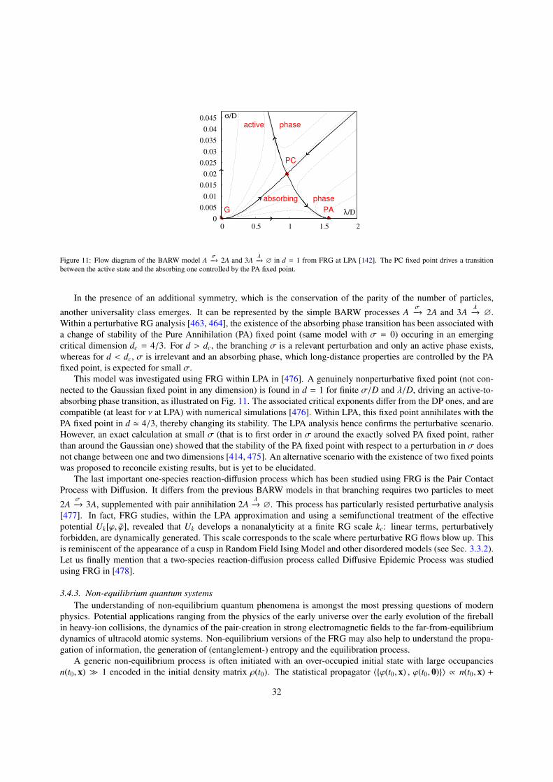
0
0.005
0.01
0.015
0.02
0.025
0.03
0.035
0.04
0.045
0 0.5 1 1.5 2
PC
PAG
σ/D
λ/D
active phase
absorbing phase
Figure 11: Flow diagram of the BARW model Aσ−→ 2A and 3A
λ−→ ∅ in d = 1 from FRG at LPA [142]. The PC fixed point drives a transition
between the active state and the absorbing one controlled by the PA fixed point.
In the presence of an additional symmetry, which is the conservation of the parity of the number of particles,
another universality class emerges. It can be represented by the simple BARW processes Aσ−→ 2A and 3A
λ−→ ∅.
Within a perturbative RG analysis [463, 464], the existence of the absorbing phase transition has been associated witha change of stability of the Pure Annihilation (PA) fixed point (same model with σ = 0) occuring in an emergingcritical dimension dc = 4/3. For d > dc, the branching σ is a relevant perturbation and only an active phase exists,whereas for d < dc, σ is irrelevant and an absorbing phase, which long-distance properties are controlled by the PAfixed point, is expected for small σ.
This model was investigated using FRG within LPA in [476]. A genuinely nonperturbative fixed point (not con-nected to the Gaussian fixed point in any dimension) is found in d = 1 for finite σ/D and λ/D, driving an active-to-absorbing phase transition, as illustrated on Fig. 11. The associated critical exponents differ from the DP ones, and arecompatible (at least for ν at LPA) with numerical simulations [476]. Within LPA, this fixed point annihilates with thePA fixed point in d ' 4/3, thereby changing its stability. The LPA analysis hence confirms the perturbative scenario.However, an exact calculation at small σ (that is to first order in σ around the exactly solved PA fixed point, ratherthan around the Gaussian one) showed that the stability of the PA fixed point with respect to a perturbation in σ doesnot change between one and two dimensions [414, 475]. An alternative scenario with the existence of two fixed pointswas proposed to reconcile existing results, but is yet to be elucidated.
The last important one-species reaction-diffusion process which has been studied using FRG is the Pair ContactProcess with Diffusion. It differs from the previous BARW models in that branching requires two particles to meet
2Aσ−→ 3A, supplemented with pair annihilation 2A
λ−→ ∅. This process has particularly resisted perturbative analysis
[477]. In fact, FRG studies, within the LPA approximation and using a semifunctional treatment of the effectivepotential Uk[ϕ, ϕ], revealed that Uk develops a nonanalyticity at a finite RG scale kc: linear terms, perturbativelyforbidden, are dynamically generated. This scale corresponds to the scale where perturbative RG flows blow up. Thisis reminiscent of the appearance of a cusp in Random Field Ising Model and other disordered models (see Sec. 3.3.2).Let us finally mention that a two-species reaction-diffusion process called Diffusive Epidemic Process was studiedusing FRG in [478].
3.4.3. Non-equilibrium quantum systemsThe understanding of non-equilibrium quantum phenomena is amongst the most pressing questions of modern
physics. Potential applications ranging from the physics of the early universe over the early evolution of the fireballin heavy-ion collisions, the dynamics of the pair-creation in strong electromagnetic fields to the far-from-equilibriumdynamics of ultracold atomic systems. Non-equilibrium versions of the FRG may also help to understand the propa-gation of information, the generation of (entanglement-) entropy and the equilibration process.
A generic non-equilibrium process is often initiated with an over-occupied initial state with large occupanciesn(t0, x) � 1 encoded in the initial density matrix ρ(t0). The statistical propagator 〈{ϕ(t0, x) , ϕ(t0, 0)}〉 ∝ n(t0, x) +
32

1/2 is first dominated by the large occupancies and the respective physics is well described by classical-statisticalapproximations to the full system. In O(N)-theories this classical-statistical regime is captured well by next-to-leadingorder computations in 1/N-expansions (s-channel resummations) of 2PI-hierarchies, for reviews see e.g. [479, 480].
For occupancies n(t0, x) ≈ 1 the quantum 1/2 in n(t0, x) + 1/2 gets sizable. The system enters a regime withnon-equilibrium quantum dynamics which requires a non-equilibrium quantum field theoretical description. This canbe done within the Schwinger-Keldysh formalism on a closed time path C with an initial density matrix ρ(t0) at theinitial time t0. Then, the real-time FRG follows straightforwardly with the standard cutoff term quadratic in the fields.In the scalar case, the generating functional for non-equilibrium correlation functions is given by
Zk[J; ρ] = Tr ρ(t0) exp{
iˆC
ϕ(x)J(x) +i2
ˆϕ(x)Rk(x, y)ϕ(y)
}, (57)
where x, y live on the Keldysh contour C. For an introduction to the formulation with a standard spatial-momentumcutoff see [406]. A manifestly causal cutoff is obtained if closing the Keldysh contour at a finite time t = τ. Then thecutoff parameter is simply the maximal time k = τ. The respective flow equation does not integrate-out momentum-shells but simply propagates the system in time, see [403, 404, 481, 482]. The regularisation can also be introducedvia deformations of the occupancies n(t, x)→ nk(t, x), see e.g. [401, 402] for applications in low-dimensional systems.
The Schwinger-Keldysh formulation of the FRG has been applied to the time evolution and turbulent cascades atnon-thermal fixed points in O(N)-models, [403, 482, 483], to the classification of dynamical critical phenomena inmodels with and without driving force, [407, 416, 484, 485], and to the cosmological power spectrum, [404, 486–490],see also [491]. For further applications in low-dimensional systems see also Sec. 4.2.4.
4. Quantum many-particle systems
Quantum many-particle theory was developed to describe interacting particles in condensed matter, and is nowrelevant for ultracold atomic gases, too. According to the two types of quantum statistics (leaving anyons aside), thisbroad field is naturally divided in the theory of interacting bosons and interacting fermions. Applications of the FRGto quantum many-particle problems have already been summarized in two extensive review articles published in 2012,one in relation to cold atoms [492], the other with a focus on interacting fermions in condensed matter [493].
We note in passing that the FRG can also be applied to few-body systems. A beautiful example is the Efimoveffect related to the formation of bound states of three or four interacting bosons or fermions, which is associated witha limit cycle in the renormalization group flow [494].
4.1. Bosons
The first realization of an interacting quantum Bose system was liquid 4He. Nowadays, ultracold bosonic atomsprovide a vast additional playground for exploring interaction effects in Bose systems. Moreover, interacting Bosesystems also emerge in effective low-energy theories. In the following we review a selection of systems where theFRG has made a major impact.
4.1.1. Superfluidity in a dilute Bose gasThe Euclidean action of a dilute Bose gas reads
S =
ˆ β
0dτˆ
ddr{ψ∗
(∂τ − µ −
∇2
2m
)ψ +
g2
(ψ∗ψ)2}, (58)
where the complex field ψ satisfies periodic boundary conditions, ψ(r, τ) = ψ(r, τ+β), and µ is the chemical potential.Most physical low-energy properties depend only on the boson mass m and the s-wave scattering length a ≡ a(g,Λ),which is a function of the repulsive interaction g and the upper momentum cutoff Λ in the model defined by (58). Forany finite density (µ > 0), the ground state is superfluid and characterized by spontaneously broken U(1) symmetry:〈ψ(r, τ)〉 , 0.
In three dimensions (and at zero temperatures in two dimensions) most physical properties of the superfluid phase,including the equation of state and the sound mode with linear dispersion, can be understood from the Bogoliubov
33

Figure 12: (left) Phase diagram of the 3D Bose-Hubbard model showing the first Mott lobe (with a density n = 1) and the surrounding superfluidphase. The solid (red) line shows the FRG result and the (green) dashed line the mean-field one. The QMC and DMFT data are obtained fromRefs. [531] and [532], respectively . (right) Phase diagram of the 2D Bose-Hubbard model. The QMC data are obtained from Ref. [533]. Reprintedfrom Ref. [232].
theory [495], based on a Gaussian-fluctuation approximation about the mean-field solution. Nevertheless, perturba-tion theory beyond the Bogoliubov approximation is plagued with infrared divergences [496–499]. Although thesedivergences cancel out in gauge-invariant quantities (pressure, sound velocity, etc.), they have a definite physicalorigin since they reflect the divergence of the longitudinal susceptibility, a phenomenon which also occurs in the low-temperature phase of the O(N ≥ 2) model (Sec. 2.3.2) but is not accounted for in the Bogoliubov theory. Popov hasproposed an approach to superfluidity, based on an amplitude-phase representation of the boson field, which is freeof infrared divergences and yields the correct low-energy behavior of the correlation functions but is restricted to the(low-momentum) hydrodynamic regime [500, 501].
Field-theoretical diagrammatic methods [502–504] or perturbative RG constrained by Ward identities [505, 506]can be used to handle the infrared divergences of perturbative theory. The FRG provides us with a simple alterna-tive method, free of any divergences, which encompasses both the Bogoliubov theory (valid, stricto sensu, only atmomenta larger than a “Ginzburg” scale) and Popov’s hydrodynamic approach [507]. It has been used to understandvarious properties of three- and two-dimensional superfluid Bose systems, from the equation of state to the excitationspectrum and the damping of quasi-particles [173, 244, 245, 340, 508–517].
Another important issue regarding dilute Bose gases is the determination of the superfluid transition temperature.In the absence of interactions (a = 0), the bosons undergo a Bose-Einstein condensation at the temperature T 0
c =
(2π/m)[n/ζ(3/2)]2/3 in three dimensions where n is the mean density. For weak interactions, the shift ∆Tc/T 0c =
(Tc − T 0c )/T 0
c in the transition temperature is a universal function of na3. The dependence of ∆Tc/T 0c on a has
remained a controversial issue for a long time and even the sign of the effect has been debated [518–520]. It is nowunderstood that ∆Tc/T 0
c = c(an1/3) increases linearly with a [521–525] and the proportionality coefficient c has beenestimated from various approaches. The difficulty in getting a precise estimate of c comes from the fact that it requiresthe knowledge of the one-particle propagator at Tc in a large momentum range including the crossover region betweenthe critical and noncritical regimes. The determination of c is therefore a nonperturbative problem which can be dealtwith the FRG. Since the full knowledge of the momentum dependence of the propagator is required, the DE is notsufficient. The BMW approximation (Sec. 2.4) gives c ' 1.37 [121, 122, 526] in reasonable agreement with latticeresults (c = 1.32(2) [527] and c = 1.29(5) [528]) and seven-loop resummed calculations (c = 1.27(10) [529]). AnotherFRG calculation, based on a vertex expansion, gives c = 1.23 [210, 530]. In the case of a model with N-componentreal fields (Eq. (58) corresponds to N = 2), the value of c obtained from FRG is remarkably accurate for N ≥ 3, beingwithin the error bars of lattice simulations and seven-loop calculations [122].
4.1.2. Superfluid to Mott-insulator transitionThe simplest model describing bosons moving in a d-dimensional hypercubic lattice is the one-band Bose-
Hubbard model defined by the action [534]
S =
ˆ β
0dτ
{∑r
[ψ∗r(∂τ − µ)ψr +
U2
nr(nr − 1)]− t
∑〈r,r′〉
(ψ∗rψr′ + h.c.
)}, (59)
34

-8 -4 0 4 8
-0.4
-0.3
-0.2
-0.1
0
x
ϑ(x,0)
-12 -8 -4 0 4 8 12
-0.6
-0.4
-0.2
0
x
-12 -8 -4 0 4 8 12
-1
-0.8
-0.6
-0.4
-0.2
0
-12 -8 -4 0 4 8 12
-0.8
-0.4
0
x
Figure 13: Scaling function ϑ(x, 0) determining the singular part of the internal energy density, εsing(δ,T ) = ϑ(x, 0)(kBT )3/(~c)2 (c is the velocity ofthe critical fluctuations), in the two-dimensional quantum O(N) model near its quantum critical point (full lines); x ∝ δ/T 1/ν where δ measures thedistance to the quantum critical point and ν is the correlation-length critical exponent of the T = 0 phase transition. The symbols show the resultsobtained from Monte Carlo simulations of three-dimensional classical spin models in a finite geometry where ϑ(x, 0) determines the universalCasimir force. The horizontal dashed line shows the (exact) limit −2(N−1)ζ(3)/2π for x→ −∞. (left panel) Ising (N=1) universality class. MonteCarlo simulations are from Ref. [536] (blue diamonds), Ref. [537] (green squares) and Ref. [538] (red circles). (middle panel) XY universalityclass (N=2). The Monte Carlo data are from Ref. [536]. (right panel) Heisenberg universality class (N=3). The Monte Carlo data [539] have beenrescaled so as to satisfy the correct asymptotic value for x→−∞, the bare data are shown in the inset. Reprinted from Ref. [172].
where nr = ψ∗rψr, U is the on-site repulsion, t the intersite hopping amplitude, and 〈r, r′〉 denotes nearest-neighborsites. When the average number n of bosons per site is integer and U � t, the ground state is a Mott insulator with nbosons localized at each lattice site, a vanishing compressibility κ = ∂n/∂µ and a gap in the excitation spectrum. Atransition to a superfluid ground state can be induced by either decreasing the ratio U/t or varying n. In the first casethe transition is in the universality class of the (d+1)-dimensional XY (or O(2)) model with an upper critical dimensiond+
c = 3. In the second one, the transition is in the universality class of the dilute Bose gas and is mean-field-like abovetwo dimensions (d+
c = 2).The three- and two-dimensional Bose-Hubbard models have been studied within the FRG approach using the
lattice formulation (Sec. 2.5) where the initial condition corresponds to the limit of decoupled sites [231, 232]. TheFRG yields a phase diagram in very good agreement with the (numerically exact) quantum Monte Carlo simula-tions [531, 533] and with an accuracy similar to that obtained from dynamical-mean-field theory [532, 535]; seeFig. 12. It also allows one to compute nonuniversal quantities such as the velocity (or the effective mass when thetransition is induced by a density change) of the critical fluctuations. It reproduces the two universality classes of thesuperfluid–Mott-insulator transition and gives an accurate determination of the universal scaling functions associatedwith the equation of state near the quantum critical point [171, 233, 234].
4.1.3. Relativistic bosons and quantum O(N) modelThe simplest quantum generalization of the O(N) model discussed in Sec. 2, with space-time Lorentz invariance,
is defined by the Euclidean (imaginary-time) action
S [ϕ] =
ˆ β
0dτˆ
ddr{1
2(∇ϕ)2 +
12c2 (∂τϕ)2 +
r0
2ϕ2 +
u0
4!(ϕ2)
2}, (60)
where the N-component real field satisfies periodic boundary conditions: ϕ(r, τ) = ϕ(r, τ + β). r0 and u0 aretemperature-independent coupling constants and c is the (bare) velocity of the excitations. The quantum O(2) modeldescribes relativistic bosons and is relevant for the superfluid–Mott-insulator transition (Sec. 4.1.2); the N = 3 modelapplies to quantum antiferromagnets, the N = 4 to QCD, etc. At zero temperature the quantum model is equivalentto its (d + 1)-dimensional classical counterpart and therefore exhibits a quantum phase transition between a disor-dered phase and an ordered phase where the O(N) symmetry is spontaneously broken. At nonzero temperature theequivalent classical model has a finite size Lτ = β in the (d + 1)th dimension. The finite-temperature thermodynamichas been studied within the FRG approach [170, 540, 541]. In the vicinity of the quantum critical point, the scalingfunctions determining the universal equation of state [172] are in striking agreement with Monte Carlo simulations of(d +1)-dimensional classical N-component spin models in a finite geometry (these models are in the same universalityclass as the two-dimensional quantum O(N) model) [536–539]; see Fig. 13.
35

Momentum-frequency dependent correlation functions and spectral functions of the quantum O(N) model havealso been obtained from the FRG. In the context of QCD, where the O(4) model is frequently used as a chiral effectivemodel, spectral functions of sigma mesons and pions have been computed [253, 254, 257, 259]. In statistical physics,the FRG approach has lead to the confirmation of the existence of a bound state in the ordered phase of the two-dimensional quantum O(1) model [165], with a mass within 1% of previous Monte Carlo simulations and numericaldiagonalization values [542–544]. In the ordered phase of the two-dimensional O(2) and O(3) models, the “Higgs”amplitude mode, whose existence and visibility in the vicinity of the quantum critical point have been overlooked for along time [545], is well described by FRG [221, 546], in quantitative agreement with Monte Carlo simulations [547].The estimate of the “Higgs” mass in the quantum O(3) model from the BMW approach has been confirmed bysubsequent exact diagonalizations [548, 549] and quantum Monte Carlo simulations of quantum spin models [550].At zero-temperatures, the frequency-dependent conductivity and its universal features have also been studied [120,247, 551].
4.2. Fermions
Interacting fermion systems display a particularly rich variety of phases and phenomena. The most importantrepresentatives are electrons in solids, liquid 3He, and ultracold fermionic atoms. In this section we focus on non-relativistic systems with spin- 1
2 fermions.For fermions moving in a continuum, the bare Euclidean action has the form [552]
S [ψ, ψ∗] =
ˆ β
0dτˆ
ddr ψ∗(r, τ)(∂τ − µ −
12m∇2
r
)ψ(r, τ) + V[ψ, ψ∗] , (61)
where ψ = (ψ↑, ψ↓) and ψ∗ = (ψ∗↑, ψ∗↓) are anticommuting spinor fields with antiperiodic boundary conditions in τ, and
V[ψ, ψ∗] is an arbitrary interaction term. For two-particle interactions, V[ψ, ψ∗] is quartic in the fields. Note that ψ andψ∗ are independent variables. For lattice fermions, the space variable r is replaced by a discrete lattice site variable j,and the gradient term by hopping amplitudes between sites j and j′.
The Fermi-Dirac statistics of the particles and the existence of a Fermi surface at nonzero density leads to a numberof difficulties that are not present in the bosonic case discussed in the previous section. First, the fermionic effectiveaction Γk[ψ, ψ∗] defined below is a functional of Grassmann variables. As pointed out in Sec. 2.6, one must thereforetruncate Γk[ψ∗, ψ] in an expansion about ψ = ψ∗ = 0, which amounts to retaining only a finite number of verticesand performing a loop expansion of the flow equations. This makes the fermionic FRG fundamentally perturbative.Second, since the low-energy fermion states live near the Fermi surface, it is not possible to neglect the momentumdependence of the vertices Γ
(n)k or perform a derivative expansion, i.e., an expansion about momentum p = 0. Thus
the vertices are necessarily functionals of the momenta.27 Third, the Grassmannian field is not an order parameter;order parameters are defined by composite fields: 〈ψ∗ψ〉 for a charge- or spin-density wave, 〈ψψ〉 for a superconductor.A phase transition is signaled by a divergence of the associated susceptibility and the two-particle vertex Γ
(4)k . The
growth of Γ(4)k implies a breakdown of the (perturbative) RG and prevents, at least in a straightforward way, to continue
the flow into the ordered phase. Furthermore, the fluctuations of the bosonic fields ψ∗ψ and ψψ being not properlytaken care of, the flow becomes uncontrolled whenever strong collective fluctuations with a large correlation lengthset in. We shall discuss below how one can, at least partially, overcome these difficulties, e.g., by introducing bosonicfields to take into account collective fluctuations or starting the FRG flow from a nonperturbative initial condition.
The FRG for interacting fermion systems and various applications have already been reviewed in Ref. [493]. Thatreview also contains a short history of the renormalization group for fermion systems which shall not be repeatedhere. In the meantime, there have been substantial methodological developments, and the range of applications hasbroadened considerably. A concise review covering also rigorous mathematical work has been published recently bySalmhofer [553].
27In the fermionic case, the terminology functional RG originally stems from the momentum dependence of the vertices and not their fielddependence.
36

d
d
dk
dΓ
(4)
dkΓ
(6)
= Γ
S
(4)
+
ΓΓΓ(4)
=
(4)
+ +
Γ (6)
=
Γ(4)
(4)
Γ(4)
S
S
Γ (8)Γ
(4)
S G
kΣ
d
(6)
k
k
k
k
k k
k
k
k
k
k
k
k
k
k
Γk
k
k
Gk
Gk
Gk
Sk
Sk
Figure 14: Diagrammatic representation of the flow equations for the self-energy Σk , the two-particle vertex Γ(4)k , and the three-particle vertex Γ
(6)k
in the one-particle irreducible version of the functional RG. Lines with a dash correspond to the single scale propagator S k (shown as a line with across in Fig. 2), the other lines correspond to the full propagator Gk .
4.2.1. Fermion flow equationThe scale dependent effective action and its flow equation are obtained in close analogy to the classical O(N)
model described in Sec. II. The flow is defined by adding a scale dependent regulator term ∆S k = −(ψ∗,Rkψ) =
−´
dx´
dx′ψ∗(x′)Rk(x′, x)ψ(x) to the bare action, where x and x′ include space and time variables (or, alternatively,momentum and frequency variables), and k is the flow parameter.28 Here and in the following (., .) is a shorthandnotation for the summation (or integration) over all fermion field indices in an arbitrary basis. The regulator termmodifies the bare propagator G0 to G0,k = (G−1
0 + Rk)−1. The effective action is defined by the Legendre transform ofthe free energy in the presence of Grassmann source fields
Γk[ψ, ψ∗] = − lnZk[ηk, η∗k] + (η∗k, ψ) + (ψ∗, ηk) − ∆S k[ψ, ψ∗] , (62)
where ηk and η∗k are k-dependent functions of ψ and ψ∗, as determined by the equations ψ = ∂η∗ lnZk[η, η∗] andψ∗ = −∂η lnZk[η, η∗].
The fermionic version of Wetterich’s exact flow equation for the effective action reads [60, 493]
∂kΓk[ψ, ψ∗] = −12
Tr{∂kRk
(Γ
(2)k [ψ, ψ∗] + Rk
)−1}, (63)
where
Γ(2)k [ψ, ψ∗](x′, x) =
∂2Γk
∂ψ∗(x′)∂ψ(x)∂2Γk
∂ψ∗(x′)∂ψ∗(x)
∂2Γk∂ψ(x′)∂ψ(x)
∂2Γk∂ψ(x′)∂ψ∗(x)
, (64)
and Rk(x′, x) = diag[Rk(x′, x),−Rk(x, x′)]. Note that Γ(2)k is a functional of the fields and a function of the field
indices. The matrix structure of the two-point function generated by the conjugated variables ψ and ψ∗ gives rise toparticle-particle and particle-hole channels in fermion systems.
Expanding the functional flow equation (63) in powers of the fields, one obtains an exact hierarchy of flow equa-tions for the vertex functions [60, 493]. For fermions, there are only vertex functions of even order in the fields. InFig. 14 we show the Feynman diagrams describing the first three equations in the hierarchy. One of the internal linescorresponds to the single-scale propagator
S k = −Gk(∂kRk)Gk = ∂kGk
∣∣∣Σk const , (65)
28In the literature on interacting fermion systems the greek letter Λ is the most commonly used symbol for the flow parameter. However, for thesake of a consistent notation within this review, we denote the flow parameter by k.
37

������������������������������������������������������������������������������������������
������������������������������������������������������������������������������������������
−π
−π 0 π
0
py
px
π
Figure 15: Momentum space region around the Fermi surface excluded by a sharp momentum cutoff for fermions with a tight-binding dispersionon a two-dimensional square lattice (lattice constant a = 1).
where Gk = (G−10,k − Σk)−1 is the full scale-dependent propagator.
The non-interacting propagator in a translation and spin-rotation invariant system has the spin-independent andmomentum-diagonal form
G0(p, iωn) =[iωn − (εp − µ)
]−1, (66)
where εp is the energy of single-particle states with momentum p, and ωn = (2n + 1)πT with integer n is the fermionicMatsubara frequency. At T = 0 the propagator diverges for ωn = 0 and εp = µ, that is, for momenta on the Fermisurface. Hence, in fermion systems with dimensionality d > 1 the propagator exhibits an extended singularity, notjust a divergence at a point in momentum space.
There are various possibilities to regularize the Fermi surface singularity in the FRG flow. One is to choose amomentum dependent regulator that suppresses contributions with momenta close to the Fermi surface. An extremechoice is a sharp momentum cutoff, where contributions from momenta p with |εp − µ| < k are completely suppressed(see Fig. 15). This corresponds to a regularized bare propagator of the form G0,k = Θ(|εp − µ| − k)G0. Of course onemay also choose a smooth momentum cutoff. In any case, for fermion systems momentum cutoffs have two majordrawbacks. First, the Fermi surface can actually be deformed by interactions, so that the regulator cannot be fixeda priori, if these deformations are taken into account. Second, the limit of vanishing momentum transfer q → 0 ininteraction vertices does not commute with the limit k → 0 for momentum cutoffs [554]. Both of these problems canbe avoided by choosing a frequency cutoff [555], which is therefore the most popular choice nowadays. A frequencycutoff can also be used in systems without translation invariance [556]. Alternatively one may use the interaction[557] or temperature [558] as flow parameters. The interaction flow is computationally convenient, but it does notregularize the Fermi surface singularity.
4.2.2. Competing instabilitiesAt low temperatures, the normal metallic state of interacting fermion systems is usually unstable toward mag-
netism, superconductivity, or more exotic forms of order. For systems with weak or moderate interaction strengths,the FRG has turned out to be a valuable tool for the unbiased detection of instabilities, especially in cases whereseveral instabilities of distinct nature compete with each other.
Most instabilities are signalled by a divergence of the two-particle vertex Γ(4)k . For weak interactions, the flow of
Γ(4)k can be truncated at second order, that is, contributions from the self-energy and the three-particle vertex can be
neglected such that only the first Feynman diagram in the second line of Fig. 14 needs to be computed. Writing outthe various terms arising from the matrix structure of Γ
(2)k [ψ, ψ∗] in Eq. (64), one obtains three types of contributions
to the flow of Γ(4)k , known as particle-particle, direct particle-hole, and crossed particle-hole channel, respectively (see
Fig. 16).The two-particle vertex is a function of four momenta and four Matsubara frequencies. The latter are constrained
by energy conservation to three independent frequencies, and for translation invariant systems momentum conserva-tion also reduces the number of independent momenta to three. The flow needs to be computed numerically, and asuitable parametrization of the two-particle vertex is a major issue. In weak coupling power counting, the frequency
38

2
1 1’
2’
= pp
1
2 2
2’ 2’1
1’ 1’
1
2 2
1’1’
2’ 2’
1
ph ph’
Γddk
(4)
k
Figure 16: Contributions to the flow of the two-particle vertex with particle-particle (pp) and particle-hole channels (ph and ph’) written explicitly,without the contribution from Γ
(6)k .
dependence and the momentum dependence perpendicular to the Fermi surface appear to be irrelevant [559]. Hence,in most concrete evaluations of the vertex flow the frequency dependence of the vertex was neglected, and the mo-mentum dependence was discretized by a partition of momentum space in patches, paying particular attention to anaccurate resolution of the dependences along the Fermi surface. With N patches one thus obtains O(N3) “runningcouplings”, where discrete symmetries can be exploited to reduce the precise number to a certain fraction of N3.
The nature of the instabilities can be read off from the momentum and spin dependence of the diverging two-particle vertex. For example, pairing instabilities are signalled by a divergence in the Cooper channel, that is, for avanishing total ingoing and outgoing momentum. To identify the instabilities it can also be helpful to analyze thecorresponding susceptibilities, for which flow equations can be derived by adding external symmetry breaking fieldsto the bare action [493].
Two-dimensional Hubbard model: The FRG stability analysis was originally developed for the two-dimensionalone-band Hubbard model, describing tight-binding fermions with a local interaction on a square lattice. The Hamil-tonian is given by
H =∑j,j′
∑σ
tjj′c†
j′σcjσ + U∑
j
nj↑nj↓ (67)
in standard second quantization notation, where tjj′ are hopping amplitudes between sites j and j′ and U is a localinteraction. The two-dimensional Hubbard model was proposed by Anderson [560] as an effective model for electronsmoving in the copper-oxygen planes of cuprate high temperature superconductors. At half-filling, that is, for anaverage fermion density n = 1, the ground state of the 2D Hubbard model is an antiferromagnetic insulator forsufficiently large U. The critical U depends on the structure of the hopping matrix. For pure nearest neighbor hoppingany positive U leads to an antiferromagnetic ground state. While the magnetic instability in the Hubbard model isrevealed already by conventional mean-field theory, pairing is fluctuation-driven and hence more difficult to capture.Simple qualitative arguments suggesting d-wave pairing driven by magnetic fluctuations were corroborated by thefluctuation exchange approximation, that is, a resummation of a certain class of Feynman diagrams in perturbationtheory [561]. However, only the unbiased stability analysis made possible by the FRG provided conclusive evidencefor the existence of d-wave superconductivity with a sizable energy gap at moderate interaction strength, since the FRGtreats all fluctuation channels on equal footing. The first FRG results for the Hubbard model were actually obtainedfrom three distinct FRG versions, namely Polchinski’s flow equation [562, 563], a Wick ordered flow equation [564,565], and the Wetterich equation [566].
In Fig. 17 (left panel) we show the ground state phase diagram of the 2D Hubbard model for a nearest neighborhopping amplitude t and a next-to-nearest neighbor hopping amplitude t′ = −0.01t in the weak coupling regime, asobtained from the FRG flow with a momentum cutoff [565]. Each symbol in the plot corresponds to a choice of µ andU for which the dominant instability was identified from divergences of the two-particle vertex and susceptibilitiesat a critical cutoff kc. In Fig. 17 (right panel) we show the pseudocritical temperature, at which the two-particle
39
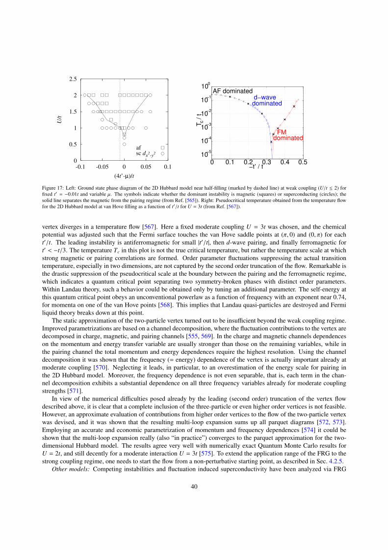
0
0.5
1
1.5
2
2.5
-0.1 -0.05 0 0.05 0.1
U/t
(4t’-µ)/t
af sc dx
2-y
2
0 0.1 0.2 0.3 0.4 0.5
10−5
10−4
10−3
10−2
10−1
100
AF dominated
d−wave dominated
FM dominated
−t’ / t
Tc /
t
Figure 17: Left: Ground state phase diagram of the 2D Hubbard model near half-filling (marked by dashed line) at weak coupling (U/t ≤ 2) forfixed t′ = −0.01t and variable µ. The symbols indicate whether the dominant instability is magnetic (squares) or superconducting (circles); thesolid line separates the magnetic from the pairing regime (from Ref. [565]). Right: Pseudocritical temperature obtained from the temperature flowfor the 2D Hubbard model at van Hove filling as a function of t′/t for U = 3t (from Ref. [567]).
vertex diverges in a temperature flow [567]. Here a fixed moderate coupling U = 3t was chosen, and the chemicalpotential was adjusted such that the Fermi surface touches the van Hove saddle points at (π, 0) and (0, π) for eacht′/t. The leading instability is antiferromagnetic for small |t′/t|, then d-wave pairing, and finally ferromagnetic fort′ < −t/3. The temperature Tc in this plot is not the true critical temperature, but rather the temperature scale at whichstrong magnetic or pairing correlations are formed. Order parameter fluctuations suppressing the actual transitiontemperature, especially in two dimensions, are not captured by the second order truncation of the flow. Remarkable isthe drastic suppression of the pseudocritical scale at the boundary between the pairing and the ferromagnetic regime,which indicates a quantum critical point separating two symmetry-broken phases with distinct order parameters.Within Landau theory, such a behavior could be obtained only by tuning an additional parameter. The self-energy atthis quantum critical point obeys an unconventional powerlaw as a function of frequency with an exponent near 0.74,for momenta on one of the van Hove points [568]. This implies that Landau quasi-particles are destroyed and Fermiliquid theory breaks down at this point.
The static approximation of the two-particle vertex turned out to be insufficient beyond the weak coupling regime.Improved parametrizations are based on a channel decomposition, where the fluctuation contributions to the vertex aredecomposed in charge, magnetic, and pairing channels [555, 569]. In the charge and magnetic channels dependenceson the momentum and energy transfer variable are usually stronger than those on the remaining variables, while inthe pairing channel the total momentum and energy dependences require the highest resolution. Using the channeldecomposition it was shown that the frequency (= energy) dependence of the vertex is actually important already atmoderate coupling [570]. Neglecting it leads, in particular, to an overestimation of the energy scale for pairing inthe 2D Hubbard model. Moreover, the frequency dependence is not even separable, that is, each term in the chan-nel decomposition exhibits a substantial dependence on all three frequency variables already for moderate couplingstrengths [571].
In view of the numerical difficulties posed already by the leading (second order) truncation of the vertex flowdescribed above, it is clear that a complete inclusion of the three-particle or even higher order vertices is not feasible.However, an approximate evaluation of contributions from higher order vertices to the flow of the two-particle vertexwas devised, and it was shown that the resulting multi-loop expansion sums up all parquet diagrams [572, 573].Employing an accurate and economic parametrization of momentum and frequency dependences [574] it could beshown that the multi-loop expansion really (also “in practice”) converges to the parquet approximation for the two-dimensional Hubbard model. The results agree very well with numerically exact Quantum Monte Carlo results forU = 2t, and still decently for a moderate interaction U = 3t [575]. To extend the application range of the FRG to thestrong coupling regime, one needs to start the flow from a non-perturbative starting point, as described in Sec. 4.2.5.
Other models: Competing instabilities and fluctuation induced superconductivity have been analyzed via FRG
40

Σ
= =
G
d
dk
d
dk
G.
k
k
k
k
S
Γk
Γ Γk k
Γk
(4) (4) (4) (4)
Figure 18: Katanin truncation for the coupled flow of self-energy and two-particle vertex.
flows of the two-particle vertex for numerous other models. For multi-orbital systems, such as pnictide superconduc-tors, the unitary transformation from orbital to band operators leads to momentum dependences already in the barevertex, even for local (Hubbard-type) interactions [576, 577]. FRG flows have provided valuable information on in-stabilities of various compounds, especially of those where electron-electron interactions are weak or moderate. It isbeyond the scope of this review to list all these applications here. Some of the earlier applications have been describedin Ref. [493]. A more extensive review of work on multi-orbital systems performed before 2013, in particular onpnictides and compounds with hexagonal lattices (triangular, honeycomb, and Kagome), has been published by Plattet al. [578]. Since then the range of applications has significantly broadened, often following experimental discover-ies, including systems with spin-orbit coupling [579], new Dirac nodal-line materials [580] and, most recently, moireheterostructures [581], to name just a few.
4.2.3. Spontaneous symmetry breakingIn most interacting fermion systems a symmetry of the Hamiltonian is spontaneously broken at sufficiently low
temperatures, or at least in the ground state. In the FRG flow, common types of symmetry breaking such as magneticorder or superconductivity are associated with a divergence of the two-particle vertex at a finite scale kc > 0. Onemay encounter a divergence even in cases where ultimately only quasi-long range order or two-particle bound statesare formed. To continue the flow beyond this critical scale, an order parameter needs to be implemented. There aretwo distinct ways of doing this.
Fermionic flows: In one approach the FRG flow is computed in the presence of a small (ideally infinitesimal)symmetry breaking field added to the bare action, which develops into a finite order parameter below the scale kc [582].The external field regularizes the divergence of the vertex at kc. This field can be endowed with a scale-dependence,so that it can be removed completely at the end of the flow [583]. One then needs to apply a manageable truncation ofthe exact flow equations which does not break down at the critical scale where the two-particle vertex becomes largeeven for a weak bare interaction. A minimal requirement is that a truncation should at least provide a decent solutionfor mean-field models, such as the reduced BCS model. The simplest approximation satisfying this requirement is theKatanin truncation [584] shown in Fig. 18. Here the single-scale propagator S k in the leading contribution to the flowof the two-particle vertex (cf. Fig. 14) has been replaced by ∂kGk. This takes self-energy corrections generated by thethree-particle vertex into account, while other contributions from the three-particle vertex are neglected. Spontaneoussymmetry breaking leads to anomalous contributions to both the self-energy and the two-particle vertex. The flowobtained from Katanin’s truncation solves the reduced BCS model and similar mean-field models for other types oforder exactly [582, 585]. In spite of the diverging two-particle interaction the neglected contributions do not contributebecause of a zero-measure momentum integration region.
The Katanin truncation has been used as an approximation to compute ground state order parameters for the two-dimensional Hubbard model with attractive and repulsive interactions. For the attractive Hubbard model, the s-wavepairing gap obtained from the FRG flow [583, 586] is substantially suppressed compared to mean-field theory even atweak coupling, in agreement with results from other methods. For the repulsive Hubbard model, the d-wave pairinggap was computed for weak and moderate interactions, and it was shown that a sizable next-to-nearest neighborhopping amplitude is beneficial for d-wave superconductivity [587]. The Ward identity protecting gapless Goldstonemodes in phases with a broken continuous symmetry is not automatically satisfied by the Katanin truncation. However,one may enforce it by a suitable projection procedure [583].
Flows with order-parameter fields: Spontaneous symmetry breaking in interacting fermion systems can also betreated by introducing collective bosonic order parameter fields via a Hubbard-Stratonovich decoupling of the two-fermion interaction [588], and applying the FRG to the resulting coupled boson-fermion action. This route to symme-
41

try breaking was first used to treat the formation of an antiferromagnetic state in the repulsive 2D Hubbard model athalf-filling [589]. The correct low-temperature behavior (usually described by a nonlinear sigma model) was recov-ered from from a simple truncation of the exact flow equation. Spontaneous symmetry breaking sets in at a criticalscale kc, where the boson mass vanishes, but at finite temperatures the symmetry is gradually restored by bosonicfluctuations at lower scales, in agreement with the Mermin-Wagner theorem.
Subsequently, the coupled flow of fermions and bosonic order parameter fluctuations was applied to the superfluidphase of fermion systems with attractive interactions, using U(1)-symmetric truncations of the effective fermion-bosonaction. A simple truncation, where the bosonic part of the effective action has the form of a Bose gas with a local φ4
interaction, yields already sensible results for the pairing gap and the transition temperature in three dimensions in theentire range from BCS superfluidity at weak coupling to Bose-Einstein condensation of tightly bound pairs at strongcoupling [590–593]. To include effects from particle-hole fluctuations, which tend to reduce the pairing gap, one hasto take effective two-fermion interactions into account. Decoupling these at each step in the flow by a scale-dependent“dynamical bosonisation” [594, 595], one obtains a substantial quantitative improvement [596]. Instead of using aU(1)-symmetric ansatz for the effective action, it is also possible to start from the hierarchy of flow equations for thevertex functions and implement the U(1) symmetry via Ward identities [597].
To distinguish the Goldstone mode from longitudinal order parameter fluctuations in a U(1)-symmetric ansatz, oneneeds to include quartic gradient terms in the bosonic part of the effective action [112]. A relatively simple truncationof the complete effective action (for fermions and bosons) yields the correct low-energy behavior of the superfluidground state in dimensions d ≥ 2 [598].
The interplay of antiferromagnetism and superconductivity in the two-dimensional repulsive Hubbard model wasalso analyzed by FRG flows with order-parameter fields. It was clarified how d-wave pairing mediated by antiferro-magnetic fluctuations emerges from the coupled fermion-boson flow [599], and a phase diagram with magnetic andsuperconducting order was computed at weak coupling [600, 601].
Renormalized mean-field theory: In case of competing instabilities and possible coexistence of two or more orderparameters, both routes to symmetry breaking described above become quite involved. For a computation of orderparameters in the ground state one may neglect low-energy fluctuations and combine flow equations at high scales witha mean-field approximation at low scales [602, 603]. In this approach the flow of the two-particle vertex Γ
(4)k is stopped
at a scale kmf slightly above the critical scale kc, that is, before entering the symmetry-broken regime. The remaininglow-energy degrees of freedom are treated in mean-field approximation, with a reduced effective interaction extractedfrom Γ
(4)kmf
. An application of this renormalized mean-field theory revealed broad doping regions with coexistence ofd-wave superconductivity and Neel or incommensurate antiferromagnetic order in the ground state of the 2D Hubbardmodel [602–604].
FRG in the two-particle irreducible (2PI) formalism: Although the 2PI formalism in the framework of the FRGhas been considered in various contexts [67, 605–607], few works have focused on interacting fermions. In the 2PIapproach [608–613], the scale-dependent effective action Γk[G] is a functional of the one-particle propagator and theWetterich equation becomes a flow equation for the scale-dependent Luttinger-Ward functional Φk[G] [309, 614–616]. The “classical” variable is thus bosonic in nature and is itself an order parameter. There are no conceptualdifficulties to describe phases with spontaneously broken symmetries and one can even start the RG flow in a broken-symmetry phase (with the Hartree-Fock-RPA theory as initial condition). The 2PI formalism has been proposed as apossible approach to the Hubbard model [615], in particular in combination with dynamical mean-field theory [617](see Sec. 4.2.5). It has also been applied to quantum impurity models [618]. Finally, the 2PI FRG has been used inconnection with density functional theory to study many-body systems in condensed or nuclear matter [619–623].
4.2.4. Quantum transportElectronic transport through nanostructured devices such as quantum wires and quantum dots is an important
area in modern condensed matter physics. The typical setup is a mesoscopic region coupled to two or more leads.While the electrons in the leads move more or less independently, interesting correlation effects due to the restrictedgeometry can occur in the mesoscopic region [624].
In general, the calculation of transport properties in interacting systems requires the calculation of two-particlequantities such as current-current correlation functions [625]. Under certain assumptions, the electronic transportthrough a mesoscopic region can be viewed as a scattering problem, and the electric conductance can be written in the
42

Landauer-Buttiker form [626, 627]
C = −e2
2π
∑ζ
ˆdε Tζ(ε) f ′(ε) , (68)
where ζ labels the scattering channels, Tζ(ε) is the transmission probability for each channel, and f (ε) is the Fermifunction. Note that we use natural units where ~ = 1 such that the conductance quantum is e2/(2π). For a frequency-independent self-energy, Eq. (68) is actually exact, and the transmission probability can be expressed by the one-particle propagator at the contacts connecting the interacting region to the leads [628].
An important quantum transport problem involving correlated electrons is posed by electrons moving through aone-dimensional metallic wire with one or a few impurities [629, 630]. Interacting electrons in one-dimensional met-als form a Luttinger liquid [631], which, unlike Fermi liquids, has no resemblance to a Fermi gas. While perturbationtheory diverges at any interaction strength for these systems, a strikingly simple truncation of the FRG flow equationscaptures the most important effects related to non-magnetic impurities in one-dimensional metals [556, 632]. Indeed,already the first equation in the flow equation hierarchy (see Fig. 14), with the bare instead of the effective two-particlevertex, yields several power-laws describing the low-energy behavior, where the exponents are correct to leading orderin the interaction strength. Since the self-energy is frequency independent in this first order truncation, the conduc-tance can be computed without further approximations from the one-particle propagator [633]. The conductancethrough a wire with a single impurity vanishes with a power-law as a function of temperature as expected [629]. Incase of two impurities a rich behavior involving resonant tunneling and crossovers between distinct power-laws couldbe obtained [633, 634].
The same FRG approach turned out to be equally fruitful in a computation of persistent currents in a mesoscopicLuttinger liquid ring [635, 636], in a study of quantum transport through a Y-junction of three Luttinger liquid wires[637], and to describe transport through a correlated quantum dot setup dominated by charge fluctuations (absence ofthe Kondo effect) [638].
The FRG was also extended to steady-state nonequilibrium transport through quantum wires and quantum dotsin the presence of a finite voltage [402, 638, 639]. This extension makes use of real-time or real-frequency Greenfunctions on the Keldysh contour [640]. Compared to the equilibrium imaginary frequency FRG, in the steady statethe only technical complication is an additional Keldysh index ±. An important issue is to define a flow that does notviolate causality and Kubo-Martin-Schwinger (KMS) relations after truncation of the flow equation hierarchy [641].Suitable choices are a judiciously designed imaginary frequency cutoff [402, 641] or scale dependent local auxiliaryterms, which are removed at the end of the flow [250, 641]. The non-equilibrium FRG was applied to simple modelsof quantum dots [638] and quantum wires [402]. It is even possible to compute time-dependent non-equilibriumtransport of setups with correlated mesoscopic regions using Keldysh-FRG. This approach was used to study thequench dynamics of quantum dots [642] and quantum wires [643], as well as the dynamics of periodically drivensystems [644]. The FRG on the Keldysh contour can also be used to compute real frequency quantities in equilibrium,avoiding thus the numerically unstable analytic continuation from imaginary to real frequencies [250, 260].
4.2.5. Leap to strong couplingA truncation of the FRG hierarchy of flow equations at some finite order can be justified only for weak interactions
[645], with the exception of mean-field models where phase space restrictions suppress higher order contributions[582]. Although bare interactions are usually two-particle interactions, effective m-particle interactions with m > 2are generated by the flow and affect the effective two-particle interaction and the self-energy, see Fig. 14. For strongbare interactions, these contributions become important already at high energy scales far above the critical scalesfor instabilities. One of the most important strong coupling phenomena in correlated lattice electron systems likethe Hubbard model is the Mott metal-insulator transition. Cuprate high-temperature superconductors are doped Mottinsulators [560]. Truncated FRG flow equations starting from the bare action do not capture the Mott transition.
For interacting fermion systems there are no non-perturbative approximations such as the derivative expansion ofthe exact flow equation for bosons. However, one may choose a suitable non-perturbative approximation as a startingpoint for the flow. The Mott transition is essentially a consequence of strong local correlations. As such, it is welldescribed by the dynamical mean-field theory (DMFT), which treats local correlations non-perturbatively [646–648].The DMFT and the FRG can be consistently merged in the socalled DMF2RG [236, 237]. In this approach the FRGflow does not start from the bare action of the system, but rather from the DMFT solution. Strong local correlations
43

and the Mott physics are thus captured via the DMFT starting point, while the nonlocal correlations are generated bythe FRG flow. While an obvious small expansion parameter is still lacking, the weaker nonlocal correlations may becaptured by a manageable truncation of the exact FRG hierarchy. The flow can be defined such that it is generatedexclusively by non-local correlations [649].
Concrete DMF2RG calculations have so far been performed with a truncation of the flow equations at the two-particle level [237, 649], involving thus the two-particle vertex and the self-energy. For strong interactions, the two-particle vertex exhibits strong frequency dependencies which cannot be reduced to one frequency per interaction chan-nel. Nevertheless, numerical solutions of the DMF2RG flow equations have been obtained for the two-dimensionalHubbard model in the strong coupling regime, and evidence for d-wave pairing at the expected (for cuprates) temper-ature scale has been found [649].
Recently, a combination of the extended DMFT for non-local interactions with the 2PI version of the FRG hasbeen proposed [617]. Encouraging first benchmarks were obtained for the conventional and the extended Hubbardmodel at half-filling.
4.2.6. OmissionsThe range of applications of the FRG has become too broad to be covered in a single review. Here we briefly
mention two important devopments related to fermion systems which we could not review in detail.Spin systems: Using an auxiliary fermion representation of spin degrees of freedom, the FRG can also be applied
to quantum spin systems [650, 651]. The pseudofermions carry no kinetic energy, and the interactions depend onlyon one space or momentum variable. Using the Katanin truncation [584] of the flow equations and keeping thefull frequency dependence of the self-energy and interaction vertex leads to an approximation scheme that worksremarkably well for a variety of spin systems. This success of a perturbative truncatation for a strongly coupled systemcan be partially understood since leading orders in 1/N and 1/S expansions are captured by the approximation. Theaccuracy can be systematically improved by using decoupled clusters instead of single pseudo-fermions as startingpoint for an expansion [235]. Alternative ways of treating quantum spin systems with the FRG have been developedby mapping spins on hard core bosons [546] or working directly with spin operators [230].
Quantum criticality: Numerous quantum many-body systems undergo a continuous transition between groundstates with distinct symmetry or topology upon tuning a non-thermal control parameter. In the vicinity of the quantumcritical point separating the two phases, quantum fluctuations are particularly important and lead to unconventionalproperties not only in the ground states, but also at low finite temperatures [652]. In metallic systems quantum criticalfluctuations prevent the existence of Landau quasi-particles. Fermi liquid theory thus breaks down and unconven-tional, so-called non-Fermi liquid behavior is observed [653]. A purely bosonic order parameter theory for quantumcritical metals as developed by Hertz [654] and Millis [655] is problematic since gapless fermionic excitations lead tosingular interactions between the order parameter fluctuations. This problem is particularly serious in low-dimensionalsystems. Hence, for a complete and controlled treatment a coupled theory treating fermions (with a Fermi surface)and critical order parameter fluctuations on equal footing is required.
The FRG is an ideal tool to study quantum critical systems, and quantum critical fermion systems in particular.Some of the FRG work on quantum critical metals and semi-metals done before 2012 has been reviewed in Ref. [493].Hertz-Millis theory can be formulated as a simple truncation of the bosonic FRG with few running couplings [493].Some studies of metallic quantum critical points have been performed by using perturbative truncations for the cou-pled flow of fermions and order parameter fluctuations. This procedure helped clarifying, in particular, the intriguingcase of quantum criticality at the onset of antiferromagnetic order in two dimensions [656]. Since order parameterfluctuations are described by bosonic fields, their action is amenable to non-perturbative truncations. Non-perturbativetruncations are required, in particular, to establish fluctuation-induced continuous quantum phase transitions in certainsystems which exhibit only first order transitions on the mean-field level. Illustrative examples are the nematic phasetransition in two-dimensional metals [657], and gapless Dirac fermions coupled to a Z3 symmetric order parame-ter within a two-dimensional Gross-Neveu model [658]. More references, especially on relativistic critical fermionsystems, are provided at the end of Sec. 3.2.2.
44
5. High-energy physics
5.1. Introduction: High-energy physicsHigh energy physics is very successfully described by the Standard Model (SM) of particle physics. Its different
parts, QCD and the electroweak gauge theory with the Higgs sector give rise to many fascinating phenomena thateither quantitatively or even qualitatively can only be described with nonperturbative methods. Most notably, togetherwith quantum gravity discussed in Sec. 6, high energy physics is described with Abelian and non-Abelian gaugetheories whose properties are responsible for quite some of its nonperturbative physics.
A paradigmatic example is QCD, and most of the conceptual investigations within the FRG as well as the physicsresults have been achieved here. Accordingly, we mostly concentrate on QCD in the following. At large momentumscales, QCD is asymptotically free, and the running strong coupling αs(p) = g2
s(p)/(4π) decays logarithmically withthe momentum scale p2. The converse of this behaviour is an increasing strong coupling in the low energy (infrared)regime of QCD. In this regime, QCD also exhibits spontaneous chiral symmetry breaking and confinement as well asthe formation of a rich bound-state spectrum. While an increasing coupling does not necessarily entail the breakdownof perturbation theory and is in particular not tantamount to confinement, a full understanding of the latter as wellas of spontaneous chiral symmetry breaking certainly requires nonperturbative techniques. Moreover, while high-energy QCD is well described with perturbation theory for weakly-interacting quarks and gluons due to asymptoticfreedom, low-energy QCD is well-described by low-energy effective theories with weakly-interacting hadrons. Thisdynamical change of the relevant degrees of freedoms as well as the access to the emerging hadron spectrum arefurther challenges to be met.
For the physics of the early universe as well as that of heavy-ion collisions (’little big bangs’) we also require anunderstanding of the rich phase structure of QCD at finite temperature T and density n or quark chemical potential µq:At large temperatures the theory is deconfined and chirally symmetric (except for the current quark masses inducedby the Higgs mechanism). Most of its properties are well-described by thermal perturbation theory of quarks and glu-ons.29 At low temperatures we enter the hadronic low-energy regime with chiral symmetry breaking and confinement.At vanishing density and physical quark masses the chiral transition is a crossover, while at larger density the chiralcrossover may turn into a 1st-order phase transition at a 2nd-order critical end point (CEP). Whether or not this CEPexists, as well as its location and further QCD properties at large densities such as possible inhomogeneous phases andso-called condensed matter phases with color superconductivity are pressing open questions. Their resolution givese.g. access to the QCD equation of state at large densities which is required for the physics of neutron stars.
Finally, the physics of a heavy ion collision in its early stages as well as the QCD phase transition in the earlyuniverse are genuinely non-equilibrium processes. Their understanding necessitates the computation of real-time(in and out-of equilibrium) correlation functions. These correlation functions are relevant, e.g., for transport andhydrodynamic phases in the above-mentioned non-equilibrium evolutions. Moreover, time-like correlation functionsare already required for unravelling the rich hadronic structure of QCD. More details can be found in Sec. 5.3.
The treatment of gauge theories within the FRG as required for high energy physics and quantum gravity isdiscussed in Sec. 5.2. Readers, who are either already familiar with the setup or are more interested in the physics ofQCD and high energy physics in general may skip this part for a first reading and jump to Sec. 5.3 and beyond.
5.2. The functional renormalization group for gauge theoriesIn this section we briefly discuss some important features of the FRG-formulation of gauge theories at the example
of an SU(N) gauge theory with the classical Euclidean Yang-Mills action,
S YM[A] =12
ˆx
tr FµνFµν =14
ˆx
FaµνF
aµν , with Fµν = Fa
µνta , (69)
with´
x =´
d4x. The fieldstrength tensor in (69) is the curvature tensor Fµν = i/gs[Dµ , Dν], where the covariantderivative and the generators ta of the group are given by
Dµ = ∂µ − igsAµ , with Aµ = Aaµta , and [ta, tb] = i f abctc , tr tatb =
12δab . (70)
29Note that high-temperature QCD still exhibits spatial confinement, so not all its properties are captured by perturbation theory.
45

The traces in (69), (70) are taken in the fundamental representation. The non-Abelian gauge field in (70) has compo-nent fields Aa
µ with a = 1, ...,N2 − 1, and lives in the Lie algebra su(N) of the gauge group SU(N). The generators ta
are normalized according to (70) and satisfy the su(N)-Lie algebra in (70). The components of the fieldstrength tensorFµν used in (69) are given by
Faµν = ∂µAa
ν − ∂νAaµ + gs f abcAb
µAcν . (71)
The gauge theories introduced above encompass the Standard-Model with the gauge group U(1) × S U(2) × S U(3).There, the coupling to matter is given by Dirac actions for the fermionic matter fields, leptons and quarks, in thefundamental representation. For the present example we restrict ourselves to QCD with the coupling of the gluonAµ ∈ su(3) to the quarks (qi)A
ξ . Here A = 1, 2, 3 is the color index in the fundamental representation and i = 1, ...,N f
counts the quark flavors. The quarks are Dirac fermions with the Dirac index ξ = 1, ..., 4. The Dirac term in Euclideanspacetime is given by
S Dirac[q, q, A] =
ˆx
q(i /D + mq + γ0 µq
)q , with /D = γµDµ , and {γµ , γν} = 2δµν , (72)
In (72) we have suppressed gauge group, Dirac and flavor indices, and introduced a mass matrix mq in flavor space aswell as a quark chemical potential. The Yang-Mills action (69) and the matter term in (72) are invariant under gaugetransformations with S YM[AU] + S Dirac[q, q, AU] = S YM[A] + S Dirac[q, q, A]. The gauge group element is given byU(x) = eiω(x) with ω ∈ su(N), and the gauge transformation reads
Aµ → AUµ =igU
(DµU
†)
= UAµU† +
igU(∂µU†) , q→Uq, q→ qU† . (73)
Naively, we would simply adopt the general formulation of the FRG discussed in Sec. 2 for bosons and in Sec. 4.2for fermions, and substitute the scalar field with the gauge field. However, the standard formulation of the functionalrenormalization group rests on a momentum cutoff with a cutoff term that is quadratic in the field, see (4). Bothproperties are tightly related to the practical accessibility of the flow equation for the scale dependent effective action,(7), and giving them up comes at a high price. For this reason the commonly-used FRG-approach to gauge theoriesutilises a quadratic momentum cutoff term in the gauge field, which breaks gauge invariance for finite cutoff scalesk , 0. Moreover, the right hand side of (7) depends on the full propagator of the theory, and in particular its gaugefield component
GAA(x1, x2) =
(1
Γ(2) + Rk
)AA
(x1, x2) . (74)
Accordingly, the flow equation requires the existence of the inverse of the full kinetic operator of the theory in thepresence of the infrared regulator, Γ(2) + Rk.
5.2.1. Gauge-fixed flows and modified Slavnov-Taylor identitiesThe inverse in (74) is only defined with a gauge fixing due to gauge redundancies carried by the gauge field. Hence
the standard FRG-formulation of gauge theories requires gauge-fixing. The most common choice in nonperturbativefunctional approaches (FRG, Dyson-Schwinger equations, n-particle irreducible approaches) is the Landau gauge, inwhich the covariant gauge is strictly implemented: The respective gauge-fixing term in the presence of a backgroundfield reads
S gf[A, a] =12ξ
ˆx(Dµaµ)2 , Dµ = ∂µ − i gsAµ , where Aµ = Aµ + aµ . (75)
In (75) we have introduced the split of the full gauge field into the sum of an auxiliary background field Aµ anda dynamical fluctuation field aµ. The strict implementation of the gauge (75) is achieved for ξ = 0. Then, onlyconfigurations with Dµaµ = 0 survive in the path integral. With a non-vanishing background, (75) with ξ = 0 is alsocalled the Landau-DeWitt gauge.30
30The gauge (75) and many other sufficiently smooth gauges are subject to the Gribov problem: the solution of (75) is not unique, there areGribov copies, and their treatment is relevant for the infrared regime of correlation functions. The discussion of this highly interesting issue goesfar beyond the scope of the present work, for reviews and recent work see e.g. [659–661].
46

∂tΓk[Φ] =1
2− − +
1
2
Figure 19: Flow of the effective action of QCD. The first three diagrams arise from the gluon, ghost, and the quark degrees of freedom respectively.The last diagram is that of the mesonic contribution. The double line with the up-down arrows indicates the nature of the mesons as quark-antiquarkcomposites. The crossed circles indicate the regulator insertion in the flow equation.
In non-Abelian gauge theories or non-linear gauges in Abelian theories the transformation from an unrestrictedintegration over the gauge field to one over gauge-fixed configurations has a gauge-field dependent Jacobi-determinant∆F [A, a] (Faddeev-Popov determinant) for a given gauge-fixing condition F [A] = 0. For Lorentz gauges we haveF [A] = ∂µAµ. Typically, it is taken into account as a Grassmann integral over auxiliary fermionic fields, the Faddeev-Popov ghosts. For the gauge fixing (75) the ghost action reads
S gh[A, a, c, c] = −
ˆx
ca(DµDµ)abcb , (76)
with a negative quadratic dispersion for the ghost field. The appeal of the background-field approach is the existenceof a gauge-invariant effective action, the background field effective action Γ[A] = Γ[A = A, a = 0] that can be definedat vanishing fluctuation gauge field a = 0. Here, for the sake of simplicity we have suppressed the dependence of Γ
on all the other fields c, c, q, q, .... Note that the background field effective action Γ[A] inherits gauge invariance fromgauge transformations of the auxiliary background field Aµ. The equivalence of this auxiliary symmetry with physicalgauge invariance of the theory follows from (onshell) background-independence of the approach and the Slavnov-Taylor identities (STIs). The latter encode the gauge-transformation properties or BRST-symmetries of the dynamicalfluctuation field. Background independence, typically encoded in Nielsen identities, and the STIs can also be usedto show, that the background field correlation functions are related to S-matrix elements similarly to the fluctuationcorrelation functions, see e.g. [662].
The background effective action Γ[A] can be expanded in gauge-invariant operators leading to easily accessibleapproximation schemes. Consequently, many of the early applications have been performed in the background fieldapproach, ranging from computations of the (cutoff-) running of the QCD and Yang-Mills couplings towards theinfrared to computations of the infrared effective potential of tr F2
µν. For applications to Yang-Mills theories see[663–669], for QED and scalar QED (Abelian Higgs model) see [670] and [335, 336, 671–673] respectively. Theelectroweak sector of the Standard Model was discussed in [674].
In the gauge-fixed approach with gauge fixing (75) and ghost action (76), the flow equation for the effective actionof gauge theories with and without background field is based on a quadratic cutoff term for both the dynamical gaugefield Aµ and the ghost field. These cutoff terms read
∆S A,k[A] =
ˆp
Aaµ(−p) Rab
k,µν(p) Abν(p) , ∆S gh,k[c, c] =
ˆp
ca(−p) Rabk (p) cb(p) , (77)
and the corresponding flows are given in the first two terms in Fig. 19. There we depict the flow equation for QCDwith dynamical quarks and mesonic low-energy degrees of freedom as an illustrative example and for later use. Theimplementation of the latter low-energy degrees of freedom in first principles QCD is discussed in Sec. 5.3.3. Bothcutoff terms in (77) explicitly break gauge invariance, as do the cutoff terms for the colored matter fields. This entailsthat the STIs are modified. Moreover, while background gauge invariance can be maintained with the substitutionp2 → −D2 in the cutoff terms, background independence is lost, also manifested in modified Nielsen identities.Finally, the propagator of the gauge field in the flow equation for the background field effective action Γ[A] is thatof the fluctuation field aµ, since the flow ∂tΓk[A] is simply ∂tΓk[A, a = 0]. Here we have used the (inverse) RG-timet = ln k/Λ with some reference scale Λ. In summary, for a finite cutoff scale the underlying gauge invariance is brokenby the cutoff terms and the gauge invariance of the background field effective action ceases to be physical.
In the limit k → 0 background independence as well as the standard STIs are recovered in a controlled way: Firstwe note that for a non-linear gauge symmetry the breaking of gauge invariance is necessarily (at least) quadratic in the
47

gauge field. This leads to loop terms in symmetry identities such as the Slavnov-Taylor identities. A derivation anddiscussion is beyond the scope of the present review, here we simply quote it in a very convenient form, the modifiedQuantum Master Equation (mQME) or modified Slavnov Taylor identity (mSTI)
ˆx
δΓk
δQi(x)δΓk
δΦi(x)= Tr Ri jG jl
δ2Γk[Φ,Q]δΦlδQi , Φ = (Aµ, c, c, ....) . (78)
In (78), the superfield Φ contains all fields of the given theory including auxiliary fields. The indices i, j, l compriseall internal (group, flavor) and Lorentz indices as well as the species of fields and are summed over. The trace onthe right hand side sums over spacetime or momentum space. This condensed notation is similar to that used in [67](a variation of DeWitt’s condensed notation). The left hand side of (78) is nothing but the Zinn-Justin equation ina concise form: In order to arrive at this form one has to augment the fields with an additional auxiliary field, theNakanishi-Lautrup field B. In QCD this leads to Φ = (Aµ, c, c, B, q, q). Moreover, the source term
´x JiΦi in the path
integral is amended by sources for BRST-transformations´
x QisΦi. Here Qi are the BRST-sources of the fields Φi,and(δΓ/δQi)δ/δΦi generates (quantum) BRST-transformations.
The right hand side is the modification of the STI in the presence of the cutoff term: it is proportional to theregulator function Rk and the full propagator G jl of the fields Φi,Φl. This term resembles the flow equation itself.There, the loop carries the violation of the scaling relations of the underlying theory by the cutoff term, here it is theviolation of BRST-symmetry.
This allows us to discuss the physical limit k → 0: Naturally, the right hand side of (78) vanishes for Rk ≡ 0.Note however that this is not enough to guarantee a well-defined limit in the sense that we arrive at the originalmassless gauge theory. Another important property is the fact that the breaking of BRST-invariance in (78) is local inmomentum space: the operator in the trace decays for large momenta due to the regulator. It is this important propertythat signifies the breaking of gauge invariance as a local perturbation. In summary this leads to a well-defined andsmooth limit of the gauge theory within a gauge symmetry-breaking regularization to the gauge theory at k = 0. Theexistence of this limit can be studied in perturbation theory, where an iterative solution of the flow equation in termsof loop orders is nothing but the regularization and renormalization of the gauge theory with a momentum cutoff andthe respective gauge-variant counter terms: a generalized BPHZ-scheme (Bogoliubov-Parasiuk-Hepp-Zimmermann–scheme).
Eq. (78) guarantees the standard Master equation for the effective action at k = 0. This implies BRST-invarianceof the effective action as well as the gauge invariance of observables. It is left to guarantee the gauge-independence ofthe approach. This property is encoded in Nielsen identities, which take a convenient form in the background gaugeapproach with the gauge fixing (75): the background effective action Γ[A, a] carries an explicit dependence on thebackground field A, which vanishes onshell on the equations of motion. There the source term in the path integralvanishes and the Fadeev-Popov trick can be undone. The Nielsen identity (NI) monitors the difference of fluctuationfield derivatives and background field derivatives. In the presence of the cutoff term the Nielsen identity gets modifiedsimilarly to the mSTI. The modified Nilsen identity (mNI) reads schematically
δΓk
δa−δΓk
δA−
⟨δ(S gf + S gh)
δa−δ(S gf + S gh)
δA
⟩=
12
TrδRi j
k
δAG ji , (79)
within the same condensed notation used for the mSTI, (78). At vanishing cutoff the right hand side of (79) vanishesand we are left with the standard NI. The fluctuation field derivative of the effective action vanishes onshell (van-ishing currents). This entails that the Fadeev-Popov trick can be undon, and the expectation value on the left handside vanishes. Consequently also the background field derivative vanishes. This is how the NI encodes the onshellbackground-independence of the background-field approach. In summary, the modified symmetry relations (78) and(79) monitor the violation of gauge invariance and gauge independence for k , 0 and guarantee their reinstatement atk = 0. Background independence is also of also of crucial importance in quantum gravity, where the Nielsen identityis also called split Ward identity, see (104), the respective discussion in Sec. 6, and the recent review [675].
Monitoring global and local symmetries, and in particular BRST-symmetry and gauge independence, and hencethe physical gauge symmetry of the theory, is essential for the FRG-approach to gauge theories. Hence this topichas received much interest. Modified STIs and Master equations for Abelian, non-Abelian gauge theories and gravity
48

0.1 1 10p [GeV]
0
2
4
6
8
glu
on
pro
pag
ato
r [G
eV-2
] FRG, scaling
FRG, decoupling
Sternbeck et al.
(a) FRG Yang-Mills Gluon propagatorGA(p2), [723], in comparison to lattice data,[724]. The shaded area for small momentapotentially signals different infrared solutionsof Landau gauge Yang-Mills theory, for moredetails see [723].
0.1 1 10 100p [GeV]
10-6
10-4
10-2
100
run
nin
g c
ou
pli
ng
s
0.5
1
1.5
2
αAcc
αA
3
αA
4
(b) Effective running couplings, [723], as obtainedfrom different Yang-Mills vertices: three-gluon ver-tex: αA3 , four-gluon vertex: αAt , ghost-gluon ver-tex: αAcc. At large momenta the couplings agreedue to universality.
101 102 103 104
p [MeV]
0.0
0.5
1.0
1.5
2.0
2.5
3.0
1/ZA
FRG Nf = 2 + 1
FRG Nf = 2
Lattice Nf = 2 + 1
Lattice Nf = 2
(c) 2− and 2+1-flavor gluon dressing func-tions 1/ZA(p2) = p2 GA(p2) with the gluonpropagator GA(p2). FRG: 2-flavor [725],2 + 1-flavor [726]. Lattice: 2-flavor [727],2 + 1-flavor [728, 729].
Figure 20: YM gluon propagator GA(p2) (right) and couplings (middle) and 2− and 2 + 1-flavor gluon dressing function p2GA(p2) (right) incomparison to lattice data. The results show the (apparent) convergence of the vertex expansion scheme, for more details see in particular [723, 725].
have been discussed and applied in [67, 341, 666, 675–704]. For gravity applications see also Sec. 6. The related fateof anomalies and topological terms in gauge theories have been discussed in [705–707].
We close this section with two remarks:In the absence of the regulator term on the right hand side in (78) one can use powerful cohomological methods
for an iterative construction of the perturbative effective action. Beyond perturbation theory, the mQME or mSTI(78) at Rk = 0 at least provides algebraic relations between longitudinal and transverse correlation functions whichare discussed in more detail in the next section Sec. (5.2.2). This has triggered some investigations of reformulationsof gauge theories and the mSTI without the modification of (78) on the right hand side, see e.g. [67, 683, 694,701]. Loosely speaking these attempts either work with non-linear gauges, non-linear field transformations or furtherauxiliary degrees of freedom. In the formulation with the mSTI (78) this amounts to absorbing its right hand sidein the symmetry transformations themselves. Typically then the generator of the symmetry looses its ultralocality,a well-studied problem for chiral symmetry transformations as well as supersymmetry in lattice formulation, for apoint of view close to the FRG see [708]. Note that symmetries, and in particular the definition of (Noether) chargesrequire locality (exponential decay in spacetime) of the generators of this symmetry. A well-studied example ischiral symmetry on the lattice: while chiral symmetry for Wilson fermions with explicit mass terms for the fermionicdoublers can be formulated, the respective generator of chiral symmetry only has an algebraic decay in spacetime, see[708]. This leads to a slow convergence towards the continuum limit of observables with chiral properties. In turn, thegenerator of chiral symmetry for Ginsparg-Wilson fermions is local, though not ultralocal, and the continuum limitof observables with chiral properties is more rapid in comparison. In summary, in most of the FRG-formulations forgauge theories without the symmetry-breaking term on the right hand side of (78) it can be shown that this locality islost. For the remaining formulations this issue has not been studied yet.
Most of the applications of the FRG to gauge theories have been performed in the Landau gauge or the Landau-DeWitt gauge (75) given its technical and numerical advantages. In turn, so called physical gauges as well as dualformulations are advantageous for approaching the underlying conceptual problems in strongly-correlated gauge theo-ries. This has led to progress within Abelian gauges, [709], Axial gauges, [710–713], the Polyakov gauge, [714, 715],within the Cho-Faddeev-Niemi decomposition, [716], the use of the Landau gauge with fieldstrength formulation forthe correlator of the fieldstrength in [717], the dual fieldstrength in [718], as well as the formulation of massive Yang-Mills theory in Abelian gauges in [719] and in the Abelian theory in [720]. Hamiltonian FRG flows have been derivedand applied to the infrared sector of Coulomb gauge Yang-Mills theory in [721, 722].
49
5.2.2. Gauge invariance, locality & confinementThe functional setup developed in the last sections in terms of gauge-fixed correlation functions allows us to
discuss some important aspects of functional approaches to gauge theories related to gauge invariance, locality aswell as the regularity of correlation functions. These aspects are also relevant for the access to confinement in Yang-Mills theory and QCD in these approaches, mostly done in the Landau(-DeWitt) gauge, ξ = 0 in (75).
The current argument follows the analysis for Yang-Mills theory in [723] within the FRG approach. This work,together with corresponding ones for quenched QCD [730], unquenched QCD, [725] as well finite temperature Yang-Mills theory, [731, 732] and three-dimensional Yang-Mills theory [733] constitute the technically most advancedFRG-QCD computations including the nonperturbative infrared regime of QCD. This line of works has been initiatedin [86, 341, 734–736]. While the results in [723, 725, 730, 731] also include vertex dressings, we refer to the originalworks for the details. In Fig. 20 we only depict a selection of results for the gluon propagator as well as the runningcouplings in vacuum Yang-Mills theory and QCD. For momenta p2 & Λ2
QCD the FRG-results are in quantitativeagreement with the corresponding lattice results. For these results as well as results for Landau-gauge QCD withother functional methods we refer the reader to some reviews and works, see e.g. [659, 724, 727–729, 732, 737–752]and references therein.
The differences in the deep infrared are related to the Gribov ambiguity. The Gribov problem in gauge-fixedapproaches is yet not fully resolved, for reviews and recent work see e.g. [659–661]. In the works [723, 725, 730, 731]a bootstrap approach for its resolution has been used: the BRST-symmetry underlying the mSTI and mNI in (78) and(79) is standard Landau gauge BRST-symmetry without infrared modifications as in the Gribov-Zwanziger approach.In this setup the Kugo-Ojima confinement scenario, [753, 754], applies if the respective BRST-charge is well-defined.Note that the STI only covers the invariance under infinitesimal BRST-transformations and not the existence of theBRST-charge, see [739]. Under the assumption that the BRST-charge exists, the ghost and gluon propagators arerequired to have a non-trivial infrared scaling. Moreover, this scaling is unique, [755–757]. The initial conditionsfor the (classical) vertices and propagators in [723, 725, 730, 731] at the ultraviolet initial scale k = ΛUV have beenfine-tuned such that this infrared scaling behaviour is obtained. A detailed discussion can be found in [731]. Thisconstruction has passed several consistency checks: first the existence of such a scaling solution with the correctperturbative UV behaviour is by not trival. Second it has been shown that the STI consistence gets worse, if movingaway from the scaling solution. Note however, that this is a bootstrap resolution based on the assumption of theexistence of BRST-charges in the Landau gauge. We emphasise that a satisfactory resolution of the non-perturbativeGribov problem in gauge-fixed approaches has yet to be obtained not only for the FRG-approach, but for functionalapproaches in general as well as on the lattice.
Evidently, the results for the correlation functions depicted in Fig. 20 are gauge-dependent. We still have to com-pute observables from these correlation functions. Moreover, we have to check the underlying gauge-consistency ofthe numerical results obtained within approximations to the full hierarchy of flow equations. In perturbation theory theSTIs simply provide checks for the computations and facilitate the relation of the computed gauge-dependent correla-tion functions to physical observables such as S-matrix elements. A well-known textbook example is the identificationof different renormalized strong couplings αs extracted from different renormalization functions of primitively diver-gent (classical) vertices and propagators. Its momentum-dependent version follows from the STIs. Strictly speakingthe respective running couplings are those of longitudinal projections of classical vertices since the STIs relate thedressings of longitudinal vertices to a combination of dressings of longitudinal and transverse correlation functions.Accordingly, an underlying implicit assumption within the STI construction of the running coupling is the identifica-tion of transverse and longitudinal dressings of the respective vertices. In the following we will call this the regularityassumption. A relevant example for a vertex that does violate the regularity assumption is the ghost-gluon vertex,[Γ(3)
Acc]abcµ (|p, |q|, cos θ). Here p is the gluon momentum, q is the anti-ghost momentum q, and θ is the angle between
them. If the vertex still depends on θ in the limit |p| → 0, it is irregular. Such a vertex does not allow for a simpleidentification of different running couplings as described above. While in perturbation theory the vertices can shownto be regular, irregularities are required for confinement in the Landau gauge, for a detailed discussion see [723].
As has been discussed in the last section, in nonperturbative functional approaches such as the FRG or Dyson-Schwinger equations, the STIs also provide non-trivial relations between correlation functions that can be used in orderto maintain or monitor gauge invariance during the flow. This has been discussed for non-Abelian gauge theories in[739], for gravity see [758, 759]. In particular it should be noted, that gauge invariance alone is not necessarily the
50

hallmark of a good approximation. This statement will now be discussed within the example of Landau gauge flows,and will lead to a refined criterion:
First we note that in the Landau gauge the propagator of the gauge field is transverse. Note also that this propertyis present in any approximation within the Landau gauge. Hence, internal gauge field legs of vertices are transversallyprojected as they are contracted with the transverse propagator of the gauge field. If additionally applying transverseprojection operators to all external gauge field legs of the flow equations for a given correlation function Γ(n), weare led to flow equations with completely transverse vertices Γ
(n)⊥ : all gauge field legs, internal and external ones are
transversally projected. In summary, this leads us to a closed set of flow equations for the completely transversecorrelation functions Γ
(n)⊥ . Schematically this reads
∂tΓ(n)⊥ = Flow(n)
⊥ [{Γ(m)⊥ }] , (80)
where m ≤ n + 2 follows from the one-loop structure of the Wetterich equation. Accordingly, we can solve the flows(80) without the knowledge of the correlation functions with at least one longitudinal leg, in the following denotedwith Γ
(n)L . Note that some of the legs in Γ
(n)L can still be transverse. This analysis entails that the full dynamics of the
theory is carried by the transverse correlation functions and hence by (80).We are led to the peculiar situation that we can always arrange for a BRST-invariant solution from a given set of
transverse correlation functions computed from (80): we simply use the mSTIs for the correlation functions that followfrom the functional mSTI (78) to compute the corresponding longitudinal correlation functions. This construction ofBRST-invariant solutions works even for transverse correlation functions, that even qualitatively do not have thecorrect behaviour. This already entails that BRST-invariance alone is no hallmark of a good approximation.
For collecting further information on the quality of the approximation we evaluate both, the flows of correlationfunctions Γ
(n)L with at least one longitudinal gauge field leg as well as the corresponding mSTIs or mQMEs. Both sets
of relations are not closed but require the transverse ones as input. Schematically this reads
∂tΓ(n)L = Flow(n)
L [{Γ(m)L } , {Γ
(m)⊥ }] , (81a)
Γ(n)L = mSTI(n)[{Γ(m)
L } , {Γ(m)⊥ }] . (81b)
The above equations relate (flows of) longitudinal correlation functions or vertices Γ(n)L on the left hand side to loops
with sets of both, longitudinal correlation functions, {Γ(m)L } and transverse ones, {Γ(m)
⊥ }. Hence, in contradistinction tothe closed relations for the completely transverse correlation functions, the relations for the longitudinal correlationfunctions can only be solved for a given input of transverse correlation functions.
As mentioned above, BRST-invariance within a given approximation is easily achieved by solving the mSTIs (81b)with the given input of a set of transverse correlation functions Γ
(n)⊥ computed from (80). This leads to a gauge-invariant
closure of the effective action. One may be tempted to argue that one should only consider approximations where thelongitudinal correlation functions satisfy both relations in (81). However, the comparison between the correlationfunctions from the mSTIs (81b) and the longitudinal flows (81a) only indirectly carries some information aboutphysical gauge invariance. Instead, differences are to be expected in nonperturbative approximations. For example,if comparing the approximate solution of a set of flow equations with, e.g. the DSE or nPI solution for the sameapproximation, they will only agree if the given approximation leads to the same resummation of – nonperturbative– diagrams. This rarely happens, the only known examples are perturbation theory and self-consistent nPI schemes,[67, 309, 607, 614, 760–766]. Moreover, even in the known examples, perturbation theory and nPI schemes, acomparison is only possible if taking into account the generically different RG scheme in the functional RG, forrelated work see [67, 80, 82–89].
This leaves us with the yet only partially solved important question of how to evaluate the preservation of gaugeinvariance and the reliability within a given approximate solution for transverse correlation functions. Nonetheless,while the analysis is not fully conclusive, it provides us with the refined criterion promised above: Keeping in mind,that also for the definition of observables gauge invariance is not enough but also locality is required31, this is a
31If one gives up locality, even the Landau-gauge propagator is an observable as we can define a gauge-invariant gauge field Agi with Agi[A] =
AUL[A], whereUL[A] is the gauge transformation that implements the Landau gauge on A. Then 〈AgiAgi〉 is gauge-invariant and equals the Landaugauge propagator. However, this ’observable’ is not local.
51

sensible but only implicit criterium for judging the quality of given results: the results for the expectation values oflocal gauge invariant operator computed from the gauge-fixed correlation functions have to be local.
We close this section with a remark on irregularity of vertices and confinement. We first note that regularityimplies, that the dressing of the longitudinal projection of a correlation function has to agree with that of the trans-verse projection for vanishing projection momentum. In particular, the regularity assumption together with the STIimplies the vanishing of the inverse gluon propagator at vanishing cutoff, k = 0, and momentum: Γ
(2)⊥ (p = 0) = 0.
However, confinement requires a gluon mass gap in covariant gauges, see [767, 768] and the discussion in Sec. 5.3.1.Consequently, this mass gap can only be generated with irregularities in the vertices, for a discussion within the FRGapproach see [723]. We conclude that confinement also necessitates the irregularity of vertices, which has been al-ready pointed out in [769]. In summary, the seemingly very formal (ir)regularity property has direct consequencesfor the confinement phenomenon. This property is also tightly related to the above discussion of locality and gaugeinvariance, as irregularities introduce non-localities. While the gauge-fixed correlation functions are not required tobe local, they have to cancel out in local observables that are computed from these correlation functions.
5.2.3. Gauge-invariant flows & the quest for simplicityThe above intricacies have triggered many attempts to derive gauge-invariant flow equations. Such a framework
with a gauge-invariant effective action has not only the appeal of a direct physics interpretation of the respectivecorrelation functions but also that of technical simplicity: A gauge-invariant effective action can be expanded ingauge-invariant operators, e.g. powers of the fieldstrength Fµν leading to
´x V(F). This potential is the analogue of
the effective potential in a scalar theory and the respective expansion in gauge theories is the covariant analogue ofthe derivative expansion in scalar theories. Parts of it,
´x W(θ) with θ = tr F2, have been studied in the literature, see
e.g. [664, 666, 667, 770]. Further terms are generalised kinetic terms such as´
x trFµν fµνρσ(−D)Fρσ, see [734–736],or gauge-invariant matter terms such as
´x qD/ nq, see [725, 730].
The above examples have all been employed in a gauge-fixed settings (either Landau gauge or Landau-DeWittgauge) with the implicit assumption that the full effective action
Γ[A, a] ≈ ΓDyn[A] + Γgf[A, a] , (82a)
can be split into a dynamical gauge-invariant part ΓDyn[A] and a nearly classical gauge fixing part
Γgf ≈ S gf[A, a] + S ghost[A, a, c, c] . (82b)
While this underlying assumption has been checked to hold quantitatively in QCD for scales k & 1 GeV for the abovementioned matter terms in [725, 730], respective checks for the pure gauge field dynamics are still lacking, and arehighly warranted.
These complications could be avoided within fully gauge-invariant formulations of the FRG-approach to gaugetheories. Most of the respective constructions can be linked to the background field approach. A direct cousin is thegeometrical or Vilkovisky-DeWitt effective action. This uses the geometry of the configuration space for defininggauge-invariant fields as tangent vectors of geodesics with respect to the Vilkovisky connection ΓV (A) from a givenbackground A to a general configuration A. The Vilkovisky connection is constructed with the demand of a maximaldisentanglement of gauge degrees of freedom agauge (gauge fibre) and the dynamical gauge-invariant ones adyn (basespace), with D · adyn = 0. It can be shown that the effective action only depends on the gauge-invariant field adyn andnot on agauge.
Naturally, the construction is highly non-local and ΓV ∝ (1/D2)D. Its linear approximation is simply the standardlinear split in the background field approach, A = A + a. Without such an approximation it involves an infinite series,schematically A = A + a − 1/2ΓV · a2 + O(a3). In perturbation theory it is of limited use, and on the technical level itboils down to the standard background field computations in the Landau-DeWitt gauge. In the FRG-approach it allowsfor a gauge-invariant regularisation, as the dynamical field adyn itself is gauge-invariant. Seemingly the geometricalapproach depends on two fields, A and a, but it can be shown with Nielsen or split Ward identities (NIs, sWI) that therespective field derivatives are linearly related, in contradistinction to the standard background field approach. Thisproperty of the geometrical approach originates in its reparameterisation invariance. As already mentioned before,these attractive features come at the price, that the construction is highly non-local, both in the configuration space ofthe gauge field as well as in momentum space. We have already discussed and emphasised the importance of locality
52

(and symmetry identities) at the end of the last Sec. 5.2.2. In the present framework it is carried by the Nielsenidentities and the locality of the gauge-invariant effective action. As in the gauge-fixed approaches, the assessment ofthese properties is highly non-trivial.
The FRG-approach to the geometrical effective action has been studied in non-Abelian theories and gravity in[67, 688, 693, 696, 771, 772]. In the presence of the cutoff term, the Nielsen identities acquire a non-linear termsimilar to the right hand side of (78), see [67, 688, 696–698]. This additional term mirrors a similar one in theNielsen or split Ward identity in the standard background field approach, see [67, 713, 773–778]. There, however,it adds to a non-linear term already present due to the gauge fixing. Importantly, in the geometrical approach gaugeinvariance is kept trivially at all stages of the construction thanks to the gauge invariance of the fields. The latteris the core ingredient of the construction: a parametrisation of the theory, that allows the distinction between gaugedegrees of freedom and the dynamical ones without mixing terms. So far, the only nonperturbative application hasbeen a diffeomorphism-invariant computation of UV-IR phase structure of asymptotically safe quantum gravity withthe ultraviolet Reuter fixed point in [693].
Related approaches based on such a disentanglement have also been put forward in [779–782], based on a socalled physical gauge fixing that allows to use the dynamical (mean) field in the regulator. This splitting is also at theroot of a gauge-fixed approach with standard STIs put forward in [700]. While these formulation can be embedded orrelated to the geometrical approach discussed above, they have the advantage of (relative) technical simplicity. In thecase of the gauge-invariant flow [779] this has already led to first results in quantum gravity, see also Sec. 6.
Another promising approach has been put forward in [88, 783–793], the manifestly gauge-invariant FRG. Thisapproach utilizes a specific property of the Polchinski-RG for the Wilson effective action (or Schwinger functional),the generating functional for amputated connected correlation functions: the flow admits field-dependent regulators.It has been mostly used for gauge-invariant perturbative computations of β-functions, in particular the two-loop β-function of Yang-Mills theory, [789]. It also has been shown, how to set-up the approach for a computation of Wilsonloop expectation values, see [791]. Variants of such a flow have also been discussed more recently in [794, 795].In summary, this approach may give direct access to the flow of observables such as the confinement-deconfinementorder parameter.
Very recently, a gauge-invariant, background- and scheme-independent FRG-approach for the Wilson effectiveaction has suggested in [796]. It combines the geometrical approach to the FRG with the gauge-invariant FRGdiscussed in the previous two paragraphs. This promising approach may circumvent all the above mentioned obstacles.
A final possibility is to take more general regularisations than the standard momentum cutoff. This idea has beenpursued at finite temperature in [797, 798]. In these works the temporal boundary conditions at finite temperaturehave been modified via the thermal distribution function. This does not lead to modifications of the Slavnov-Tayloridentities. More generally, regularisations can be implemented in position space. This has been implemented withinreal-time approaches in [403, 481, 482] and [404, 486, 487]. If applied to gauge theories, the standard STIs would bemaintained in these approaches.
In summary, there are various very promising options that allow to either keep the standard STIs or to obtaingauge-invariant flows. Still, we close this Section with a word of caution: the geometry of the configuration spacein theories with non-linear symmetries structurally does not allow for a global linear disentanglement of the gaugedegrees of freedom. In turn, any such disentanglement is inherently non-linear, if not non-local. This remark re-iterated the importance of locality which cannot be emphasized enough. Hence it remains to be seen how far theseapproaches can be pushed in the necessary quest for quantitative precision.
5.3. QCD
We have already mentioned in the introduction Sec. 5.1, that QCD is a paradigmatic example for a gauge theorywith many nonperturbative phenomena. As discussed there, QCD physics questions range from the confinementmechanism and that of chiral symmetry breaking, the determination of the bound state and resonance structure ofQCD, to the phase structure of QCD including the condensed matter phases at high densities, as well as the real-timedynamics in and out of equilibrium. The resolution of these questions is highly relevant for an understanding of theQCD phase transition in the early universe, for nuclear astrophysics with intriguing links to gravitational-wave physics,the formation of matter around us as well as that of heavy-ion collisions. Therefore, QCD has been studied extensivelywith the FRG since the beginning of the 90ties. Apart from a plethora of research works this also has led to a number
53

of QCD-related reviews that cover some or many of the relevant physics aspects, see [60, 65, 67, 68, 70, 799–807].Due to its paradigmatic nature we have already shown some results for Yang-Mills and QCD correlation functions inFig. 20. Here we give a brief overview of the progress in describing QCD physics with the functional RG while alsoreporting on further technical advances within the FRG.
5.3.1. Confinement and the flow of composite operatorsWe start our investigation with a discussion of confinement, which is the peculiar property in QCD that the poten-
tial V staticqq (r) between a static quark–anti-quark pair at a large spatial distance r grows linearly with that distance,
V staticqq (r → ∞) ' σr , V static
qq (r → 0) 'αs(r)
r. (83)
For small differences, it resembles a Coulomb potential with a logarithmically decreasing coupling αs(r → 0) → 0owing to asymptotic freedom. The proportionality factor σ is called the string tension and has the dimension of aninverse area. The linear rise in (83) entails that the energy between the quark and the anti-quark is stored in a flux tubebetween them. In QCD with dynamical quarks this asymptotic linear potential is not to be seen, since for sufficientlylarge distances r & rsb, larger than the string-breaking scale rsb, the flux-tube energy is large enough to allow forthe generation of a quark–anti-quark pair that shields the original qq-pair. Accordingly, for distances r > rsb, thequark–anti-quark potential is that of a color-dipole pair and levels off.
String breaking cannot happen in quenched QCD and pure Yang-Mills theory, and the potential or free energyof a static qq-pair indeed shows an asymptotic linear growth. The operator, that describes the generation of a staticquark–anti-quark pair at a time t = 0 and distance r = ~x−~y and its annihilation at time t, is the traced Wilson loop. TheWilson loop is the path-ordered exponential of the gauge field with the path being the rectangular wordline Ct,r of thequark–antiquark pair, see (84). The free energy or potential in Euclidean spacetime is proportional to the logarithm ofthe traced Wilson loop expectation value, see (84), Vqq(r) ∝ log 〈W(t, r)〉.
Accordingly, confinement in Euclidean spacetime is signalled by an area law of ’log 〈W(t, r)〉’, and also impliesa linear rise of this observable in both r and t. For the sake of simplicity we have restricted ourselves to rectangularpaths of the static situation described above. Let us now also assume for the time being, that our Euclidean spacetimeis a box T 4 =
∏4i=0[0, Li] with periodic boundary conditions in all directions (four-dimensional torus). This is the
spacetime manifold one considers on the lattice. Then, for large temporal distances t → L0 the Wilson loop isproportional to the two-point correlation function of two Polyakov loops, the latter winding around the full temporalextent, to wit,
limt→L0〈W(t, r)〉 ∝ 〈L(~x)L(~y)〉 , with W(t, r) =
1Nc
trPe−igs´Ct,r
(x,y)Aµ(z)dzµ , (84)
where P stands for path ordering. The traced Polyakov loop L(~x) is the traced Wilson loop, that winds around the fulltemporal extent of the torus T 4,
L(~x) =1
Nctr P(~x) with P(~x) = Pe−igs
´ L00 A0(τ,~x) dτ , (85)
The proportionality constant in the relation (84) tends to zero in the limit L0 → ∞. In (84), (85) the traces are takenin the fundamental representation, since the quarks carry this representation. The relation (84) maps the Wilson loopto the two-point correlation function of a gauge-invariant operator that is local in position space. The area law for thelogarithm of the Wilson loop expectation value is in one-to-one correspondence to a linear dependence on the distancer for the logarithm of the correlator of Polyakov loops.
However, as the Polyakov loops span the whole temporal extent of the manifold, in the vacuum one typicallyuses the area law for the Wilson loop as a signature for confinement. Still, with a proper normalization or limit thePolyakov loop correlator signals confinement in the vacuum, and it is the confinement signature that has been studiedin the FRG-literature. While it is not commonly used in the vacuum, the Polyakov loop correlation is typically used asan order parameter for the confinement-deconfinement phase transition at finite temperature T , with the identificationT = 1/L0. There, for large distances we have declustering,
limr→∞〈L(~x)L(~y)〉 → 〈L(~x)〉〈L(~y)〉 , (86)
54

and confinement entails the vanishing of the Polyakov loop expectation value itself, 〈L(~x)〉 = 0. This happens forlow temperatures and for T = 0 it is tantamount to confinement in the vacuum. In turn, in the deconfined phase forT → ∞with small fluctuations of the temporal gauge field A0, the traced Polyakov loop is finite and tends to unity. ThePolyakov loop also allows to easily identify the symmetry behind the confinement-deconfinement symmetry in Yang-Mills theory: the center symmetry of the gauge group. While the action is invariant under center transformations, thetraced Polyakov loop is not. In SU(Nc) we have P(~x)→ z P(~x) with z ∈ ZNc . The elements of the center group ZNc arethe Ncth roots of unity, zNc = 1. Accordingly, the symmetry group of the phase transition is the center ZNc , and we candeduce the universality class of the phase transitions for different Nc. For SU(2) the center is Z2 and the transition is asecond order phase transition and lies in the Ising universality class. For SU(3) and all higher Nc the phase transitionis of first order. 32
A challenge specific for the FRG-approach to QCD is the fact, that the above observables are infinite-order cor-relation function in the gauge field and the FRG-approach is based on the computation of finite-order correlationfunction. Indeed, the pivotal ones are the propagators, the two-point correlation functions of the theory. There areseveral ways out, all of which have been undertaken in the FRG:
A first option is the reformulation of QCD in terms of Wilson lines along the lines of [783]. These reparameterisa-tions of theories are very naturally implemented in the FRG as it is typically formulated such that it is quadratic in thedegree of freedom that is regularised, see [67] for a detailed discussion. Another possibility is the reparameterisationin terms of a suitable gauge fixing that simplifies the relation between the Wilson and Polyakov loops and the gaugefield. In finite temperature gauge theories a natural choice is the Polyakov gauge, that has been studied in [714, 715]for S U(2). For this choice the flow equation for the effective potential Veff[A0] resembles that of the effective potentialof a real scalar field33, and the second order phase transition with Ising universality class in S U(2) Yang-Mills theoryhas been found.
The second option is to define variants of the standard order parameters, the Wilson loop 〈W〉 and the Polyakovloop 〈L〉, that can be defined in particular from correlation functions within standard covariant gauges (75), and inparticular in the Landau(DeWitt) gauge. The latter is the best studied and numerically most advanced and successfulformulation of QCD with functional methods, as discussed before.
In the Landau-DeWitt gauge we can compute the gauge-invariant background-effective action Γ[A] from the flowequation of the effective action with fluctuation fields. At finite temperature, Γ[A] includes a gauge-invariant effectivepotential Veff[A0] of the temporal gauge field A0. This potential can be understood as an order-parameter potential:it inherits center symmetry from the effective action, but its minima A0,EoM may or may not break center symmetry.Indeed, the Polyakov loop of the solution of the EoM, A0,EoM, vanishes at the center-symmetric points of A0,EoM.Accordingly, it vanishes for temperatures below the confinement temperature Tc and is non-vanishing above Tc,
L[A0,EoM]
= 0 T < Tc
, 0 T > Tc. (87)
This functional approach to confinement is based on corresponding studies of the high temperature regime in pertur-bation theory founded in [812, 813]. It has been put forward in [767] within the FRG and has been extended lateralso to general functional approaches, [768]. By now results have been obtained for generic S U(Nc) gauge groupsin Yang-Mills theory, [814], and for full dynamical two-flavor QCD in the chiral limit, [815]. For results within thisapproach obtained with other functional methods see [768, 810, 816–827].
Moreover, it has been shown in [767], that confinement in covariant gauges necessitates a relative gapping ofthe gluon propagator to that of the ghost: confinement implies the vanishing of (87) and the part of the Polyakovloop potential stemming from the dressed gluon loop in the flow equation is deconfining. In turn, the contributionfrom the ghost loop is confining, which originates from the relative fermionic minus sign of the ghost loop. Forlarge temperatures (or in perturbation theory) the gluon loop dominates. At small temperatures the ghost loop has
32This analysis also implies that strictly speaking the full breaking of center symmetry underlying confinement is signalled by 〈trPn(~x)〉 = 0 forn = 1, ...,N2
c − 1, see e.g. [808–811] and references therein.33In contradistinction to the effective potential of a the real scalar field, Veff[A0] is singular at the maximally center-symmetry breaking points
with |L[A0]| = 1. These singluarities are already present at one-loop. Consequently the effective potential is convex within the Weyl chambers.This complicates its numerical solution for S U(N > 2) and requires advanced numerical techniques such as put forward in [166].
55

to take over in order to guarantee confinement. However, it only dominates if the gluons are gapped relative to theghost. The details of this mechanism have been corroborated and extended in [768, 814]. The gluon and ghostpropagators in covariant gauges have this property, for a detailed discussion see Sec. 5.2.2. Respective FRG-resultsand applications for the gapped gluon propagator in Yang-Mills theory and QCD in the Landau gauge are given in[162, 688, 723, 725, 733, 739, 755, 756], for related work see [734–736, 770, 828].
The results for (87) show a second order phase transition for S U(2) Yang-Mills theory, while the phase transitionis of first order for higher S U(Nc > 2), and a crossover34 for two-flavor QCD. This agrees with the expected orders ofthe phase transitions, and the critical temperatures are in quantitative agreement with the lattice results.
Finally, the results for L[A0,EoM] can be used within the flow of Wilson- and Polyakov-loop observables. The lattercan be studied with the flow equation for general composite operators derived in [67, 692, 829],
∂tOk[Φ] = −12
Tr Gk[Φ] ∂tRk Gk[Φ]O(2)k [Φ] . (88)
In (88) the operator O(2)k is the second derivative of Ok with respect to the fields. This operator is contracted with
Gk ∂tRk Gk in the trace. The set of composite operators Ok[Φ] with the flow (88) includes general correlation functionswith their connected and disconnected parts as well as functions of the source J[Φ]. For the latter case further termsenter (88), see [67]. An educative example for the former case of general correlation functions and the necessityof including the disconnected terms is the full two-point function GΦ1Φ2 + Φ1Φ2. Eq. (88) has been put to work inYang-Mills theories [811] for the traced Polyakov loop observables. In gravity it has been used in [830–833] for thestudy of the renormalization and scaling of composite operators, see Sec. 6.
Evidently, the expectation value of the traced Polyakov loop falls into the class of general correlation functionsO[Φ] with the flow (88), and its flow is given by
∂t〈L〉[Φ] = −12
Tr Gk[Φ] ∂tRk Gk[Φ] 〈L〉(2)[Φ] . (89)
The flow (89) has been solved in a first approximation in an expansion of 〈L〉[Φ] about L[A0,EoM] in [811] for S U(3)Yang-Mills theory. The result is already in quantitative agreement with the lattice results for the Polyakov loopexpectation value.
In summary by now the FRG-approach offers a well-developed and quantitative access to quite some aspects ofthe exciting phenomenon of confinement and in particular to the confinement-deconfinement phase transition at finitetemperature. Remaining challenges concern in particular the thermodynamics of gauge theories, see e.g. [768, 834,835]. Its resolution may also require a quantitative access to the subleading momentum and frequency dependence ofcorrelation functions, for first work in this direction as well as non-relativistic analogues see [732, 836].
5.3.2. Chiral symmetry breakingThe ultraviolet behaviour of QCD is governed by asymptotic freedom, the theory approaches the ultraviolet
Gaußian fixed point with vanishing strong coupling αs(p → ∞) = 0 with αs = g2s/(4π). In turn, in the infrared
the coupling grows strong and triggers chiral symmetry breaking. This is easily investigated from the flow of thedimensionless four-quark interaction λq ∝ λq k2 in the scalar–pseudoscalar channel: −λq/4
´x
[(q q)2 − (qiγ5~τ q)2
]. Its
flow reads schematically
∂tλq = 2λq − Ak λ2q − Bkλqαs −Ck α
2s + tadpole-terms , (90)
with positive constants Ak, Bk,Ck that depend on other parameters of the theory, and in particular on the mass scales. Itis depicted in Fig. 21. In (90), 2λq is the canonical scaling term and the other terms are quantum corrections computedfrom the respective diagrams in the flow. For αs = 0 the flow (90) is that of the four-quark coupling in an NJL-typemodel. Then, for large enough initial coupling λ2
q
∣∣∣k=Λ
> 2/AΛ at the UV cutoff scale Λ, the β-function ∂tλq is negativeand the coupling grows towards the infrared. It finally diverges at a pole that signals chiral symmetry breaking. Inturn, for λq,Λ < 2/AΛ the coupling weakens towards the infrared and runs into the Gaußian fixed point without chiralsymmetry breaking.
34Dynamical quarks break the center symmetry of the gauge group as they live in the fundamental representation. Hence for sufficiently smallquark masses the phase transition in QCD is a crossover.
56

λ
∂tλ
α > αcr
α = αcr
α = 0
α = 0, T > 0@t�q
<latexit sha1_base64="QJgwc4E8TaEDIGvIYuhPxjIf6Bo=">AAACAXicbVDLSsNAFJ34rPUVdSO4GSyCq5JIwceq4MZlBfuAJoSbyaQdOnk4MxFKqBt/xY0LRdz6F+78GydtFtp6YOBwzj0zc4+fciaVZX0bS8srq2vrlY3q5tb2zq65t9+RSSYIbZOEJ6Lng6ScxbStmOK0lwoKkc9p1x9dF373gQrJkvhOjVPqRjCIWcgIKC155qGTglAMuKew44NwuM4G4N17Zs2qW1PgRWKXpIZKtDzzywkSkkU0VoSDlH3bSpWbF7cTTidVJ5M0BTKCAe1rGkNEpZtPN5jgE60EOEyEPrHCU/V3IodIynHk68kI1FDOe4X4n9fPVHjh5ixOM0VjMnsozDhWCS7qwAETlCg+1gSIYPqvmAxBAFG6tKouwZ5feZF0zup2o35526g1r8o6KugIHaNTZKNz1EQ3qIXaiKBH9Ixe0ZvxZLwY78bHbHTJKDMH6A+Mzx+WZJb5</latexit>
↵s = 0, T > 0
<latexit sha1_base64="YAjpsv3nQVsQW7PSzbcYCiGYSrM=">AAAB+XicbVDLSgNBEOz1GeNr1aOXwSB4kLArAfWgBLx4jJAXJMvSO5kkQ2YfzMwGwpI/8eJBEa/+iTf/xkmyB00saCiquunuChLBlXacb2ttfWNza7uwU9zd2z84tI+OmypOJWUNGotYtgNUTPCINTTXgrUTyTAMBGsFo4eZ3xozqXgc1fUkYV6Ig4j3OUVtJN+2uyiSIfrqzrkk9Xvi+HbJKTtzkFXi5qQEOWq+/dXtxTQNWaSpQKU6rpNoL0OpORVsWuymiiVIRzhgHUMjDJnysvnlU3JulB7px9JUpMlc/T2RYajUJAxMZ4h6qJa9mfif10l1/8bLeJSkmkV0saifCqJjMouB9LhkVIuJIUglN7cSOkSJVJuwiiYEd/nlVdK8KruV8u1TpVSt5HEU4BTO4AJcuIYqPEINGkBhDM/wCm9WZr1Y79bHonXNymdO4A+szx9GtZIY</latexit>
↵s = ↵s,cr
<latexit sha1_base64="MRetwzi8og2trIPI4eXasybOiK8=">AAACCHicdVDLSsNAFJ3UV62vqksXDhbBhZRECrYLoeDGZQX7gCaEyXTSDp08mLkRS8jSjb/ixoUibv0Ed/6N0zZCFT1w4XDOvdx7jxcLrsA0P43C0vLK6lpxvbSxubW9U97d66gokZS1aSQi2fOIYoKHrA0cBOvFkpHAE6zrjS+nfveWScWj8AYmMXMCMgy5zykBLbnlQ5uIeERcdZGTVJ3awO5ABimVWeaWK2bVnAEvkEajbtUb2MqVCsrRcssf9iCiScBCoIIo1bfMGJyUSOBUsKxkJ4rFhI7JkPU1DUnAlJPOHsnwsVYG2I+krhDwTF2cSEmg1CTwdGdAYKR+e1PxL6+fgF93Uh7GCbCQzhf5icAQ4WkqeMAloyAmmhAqub4V0xGRhILOrqRD+P4U/086Z1WrVm1c1yrNWh5HER2gI3SCLHSOmugKtVAbUXSPHtEzejEejCfj1XibtxaMfGYf/YDx/gUJC5qh</latexit>
↵s > ↵s,cr
<latexit sha1_base64="u1lHnF4uqCcuLlZEKKsYu7fdPds=">AAACCHicdVDLSgNBEJz1GeMr6tGDg0HwIMtuSDS5SMCLxwjmAUlYZiezyZDZBzO9Ylj26MVf8eJBEa9+gjf/xkmygooWNBRV3XR3uZHgCizrw1hYXFpeWc2t5dc3Nre2Czu7LRXGkrImDUUoOy5RTPCANYGDYJ1IMuK7grXd8cXUb98wqXgYXMMkYn2fDAPucUpAS07hoEdENCKOOs9Iok56wG5B+gmVaeoUipZZq1Zq5Sq2TGuGKSmd1io2tjOliDI0nMJ7bxDS2GcBUEGU6tpWBP2ESOBUsDTfixWLCB2TIetqGhCfqX4yeyTFR1oZYC+UugLAM/X7REJ8pSa+qzt9AiP125uKf3ndGLxqP+FBFAML6HyRFwsMIZ6mggdcMgpiogmhkutbMR0RSSjo7PI6hK9P8f+kVTLtslm7Khfr5SyOHNpHh+gY2egM1dElaqAmougOPaAn9GzcG4/Gi/E6b10wspk99APG2ycstZq4</latexit>
�q
<latexit sha1_base64="69auBr7OgZ22NtVpwYCFh4cTS1M=">AAAB9HicbVDJSgNBFHwTtxi3qEcvjUHwFGYk4HIKePEYwSyQGcKbnp6kSc+S7p5ACPkOLx4U8erHePNv7CRz0MSChqKqHu91+angStv2t1XY2Nza3inulvb2Dw6PyscnLZVkkrImTUQiOz4qJnjMmpprwTqpZBj5grX94f3cb4+ZVDyJn/QkZV6E/ZiHnKI2kuf6KF1h4gH2Rr1yxa7aC5B14uSkAjkavfKXGyQ0i1isqUCluo6dam+KUnMq2KzkZoqlSIfYZ11DY4yY8qaLo2fkwigBCRNpXqzJQv09McVIqUnkm2SEeqBWvbn4n9fNdHjjTXmcZprFdLkozATRCZk3QAIuGdViYghSyc2thA5QItWmp5IpwVn98jppXVWdWvX2sVap3+V1FOEMzuESHLiGOjxAA5pAYQTP8Apv1th6sd6tj2W0YOUzp/AH1ucPzWaSHg==</latexit>
↵s = 0
<latexit sha1_base64="ZvNF9QasX+okWSRH27F5+yAiXws=">AAAB8XicbVBNS8NAEJ3Ur1q/qh69LBbBU0mkoB6EghePFewHtqFMtpt26WYTdjdCCf0XXjwo4tV/481/47bNQVsfDDzem2FmXpAIro3rfjuFtfWNza3idmlnd2//oHx41NJxqihr0ljEqhOgZoJL1jTcCNZJFMMoEKwdjG9nfvuJKc1j+WAmCfMjHEoecorGSo89FMkI+/rG7ZcrbtWdg6wSLycVyNHol796g5imEZOGCtS667mJ8TNUhlPBpqVeqlmCdIxD1rVUYsS0n80vnpIzqwxIGCtb0pC5+nsiw0jrSRTYzgjNSC97M/E/r5ua8MrPuExSwyRdLApTQUxMZu+TAVeMGjGxBKni9lZCR6iQGhtSyYbgLb+8SloXVa9Wvb6vVeq1PI4inMApnIMHl1CHO2hAEyhIeIZXeHO08+K8Ox+L1oKTzxzDHzifPw5gkH0=</latexit>
Figure 21: Flow ∂tλq of the dimensionless four-quark coupling λq = λqk2 in the scalar-pseudoscalar channel as a function of the four-quarkcoupling for different values of the strong couplings αs. If the strong coupling is large enough, αs > αs,cr with the critical coupling αs,cr, the flowis negative for all λq. Then, chiral symmetry breaking happens for all initial values of λq, for more details see the discussion below (90).
When switching on the strong coupling, the β-function of the four-quark coupling in (90) is deformed: Firstly, thecanonical running gets an anomalous part with 2λq → (2− Bkαs)λq. More importantly the whole β-function is shifteddown globally by −Ck α
2s , see Fig. 21. This term originates from quark-gluon box diagrams and is negative. For large
enough αs the β-function ∂tλq is negative for all λq,
∂tλq < 0 ∀λ if αs > αs,cr , with αs,cr =2
Bk + 2√
AkCk, (91)
with the critical coupling αs,cr, see Fig. 21. Accordingly, if the growth of the strong coupling towards the infrared isunlimited, chiral symmetry breaking in QCD is always present, and is basically the converse of asymptotic freedom.More precisely it is the one-gluon exchange coupling in the quark-gluon box diagrams that has to satisfy (91) in theinfrared. In this context it is important to mention that it is the gapping of the gluon related to confinement that stopsthe growth of the exchange couplings in the infrared and even leads to their decay for small momenta, see Fig. 20(b).
The simple relation between the size of the strong coupling and chiral symmetry breaking also provides a simpleexplanation for the restoration at finite temperature: the strong coupling melts down and finally we have αs < αs,cr forall frequencies and momenta, and spontaneous chiral symmetry breaking cannot happen any more.
We emphasise that while the above argument has been discussed within a relatively simple approximation, itsstructure carries over straightforwardly to the full system of flow equations in QCD. For FRG-literature in gaugetheories on the many facets of chiral symmetry breaking in the vacuum, [595, 707, 725, 726, 730, 837–842, 842–846].
In combination the results and mechanisms discussed in the last two sections lead to the interesting interplaybetween chiral symmetry breaking and confinement. While being short of a proof, the following picture unfolds:While a growing one-gluon exchange coupling leads to chiral symmetry breaking, confinement requires a gappedgluon which stops this growth and even leads to exchange couplings that decay in the infrared. In turn, masslessquarks lead to a massless dispersion in the gluon (for N f large enough) and hence no confinement. These propertiesrelate to the ’t Hooft anomaly matching argument of ’No confinement without chiral symmetry breaking’ (for N f ≥ 3).
5.3.3. Vacuum QCD and hadronic bound statesThe mechanisms of chiral symmetry breaking and confinement as described in such a gauge-fixed functional
approach lead to a very robust access to both phenomena. In particular the above mechanism of chiral symmetrybreaking yields very robust results for strong couplings αs that far exceed the infrared bound αs > α∗ in (91) forlow cutoff scales. The strength of chiral symmetry breaking is measured in the chiral condensate ∆q ∝
´x〈q(x)q(x)〉,
which agrees well with that in full QCD as measured on the lattice or within quantitative computations with functionalmethods already in crude approximations.
These approximations have to be improved for a reliable quantitative, and even for a qualitative, access to thehadron structure as well as the phase structure of QCD. In the ongoing and crucial quest for quantitative precision ithas turned out that the chiral and confinement dynamics of QCD leads to gluon exchange couplings close to the bound(91). In this regime the size of the chiral symmetry breaking, i.e. the size of the chiral condensate ∆q strongly dependson the size of the running coupling: variations of αs by a few percent lead to variations of ∆q by factors 1/2 to 2 ormore, see [725, 730]. In short, QCD is living on the edge. One may be tempted to classify this behaviour as a merely
57

technical challenge, but it has far-reaching physics consequences: Even small changes of external parameters such astemperatures, density or (chromo-) electric and (chromo-) magnetic background fields potentially have a large impacton observables.
Accordingly, the qualitative and even more so quantitative access to strongly correlated infrared QCD from firstprinciples (the only input being the fundamental parameters of QCD, the current quark masses) requires advancedapproximation schemes. Advanced numerical and computer algebraic tools for the derivation of large systems offlow equations, Dyson-Schwinger equations and Slavnov-Taylor identities, as well as their numerical solution havebeen developed in [847–850]. Related first principles work can be found in [723, 725, 730, 732, 733]. While beingdeveloped in the context of QCD, they also can be readily applied to generic relativistic and non-relativistic systems.
One of the chiefly interesting properties of QCD is the transformation of a weakly-interacting almost chiral theoryof quarks and gluons for large momentum scales into a weakly-interacting theory of hadrons with large masses andthe light pions at small momentum scales, governed by chiral perturbation theory. The formation of the hadronicbound states and the related dynamical change of the relevant degrees of freedom is very well captured with dynam-ical hadronization [594, 595], see also [851, 852]. Further formal developments can be found in [67, 726, 853],applications to QCD are found in [725, 726, 730, 845, 854]. It is reminiscent of a Hubbard-Stratonovich transforma-tion, but does not share the potential double-counting problems of the latter that are well-known from applications inlow-energy effective field theories.
Here we explain this problem at the example of the scalar channel of the four-quark interaction already discussedin the last section Sec. 5.3.2 on chiral symmetry breaking. The Hubbard-Stratonovich transformation of the four-quarkterm is a reformulation in terms of effective exchange fields (here the scalar σ-field) and a Yukawa interaction,
−λq
4(q q)2 =
[12
m2φσ
2 +12
hσσqq]σEoM
, withh2σ
2m2φ
= λq and σEoM(q, q) =hσ
2m2φ
qq , (92)
where σEoM(q, q) is the solution of the σ- equation of motion (EoM). Note that the Yukawa coupling and meson massfunction mφ can also be chosen such that only a part of the four-quark interaction is captured by the right hand side.Double counting may arise due to the fact that the original four-quark interaction can now be represented both in apurely fermionic or a mixed fermion-scalar form. While this is easily disentangled on the classical level, it is hard toresolve on the quantum level for the quantum effective action.
Within the FRG-approach this problem is avoided with dynamical hadronization. There, the dynamical re-distribution of the full scalar four-quark interaction in the effective action is described by the flow of the four-quarkcoupling,
∂tλq − 2(1 + ηq
)λq − hσ ˙A = Flow
(4)(qq)2 . (93)
In (93) the right hand side stands for the diagrams of the scalar four-quark flow. Now this flow also includes diagramswith the effective meson field, and the subscript (qq)2 indicates the projection on the scalar part of the interaction.Moreover, for the time being we only consider vanishing momenta. The term proportional to ˙A is the analogue of thechoice for h2
σ/(2m2φ) in the Hubbard-Stratonovich transformation. The typical choice for the dynamical hadronization
parameter ˙A is such that the flow of the four-quark coupling vanishes identically, ∂tλq ≡ 0. This leads us to ˙A =
−Flow(4)(qq)2/hσ. Then, with the initial four-quark interaction Γ
(4)(qq)2,Λ
≡ 0 at a large initial cutoff scale Λ the full scalarchannel of the four-quark interaction is parametrised in terms of the exchange fields σ and ~π. For a diagrammaticdepiction see Fig. 22(a), where we have dropped higher order loop terms.
In QCD the above simple example of a scalar four-quark coupling has to be embedded in the more complicatedfour-quark interaction structure of the theory. For example, in two-flavor QCD we have 10 momentum-independentfour-quark tensor structures that respect the symmetries of the theory, and in 2+1-flavor QCD this number increases to27 momentum-independent tensor structures. Each tensor structure comes with a scalar dressing function dependingon all momenta. The size of the full basis of tensor structures including momentum-dependent ones is even larger byan order of magnitude, see e.g. [855]. The latter extension is important for quantitative studies of the hadron-resonancestructure. A fully reliable treatment of even the momentum-independent tensor structures necessitates to disentangleall of them in order to avoid the Fierz ambiguity. This will be discussed further in Sec. 5.4.3, for a respective reviewsee [70].
58

where = 0
(φ)
(p1 + p3)2 = 0
(p2 + p4)2 = 0
p1
p2 p3
p4
+=s
(a) Full four-quark interaction in the scalar-pseudoscalar channel asan effective scalar-pseudoscalar meson exchange and a residual four-quark interaction (square). The meson exchange diagram provides thescalar-pseudoscalar four-quark coupling at (p1 + p3)2 = (p2 + p4)2 = 0(s-channel). Higher order contributions in the flow (93) are dropped.
101 102 103 104
k [MeV]
10-2
10-1
100
101
102
g2lAl
g2sAs
h2/(1 + m2π)
h2/(1 + m2σ)
(b) Cutoff-dependence of gluon-exchange coupling forthe light u, d quarks (g2
lAl) and the strange quark (g2
sAs).Meson-exchange couplings (h2/(1 + m2) with m2 =
m2/k2. Gluons, quarks, and mesons decouple sequen-tially from the matter dynamics. Figure taken from[726].
Figure 22: Four-quark coupling with dynamical hadronization (left), strength of exchange couplings in physical N f = 2 + 1 flavor QCD (right).
In QCD, dynamical hadronization has been used for the scalar-pseudoscalar (σ − π) channel of the four-quarkinteraction. On the level of the effective action this leads to an extension of the field content by the mesonic O(4)-fieldφ = (σ,~π). We emphasize, that the effective action ΓDynHad with these additional mesonic fields is still an effectiveaction of first principles QCD: The standard effective action of QCD, ΓQCD[Aµ, c, c, q, q], can be obtained from ΓDynHadwith
ΓQCD[A, c, c, q, q] = ΓDynHad[A, c, c, q, q, φEoM] , (94)
where the mesonic solution of the EoM depends on the fundamental fields, φEoM = φEoM[A, c, c, q, q]. This is rem-iniscent of going from the 2PI-effective action to the 1PI-effective action with the EoM for the propagator. Indeed,technically ΓDynHad is the 2PPI (two-point particle) effective action. For more details see in particular [726].
Dynamical hadronization is nothing but a dynamical change of the field basis in the theory. Within an optimal use itallows to expand the dynamics in terms of weakly interacting degrees of freedom at all cutoff scales and hence speeds-up the convergence of a given expansion scheme. In particular, the low energy limit of higher order scatterings ofresonant interaction channels is now described very efficiently in terms of an effective potential Veff(ρ) of the compositemesonic field φ with ρ = φ2/2. In the original formulation in terms of quarks the higher order terms ρ2, ρ3, ρ4, ...are related to channels of multi-quark scattering vertices, (qq)3, (qq)4, (qq)5, ... which are technically less accessible.Note however, that dynamical hadronization does not describe the complete four-quark interaction, but only a givenmomentum channel of a specific tensor structure. The remnant vertex has to be kept, in particular if discussingcompeting order effects, see for example [856, 857]. This is depicted in Fig. 22(a). A complete bosonization in termsof a series expansion has been discussed in [858, 859].
In Fig. 22(b) one also sees the sequential decoupling of the different degrees of freedom within the flow equationfor first principles QCD with dynamical hadronization of the (σ − π) channel depicted in Fig. 19: The full field-dependent propagators of gluons, quarks and mesons and hence the respective exchange couplings are gapped withdifferent mass scales. In the ultraviolet regime for k & 1 GeV, the quark-gluon dynamics is dominant as the gluon-exchange couplings dominate over the other couplings, see Fig. 22(b). At about 600 MeV, the quark-meson dynamicstakes over and the gluon dynamics decouples due to the gluon mass gap mgap. The latter is the confinement scale indisguise, see also Sec. 5.3.1. Finally only the dynamics of the pseudo-Goldstone bosons, the pions, survives. Belowthe pion mass also the latter dynamics dies out. Note that the auxiliary ghost field is massless but only interacts withthe matter fields via the gluon. Accordingly the ghost decouples together with the gluon from the matter sector.
Further hadronic resonances (and heavier quarks) are far too heavy to give sizeable effects to the Euclidean vacuum
59

dynamics of QCD. We rush to add that this decoupling only concerns the offshell dynamics in the loops in the flowequation, see Fig. 19. It does not entails the irrelevance of onshell hadrons for observables. However, the respectivecorrelation functions of hadrons or more generally asymptotic states can be built from the offshell dynamics of ghosts,gluons, quarks and light mesons.
This sequential decoupling already explains the success and the natural emergence of chiral perturbation theoryfrom QCD. It also allows for the computation of its low energy parameters within the FRG, for recent works see[860, 861]. The concept of dynamical hadronization straightforwardly carries over to gluonic excitations such asglueballs or to effective degrees of freedom inside hadrons such as the pomeron. For first FRG-steps in the latterdirection see [862, 863], for the description of baryonic degrees of freedom see [864]. Hence, dynamical hadronizationis a very natural way to describe the quark-hadron duality in QCD.
Another very interesting link is that to bound-state equations of QCD, Bethe-Salpeter equations (BSEs), Faddeevequations (FEs), and higher ones for e.g. tetraquarks, for a recent review see [865]. To see this link more clearly, weevaluate the pseudoscalar channel of the four-quark interaction close to the pion pole with p2 = −m2
π,pole. There, thepion propagator grows large and the higher order terms in Fig. 22(a) are suppressed. This leaves us with the exchangeterm depicted in Fig. 22(a), which is given by the pion propagator close to the pole, 1/(p2 + m2
π,pole)→ ∞, sandwichedby two Yukawa vertices. Note that these vertices are not simply hσ but carry all allowed tensor structures withmomentum-dependent dressings. A comparison with the respective BSE expressions reveals that the Yukawa verticesΓ
(3)q~πq can be identified with the Bethe-Salpeter wave function of the pion. The latter carries low energy constants of
QCD such as the pion decay constant fπ. These relations carry over to generic BSE, FE and higher hadronic boundstate equations if the respective channels are hadronized.
In summary, dynamical hadronization allows for a natural implementation of bound-state equations of QCD withinan effective action approach. Together with the recent developments for real-time flow equations, see Sec. 5.4.2, thisopens a yet unexplored door to a uniform access to one of the major challenges in QCD, the description of thespectrum of hadron resonances. In particular this would encompass the higher states, also including decays andscattering processes. The setup is applicable to general theories and generic composite fields. It does not only allowfor the hadronization of mesons, but also, e.g., baryons and tetraquarks.
In the context of condensed matter and statistical physics systems the present setup is called dynamical conden-sation/pairing. In particular ultracold atomic systems with their very exciting strongly correlated physics and pairingphenomena are ideally-suited for the application of the techniques described above. With the plethora of precise exper-imental results they also provide an ideal testbed for the techniques described above. For FRG-works on two-, three-,and four-body resonances with and without dynamical pairing, and related work on limit cycles in non-relativisticsystems see e.g. [590–592, 596, 836, 866–877], for introductory reviews see [492, 494].
5.4. Phase structure and dynamics of QCDA major challenge in QCD concerns its phase structure and dynamics. This is important for the explanation of
heavy-ion collisions (HICs), the QCD phase transition in the early universe, and for neutron star physics.The related physics offers several intricate and yet unsolved questions ranging from the equilibrium phase struc-
ture of QCD at finite density to the non-equilibrium dynamics at early times of a heavy ion collision. Specific ques-tions concern in particular the existence and location of a critical end point (CEP) for the chiral and confinement-deconfinement crossovers at large density, the possible existence of mixed or inhomogeneous phases as well as thephase structure beyond nuclear densities. In the latter case most likely competing order dynamics has to be resolved,see also Sec. 4.2.2. At these large densities we are also interested in the equation of state (EoS), which is chieflyimportant for a resolution of the mass range of neutron stars. Finally, for the description of HICs we need access tothe dynamics of strongly correlated QCD from the first far from equilibrium phase over kinetic and hydrodynamicalphases to transport close to equilibrium. It is in particular the non-equilibrium (real-time) physics as well as the highdensity regime that are at present not accessible with lattice simulations due to sign-problems. In turn, in the vacuumat T, µ = 0 and at finite temperature lattice simulations provide quantitative results that can be used for benchmarkingcomputations and approximations within the FRG-approach to QCD.
5.4.1. The unreasonable effectiveness of low-energy effective theoriesThe highly exciting phenomena mentioned above in the introduction of Sec. 5.4 require an access to QCD at
momentum and cutoff scales p2, k2 . 1 (GeV)2. In this regime QCD is strongly correlated, and nonperturbative
60

0
20
40
60
80
100
0 10 20 30 40 50
m∗K
mK
[MeV
]
mπ [MeV]
mσ = 530 MeV
crossover
1st
0
50
100
150 0100
200300
400500
∞
100
200
300
µ [MeV]
mπ [MeV]mK [MeV]
µ [MeV]
2nd1st
crossover
Figure 23: Chiral phase structure for 2+1 flavor QCD in the (mπ,mK )- and (µ,mK )-planes (Columbia plot) obtained in [881]. At µ = 0 there is asmall first-order region around the chiral limit. The anomalous UA(1)-breaking is chiefly important for this results, without the anomaly the phasestructure is significantly changed, see [881].
methods are required. In Sec. 5.3.3 we have already discussed how dynamical low energy degrees of freedom of QCDemerge naturally in the FRG-approach to QCD with dynamical hadronization, including the sequential decoupling ofthe gluonic and quark degrees of freedom, see in particular Fig. 22.
Below the gluon-decoupling scale of about 600 MeV the flow of the QCD effective action is only driven bydiagrams with quarks and mesons. Note however, that this dynamics takes place in a gluonic background, the solutionof the gluonic equations of motion. As discussed in Sec. 5.3.1, at finite temperature and density such a background,A0,EoM , 0, gives rise to a non-trivial Polyakov-loop expectation value. This property of QCD can be included inlow-energy effective theories (LEFTs) of QCD in terms of a Polyakov-loop background L, or that of a temporal gaugefield A0. In these Polyakov-loop enhanced models this background couples to the quark fields and the effective actionof the LEFT is augmented with the effective potential in QCD, VPol[L] or Veff[A0].
Clearly the Polyakov-loop enhanced models are not confining themselves but the Polyakov-loop background car-ries over confinement information from QCD. This is usually called Statistical Confinement. Note however, that theQCD-embedding of the models discussed above entails that, while it is not the only confining property to be takeninto account, it carries a good deal of it. For a recent review on Polyakov loop-enhanced models see [878].
Note also that one of the consequences of the QCD-embedding with and without dynamical hadronization is theformal equivalence of fermionic NJL-type models and models with quark and hadronic degrees of freedom such asthe quark-meson model (QM). The renormalizability of the latter in comparison to the former models is a red herring:Firstly, both models have a physical ultraviolet cutoff: one due to non-renormalizability (NJL), the other due to aLandau pole (QM). Moreover, they cease to describe QCD even for scales smaller than the ultraviolet cutoff, seee.g. [854]. Still one should keep in mind that models with hadronic degrees of freedom are better suited to describethe infrared dynamics of QCD, in particular that of pions.
In summary, the flow of full QCD naturally leads to an emergent low-energy effective theory of quarks and hadronsas well as a background temporal gluon or Polyakov loop in the infrared. These QCD-assisted models can be improvedwithin systematic expansion schemes towards QCD, for a more detailed description see [726, 854, 879, 880] andreferences therein. This allows to study many phenomena in low energy QCD within these LEFTs. The latter allowfor an easier access to the dynamics both in Euclidean spacetime and also with genuinely real-time FRG-methods.The LEFTs are also an ideal testbed for conceptual advances in the FRG to be used later also in QCD.
5.4.2. The phase structure of QCD from low-energy effective modelsThis has led to a plethora of FRG-works in low-energy effective models (LEFT) on the phase structure of QCD
with NJL-type and quark-meson models (QM-model) with and without Polyakov-loop background. Below we providea brief recollection of FRG-works on the phase structure of QCD, and single out only a few of the many highlights.
The chiral phase structure has been studied in many works, starting with works at finite temperature and vanishingdensity, see [882–891]. The chiral phase structure at finite density or baryon-chemical potential including the volume-
61

�
a1
0 500 1000 15000.0
0.1
0.2
0.3
0.4
� [MeV]
�[G
eV-
2]
� = 0 MeV
T=0 MeV
T=150 MeV
m�p
ma1
p
0 50 100 150 200 250 300 3500
200
400
600
800
1000
1200
1400
T [MeV]
[Me
V]
� = 0 MeV
�
a1
0 500 1000 15000.0
0.1
0.2
0.3
0.4
� [MeV]�[G
eV-
2]
� = 0 MeV
T=0 MeV
T=150 MeV
a1
(a) Vector meson spectral functions from [968, 969] with the ana-lytically continued FRG (aFRG). The inlay shows the temperaturedependence of the pole masses. The different scattering thresholdsare clearly visible.
(b) Quark spectral functions from [970] with the aFRG. The temperatureis T = 180 MeV, close but above the crossover temperature, see also [971,972]. The spectral function shows quasi-particle and plasmino peaks aswell as the ultrasoft mode.
Figure 24: Spectral functions in the 2-flavor QM-model: Vector meson spectral functions (left), quark spectral functions (right).
dependence of the chiral phase structure has been considered in [804, 881, 884, 885, 891–926], superfluid phases withgapless fermionic excitations at finite (isospin) density and their counterparts in non-relativistic systems have beenstudied in [927, 928]. Here we want to single out one of the many important and interesting results, which concernsthe chiral phase structure of QCD as a function of the masses of the pseudo-Goldstone bosons of chiral symmetrybreaking, the pions and kaons, [881]. Their masses can be varied by varying the current quark masses that originatein the Higgs mechanism. This analysis is specifically important as it also constrains the QCD phase structure finitedensity, for FRG-studies of the relevant Yang-Lee edge singularities and related work see [188, 288, 289, 925, 926].Moreover, the axial anomaly plays an important role for this investigation. It is a genuine nonperturbative problem,where a good grip on the scaling behaviour of light or massless degrees of freedom in the chiral limit is crucial. Thechiral limit of QCD is still a major challenge for lattice simulations, and hence this problem is specifically well-suitedfor a renormalization group study. For more details see the 2 + 1-flavor investigation within the quark-meson modelin [881]. The respective phase structure is depicted in Fig. 23.
Further investigations with the FRG include not only the chiral dynamics within the phase structure, but alsostatistical confinement in terms of a background Polyakov loop or a temporal background gluon. The phase structureof QCD and the interplay between confinement and chiral symmetry at finite temperature and density have beenstudied in [929–937]. Note in this context that in the large density regime with µB/T & 2 − 3 with baryon chemicalpotential µB = 3µq, regime lattice simulations are obstructed by the sign problem. In turn, functional approacheshave to deal with the increasingly complex structure of the dynamical low energy degrees of freedom. In the presenceof a chemical potential the pole- and cut-structure in the complex frequency plane gets relevant, leading to excitingphenomena such as the Silver-Blaze property of QCD. For FRG-works see [938–941]. In heavy ion collisions oneoften investigates fluctuation observables, for FRG-works see [942–958]. In heavy ion collisions we also expect strong(chromo-) magnetic and electric fields, FRG-work in this direction has been done in [912, 959–964].
A very exciting development has taken place in the past decade concerning the access of real-time properties ofQCD with the FRG. Naturally, the real-time approach to QCD correlation functions has not only applications to theQCD phase structure but also to the hadron spectrum, see the discussion at the end of Sec. 5.3.3. Applications toheavy ion collisions range from dilepton rates, see e.g. [965, 966] or computing transport processes and transportcoefficients relevant for the hydrodynamical phase of the collision, see e.g. [255, 256, 967].
Within the FRG, real-time correlation functions are either worked out with numerical analytic continuation, seee.g. [261, 750, 973], or computed directly. Real-time FRGs have been developed in different areas of physics, seee.g. [403, 404, 481, 482, 486, 487], typically also using specific properties of the situation under consideration, forrelated work see Secs. 3, 6 .The following works are based on ideas developed in [251, 254, 258, 974]. The promisingdevelopments, that started with [254], have been called aFRG (analytically-continued FRG), for works on meson
62

0 200 400 600 800 1000µB [MeV]
020406080
100120140160180
T[M
eV]
µBT
= 2µBT
= 3µBT
= 4
fRG: Fu et alfRG: inhomDSE-fRG: Gao et al.Lattice: WBLattice: HotQCDLattice: Braguta et al.DSE: Fischer et al.DSE: Gao et al.freezeout: STARfreezeout: Alba et al.freezeout: Andronic et al.freezeout: Becattini et al.freezeout: Vovchenko et al.freezeout: Sagun et al.
(a) Chiral phase structure of QCD for 2+1-flavor QCD. The blackdashed line is the chiral crossover line from the FRG-computationin [726]. The blue dashed line is from an FRG-assisted DSE-computation in [981, 982]. The transition temperature is deter-mined by the peak of the thermal susceptibility of the chiral con-densate of the light quarks. The black circle indicates the criti-cal end point of the crossover line, by now corroborated by themost recent DSE result, [982]. The hatched red area depicts aregime with a sizable chiral condensate and a minimum of themeson dispersion at non-vanishing spatial momentum. This indi-cates a potentially inhomogeneous regime. We also provide linesfor µB/T = 2, 3 related to reliability bounds for lattice results,[983–985], and µB/T = 3, 4 for results from functional methods,[726, 818, 981, 982, 986]. Freeze-out data: [987–992].
(b) Strength of all four-quark couplings in 2-flavor QCD at the crossovertemperature in terms of quark chemical potential µq over T0 = Tc(µq =
0) from [993]. This Fierz-complete computation shows dominance ofthe (σ − π)-channel (scalar-pseudoscalar) for small chemical potentials.The onset of the transition from dominance of the (σ − π)-channel tothat of the (csc)-channel (diquark), is given by µq,trans ≈ T0, for the de-tails see [993]. Relative temperatures and chemical potentials agree wellfor 2- and 2+1-flavor QCD, [726], and for 2 + 1-flavor QCD, µq,transagrees well with the onset of the potentially inhomogeneous regimeat the crossover line: the intersection point of the hatched red area inFig. 25(a) with the crossover line. In this regime the FRG-computationsso far lack full reliability and have to be systematically improved. Thisrequires in particular a Fierz-complete basis combined with higher-ordermesonic scatterings.
Figure 25: QCD phase diagram from QCD flows, Data taken from [726, 981, 982, 993], more details can be found there.
spectral functions in quark-meson and meson effective theories in the vacuum and at finite temperatures and densitiessee [251, 253, 254, 258, 968, 969, 975–980], for quark spectral functions see [970–972]. In Figs. 24(a), 24(b) we havedepicted aFRG results for the nonperturbative spectral functions for vector mesons and quarks obtained in [968, 970].These real-time results allow to study the emergence and dissolution of the hadronic low-energy degrees of freedomonshell. This is important for an interpretation of HIC results. Moreover, within Euclidean numerical computationsthe respective physics information is diluted or even lost due to the necessity of analytically continuing numerical datawith a non-trivial systematic error and finite numerical accuracy.
5.4.3. Towards the QCD phase structure from first principlesThe advances in the FRG-approach to QCD concerning quantitative computations in extended truncations in the
vacuum, see Sections 5.3.1, 5.3.2 and 5.3.3, and the plethora of results for LEFTs for finite temperature and densitydiscussed in the Sections 5.4.1 and 5.4.2, prepare the stage for FRG-applications to QCD at finite temperature anddensity. While these investigations have not reached the quantitative level of the vacuum applications, results ontwo-flavor QCD at finite temperature and imaginary chemical potential, [815], as well as one-, two- and 2+1 flavorQCD at finite temperature and chemical potential have been obtained, [726, 993, 994], see Fig 25 for some results.The nuclear equation of state (EoS) at low temperatures and high densities has been studied in [995]. In the recentwork [996], the pion mass dependence of the chiral phase transition temperature (magnetic EoS) has been studied.For lattice results we refer the reader to [983–985, 997, 998] and references therein, for results from other functionalmethods we refer the reader to [768, 816–818, 820, 823, 981, 982, 986, 999–1002] and references therein, for a recentreview see [1003].
The phase boundary obtained in [726] for N f = 2 + 1 flavors, see Fig 25(a), agrees quantitatively with respective2+1 flavor lattice results at small densities. It also agrees well with the most recent DSE-computations (FRG-assistedDSE), [981, 982]. In these works, the DSEs for the correlation functions are expanded about the quantitative N f = 2-
63

flavour vacuum correlation functions obtained with the FRG in [725]. In turn, at large densities no lattice resultsare present due to the notorious sign problem, and lattice result at large densities such as those in [985] depicted inFig 25(a) are extrapolations. Interestingly, [726] predicts a critical end point at large baryon chemical potential µB,as well as a potentially inhomogeneous regime. The location of the critical end is by now corroborated by the FRG-assisted DSE results in [982]. However, for obtaining quantitative predictivity in this regime, functional approachesstill require systematic improvements: The onset of the latter agrees well with the change of the dominant four-quarkinteraction channel from the scalar-pseudoscalar channel to a diquark channel found in [993], see the discussion belowFig 25(b). This coincidence is even more remarkable and non-trivial, as [726] works with dynamical hadronization ofthe scalar-pseudoscalar channel which gives access to higher order scattering of mesonic degrees of freedom, while[993] works with a Fierz-complete basis. This indicates the onset of new physics as well as additional resonantchannels. Consequently, in this regime the respective systematic error of the present truncations grows large, andthe results have to be corroborated within systematically improved truncations. For example, multi-scattering ofpotentially resonant diquark and density channels have to be taken into account. These systematic improvements posesolely technical challenges in comparison to the conceptual intricacies of the sign problem. We emphasize that theintricacies of the interaction-structure of QCD at large densities may still pose an insurmountable challenge despitebeing of technical nature. Whether or not apparent convergence can be achieved in the large density region of QCDwithin a first principles FRG-study remains to be seen in the future.
We close the QCD-part with a brief account of FRG-investigations in many-flavor QCD. This already connectsQCD to high-energy physics at the high-energy frontier. Asymptotic freedom in QCD comes from the negative signof the QCD β-function. At one loop it is given by βαs = −1/(8π2)(11/3Nc − 2/3N f ). For many flavors the sign ofthe β-function changes and asymptotic safety is lost, at one loop this happens at Naf
f = 11/2Nc. The theory mayalso feature an infrared fixed point (triggered by the two-loop coefficient) for N f > NCBZ
f , the Caswell-Banks-Zaksfixed point with NCBZ
f < Naff . Finally, QCD may also have a conformal regime for NCBZ
f ≤ Ncrf < N f < Naf
f , for anFRG-discussion of all these features see [1004].
These fixed point structures and scaling properties call for FRG-applications. Indeed, the smallness of the β-function in this regime supports the reliability of semi-perturbative approximations, while the nonperturbative FRG-setup is required and well-suited to unravel the fixed points and non-trivial scalings, for FRG-works see [1004–1009],for a QED3 analogue see [1010]. These works contain many results on the fixed point locations, but in particular onthe scaling pattern in the regime, e.g. the ’beyond-Miransky scaling’ at the quantum critical point [1004].
5.5. Electroweak phase transition, BSM physics & Supersymmetry
The interesting regime of QCD for small number of flavors is the low energy limit. The high energy regime ofthe Standard Model and its ultraviolet closure also harbour many fascinating phenomena and conceptual questions,ranging from the details of the electroweak phase transition, see [674, 1011], over potential beyond the StandardModel scenarios up to the question of a unification with (quantum) gravity, which is explained in more detail inSection 6.
An exciting link to the UV-completion of high energy physics including gravity are asymptotically safe mattersystems, which includes asymptotically free systems as a specific case. Such systems may allow for a UV-completionof the Standard model in terms of stable interacting or free ultraviolet fixed points with a finite number of UV-relevantdirections. In this setting the Standard Model emerges from a specific UV-IR trajectory. Note that such a embeddingof the Standard Model in an asymptotically safe UV-completion of matter should not be seen as fundamental theory.Most likely quantum gravity effects deform or even change the UV completion beyond the Planck scale. This happensboth within asymptotically safe gravity, see the review [1012], and beyond, see [1013]. Still, already the existence ofsuch a fixed point constrains predictions in the presence of a physical UV-cutoff beyond which the low energy theoryis changed by new physics, [1014].
Prior to the discovery of the Higgs particle, various aspects of Higgs physics were explored with FRG techniquesin [1015, 1016], with a particular focus on asymptotic safety. Asymptotic safety in nonlinear SU(N) sigma modelswithout propagating Higgs mode was investigated in [1017–1020]. Asymptotic safety has also been searched for insimple and chiral Yukawa models [1021–1024] and in gauged chiral Yukawa models in [1025]. Recently, asymptoticsafety in QED with a Pauli term was explored in [1026], whereas a search for asymptotic safety in axion electrody-namics can be found in [1027]. Beyond the Standard Model, asymptotic safety in the dark-matter sector was explored
64
in [1028]; for studies including gravity we refer to Sec. 6.Initiated in [1029], there is by now a growing class of asymptotically safe gauge-matter models, where the UV
fixed point can be accessed perturbatively in the Veneziano limit, see e.g. [1029–1035]. The stability of these modelsin the presence of higher order couplings has been explored with the FRG for a gauge-Yukawa system in [1036].
The triviality problem in the Higgs sector was tackled in [1037–1040], where asymptotically free scaling solutionswere uncovered by imposing generalized boundary conditions on the correlation functions. With the Higgs mass ofabout 125 GeV and the top mass of about 172 GeV, the Standard Model lies on the border of stability: Specifically, forthe present central value of the top mass, the Higgs quartic coupling must be negative at the Planck scale. Moreover, itonly crosses into the positive values at a momentum scale of about 1010 GeV. This is typically viewed as an indicationof a metastable potential, i.e., the electroweak vacuum is only a local, but not a global minimum of the potential. TheFRG is tailor-made for an investigation of this question, which has started in a simple Yukawa model [1041], alsoexplored in [1042, 1043]. This model was upgraded to a chiral one with the two heaviest quark flavors in [1044]. Theeffect of gauge interactions was added in [1045]. It was shown, that higher-order operators in the Higgs potential, asthey arise from new physics, can lower the Higgs mass bound, see also [1046] for studies of higher-order Yukawainteractions. In [1047] the vacuum stability was studied with spectral methods, that allow to explore the global form ofthe potential. Studies of vacuum stability with new degrees of freedom, specifically scalar and fermionic dark matter,coupled through a Higgs portal, can be found in [1048, 1049]. For a summary and references on this question withother techniques, see [1050].
In the context of vacuum stability, new physics at a relatively high scales is of central interest. In contrast, newphysics at scales close to LHC-scales is in the focus of a study of a first-order electroweak phase transition [1051]. Asa key advantage of FRG techniques, non-perturbative corrections to the Higgs potential, such as, e.g., operators of theform φ4exp−Λ2/φ2, where Λ is the scale of new physics, can be explored in a well-controlled way, using a numericalgrid to evaluate the evolution of the potential as a function of field φ, temperature T and RG scale k.
Even though the minimal supersymmetric extension of the Standard Model fails to meet experimental bounds,supersymmetric theories are still viable extensions of the Standard Model, and are specifically relevant in the con-text of low-energy effective theories of string theory. While full supersymmetry is typically broken in the presenceof an infrared regulator as used in the FRG, it can be monitored similarly to gauge symmetries by modified STIs.FRG-applications to supersymmetric models can be found in [177, 218, 1052–1057], for supersymmetry at finitetemperature see [1058] (N = 1 Wess-Zumino model). Supersymmetric gauge theories have been studied with theFRG in [1059–1063]. The critical behaviour and the phase structure of supersymmetric O(N)-models is discussed in[1064, 1065], and the breaking of supersymmetry as a phase transition has been described in [1066], for emergentsupersymmetry see [1067].
5.6. Summary
We have discussed the FRG-setup for gauge theories, that are relevant for the formulation of Particle Physicsand Gravity. By far the most FRG-applications are concerned with the strongly-correlated infrared sector of QCD atvanishing and finite temperature and density. These applications have been discussed in detail in Sec. 5.3 and Sec. 5.4.The phase structure of QCD features spontaneous symmetry breaking (chiral symmetry breaking and confinement),competing order effects (color superconducting phases at large densities), as well as the emergent dynamical degreesof freedom (from fundamental quarks & gluons to hadrons). These applications as well as technical developmentshence also works as the showcase example for applications in and beyond the Standard Model. The respective workshave been briefly discussed in Section 5.5. There, we have listed the FRG-works on the question of vacuum stabilityof the Higgs sector, investigations of asymptotically safe matter systems, and that of supersymmetric theories. Thispart already is already tightly linked with the quantum gravity applications reviewed in Section 6.
6. Gravity
6.1. Introduction: Quantum gravity - why and what?
A model of quantum gravity brings together the key aspects of quantum physics – the superposition principle,quantum interference and the uncertainty principle – with the insight that gravity is encoded in dynamical spacetimegeometry. Thus, a quantum theory of gravity allows us to explore the consequences of quantum superpositions of
65

spacetime. Why do we need such a theory?A key motivation comes from the observation of gravitational waves by the LIGO/VIRGO collaboration [1068] andthe first image of a black hole captured by the EHT collaboration [1069]. Within the uncertainties of the measure-ments, these are in agreement with the predictions from General Relativity (GR). Nevertheless, these observationsreinforce the need to go beyond GR. The reason is that within the theoretical description by General Relativity theobserved objects, black holes, contain curvature singularities – corresponding to diverging tidal forces – where thecurvature exceeds the Planck scale. Briefly reinstating ~ and c, the Planck scale reads
MPlanck =
√~ cGN≈ 1019 GeV, lPlanck =
√~GN
c3 ≈ 10−35 m. (95)
This scale is characteristic of a relativistic (due to c), gravitational (due to GN), quantum theory (due to ~). Hence, itis expected to be the typical scale of quantum gravity. The resolution of spacetime-singularities is thus expected to beone of the hallmarks of a successful model of quantum gravity.
The key challenge of quantum gravity is to understand the consequences of quantum fluctuations of spacetime atall scales. An additional complication is that there is no fixed notion of scales, or more generally spacetime geometry,in quantum gravity. Nevertheless, (Wilsonian) RG concepts can be put to good use in this setting.
Due to the huge ratio of the Planck scale to experimentally accessible energy scales, e.g., at the LHC, ELHC/MPlanck ≈
10−15, direct experimental tests of quantum gravity remain out of reach (with the notable exception of tests of thebreaking of Lorentz invariance at (trans)planckian energies [1070–1073]). As a consequence, a diversity of theoreti-cal ideas about Planck-scale physics is being explored, see, e.g., [1074–1076] for overviews over several approaches.Several settings, e.g., asymptotically safe gravity, tensor models, dynamical triangulations, spin foams and causal setsare based on the gravitational path integral, schematically
Z =
ˆspacetimes
ei S [spacetime]. (96)
With the FRG, one can tackle such path integrals both in the continuum as well as in discrete settings, see Sub-sec. 6.5.2. As we will see, the notion of the RG scale is slightly different in these two settings. Nevertheless, aone-loop flow equation can be derived both in the continuum and in the discrete setting by introducing a partition ofthe configuration space into ”microscopic” and ”macroscopic” configurations.Before introducing the FRG for quantum gravity, let us review the problem of quantum gravity from the perspectiveof a perturbative quantization of General Relativity: To define what is meant by Eq. (96), one needs to specify severalthings: Firstly, a configuration space to be summed over needs to be defined. The minimalistic choice is a summationover geometries at fixed topology and dimensionality, for instance expressed as a sum over metrics35. Secondly, amicroscopic dynamics is needed. The Einstein-Hilbert action
S EH =1
16πGN
ˆdd x√−g
(−2Λ + R
), (97)
features the curvature scalar R, as well as a cosmological constant term, where g is the determinant of the metric andΛ is the cosmological constant. This action is not a good starting point within perturbation theory: Loop divergencesrequire additional curvature invariants beyond the Einstein-Hilbert action to be added as counterterms, e.g., in d =
4,√−gR2 and
√−gRµνRµν at the one-loop level with matter [1077–1079], and
√−gRµνκλRκλ
ρσRρσµν at the two-loop
level [1080, 1081]. This follows, as the action in Eq. (97), when expanded in fluctuations of the metric around aflat background metric, features derivative interactions with a coupling with negative mass dimension, GN . Thisrenders the theory power-counting nonrenormalizable and is expected to result in infinitely many counterterms atinfinitely high loop order. Each counterterm comes with an independent coupling that is a free parameter, leading to abreakdown of predictivity of the perturbative approach based on the Einstein-Hilbert dynamics. As long as one focuses
35Alternatively, additional geometric degrees of freedom, such as, e.g., spacetime torsion can be taken into account. There are several choicesfor the fields to be included in the path integral, many of which lead to the identical classical dynamics, but which are expected to lead to differentquantum theories of gravity.
66

on energies sufficiently below the Planck scale, the additional terms are negligible, and predictions can be derivedwithin an effective field theory approach to quantum gravity [1082]. As one approaches the Planck scale, all higher-order terms become important and the effective field theory approach breaks down. Thus, a different microscopicdynamics and/or nonperturbative techniques appear indicated36.
6.2. Path integral for quantum gravity and asymptotic safetyA Wilsonian approach to gravity, like, e.g., the FRG, allows us to shift the focus away from a specific choice of
S . Instead the theory space takes center stage. It is defined once the field content, i.e., the configuration space, andsymmetries of the theory are specified. The theory space is spanned by the dimensionless counterparts of the couplingsof all quasilocal (i.e., containing only non-negative powers of derivatives) symmetry invariants37. For instance, for adiffeomorphism invariant configuration space of the metric, the theory space is spanned by the dimensionless versionsof the couplings of the curvature operators, i.e.,
√g,√
gR,√
gR2,√
gRµνRµν, etc. which are written in the Euclideansetting, as required for the application of the FRG. This expansion is closely related to the derivative expansion widelyused within many FRG applications, as presented, e.g., in Sect. 3. 38.
The search for asymptotic safety proceeds in dimensionless couplings, akin to the previously discussed fixed-point searches in statistical physics. For instance, for the first two terms in the curvature expansion, the dimensionlesscouplings in d spacetime dimensions are
λ = Λk−2, G = GN kd−2. (98)
As discussed in Sec. 5, the gauge fixing and the regularization require the presence of a background field, and abreaking of diffeomorphism symmetry. This leads to a considerable enlargement of the theory space by the corre-sponding couplings. We will get back to this question below.
The FRG provides a vector field in the space of all couplings, denoted gi, which corresponds to the scale-derivativeof the couplings at each point, i.e., the beta functions βi. The integral curves of this vector field are the RG trajectories.This is in full analogy to the setting described in all previous sections. The key difference lies in the fact that instatistical physics, condensed matter and high-energy particle physics one is typically interested in the RG flow startingfrom a given initial condition that describes the microscopic physics. In the asymptotic-safety approach to quantumgravity, the focus is different. Instead of using the Wetterich equation together with an initial condition to obtainΓk→0, first we are interested in discovering whether UV complete trajectories exist. One can view this as the searchfor a consistent microscopic initial condition, i.e., the search for a microscopic action S that will lead to a predictivetheory39. The derivation of Γk→0 which encodes the full physics of the theory is then a second step, to be tackled oncethe existence of a well-defined microscopic starting point Γk→∞ for the dynamics has been found.In order to provide a predictive UV completion, a point in theory space has to satisfy two conditions:Firstly, it must be a fixed point of the RG flow, i.e., a zero of the vector field40, i.e., βi = 0 ∀i at gi = gi ∗. Thisgenerates quantum scale-invariance [1089] at this point, just as scale-invariance close to second-order phase transitionsin statistical physics is associated to fixed points. Scale-invariance allows the RG flow to spend an infinite amount ofRG “time” at the fixed point before the flow away from it breaks scale-invariance, making new physics at some highscale an option instead of a theoretical necessity.
36An enhancement of the symmetry to maximal supersymmetry, i.e., N = 8 supergravity, is also being explored as a way to reduce the numberof ultraviolet divergences, see [1083] and references therein.
37The presence of nonlocalities of the effective action Γk→0 does not imply that one needs to include inverse powers of derivatives among theoperators whose couplings span the theory space. The increasing canonical relevance of operators with an increasing negative power of derivativesmakes it unlikely that such a theory space can contain a fixed point with a finite number of relevant couplings, see, e.g., [1084]. Indeed, non-localities in Γk of order k−1 are expected to be parameterized by the couplings of quasi-local operators, see [1085] for a specific example.
38To bridge the gap to quantum field theories on a flat background discussed in the previous sections, one can expand each invariant in perturba-tions of the metric about a flat background, i.e., in the graviton. Then, each term contributes to arbitrarily high n-point graviton vertices, and eachsuccessive power of the curvature generates two additional derivatives. Thus, all interactions of gravitons, except those from the cosmological-constant term Λ
´dd x√
g are derivative interactions.39The relation between Γk→∞ and the bare action S is addressed in [1086, 1087]. Reconstructing the bare action is an intermediate step to bridge
the gap to formulations of quantum gravity based on the Hamiltonian.40More exotic possibilities such as, e.g., limit cycles, see [1088], could also in principle be viable, or a fixed point at infinite value of the coupling,
i.e., a flow that only leads to an infinite value of the coupling in the limit k → ∞, see [1027].
67

g1<latexit sha1_base64="8e9/hZhmJagKmHlVfUrm3njREDY=">AAAB6XicbVBNS8NAEJ3Ur1q/qh69LBbBU0lEUG9FLx4rGltoQ9lsN+3SzSbsToQS+hO8eFDx6j/y5r9x2+agrQ8GHu/NMDMvTKUw6LrfTmlldW19o7xZ2dre2d2r7h88miTTjPsskYluh9RwKRT3UaDk7VRzGoeSt8LRzdRvPXFtRKIecJzyIKYDJSLBKFrpftDzetWaW3dnIMvEK0gNCjR71a9uP2FZzBUySY3peG6KQU41Cib5pNLNDE8pG9EB71iqaMxNkM9OnZATq/RJlGhbCslM/T2R09iYcRzazpji0Cx6U/E/r5NhdBnkQqUZcsXmi6JMEkzI9G/SF5ozlGNLKNPC3krYkGrK0KZTsSF4iy8vE/+sflV3785rjesijTIcwTGcggcX0IBbaIIPDAbwDK/w5kjnxXl3PuatJaeYOYQ/cD5/AF9OjWI=</latexit><latexit sha1_base64="8e9/hZhmJagKmHlVfUrm3njREDY=">AAAB6XicbVBNS8NAEJ3Ur1q/qh69LBbBU0lEUG9FLx4rGltoQ9lsN+3SzSbsToQS+hO8eFDx6j/y5r9x2+agrQ8GHu/NMDMvTKUw6LrfTmlldW19o7xZ2dre2d2r7h88miTTjPsskYluh9RwKRT3UaDk7VRzGoeSt8LRzdRvPXFtRKIecJzyIKYDJSLBKFrpftDzetWaW3dnIMvEK0gNCjR71a9uP2FZzBUySY3peG6KQU41Cib5pNLNDE8pG9EB71iqaMxNkM9OnZATq/RJlGhbCslM/T2R09iYcRzazpji0Cx6U/E/r5NhdBnkQqUZcsXmi6JMEkzI9G/SF5ozlGNLKNPC3krYkGrK0KZTsSF4iy8vE/+sflV3785rjesijTIcwTGcggcX0IBbaIIPDAbwDK/w5kjnxXl3PuatJaeYOYQ/cD5/AF9OjWI=</latexit><latexit sha1_base64="8e9/hZhmJagKmHlVfUrm3njREDY=">AAAB6XicbVBNS8NAEJ3Ur1q/qh69LBbBU0lEUG9FLx4rGltoQ9lsN+3SzSbsToQS+hO8eFDx6j/y5r9x2+agrQ8GHu/NMDMvTKUw6LrfTmlldW19o7xZ2dre2d2r7h88miTTjPsskYluh9RwKRT3UaDk7VRzGoeSt8LRzdRvPXFtRKIecJzyIKYDJSLBKFrpftDzetWaW3dnIMvEK0gNCjR71a9uP2FZzBUySY3peG6KQU41Cib5pNLNDE8pG9EB71iqaMxNkM9OnZATq/RJlGhbCslM/T2R09iYcRzazpji0Cx6U/E/r5NhdBnkQqUZcsXmi6JMEkzI9G/SF5ozlGNLKNPC3krYkGrK0KZTsSF4iy8vE/+sflV3785rjesijTIcwTGcggcX0IBbaIIPDAbwDK/w5kjnxXl3PuatJaeYOYQ/cD5/AF9OjWI=</latexit>
g2<latexit sha1_base64="IbS/G7lpS7tLh3EQ2y5Quf33PUw=">AAAB6XicbVBNS8NAEJ34WetX1aOXxSJ4KkkR1FvRi8eKxhbaUDbbTbp0swm7E6GU/gQvHlS8+o+8+W/ctjlo64OBx3szzMwLMykMuu63s7K6tr6xWdoqb+/s7u1XDg4fTZprxn2WylS3Q2q4FIr7KFDydqY5TULJW+HwZuq3nrg2IlUPOMp4kNBYiUgwila6j3v1XqXq1twZyDLxClKFAs1e5avbT1mecIVMUmM6npthMKYaBZN8Uu7mhmeUDWnMO5YqmnATjGenTsipVfokSrUthWSm/p4Y08SYURLazoTiwCx6U/E/r5NjdBmMhcpy5IrNF0W5JJiS6d+kLzRnKEeWUKaFvZWwAdWUoU2nbEPwFl9eJn69dlVz786rjesijRIcwwmcgQcX0IBbaIIPDGJ4hld4c6Tz4rw7H/PWFaeYOYI/cD5/AGDRjWM=</latexit><latexit sha1_base64="IbS/G7lpS7tLh3EQ2y5Quf33PUw=">AAAB6XicbVBNS8NAEJ34WetX1aOXxSJ4KkkR1FvRi8eKxhbaUDbbTbp0swm7E6GU/gQvHlS8+o+8+W/ctjlo64OBx3szzMwLMykMuu63s7K6tr6xWdoqb+/s7u1XDg4fTZprxn2WylS3Q2q4FIr7KFDydqY5TULJW+HwZuq3nrg2IlUPOMp4kNBYiUgwila6j3v1XqXq1twZyDLxClKFAs1e5avbT1mecIVMUmM6npthMKYaBZN8Uu7mhmeUDWnMO5YqmnATjGenTsipVfokSrUthWSm/p4Y08SYURLazoTiwCx6U/E/r5NjdBmMhcpy5IrNF0W5JJiS6d+kLzRnKEeWUKaFvZWwAdWUoU2nbEPwFl9eJn69dlVz786rjesijRIcwwmcgQcX0IBbaIIPDGJ4hld4c6Tz4rw7H/PWFaeYOYI/cD5/AGDRjWM=</latexit><latexit sha1_base64="IbS/G7lpS7tLh3EQ2y5Quf33PUw=">AAAB6XicbVBNS8NAEJ34WetX1aOXxSJ4KkkR1FvRi8eKxhbaUDbbTbp0swm7E6GU/gQvHlS8+o+8+W/ctjlo64OBx3szzMwLMykMuu63s7K6tr6xWdoqb+/s7u1XDg4fTZprxn2WylS3Q2q4FIr7KFDydqY5TULJW+HwZuq3nrg2IlUPOMp4kNBYiUgwila6j3v1XqXq1twZyDLxClKFAs1e5avbT1mecIVMUmM6npthMKYaBZN8Uu7mhmeUDWnMO5YqmnATjGenTsipVfokSrUthWSm/p4Y08SYURLazoTiwCx6U/E/r5NjdBmMhcpy5IrNF0W5JJiS6d+kLzRnKEeWUKaFvZWwAdWUoU2nbEPwFl9eJn69dlVz786rjesijRIcwwmcgQcX0IBbaIIPDGJ4hld4c6Tz4rw7H/PWFaeYOYI/cD5/AGDRjWM=</latexit>
g3<latexit sha1_base64="H7LIhAVsiuTY9kvVpSedqI9HczM=">AAAB6XicbVBNS8NAEJ3Ur1q/qh69LBbBU0lUUG9FLx4rGltoQ9lsJ+nSzSbsboRS+hO8eFDx6j/y5r9x2+ag1QcDj/dmmJkXZoJr47pfTmlpeWV1rbxe2djc2t6p7u496DRXDH2WilS1Q6pRcIm+4UZgO1NIk1BgKxxeT/3WIyrNU3lvRhkGCY0ljzijxkp3ce+0V625dXcG8pd4BalBgWav+tntpyxPUBomqNYdz81MMKbKcCZwUunmGjPKhjTGjqWSJqiD8ezUCTmySp9EqbIlDZmpPyfGNNF6lIS2M6FmoBe9qfif18lNdBGMucxyg5LNF0W5ICYl079JnytkRowsoUxxeythA6ooMzadig3BW3z5L/FP6pd19/as1rgq0ijDARzCMXhwDg24gSb4wCCGJ3iBV0c4z86b8z5vLTnFzD78gvPxDWJUjWQ=</latexit><latexit sha1_base64="H7LIhAVsiuTY9kvVpSedqI9HczM=">AAAB6XicbVBNS8NAEJ3Ur1q/qh69LBbBU0lUUG9FLx4rGltoQ9lsJ+nSzSbsboRS+hO8eFDx6j/y5r9x2+ag1QcDj/dmmJkXZoJr47pfTmlpeWV1rbxe2djc2t6p7u496DRXDH2WilS1Q6pRcIm+4UZgO1NIk1BgKxxeT/3WIyrNU3lvRhkGCY0ljzijxkp3ce+0V625dXcG8pd4BalBgWav+tntpyxPUBomqNYdz81MMKbKcCZwUunmGjPKhjTGjqWSJqiD8ezUCTmySp9EqbIlDZmpPyfGNNF6lIS2M6FmoBe9qfif18lNdBGMucxyg5LNF0W5ICYl079JnytkRowsoUxxeythA6ooMzadig3BW3z5L/FP6pd19/as1rgq0ijDARzCMXhwDg24gSb4wCCGJ3iBV0c4z86b8z5vLTnFzD78gvPxDWJUjWQ=</latexit><latexit sha1_base64="H7LIhAVsiuTY9kvVpSedqI9HczM=">AAAB6XicbVBNS8NAEJ3Ur1q/qh69LBbBU0lUUG9FLx4rGltoQ9lsJ+nSzSbsboRS+hO8eFDx6j/y5r9x2+ag1QcDj/dmmJkXZoJr47pfTmlpeWV1rbxe2djc2t6p7u496DRXDH2WilS1Q6pRcIm+4UZgO1NIk1BgKxxeT/3WIyrNU3lvRhkGCY0ljzijxkp3ce+0V625dXcG8pd4BalBgWav+tntpyxPUBomqNYdz81MMKbKcCZwUunmGjPKhjTGjqWSJqiD8ezUCTmySp9EqbIlDZmpPyfGNNF6lIS2M6FmoBe9qfif18lNdBGMucxyg5LNF0W5ICYl079JnytkRowsoUxxeythA6ooMzadig3BW3z5L/FP6pd19/as1rgq0ijDARzCMXhwDg24gSb4wCCGJ3iBV0c4z86b8z5vLTnFzD78gvPxDWJUjWQ=</latexit>
Figure 26: A fixed point (purple point) comes with a critical hypersurface, spanned by the relevant directions. RG trajectories emanating out of thefixed point must lie within the critical hypersurface, as it is IR attractive (cf. cyan trajectory). This results in predictions for the values of irrelevantcouplings; e.g., in this case, g3 is determined at all scales once experimental input fixes one UV-complete RG trajectory by determining the valuesof g1 and g2 at some scale.
Secondly, the vector field −βi should only have finitely many independent directions along which it points awayfrom the fixed point, i.e., a finite number of relevant directions, corresponding to positive critical exponents41,cf. Fig. 26. These are the directions along which the RG flow towards the IR can leave the scale-invariant fixed-point regime. The low-energy values of the corresponding relevant couplings cannot be predicted and are the freeparameters of the theory. In contrast, all IR-attractive, i.e., irrelevant couplings are determined at all scales on a tra-jectory that emanates from the fixed point.If a theory space contains a fixed point with the above properties at nonzero values for (some of) the couplings, then amodel with the corresponding field content and symmetries can be asymptotically safe. This idea was first put forwardas a potential UV completion for gravity in [1090]. For several fixed points in the same theory space, each one inprinciple defines a UV completion. Whether one of those is realized in nature can be tested by measuring whether thelow-energy values of the couplings lie in its critical hypersurface.Note the similarity to fixed points in statistical physics: The relevant directions determine the deviation from scaleinvariance. In statistical physics they can be translated into experimentally tunable quantities, such as, e.g., the tem-perature, which allow one to tune a system to criticality. In gravity and high-energy physics, the relevant parametersencode how far the low-energy dynamics has deviated from scale-invariance and constitute the quantities that needmeasurements and cannot be calculated within the theory.To stress the similarity between fixed points in (often lower-dimensional) systems and gravity, let us highlight thatit is a misconception that a fixed point is either UV or IR: Unless it features only IR repulsive or only IR attractivedirections, a fixed point can actually be both; depending on the choice of RG trajectory, the fixed point is approachedby the trajectory in the IR or serves as a repulsor of the trajectory in the UV, cf. the discussion in [68]. Therefore,the fixed points of relevance in statistical physics and the tentative gravitational fixed point are actually structurallysimilar in many aspects and can in particular be searched for and investigated with the same set of tools.
6.3. The FRG for quantum gravity: a brief manual
The construction in Sec. 2 can be generalized to a gravitational setting, as pioneered by Martin Reuter [1091], seealso [1092]. This entails working with Euclidean signature, i.e., the underlying path integral is for quantum space,
41We use the following convention for critical exponents: θI = −eig(∂βi∂g j
) ∣∣∣∣g∗
. The opposite sign convention can also sometimes be found in the
literature.
68

not spacetime. The analytical continuation to real time is an outstanding challenge which is far more complicated ingravity than in theories on a flat background, see, e.g., [1093, 1094].To set up the Wetterich equation, one must distinguish the “fast” from the “slow” modes, i.e., the UV from the IR.The natural generalization of the flat-space construction of the regulator would at a first glance appear to be of theform gµνR
µνκλk (∆)gκλ, where ∆ = −gµνDµDν, and Dµ is the covariant derivative. Yet, this has two problems: Firstly,
because of metric compatibility, Dµgκλ = 0, and secondly, Dµ itself depends on the metric, thus rendering the regulatorterm higher-order in the field. Yet, the quadratic nature of the regulator is key to the one-loop structure of the flowequation. Accordingly, setting up the Wetterich equation for gravity typically requires the introduction of an auxiliarybackground metric gµν which is also used to set up a background-invariant gauge fixing, see also Sec. 5; see also [796]for an alternative development. The regulator depends on the background-covariant Laplacian ∆ = −D2, taking theform
∆S k[gµν, hµν] =12
ˆdd x
√g hµνR
µνκλk (∆)hκλ, (99)
wherehµν = gµν − gµν (100)
is the fluctuation field. Introducing the fluctuation field simply corresponds to a shift in the integration variable in thepath integral; Eq. (100) should not be read in a perturbative sense. For the special choice gµν = δµν, one recovers theconstruction familiar from previous sections, where the cutoff is implemented in momentum space. In the presenceof a non-flat background metric gµν, the momentum space is generalized, as the eigenfunctions of the Laplacian ∆
are no longer plane waves. Thus, the regulator in the Wetterich equation is set up with respect to the eigenvaluesλ∆ of the Laplacian ∆: Eigenmodes with eigenvalues λ∆ > k2 are the UV-modes, and those with λ∆ < k2 are theIR-modes. Intuitively speaking, the background metric provides a notion of locality, allowing to define local patchesin which the quantum fluctuations are averaged over, thus enabling a coarse-graining procedure. However, there isan added complication in quantum gravity, as all configurations of spacetime are to be treated on an equal footingand no metric should play a distinguished role. The background metric is therefore not to be understood as a physicalbackground, but as an auxiliary field. Accordingly, in addition to the flow equation, there is a Ward identity that relatesthe background-field dependence of the average effective action to its fluctuation-field dependence, also cf. Sec. 5 forthe discussion of such symmetry-identities and the flow equation.
The background field can also be used to gauge-fix the fluctuations, as their unregularized inverse propagator,Γ
(2)k , is not invertible without a gauge-fixing. This is in direct analogy to the case of Yang-Mills theories discussed in
the previous section, and entails similar technical challenges pertaining to the simultaneous solution of the Wetterichequation and symmetry-identities. The gauge fixing is often chosen to be of the form
S gf =1
2α1
16πGN
ˆd4x
√g gµν
(Dκhκµ −
1 + β
4Dµh
) (Dρhρν −
1 + β
4Dνh
), (101)
where h = hµµ, and indices are raised and lowered with the background metric. α and β are gauge-parameters, andα → 0 implements the Landau-gauge limit of the gauge condition. The corresponding Faddeev-Popov ghost termalso contributes to the flow.
The trace in the Wetterich equation (7) can be evaluated by summing over the eigenvalues for backgrounds gµνfor which the full spectrum of the operator ∆ is known, e.g., [1095–1097], or by using heat-kernel techniques, whichonly requires knowledge of the heat kernel instead of the full spectrum of the operator, see, e.g., [1098–1102]. Thisprovides the machinery to extract beta functions for gravity from the Wetterich equation.
The last important aspect for applications of the Wetterich equation is the choice of truncation. Here, we willprovide a brief overview of truncations that have mainly been used. It is generally assumed – and by now supportedby many explicit results – that the canonical dimension is a robust guide to determine which couplings are relevantat the asymptotically safe fixed point. This is motivated firstly by the possibility that the Reuter fixed point could beconnected continuously to the perturbative fixed point in d = 2+ε dimensions [1103, 1104]. Secondly, explicit studiesof truncations of the form Γk =
∑ni=0
´d4x√
gaiRi, with n = 70 [1105–1107], exhibit a near-canonical scaling for thehigher-order operators, see also [1084, 1100, 1105–1115]; however note that a number of dimension-6 operators (andbeyond) remain to be explored. Third, studies of the magnitude of diffeomorphism-symmetry breaking, expectedto be large and connected to highly nontrivial Slavnov-Taylor identities in a nonperturbative regime, yield results
69

compatible with a near-perturbative nature of the Reuter fixed point [1116–1118]. Fourth, there are also hints for theReuter fixed point from perturbative studies [1119–1121]. For such a fixed point, near-canonical scaling of the criticalexponents is expected. Specifically, this means that shifts O(1) of the critical exponents, compared to the canonicalscaling dimension, can be expected, but not shifts O(10). This supports a truncation scheme based on the canonicaldimension of couplings, where higher orders in the curvature and derivatives are expected to be irrelevant. It is worthto mention that, at odds with scalar theories where operators with high canonical dimension can be constructed withoutintroducing high number of derivatives, in the quantum-gravity context the classification along canonical dimensionin terms of diffeomorphism-invariant operators is more closely related to the derivative expansion. In principle, near-canonical scaling might even provide a small parameter with which to achieve systematic error estimates, namely thedeviation of quantum scaling at the fixed point from canonical scaling, see also Sec. 3 for the discussion of a smallparameter in the derivation expansion.
A considerable body of literature employs the single-metric approximation, in which the distinction betweenbackground metric and full metric is only made in the gauge-fixing, ghost and regulator term. Based on canonicalpower counting as a guiding principle, one then sets up truncations in a curvature expansion, i.e.,
Γk =
ˆd4x√
g(
116πGN
(2Λ − R
)+ a R2 + b RµνRµν + ...
)+ S gf + S gh. (102)
The ghost-sector and gauge-fixing are typically only accounted for by including the corresponding classical actionsS gf and S gh. Explicit studies indicate that additional terms might be present for the ghost sector at a nontrivial fixedpoint [1122].
Finally let us note that alternative gravitational theory spaces are also accessible to the FRG. Formulations ofgravity which have been explored in this setup are based, e.g., on a unimodular theory space [1123–1125] in whichthe determinant of the metric is held fixed such that the cosmological constant is no longer a term in the action andtherefore not subject to the usual fine-tuning. Further studies focussed on a formulation based on the tetrad and thespin connection [1126–1129], the tetrad with a dependent connection [1130], or including dynamical torsion degreesof freedom [1131, 1132]. Topologically massive 3d-(super)gravity has been studied in [1133, 1134]; for a studyof the massive Pauli-Fierz action see [1135]. Conformal gravity has been explored in [1136]. Intriguingly, resultsin truncations in many of these settings hint at asymptotically safe fixed points in these settings; in particular, theresults in unimodular gravity are close to those for the Reuter fixed point, except for the fact that there is one relevantdirection less in truncations, since the cosmological context is not a part of the theory space. This result would supportthe hypothesis that the spin-2 modes are most relevant to generate an asymptotically safe fixed point. Interestingly, theloosely speaking “opposite” approximation, where only the conformal mode is kept, also features an asymptoticallysafe fixed point in the truncations explored in [777, 778, 1137–1142].
The development of a flow equation based on a single metric can be found in [779] and a proper-time flow equationfor gravity in [1143]. The Polchinski equation has been applied to test the asymptotic-safety paradigm in quantumgravity in [794, 1144].
6.4. Status and open questions of asymptotically safe gravity6.4.1. Indications for the Reuter fixed point
The Reuter fixed point is the tentative interacting, predictive fixed point in gravity with full diffeomorphism in-variance42. Indications for this fixed point have robustly been found in all quasilocal truncations in the literature, seeFig. 27 for an illustration, including studies of the Einstein-Hilbert truncation [1098, 1099, 1151–1157] and beyond[1084, 1100, 1105–1110, 1112–1114, 1158], see [675, 1012, 1159–1161] for reviews and [1162, 1163] for recentintroductory lectures. Extensions to higher orders in Rn can be found in [1084, 1096, 1100, 1105–1108, 1164–1169],and inclusions of Ricci tensor invariants and Riemann tensor invariants in [1109, 1113, 1114, 1170]. A complete studyat order curvature-squared can be found in [1171]. These terms cannot consistently be set to zero at an interactingfixed point in the Einstein-Hilbert truncation; they are generated by the flow and it constitutes a nontrivial check ofthe fixed-point hypothesis to explore whether an extension of the fixed point in the Einstein-Hilbert truncation exists
42It is thereby distinct from the asymptotically free fixed point in curvature squared gravity [1146–1148] and the free fixed point in Horavagravity [1149, 1150].
70

a) b) c)
G<latexit sha1_base64="pFDH4crTX9zItE59qTLKz3nGZxI=">AAAB53icbVBNS8NAEJ3Ur1q/qh69LBbBU0lFUG9FD3pswdhCG8pmO2nXbjZhdyOU0F/gxYOKV/+SN/+N2zYHbX0w8Hhvhpl5QSK4Nq777RRWVtfWN4qbpa3tnd298v7Bg45TxdBjsYhVO6AaBZfoGW4EthOFNAoEtoLRzdRvPaHSPJb3ZpygH9GB5CFn1FipedsrV9yqOwNZJrWcVCBHo1f+6vZjlkYoDRNU607NTYyfUWU4EzgpdVONCWUjOsCOpZJGqP1sduiEnFilT8JY2ZKGzNTfExmNtB5Hge2MqBnqRW8q/ud1UhNe+hmXSWpQsvmiMBXExGT6NelzhcyIsSWUKW5vJWxIFWXGZlOyIdQWX14m3ln1quo2zyv16zyNIhzBMZxCDS6gDnfQAA8YIDzDK7w5j86L8+58zFsLTj5zCH/gfP4ACjqMng==</latexit><latexit sha1_base64="pFDH4crTX9zItE59qTLKz3nGZxI=">AAAB53icbVBNS8NAEJ3Ur1q/qh69LBbBU0lFUG9FD3pswdhCG8pmO2nXbjZhdyOU0F/gxYOKV/+SN/+N2zYHbX0w8Hhvhpl5QSK4Nq777RRWVtfWN4qbpa3tnd298v7Bg45TxdBjsYhVO6AaBZfoGW4EthOFNAoEtoLRzdRvPaHSPJb3ZpygH9GB5CFn1FipedsrV9yqOwNZJrWcVCBHo1f+6vZjlkYoDRNU607NTYyfUWU4EzgpdVONCWUjOsCOpZJGqP1sduiEnFilT8JY2ZKGzNTfExmNtB5Hge2MqBnqRW8q/ud1UhNe+hmXSWpQsvmiMBXExGT6NelzhcyIsSWUKW5vJWxIFWXGZlOyIdQWX14m3ln1quo2zyv16zyNIhzBMZxCDS6gDnfQAA8YIDzDK7w5j86L8+58zFsLTj5zCH/gfP4ACjqMng==</latexit><latexit sha1_base64="pFDH4crTX9zItE59qTLKz3nGZxI=">AAAB53icbVBNS8NAEJ3Ur1q/qh69LBbBU0lFUG9FD3pswdhCG8pmO2nXbjZhdyOU0F/gxYOKV/+SN/+N2zYHbX0w8Hhvhpl5QSK4Nq777RRWVtfWN4qbpa3tnd298v7Bg45TxdBjsYhVO6AaBZfoGW4EthOFNAoEtoLRzdRvPaHSPJb3ZpygH9GB5CFn1FipedsrV9yqOwNZJrWcVCBHo1f+6vZjlkYoDRNU607NTYyfUWU4EzgpdVONCWUjOsCOpZJGqP1sduiEnFilT8JY2ZKGzNTfExmNtB5Hge2MqBnqRW8q/ud1UhNe+hmXSWpQsvmiMBXExGT6NelzhcyIsSWUKW5vJWxIFWXGZlOyIdQWX14m3ln1quo2zyv16zyNIhzBMZxCDS6gDnfQAA8YIDzDK7w5j86L8+58zFsLTj5zCH/gfP4ACjqMng==</latexit>
G<latexit sha1_base64="pFDH4crTX9zItE59qTLKz3nGZxI=">AAAB53icbVBNS8NAEJ3Ur1q/qh69LBbBU0lFUG9FD3pswdhCG8pmO2nXbjZhdyOU0F/gxYOKV/+SN/+N2zYHbX0w8Hhvhpl5QSK4Nq777RRWVtfWN4qbpa3tnd298v7Bg45TxdBjsYhVO6AaBZfoGW4EthOFNAoEtoLRzdRvPaHSPJb3ZpygH9GB5CFn1FipedsrV9yqOwNZJrWcVCBHo1f+6vZjlkYoDRNU607NTYyfUWU4EzgpdVONCWUjOsCOpZJGqP1sduiEnFilT8JY2ZKGzNTfExmNtB5Hge2MqBnqRW8q/ud1UhNe+hmXSWpQsvmiMBXExGT6NelzhcyIsSWUKW5vJWxIFWXGZlOyIdQWX14m3ln1quo2zyv16zyNIhzBMZxCDS6gDnfQAA8YIDzDK7w5j86L8+58zFsLTj5zCH/gfP4ACjqMng==</latexit><latexit sha1_base64="pFDH4crTX9zItE59qTLKz3nGZxI=">AAAB53icbVBNS8NAEJ3Ur1q/qh69LBbBU0lFUG9FD3pswdhCG8pmO2nXbjZhdyOU0F/gxYOKV/+SN/+N2zYHbX0w8Hhvhpl5QSK4Nq777RRWVtfWN4qbpa3tnd298v7Bg45TxdBjsYhVO6AaBZfoGW4EthOFNAoEtoLRzdRvPaHSPJb3ZpygH9GB5CFn1FipedsrV9yqOwNZJrWcVCBHo1f+6vZjlkYoDRNU607NTYyfUWU4EzgpdVONCWUjOsCOpZJGqP1sduiEnFilT8JY2ZKGzNTfExmNtB5Hge2MqBnqRW8q/ud1UhNe+hmXSWpQsvmiMBXExGT6NelzhcyIsSWUKW5vJWxIFWXGZlOyIdQWX14m3ln1quo2zyv16zyNIhzBMZxCDS6gDnfQAA8YIDzDK7w5j86L8+58zFsLTj5zCH/gfP4ACjqMng==</latexit><latexit sha1_base64="pFDH4crTX9zItE59qTLKz3nGZxI=">AAAB53icbVBNS8NAEJ3Ur1q/qh69LBbBU0lFUG9FD3pswdhCG8pmO2nXbjZhdyOU0F/gxYOKV/+SN/+N2zYHbX0w8Hhvhpl5QSK4Nq777RRWVtfWN4qbpa3tnd298v7Bg45TxdBjsYhVO6AaBZfoGW4EthOFNAoEtoLRzdRvPaHSPJb3ZpygH9GB5CFn1FipedsrV9yqOwNZJrWcVCBHo1f+6vZjlkYoDRNU607NTYyfUWU4EzgpdVONCWUjOsCOpZJGqP1sduiEnFilT8JY2ZKGzNTfExmNtB5Hge2MqBnqRW8q/ud1UhNe+hmXSWpQsvmiMBXExGT6NelzhcyIsSWUKW5vJWxIFWXGZlOyIdQWX14m3ln1quo2zyv16zyNIhzBMZxCDS6gDnfQAA8YIDzDK7w5j86L8+58zFsLTj5zCH/gfP4ACjqMng==</latexit>
G<latexit sha1_base64="pFDH4crTX9zItE59qTLKz3nGZxI=">AAAB53icbVBNS8NAEJ3Ur1q/qh69LBbBU0lFUG9FD3pswdhCG8pmO2nXbjZhdyOU0F/gxYOKV/+SN/+N2zYHbX0w8Hhvhpl5QSK4Nq777RRWVtfWN4qbpa3tnd298v7Bg45TxdBjsYhVO6AaBZfoGW4EthOFNAoEtoLRzdRvPaHSPJb3ZpygH9GB5CFn1FipedsrV9yqOwNZJrWcVCBHo1f+6vZjlkYoDRNU607NTYyfUWU4EzgpdVONCWUjOsCOpZJGqP1sduiEnFilT8JY2ZKGzNTfExmNtB5Hge2MqBnqRW8q/ud1UhNe+hmXSWpQsvmiMBXExGT6NelzhcyIsSWUKW5vJWxIFWXGZlOyIdQWX14m3ln1quo2zyv16zyNIhzBMZxCDS6gDnfQAA8YIDzDK7w5j86L8+58zFsLTj5zCH/gfP4ACjqMng==</latexit><latexit sha1_base64="pFDH4crTX9zItE59qTLKz3nGZxI=">AAAB53icbVBNS8NAEJ3Ur1q/qh69LBbBU0lFUG9FD3pswdhCG8pmO2nXbjZhdyOU0F/gxYOKV/+SN/+N2zYHbX0w8Hhvhpl5QSK4Nq777RRWVtfWN4qbpa3tnd298v7Bg45TxdBjsYhVO6AaBZfoGW4EthOFNAoEtoLRzdRvPaHSPJb3ZpygH9GB5CFn1FipedsrV9yqOwNZJrWcVCBHo1f+6vZjlkYoDRNU607NTYyfUWU4EzgpdVONCWUjOsCOpZJGqP1sduiEnFilT8JY2ZKGzNTfExmNtB5Hge2MqBnqRW8q/ud1UhNe+hmXSWpQsvmiMBXExGT6NelzhcyIsSWUKW5vJWxIFWXGZlOyIdQWX14m3ln1quo2zyv16zyNIhzBMZxCDS6gDnfQAA8YIDzDK7w5j86L8+58zFsLTj5zCH/gfP4ACjqMng==</latexit><latexit sha1_base64="pFDH4crTX9zItE59qTLKz3nGZxI=">AAAB53icbVBNS8NAEJ3Ur1q/qh69LBbBU0lFUG9FD3pswdhCG8pmO2nXbjZhdyOU0F/gxYOKV/+SN/+N2zYHbX0w8Hhvhpl5QSK4Nq777RRWVtfWN4qbpa3tnd298v7Bg45TxdBjsYhVO6AaBZfoGW4EthOFNAoEtoLRzdRvPaHSPJb3ZpygH9GB5CFn1FipedsrV9yqOwNZJrWcVCBHo1f+6vZjlkYoDRNU607NTYyfUWU4EzgpdVONCWUjOsCOpZJGqP1sduiEnFilT8JY2ZKGzNTfExmNtB5Hge2MqBnqRW8q/ud1UhNe+hmXSWpQsvmiMBXExGT6NelzhcyIsSWUKW5vJWxIFWXGZlOyIdQWX14m3ln1quo2zyv16zyNIhzBMZxCDS6gDnfQAA8YIDzDK7w5j86L8+58zFsLTj5zCH/gfP4ACjqMng==</latexit>
Figure 27: The RG flow in a) the Einstein-Hilbert truncation from [1099], b) the Einstein-Hilbert truncation plus a curvature-cubed term from[1113] and c) in the reverse direction (i.e., flow trajectories shown towards the UV) in the Einstein-Hilbert truncation in the fluctuation-fieldapproach (where µ = −2λ) from [1145]. A UV fixed point that is IR repulsive in two directions and IR attractive in one direction (panel b)) ismarked by a purple dot. Perturbative nonrenormalizability of GR is linked to the fact that the free fixed point (marked in blue in plot a)) is IRattractive in the Newton coupling.
● ●■ ■■
■■ ■
■
■ ■
■
◆ ◆▲ ▲▲
▲ ▲ ▲
▲
▼ ▼▼
▼ ▼ ▼
▼
▼
▼
○
○○
□ □□
□ □
□
◇ ◇ ◇
◇
-15
-10
-5
0
5
θi
● 1
■ 2
◆ 3
▲ 4
▼ 5
○ 6
□ 7
◇ 8
Figure 28: Real part of critical exponents sorted from most relevant towards irrelevant from the following references in single-metric calculations:1 = [1099], 2=[1105], 3=[1152],4 =[1084], 5=[1100], 6=[1109], 7=[1114], 8=[1171]. In [1105, 1114], critical exponents are calculated tosignificantly higher orders in the expansion than is shown here and clearly show a near-Gaussian scaling. The results are consistent with a three-dimensional critical hypersurface.
once these terms are included in the truncation.On manifolds with boundaries, boundary terms have to be added to the action. First steps to explore their flows,focussing on the Gibbons-Hawking term, can be found in [1172, 1173].A key difference to the perturbative renormalization of gravity is that higher-order terms, such as, e.g., RµνκλRκλ
ρσRρσµν
add new free parameters in perturbation theory that cannot be neglected at the Planck scale. At the asymptotically safefixed point, e.g., the so-called Goroff-Sagnotti term RµνκλRκλ
ρσRρσµν does not lead to the appearance of a new relevantdirection within a truncation where it is coupled to the Einstein-Hilbert term [1113]. This constitutes an example ofhow the demand that RG trajectories emanate out of a UV fixed point in the flow towards the IR (and conversely, canbe traced back into the fixed point if the flow is reversed, which can be done in any finite-dimensional truncation), isa strong principle inducing predictivity, i.e., fixing free parameters that are present in an effective-field-theory setting.In the above truncations the Reuter fixed point features three relevant directions, although it is important to keep inmind that significant systematic uncertainties still affect the calculation of the critical exponents, cf. Fig. 28.
As has been discussed, e.g., in Sec. 3, the FRG can be applied with the dimensionality as a free parameter,allowing to track fixed points across different dimensionalities. This has been used to explore the Reuter universalityclass also away from four dimensions, see, e.g., [1173–1177]. One should note that as d increases, one expects the
71

same truncation to perform worse than in low d, since increasingly many higher-order curvature invariants becomecanonically relevant. With this caveat in mind, results in the above references indicate that the fixed point in puregravity can be extended beyond d = 4, although it remains unclear whether there is an upper critical dimension.
The robustness of results is tested by i) extending the truncation and ii) studying the dependence of universalquantities such as critical exponents on unphysical parameters of the setup: Just as any other approximation scheme,including perturbation theory, physical quantities acquire a dependence on unphysical choices that define a scheme ina broad sense. In the FRG, these include the choice of regulator shape function, e.g., [1099, 1153], the choice of gaugefixing [1157, 1178, 1178], as well as the choice of parameterization [1115, 1157, 1178] linked to the introduction ofthe background field.
Similarly to many systems discussed in previous sections, momentum-dependence can play an important role.Physically, this is clearly relevant for gravitational scattering processes, including graviton-mediated scattering pro-cesses as well as graviton-scattering. Despite the outstanding challenge to access such scattering amplitudes experi-mentally, their behavior at high energies is a useful theoretical check since it carries information on the unitarity ofthe theory. To study the momentum-dependence in the gravitational case, one can for instance introduce form-factors[1179, 1180], e.g.,
Γk = ΓEH +
ˆd4x√
g(R f1(−D2)R + Rµν f2(−D2)Rµν + Rµνκλ f3(−D2)Rµνκλ + ...
)+ S gf + S gh. (103)
This is simply a way of rearranging the couplings discussed previously into a different expansion; the couplings aregiven by the Taylor coefficients of the form factors. In a flat expansion, corresponding terms have been exploredstarting in [1181, 1182]. Such form factors could become important to achieve a control of the behavior of the theorynot only at high k, but at high, physical momentum scales; see also, e.g., [758, 759, 1118, 1183] for studies of themomentum dependence of metric correlation functions. In particular, correlation functions for the metric can also bestudied in a curvature-dependent fashion [759, 1183, 1184].
6.4.2. Background field and dynamical fieldThe fixed point exists in the single-metric approximation, where one equates gµν = gµν after determining the form
of Γ(0,2)k [gµν; hµν] in a given truncation. This approximation neglects the difference between background couplings
and fluctuation couplings that exist due to the different appearance of the two fields in the regulator and gauge-fixingterms. Their difference is controlled by the shift Ward identity [67, 666, 696, 773, 776], a. k. a. split Ward identitywhich takes the following form for the gravitational case
δΓk
δgµν−δΓk
δhµν=
12
Tr[ 1√
g
δ√
gRk[g]δgµν
(Γ
(0,2)k [gµν; hµν] + Rk[g]
)−1]+
⟨δS gf
δgµν−δS gf
δhµν
⟩+
⟨δS gh
δgµν−δS gh
δhµν
⟩. (104)
The left hand-side is the difference between the background-field dependence and the fluctuation field dependence.The right-hand side encodes the sources of this difference, which are given by the background-field dependence ofthe regulator (first term on the lhs) as well as the gauge-fixing and ghost terms. Since fluctuations in hµν are gauge-fixed with respect to the background field, the gauge-fixing and ghost terms treat gµν differently from hµν and mustaccordingly appear on the right-hand-side of this symmetry identity. Regarding the first term, one can see that it isstructurally similar to the right-hand-side of the flow equation itself. This is a consequence of the fact that this termencodes the dependence of the regulator on an external field (gµν) or parameter (k); therefore, except for the substitu-tion ∂kRk → δ
√gRk[g]/δgµν, these terms must be the same. The Ward-identity is explicitly studied in truncations in
[693, 777, 778, 1116, 1185–1188].Note that the physics of asymptotic safety is encoded in the full effective action at gµν = gµν, i.e., Γk→0[gµν; 0]. Yet, inorder to calculate this quantity, it is important to distinguish Γ
(0,2)k [gµν; hµν] and Γ
(2,0)k [gµν; hµν]. It is the former, not the
latter, that drives the flow; and they differ as described by Eq. (104). Accordingly, although the physics is encoded inbackground quantities, intermediate steps in their calculation require a clean distinction of background and fluctuationquantities. In particular, in [1189], the importance of keeping track of a self-consistent choice of background has beenemphasized. The bimetric approximation distinguishes between the flow of background quantities and dynamicalquantities. It can equivalently be implemented by tracking the dependence of the average effective action on gµν and
72

gµν or that on gµν and hµν. Studies in these various setups hint at the qualitative reliability of the single-metric approx-imation in pure gravity [758, 759, 1145, 1181–1183, 1190–1194], although the background cosmological constantappears to deviate significantly from its fluctuation counterpart under the impact of quantum fluctuations of matter[1116].Note that there are various ways to split the full metric gµν into a background gµν and fluctuation field hµν. Moststudies to date employ a linear split as in Eq. (100), but alternative parameterizations have also been explored, see,e.g., [1112, 1115, 1123, 1124, 1157, 1176, 1178, 1195, 1196]. A Vilkovisky-DeWitt approach in the FRG framework[688] for gravity has been explored in [693]. When changing from one parameterization to another, a Jacobian arisesin the path integral. Further, the domain of integration can in general change, see, e.g., [1195]. Note that the studiesthat compare the results within different parameterizations up to date neglect the Jacobian and change of domain ofintegration.
In summary, there are compelling indications for the existence of the Reuter fixed point in four-dimensional Eu-clidean gravity, although the implementation of background independence currently remains an outstanding problem,see also [1197] for a discussion of current open questions in asymptotically safe gravity.
6.4.3. Key challenges for asymptotically safe gravityAdditional key points for future research include an understanding of Lorentzian gravity, see [1198]. Unlike in all
other sections of this review, a Wick rotation is in general not available in quantum gravity [1094, 1199]. For instance,the existence of horizons, which are null hypersurfaces, is tied to the existence of causal structure, i.e., Lorentziannature. Further, the configuration space of Riemannian as compared to Lorentzian metrics has significantly differentproperties [1093]. Therefore a scale-invariant fixed-point regime in Euclidean gravity does not automatically implythe same for Lorentzian gravity, and Lorentzian gravity must be explored separately, see also [1200] for a discussion ofthis point. Since a momentum cutoff is most straightforwardly imposed in Euclidean signature, the study of Lorentzianasymptotic safety is a challenge. The impact of a foliation structure on the Reuter fixed point has been explored in[1177, 1201, 1202], also bringing the FRG studies closer to Monte Carlo simulations based on a configuration spacewhere each configuration admits a foliation [1203–1206].
A further central open question is to determine which degrees of freedom propagate. This is not fixed uniquelyonce the field is specified. For instance, an action including
´d4x√
g R2 in addition to the Einstein-Hilbert termpropagates an additional scalar, as one can most easily see by performing a conformal transformation which isolatesthe kinetic term for the conformal mode. Given that the action in asymptotic safety is expected to contain higher-derivative terms, there might be further modes that propagate beyond a massless spin-2 graviton. This is not onlypotentially phenomenologically relevant, as an additional scalar might drive an inflationary regime [1207], but suchmodes could threaten the consistency of the theory, as unitarity/kinematic stability could be violated [1208, 1209]. Intwo-dimensional gravity, a unitary theory underlying asymptotic safety has been identified, see [1210]. Additionally,it is worthwhile noting that Causal Dynamical Triangulations (CDTs) feature a self-adjoint and bounded transfer ma-trix. In CDTs, each configuration can be Wick-rotated, implying that a well-defined Hamiltonian exists in the discretesetting [1203, 1211]. If this property persists in the continuum limit, and the universality class of that continuum limitis the Reuter fixed point, then asymptotically safe gravity would be expected to be unitary according to this notion ofunitarity.It should be noted that in general the question of unitarity is significantly more subtle in quantum gravity than inflat-space QFTs without gauge symmetry. These subtleties include but are not limited to the points that i) flat spacedoes not necessarily have to be stable to agree with observations (since we live in a universe with a nonvanishingcosmological constant) and therefore (tachyonic) instabilities around flat space are not necessarily a problem for theviability of the theory; ii) the definition of an S-matrix on a generic non-trivial backgrounds is an outstanding chal-lenge; iii) spectral representations for the propagators in a gauge theory can feature negative parts without posing aproblem for the unitarity of the theory – in fact, Yang-Mills theory is an example, since the spectral function of thegluon features negative parts. Therefore the notion of unitarity that is used in flat-space QFTs without gauge symme-tries might be applicable in quantum gravity in a perturbative regime, but might not suffice to analyze the theory inthe fully non-perturbative regime – or even in a pre-geometric one, where no nontrivial background metric is available.
73

6.4.4. Understanding spacetime structureA central question of (asymptotically safe) quantum gravity concerns the properties of the effective quantum ge-
ometries that arise. Most importantly, these pertain to physically relevant spacetimes, such as that of black holes or incosmology. Using the idea of RG-improvement, quantum-gravity inspired models have been explored. Their startingpoint is the RG scale dependence of the gravitational couplings: The dimensionful Newton coupling is constant inthe classical gravity regime below the transition scale 1γ to the fixed-point regime. In the fixed-point regime, thedimensionless Newton coupling G takes its constant fixed-point value, which is actually given by G∗ = 1/γ, such thatGN = Gk−2 = 1/γk−2 falls off like k−2. The simplest form of the dimensionful Newton coupling GN(k) that modelsthis RG flow between the scale-invariant fixed-point regime and the classical regime in the infrared is given by
GN(k) =G0
1 + γG0k2 , (105)
where γ is the inverse dimensionless transition scale between the two regimes. G0 is the value of the dimensionfulNewton couplings at low scales, i.e., GN(k → 0) → G0, i.e., it is the value of GN that is achieved once all quantumfluctuations have been integrated out. As one explores higher k, the fixed-point scaling stops the quadratic growth ofthe dimensionless Newton coupling G = GNk2, which instead levels off to a constant. Conversely, this implies thatthe dimensionful Newton coupling GN that is constant at low k, scales quadratically, GN ∼ G∗k−2, at high k. Eq. (105)exhibits a relatively sharp transition between the classical and the fixed-point regime, which it shares with the scaledependence of GN(k) obtained by integrating the RG flow in a given truncation, see, e.g., [758, 1099, 1152].One might be tempted to interpret this very directly in terms of the dynamics of gravity at high energy/ momentum/
curvature scales. Yet, one should be rather careful with an identification of k with a physical scale, see, e.g., anexample in the Lorentzian case [1212]. Models of spacetime obtained from an identification of k with physical scalesshould thus be considered as ”quantum-gravity inspired” models that could provide a first qualitative understandingof potential quantum gravitational effects. With this in mind, the weakening of the dimensionfull Newton couplingtowards high momentum scales could rise to the expectation that classically singular black-hole spacetimes shouldbecome regular. This has been explored using RG-improvement, i.e., upgrading the classical solution/dynamics by ascale-dependent coupling. The Schwarzschild case, first analyzed in [1213, 1214], provides the “blueprint” for laterworks [1215–1226]. For black holes, a “natural” scale identification is to use the curvature scale, as this providesa coordinate-independent notion of scale. As black hole spacetimes are vacuum solutions of the Einstein equations,R = 0 and Rµν = 0. Instead, one uses the Kretschmann scalar, which is given by K = RµνκλRµνκλ =
48G20 M2
r6 forthe spherically symmetric case, where G0 is the classical value of the dimensionful Newton coupling, M is the massof the black hole and r is the radial coordinate in Schwarzschild coordinates. Due to the spherical symmetry andstatic nature of the Schwarzschild spacetime, all other curvature invariants are proportional to the Kretschmann scalarand therefore yield the same result for the RG-improved metric. Once K1/4 exceeds the Planck mass, one expectsquantum-gravity effects to kick in. This motivates the scale identification
k = αK1/4, (106)
where the power is fixed on dimensional grounds and α is a dimensionless number of order one. Inserting GN(k) =
GN(K1/4) from Eq. (105) in the classical form of the metric leads to an upgraded metric, for which the Kretschmannscalar is no longer singular. This regular black-hole metric should be understood as an asymptotic-safety inspiredmodel for a black hole, and has been explored further in the literature. In [1227], the RG improvement procedure isiterated using the Kretschmann scalar of the improved metric, in which case the RG improved black-hole spacetimeconverges to the so-called Dymnikova metric [1228]. In [1229], the size and shape of black-hole shadows for the cor-responding modified spacetimes are explored, see also [1230]. RG improved gravitational collapse has been exploredin [1231–1237] and RG improved stellar interiors have been studied in [1238]. It should be emphasized that the RGimprovement procedure could be implemented at the level of a given spacetime geometry, at the level of the equationsof motion, or at the level of the action, without a guarantee of agreement between the outcomes.Besides black holes, another phenomenologically relevant class of spacetimes in which quantum gravity is expectedto play a role is cosmological spacetimes. In particular, one expects effects of quantum gravity in the early universe.This provides a potential testing ground for asymptotic safety, as well as other models of quantum gravity. Variousaspects of cosmology have been explored in the context of asymptotic safety, resulting in asymptotic-safety inspired
74

cosmological models. For recent reviews of potential imprints of asymptotic safety in cosmology, as suggested byexploring RG improved models, see [1239, 1240].Cosmological singularity resolution and the suppression of anisotropies and inhomogeneities based on the presenceof higher-order interactions in asymptotically safe gravity has been suggested in [1241]. This work is based on anargument regarding the gravitational path integral, where early-universe spacetimes interfere destructively, if theyare associated to a diverging action. This is the case for a curvature-squared action, as one might expect to play arole in asymptotic safety, when applied to early-universe spacetimes with anisotropies and inhomogeneities, whichare disfavored also observationally. Further, asymptotic safety might play a role in the context of inflation [1242].Here, the first main question is whether asymptotic safety could result in an inflationary phase without the need for anadditional scalar field that is introduced ad-hoc. Given that, e.g., f (R) theories come with an additional propagatingscalar, as one can see by performing an appropriate conformal transformation on the metric, the inflaton might ariseas an automatic consequence of asymptotically safe gravity. The second main question is whether an inflationaryphase results in agreement with the observed spectrum of the cosmic microwave background. The deviation fromscale invariance, tensor-to-scalar-ratio and energy scale associated to inflation, encoded in the amplitude of scalarfluctuations, are measured/constrained by Planck and therefore constitute potential checks of the quantum-gravitytheory. RG improvement has been used to derive quantum-gravity inspired models of inflation, see [1243–1253] andthe early universe [1254, 1255]. Cosmological perturbation theory in an RG improved context has been studied in[1256, 1257]. Late-time modifications of cosmology that might arise due to infrared effects of quantum gravity in thecontext of RG fixed points, see [1092, 1258–1264].
Another central task for any approach to quantum gravity is to characterize the properties of quantum spacetime inthe vicinity of the Planck scale. Indications for a reduction from d = 4 to d = 2 exist in the ultraviolet in the spectraldimension which is extracted from an RG improved diffusion equation [1265–1268]. The underlying idea is that adiffusion process, i.e., a random walk, probes the properties of the effective spacetime manifold at a given scale. Forinstance, the return probability to the starting point can give direct insight into the underlying dimensionality, provid-ing what is known as the spectral dimension. Here, some care is required when performing the RG improvement, asonly the use of diffusion time as inverse RG scale results in a well-defined diffusion equation [1268], highlighting thepotential pitfalls of the RG improvement procedure. The observed reduction in the spectral dimension does not im-ply a reduction in the topological dimension of the manifold: In common with fractals, dimensionality can become aresolution-scale dependent quantity that further depends on the “prescription” with which it is measured. For instance,the effects of quantum fluctuations of spacetime that slow down the random walker underlying the measurement ofthe spectral dimension do not automatically impact the scaling of the volume of an d-sphere with its radius. Thelatter provides the Hausdorff dimension which actually stays constant at all scales in asymptotic safety [1266]. Adimensional reduction is also familiar from some other quantum-gravity approaches, see [1269] for an overview.
To further characterize the geometry of spacetime, one can for instance analyze the behavior of geodesic curves, orvarious hypersurfaces. Progress towards understanding these has been made in terms of a flow equation for compositeoperators [67, 345, 692, 830], which provides hints for dimensional reduction from the scaling behavior of geodesicsand areas [832, 833, 1270], see also [831] for a comparison to higher-derivative gravity.
6.4.5. Asymptotically safe gravity and particle physicsAlthough a substantial part of quantum-gravity research is focused on a purely gravitational setting, it is neither
necessary nor sufficient for a quantum description of spacetime to be viable in our universe to exist as a purelygravitational theory, since we know from observations that matter exists. Accordingly, the existence of a fixed point ingravity-matter systems is actually key for a phenomenologically viable asymptotic-safety paradigm. The explorationof asymptotically safe gravity-matter models started in [1271, 1272]. Indications for the existence of the Reuter fixedpoint in the presence of minimally coupled Standard Model matter have been found in [782, 1097, 1273], see [1274]for an extension including gravitinos. In [1273] and the follow-up works, an asymptotically safe fixed point hasbeen found when the matter content of the Standard Model is added. This fixed point can be connected continuouslyto the pure-gravity fixed point, if the numbers of matter fields are treated as external parameters. On the technicalside, the treatment of fermions in the single-metric approximation has been discussed in [1275] and the spin-baseinvariance formalism has been developed in [1276–1278]. The impact of fermions, scalar and vectors has separatelybeen studied in various truncations in [1116, 1118, 1184, 1279–1284], some of which go beyond minimal coupling.
75

It should be stressed that extended truncations are required in order to settle whether the Reuter fixed point can beextended continuously to a large numbers of matter fields. Alternatively, gravity-matter systems with large numbersof matter fields might be a new universality class, or not feature a fixed point at all.
Conversely, the impact of quantum gravity on matter is key to generate an asymptotically safe model and bridgethe gap from quantum gravity to phenomenology. The Standard Model can be consistently extended all the way up tothe Planck scale 43, yet, beyond the Planck scale, the Landau pole problems from Abelian gauge theories and scalartheories are expected to render the Abelian hypercharge and the Higgs-Yukawa sector of the Standard Model incon-sistent. Further, the Standard Model has 19 free parameters that lack a fundamental dynamical explanation. Theseinclude the ratio of the Higgs mass to the Planck mass, the tiny value of which is argued to pose a particularly severeproblem. Yet, the values of the fermion masses, related to Yukawa couplings, as well as the strength of the Higgsself-interaction and the gauge interactions are also unexplained, with the Yukawa sector also containing a significanthierarchy. Moreover, the Standard Model only includes three of the four currently known fundamental interactions,i.e., lacks gravity.The asymptotically safe perspective motivates the idea that all three challenges (UV completion, increase in predic-tivity, inclusion of gravity) can be tackled simultaneously, see [1012, 1288] for reviews. Quantum-gravity effectshave been explored on the scalar sector [106, 781, 1196, 1282, 1289–1295], where the scalar mass parameter remainsrelevant unless quantum-gravity effects are very strong, and the quartic scalar coupling and higher-order couplings areirrelevant. Therefore, an asymptotically safe gravity-scalar fixed point results in predictive power in the scalar sector.The Yukawa sector has been explored in [1284, 1296–1302], where a predictive fixed point for the Yukawa couplingappears to be possible in a restricted part of the gravitational parameter space. Additionally, fermions can remainlight44 despite quantum-gravity fluctuations [1304–1306] (in contrast to the analogous setting in non Abelian gaugetheories, see, e.g., [70, 1006, 1007]). Finally, the gauge sector has been studied in [775, 1283, 1307–1312], findingindications that asymptotic freedom of non-Abelian gauge theories is compatible with an asymptotically safe fixedpoint, while Abelian gauge theories could be UV completed [1309, 1311]. For studies of these effects in a unimodularsetting, see [1313]. Demanding UV complete matter sectors restricts the values of curvature-squared couplings in theunimodular setting, analogously to the standard setting [1300].
In truncations, which to date only include canonically relevant and marginal couplings, as well as a small subsetof the canonically irrelevant couplings in some cases, the following is observed: Quantum gravity triggers an asymp-totically safe UV completion of Standard Model-like theories with novel, quantum-gravity generated interactions athigh scales, [1300]. At the same time, marginally irrelevant couplings of the Standard Model, corresponding to thefree parameters of the Standard Model, could be irrelevant at a joint, interacting matter-gravity fixed point, cf. Fig. 29.As such, their values at all scales would be predictable. Once the Higgs vacuum expectation value, which remainsa relevant parameter, unless quantum-gravity effects are very strong [1294, 1314], is set, the Higgs mass [1315], topquark mass [1301], bottom quark mass [1316] and Abelian gauge coupling [1309, 1311, 1316] become calculablewithin the toy models defined by the truncated RG flows of subsectors of the Standard Model. This is a first hintfor an enhancement of predictive power in the parameters that determine the dynamics of the model. Intriguingly,demanding that asymptotically safe gravity provides a consistent UV completion for Standard-Model like matter the-ories might potentially even set geometric parameters, and e.g., fix the spacetime dimensionality to 4 [1317].If such findings persist in extended truncations and the universal quantities exhibit apparent convergence, this willallow to either obtain a model with a higher predictive power than the Standard Model which additionally is UVcomplete and includes gravity, or to rule out this model, as the reduced number of free parameters compared to theStandard Model could lead to a conflict with observational data. The latter point is noteworthy, as it implies thatexperimental constraints can be imposed on quantum gravity using data at scales much below the Planck scale, suchas, e.g., the electroweak scale.
Constraints that could arise on the number of fields in a dark sector have been discussed in [1301] and the inclusionof a Higgs portal in asymptotic safety has been explored in [1294, 1318–1320]. Grand unified theories are expected tobe constrained [1312, 1321] if indeed they can be consistently coupled to asymptotically safe gravity. For studies of
43Whether or not the electroweak vacuum is absolutely stable or metastable sensitively depends [1285] on the value of the top quark mass[1286, 1287].
44These studies are based on the dynamics of four-fermion couplings. The latter actually provide a paradigmatic example of asymptotic safetyin 3 dimensions [311, 312, 319, 320, 1303].
76

0 gY*
0
G*
MPl
gY*
RG scale k in GeV
gy(k)
predictive trajectory
free trajectories
UV unsafe trajectories
Figure 29: The RG flow in the plane spanned by the Newton coupling and an Abelian gauge coupling exhibits an interacting fixed point with oneIR-attractive direction (left panel), cf. [1309, 1311, 1316]. The corresponding flows exhibit a transition between the regime with gravity at k ≥ MPland the classical regime (without gravity), where G(k) ∼ k2 and quantum-gravity effects are negligible. One single trajectory for the gauge couplingemanates from the interacting fixed point (right panel), resulting in a prediction of the IR value.
further BSM settings coupled to asymptotically safe quantum gravity, see [1322, 1323]. In summary, these exploratoryfirst studies suggest that asymptotically safe gravity could have an enhanced predictive power in BSM settings, andtherefore restrict the theoretically viable extensions of the Standard Model.
We briefly highlight that the gravitational contributions to beta functions in the matter sector is not universal,due to the nonvanishing canonical dimension of the Newton coupling. The universal statement therefore consists inthe number of positive critical exponents that determines how many free parameters remain, and how many relationsbetween various couplings can be imposed. While the actual flows are therefore expected to differ in different schemes,the values of actual physical observables in the IR only exhibit a scheme-dependence within approximations, butshould converge to the same values as the approximation is improved.
Finally, we highlight that an interacting RG fixed point in (matter)-gravity systems is also of interest in a settingwhere a UV cutoff Λfund exists, beyond which some more fundamental description of the degrees of freedom is ap-plicable. In that setting, the RG fixed point can actually serve as an intermediate fixed point: The fundamental theorydetermines the values of all couplings in the effective description at Λfund. From there, the RG flow can approach theinteracting fixed point arbitrarily close, if the values of the relevant couplings at Λfund are appropriate. Then, the RGflow “washes out” many of the microscopic details of the fundamental theory and the fixed point generates universal-ity, in much the same way as it does in the previous sections, in particular for statistical physics. In particular, if theReuter universality class is characterized by only a small number of free parameters, this high degree of predictivityis effectively imposed on the underlying, more fundamental theory as well.For this scenario to be realistic, the RG trajectory cannot be a true fixed-point trajectory, i.e., it must not end in theReuter fixed point in the IR, as this does not yield a classical gravity regime. Instead, the RG flow should pass veryclose to the Reuter fixed point and exhibit a long range of scales over which it is nearly scale-invariant. At a transitionscale, the flow should then leave the near-fixed-point regime to flow towards a classical-gravity regime in the IR, astrajectories that emanate out of the Reuter fixed point exhibit [1099, 1244].For the first discussion of effective asymptotic safety in the gravitational context see [1324], for a proposal in the con-text of string theory see [1013], and for a quantitative measure of predictivity in effective asymptotic safety, see [1014].
Let us also mention that the Wetterich equation can be applied to other forms of matter-gravity models, e.g., astudy in the context of the spectral action can be found in [1325].
6.5. The FRG in other approaches to quantum gravityMany quantum-gravity approaches face one or both of the following two questions:
• Given a proposal for a microscopic dynamics, is the emergent effective low-energy theory compatible withobservations?
• Defining the gravitational path integral through a discretization (typically not in metric variables), can thecontinuum limit be taken?
77

The FRG is a suitable tool to tackle both questions, and an example of each is introduced below.
6.5.1. Lorentz-symmetry violating quantum gravityLorentz symmetry is a cornerstone in the Standard Model of particle physics. This goes hand in hand with
strong observational constraints on violations of Lorentz symmetry in high-energy physics. Yet, these constraintstypically only cover a low-energy (in comparison to the Planck scale) range of scales. This motivates giving upLorentz symmetry in quantum gravity, which in turn opens the door for perturbative renormalizability [1326], and inparticular asymptotic freedom [1149, 1150]. A key question in this setting is whether violations of Lorentz symmetryat and beyond the Planck scale are compatible with the strong observational constraints at lower scales [1327, 1328].The FRG is a powerful tool to tackle this question [1329]. Its application to this setting, pioneered in [1330] relies ona 3+1 split of the metric, such that a (Euclidean) time-direction as well as spatial hypersurfaces can be distinguished.It allows to follow the RG flow in Horava-Lifshitz gravity [1326] to low energies [1329, 1331] The flow of Lorentz-symmetry violating operators, such as, e.g., couplings of monomials build out of the extrinsic curvature of spatialhypersurfaces, has been explored, showing that such operators are RG relevant [1332]. The proliferation of Lorentz-invariance violation from the gravitational to the matter sector with this tool has been explored in [1333].
6.5.2. Discrete quantum-gravity modelsIn discrete quantum-gravity models, the FRG can be used to search for the existence of a continuum limit, as it is
related to a second-order phase transition in the space of couplings, its universal properties in turn being encoded ina fixed point. A noteworthy aspect of these developments is a reinterpretation of the coarse-graining scale. Formally,an analogous derivation to that of Eq. (7) goes through if the regulator is not a function of a momentum scale, butof some other external variable that allows to sort fluctuations in the path integral. This technical observation is thebasis for a flow equation, derived in [1334] and following similar developments for fuzzy spaces [1335], that takesthe number of degrees of freedom as a (non-local) coarse graining scale. In the UV, many degrees of freedom arepresent, whereas in the IR only few (effective) degrees of freedom are present. This reinterpretation of the notion ofscale is particularly suited to fully background-independent quantum gravity models where a local coarse-grainingprocedure cannot be defined, as it relies on a background metric with respect to which one can define local “patches”to be integrated over. Instead, these models are typically formulated as spacetime-free (or pre-geometric) matrix ortensor models, where the number of degrees of freedom is encoded in the tensor size N. Acccordingly, N can be usedas a cutoff scale and a background-independent version of the flow equation (7) can be derived taking the form
N∂NΓN[Ta1...ad ] =12
Tr
[ δ2ΓN
δTa1...adδTb1...bd
+ RN(a1, ..., bd)]−1
N∂NRN
. (107)
It encodes how the effective dynamics change, as the outermost “layers” of a tensor (rows and columns in the case ofmatrix models) are integrated out, following the intuition of [1336]. For a version of the Polchinski equation followingsimilar ideas see [1337, 1338]. This tool has been benchmarked for the case of 2d gravity, which corresponds to amatrix model. The leading critical exponent in that model is known to be θ = 0.8, enabling a check of the tool,cf. Fig. 30.
The connection to quantum gravity arises as the Feynman diagrams of such rank-d models are dual to triangula-tions of d dimensional space, see [1340–1345], see [1346–1352] for reviews. To that end, the interactions of the modelare tensor invariants, such that the identification of two indices of two tensors can be interpreted as dual to the gluingof two building blocks of d − 1 dimensional space. For instance, Ta1a2a3 Ta1b2b3 Tb1b2a3 Tb1a2b3 is dual to four triangles,one for each tensor, which are glued along adjacent edges to form a tetrahedron. Note that the combinatorial nonlo-cality (i.e., the indices are only contracted pairwise between tensors, there is no index common to all four tensors)of these interactions is crucial to allow for the dual interpretation in terms of building blocks of space. A universalcontinuum limit of these is related to a universal N → ∞ limit – which in turn is conjectured to be discoverable as afixed point of the background-independent flow equation. Tentative indications for such fixed-point candidates havebeen discovered in [1353–1355], for reviews see [1339, 1356].In related models, so-called group-field theories, which are combinatorically nonlocal45 quantum field theories for
45This refers to a nonlocality of the interactions, which share the combinatorial structure with tensor models.
78

4 6 8 10 12 140.0
0.2
0.4
0.6
0.8
n
θ
Figure 30: Leading critical exponent in the hermitian matrix model for 2d gravity as a function of the order n in an expansion ΓN =∑n
i=1 gi TrT i,as in [1339]. The critical exponent is evaluated at fixed anomalous dimension, and can be fit as θ = 0.907 − 1.540 exp(−0.292 n), extrapolating toθ = 0.91, compared to the exact result θ = 0.8.
quantum gravity defined on a group manifold, where an extension of the FRG-equation (107) developed in [1357]has been used to search for infrared fixed points [1358–1365], as well as to support indications for asymptotic safety[1366]. Studies of the modified Ward-identity that arises due to symmetry-breaking by the regulator, cf. Sec. 5 can befound in [1362, 1365, 1367]; a first solution to the Ward-identity within a truncation has been put forward in [1368].
7. Acknowledgments
We have benefited from collaborations and discussions with many people. In particular we are grateful to SabineAndergassen, Ivan Balog, Jean-Paul Blaizot, Federico Benitez, Jens Braun, Anton Cyrol, Bertrand Delamotte, Gon-zalo De Polsi, Sebastian Diehl, Andreas Eberlein, Wei-jie Fu, Thomas Gasenzer, Holger Gies, Aaron Held, CarstenHonerkamp, Yuji Igarashi, Katsumi Itoh, Pawel Jakubczyk, Thomas Kloss, Tim Koslowski, Daniel Litim, VolkerMeden, Mario Mitter, Dominique Mouhanna, Carlo Pagani, Marcela Pelaez, Roberto Percacci, Antonio Pereira,Alessia Platania, Adam Rancon, Manuel Reichert, Fabian Rennecke, Martin Reuter, Felix Rose, Manfred Salmhofer,Frank Saueressig, Bernd-Jochen Schaefer, Michael Scherer, Kurt Schonhammer, Lorenz von Smekal, Davide Squiz-zato, Nils Strodthoff, Gilles Tarjus, Malo Tarpin, Arno Tripolt, Demetrio Vilardi, Christof Wetterich, Nicolas Wink,Masatoshi Yamada and Hiroyuki Yamase. We also thank Bertrand Delamotte and D. Benedetti, the organizers of theconference ERG2018, who suggested the writing of this review.
L. C. acknowledges support from Institut Universitaire de France and from ANR through the project NeqFluids(grant ANR-18-CE92-0019). A. E. is supported by the DFG under grant no. Ei-1037/1, by a research grant (29405)from VILLUM FONDEN, and also partially supported by a visiting fellowship at the Perimeter Institute for Theoreti-cal Physics. L. C., M. T. and N. W. acknowledge support from the program ECOS Sud U17E01 and from IRP ”InstitutFranco-Uruguayen de Physique”. N. W. is supported by Grant I+D number 412 of the CSIC (Ude-laR) Commissionand Programa de Desarrollo de las Ciencias Basicas (PEDECIBA). J.M.P. acknowledges support by the DFG underGermany’s Excellence Strategy EXC 2181/1 - 390900948 (the Heidelberg STRUCTURES Excellence Cluster), theDFG Collaborative Research Centre SFB 1225 (ISOQUANT), and the BMBF grant 05P18VHFCA.
Appendix A. The effective action formalism
In this Appendix we briefly review the effective action formalism [73, 1369], commonly used in field theory andat the basis of the FRG approach. In statistical physics, the effective action is nothing but the Gibbs free energy andtherefore contains all information about the thermodynamics of the system. It is also the generating functional of 1PIvertices, which are closely related to the correlation functions. For simplicity, we consider the O(N) model defined bythe action (2).
79

Appendix A.1. Effective actionIn the presence of an external source J = (J1, · · · , JN), the partition function reads
Z[J] =
ˆD[ϕ] e−S [ϕ]+
´r J·ϕ. (A.1)
W[J] = lnZ[J] is the generating functional of the connected n-point correlation functions (aka Green functions)
G(n){i j}
[{r j}; J] =δnW[J]
δJi1 (r1) · · · Jin (rn)= 〈ϕi1 (r1) · · ·ϕin (rn)〉c. (A.2)
For the lowest orders, one has
G(1)i [r; J] = 〈ϕi(r)〉 = φi(r),
G(2)i1i2
[r1, r2; J] = 〈ϕi1 (r1)ϕi2 (r2)〉 − 〈ϕi1 (r1)〉〈ϕi2 (r2)〉,(A.3)
where φi(r) ≡ φi[r; J] = 〈ϕi(r)〉 is the expectation value of the field ϕi in the presence of the external source. Anonzero value of φ(r) in the limit J(r) → 0+ implies that the O(N) symmetry of the action is spontaneously broken.This occurs if d > 1 (N = 1) or d > 2 (N ≥ 2) when r0 is smaller than a critical value r0c = r0(Tc − T0).
The effective action Γ[φ] is defined as the Legendre transform of W[J],
Γ[φ] = −W[J] +
ˆr
J · φ, (A.4)
where J ≡ J[r;φ] must be considered as a functional of φ obtained by inverting the relation φ = φ[J]. The equationof state, relating the order parameter φ to the external source, can now be written as
δΓ[φ]δφi(r)
= Ji(r). (A.5)
The effective potential
U(ρ) =1V
Γ[φ]∣∣∣φ unif. (A.6)
(V is the volume of the system) is obtained by evaluating the effective action in a uniform field configuration φ(r) = φand, owing to the O(N) symmetry, is a function of the O(N) invariant ρ = φ2/2. The field configurations φeq in theequilibrium state (corresponding in general to a vanishing external source46) are thus obtained from the minimum ofU(ρ); they all have the same magnitude |φeq| =
√2ρ0 (with ρ0 the position of the minimum of U) and are related
to one another by an O(N) transformation.47 The free energy of the system at zero external source is given byF = −T lnZ[J = 0] = TVU(ρ0).
Appendix A.2. 1PI verticesThe effective action is the generating functional of the n-point 1PI vertices
Γ(n){i j}
[{r j};φ] =δnΓ[φ]
δφi1 (r1) · · · δφin (rn). (A.7)
The correlation functions G(n) can be related to the Γ(n)’s. Taking the functional derivative of (A.5) wrt the externalsource, one obtains
δi1i2δ(r1 − r2) =δ
δJi2 (r2)δΓ[φ]δφi1 (r1)
46There are also physical situations corresponding to a nonzero source, e.g. a uniform external magnetic field J(r) = J in a spin system.47When extending the 1PI formalism to out-of-equilibrium systems (Sec. 3.4), the effective action may not be real but is nevertheless stationary
in the absence of external sources.
80

=
ˆr3
δ2Γ[φ]δφi1 (r1)δφi3 (r3)
δφi3 (r3)δJi2 (r2)
=
ˆr3
δ2Γ[φ]δφi1 (r1)δφi3 (r3)
δ2W[J]δJi3 (r3)δJi2 (r2)
(A.8)
(a summation over repeated indices is implied) or, in matrix form,
Γ(2)[φ] = G[J]−1, (A.9)
where we denote the 2-point correlation function (propagator) G(2) merely by G. The 2-point vertex Γ(2)[φ] =
G−10 + Σ[φ] is often expressed in terms of the self-energy Σ with G0(p) = (p2 + r0)−1 the bare 2-point propagator.
Equation (A.9) then becomes Dyson’s equation G = G0 −G0ΣG (in matrix form).By taking an additional functional derivative in (A.8), one obtains a relation between the 3-point correlation
function and the 3-point vertex,
G(3)i1i2i3
(r1, r2, r3) = −
ˆu1,u2,u3
Gi1 j1 (r1,u1)Gi2 j2 (r2,u2)Gi3 j3 (r3,u3)Γ(3)j1 j2 j3
(u1,u2,u3). (A.10)
To alleviate the notations, we do not write the functional dependence on J and φ. Similarly we can relate the 4-pointcorrelation function G(4) to the 4- and 3-point vertices,
G(4)i1i2i3i4
(r1, r2, r3, r4) = −
ˆu1,u2,u3,u4
Gi1 j1 (r1,u1)Gi2 j2 (r2,u2)Gi3 j3 (r3,u3)Gi4 j4 (r4,u4)Γ(4)j1 j2 j3 j4
(u1,u2,u3,u4)
−
ˆu1,u2,u3
[Γ
(3)j1 j2 j3
(u1,u2,u3)G(3)i1 j1i4
(r1,u1, r4)Gi2 j2 (r2,u2)Gi3 j3 (r3,u3) + permutations]. (A.11)
More generally the knowledge of the 1PI vertices is sufficient to reconstruct all connected correlation functions. Indiagrammatic representation, the latter can be obtained as the sum of tree diagrams whose vertices are the Γ(n)’s,as illustrated by Eqs. (A.10) and (A.11). This provides us with a simple interpretation of the Γ(n)’s as the effectiveinteraction vertices; they are 1PI to the extent that they are represented by diagrams that cannot be split into twodisconnected pieces by cutting only one line.
Appendix A.3. Loop expansionLet us write the partition function and the effective action as
Z[J] =
ˆD[ϕ] e−
1l (S [ϕ]−
´r J·ϕ), Γ[φ] = −l lnZ[J] +
ˆr
J · φ, (A.12)
where φ(r) = lδ lnZ[J]/δJ(r). The real parameter l (which will eventually be set to unity), as ~ in the path integral ofa quantum-mechanical system, can be used to organize the perturbation expansion as a “loop expansion”.
In the limit l→ 0, the saddle-point approximation becomes exact,
liml→0
l lnZ[J] = −S [ϕcl] +
ˆr
J · ϕcl, (A.13)
where the “classical’ field ϕcl is defined by δS [ϕ]/δϕ(r)|ϕcl − J(r) = 0. This gives
liml→0
Γ[φ] ≡ Γcl[φ] = S [φ], (A.14)
where Γcl is referred to as the classical (or mean-field) effective action. From (A.14) we deduce the 1PI vertices in auniform field φ(r) = φ (for the O(N) model),
Γ(1)cl,i(p,φ) =
√Vδp,0φi
(r0 +
u0
6φ2
),
Γ(2)cl,i1i2
(p1,p2,φ) = δp1+p2,0
[δi1,i2
(p2
1 + r0 +u0
6φ2
)+
u0
3φi1φi2
],
Γ(3)cl,i1i2i3
(p1,p2,p3,φ) = δp1+p2+p3,0u0
3√
V(δi1i2φi3 + δi1i3φi2 + δi2i3φi1 ),
Γ(4)cl,i1i2i3i4
(p1,p2,p3,p4,φ) = δp1+p2+p3+p4,0u0
3V(δi1i2δi3i4 + δi1i3δi2i4 + δi1i4δi2i3 ),
(A.15)
81

where V is the volume of the system. The classical effective action reproduces the mean-field (Landau) theory. Fromthe equation of state (A.5) with J = 0, we find
ρ0 =φ2
eq
2=
{0 if r0 ≥ 0,−3 r0
u0if r0 ≤ 0, (A.16)
assuming a uniform field φeq. In the broken-symmetry phase (r0 < 0) the 2-point vertex
Γ(2)cl,i j(p,φeq) =
φeq,iφeq, j
2ρ0Γ
(2)cl,L(p,φeq) +
(δi j −
φeq,iφeq, j
2ρ0
)Γ
(2)cl,T(p,φeq) (A.17)
is defined by its longitudinal and transverse parts,
Γ(2)cl,L(p,φeq) = p2 + 2|r0|, Γ
(2)cl,T(p,φeq) = p2, (A.18)
while Γ(2)cl,i j(p,φ = 0) = δi j(p2 + r0) in the symmetric phase.
It is possible to compute the correction to Γcl in a systematic expansion in l. To leading order,
Γ[φ] = S [φ] +l2
Tr ln(Γ
(2)cl [φ]
)+ O(l2). (A.19)
Taking functional derivatives of this equation, we can obtain the one-loop corrections to the 1PI vertices Γ(n)cl (these
corrections include all one-loop diagrams that are 1PI). We shall see in Appendix B.1 that the exact FRG flowequation (7) is closely related to (A.19).
Appendix B. The FRG at work: the case of the derivative expansion48
The aim of this Appendix is to show how the FRG works in practice, considering the derivative expansion as anexample and emphasizing technical aspects that were omitted or only briefly mentioned in Sec. 2.3. We consider theO(N) model defined by the action (2).
Appendix B.1. The exact flow equation
In the presence of the infrared regulator term ∆S k the scale-dependent partition function is defined by
Zk[J] =
ˆD[ϕ] e−S [ϕ]−∆S k[ϕ]+
´r J·ϕ. (B.1)
One easily finds that the generating functional of connected correlation functions, Wk[J] = lnZk[J], satisfies the RGequation
∂tWk[J] = −12
ˆr,r′
∂tRk(r − r′)(
δ2Wk[J]δJi(r)δJi(r′)
+δWk[J]δJi(r)
δWk[J]δJi(r′)
), (B.2)
where t = ln(k/Λ) is the (negative) RG time introduced in Sec. 2.2 and a sum over repeated indices is implied. Thederivative ∂t in (B.2) is taken at fixed external source J. To obtain the flow equation of the scale-dependent effectiveaction
Γk[φ] = −Wk[J] +
ˆr
J · φ − ∆S k[φ] (B.3)
at fixed φ, we must consider J ≡ Jk[φ] as a k-dependent functional of φ defined by φi,k[r; J] = δWk[J]/δJi(r). Using
∂tWk[J]∣∣∣φ
= ∂tWk[J]∣∣∣J+
ˆr
δWk[J]δJi(r)
∂t Ji(r)|φ
48To make the discussion self-contained, some basic equations appearing in the main text are reproduced in the Appendix.
82

= ∂tWk[J]∣∣∣J+
ˆrφi(r)∂t Ji(r)|φ, (B.4)
we obtain Wetterich’s equation [59, 61–63]
∂tΓk[φ] =12
ˆr,r′
∂tRk(r − r′)δ2Wk[J]
δJi(r)δJi(r′)
=12
Tr[∂tRk(Γ(2)[φ] + Rk)−1], (B.5)
where Tr denotes a trace wrt space and the O(N) index of the field. The last result in (B.5) is obtained by noting thatthe propagator Gk,i j[r, r′; J] = δ2Wk[J]/δJi(r)δJ j(r′) is the inverse (in a matrix sense) of Γ
(2)k [φ]+Rk.49 Substitution of
Γ(2)k [φ] by S (2)[φ] in (B.5) gives a flow equation that can be easily integrated out and yields the one-loop result (A.19).
Appendix B.2. The local potential approximation (LPA)In the LPA the effective action (8) is entirely determined by the effective potential Uk(ρ). To derive the flow
equation ∂tUk(ρ), it is sufficient to consider a uniform field configuration φ(r) = φ. In that case the 2-point vertex isdiagonal in Fourier space and, owing to the O(N) symmetry, can be written as
Γ(2)k,i j(p,φ) =
φiφ j
2ρΓ
(2)k,L(p, ρ) +
(δi, j −
φiφ j
2ρ
)Γ
(2)k,T(p, ρ), (B.6)
where the longitudinal and transverse parts, Γ(2)k,L(p, ρ) and Γ
(2)k,T(p, ρ), are functions of the O(N) invariant ρ. Within the
LPA, one has
Γ(2)k,L(p, ρ) = p2 + U′k(ρ) + 2ρU′′k (ρ) + Rk(p),
Γ(2)k,T(p, ρ) = p2 + U′k(ρ) + Rk(p).
(B.7)
An expression similar to (B.6) holds for the propagator Gk,i j(p,φ), with Gk,α(p, ρ) = 1/Γ(2)k,α(p, ρ) (α = L,T).
From the definition (A.6) of the effective potential and Wetterich’s equation (7), we then find the exact flowequation of the effective potential,
∂tUk(ρ) =12
ˆp∂tRk(p)Gk,ii(p,φ)
=12
ˆp∂tRk(p)
[Gk,L(p, ρ) + (N − 1)Gk,T(p, ρ)
]. (B.8)
Writing the regulator function as Rk(p) = p2r(p2/k2) and employing the LPA (B.7) we finally obtain
∂tUk = −2vdkdˆ ∞
0dy yd/2+1r′
[1
y(r + 1) + k−2(U′k + 2ρU′′k )+
N − 1y(r + 1) + k−2U′k
](B.9)
(with r ≡ r(y) and r′ ≡ r′(y)), where we use the dimensionless variable y = p2/k2 and v−1d = 2d+1πd/2Γ(d/2).50
Equation (B.9) can be integrated with the initial condition UΛ(ρ) = r0ρ + (u0/6)ρ2 at scale k = Λ correspondingto the classical (or mean-field) effective potential of the O(N) model (2). UΛ(ρ) exhibits a minimum at ρ0,Λ definedby (A.16). Since fluctuations tend to disorder the system, ρ0,k can only decrease during the flow. The equilibriumstate depends on the value of ρ0 = limk→0 ρ0,k. When r0 is larger than a critical value r0c < 0, related to the criticaltemperature via r0c = r0(Tc − T0) (see Sec. 2), ρ0 = 0 and the system is in the symmetric (high-temperature) phase.When r0 < r0c, the system is in the ordered (low-temperature) phase and the O(N) symmetry is spontaneously broken;the uniform field in the equilibrium state has a fixed length |φeq| =
√2ρ0 but its direction is arbitrary. Note that when
r0 = r0c, ρ0,k remains nonzero for all k > 0 and vanishes only when k = 0. Typical flows of the effective potential areshown in Fig. B.31.
49The relation G−1k = Γ
(2)k + Rk (rather than G−1
k = Γ(2)k ) is due to the fact that the true Legendre transform of Wk[J] is Γk[φ] + ∆S k[φ] and not
Γk[φ]; see Eq. (B.3).50With the theta regulator Rk(q) = (k2 − q2)Θ(k2 − q2), i.e., r(y) = ((1 − y)/y)Θ(1 − y), the integral in the rhs of (B.9) can be carried out
analytically [74].
83

0 0.05 0.1
0.000
0.001
0.002
ρ
Uk(ρ
)−
Uk(0
)
|t| = 0
|t| = −0.5
|t| = −5
0 0.05 0.1 0.15 0.2
-0.002
0
0.002
0.004
ρ
|t| = 0
|t| = −0.5
|t| = −5
Figure B.31: Effective potential Uk(ρ) − Uk(0) obtained from the LPA flow equation (B.9) and the initial condition UΛ(ρ) = r0ρ + (u0/6)ρ2 forvarious values of the RG time t = ln(k/Λ) (N = 3 and d = 3). Left panel: disordered phase, ρ0,Λ = 0.05 and ρ0 = 0. Right panel: ordered phase,ρ0,Λ = 0.1 and ρ0 ' 0.05. Note that the potential becomes flat for ρ ∈ [0, ρ0] as k → 0, showing the approach to the convex effective potential.Since we are using the variable ρ (rather than φ), the usual picture of the Mexican-hat shape potential when ρ0,k > 0 is partially lost (in particularbecause U′k(0) , 0).
Appendix B.2.1. Scaling form of the LPA flow equationFor r0 = r0c the system is scale invariant (the correlation length diverges) and the only length scale in the problem,
k−1, comes from the infrared regulator. Thus we expect that the effective potential Uk(ρ) will exhibit scale invariance,i.e., reach a fixed point of the flow equation ∂tUk, if we measure all quantities in units of k. In practice, this is achievedby introducing dimensionless quantities,
r = kr, φ(r) = k−(d−2)/2φ(r), Uk(ρ(r)
)= k−dUk
(ρ(r)
), (B.10)
in terms of which the LPA effective action reads
Γk[φ] =
ˆr
{12
(∇rφ)2 + Uk(ρ)}. (B.11)
The flow equation∂tUk = −dUk + (d − 2)ρU′k + 2vd[ld0(U′k + 2ρU′′k ) + (N − 1)ld0(U′k)] (B.12)
of the dimensionless effective potential Uk(ρ) follows from (B.9) and (B.10) once the derivative wrt t at fixed ρ in (B.9)has been changed for a derivative at fixed ρ: ∂t |ρ = ∂t |ρ + ∂tρ|ρ∂ρ. To eliminate a field-independent, relevant, constantit is often more convenient to consider the RG equation
∂tU′k = −2U′k + (d − 2)ρU′′k − 2vd[(3U′′k + 2ρU′′′k )ld1(U′k + 2ρU′′k ) + (N − 1)U′′k ld1(U′k)] (B.13)
satisfied by the derivative of the effective potential. In Eqs. (B.12,B.13) we have introduced the “threshold” functions
ldn(w) = −(n + δn,0)ˆ ∞
0dy yd/2+1 r′
[y(1 + r) + w]n+1 . (B.14)
Appendix B.2.2. Fixed-point solutions and critical exponentsThe fixed-point solutions U∗′(ρ) of the flow equation are obtained from
0 = ∂tU∗′ = −2U∗′ + (d − 2)ρU∗′′ − 2vd[(3U∗′′ + 2ρU∗′′′)ld1(U∗′ + 2ρU∗′′) + (N − 1)U∗′′ld1(U∗′)]. (B.15)
This equation admits the trivial solution U∗′(ρ) = 0 corresponding to the (noninteracting) Gaussian fixed point withall n-point vertices Γ(n) (n > 3) vanishing while Γ(2)(p) = p2. For simplicity we now consider the case N = 1 and thetheta regulator for which ld1(w) = (2/d)(1 + w)−2. To obtain the critical exponents associated with the Gaussian fixedpoint, we must linearize the flow equation about U∗′(ρ) = 0. Taking φ as the variable,
∂tU′k = −
(d2
+ 1)
U′k +
(d2− 1
)φU′′k − 4
vd
dU′′k . (B.16)
84

Setting U′k(φ) = f (√αφ) with α = d/4vd, f (x) = h(βx)e−λt and β =
√d − 2/2 (assuming d > 2), we finally obtain51
h′′(y) − 2yh′(y) +2
d − 2(2 + d − 2λ)h(y) = 0. (B.17)
This equation is known to have polynomial solutions,52 given by the Hermite polynomials h(y) = H2n−1(y) =
2n−1/2H2n−1(y) of degree 2n − 1, only for a set of discrete values of λ satisfying
2n − 1 =d + 2 − 2λn
d − 2, i.e. λn = d − n(d − 2), (B.18)
where n = 1, 2, 3... If one considers symmetric perturbations, even degree Hermite polynomials are not allowed sincein that case the functions U′k(φ) and fk(x) are odd. Note that the λn’s coincide with the scaling dimension [v2n] of thevertex v2n
´r ϕ
2n at the Gaussian fixed point.When d > 4 all eigenvalues λn are negative except λ1 which determines the correlation-length critical exponent
ν = 1/λ1 = 1/2. The associated eigenvector is given by H1(y) ∝ y, which corresponds to a φ2 term in Uk(φ). The lessnegative eigenvalue λ2 determines the correction-to-scaling exponent ω = −λ2 = d − 4, i.e. the speed at which U′kapproaches the fixed-point solution U∗′ when the system is critical. When d < 4,53 λ2 becomes positive and we expectthe phase transition to be described by a nontrivial fixed point with a single relevant direction (i.e. the Wilson-Fisherfixed point for the O(N) model [23]). The Gaussian fixed point then becomes a tricritical fixed point.
Nontrivial fixed points cannot be found analytically and one must rely on a numerical solution. Since Eq. (B.15)is a second-order differential equation, a solution is a priori parameterized by two arbitrary constants. However, ifwe require U∗′(ρ) to be regular at the origin, setting ρ = 0 in (B.15) yields U∗′(0) + vd(N + 2)U∗′′(0)ld1(U∗′(0)) = 0.Moreover, if U∗′(ρ) does not vanish for ρ → ∞, it must behave as U∗′(ρ) ∼ ρ2/(d−2).54 Thus we now have a second-order differential equation with two boundary conditions. Most solutions are found to be singular at some ρc and mustbe discarded, so that we end up with a discrete set of acceptable solutions. In practice, the fixed-point solution U∗′
can be determined by the shooting method, i.e., by fine tuning U∗′(0) and U∗′′(0) until a regular solution satisfyingthe above-mentioned boundary conditions for ρ → 0 and ρ → ∞ is found [92, 97, 146]. For d ≥ 4 only the Gaussianfixed point is found. For 3 ≤ d < 4 a nontrivial fixed point (the Wilson-Fisher fixed point) appears. A new nontrivialfixed point emanates from the Gaussian fixed point each time that one of the eigenvalues λn [Eq. (B.18)] becomesnegative, which occurs at the dimensional thresholds dn = 2n/(n − 1) (n ≥ 2).
Once a fixed point is identified, one can determine the critical exponents by linearizing the flow about U∗′. Setting
U′k(ρ) = U∗′(ρ) + e−λtg(ρ), (B.19)
we find
(λ − 2)g + (d − 2)ρg′ − 2vd{(3g′ + 2ρg′′)ld1(U∗′ + 2ρU∗′′)
− (g + 2ρg′)(3U∗′′ + 2ρU∗′′′)ld2(U∗′ + 2ρU∗′′) + (N − 1)[g′ld1(U∗′) − gU∗′′ld2(U∗′)]} = 0. (B.20)
For simplicity we consider here perturbations respecting the O(N) symmetry (non-symmetric perturbations can beconsidered in a similar way). Again the solutions of this second-order differential equation are labeled by two param-eters. However, one can choose g(0) = 1 (arbitrary normalization) while g(0) and g′(0) are not independent if g(ρ) isregular at the origin. The solution is then unique for a given λ. Regular solutions are obtained only for a countable setof λ’s and behave as g(ρ) ∼ ρ(2−λ)/(d−2) for ρ → ∞;54 they can be determined by the shooting method. For N = 1 andd = 3, the LPA with the exponential regulator function Rk(q) = q2/(eq2/k2
−1) gives ν = 0.6589 and ω = 0.6440 [117],to be compared with the values shown in Table 1. Since the anomalous dimension η obviously vanishes in the LPA,
51The same linearized equation is obtained from the Wilson-Polchinski equation [11] in the LPA. This follows from an exact map between theWilson-Polchinski and FRG equations in the LPA when the theta regulator is used [75].
52Non-polynomial solutions imply a continuum of eigenvalues and can be discarded on physical grounds [97, 146].53To determine whether the field associated with the eigenvalue λ2 = 4 − d is relevant or irrelevant in four dimensions, one must go beyond the
linear approximation (B.16). We do not discuss the case d = 4 here.54The large-ρ behavior of U∗′(ρ) and g(ρ) is obtained by noting that the threshold functions ldn give a subleading contribution when ρ→ ∞.
85

0 0.05 0.1 0.15 0.2
0
2
20
ρ
U′ k(ρ
)
|t| = 024681012
0 5 10 15 20-0.2
-0.1
0
ln(Λ/k)
U′ k(0
)
Figure B.32: (Left) Derivative U′k(ρ) of the effective potential in the LPA for a system near criticality and an RG time t = ln(k/Λ) between 0 and−20 (d = 3, N = 1). (Right) U′k(0) vs |t|. For |t| larger than the Ginzburg scale |tG | = ln(ΛξG) ' 10 (see Appendix B.3.1 for the definition of theGinzburg length ξG), U′k(ρ) is nearly equal to the fixed-point value U∗′(ρ).
all other critical exponents (α, β, γ and δ) can be deduced from the value of ν and the usual scaling laws [1370]. Fora more detailed discussion of the shooting method, we refer to Refs. [13, 92, 97–101, 109, 146].
The shooting method suffers from an important drawback. Beyond the LPA, there are other functions to beconsidered in addition to the effective potential, e.g. Zk(ρ) and Yk(ρ) in the derivative expansion to second order(Appendix B.4), which may require to fine tune additional parameters. As an alternative to the shooting method,which is not restricted to the LPA, one can numerically solve the flow equation for a system near criticality. In theO(N) model, the initial effective potential U′
Λ(ρ) = r0 + (u0/3)ρ depends on two parameters; the critical point can be
reached by fine tuning r0 (with u0 fixed). When r0 is near the critical value r0c, the solution of the flow equation takesthe form
U′k(ρ) ' U∗′(ρ) + g1(ρ)eωt + g2(ρ)e−t/ν (B.21)
for large |t|. For r0 slightly detuned from the critical value r0c, U′k first moves closer to U∗′ with a speed controlledby the correction-to-scaling exponent ω, remains nearly equal to U∗′ for a long time, before eventually running awaywith a rate 1/ν given by the inverse of the correlation-length exponent. This allows us to determine both U∗′ and thecritical exponents ν and ω.55 A typical flow for a system near criticality is shown in Fig. B.32. Note that the vanishingof U∗′ at a nonzero ρ∗0, corresponding to the minimum of U∗, is not in contradiction with the system being critical;going back to dimensionful variables one finds that Uk(ρ) exhibits a minimum at ρ0,k = kd−2ρ∗0 which vanishes fork → 0.
A third possible procedure to determine the critical exponents is the following. The (approximate) fixed-pointpotential U∗′ found from the numerical solution of the flow equation can also be used as an initial guess of thesolution of Eq. (B.15). Discretizing the ρ variable, i.e. ρi = i∆ρ (i = 0, · · · ,M − 1), one is then left with a system ofM equations for the M variables U∗′(ρi), which can be solved with standard numerical algorithms. The initial guess,being close to the exact solution, ensures convergence to the physical solution, the accuracy being limited by the finitenumber M of ρi variables and the maximum value ρM−1. To compute the correlation-length exponent ν, one writesU′k(ρi) = U∗′(ρi) + e−λtg(ρi), see Eq. (B.19), and linearize the flow equation ∂tU′k about U∗′. The possible values of λare then given by the eigenvalues of the stability matrix
Li j = −δ∂tU′k(ρi)
δU′k(ρ j)
∣∣∣∣∣U′k=U∗′
. (B.22)
The largest eigenvalue (the only positive one for a standard bicritical point) determines 1/ν. The absolute value of theless negative eigenvalue gives the correction-to-scaling exponent ω.
Finally, we note that it is possible to determine the critical exponents directly from physical quantities computedat k = 0. For instance, in the disordered phase Gk=0,ii(p,φ = 0) = (p2 + U′k=0(0))−1 and the correlation length is given
55To determine ν and ω it is sufficient to consider, e.g., the flow of U′k(0) and use (B.21).
86

by ξ = 1/√
U′k=0(0). This allows us to obtain ν using
U′k=0(0) ∼ (r0 − r0c)2ν for r0 → r+0c. (B.23)
Similarly, in the ordered phase one can compute the magnitude of the order parameter,
|φeq| = limk→0
√2ρ0,k ∼ (r0c − r0)β for r0 → r−0c, (B.24)
to obtain the exponent β.
Appendix B.2.3. Upper and lower critical dimensions – Consistency with the Mermin-Wagner theoremThe LPA recovers the well-known result that the upper critical dimension is d+
c = 4 for the O(N) model: Ford ≥ d+
c , the fixed point controlling the transition is the (trivial) Gaussian fixed point and the critical exponents taketheir mean-field values ν = 1/2, η = 0, etc. For d ≤ 2 and N > 1 no fixed point is obtained, the RG flow always drivesthe system to the disordered phase. This identifies d−c = 2 as the lower critical dimension (for N > 1) [102, 110].This can be understood from the flow equation (B.9). Let us assume that the effective potential exhibits a minimum atρ0,k > 0. Differentiating U′k(ρ0,k) = 0 wrt t we find ∂tU′k(ρ0,k) + U′′k (ρ0,k)∂tρ0,k = 0 (with ∂tU′k(ρ0,k) ≡ ∂tU′k |ρ0,k ), i.e.
∂tρ0,k = −∂tU′k(ρ0,k)U′′k (ρ0,k)
. (B.25)
Considering the theta regulator for simplicity,
∂tU′k = −4vd
dkd+2
[3U′′k + 2ρU′′′k
(k2 + U′k + 2ρU′′k )2 +(N − 1)U′′k(k2 + U′k)2
](B.26)
(see Eq. (B.9)). Thus ∂tU′k(ρ0,k) ∼ −(N − 1)kd−2 and U′k(ρ0,k) diverges for k → 0 if d ≤ 2 and N > 1 (the divergenceis logarithmic for d = 2), which is incompatible with U′k(ρ0,k) = 0 and therefore ρ0,k > 0. It follows that ρ0,k mustvanish at a nonzero momentum scale k (the numerical solution of the LPA flow equation confirms this analysis) inagreement with the Mermin-Wagner theorem forbidding the spontaneous breaking of a continuous symmetry in two-and one-dimensional classical systems [103]. In two dimensions the LPA fails when N = 1, since it does not allow forspontaneous symmetry breaking, and does not describe the Berezinskii-Kosterliz-Thouless transition when N = 2.56
Appendix B.2.4. Spontaneous symmetry breaking and approach to convexityThe stability of the LPA flow equation (9) or (B.9) requires
q2 + Rk(q2) + U′k(ρ) ≥ 0,
q2 + Rk(q2) + U′k(ρ) + 2ρU′′k (ρ) ≥ 0.(B.27)
If conditions (B.27) are not fulfilled, a pole appears in the propagator Gk,L or Gk,T thus making the threshold functionsldn(w) ill-defined when evaluated at w = U′k(ρ) or U′k(ρ)+2ρU′′k (ρ). In the broken-symmetry phase, U′k(ρ) is negative for0 ≤ ρ ≤ ρ0,k and there is no guarantee that Eqs. (B.27) are satisfied. In the LPA, and for some regulators, the singularityof the threshold function is approached but never reached. This is the case for the theta regulator or the exponentialregulator (with a prefactor α > 2) [60, 93–95]. A detailed analysis shows that for these regulators the potentialbehaves as U′k(ρ) ∼ −k2 in the internal region 0 ≤ ρ . ρ0,k but both stability conditions (B.27) remain fulfilled. Thisimplies that the free energy Uk=0(ρ) is convex, with a flat part Uk=0(ρ) = const for 0 ≤ ρ ≤ ρ0 = limk→0 ρ0,k, asshown in Fig. B.31. It should be emphasized that, in contrast to most perturbative approaches, the convexity of thethermodynamic potential is not obtained here from the Maxwell construction but is a genuine property of the effectivepotential in the LPA.
56The breakdown of the LPA for a two-dimensional critical system can be seen from the expected large-field behavior of the effective potentialat the fixed point: U∗(ρ) ∼ ρd/(d−2). The DE to second order gives results in two dimensions for both N = 1 and N = 2 [154].
87

From a practical point of view, the approach to convexity of the potential makes its numerical determinationdifficult. Indeed, a tiny numerical error can lead to negative values of q2 + Rk(q2) + U′k(ρ), even in cases where weknow that conditions (B.27) should remain fulfilled. This difficulty is more pronounced for N = 1, mainly becauseU′′k (ρ) becomes discontinuous at ρ = ρ0,k in the limit k → 0: U′′k (ρ)→ 0 for ρ < ρ0,k due to the approach to convexitywhereas U′′k (ρ0,k + 0+) remains nonzero.57 Nevertheless, analytical solutions of the potential in the internal region canbe exploited to set up efficient algorithms for the broken-symmetry phase [95, 174].58
Appendix B.3. Improving the LPA: the LPA′
The LPA′, defined by the effective action (12), is the minimal improvement of the LPA that allows one to com-pute the anomalous dimension η. In addition to the effective potential Uk(ρ), the effective action includes a fieldrenormalization factor Zk which diverges as Zk ∼ k−η when the system is critical.
The flow equation of the effective potential is given by (9) where the longitudinal and transverse propagators
Gk,L(q, ρ) = [Γ(2)k,L(q, ρ) + Rk(q)]−1 = [Zkq2 + U′k(ρ) + 2ρU′′k (ρ) + Rk(q)]−1,
Gk,T(q, ρ) = [Γ(2)k,T(q, ρ) + Rk(q)]−1 = [Zkq2 + U′k(ρ) + Rk(q)]−1
(B.28)
now include the field renormalization factor Zk. Since
Zk = limp→0
∂
∂p2 Γ(2)k,T(p, ρ0,k), (B.29)
the flow equation ∂tZk is deduced from that of the two-point vertex in a uniform field φ(r) = φ,
∂tΓ(2)k,i j(p,φ) =
12∂t
ˆq
{Gk,i1,i2 (q,φ)Γ(4)
k,i ji2i1(p,−p,q,−q,φ)
−Gk,i1,i2 (q,φ)Γ(3)k,ii2i3
(p,q,−p − q,φ)Gk,i3,i4 (p + q,φ)Γ(3)k, ji4i1
(−p,p + q,−q,φ)}, (B.30)
where ∂t acts only on the k dependence of Rk: ∂tGk,i1i2 (q,φ) = −Gk,i1i3 (q,φ)∂tRk(q)Gk,i3i2 (q,φ). The reason fordefining Zk from the transverse 2-point vertex is that in the full derivative expansion to order O(∂2) the longitudinalvertex Γ
(2)k,L includes a term Ykp2 (see Appendix B.4). Although this term is neglected in the LPA′, the equation ∂tΓ
(2)k,L
yields contributions to both ∂tZk and ∂tYk whereas ∂tΓ(2)k,T contributes only to ∂tZk. Equations (B.29) and (B.30) imply
∂tZk = 16vd
dρ0,kU′′k (ρ0,k)2∂t
ˆ ∞0
d|p| |p|d+1G′k,L(p, ρ0,k)G′k,T(p, ρ0,k), (B.31)
where G′k(p, ρ0,k) = ∂p2Gk(p, ρ0,k).59
The LPA′ flow equations can be written in dimensionless form by making use of the dimensionless variables (B.10)provided that we define φ(r) =
√Zkk−(d−2)/2φ(r) with a factor
√Zk and write the regulator function in the form
Rk(q) = Zkq2r(q2/k2):
∂tU′k = (ηk − 2)U′k + (d − 2 + ηk)ρU′′k − 2vd[(3U′′k + 2ρU′′′k )ld1(U′k + 2ρU′′k , ηk) + (N − 1)U′′k ld1(U′k, ηk)],
ηk = 16vd
dρ0,kU′′k (ρ0,k)2md
22(2ρ0,kU′′k (ρ0,k), ηk),(B.32)
where ηk = −∂t ln Zk is the “running” anomalous dimension. The threshold functions are defined by
ldn(w, η) = −n + δn,0
2
ˆ ∞0
dy yd/2 ηr + 2yr′
P(w)n+1 ,
md22(w, η) = −
ˆ ∞0
dy yd/2 1 + r + yr′
P(w)2P(0)2
{y(ηr + 2yr′)(1 + r + yr′)
[ 1P(w)
+1
P(0)
]− ηr − (η + 4)yr′ − 2y2r′′
},
(B.33)
57In the O(N > 1) model, U′′k (ρ0,k + 0+) vanishes for k → 0 (this is due to the divergence of the longitudinal susceptibility discussed in AppendixB.3.2) and U′k(ρ) remains a regular function around ρ0,k .
58We refer to Ref. [95] for a discussion of the approach to convexity in the derivative expansion beyond the LPA.59For a derivation of (B.31) see, e.g., Ref. [112].
88

0 10 20 300.00
0.02
0.04
ln(Λ/k)
ρ0,k
T < Tc
T > Tc
0 10 20 300
5
10
ln(Λ/k)
λk
T < Tc
T > Tc
0 10 20 300.00
0.02
0.04
0.06
ln(Λ/k)
ηk
T < Tc
T > Tc
Figure B.33: ρ0,k , λk and ηk vs ln(Λ/k) = −t near criticality in the LPA′ (d = 3 and N = 3). The vertical dotted lines show the Ginzburg scale|tG | = ln(ΛξG) and the correlation length scale |tξ | = ln(Λξ) (T > Tc i.e. r0 > r0c) or the Josephson scale |tJ | = ln(ΛξJ) (T < Tc i.e. r0 < r0c).
where P(w) = y(1 + r) + w. To find the fixed-point solution U∗′ and the critical exponents, we can use the samemethods as in the LPA. When the fixed point is reached by fine tuning r0, the anomalous dimension η can be estimatedfrom the value of ηk on the plateau ξ−1 � k � ξ−1
G (see Appendix B.3.1 and Fig. B.33).The LPA′ can be simplified by expanding the effective potential about ρ0,k as in Eq. (13). The flow equations then
reduce to coupled ordinary differential equations for the dimensionless variables ρ0,k = Zkk2−dρ0,k, δk = (Zkk2)−1δk,λk = Z−2
k kd−4λk and ηk. In spite of its simplicity the truncated LPA′ turns out to be highly nontrivial and fundamentallydifferent from a perturbative RG based on a loop expansion (the flow equations are still nonperturbative since theyare of infinite order in the coupling constant λk). Although it is not reliable for an accurate estimate of the criticalexponents, it yields a rather complete picture of the long-distance physics at and near criticality, as well as in thelow-temperature phase, regardless of the value of N and for all dimensions d ≥ 2.60 It also captures some features ofthe Berezinskii-Kosterliz-Thouless transition when d = 2 and N = 2 [153] although a more complete analysis requiresthe DE to second order [116, 154].
Appendix B.3.1. Critical behavior: the limits d → 4, d → 2 and N → ∞Figure B.33 shows typical solutions of the truncated LPA′ flow equations for a nearly critical system. One clearly
observes a critical regime where ρ0,k, λk and ηk are very close to their fixed-point values ρ∗0, λ∗ and η. The criticalregime starts when k ∼ ξ−1
G is of the order of the inverse Ginzburg length ξG ∼ u1/(d−4)0 (the Ginzburg scale kG = ξ−1
Gis defined by λkG ∼ 1 and signals the breakdown of perturbation theory). It ends when k ∼ ξ−1 (disordered phase) ork ∼ ξ−1
J (ordered phase) where ξ and ξJ are the correlation and Josephson lengths, respectively.Near four dimensions, i.e. d = 4− ε, the truncated flow equations give ν = 1/2 + (ε/4)(N + 2)/(N + 4) +O(ε2) and
ω = ε + O(ε2), in agreement with the one-loop perturbative RG [73, 1370]. More surprisingly, one also recovers thecritical exponents obtained from the nonlinear sigma model near two dimensions, i.e. for d = 2 + ε: ν = 1/ε + O(ε0)and η = ε/(N − 2) + O(ε2) [73]. Since ρ∗0 = O(ε−1) and λ∗ = O(ε0), in the critical regime ξ−1, ξ−1
J � k � ξ−1G the
longitudinal mode has a large (square) dimensionless mass 2λkρ0,k ∼ ε−1 which suppresses the threshold functions.
We thus recover the fact that near two dimensions the critical behavior is entirely determined by the Goldstone modes,which is the basic assumption when studying the critical behavior of the O(N) model in the framework of the nonlinearsigma model. The relation to the nonlinear sigma model can be further understood [66] by considering the Wilsonianaction of the dimensionless field ϕ,
S [ϕ] =
ˆr
{12
(∇ϕ)2 +λ
2(ρ − ρ0)2
}, (B.34)
where ρ = ϕ2/2. Rescaling the field, ϕ→√
2ρ0ϕ, we obtain
S [ϕ] = ρ0
ˆr
{(∇ϕ)2 +
λρ0
2(ϕ2 − 1)2
}. (B.35)
60Note however that a polynomial approximation of the effective potential, although stable to quadratic order in ρ, does not always converge tohigher orders below three dimensions.
89

0 10 20 30 400
5
10
15
ln(Λ/k)
λk
2λkρ0,k
0 10 20 30 400
10
ln(Λ/k)
λk
2λkρ0,k
Figure B.34: λk and 2λkρ0,k vs ln(Λ/k) in the ordered phase for d = 3 and N = 3 in the LPA′. Left panel: deep in the ordered phase Tc−TG � Tc−T(TG is the Ginzburg temperature). The dotted vertical lines show the hydrodynamic (kc) and Ginzburg (kG) scales. Right panel: critical regimeTc − T � Tc − TG . The dotted vertical lines show the Ginzburg (kG) and Josephson (kJ) scales. The first plateau, λk ∼ λ
∗crit, corresponds to the
critical regime and the second one, λk ∼ λ∗ (visible for ln(Λ/k) & 30), to the low-temperature fixed point.
In the limit λρ0 → ∞ (corresponding to an infinite dimensionless mass for the longitudinal mode), the last termin (B.35) imposes the constraint ϕ2 = 1, and we obtain a nonlinear sigma model
S [ϕ] =12g
ˆr(∇ϕ)2, (ϕ2 = 1) (B.36)
with (dimensionless) coupling constant g = 1/2ρ0. From the flow equation satisfied by ∂tρ0,k, we deduce
∂tgk = εgk −N − 2
2πg2
k + O(ε3), (B.37)
which is identical, to order ε2, to the RG equation obtained from the nonlinear sigma model to one-loop order [25, 28,73]. There is nevertheless an important difference between the usual perturbative RG approach to the nonlinear sigmamodel and the nonperturbative FRG approach to the linear O(N) model near two dimensions. While in the formercase the RG equation (B.37) is not valid anymore when the coupling constant gk becomes of order one, in the lattercase there is no difficulty to continue the LPA′ flow in the strong-coupling regime and describe the disordered phasewith a finite correlation length.
Finally we note that the truncated LPA′ flow equations are also exact to leading order in the large-N limit whereν = 1/(d − 2) + O(N−1) and η = O(N−1).
Appendix B.3.2. Low-temperature phaseThe physics of the O(N) model remains nontrivial in the whole ordered phase when N ≥ 2 because of the
Goldstone modes associated with the spontaneously broken symmetry. Mean-field (or Gaussian theory) predictsGL(p) = 1/(p2 + 2|r0|) and GT(p) = 1/p2 when r0 < 0 [1370]. The transverse propagator is gapless, in agreement withGoldstone’s theorem while longitudinal fluctuations have a finite correlation length ξ = (2|r0|)−1/2. The last result ishowever an artifact of mean-field theory [173, 175]. The coupling between transverse and longitudinal fluctuationsimplies that GL(r) ∼ (N − 1)[GT(r)]2 ∼ 1/|r|2d−4 when d ≤ 4, i.e. GL(p) ∼ 1/|p|4−d (the divergence for p → 0 islogarithmic when d = 4). The presence of a singularity in the longitudinal channel, driven by transverse fluctuations,is a general phenomenon in systems with a continuous broken symmetry [175].
In the LPA′ the divergence of the longitudinal susceptibility GL(p = 0) can be traced back to the infrared behaviorof the coupling constant λk → λ∗ for d < 4 (here λ∗ should not be confused with the critical value λ∗crit discussedin Appendix B.3.1 and shown in Fig. B.33); see Fig. B.34. Thus the mass of the longitudinal mode behaves as2ρk,0λk ∼ k4−d since Zk → Z and ρ0,k → ρ0 when k → 0. If we approximate Gk=0,L(p, ρ0) by Gk∼|p|,L(p, ρ0),arguing that p acts as an effective infrared cutoff when |p| � k, and use the LPA′ result for Gk∼|p|,L(p, ρ0), one findsGk=0,L(p, ρ0) ∼ 1/|p|4−d. For d = 4, λk vanishes logarithmically and Gk=0,L(p, ρ0) ∼ ln(1/|p|).
The criterion 2λkρ0,k ∼ 1 defines a hydrodynamic momentum scale kc below which the contribution of the lon-gitudinal mode to the flow equations is suppressed. Deep in the ordered phase, when Tc − TG � Tc − T (with TG
the Ginzburg temperature), we observe a crossover for k ∼ kG � kc between a Gaussian regime, where mean-field
90

theory is essentially correct, and a Goldstone regime characterized by the divergence of the longitudinal propagator.Sufficiently close to the critical point (Tc − T � Tc − TG), where kc < kG, there is first a crossover for k ∼ kG
from the Gaussian to the critical regime, followed by a second crossover to the Goldstone regime at a characteristicscale kJ ∼ ξ−1
J defined by 2λkρ0,k ∼ 1 and associated with the Josephson length ξJ (see the left and right panels ofFig. B.34) [173].
Appendix B.4. Second-order of the derivative expansionIn the second order of the derivative expansion, the scale-dependent effective action is defined by
ΓDE2k [φ] =
ˆr
{Zk(ρ)
2(∇φ)2 +
Yk(ρ)4
(∇ρ)2 + Uk(ρ)}, (B.38)
which gives the two-point vertices
Γ(2)k,L(q, ρ) = [Zk(ρ) + ρYk(ρ)]q2 + U′k(ρ) + 2ρU′′k (ρ),
Γ(2)k,T(q, ρ) = Zk(ρ)q2 + U′k(ρ)
(B.39)
in a uniform field. The potential Uk(ρ) still satisfies Eq. (9), and the flow equations of Zk(ρ) and Yk(ρ) are obtainedfrom
Zk(ρ) = limp→0
∂
∂p2 Γ(2)k,T(p, ρ), Zk(ρ) + ρYk(ρ) = lim
p→0
∂
∂p2 Γ(2)k,L(p, ρ). (B.40)
Inserting the vertices derived from (B.38) into the RG equations ∂tUk(ρ), ∂tZk(ρ) and ∂tYk(ρ) yields the standard (or“complete”) flow equations at order DE2.61 However, the DE being a low-momentum expansion, one can also truncatethe rhs of the flow equations to order p2, which is sometimes referred to as the “strict” DE2 expansion. At order LPAor LPA′ both approximation schemes coincide. At the level of the DE2 they differ by terms at least of order |p|4 and,as expected, their relative difference at a given order is bounded by 1/4. The estimates of the standard and strict DE2for the critical exponents agree within error bars [117]
Appendix B.4.1. Choice of the regulatorLet us now discuss the shape of the regulator function [118]. The DE, like any approximation scheme, introduces
a dependence of the end results on the choice of Rk. There exists some constraints and a priori guidelines to choose Rk
so that its influence stays minimal. First, Rk must freeze the small momentum modes |q| � k in Zk[J] [Eq. (B.1)]. Itmust also leave unchanged the large momentum modes |q| � k. Second, because the DE is a Taylor expansion of theΓ
(n)k ({pi})’s in powers of pi · p j, it is valid provided |pi · p j| < R where R, typically between 4k2 and 9k2, is the radius
of convergence of the expansion (see Sec. 2.3.3). This implies that whenever the Γ(n)k ’s are replaced in a flow equation
by their DE, the momentum region beyond R must be efficiently cut off. This is achieved by the ∂tRk(q) term in (7)provided that Rk(q) nearly vanishes for |q| & k. On the other hand, modes with momenta |q| � k are almost frozenif Rk(q) is of order k2 in that momentum range. These characteristic features give the overall shape of the regulatorfunction. Note also that if a nonanalytic regulator is chosen, one must make sure that the nonanalyticities introducedin the complex plane of q2 are at least at a distance R from the origin. Finally, at order s of the DE (Appendix B.5),the flow equations involve ∂tRk(q) and ∂n
q2 Rk(q) with n varying from 1 to s/2. Since the DE is performed aroundq = 0, it is important that these derivatives decrease monotonically; if not, a “bump” at a finite value q2 = q2
0 > 0would magnify a region around q0 which is less accurately described by the DE.
Possible choices of the regulator functions are [117, 118]
Wk(q) = αZkk2 yey − 1
,
Θnk(q) = αZkk2(1 − y)nθ(1 − y) n ∈ N,
Ek(q) = αZkk2e−y,
(B.41)
61The regulator function Rk(p) = Zkp2r(p2/k2) has the same form as in the LPA′ where the field renormalization factor Zk is defined by (15).The expression of the “complete” flow equations can be found in Ref. [116].
91
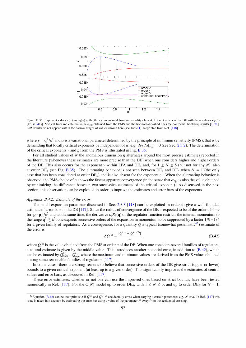
Figure B.35: Exponent values ν(α) and η(α) in the three-dimensional Ising universality class at different orders of the DE with the regulator Ek(q)[Eq. (B.41)]. Vertical lines indicate the value αopt obtained from the PMS and the horizontal dashed lines the conformal bootstrap results [1371].LPA results do not appear within the narrow ranges of values chosen here (see Table 1). Reprinted from Ref. [118].
where y = q2/k2 and α is a variational parameter determined by the principle of minimum sensitivity (PMS), that is bydemanding that locally critical exponents be independent of α, e.g. dν/dα|αopt = 0 (see Sec. 2.3.2). The determinationof the critical exponents ν and η from the PMS is illustrated in Fig. B.35.
For all studied values of N the anomalous dimension η alternates around the most precise estimates reported inthe literature (whenever these estimates are more precise than the DE) when one considers higher and higher ordersof the DE. This also occurs for the exponent ν within LPA and DE2 and, for 1 ≤ N ≤ 5 (but not for any N), alsoat order DE4 (see Fig. B.35). The alternating behavior is not seen between DE4 and DE6 when N = 1 (the onlycase that has been considered at order DE6) and is also absent for the exponent ω. When the alternating behavior isobserved, the PMS choice of α shows the fastest apparent convergence (in the sense that αopt is also the value obtainedby minimizing the difference between two successive estimates of the critical exponent). As discussed in the nextsection, this observation can be exploited in order to improve the estimates and error bars of the exponents.
Appendix B.4.2. Estimate of the errorThe small expansion parameter discussed in Sec. 2.3.3 [118] can be exploited in order to give a well-founded
estimate of error bars in the DE [117]. Since the radius of convergence of the DE is expected to be of the order of 4−9for |pi ·p j|/k2 and, at the same time, the derivative ∂tRk(q) of the regulator function restricts the internal momentum tothe range q2 . k2, one expects successive orders of the expansion in momentum to be suppressed by a factor 1/9−1/4for a given family of regulators. As a consequence, for a quantity Q a typical (somewhat pessimistic62) estimate ofthe error is
∆Q(s) =|Q(s) − Q(s−2)|
4, (B.42)
where Q(s) is the value obtained from the PMS at order s of the DE. When one considers several families of regulators,a natural estimate is given by the middle value. This introduces another potential error, in addition to (B.42), whichcan be estimated by Q(s)
max −Q(s)min where the maximum and minimum values are derived from the PMS values obtained
among some reasonable families of regulators [117].In some cases, there are strong reasons to believe that successive orders of the DE give strict (upper or lower)
bounds to a given critical exponent (at least up to a given order). This significantly improves the estimates of centralvalues and error bars, as discussed in Ref. [117].
These error estimates, whether or not one can use the improved ones based on strict bounds, have been testednumerically in Ref. [117]. For the O(N) model up to order DE4, with 1 ≤ N ≤ 5, and up to order DE6 for N = 1,
62Equation (B.42) can be too optimistic if Q(s) and Q(s−2) accidentally cross when varying a certain parameter, e.g. N or d. In Ref. [117] thisissue is taken into account by estimating the error bar using a value of the parameter N away from the accidental crossing.
92

the obtained values of the critical exponents, when compared with the most precise results available in the literature(when the latter are more precise than the DE), are always within the estimated error bars.
Appendix B.5. Fourth- and sixth-order of the derivative expansion
The DE has been pushed to fourth order for the O(N) model with 0 ≤ N ≤ 4 [117] and to sixth order for the Z2(Ising) universality class [118]. The “strict” DE has been used since it keeps equations to a more manageable size.The corresponding ansatz for the effective action reads
Γ∂4
k [φ] =
ˆr
{Uk(ρ) +
12
Zk(ρ)(∂µφ
a)2+
14
Yk(ρ)(∂µρ
)2+
W1,k(ρ)2
(∂µ∂νφ
a)2+
W2,k(ρ)2
(φa∂µ∂νφ
a)2
+ W3,k(ρ)∂µρ∂νφa∂µ∂νφa +
W4,k(ρ)2
φb∂µφa∂νφ
a∂µ∂νφb +
W5,k(ρ)2
ϕa∂µρ∂νρ∂µ∂νφa +
W6,k(ρ)4
((∂µφ
a)2)2
+W7,k(ρ)
4(∂µφ
a∂νφa)2
+W8,k(ρ)
2∂µφ
a∂νφa∂µρ∂νρ +
W9,k(ρ)2
(∂µφ
a)2(∂νρ
)2+
W10,k(ρ)4
((∂µρ
)2)2}
(B.43)
to fourth order [117], and
Γ∂6,Z2k [φ] =
ˆr
{Uk(φ) + 1
2 Zk(φ)(∂µφ)2 + 12 Wa
k (φ)(∂µ∂νφ)2 + 12φWb
k (φ)(∂2φ)(∂µφ)2 + 12 Wc
k (φ)((∂µφ)2
)2
+ 12 Xa
k (φ)(∂µ∂ν∂ρφ)2 + 12φXb
k (φ)(∂µ∂νφ)(∂ν∂ρφ)(∂µ∂ρφ) + 12φXc
k(φ)(∂2φ
)3+ 1
2 Xdk (φ)
(∂2φ
)2(∂µφ)2
+ 12 Xe
k(φ)(∂νφ)2(∂µφ)(∂2∂µφ) + 12 X f
k (φ)(∂ρφ)2(∂µ∂νφ)2 + 12φXg
k (φ)(∂2φ
) ((∂µφ)2
)2+ 1
96 Xhk (φ)
((∂µφ)2
)3}
(B.44)
to sixth order [118].
References
[1] E. C. G. Stueckelberg de Breidenbach, A. Petermann, Normalization of constants in the quanta theory, Helv. Phys. Acta 26 (1953) 499–520.doi:10.5169/seals-112426.
[2] M. Gell-Mann, F. Low, Quantum electrodynamics at small distances, Phys. Rev. 95 (1954) 1300–1312. doi:10.1103/PhysRev.95.
1300.[3] N. Bogolyubov, D. Shirkov, QUANTUM FIELDS, 1983.[4] K. Symanzik, Small distance behavior in field theory and power counting, Commun. Math. Phys. 18 (1970) 227–246. doi:10.1007/
BF01649434.[5] J. Callan, Curtis G., Broken scale invariance in scalar field theory, Phys. Rev. D 2 (1970) 1541–1547. doi:10.1103/PhysRevD.2.1541.[6] L. P. Kadanoff, Scaling laws for ising models near Tc, Physics 2 (1966) 263–272. doi:10.1103/PhysicsPhysiqueFizika.2.263.[7] K. G. Wilson, Renormalization Group and Critical Phenomena. I. Renormalization Group and the Kadanoff Scaling Picture, Phys. Rev. B
4 (1971) 3174–3183. doi:10.1103/PhysRevB.4.3174.[8] K. G. Wilson, Renormalization Group and Critical Phenomena. II. Phase-Space Cell Analysis of Critical Behavior, Phys. Rev. B 4 (1971)
3184–3205. doi:10.1103/PhysRevB.4.3184.[9] K. G. Wilson, J. B. Kogut, The renormalization group and the ε expansion, Phys. Rep. 12 (1974) 75. doi:doi:10.1016/0370-1573(74)
90023-4.[10] F. J. Wegner, A. Houghton, Renormalization Group Equation for Critical Phenomena, Phys. Rev. A 8 (1973) 401–412. doi:10.1103/
PhysRevA.8.401.[11] J. Polchinski, Renormalization and effective Lagrangians, Nucl. Phys. B 231 (1984) 269. doi:doi:10.1016/0550-3213(84)90287-6.[12] M. Fisher, Renormalization group theory: Its basis and formulation in statistical physics, Rev. Mod. Phys. 70 (1998) 653–681. doi:
10.1103/RevModPhys.70.653.[13] C. Bagnuls, C. Bervillier, Exact renormalization equations: an introductory review, Phys. Rep. 348 (2001) 91. doi:doi:10.1016/
S0370-1573(00)00137-X.[14] R. Guida, J. Zinn-Justin, Critical exponents of the N-vector model, J. Phys. A 31 (40) (1998) 8103. doi:doi:10.1088/0305-4470/31/
40/006.[15] A. Pelissetto, E. Vicari, Critical phenomena and renormalization-group theory, Phys. Rep. 368 (2002) 549. doi:http://dx.doi.org/
10.1016/S0370-1573(02)00219-3.[16] K. Gawedzki, A. Kupiainen, Massless lattice ϕ4
4 theory: Rigorous control of a renormalizable asymptotically free model, Communicationsin Mathematical Physics 99 (2) (1985) 197–252. doi:10.1007/BF01212281.
[17] T. Balaban, Convergent Renormalization Expansions for Lattice Gauge Theories, Commun. Math. Phys. 119 (1988) 243–285. doi:
10.1007/BF01217741.
93

[18] D. C. Brydges, T. Kennedy, Mayer expansions and the hamilton-jacobi equation, Journal of Statistical Physics 48 (1) (1987) 19–49.doi:10.1007/BF01010398.
[19] J. Feldman, J. Magnen, V. Rivasseau, R. Seneor, Construction and Borel Summability of Infrared φ4 in Four-dimensions by a Phase SpaceExpansion, Commun. Math. Phys. 109 (1987) 437–480. doi:10.1007/BF01206146.
[20] V. Rivasseau, From perturbative to constructive renormalization, 2nd Edition, Princeton Series in Physics, Princeton Univ Pr, 1991.[21] K. G. Wilson, The Renormalization Group: Critical Phenomena and the Kondo Problem, Rev. Mod. Phys. 47 (1975) 773. doi:10.1103/
RevModPhys.47.773.[22] U. Schollwock, The density-matrix renormalization group, Rev. Mod. Phys. 77 (2005) 259–315. arXiv:cond-mat/0409292, doi:
10.1103/RevModPhys.77.259.[23] K. G. Wilson, M. E. Fisher, Critical Exponents in 3.99 Dimensions, Phys. Rev. Lett. 28 (1972) 240–243. doi:10.1103/PhysRevLett.
28.240.[24] A. A. Migdal, Phase transitions in gauge and spin-lattice systems, JETP 42 (1975) 743.[25] A. M. Polyakov, Interaction of goldstone particles in two dimensions. Applications to ferromagnets and massive Yang-Mills fields, Phys.
Lett. B 59 (1975) 79. doi:http://dx.doi.org/10.1016/0370-2693(75)90161-6.[26] E. Brezin, J. Zinn-Justin, Renormalization of the Nonlinear σ Model in 2 + ε Dimensions—Application to the Heisenberg Ferromagnets,
Phys. Rev. Lett. 36 (1976) 691. doi:10.1103/PhysRevLett.36.691.[27] E. Brezin, J. Zinn-Justin, Spontaneous breakdown of continuous symmetries near two dimensions, Phys. Rev. B 14 (7) (1976) 3110.
doi:10.1103/PhysRevB.14.3110.[28] D. R. Nelson, R. A. Pelcovits, Momentum-shell recursion relations, anisotropic spins, and liquid crystals in 2 + ε dimensions, Phys. Rev.
B 16 (1977) 2191. doi:10.1103/PhysRevB.16.2191.[29] M. Moshe, J. Zinn-Justin, Quantum field theory in the large N limit: a review, Phys. Rep. 385 (2003) 69. doi:https://doi.org/10.
1016/S0370-1573(03)00263-1.[30] V. L. Berezinskii, Destruction of long-range order in one-dimensional and two-dimensional systems having a continuous symmetry group
i. classical systems, Sov. Phys. JETP 32 (1971) 493.URL http://www.jetp.ac.ru/cgi-bin/e/index/e/32/3/p493?a=list
[31] V. L. Berezinskii, Destruction of long-range order in one-dimensional and two-dimensional systems possessing a continuous symmetrygroup. ii. quantum systems, Sov. Phys. JETP 34 (1972) 610.URL http://www.jetp.ac.ru/cgi-bin/e/index/e/34/3/p610?a=list
[32] J. M. Kosterlitz, D. J. Thouless, Ordering, metastability and phase transitions in two-dimensional systems, J. of Phys. C 6 (1973) 1181.doi:doi:10.1088/0022-3719/6/7/010.
[33] J. M. Kosterlitz, D. J. Thouless, The critical properties of the two-dimensional XY model, J. Phys. C 7 (1974) 1046. doi:doi:10.1088/0022-3719/7/6/005.
[34] P. M. Chaikin, T. C. Lubensky, Principles of Condensed Matter Physics, Cambridge University Press, 1995.[35] A. Hasenfratz, P. Hasenfratz, Renormalization group study of scalar field theories, Nucl. Phys. B 270 (1986) 687–701. doi:https:
//doi.org/10.1016/0550-3213(86)90573-0.[36] T. Chang, D. Vvedensky, J. Nicoll, Differential renormalization-group generators for static and dynamic critical phenomena, Phys. Rep.
217 (1992) 279 – 360. doi:https://doi.org/10.1016/0370-1573(92)90041-W.URL http://www.sciencedirect.com/science/article/pii/037015739290041W
[37] A. Parola, L. Reatto, Liquid state theory and critical phenomena, Adv. Phys. 44 (1995) 211. doi:10.1080/00018739500101536.[38] J. F. Nicoll, T. S. Chang, H. E. Stanley, Approximate Renormalization Group Based on the Wegner-Houghton Differential Generator, Phys.
Rev. Lett. 33 (1974) 540. doi:10.1103/PhysRevLett.33.540.[39] J. Nicoll, T. Chang, An exact one-particle-irreducible renormalization-group generator for critical phenomena, Phys. Lett. A 62 (5) (1977)
287 – 289. doi:https://doi.org/10.1016/0375-9601(77)90417-0.[40] A. Parola, L. Reatto, Liquid-State Theory for Critical Phenomena, Phys. Rev. Lett. 53 (1984) 2417. doi:10.1103/PhysRevLett.53.
2417.[41] J. F. Nicoll, T. S. Chang, H. E. Stanley, Exact and approximate differential renormalization-group generators, Phys. Rev. A 13 (1976)
1251–1264. doi:10.1103/PhysRevA.13.1251.[42] K. E. Newman, E. K. Riedel, Critical exponents by the scaling-field method: The isotropic n-vector model in three dimensions, Phys. Rev.
B 30 (1984) 6615–6638. doi:10.1103/PhysRevB.30.6615.[43] K. E. Newman, E. K. Riedel, S. Muto, q-state potts model by wilson’s exact renormalization-group equation, Phys. Rev. B 29 (1984)
302–313. doi:10.1103/PhysRevB.29.302.[44] G. R. Golner, Nonperturbative renormalization-group calculations for continuum spin systems, Phys. Rev. B 33 (1986) 7863–7866. doi:
10.1103/PhysRevB.33.7863.[45] P. Hasenfratz, J. Nager, The cut-off dependence of the Higgs meson mass and the onset of new physics in the standard model, Z. Phys. C
37 (1988) 477–487. doi:10.1007/BF01578143.[46] G. Zumbach, Almost second order phase transitions, Phys. Rev. Lett. 71 (1993) 2421–2424. doi:10.1103/PhysRevLett.71.2421.[47] G. Zumbach, Phase transitions with O(n) symmetry broken down to O(n-p), Nucl. Phys. B 413 (1994) 771–791. doi:http://dx.doi.
org/10.1016/0550-3213(94)90012-4.[48] G. Zumbach, The local potential approximation of the renormalization group and its applications, Phys. Lett. A 190 (1994) 225–230.
doi:http://dx.doi.org/10.1016/0375-9601(94)90746-3.[49] D. S. Fisher, Random fields, random anisotropies, nonlinear σ models, and dimensional reduction, Phys. Rev. B 31 (1985) 7233. doi:
10.1103/PhysRevB.31.7233.[50] O. Narayan, D. S. Fisher, Dynamics of sliding charge-density waves in 4-ε dimensions, Phys. Rev. Lett. 68 (1992) 3615. doi:10.1103/
PhysRevLett.68.3615.[51] T. Nattermann, S. Stepanow, L.-H. Tang, H. Leschhorn, Dynamics of interface depinning in a disordered medium, J. Phys. II France 2 (8)
94

(1992) 1483. doi:10.1051/jp2:1992214.[52] P. Chauve, P. L. Doussal, K. J. Wiese, Renormalization of Pinned Elastic Systems: How Does It Work Beyond One Loop?, Phys. Rev. Lett.
86 (9) (2001) 1785. doi:10.1103/physrevlett.86.1785.[53] P. Le Doussal, K. J. Wiese, P. Chauve, Functional renormalization group and the field theory of disordered elastic systems, Phys. Rev. E 69
(2004) 026112. doi:10.1103/PhysRevE.69.026112.[54] G. Tarjus, M. Tissier, Nonperturbative Functional Renormalization Group for Random-Field Models: The Way Out of Dimensional Re-
duction, Phys. Rev. Lett. 93 (2004) 267008. doi:10.1103/PhysRevLett.93.267008.[55] A. Ringwald, C. Wetterich, Average action for the N-component ϕ4 theory, Nucl. Phys. B 334 (1990) 506. doi:doi:10.1016/
0550-3213(90)90489-Z.[56] C. Wetterich, Average action and the renormalization group equations, Nucl. Phys. B 352 (1991) 529. doi:doi:10.1016/
0550-3213(91)90099-J.[57] C. Wetterich, The average action for scalar fields near phase transitions, Z. Phys. C 57 (1993) 451–469. doi:10.1007/BF01474340.[58] C. Wetterich, Improvement of the average action, Z. Phys. C 60 (1993) 461–469. doi:10.1007/BF01560044.[59] C. Wetterich, Exact evolution equation for the effective potential, Phys. Lett. B 301 (1993) 90. doi:doi:10.1016/0370-2693(93)
90726-X.[60] J. Berges, N. Tetradis, C. Wetterich, Non-perturbative renormalization flow in quantum field theory and statistical physics, Phys. Rep. 363
(2002) 223–386. arXiv:hep-ph/0005122, doi:10.1016/S0370-1573(01)00098-9.[61] U. Ellwanger, Flow equations for n point functions and bound states, Z. Phys. C 62 (1994) 503. doi:10.1007/BF01555911.[62] T. R. Morris, The exact renormalization group and approximate solutions, Int. J. Mod. Phys. A 09 (1994) 2411. doi:10.1142/
S0217751X94000972.[63] M. Bonini, M. D’Attanasio, G. Marchesini, Perturbative renormalization and infrared finiteness in the Wilson renormalization group: the
massless scalar case, Nucl. Phys. B 409 (1993) 441 – 464. doi:https://doi.org/10.1016/0550-3213(93)90588-G.[64] K. I. Aoki, Introduction to the non-perturbative renormalization group and its recent applications, Int. J. Mod. Phys. B 14 (2000) 1249.
doi:10.1142/S0217979200000923.[65] J. Polonyi, Lectures on the functional renormalization group method, Central Eur.J.Phys. 1 (2003) 1–71. arXiv:hep-th/0110026,
doi:10.2478/BF02475552.[66] B. Delamotte, D. Mouhanna, M. Tissier, Nonperturbative renormalization-group approach to frustrated magnets, Phys. Rev. B 69 (2004)
134413. doi:10.1103/PhysRevB.69.134413.[67] J. M. Pawlowski, Aspects of the functional renormalisation group, Annals Phys. 322 (2007) 2831–2915. arXiv:hep-th/0512261,
doi:10.1016/j.aop.2007.01.007.[68] O. J. Rosten, Fundamentals of the Exact Renormalization Group, Phys. Rept. 511 (2012) 177–272. arXiv:1003.1366, doi:10.1016/
j.physrep.2011.12.003.[69] P. Kopietz, L. Bartosch, F. Schutz, Introduction to the Functional Renormalization Group, Springer, Berlin, 2010. doi:10.1007/
978-3-642-05094-7.[70] J. Braun, Fermion Interactions and Universal Behavior in Strongly Interacting Theories, J.Phys. G39 (2012) 033001. arXiv:1108.4449,
doi:10.1088/0954-3899/39/3/033001.[71] B. Delamotte, An Introduction to the Nonperturbative Renormalization Group, in: A. Schwenk, J. Polonyi (Eds.), Renormalization Group
and Effective Field Theory Approaches to Many-Body Systems, Vol. 852 of Lecture Notes in Physics, Springer Berlin Heidelberg, 2012,pp. 49–132. doi:10.1007/978-3-642-27320-9_2.
[72] H. Gies, Introduction to the Functional RG and Applications to Gauge Theories, Springer Berlin Heidelberg, Berlin, Heidelberg, 2012, pp.287–348. doi:10.1007/978-3-642-27320-9_6.URL https://doi.org/10.1007/978-3-642-27320-9_6
[73] J. Zinn-Justin, Quantum Field Theory and Critical Phenomena, Fourth Edition, Clarendon Press, Oxford, 2002.[74] D. F. Litim, Optimized renormalization group flows, Phys. Rev. D 64 (2001) 105007. doi:10.1103/PhysRevD.64.105007.[75] T. R. Morris, Equivalence of local potential approximations, J. High Energy Phys. 07 (2005) 027. doi:10.1088/1126-6708/2005/07/
027.[76] T. Papenbrock, C. Wetterich, Two-loop results from improved one loop computations, Z. Phys. C 65 (1995) 519. doi:10.1007/
BF01556140.[77] M. Bonini, G. Marchesini, M. Simionato, Beta function and flowing couplings in the exact wilson renormalization group in yang-mills
theory, Nucl. Phys. B 483 (1997) 475 – 494. doi:https://doi.org/10.1016/S0550-3213(96)00571-8.[78] T. R. Morris, J. F. Tighe, Convergence of derivative expansions of the renormalization group, J. High Energy Phys. 08 (1999) 007. doi:
10.1088/1126-6708/1999/08/007.[79] P. Kopietz, Two loop beta function from the exact renormalization group, Nucl. Phys. B 595 (2001) 493–518. arXiv:hep-th/0007128,
doi:10.1016/S0550-3213(00)00680-5.[80] J. I. Latorre, T. R. Morris, Exact scheme independence, JHEP 11 (2000) 004. arXiv:hep-th/0008123, doi:10.1088/1126-6708/
2000/11/004.[81] J. I. Latorre, T. R. Morris, Scheme Independence as an Inherent Redundancy in Quantum Field Theory, Int. J. Mod. Phys. A16 (2001)
2071–2074, [,72(2002)]. arXiv:hep-th/0102037, doi:10.1142/S0217751X01004724.[82] S. Arnone, A. Gatti, T. R. Morris, Exact scheme independence at one loop, JHEP 05 (2002) 059. arXiv:hep-th/0201237, doi:
10.1088/1126-6708/2002/05/059.[83] S. Arnone, A. Gatti, T. R. Morris, O. J. Rosten, Exact scheme independence at two loops, Phys. Rev. D69 (2004) 065009. arXiv:
hep-th/0309242, doi:10.1103/PhysRevD.69.065009.[84] D. F. Litim, Scheme independence at first order phase transitions and the renormalization group, Phys.Lett. B393 (1997) 103–109. arXiv:
hep-th/9609040, doi:10.1016/S0370-2693(96)01613-9.[85] M. Pernici, M. Raciti, F. Riva, Hard - soft renormalization and the exact renormalization group, Nucl. Phys. B520 (1998) 469–492.
95

arXiv:hep-th/9710145, doi:10.1016/S0550-3213(98)00176-X.[86] U. Ellwanger, The Running gauge coupling in the exact renormalization group approach, Z. Phys. C76 (1997) 721–727. arXiv:hep-ph/
9702309, doi:10.1007/s002880050593.[87] M. Pernici, M. Raciti, Wilsonian flow and mass independent renormalization, Nucl. Phys. B531 (1998) 560–592. arXiv:hep-th/
9803212, doi:10.1016/S0550-3213(98)80007-2.[88] O. J. Rosten, Universality From Very General Nonperturbative Flow Equations in QCD, Phys. Lett. B645 (2007) 466–469. arXiv:
hep-th/0611323, doi:10.1016/j.physletb.2006.12.057.[89] A. Codello, M. Demmel, O. Zanusso, Scheme dependence and universality in the functional renormalization group, Phys. Rev. D90 (2)
(2014) 027701. arXiv:1310.7625, doi:10.1103/PhysRevD.90.027701.[90] D. Schnoerr, I. Boettcher, J. M. Pawlowski, C. Wetterich, Error estimates and specification parameters for functional renormalization ,
Ann. Phys. 334 (2013) 83–99. doi:http://dx.doi.org/10.1016/j.aop.2013.03.013.[91] M. Reuter, N. Tetradis, C. Wetterich, The large-N limit and the high-temperature phase transition for the φ4 theory, Nucl. Phys. B 401
(1993) 567–590. doi:10.1016/0550-3213(93)90314-F.[92] T. R. Morris, On truncations of the exact renormalization group , Phys. Lett. B 334 (1994) 355. doi:10.1016/0370-2693(94)90700-5.[93] N. Tetradis, C. Wetterich, Scale dependence of the average potential around the maximum in φ4 theory., Nucl. Phys. B 383 (1992) 197.
doi:doi:10.1016/0550-3213(92)90676-3.[94] N. Tetradis, D. Litim, Analytical solutions of exact renormalization group equations , Nucl. Phys. B 464 (1996) 492–511. doi:http:
//dx.doi.org/10.1016/0550-3213(95)00642-7.[95] M. Pelaez, N. Wschebor, Ordered phase of the O(N) model within the nonperturbative renormalization group, Phys. Rev. E 94 (2016)
042136. doi:10.1103/PhysRevE.94.042136.[96] D. F. Litim, J. M. Pawlowski, L. Vergara, Convexity of the effective action from functional flows (2006). arXiv:hep-th/0602140.[97] T. R. Morris, Derivative expansion of the exact renormalization group , Phys. Lett. B 329 (1994) 241. doi:http://dx.doi.org/10.
1016/0370-2693(94)90767-6.[98] R. D. Ball, P. E. Haagensen, J. I. Latorre, E. Moreno, Scheme independence and the exact renormalization group, Phys. Lett. B 347 (1995)
80. doi:doi:10.1016/0370-2693(95)00025-G.[99] J. Comellas, Polchinski equation, reparameterization invariance and the derivative e xpansion , Nucl. Phys. B 509 (1998) 662–686. doi:
http://dx.doi.org/10.1016/S0550-3213(97)00692-5.[100] T. R. Morris, M. D. Turner, Derivative expansion of the renormalization group in O(N) scalar field theory , Nucl. Phys. B 509 (1998)
637–661. doi:http://dx.doi.org/10.1016/S0550-3213(97)00640-8.[101] G. Zumbach, The renormalization group in the local potential approximation and its applications to the O (n) model, Nucl. Phys. B 413
(1994) 754 – 770. doi:http://dx.doi.org/10.1016/0550-3213(94)90011-6.[102] N. Defenu, P. Mati, I. G. Marian, I. Nandori, A. Trombettoni, Truncation effects in the functional renormalization group study of sponta-
neous symmetry breaking, J. High Energy Phys. 05 (2015) 141. doi:10.1007/JHEP05(2015)141.[103] N. D. Mermin, H. Wagner, Absence of Ferromagnetism or Antiferromagnetism in One- or Two-Dimensional Isotropic Heisenberg Models,
Phys. Rev. Lett. 17 (1966) 1133–1136. doi:10.1103/PhysRevLett.17.1133.[104] P. C. Hohenberg, Existence of long-range order in one and two dimensions, Phys. Rev. 158 (1967) 383–386. doi:10.1103/PhysRev.
158.383.[105] S. Coleman, There are no goldstone bosons in two dimensions, Commun. Math. Phys. 31 (1973) 259–264. doi:10.1007/BF01646487.[106] P. Labus, R. Percacci, G. P. Vacca, Asymptotic safety in O(N) scalar models coupled to gravity, Phys. Lett. B753 (2016) 274–281.
arXiv:1505.05393, doi:10.1016/j.physletb.2015.12.022.[107] B. Delamotte, M. Tissier, N. Wschebor, Scale invariance implies conformal invariance for the three-dimensional Ising model, Phys. Rev. E
93 (2016) 012144. doi:10.1103/PhysRevE.93.012144.[108] J.-P. Blaizot, R. Mendez-Galain, N. Wschebor, Nonperturbative renormalization group and momentum dependence of n-point functions. I,
Phys. Rev. E 74 (2006) 051116. doi:10.1103/PhysRevE.74.051116.[109] A. Codello, Scaling solutions in a continuous dimension, J. Phys. A: Math. Theor. 45 (2012) 465006. doi:10.1088/1751-8113/45/
46/465006.[110] A. Codello, G. D’Odorico, O(N)-Universality Classes and the Mermin-Wagner Theorem, Phys. Rev. Lett. 110 (2013) 141601. doi:
10.1103/PhysRevLett.110.141601.[111] A. Codello, N. Defenu, G. D’Odorico, Critical exponents of O(N) models in fractional dimensions, Phys. Rev. D 91 (2015) 105003.
doi:10.1103/PhysRevD.91.105003.[112] N. Tetradis, C. Wetterich, Critical exponents from the effective average action, Nucl. Phys. B 422 (1994) 541. doi:doi:10.1016/
0550-3213(94)90446-4.[113] K.-I. Aoki, K. Morikawa, W. Souma, J.-I. Sumi, H. Terao, Rapidly Converging Truncation Scheme of the Exact Renormalization Group,
Prog. Theor. Phys. 99 (1998) 451. doi:10.1143/PTP.99.451.[114] T. R. Morris, Three-dimensional massive scalar field theory and the derivative expansion of the renormalization group, Nucl. Phys. B 495
(1997) 477. doi:https://doi.org/10.1016/S0550-3213(97)00233-2.[115] S. Seide, C. Wetterich, Equation of state near the endpoint of the critical line, Nucl. Phys. B 562 (1999) 524–546. doi:http://dx.doi.
org/10.1016/S0550-3213(99)00545-3.[116] G. v. Gersdorff, C. Wetterich, Nonperturbative renormalization flow and essential scaling for the Kosterlitz-Thouless transition, Phys. Rev.
B 64 (2001) 054513. doi:10.1103/PhysRevB.64.054513.[117] G. De Polsi, I. Balog, M. Tissier, N. Wschebor, Precision calculation of critical exponents in the O(N) universality classes with the
nonperturbative renormalization group, Phys. Rev. E 101 (2020) 042113. doi:10.1103/PhysRevE.101.042113.[118] I. Balog, H. Chate, B. Delamotte, M. Marohnic, N. Wschebor, Convergence of nonperturbative approximations to the renormalization
group, Phys. Rev. Lett. 123 (2019) 240604. doi:10.1103/PhysRevLett.123.240604.[119] N. Hasselmann, Effective-average-action-based approach to correlation functions at finite momenta, Phys. Rev. E 86 (2012) 041118.
96

doi:10.1103/PhysRevE.86.041118.[120] F. Rose, N. Dupuis, Nonperturbative renormalization-group approach preserving the momentum dependence of correlation functions, Phys.
Rev. B 97 (2018) 174514. doi:10.1103/PhysRevB.97.174514.[121] F. Benitez, J.-P. Blaizot, H. Chate, B. Delamotte, R. Mendez-Galain, N. Wschebor, Solutions of renormalization group flow equations with
full momentum dependence, Phys. Rev. E 80 (2009) 030103(R). doi:10.1103/PhysRevE.80.030103.[122] F. Benitez, J.-P. Blaizot, H. Chate, B. Delamotte, R. Mendez-Galain, N. Wschebor, Nonperturbative renormalization group preserving
full-momentum dependence: Implementation and quantitative evaluation, Phys. Rev. E 85 (2012) 026707. doi:10.1103/PhysRevE.85.026707.
[123] M. Hasenbusch, Finite size scaling study of lattice models in the three-dimensional Ising universality class, Phys. Rev. B 82 (2010) 174433.doi:10.1103/PhysRevB.82.174433.
[124] M. Campostrini, M. Hasenbusch, A. Pelissetto, E. Vicari, Theoretical estimates of the critical exponents of the superfluid transition in 4Heby lattice methods, Phys. Rev. B 74 (2006) 144506. doi:10.1103/PhysRevB.74.144506.
[125] M. Campostrini, M. Hasenbusch, A. Pelissetto, P. Rossi, E. Vicari, Critical exponents and equation of state of the three-dimensionalHeisenberg universality class, Phys. Rev. B 65 (2002) 144520. doi:10.1103/PhysRevB.65.144520.
[126] M. Hasenbusch, Monte Carlo study of an improved clock model in three dimensions, Phys. Rev. B100 (22) (2019) 224517. arXiv:
1910.05916, doi:10.1103/PhysRevB.100.224517.[127] N. Clisby, B. Dunweg, High-precision estimate of the hydrodynamic radius for self-avoiding walks, Phys. Rev. E 94 (2016) 052102.
doi:10.1103/PhysRevE.94.052102.URL https://link.aps.org/doi/10.1103/PhysRevE.94.052102
[128] N. Clisby, Scale-free monte carlo method for calculating the critical exponent γ of self-avoiding walks, Journal of Physics A: Mathematicaland Theoretical 50 (26) (2017) 264003. doi:10.1088/1751-8121/aa7231.URL https://doi.org/10.1088%2F1751-8121%2Faa7231
[129] M. V. Kompaniets, E. Panzer, Minimally subtracted six loop renormalization of O(n)-symmetric φ4 theory and critical exponents, Phys.Rev. D96 (3) (2017) 036016. arXiv:1705.06483, doi:10.1103/PhysRevD.96.036016.
[130] H. Shimada, S. Hikami, Fractal dimensions of self-avoiding walks and Ising high-temperature graphs in 3D conformal bootstrap, J. Statist.Phys. 165 (2016) 1006. arXiv:1509.04039, doi:10.1007/s10955-016-1658-x.
[131] F. Kos, D. Poland, D. Simmons-Duffin, A. Vichi, Precision islands in the Ising and O(N) models, J. High Energy Phys. 08 (2016) 036.doi:10.1007/JHEP08(2016)036.
[132] D. Simmons-Duffin, The Lightcone Bootstrap and the Spectrum of the 3d Ising CFT, JHEP 03 (2017) 086. arXiv:1612.08471, doi:10.1007/JHEP03(2017)086.
[133] A. C. Echeverri, B. von Harling, M. Serone, The effective bootstrap, Journal of High Energy Physics 2016 (9) (2016) 97. doi:10.1007/JHEP09(2016)097.URL https://doi.org/10.1007/JHEP09(2016)097
[134] S. M. Chester, W. Landry, J. Liu, D. Poland, D. Simmons-Duffin, N. Su, A. Vichi, Carving out ope space and precise o(2) model criticalexponents (2019). arXiv:1912.03324.
[135] D. Litim, Optimisation of the exact renormalization group, Phys. Lett. B 486 (2000) 92. doi:http://dx.doi.org/10.1016/
S0370-2693(00)00748-6.[136] D. F. Litim, Mind the gap, Int. J. Mod. Phys. A 16 (2001) 2081–2087. doi:10.1142/S0217751X01004748.[137] D. F. Litim, Critical exponents from optimised renormalisation group flows, Nucl. Phys. B 631 (2002) 128–158. doi:https://doi.
org/10.1016/S0550-3213(02)00186-4.[138] D. F. Litim, Universality and the renormalisation group, J. High Energy Phys. 07 (2005) 005.
URL http://stacks.iop.org/1126-6708/2005/i=07/a=005
[139] S.-B. Liao, J. Polonyi, M. Strickland, Optimization of renormalization group flow, Nucl. Phys. B 567 (2000) 493–514. doi:https:
//doi.org/10.1016/S0550-3213(99)00496-4.[140] L. Canet, B. Delamotte, D. Mouhanna, J. Vidal, Optimization of the derivative expansion in the nonperturbative renormalization group,
Phys. Rev. D 67 (2003) 065004. doi:10.1103/PhysRevD.67.065004.[141] L. Canet, B. Delamotte, D. Mouhanna, J. Vidal, Nonperturbative renormalization group approach to the Ising model: A derivative expansion
at order ∂4 , Phys. Rev. B 68 (2003) 064421. doi:10.1103/PhysRevB.68.064421.[142] L. Canet, Optimization of field-dependent nonperturbative renormalization group flows, Phys. Rev. B71 (2005) 012418. arXiv:hep-th/
0409300, doi:10.1103/PhysRevB.71.012418.[143] I. Nandori, I. G. Marian, V. Bacso, Spontaneous symmetry breaking and optimization of functional renormalization group, Phys. Rev.
D89 (4) (2014) 047701. arXiv:1303.4508, doi:10.1103/PhysRevD.89.047701.[144] J. M. Pawlowski, M. M. Scherer, R. Schmidt, S. J. Wetzel, Physics and the choice of regulators in functional renormalisation group flows
(Dec. 2015). arXiv:1512.03598.[145] D. F. Litim, D. Zappala, Ising exponents from the functional renormalization group, Phys. Rev. D 83 (2011) 085009. doi:10.1103/
PhysRevD.83.085009.[146] T. R. Morris, The renormalization group and two-dimensional multicritical effective scalar field theory, Phys. Lett. B 345 (1995) 139–148.
doi:https://doi.org/10.1016/0370-2693(94)01603-A.[147] H. Ballhausen, J. Berges, C. Wetterich, Critical phenomena in continuous dimension, Phys. Lett. B 582 (2004) 144–150. doi:https:
//doi.org/10.1016/j.physletb.2003.12.033.[148] N. Defenu, A. Codello, Scaling solutions in the derivative expansion, Phys. Rev. D 98 (2018) 016013. doi:10.1103/PhysRevD.98.
016013.[149] M. D’Attanasio, T. R. Morris, Large N and the renormalization group, Phys. Lett. B 409 (1997) 363. doi:http://dx.doi.org/10.
1016/S0370-2693(97)00866-6.[150] S. Yabunaka, B. Delamotte, Surprises in o(n) models: Nonperturbative fixed points, large n limits, and multicriticality, Phys. Rev. Lett. 119
97

(2017) 191602. doi:10.1103/PhysRevLett.119.191602.[151] S. Yabunaka, B. Delamotte, Why might the standard large n analysis fail in the O(n) model: The role of cusps in fixed point potentials,
Phys. Rev. Lett. 121 (2018) 231601. doi:10.1103/PhysRevLett.121.231601.[152] A. Katsis, N. Tetradis, Multicritical points of the O(N) scalar theory in 2 < d < 4 for large N, Phys. Lett. B780 (2018) 491–494.
arXiv:1801.07659, doi:10.1016/j.physletb.2018.03.038.[153] M. Grater, C. Wetterich, Kosterlitz-Thouless Phase Transition in the Two Dimensional LinearσModel, Phys. Rev. Lett. 75 (1995) 378–381.
doi:10.1103/PhysRevLett.75.378.[154] P. Jakubczyk, N. Dupuis, B. Delamotte, Reexamination of the nonperturbative renormalization-group approach to the Kosterlitz-Thouless
transition, Phys. Rev. E 90 (2014) 062105. doi:10.1103/PhysRevE.90.062105.[155] P. Jakubczyk, A. Eberlein, Thermodynamics of the two-dimensional XY model from functional renormalization, Phys. Rev. E 93 (2016)
062145. doi:10.1103/PhysRevE.93.062145.[156] A. Rancon, N. Dupuis, Kosterlitz-Thouless signatures in the low-temperature phase of layered three-dimensional systems, Phys. Rev. B 96
(2017) 214512. doi:10.1103/PhysRevB.96.214512.[157] P. Jakubczyk, W. Metzner, Longitudinal fluctuations in the Berezinskii-Kosterlitz-Thouless phase, Phys. Rev. B 95 (2017) 085113. doi:
10.1103/PhysRevB.95.085113.[158] P. Jakubczyk, Renormalization theory for the Fulde-Ferrell-Larkin-Ovchinnikov states at T > 0, Phys. Rev. A95 (2017) 063626. arXiv:
1706.01524, doi:10.1103/PhysRevA.95.063626.[159] N. Defenu, A. Trombettoni, I. Nandori, T. Enss, Nonperturbative renormalization group treatment of amplitude fluctuations for ϕ4 topo-
logical phase transitions, Phys. Rev. B 96 (2017) 174505. doi:10.1103/PhysRevB.96.174505.[160] J. Krieg, P. Kopietz, Dual lattice functional renormalization group for the Berezinskii-Kosterlitz-Thouless transition: Irrelevance of ampli-
tude and out-of-plane fluctuations, Phys. Rev. E 96 (2017) 042107. doi:10.1103/PhysRevE.96.042107.[161] Villain, J., Theory of one- and two-dimensional magnets with an easy magnetization plane. ii. the planar, classical, two-dimensional
magnet, J. Phys. France 36 (1975) 581–590. doi:10.1051/jphys:01975003606058100.[162] C. S. Fischer, H. Gies, Renormalization flow of Yang-Mills propagators, JHEP 10 (2004) 048. arXiv:hep-ph/0408089, doi:10.1088/
1126-6708/2004/10/048.[163] J. Borchardt, B. Knorr, Solving functional flow equations with pseudospectral methods, Phys. Rev. D 94 (2016) 025027. doi:10.1103/
PhysRevD.94.025027.[164] J. Borchardt, B. Knorr, Global solutions of functional fixed point equations via pseudospectral methods, Phys. Rev. D 91 (2015) 105011.
doi:10.1103/PhysRevD.91.105011.[165] F. Rose, F. Benitez, F. Leonard, B. Delamotte, Bound states of the φ4 model via the nonperturbative renormalization group, Phys. Rev. D
93 (2016) 125018. doi:10.1103/PhysRevD.93.125018.[166] E. Grossi, N. Wink, Resolving phase transitions with Discontinuous Galerkin methods (3 2019). arXiv:1903.09503.[167] D. F. Litim, Derivative expansion and renormalisation group flows, J. High Energy Phys. 11 (2001) 059. doi:10.1088/1126-6708/
2001/11/059.[168] Yu. A. Kubyshin, R. Neves, R. Potting, Solutions of the polchinski erg equation in the O(n) scalar model, Int. J. Mod. Phys. A17 (2002)
4871. arXiv:hep-th/0202199, doi:10.1142/S0217751X02011400.[169] J. Berges, N. Tetradis, C. Wetterich, Critical Equation of State from the Average Action, Phys. Rev. Lett. 77 (1996) 873–876. doi:
10.1103/PhysRevLett.77.873.[170] A. Rancon, O. Kodio, N. Dupuis, P. Lecheminant, Thermodynamics in the vicinity of a relativistic quantum critical point in 2+1 dimensions,
Phys. Rev. E 88 (2013) 012113. doi:10.1103/PhysRevE.88.012113.[171] A. Rancon, N. Dupuis, Quantum XY criticality in a two-dimensional Bose gas near the Mott transition, Europhys. Lett. 104 (2013) 16002.
doi:10.1209/0295-5075/104/16002.[172] A. Rancon, L.-P. Henry, F. Rose, D. L. Cardozo, N. Dupuis, P. C. W. Holdsworth, T. Roscilde, Critical Casimir forces from the equation of
state of quantum critical systems, Phys. Rev. B 94 (2016) 140506(R). doi:10.1103/PhysRevB.94.140506.[173] N. Dupuis, Infrared behavior in systems with a broken continuous symmetry: Classical O(N) model versus interacting bosons, Phys. Rev.
E 83 (2011) 031120. doi:10.1103/PhysRevE.83.031120.[174] J.-M. Caillol, The non-perturbative renormalization group in the ordered phase, Nucl. Phys. B 855 (2012) 854. doi:10.1016/j.
nuclphysb.2011.10.026.[175] A. Z. Patasinskij, V. L. Pokrovskij, Longitudinal susceptibility and correlations in degenerate systems, Sov. Phys. JETP 37 (1973) 733, zh.
Eksp. Teor. Fiz. 64, 1445 (1973).[176] W. Zwerger, Anomalous Fluctuations in Phases with a Broken Continuous Symmetry, Phys. Rev. Lett. 92 (2004) 027203. doi:10.1103/
PhysRevLett.92.027203.[177] T. Hellwig, A. Wipf, O. Zanusso, Scaling and superscaling solutions from the functional renormalization group, Phys. Rev. D92 (8) (2015)
085027. arXiv:1508.02547, doi:10.1103/PhysRevD.92.085027.[178] A. Eichhorn, D. Mesterhazy, M. M. Scherer, Multicritical behavior in models with two competing order parameters, Phys. Rev. E 88 (2013)
042141. arXiv:1306.2952, doi:10.1103/PhysRevE.88.042141.[179] A. Codello, M. Safari, G. P. Vacca, O. Zanusso, Functional perturbative RG and CFT data in the ε-expansion, Eur. Phys. J. C78 (1) (2018)
30. arXiv:1705.05558, doi:10.1140/epjc/s10052-017-5505-2.[180] D. F. Litim, E. Marchais, P. Mati, Fixed points and the spontaneous breaking of scale invariance, Phys. Rev. D95 (12) (2017) 125006.
arXiv:1702.05749, doi:10.1103/PhysRevD.95.125006.[181] A. Eichhorn, L. Janssen, M. M. Scherer, Critical o(n) models above four dimensions: Small-n solutions and stability, Phys. Rev. D 93
(2016) 125021. doi:10.1103/PhysRevD.93.125021.[182] R. Percacci, G. P. Vacca, Are there scaling solutions in the O(N)-models for large N in d > 4 ?, Phys. Rev. D90 (2014) 107702. arXiv:
1405.6622, doi:10.1103/PhysRevD.90.107702.[183] P. Mati, Vanishing beta function curves from the functional renormalization group, Phys. Rev. D91 (12) (2015) 125038. arXiv:1501.
98

00211, doi:10.1103/PhysRevD.91.125038.[184] N. Defenu, A. Trombettoni, A. Codello, Fixed-point structure and effective fractional dimensionality for O(N) models with long-range
interactions, Phys. Rev. E92 (5) (2015) 052113. arXiv:1409.8322, doi:10.1103/PhysRevE.92.052113.[185] N. Defenu, A. Trombettoni, S. Ruffo, Criticality and phase diagram of quantum long-range O( N ) models, Phys. Rev. B96 (10) (2017)
104432. arXiv:1704.00528, doi:10.1103/PhysRevB.96.104432.[186] R. Goll, P. Kopietz, Renormalization group for ϕ4-theory with long-range interaction and the critical exponent η of the Ising model, Phys.
Rev. E98 (2) (2018) 022135. arXiv:1804.04150, doi:10.1103/PhysRevE.98.022135.[187] N. Defenu, A. Codello, S. Ruffo, A. Trombettoni, Criticality of spin systems with weak long-range interactions, J. Phys. A 53 (14) (2020)
143001. arXiv:1908.05158, doi:10.1088/1751-8121/ab6a6c.[188] D. F. Litim, E. Marchais, Critical O(N) models in the complex field plane, Phys. Rev. D95 (2) (2017) 025026. arXiv:1607.02030,
doi:10.1103/PhysRevD.95.025026.[189] A. Juttner, D. F. Litim, E. Marchais, Global Wilson-Fisher fixed points, Nucl. Phys. B921 (2017) 769–795. arXiv:1701.05168, doi:
10.1016/j.nuclphysb.2017.06.010.[190] K. Halpern, K. Huang, Fixed-Point Structure of Scalar Fields, Phys. Rev. Lett. 74 (1995) 3526–3529. doi:10.1103/PhysRevLett.74.
3526.URL https://link.aps.org/doi/10.1103/PhysRevLett.74.3526
[191] K. Halpern, K. Huang, Halpern and Huang Reply:, Phys. Rev. Lett. 77 (1996) 1659–1659. doi:10.1103/PhysRevLett.77.1659.URL https://link.aps.org/doi/10.1103/PhysRevLett.77.1659
[192] T. R. Morris, On the fixed point structure of scalar fields, Phys. Rev. Lett. 77 (1996) 1658. arXiv:hep-th/9601128, doi:10.1103/PhysRevLett.77.1658.
[193] H. Gies, Flow equation for Halpern-Huang directions of scalar O(N) models, Phys. Rev. D63 (2001) 065011. arXiv:hep-th/0009041,doi:10.1103/PhysRevD.63.065011.
[194] I. Hamzaan Bridle, T. R. Morris, Fate of nonpolynomial interactions in scalar field theory, Phys. Rev. D94 (2016) 065040. arXiv:
1605.06075, doi:10.1103/PhysRevD.94.065040.[195] P. Jakubczyk, M. Napiorkowski, Critical Casimir forces for O(N) models from functional renormalization, Phys.Rev. B87 (2013) 165439.
arXiv:1212.2647, doi:10.1103/PhysRevB.87.165439.[196] A. Codello, R. Percacci, Fixed Points of Nonlinear Sigma Models in d>2, Phys. Lett. B672 (2009) 280–283. arXiv:0810.0715, doi:
10.1016/j.physletb.2009.01.032.[197] R. Flore, A. Wipf, O. Zanusso, Functional renormalization group of the non-linear sigma model and the O(N) universality class, Phys. Rev.
D87 (6) (2013) 065019. arXiv:1207.4499, doi:10.1103/PhysRevD.87.065019.[198] R. Percacci, M. Safari, Functional renormalization of N scalars with O(N) invariance, Phys. Rev. D88 (2013) 085007. arXiv:1306.3918,
doi:10.1103/PhysRevD.88.085007.[199] R. B. A. Zinati, A. Codello, Functional rg approach to the potts model, J. Stat. Mech: Theory Exp. 2018 (2018) 013206. doi:10.1088/
1742-5468/aa9dcc.[200] S. Nagy, I. Nandori, J. Polonyi, K. Sailer, Functional Renormalization Group Approach to the Sine-Gordon Model, Phys. Rev. Lett. 102
(2009) 241603. doi:10.1103/PhysRevLett.102.241603.[201] V. Pangon, Structure of the broken phase of the sine-Gordon model using functional renormalisation, Int. J. Mod. Phys. A 27 (2012)
1250014. doi:10.1142/S0217751X12500145.[202] V. Pangon, Generating the mass gap of the sine-Gordon model (Nov. 2011). arXiv:1111.6425.[203] V. Bacso, N. Defenu, A. Trombettoni, I. Nandori, c-function and central charge of the sine-Gordon model from the non-perturbative
renormalization group flow , Nucl. Phys. B 901 (2015) 444 – 460. doi:http://dx.doi.org/10.1016/j.nuclphysb.2015.11.001.[204] P. Oak, B. Sathiapalan, Exact renormalization group and sine gordon theory, J. High Energy Phys. 2017 (7) (2017) 103. doi:10.1007/
JHEP07(2017)103.[205] R. Daviet, N. Dupuis, Nonperturbative functional renormalization-group approach to the sine-Gordon model and the Lukyanov-
Zamolodchikov conjecture, Phys. Rev. Lett. 122 (2019) 155301. doi:10.1103/PhysRevLett.122.155301.[206] S. Lukyanov, A. B. Zamolodchikov, Exact expectation values of local fields in the quantum sine-Gordon model, Nucl. Phys. B 493 (3)
(1997) 571. doi:https://doi.org/10.1016/S0550-3213(97)00123-5.[207] J.-P. Blaizot, R. Mendez-Galain, N. Wschebor, Non perturbative renormalization group, momentum dependence of n-point functions
and the transition temperature of the weakly interacting Bose gas, Europhys.Lett. 72 (2005) 705–711. arXiv:cond-mat/0412481,doi:10.1209/epl/i2005-10318-5.
[208] J.-P. Blaizot, R. Mendez-Galain, N. Wschebor, Nonperturbative renormalization group and momentum dependence of n-point functions.II, Phys. Rev. E 74 (2006) 051117. doi:10.1103/PhysRevE.74.051117.
[209] J.-P. Blaizot, R. Mendez-Galain, N. Wschebor, Non-perturbative renormalization group calculation of the scalar self-energy, Eur. Phys. J.B 58 (2007) 297. doi:10.1140/epjb/e2007-00223-3.
[210] S. Ledowski, N. Hasselmann, P. Kopietz, Self-energy and critical temperature of weakly interacting bosons, Phys. Rev. A 69 (2004)061601. doi:10.1103/PhysRevA.69.061601.
[211] N. Hasselmann, A. Sinner, P. Kopietz, Two-parameter scaling of correlation functions near continuous phase transitions, Phys. Rev. E 76(2007) 040101. doi:10.1103/PhysRevE.76.040101.
[212] A. Sinner, N. Hasselmann, P. Kopietz, Functional renormalization group in the broken symmetry phase: momentum dependence andtwo-parameter scaling of the self-energy, J. Phys.: Condens. Matter 20 (2008) 075208. doi:10.1088/0953-8984/20/7/075208.
[213] D. Guerra, R. Mendez-Galain, N. Wschebor, Correlation functions in the non perturbative renormalization group and field expansion, Eur.Phys. J. B 59 (2007) 357. doi:DOI:10.1140/epjb/e2007-00296-x.
[214] N. Hasselmann, F. L. Braghin, Nonlocal effective-average-action approach to crystalline phantom membranes, Phys. Rev. E 83 (2011)031137. doi:10.1103/PhysRevE.83.031137.
[215] S. Mathey, T. Gasenzer, J. M. Pawlowski, Anomalous scaling at nonthermal fixed points of Burgers’ and gross-pitaevskii turbulence, Phys.
99

Rev. A 92 (2015) 023635. doi:10.1103/PhysRevA.92.023635.URL http://link.aps.org/doi/10.1103/PhysRevA.92.023635
[216] L. Canet, H. Chate, B. Delamotte, General framework of the non-perturbative renormalization group for non-equilibrium steady states,Journal of Physics A: Mathematical and Theoretical 44 (49) (2011) 495001. doi:10.1088/1751-8113/44/49/495001.URL https://doi.org/10.1088%2F1751-8113%2F44%2F49%2F495001
[217] L. Canet, B. Delamotte, N. Wschebor, Fully developed isotropic turbulence: Nonperturbative renormalization group formalism and fixed-point solution, Phys. Rev. E 93 (2016) 063101. doi:10.1103/PhysRevE.93.063101.URL http://link.aps.org/doi/10.1103/PhysRevE.93.063101
[218] P. Feldmann, A. Wipf, L. Zambelli, Critical Wess-Zumino models with four supercharges in the functional renormalization group approach,Phys. Rev. D98 (9) (2018) 096005. arXiv:1712.03910, doi:10.1103/PhysRevD.98.096005.
[219] J.-P. Blaizot, R. Mendez-Galain, N. Wschebor, A new method to solve the non-perturbative renormalization group equations, Phys. Lett.B 632 (2006) 571. doi:10.1016/j.physletb.2005.10.086.
[220] F. Benitez, R. Mendez-Galain, N. Wschebor, Calculations on the two-point function of the O(N) model, Phys. Rev. B 77 (2008) 024431.doi:10.1103/PhysRevB.77.024431.
[221] F. Rose, F. Leonard, N. Dupuis, Higgs amplitude mode in the vicinity of a (2 + 1)-dimensional quantum critical point: A nonperturbativerenormalization-group approach, Phys. Rev. B 91 (2015) 224501. doi:10.1103/PhysRevB.91.224501.
[222] A. A. Pogorelov, I. M. Suslov, Renormalization group functions for two-dimensional phase transitions: To the problem of singular contri-butions, J. Exp. Theor. Phys. 105 (2007) 360–370. doi:10.1134/S1063776107080080.
[223] N. Dupuis, K. Sengupta, Non-perturbative renormalization-group approach to lattice models, Eur. Phys. J. B 66 (2008) 271. doi:10.
1140/epjb/e2008-00417-1.[224] T. Machado, N. Dupuis, From local to critical fluctuations in lattice models: A nonperturbative renormalization-group approach, Phys.
Rev. E 82 (2010) 041128. doi:10.1103/PhysRevE.82.041128.[225] J.-M. Caillol, Critical line of the theory on a simple cubic lattice in the local potential approximation , Nucl. Phys. B 865 (2012) 291.
doi:http://dx.doi.org/10.1016/j.nuclphysb.2012.07.032.[226] J.-M. Caillol, Critical line of the Φ4 scalar field theory on a 4D cubic lattice in the local potential approximation, Condens. Matter Phys.
16 (2013) 43005. doi:10.5488/CMP.16.43005.[227] R. Banerjee, M. Niedermaier, Graph rules for the linked cluster expansion of the Legendre effective action, J. Math. Phys. 60 (1) (2019)
013504. arXiv:1812.06602, doi:10.1063/1.5031429.[228] R. Banerjee, Critical behavior of the hopping expansion from the Functional Renormalization Group, PoS LATTICE2018 (2018) 249.
arXiv:1812.02251, doi:10.22323/1.334.0249.[229] A. Rancon, Nonperturbative renormalization group approach to quantum XY spin models, Phys. Rev. B 89 (2014) 214418. doi:10.1103/
PhysRevB.89.214418.[230] J. Krieg, P. Kopietz, Exact renormalization group for quantum spin systems, Phys. Rev. B 99 (2019) 060403. doi:10.1103/PhysRevB.
99.060403.URL https://link.aps.org/doi/10.1103/PhysRevB.99.060403
[231] A. Rancon, N. Dupuis, Nonperturbative renormalization group approach to the Bose-Hubbard model, Phys. Rev. B 83 (2011) 172501.doi:10.1103/PhysRevB.83.172501.
[232] A. Rancon, N. Dupuis, Nonperturbative renormalization group approach to strongly correlated lattice bosons, Phys. Rev. B 84 (2011)174513. doi:10.1103/PhysRevB.84.174513.
[233] A. Rancon, N. Dupuis, Quantum criticality of a Bose gas in an optical lattice near the Mott transition, Phys. Rev. A 85 (2012) 011602(R).doi:10.1103/PhysRevA.85.011602.
[234] A. Rancon, N. Dupuis, Thermodynamics of a Bose gas near the superfluid–Mott-insulator transition, Phys. Rev. A 86 (2012) 043624.doi:10.1103/PhysRevA.86.043624.
[235] J. Reuther, R. Thomale, Cluster functional renormalization group, Phys. Rev. B 89 (2014) 024412. doi:10.1103/PhysRevB.89.024412.[236] N. Wentzell, C. Taranto, A. Katanin, A. Toschi, S. Andergassen, Correlated starting points for the functional renormalization group, Phys.
Rev. B 91 (2015) 045120. doi:10.1103/PhysRevB.91.045120.[237] C. Taranto, S. Andergassen, J. Bauer, K. Held, A. Katanin, W. Metzner, G. Rohringer, A. Toschi, From Infinite to Two Dimensions through
the Functional Renormalization Group, Phys. Rev. Lett. 112 (2014) 196402. doi:10.1103/PhysRevLett.112.196402.[238] S. Sachdev, Quantum Phase Transitions, 2nd Edition, Cambridge University Press, Cambridge, England, 2011.[239] N. Tetradis, C. Wetterich, The high temperature phase transition for φ4 theories, Nucl. Phys. B 398 (1993) 659–696. doi:10.1016/
0550-3213(93)90608-R.[240] D. F. Litim, J. M. Pawlowski, Non-perturbative thermal flows and resummations, J. High Energy Phys. 11 (2006) 026. doi:10.1088/
1126-6708/2006/11/026.[241] L. Schlessinger, Use of analyticity in the calculation of nonrelativistic scattering amplitudes, Phys. Rev. 167 (1968) 1411. doi:10.1103/
PhysRev.167.1411.[242] H. J. Vidberg, J. W. Serene, Solving the Eliashberg equations by means of N-point Pade approximants, J. Low Temp. Phys. 29 (1977) 179.
doi:10.1007/BF00655090.[243] R.-A. Tripolt, P. Gubler, M. Ulybyshev, L. von Smekal, Numerical analytic continuation of Euclidean data, Comput. Phys. Commun. 237
(2019) 129. doi:https://doi.org/10.1016/j.cpc.2018.11.012.[244] N. Dupuis, Infrared behavior and spectral function of a Bose superfluid at zero temperature, Phys. Rev. A 80 (2009) 043627. doi:
10.1103/PhysRevA.80.043627.[245] A. Sinner, N. Hasselmann, P. Kopietz, Functional renormalization-group approach to interacting bosons at zero temperature, Phys. Rev. A
82 (2010) 063632. doi:10.1103/PhysRevA.82.063632.[246] R. Schmidt, T. Enss, Excitation spectra and rf response near the polaron-to-molecule transition from the functional renormalization group,
Phys. Rev. A 83 (2011) 063620. doi:10.1103/PhysRevA.83.063620.
100

[247] F. Rose, N. Dupuis, Superuniversal transport near a (2 + 1)-dimensional quantum critical point, Phys. Rev. B 96 (2017) 100501(R).doi:10.1103/PhysRevB.96.100501.
[248] R.-A. Tripolt, I. Haritan, J. Wambach, N. Moiseyev, Threshold energies and poles for hadron physical problems by a model-independentuniversal algorithm, Phys. Lett. B 774 (2017) 411. doi:https://doi.org/10.1016/j.physletb.2017.10.001.
[249] D. Rohe, W. Metzner, Pseudogap at hot spots in the two-dimensional Hubbard model at weak coupling, Phys. Rev. B 71 (2005) 115116.doi:10.1103/PhysRevB.71.115116.
[250] S. G. Jakobs, M. Pletyukhov, H. Schoeller, Nonequilibrium functional renormalization group with frequency-dependent vertex function: Astudy of the single-impurity Anderson model, Phys. Rev. B 81 (2010) 195109. doi:10.1103/PhysRevB.81.195109.
[251] S. Floerchinger, Analytic Continuation of Functional Renormalization Group Equations, JHEP 05 (2012) 021. arXiv:1112.4374, doi:10.1007/JHEP05(2012)021.
[252] R.-A. Tripolt, N. Strodthoff, L. von Smekal, J. Wambach, Spectral functions from the functional renormalization group , Nucl. Phys. A 931(2014) 790–795. doi:http://dx.doi.org/10.1016/j.nuclphysa.2014.09.061.
[253] R.-A. Tripolt, N. Strodthoff, L. von Smekal, J. Wambach, Spectral Functions for the Quark-Meson Model Phase Diagram from the Func-tional Renormalization Group, Phys.Rev. D89 (2014) 034010. arXiv:1311.0630, doi:10.1103/PhysRevD.89.034010.
[254] K. Kamikado, N. Strodthoff, L. von Smekal, J. Wambach, Real-Time Correlation Functions in the O(N) Model from the FunctionalRenormalization Group, Eur.Phys.J. C74 (2014) 2806. arXiv:1302.6199, doi:10.1140/epjc/s10052-014-2806-6.
[255] M. Haas, L. Fister, J. M. Pawlowski, Gluon spectral functions and transport coefficients in Yang–Mills theory, Phys.Rev. D90 (9) (2014)091501. arXiv:1308.4960, doi:10.1103/PhysRevD.90.091501.
[256] N. Christiansen, M. Haas, J. M. Pawlowski, N. Strodthoff, Transport Coefficients in Yang–Mills Theory and QCD, Phys. Rev. Lett. 115 (11)(2015) 112002. arXiv:1411.7986, doi:10.1103/PhysRevLett.115.112002.
[257] J. Wambach, R.-A. Tripolt, N. Strodthoff, L. von Smekal, Spectral functions from the functional renormalization group , Nucl. Phys. A 928(2014) 156–167. doi:http://dx.doi.org/10.1016/j.nuclphysa.2014.04.027.
[258] J. M. Pawlowski, N. Strodthoff, Real time correlation functions and the functional renormalization group, Phys. Rev. D92 (9) (2015)094009. arXiv:1508.01160, doi:10.1103/PhysRevD.92.094009.
[259] J. M. Pawlowski, N. Strodthoff, N. Wink, Finite temperature spectral functions in the O(N) model, Phys. Rev. D 98 (2018) 074008.doi:10.1103/PhysRevD.98.074008.
[260] A. Kedri, T. A. Costi, V. Meden, Nonequilibrium thermoelectric transport through vibrating molecular quantum dots, Phys. Rev. B 98(2018) 195138. doi:10.1103/PhysRevB.98.195138.
[261] A. K. Cyrol, J. M. Pawlowski, A. Rothkopf, N. Wink, Reconstructing the gluon, SciPost Phys. 5 (2018) 065. arXiv:1804.00945,doi:10.21468/SciPostPhys.5.6.065.
[262] T. Debelhoir, N. Dupuis, Simulating frustrated magnetism with spinor Bose gases, Phys. Rev. A 93 (2016) 051603. doi:10.1103/
PhysRevA.93.051603.[263] T. Debelhoir, N. Dupuis, First-order phase transitions in spinor Bose gases and frustrated magnets, Phys. Rev. A 94 (2016) 053623.
doi:10.1103/PhysRevA.94.053623.[264] S. Antonenko, A. Sokolov, K. Varnashev, Chiral transitions in three-dimensional magnets and higher order ε expansion, Phys. Lett. A
208 (1–2) (1995) 161 – 164. doi:http://dx.doi.org/10.1016/0375-9601(95)00736-M.[265] P. Calabrese, P. Parruccini, Five-loop ε expansion for O(n)×O(m) spin models, Nuclear Physics B 679 (2004) 568–596. arXiv:cond-mat/
0308037, doi:10.1016/j.nuclphysb.2003.12.002.[266] A. Pelissetto, P. Rossi, E. Vicari, The Critical behavior of frustrated spin models with noncollinear order, Phys. Rev. B63 (2001) 140414.
arXiv:cond-mat/0007389, doi:10.1103/PhysRevB.63.140414.[267] P. Calabrese, P. Parruccini, A. I. Sokolov, Chiral phase transitions: Focus driven critical behavior in systems with planar and vector ordering,
Phys. Rev. B 66 (2002) 180403. doi:10.1103/PhysRevB.66.180403.[268] Y. Nakayama, T. Ohtsuki, Bootstrapping phase transitions in QCD and frustrated spin systems, Phys. Rev. D91 (2) (2015) 021901. arXiv:
1407.6195, doi:10.1103/PhysRevD.91.021901.[269] A. Stergiou, Bootstrapping MN and Tetragonal CFTs in Three Dimensions, SciPost Phys. 7 (2019) 010. arXiv:1904.00017, doi:
10.21468/SciPostPhys.7.1.010.[270] J. Henriksson, S. R. Kousvos, A. Stergiou, Analytic and Numerical Bootstrap of CFTs with O(m)×O(n) Global Symmetry in 3D (4 2020).
arXiv:2004.14388.[271] D. Poland, S. Rychkov, A. Vichi, The conformal bootstrap: Theory, numerical techniques, and applications, Rev. Mod. Phys. 91 (2019)
015002. doi:10.1103/RevModPhys.91.015002.URL https://link.aps.org/doi/10.1103/RevModPhys.91.015002
[272] M. Itakura, Monte Carlo renormalization group study of the Heisenberg and XY antiferromagnet on the stacked triangular lattice and thechiral phi**4 model, J. Phys. Soc. Jap. 72 (2003) 74–82. arXiv:cond-mat/0110306, doi:10.1143/JPSJ.72.74.
[273] V. T. Ngo, H. T. Diep, Phase transition in heisenberg stacked triangular antiferromagnets: End of a controversy, Phys. Rev. E 78 (2008)031119. doi:10.1103/PhysRevE.78.031119.URL https://link.aps.org/doi/10.1103/PhysRevE.78.031119
[274] B. Delamotte, D. Mouhanna, P. Lecheminant, The Wilson renormalization group approach of the principal chiral model around two-dimensions, Phys. Rev. B59 (1999) 6006–6009. arXiv:hep-th/9805210, doi:10.1103/PhysRevB.59.6006.
[275] M. Tissier, D. Mouhanna, B. Delamotte, A Nonperturbative approach of the principal chiral model between two-dimensions and four-dimensions, Phys. Rev. B61 (2000) 15327–15330. arXiv:cond-mat/9908352, doi:10.1103/PhysRevB.61.15327.
[276] M. Tissier, B. Delamotte, D. Mouhanna, Heisenberg frustrated magnets: A Nonperturbative approach, Phys. Rev. Lett. 84 (2000) 5208–5211. arXiv:cond-mat/0001350, doi:10.1103/PhysRevLett.84.5208.
[277] M. Tissier, B. Delamotte, D. Mouhanna, XY frustrated systems: Continuous exponents in discontinuous phase transitions, Phys. Rev. B67(2003) 134422. arXiv:cond-mat/0107183, doi:10.1103/PhysRevB.67.134422.
[278] B. Delamotte, M. Dudka, D. Mouhanna, S. Yabunaka, Functional renormalization group approach to noncollinear magnets, Phys. Rev.
101

B93 (6) (2016) 064405. arXiv:1510.00169, doi:10.1103/PhysRevB.93.064405.[279] A. Pelissetto, P. Rossi, E. Vicari, Large n critical behavior of O(n) × O(m) spin models, Nucl. Phys. B607 (2001) 605–634. arXiv:
hep-th/0104024, doi:10.1016/S0550-3213(01)00223-1.[280] P. Calabrese, P. Parruccini, A. Pelissetto, E. Vicari, Critical behavior of O(2) ⊗ O(N) symmetric models, Phys. Rev. B 70 (2004) 174439.
doi:10.1103/PhysRevB.70.174439.[281] J. Berges, C. Wetterich, Equation of state and coarse grained free energy for matrix models, Nucl. Phys. B487 (1997) 675. arXiv:
hep-th/9609019, doi:10.1016/S0550-3213(96)00670-0.[282] M. Kindermann, C. Wetterich, Phase transitions in liquid helium 3, Phys. Rev. Lett. 86 (2001) 1034–1037. arXiv:cond-mat/0008332,
doi:10.1103/PhysRevLett.86.1034.[283] S. Bornholdt, N. Tetradis, C. Wetterich, Coleman-Weinberg phase transition in two scalar models, Phys. Lett. B348 (1995) 89–99. arXiv:
hep-th/9408132, doi:10.1016/0370-2693(95)00045-M.[284] S. Bornholdt, N. Tetradis, C. Wetterich, High temperature phase transition in two scalar theories, Phys. Rev. D53 (1996) 4552–4569.
arXiv:hep-ph/9503282, doi:10.1103/PhysRevD.53.4552.[285] S. Bornholdt, P. Buttner, N. Tetradis, C. Wetterich, Flow of the coarse grained free energy for crossover phenomena, Int. J. Mod. Phys. A14
(1999) 899–918. arXiv:cond-mat/9603129, doi:10.1142/S0217751X99000440.[286] M. Tissier, D. Mouhanna, J. Vidal, B. Delamotte, Randomly dilute Ising model: A nonperturbative approach, Phys. Rev. B65 (2002)
140402. doi:10.1103/PhysRevB.65.140402.[287] A. Chlebicki, P. Jakubczyk, Criticality of the O(2) model with cubic anisotropies from nonperturbative renormalization, Phys. Rev. E100 (5)
(2019) 052106. arXiv:1909.10600, doi:10.1103/PhysRevE.100.052106.[288] X. An, D. Mesterhazy, M. A. Stephanov, Functional renormalization group approach to the Yang-Lee edge singularity, JHEP 07 (2016)
041. arXiv:1605.06039, doi:10.1007/JHEP07(2016)041.[289] L. Zambelli, O. Zanusso, Lee-Yang model from the functional renormalization group, Phys. Rev. D95 (8) (2017) 085001. arXiv:1612.
08739, doi:10.1103/PhysRevD.95.085001.[290] O. Lauscher, M. Reuter, C. Wetterich, Rotation symmetry breaking condensate in a scalar theory, Phys. Rev. D62 (2000) 125021. arXiv:
hep-th/0006099, doi:10.1103/PhysRevD.62.125021.[291] F. Leonard, B. Delamotte, Critical Exponents Can Be Different on the Two Sides of a Transition: A Generic Mechanism, Phys. Rev. Lett.
115 (2015) 200601. doi:10.1103/PhysRevLett.115.200601.[292] Y. Meurice, Nonlinear Aspects of the Renormalization Group Flows of Dyson’s Hierarchical Model, J. Phys. A40 (2007) R39. arXiv:
hep-th/0701191, doi:10.1088/1751-8113/40/23/R01.[293] D. F. Litim, Towards functional flows for hierarchical models, Phys.Rev. D76 (2007) 105001. arXiv:0704.1514, doi:10.1103/
PhysRevD.76.105001.[294] A. Eichhorn, D. Mesterhazy, M. M. Scherer, Stability of fixed points and generalized critical behavior in multifield models, Phys. Rev.
E90 (5) (2014) 052129. arXiv:1407.7442, doi:10.1103/PhysRevE.90.052129.[295] A. Eichhorn, T. Helfer, D. Mesterhazy, M. M. Scherer, Discovering and quantifying nontrivial fixed points in multi-field models, Eur. Phys.
J. C76 (2) (2016) 88. arXiv:1510.04807, doi:10.1140/epjc/s10052-016-3921-3.[296] I. Boettcher, Scaling relations and multicritical phenomena from Functional Renormalization, Phys. Rev. E91 (6) (2015) 062112. arXiv:
1503.07817, doi:10.1103/PhysRevE.91.062112.[297] J. Borchardt, A. Eichhorn, Universal behavior of coupled order parameters below three dimensions, Phys. Rev. E94 (4) (2016) 042105.
arXiv:1606.07449, doi:10.1103/PhysRevE.94.042105.[298] J.-P. Kownacki, D. Mouhanna, Crumpling transition and flat phase of polymerized phantom membranes, Phys. Rev. E 79 (2009) 040101(R).
doi:10.1103/PhysRevE.79.040101.[299] K. Essafi, J. P. Kownacki, D. Mouhanna, Crumpled-to-Tubule Transition in Anisotropic Polymerized Membranes: Beyond the γ Expansion,
Phys. Rev. Lett. 106 (2011) 128102. arXiv:1011.6173, doi:10.1103/PhysRevLett.106.128102.[300] K. Essafi, J. P. Kownacki, D. Mouhanna, First-order phase transitions in polymerized phantom membranes, Phys. Rev. E 89 (2014) 042101.
arXiv:1402.0426, doi:10.1103/PhysRevE.89.042101.[301] K. Essafi, J.-P. Kownacki, D. Mouhanna, Nonperturbative Renormalization Group Approach to Polymerized Membranes, in: APS March
Meeting Abstracts, Vol. 2014, 2014, p. L18.014.[302] O. Coquand, D. Mouhanna, Flat phase of quantum polymerized membranes, Phys. Rev. E 94 (2016) 032125. arXiv:1607.03335,
doi:10.1103/PhysRevE.94.032125.[303] O. Coquand, K. Essafi, J. P. Kownacki, D. Mouhanna, Glassy phase in quenched disordered crystalline membranes, Phys. Rev. E97 (3)
(2018) 030102. arXiv:1708.08364, doi:10.1103/PhysRevE.97.030102.[304] P. Jakubczyk, Capillary-wave models and the effective-average-action scheme of functional renormalization group, Phys. Rev. E 84 (2011)
021124. doi:10.1103/PhysRevE.84.021124.[305] P. Jakubczyk, Quantum interface unbinding transitions, Phys. Rev. B 86 (2012) 075142. doi:10.1103/PhysRevB.86.075142.[306] P. Jakubczyk, M. Napiorkowski, F. Benitez, Quantum wetting transitions in two dimensions: An alternative path to non-universal interfacial
singularities, EPL (Europhysics Letters) 110 (1) (2015) 16002. doi:10.1209/0295-5075/110/16002.[307] F. Hofling, C. Nowak, C. Wetterich, Phase transition and critical behavior of the D = 3 Gross-Neveu model, Phys. Rev. B66 (2002) 205111.
arXiv:cond-mat/0203588, doi:10.1103/PhysRevB.66.205111.[308] J. Jaeckel, C. Wetterich, Flow equations without mean field ambiguity, Phys.Rev. D68 (2003) 025020. arXiv:hep-ph/0207094, doi:
10.1103/PhysRevD.68.025020.[309] C. Wetterich, Bosonic effective action for interacting fermions, Phys. Rev. B75 (2007) 085102. arXiv:cond-mat/0208361, doi:
10.1103/PhysRevB.75.085102.[310] H. Gies, L. Janssen, S. Rechenberger, M. M. Scherer, Phase transition and critical behavior of d=3 chiral fermion models with left/right
asymmetry, Phys. Rev. D81 (2010) 025009. arXiv:0910.0764, doi:10.1103/PhysRevD.81.025009.[311] H. Gies, L. Janssen, UV fixed-point structure of the three-dimensional Thirring model, Phys. Rev. D 82 (2010) 085018. arXiv:1006.
102

3747, doi:10.1103/PhysRevD.82.085018.[312] J. Braun, H. Gies, D. D. Scherer, Asymptotic safety: a simple example, Phys. Rev. D 83 (2011) 085012. arXiv:1011.1456, doi:
10.1103/PhysRevD.83.085012.[313] D. D. Scherer, H. Gies, Renormalization Group Study of Magnetic Catalysis in the 3d Gross-Neveu Model, Phys. Rev. B85 (2012) 195417.
arXiv:1201.3746, doi:10.1103/PhysRevB.85.195417.[314] L. Janssen, H. Gies, Critical behavior of the (2+1)-dimensional Thirring model, Phys. Rev. D86 (2012) 105007. arXiv:1208.3327,
doi:10.1103/PhysRevD.86.105007.[315] D. D. Scherer, J. Braun, H. Gies, Many-flavor Phase Diagram of the (2+1)d Gross-Neveu Model at Finite Temperature, J. Phys. A46 (2013)
285002. arXiv:1212.4624, doi:10.1088/1751-8113/46/28/285002.[316] P. Strack, P. Jakubczyk, Fluctuations of imbalanced fermionic superfluids in two dimensions induce continuous quantum phase transitions
and non-Fermi liquid behavior, Phys. Rev. X4 (2) (2014) 021012. arXiv:1311.4885, doi:10.1103/PhysRevX.4.021012.[317] L. Janssen, I. F. Herbut, Antiferromagnetic critical point on graphene’s honeycomb lattice: A functional renormalization group approach,
Phys. Rev. B89 (2014) 205403. arXiv:1402.6277, doi:10.1103/PhysRevB.89.205403.[318] C. Bauer, A. Ruckriegel, A. Sharma, P. Kopietz, Nonperturbative renormalization group calculation of quasiparticle velocity and dielectric
function of graphene, Phys. Rev. B92 (12) (2015) 121409. arXiv:1506.08825, doi:10.1103/PhysRevB.92.121409.[319] F. Gehring, H. Gies, L. Janssen, Fixed-point structure of low-dimensional relativistic fermion field theories: Universality classes and
emergent symmetry, Phys. Rev. D 92 (8) (2015) 085046. arXiv:1506.07570, doi:10.1103/PhysRevD.92.085046.[320] B. Knorr, Ising and Gross-Neveu model in next-to-leading order, Phys. Rev. B 94 (24) (2016) 245102. arXiv:1609.03824, doi:
10.1103/PhysRevB.94.245102.[321] L. Janssen, I. F. Herbut, Phase diagram of electronic systems with quadratic Fermi nodes in 2 < d < 4: 2 + ε expansion, 4 − ε expansion,
and functional renormalization group, Phys. Rev. B 95 (7) (2017) 075101. arXiv:1611.04594, doi:10.1103/PhysRevB.95.075101.[322] B. Ihrig, L. N. Mihaila, M. M. Scherer, Critical behavior of Dirac fermions from perturbative renormalization, Phys. Rev. B98 (12) (2018)
125109. arXiv:1806.04977, doi:10.1103/PhysRevB.98.125109.[323] J. Berges, N. Tetradis, C. Wetterich, Coarse graining and first order phase transitions, Phys. Lett. B 393 (1997) 387–394. doi:http:
//dx.doi.org/10.1016/S0370-2693(96)01654-1.[324] A. Strumia, N. Tetradis, A consistent calculation of bubble-nucleation rates, Nucl. Phys. B 542 (1999) 719–741. doi:https://doi.
org/10.1016/S0550-3213(98)00804-9.[325] A. Strumia, N. Tetradis, C. Wetterich, The region of validity of homogeneous nucleation theory, Phys. Lett. B 467 (1999) 279–288.
doi:https://doi.org/10.1016/S0370-2693(99)01158-2.[326] A. Strumia, N. Tetradis, Bubble-nucleation rates for radiatively induced first-order phase transitions, Nucl. Phys. B 554 (1999) 697–718.
doi:https://doi.org/10.1016/S0550-3213(99)00285-0.[327] A. Strumia, N. Tetradis, Testing nucleation theory in two dimensions, Nucl. Phys. B 560 (1999) 482 – 496. doi:https://doi.org/10.
1016/S0550-3213(99)00455-1.[328] N. Tetradis, Renormalization-group study of weakly first-order phase transitions , Phys. Lett. B 431 (1998) 380–386. doi:http://dx.
doi.org/10.1016/S0370-2693(98)00575-9.[329] G. Munster, A. Strumia, N. Tetradis, Comparison of two methods for calculating nucleation rates, Phys. Lett. A271 (2000) 80–86. arXiv:
cond-mat/0002278, doi:10.1016/S0375-9601(00)00349-2.[330] M. Tissier, B. Delamotte, D. Mouhanna, Frustrated Heisenberg Magnets: A Nonperturbative Approach, Phys. Rev. Lett. 84 (2000) 5208–
5211. doi:10.1103/PhysRevLett.84.5208.[331] B. Qin, D. Hou, M. Huang, D. Li, H. Zhang, Nonperturbative renormalization group for the Landau–de Gennes model, Phys. Rev. B 98 (1)
(2018) 014102. arXiv:1803.03683, doi:10.1103/PhysRevB.98.014102.[332] A. S. Kapoyannis, N. Tetradis, Quantum mechanical tunneling and the renormalization group, Phys. Lett. A276 (2000) 225–232. arXiv:
hep-th/0010180, doi:10.1016/S0375-9601(00)00671-X.[333] D. Zappala, Improving the renormalization group approach to the quantum mechanical double well potential, Phys.Lett. A290 (2001)
35–40. arXiv:quant-ph/0108019, doi:10.1016/S0375-9601(01)00642-9.[334] C. Rulquin, P. Urbani, G. Biroli, G. Tarjus, M. Tarzia, Nonperturbative fluctuations and metastability in a simple model: from observables
to microscopic theory and back, arXiv e-prints (2015) arXiv:1507.02498arXiv:1507.02498.[335] B. Bergerhoff, F. Freire, D. Litim, S. Lola, C. Wetterich, Phase diagram of superconductors, Phys.Rev. B53 (1996) 5734–5757. arXiv:
hep-ph/9503334, doi:10.1103/PhysRevB.53.5734.[336] B. Bergerhoff, D. Litim, S. Lola, C. Wetterich, Phase transition of N component superconductors, Int.J.Mod.Phys. A11 (1996) 4273–4306.
arXiv:cond-mat/9502039, doi:10.1142/S0217751X96001991.[337] J. M. Caillol, Non-perturbative renormalization group for simple fluids, Mol. Phys. 104 (2006) 1931. doi:10.1080/
00268970600740774.[338] G. Tarjus, M.-L. Rosinberg, E. Kierlik, M. Tissier, Hierarchical reference theory of critical fluids in disordered porous media, Molecular
Physics 109 (2011) 2863–2887. arXiv:1107.1605, doi:10.1080/00268976.2011.620024.[339] I. Boettcher, J. M. Pawlowski, C. Wetterich, Critical temperature and superfluid gap of the Unitary Fermi Gas from Functional Renormal-
ization, Phys.Rev. A89 (2014) 053630. arXiv:1312.0505, doi:10.1103/PhysRevA.89.053630.[340] A. Rancon, N. Dupuis, Universal thermodynamics of a two-dimensional Bose gas, Phys. Rev. A 85 (2012) 063607. doi:10.1103/
PhysRevA.85.063607.[341] U. Ellwanger, Flow equations and BRS invariance for Yang-Mills theories, Phys. Lett. B335 (1994) 364–370. arXiv:hep-th/9402077,
doi:10.1016/0370-2693(94)90365-4.[342] A. Codello, G. D’Odorico, C. Pagani, R. Percacci, The Renormalization Group and Weyl-invariance, Class. Quant. Grav. 30 (2013) 115015.
arXiv:1210.3284, doi:10.1088/0264-9381/30/11/115015.[343] A. Codello, G. D’Odorico, C. Pagani, Functional and Local Renormalization Groups, Phys. Rev. D91 (12) (2015) 125016. arXiv:
1502.02439, doi:10.1103/PhysRevD.91.125016.
103

[344] O. J. Rosten, A Conformal Fixed-Point Equation for the Effective Average Action, Int. J. Mod. Phys. A34 (05) (2019) 1950027. arXiv:1605.01729, doi:10.1142/S0217751X19500271.
[345] C. Pagani, H. Sonoda, Products of composite operators in the exact renormalization group formalism, PTEP 2018 (2) (2018) 023B02.arXiv:1707.09138, doi:10.1093/ptep/ptx189.
[346] G. De Polsi, M. Tissier, N. Wschebor, Exact critical exponents for vector operators in the 3d Ising model and conformal invariance (2018).arXiv:1804.08374.
[347] T. R. Morris, R. Percacci, Trace anomaly and infrared cutoffs, Phys. Rev. D99 (10) (2019) 105007. arXiv:1810.09824, doi:10.1103/PhysRevD.99.105007.
[348] O. J. Rosten, On Functional Representations of the Conformal Algebra, Eur. Phys. J. C77 (7) (2017) 477. arXiv:1411.2603, doi:10.1140/epjc/s10052-017-5049-5.
[349] O. J. Rosten, A Wilsonian Energy-Momentum Tensor, Eur. Phys. J. C78 (4) (2018) 312. arXiv:1605.01055, doi:10.1140/epjc/s10052-018-5783-3.
[350] H. Sonoda, Conformal invariance for Wilson actions, PTEP 2017 (8) (2017) 083B05. arXiv:1705.01239, doi:10.1093/ptep/ptx114.[351] H. Sonoda, Construction of the Energy-Momentum Tensor for Wilson Actions, Phys. Rev. D92 (6) (2015) 065016. arXiv:1504.02831,
doi:10.1103/PhysRevD.92.065016.[352] G. De Polsi, M. Tissier, N. Wschebor, Conformal invariance and vector operators in the O(N) model, J. Statist. Phys. 177 (2019) 1089.
arXiv:1907.09981, doi:10.1007/s10955-019-02411-3.[353] C. Pagani, H. Sonoda, Operator product expansion coefficients in the exact renormalization group formalism (2020). arXiv:2001.07015.[354] A. B. Zomolodchikov, ”Irreversibility” of the flux of the renormalization group in a 2D field theory, JETP Lett. 43 (1966) 730.[355] J. Generowicz, C. Harvey-Fros, T. R. Morris, C function representation of the local potential approximation, Phys. Lett. B407 (1997)
27–32. arXiv:hep-th/9705088, doi:10.1016/S0370-2693(97)00729-6.[356] A. Codello, G. D’Odorico, C. Pagani, A functional RG equation for the c-function, J. High Energy Phys. 2014 (7) (2014). doi:10.1007/
JHEP07(2014)040.[357] A. Aharony, A. B. Harris, Absence of Self-Averaging and Universal Fluctuations in Random Systems near Critical Points, Phys. Rev. Lett.
77 (1996) 3700. doi:10.1103/PhysRevLett.77.3700.[358] M. Tissier, G. Tarjus, Nonperturbative functional renormalization group for random field models and related disordered systems. iii.
superfield formalism and ground-state dominance, Phys. Rev. B 85 (2012) 104202. doi:10.1103/PhysRevB.85.104202.[359] L. Balents, J.-P. Bouchaud, M. Mezard, The Large Scale Energy Landscape of Randomly Pinned Objects, J. Phys. I 6 (8) (1996) 1007.
doi:10.1051/jp1:1996112.[360] L. Balents, Localization of elastic layers by correlated disorder, Europhysics Letters (EPL) 24 (6) (1993) 489–494. doi:10.1209/
0295-5075/24/6/011.[361] D. S. Fisher, Interface fluctuations in disordered systems: 5 − ε expansion and failure of dimensional reduction, Phys. Rev. Lett. 56 (1986)
1964–1967. doi:10.1103/PhysRevLett.56.1964.[362] L. Balents, D. S. Fisher, Large-n expansion of (4-ε)-dimensional oriented manifolds in random media, Phys. Rev. B 48 (1993) 5949–5963.
doi:10.1103/PhysRevB.48.5949.URL https://link.aps.org/doi/10.1103/PhysRevB.48.5949
[363] O. Narayan, D. S. Fisher, Critical behavior of sliding charge-density waves in 4-ε dimensions, Phys. Rev. B 46 (1992) 11520–11549.doi:10.1103/PhysRevB.46.11520.
[364] P. Chauve, T. Giamarchi, P. Le Doussal, Creep and depinning in disordered media, Phys. Rev. B 62 (2000) 6241–6267. doi:10.1103/
PhysRevB.62.6241.[365] D. E. Feldman, Critical exponents of the random-field o(N) model, Phys. Rev. Lett. 88 (2002) 177202. doi:10.1103/PhysRevLett.
88.177202.[366] P. Le Doussal, Exact results and open questions in first principle functional RG, Ann. Phys. 325 (1) (2010) 49. doi:10.1016/j.aop.
2009.10.010.[367] G. Tarjus, M. Tissier, Random-field Ising and O(N) models: theoretical description through the functional ren ormalization group, Eur.
Phys. J. B 93 (3) (2020) 50. doi:10.1140/epjb/e2020-100489-1.[368] Y. Imry, S.-k. Ma, Random-field instability of the ordered state of continuous symmetry, Phys. Rev. Lett. 35 (1975) 1399–1401. doi:
10.1103/PhysRevLett.35.1399.[369] J. L. Cardy, Random-field effects in site-disordered Ising antiferromagnets, Phys. Rev. B 29 (1984) 505–507. doi:10.1103/PhysRevB.
29.505.[370] F. Brochard, P. G. de Gennes, Phase transitions of binary mixtures in random media, J. Phys. (France) Lett. 44 (1983) L44. doi:
10.1051/jphyslet:019830044018078500.[371] G. Grinstein, Ferromagnetic phase transitions in random fields: The breakdown of scaling laws, Phys. Rev. Lett. 37 (1976) 944–947.
doi:10.1103/PhysRevLett.37.944.URL https://link.aps.org/doi/10.1103/PhysRevLett.37.944
[372] A. Aharony, Y. Imry, S.-K. Ma, Comments on the critical behavior of random systems, Phys. Rev. B 13 (1976) 466. doi:10.1103/
PhysRevB.13.466.[373] A. P. Young, On the lowering of dimensionality in phase transitions with random fields, Journal of Physics C: Solid State Physics 10 (9)
(1977) L257–L256. doi:10.1088/0022-3719/10/9/007.URL https://doi.org/10.1088%2F0022-3719%2F10%2F9%2F007
[374] G. Parisi, N. Sourlas, Random magnetic fields, supersymmetry, and negative dimensions, Phys. Rev. Lett. 43 (1979) 744–745. doi:
10.1103/PhysRevLett.43.744.URL https://link.aps.org/doi/10.1103/PhysRevLett.43.744
[375] J. Z. Imbrie, Lower critical dimension of the random-field ising model, Phys. Rev. Lett. 53 (1984) 1747–1750. doi:10.1103/
PhysRevLett.53.1747.
104

URL https://link.aps.org/doi/10.1103/PhysRevLett.53.1747
[376] J. Bricmont, A. Kupiainen, Lower critical dimension for the random-field ising model, Phys. Rev. Lett. 59 (1987) 1829–1832. doi:
10.1103/PhysRevLett.59.1829.URL https://link.aps.org/doi/10.1103/PhysRevLett.59.1829
[377] J. Bricmont, A. Kupiainen, Phase transition in the 3d random field ising model, Comm. Math. Phys. 116 (4) (1988) 539–572.URL https://projecteuclid.org:443/euclid.cmp/1104161515
[378] A. Aharony, Y. Imry, S.-k. Ma, Lowering of dimensionality in phase transitions with random fields, Phys. Rev. Lett. 37 (1976) 1364–1367.doi:10.1103/PhysRevLett.37.1364.URL https://link.aps.org/doi/10.1103/PhysRevLett.37.1364
[379] M. Tissier, G. Tarjus, Two-loop functional renormalization group of the random field and random anisotropy O(N) models, Phys. Rev. B74 (2006) 214419. doi:10.1103/PhysRevB.74.214419.
[380] M. Tissier, G. Tarjus, Unified picture of ferromagnetism, quasi-long-range order, and criticality in random-field models, Phys. Rev. Lett.96 (2006) 087202. doi:10.1103/PhysRevLett.96.087202.URL https://link.aps.org/doi/10.1103/PhysRevLett.96.087202
[381] G. Tarjus, M. Tissier, Nonperturbative functional renormalization group for random field models and related disordered systems. i. effectiveaverage action formalism, Phys. Rev. B 78 (2008) 024203. doi:10.1103/PhysRevB.78.024203.URL https://link.aps.org/doi/10.1103/PhysRevB.78.024203
[382] M. Tissier, G. Tarjus, Nonperturbative functional renormalization group for random field models and related disordered systems. II. Resultsfor the random field O(N) model, Phys. Rev. B 78 (2008) 024204. doi:10.1103/PhysRevB.78.024204.
[383] M. Tissier, G. Tarjus, Supersymmetry and its spontaneous breaking in the random field ising model, Phys. Rev. Lett. 107 (2011) 041601.doi:10.1103/PhysRevLett.107.041601.
[384] M. Tissier, G. Tarjus, Nonperturbative functional renormalization group for random field models and related disordered systems. iv. super-symmetry and its spontaneous breaking, Phys. Rev. B 85 (2012) 104203. doi:10.1103/PhysRevB.85.104203.
[385] G. Tarjus, I. Balog, M. Tissier, Critical scaling in random-field systems: 2 or 3 independent exponents?, EPL (Europhysics Letters) 103 (6)(2013) 61001. doi:10.1209/0295-5075/103/61001.
[386] A. K. Hartmann, A. P. Young, Specific-heat exponent of random-field systems via ground-state calculations, Phys. Rev. B 64 (2001)214419. doi:10.1103/PhysRevB.64.214419.
[387] A. A. Middleton, D. S. Fisher, Three-dimensional random-field ising magnet: Interfaces, scaling, and the nature of states, Phys. Rev. B 65(2002) 134411. doi:10.1103/PhysRevB.65.134411.
[388] N. G. Fytas, V. Martın-Mayor, Universality in the three-dimensional random-field ising model, Phys. Rev. Lett. 110 (2013) 227201.doi:10.1103/PhysRevLett.110.227201.
[389] N. G. Fytas, V. Martın-Mayor, M. Picco, N. Sourlas, Restoration of dimensional reduction in the random-field ising model at five dimen-sions, Phys. Rev. E 95 (2017) 042117. doi:10.1103/PhysRevE.95.042117.
[390] G. Tarjus, M. Baczyk, M. Tissier, Avalanches and dimensional reduction breakdown in the critical behavior of disordered systems, Phys.Rev. Lett. 110 (2013) 135703. doi:10.1103/PhysRevLett.110.135703.
[391] I. Balog, G. Tarjus, M. Tissier, Critical behaviour of the random-field ising model with long-range interactions in one dimension, Journalof Statistical Mechanics: Theory and Experiment 2014 (10) (2014) P10017. doi:10.1088/1742-5468/2014/10/p10017.
[392] M. Baczyk, M. Tissier, G. Tarjus, Y. Sakamoto, Dimensional reduction and its breakdown in the three-dimensional long-range random-fieldising model, Phys. Rev. B 88 (2013) 014204. doi:10.1103/PhysRevB.88.014204.
[393] I. Balog, G. Tarjus, Activated dynamic scaling in the random-field ising model: A nonperturbative functional renormalization groupapproach, Phys. Rev. B 91 (2015) 214201. doi:10.1103/PhysRevB.91.214201.
[394] I. Balog, M. Tissier, G. Tarjus, Same universality class for the critical behavior in and out of equilibrium in a quenched random field, Phys.Rev. B 89 (2014) 104201. doi:10.1103/PhysRevB.89.104201.
[395] I. Balog, G. Tarjus, M. Tissier, Criticality of the random field ising model in and out of equilibrium: A nonperturbative functional renor-malization group description, Phys. Rev. B 97 (2018) 094204. doi:10.1103/PhysRevB.97.094204.
[396] I. Balog, G. Tarjus, M. Tissier, Benchmarking the nonperturbative functional renormalization group approach on the random elastic mani-fold model in and out of equilibrium, J. Stat. Mech: Theory Exp. 2019 (10) (2019) 103301. doi:10.1088/1742-5468/ab3da5.
[397] G. Biroli, C. Rulquin, G. Tarjus, M. Tarzia, Role of fluctuations in the phase transitions of coupled plaquette spin models of glasses, SciPostPhys. 1 (2016) 007. doi:10.21468/SciPostPhys.1.1.007.
[398] N. Dupuis, Glassy properties of the Bose-glass phase of a one-dimensional disordered Bose fluid, Phys. Rev. E 100 (2019) 030102(R).doi:10.1103/PhysRevE.100.030102.
[399] N. Dupuis, R. Daviet, Bose-glass phase of a one-dimensional disordered bose fluid: Metastable states, quantum tunneling, and droplets,Phys. Rev. E 101 (2020) 042139. doi:10.1103/PhysRevE.101.042139.
[400] N. Dupuis, Is there a mott-glass phase in a one-dimensional disordered quantum fluid with linearly confining interactions?, Europhys. Lett.130 (5) (2020) 56002. doi:10.1209/0295-5075/130/56002.
[401] H. Schoeller, J. Konig, Real-time renormalization group and charge fluctuations in quantum dots, Phys. Rev. Lett. 84 (2000) 3686–3689.doi:10.1103/PhysRevLett.84.3686.URL https://link.aps.org/doi/10.1103/PhysRevLett.84.3686
[402] S. G. Jakobs, V. Meden, H. Schoeller, Nonequilibrium Functional Renormalization Group for Interacting Quantum Systems, Phys. Rev.Lett. 99 (2007) 150603. doi:10.1103/PhysRevLett.99.150603.
[403] T. Gasenzer, J. M. Pawlowski, Towards far-from-equilibrium quantum field dynamics: A functional renormalisation-group approach, Phys.Lett. B670 (2008) 135–140. arXiv:0710.4627, doi:10.1016/j.physletb.2008.10.049.
[404] M. Pietroni, Flowing with Time: a New Approach to Nonlinear Cosmological Perturbations, JCAP 0810 (2008) 036. arXiv:0806.0971,doi:10.1088/1475-7516/2008/10/036.
[405] J. Berges, G. Hoffmeister, Nonthermal fixed points and the functional renormalization group, Nucl.Phys. B813 (2009) 383–407. arXiv:
105

0809.5208, doi:10.1016/j.nuclphysb.2008.12.017.[406] J. Berges, D. Mesterhazy, Introduction to the nonequilibrium functional Renormalization Group, Nucl. Phys. B - Proceedings Supplements
228 (0) (2012) 37 – 60, “Physics at all scales: The Renormalization Group” Proceedings of the 49th Internationale Universitatswochen furTheoretische Physik. doi:10.1016/j.nuclphysbps.2012.06.003.URL http://www.sciencedirect.com/science/article/pii/S0920563212001600
[407] L. M. Sieberer, S. D. Huber, E. Altman, S. Diehl, Dynamical Critical Phenomena in Driven-Dissipative Systems, Phys. Rev. Lett. 110(2013) 195301. doi:10.1103/PhysRevLett.110.195301.
[408] A. Chiocchetta, A. Gambassi, S. Diehl, J. Marino, Dynamical crossovers in prethermal critical states, Phys. Rev. Lett. 118 (2017) 135701.doi:10.1103/PhysRevLett.118.135701.URL https://link.aps.org/doi/10.1103/PhysRevLett.118.135701
[409] A. Chiocchetta, A. Gambassi, S. Diehl, J. Marino, Universal short-time dynamics: Boundary functional renormalization group for atemperature quench, Phys. Rev. B 94 (2016) 174301. doi:10.1103/PhysRevB.94.174301.URL https://link.aps.org/doi/10.1103/PhysRevB.94.174301
[410] P. C. Martin, E. D. Siggia, H. A. Rose, Statistical dynamics of classical systems, Phys. Rev. A 8 (1973) 423–437. doi:10.1103/
PhysRevA.8.423.URL http://link.aps.org/doi/10.1103/PhysRevA.8.423
[411] H.-K. Janssen, On a lagrangean for classical field dynamics and renormalization group calculations of dynamical critical properties, Z.Phys. B 23 (1976) 377–380. doi:10.1007/BF01316547.URL http://dx.doi.org/10.1007/BF01316547
[412] de Dominicis, C., Techniques de renormalisation de la theorie des champs et dynamique des phenomenes critiques, J. Phys. (Paris) Colloq.37 (C1) (1976) 247–253. doi:10.1051/jphyscol:1976138.URL http://dx.doi.org/10.1051/jphyscol:1976138
[413] L. Canet, B. Delamotte, O. Deloubriere, N. Wschebor, Nonperturbative renormalization-group study of reaction-diffusion processes, Phys.Rev. Lett. 92 (19) (2004) 195703. doi:10.1103/PhysRevLett.92.195703.
[414] F. Benitez, N. Wschebor, Branching and annihilating random walks: Exact results at low branching rate, Phys. Rev. E 87 (2013) 052132.doi:10.1103/PhysRevE.87.052132.URL http://link.aps.org/doi/10.1103/PhysRevE.87.052132
[415] C. Duclut, B. Delamotte, Frequency regulators for the nonperturbative renormalization group: A general study and the model a as abenchmark, Phys. Rev. E 95 (2017) 012107. doi:10.1103/PhysRevE.95.012107.URL https://link.aps.org/doi/10.1103/PhysRevE.95.012107
[416] D. Mesterhazy, J. H. Stockemer, L. F. Palhares, J. Berges, Dynamic universality class of model c from the functional renormalization group,Phys. Rev. B 88 (2013) 174301. doi:10.1103/PhysRevB.88.174301.URL http://link.aps.org/doi/10.1103/PhysRevB.88.174301
[417] P. C. Hohenberg, B. I. Halperin, Theory of dynamic critical phenomena, Rev. Mod. Phys. 49 (1977) 435–479. doi:10.1103/
RevModPhys.49.435.[418] A. Andreanov, G. Biroli, A. Lefevre, Dynamical field theory for glass-forming liquids, self-consistent resummations and time-reversal
symmetry, J. Stat. Mech.: Theor. Exp. 2006 (07) (2006) P07008. doi:10.1088/1742-5468/2006/07/P07008.URL http://stacks.iop.org/1742-5468/2006/i=07/a=P07008
[419] L. Canet, H. Chate, A non-perturbative approach to critical dynamics, Journal of Physics A: Mathematical and Theoretical 40 (9) (2007)1937–1949. doi:10.1088/1751-8113/40/9/002.URL http://stacks.iop.org/1751-8121/40/i=9/a=002
[420] A. S. Krinitsyn, V. V. Prudnikov, P. V. Prudnikov, Calculations of the dynamical critical exponent using the asymptotic series summationmethod, Theor. Math. Phys. 147 (2006) 561–575. doi:10.1007/s11232-006-0063-z.
[421] N. Ito, K. Hukushima, K. Ogawa, Y. Ozeki, Nonequilibrium relaxation of fluctuations of physical quantities, Journal of the Physical Societyof Japan 69 (7) (2000) 1931–1934. doi:10.1143/JPSJ.69.1931.URL https://doi.org/10.1143/JPSJ.69.1931
[422] P. Grassberger, Damage spreading and critical exponents for “model a” ising dynamics, Physica A: Statistical Mechanics and its Applica-tions 214 (4) (1995) 547 – 559. doi:https://doi.org/10.1016/0378-4371(94)00285-2.URL http://www.sciencedirect.com/science/article/pii/0378437194002852
[423] M. Kardar, G. Parisi, Y.-C. Zhang, Dynamic scaling of growing interfaces, Phys. Rev. Lett. 56 (9) (1986) 889–892. doi:10.1103/
PhysRevLett.56.889.[424] D. Forster, D. R. Nelson, M. J. Stephen, Large-distance and long-time properties of a randomly stirred fluid, Phys. Rev. A 16 (2) (1977)
732–749. doi:10.1103/PhysRevA.16.732.[425] M. Kardar, Replica Bethe ansatz studies of two-dimensional interfaces with quenched random impurities, Nucl. Phys. B 290 (0) (1987)
582 – 602. doi:10.1016/0550-3213(87)90203-3.[426] D. Squizzato, L. Canet, A. Minguzzi, Kardar-Parisi-Zhang universality in the phase distributions of one-dimensional exciton-polaritons,
Phys. Rev. B 97 (2018) 195453. doi:10.1103/PhysRevB.97.195453.URL https://link.aps.org/doi/10.1103/PhysRevB.97.195453
[427] T. Halpin-Healy, Y.-C. Zhang, Kinetic roughening phenomena, stochastic growth, directed polymers and all that. aspects of multidisci-plinary statistical mechanics, Phys. Rep. 254 (4-6) (1995) 215 – 414. doi:10.1016/0370-1573(94)00087-J.URL http://www.sciencedirect.com/science/article/B6TVP-3YGTS2M-5/2/6497844a9ae9cef6fba31e542e177217
[428] I. Corwin, The Kardar-Parisi-Zhang equation and universality classes, Random Matrices 01 (01) (2012) 1130001. doi:10.1142/
S2010326311300014.URL http://www.worldscientific.com/doi/abs/10.1142/S2010326311300014
[429] K. A. Takeuchi, M. Sano, Universal fluctuations of growing interfaces: Evidence in turbulent liquid crystals, Phys. Rev. Lett. 104 (23)
106

(2010) 230601. doi:10.1103/PhysRevLett.104.230601.[430] K. Takeuchi, M. Sano, Evidence for geometry-dependent universal fluctuations of the Kardar-Parisi-Zhang interfaces in liquid-crystal
turbulence, J. Stat. Phys. 147 (2012) 853–890. doi:10.1007/s10955-012-0503-0.URL http://dx.doi.org/10.1007/s10955-012-0503-0
[431] L. Canet, H. Chate, B. Delamotte, N. Wschebor, Nonperturbative renormalization group for the Kardar-Parisi-Zhang equation, Phys. Rev.Lett. 104 (15) (2010) 150601. doi:10.1103/PhysRevLett.104.150601.
[432] V. V. Lebedev, V. S. L’vov, Hidden symmetry, exact relations, and a small parameter in the Kardar-Parisi-Zhang problem with strongcoupling, Phys. Rev. E 49 (2) (1994) R959–R962. doi:10.1103/PhysRevE.49.R959.
[433] L. Canet, H. Chate, B. Delamotte, N. Wschebor, Nonperturbative Renormalization Group for the Kardar-Parisi-Zhang equation: Generalframework and first applications, Phys. Rev. E 84 (2011) 061128. doi:10.1103/PhysRevE.84.061128.URL http://link.aps.org/doi/10.1103/PhysRevE.84.061128
[434] L. Canet, Strong-coupling fixed point of the Kardar-Parisi-Zhang equation, arXiv:cond-mat/0509541 (2005). arXiv:arXiv:cond-mat/0509541.URL http://arxiv.org/abs/cond-mat/0509541
[435] K. J. Wiese, Critical discussion of the two-loop calculations for the Kardar-Parisi-Zhang equation, Phys. Rev. E 56 (5) (1997) 5013–5017.doi:10.1103/PhysRevE.56.5013.
[436] M. Prahofer, H. Spohn, Exact scaling functions for one-dimensional stationary KPZ growth, J. Stat. Phys. 115 (1-2) (2004) 255–279.doi:10.1023/B:JOSS.0000019810.21828.fc.URL http://www.springerlink.com/content/x6x002532vl4q877/?p=81653f9d9d8e4cd2bea4376198ef8da2&pi=2&hl=u
[437] L. Canet, H. Chate, B. Delamotte, N. Wschebor, Erratum: Nonperturbative Renormalization Group for the Kardar-Parisi-Zhang equation:General framework and first applications [phys. rev. e 84, 061128 (2011)], Phys. Rev. E 86 (2012) 019904. doi:10.1103/PhysRevE.
86.019904.URL http://link.aps.org/doi/10.1103/PhysRevE.86.019904
[438] T. Kloss, L. Canet, N. Wschebor, Nonperturbative Renormalization Group for the stationary Kardar-Parisi-Zhang equation: Scaling func-tions and amplitude ratios in 1+1, 2+1, and 3+1 dimensions, Phys. Rev. E 86 (2012) 051124. doi:10.1103/PhysRevE.86.051124.URL http://link.aps.org/doi/10.1103/PhysRevE.86.051124
[439] T. Halpin-Healy, Extremal paths, the stochastic heat equation, and the three-dimensional Kardar-Parisi-Zhang universality class, Phys. Rev.E 88 (2013) 042118. doi:10.1103/PhysRevE.88.042118.URL http://link.aps.org/doi/10.1103/PhysRevE.88.042118
[440] T. Halpin-Healy, Erratum: Extremal paths, the stochastic heat equation, and the three-dimensional Kardar-Parisi-Zhang universality class[phys. rev. e 88 , 042118 (2013)], Phys. Rev. E 88 (2013) 069903. doi:10.1103/PhysRevE.88.069903.URL http://link.aps.org/doi/10.1103/PhysRevE.88.069903
[441] T. Kloss, L. Canet, N. Wschebor, Strong-coupling phases of the anisotropic Kardar-Parisi-Zhang equation, Phys. Rev. E 90 (2014) 062133.doi:10.1103/PhysRevE.90.062133.URL http://link.aps.org/doi/10.1103/PhysRevE.90.062133
[442] T. Kloss, L. Canet, B. Delamotte, N. Wschebor, Kardar-Parisi-Zhang equation with spatially correlated noise: A unified picture fromnonperturbative Renormalization Group, Phys. Rev. E 89 (2014) 022108. doi:10.1103/PhysRevE.89.022108.URL http://link.aps.org/doi/10.1103/PhysRevE.89.022108
[443] S. Mathey, E. Agoritsas, T. Kloss, V. Lecomte, L. Canet, Kardar-Parisi-Zhang equation with short-range correlated noise: Emergentsymmetries and nonuniversal observables, Phys. Rev. E 95 (2017) 032117. doi:10.1103/PhysRevE.95.032117.URL https://link.aps.org/doi/10.1103/PhysRevE.95.032117
[444] P. Strack, Dynamic criticality far from equilibrium: One-loop flow of Burgers-Kardar-Parisi-Zhang systems with broken galilean invari-ance, Phys. Rev. E 91 (2015) 032131. doi:10.1103/PhysRevE.91.032131.URL https://link.aps.org/doi/10.1103/PhysRevE.91.032131
[445] D. Squizzato, L. Canet, Kardar-parisi-zhang equation with temporally correlated noise: A nonperturbative renormalization group approach,Phys. Rev. E 100 (2019) 062143. doi:10.1103/PhysRevE.100.062143.URL https://link.aps.org/doi/10.1103/PhysRevE.100.062143
[446] U. Frisch, Turbulence: the legacy of A. N. Kolmogorov, Cambridge University Press, Cambridge, 1995. doi:10.1017/
CBO9781139170666.[447] A. N. Kolmogorov, The local structure of turbulence in incompressible viscous fluid for very large Reynolds numbers, Proceedings of the
Royal Society of London A: Mathematical, Physical and Engineering Sciences 434 (1890) (1991) 9–13. doi:10.1098/rspa.1991.0075.URL http://rspa.royalsocietypublishing.org/content/434/1890/9
[448] A. N. Kolmogorov, Dissipation of energy in the locally isotropic turbulence, Proceedings of the Royal Society of London A: Mathematical,Physical and Engineering Sciences 434 (1890) (1991) 15–17. doi:10.1098/rspa.1991.0076.URL http://rspa.royalsocietypublishing.org/content/434/1890/15
[449] L. T. Adzhemyan, N. V. Antonov, A. N. Vasil’ev, The Field Theoretic Renormalization Group in Fully Developed Turbulence, Gordon andBreach, London, 1999.
[450] Y. Zhou, Renormalization Group theory for fluid and plasma turbulence, Phys. Rep. 488 (1) (2010) 1 – 49. doi:10.1016/j.physrep.2009.04.004.URL http://www.sciencedirect.com/science/article/pii/S0370157309002129
[451] P. Tomassini, An exact renormalization group analysis of 3D well developed turbulence, Physics Letters B 411 (1) (1997) 117 – 126.doi:10.1016/S0370-2693(97)00980-5.URL http://www.sciencedirect.com/science/article/pii/S0370269397009805
[452] C. Mejıa-Monasterio, P. Muratore-Ginanneschi, Nonperturbative renormalization group study of the stochastic Navier-Stokes equation,Phys. Rev. E 86 (2012) 016315. doi:10.1103/PhysRevE.86.016315.
107

URL http://link.aps.org/doi/10.1103/PhysRevE.86.016315
[453] L. Canet, V. Rossetto, N. Wschebor, G. Balarac, Spatiotemporal velocity-velocity correlation function in fully developed turbulence, Phys.Rev. E 95 (2017) 023107. doi:10.1103/PhysRevE.95.023107.URL https://link.aps.org/doi/10.1103/PhysRevE.95.023107
[454] M. Tarpin, L. Canet, N. Wschebor, Breaking of scale invariance in the time dependence of correlation functions in isotropic and homoge-neous turbulence, Physics of Fluids 30 (5) (2018) 055102. doi:10.1063/1.5020022.URL https://doi.org/10.1063/1.5020022
[455] M. Tarpin, L. Canet, C. Pagani, N. Wschebor, Stationary, isotropic and homogeneous two-dimensional turbulence: a first non-perturbativerenormalization group approach, Journal of Physics A: Mathematical and Theoretical 52 (8) (2019) 085501. doi:10.1088/1751-8121/aaf3f0.URL https://doi.org/10.1088%2F1751-8121%2Faaf3f0
[456] L. Canet, B. Delamotte, N. Wschebor, Fully developed isotropic turbulence: Symmetries and exact identities, Phys. Rev. E 91 (2015)053004. doi:10.1103/PhysRevE.91.053004.URL http://link.aps.org/doi/10.1103/PhysRevE.91.053004
[457] P. Debue, D. Kuzzay, E.-W. Saw, F. m. c. Daviaud, B. Dubrulle, L. Canet, V. Rossetto, N. Wschebor, Experimental test of thecrossover between the inertial and the dissipative range in a turbulent swirling flow, Phys. Rev. Fluids 3 (2018) 024602. doi:
10.1103/PhysRevFluids.3.024602.URL https://link.aps.org/doi/10.1103/PhysRevFluids.3.024602
[458] A. Gorbunova, G. Balarac, M. Bourgoin, L. Canet, N. Mordant, V. Rossetto, Analysis of the dissipative range of the energy spectrum ingrid turbulence and in direct numerical simulations, Phys. Rev. Fluids 5 (2020) 044604. doi:10.1103/PhysRevFluids.5.044604.
[459] H. Hinrichsen, Non-equilibrium critical phenomena and phase transitions into absorbing states, Advances in Physics 49 (7) (2000) 815–958. doi:10.1080/00018730050198152.URL https://doi.org/10.1080/00018730050198152
[460] G. Odor, Universality classes in nonequilibrium lattice systems, Rev. Mod. Phys. 76 (2004) 663–724. doi:10.1103/RevModPhys.76.663.URL https://link.aps.org/doi/10.1103/RevModPhys.76.663
[461] M. Henkel, H. Hinrichsen, S. Lubeck, Non-equilibrium Phase Transitions, Volume I: Absorbing Phase Transitions, Mathematical andTheoretical Physics, Springer, The Netherlands, 2008. doi:10.1007/978-1-4020-8765-3.
[462] M. Bramson, L. Gray, The survival of branching annihilating random walk, Zeitschrift fur Wahrscheinlichkeitstheorie und VerwandteGebiete 68 (4) (1985) 447–460. doi:10.1007/BF00535338.URL https://doi.org/10.1007/BF00535338
[463] J. Cardy, U. C. Tauber, Theory of branching and annihilating random walks, Phys. Rev. Lett. 77 (1996) 4780–4783. doi:10.1103/
PhysRevLett.77.4780.URL https://link.aps.org/doi/10.1103/PhysRevLett.77.4780
[464] J. L. Cardy, U. C. Tauber, Field theory of branching and annihilating random walks, Journal of Statistical Physics 90 (1) (1998) 1–56.doi:10.1023/A:1023233431588.URL https://doi.org/10.1023/A:1023233431588
[465] U. C. Tauber, M. Howard, B. P. Vollmayr-Lee, Applications of field-theoretic renormalization group methods to reaction–diffusion prob-lems, Journal of Physics A: Mathematical and General 38 (17) (2005) R79–R131. doi:10.1088/0305-4470/38/17/r01.
[466] M. Doi, Stochastic theory of diffusion-controlled reaction, Journal of Physics A: Mathematical and General 9 (9) (1976) 1479–1495.doi:10.1088/0305-4470/9/9/009.URL https://doi.org/10.1088%2F0305-4470%2F9%2F9%2F009
[467] Peliti, L., Path integral approach to birth-death processes on a lattice, J. Phys. France 46 (9) (1985) 1469–1483. doi:10.1051/jphys:
019850046090146900.URL https://doi.org/10.1051/jphys:019850046090146900
[468] U. C. Tauber, Critical Dynamics: A Field Theory Approach to Equilibrium and Non-Equilibrium Scaling Behavior, Cambridge UniversityPress, 2014. doi:10.1017/CBO9781139046213.
[469] F. van Wijland, K. Oerding, H. Hilhorst, Wilson renormalization of a reaction-diffusion process, Physica A: Statistical Mechanics and itsApplications 251 (1) (1998) 179 – 201. doi:https://doi.org/10.1016/S0378-4371(97)00603-1.URL http://www.sciencedirect.com/science/article/pii/S0378437197006031
[470] M. Buchhold, S. Diehl, Background field functional renormalization group for absorbing state phase transitions, Phys. Rev. E 94 (2016)012138. doi:10.1103/PhysRevE.94.012138.URL https://link.aps.org/doi/10.1103/PhysRevE.94.012138
[471] J. Bartels, C. Contreras, G. P. Vacca, Could reggeon field theory be an effective theory for qcd in the regge limit?, Journal of High EnergyPhysics 2016 (3) (2016) 201. doi:10.1007/JHEP03(2016)201.URL https://doi.org/10.1007/JHEP03(2016)201
[472] L. Canet, H. Chate, B. Delamotte, Quantitative phase diagrams of branching and annihilating random walks, Phys. Rev. Lett. 92 (25) (2004)255703. doi:10.1103/PhysRevLett.92.255703.
[473] G. Odor, Role of diffusion in branching and annihilation random walk models, Phys. Rev. E 70 (2004) 066122. doi:10.1103/PhysRevE.70.066122.URL https://link.aps.org/doi/10.1103/PhysRevE.70.066122
[474] L. Canet, H. J. Hilhorst, Single-site approximation for reaction-diffusion processes, J. Stat. Phys. 125 (3) (2006) 517–531. doi:10.1007/s10955-006-9206-8.
[475] F. Benitez, N. Wschebor, Branching-rate expansion around annihilating random walks, Phys. Rev. E 86 (2012) 010104. doi:10.1103/
PhysRevE.86.010104.
108
URL http://link.aps.org/doi/10.1103/PhysRevE.86.010104
[476] L. Canet, H. Chate, B. Delamotte, I. Dornic, M. A. Munoz, Nonperturbative fixed point in a nonequilibrium phase transition, Phys. Rev.Lett. 95 (10) (2005) 100601. doi:10.1103/PhysRevLett.95.100601.
[477] M. Henkel, H. Hinrichsen, The non-equilibrium phase transition of the pair-contact process with diffusion, Journal of Physics A: Mathe-matical and General 37 (28) (2004) R117–R159. doi:10.1088/0305-4470/37/28/r01.URL https://doi.org/10.1088%2F0305-4470%2F37%2F28%2Fr01
[478] M. Tarpin, F. Benitez, L. Canet, N. Wschebor, Nonperturbative renormalization group for the diffusive epidemic process, Phys. Rev. E 96(2017) 022137. doi:10.1103/PhysRevE.96.022137.URL https://link.aps.org/doi/10.1103/PhysRevE.96.022137
[479] J. Berges, Nonequilibrium Quantum Fields: From Cold Atoms to Cosmology (3 2015). arXiv:1503.02907.[480] C.-M. Schmied, A. N. Mikheev, T. Gasenzer, Non-thermal fixed points: Universal dynamics far from equilibrium, Int. J. Mod. Phys. A
34 (29) (2019) 1941006. arXiv:1810.08143, doi:10.1142/S0217751X19410069.[481] T. Gasenzer, S. Kessler, J. M. Pawlowski, Far-from-equilibrium quantum many-body dynamics, Eur.Phys.J. C70 (2010) 423–443. arXiv:
1003.4163, doi:10.1140/epjc/s10052-010-1430-3.[482] L. Corell, A. K. Cyrol, M. Heller, J. M. Pawlowski, Flowing with the Temporal Renormalisation Group (2019). arXiv:1910.09369.[483] J. Berges, G. Hoffmeister, Nonthermal fixed points and the functional Renormalization Group, Nucl. Phys. B 813 (3) (2009) 383 – 407.
doi:10.1016/j.nuclphysb.2008.12.017.URL http://www.sciencedirect.com/science/article/pii/S0550321308007219
[484] L. M. Sieberer, S. D. Huber, E. Altman, S. Diehl, Nonequilibrium functional renormalization for driven-dissipative Bose-Einstein conden-sation, Phys. Rev. B 89 (2014) 134310. doi:10.1103/PhysRevB.89.134310.URL http://link.aps.org/doi/10.1103/PhysRevB.89.134310
[485] D. Mesterhazy, J. H. Stockemer, Y. Tanizaki, From quantum to classical dynamics: The relativistic O(N) model in the framework of the real-time functional renormalization group, Phys. Rev. D92 (7) (2015) 076001. arXiv:1504.07268, doi:10.1103/PhysRevD.92.076001.
[486] J. Lesgourgues, S. Matarrese, M. Pietroni, A. Riotto, Non-linear Power Spectrum including Massive Neutrinos: the Time-RG Flow Ap-proach, JCAP 0906 (2009) 017. arXiv:0901.4550, doi:10.1088/1475-7516/2009/06/017.
[487] N. Bartolo, J. P. B. Almeida, S. Matarrese, M. Pietroni, A. Riotto, Signatures of Primordial non-Gaussianities in the Matter Power-Spectrumand Bispectrum: the Time-RG Approach, JCAP 1003 (2010) 011. arXiv:0912.4276, doi:10.1088/1475-7516/2010/03/011.
[488] B. Audren, J. Lesgourgues, Non-linear matter power spectrum from Time Renormalisation Group: efficient computation and comparisonwith one-loop, JCAP 10 (2011) 037. arXiv:1106.2607, doi:10.1088/1475-7516/2011/10/037.
[489] G. Jurgens, M. Bartelmann, Perturbation Theory Trispectrum in the Time Renormalisation Approach, arXiv e-prints (2012)arXiv:1204.6524arXiv:1204.6524.
[490] A. Vollmer, L. Amendola, R. Catena, Efficient implementation of the Time Renormalization Group, Phys. Rev. D 93 (4) (2016) 043526.arXiv:1412.1650, doi:10.1103/PhysRevD.93.043526.
[491] S. Floerchinger, M. Garny, N. Tetradis, U. A. Wiedemann, Renormalization-group flow of the effective action of cosmological large-scalestructures, JCAP 01 (2017) 048. arXiv:1607.03453, doi:10.1088/1475-7516/2017/01/048.
[492] I. Boettcher, J. M. Pawlowski, S. Diehl, Ultracold atoms and the Functional Renormalization Group, Nucl. Phys. B Proc. Suppl. 228 (2012)63–135. arXiv:1204.4394, doi:10.1016/j.nuclphysbps.2012.06.004.
[493] W. Metzner, M. Salmhofer, C. Honerkamp, V. Meden, K. Schonhammer, Functional renormalization group approach to correlated fermionsystems, Rev. Mod. Phys. 84 (2012) 299–352. doi:10.1103/RevModPhys.84.299.
[494] S. Floerchinger, S. Moroz, R. Schmidt, Efimov physics from the functional renormalization group, Few Body Syst. 51 (2011) 153–180.arXiv:1102.0896, doi:10.1007/s00601-011-0231-z.
[495] N. N. Bogoliubov, On the theory of superfluidity, J. Phys. (USSR) 11 (1947) 23–32.[496] S. T. Beliaev, Application of the methods of quantum field theory to a system of bosons, Sov. Phys. JETP 7 (1958) 289, zh. Eksp. Teor.
Fiz. 34, 417 (1958).[497] S. T. Beliaev, Energy spectrum of a non-ideal Bose gas, Sov. Phys. JETP 7 (1958) 299, zh. Eksp. Teor. Fiz. 34, 433 (1958).[498] N. M. Hugenholtz, D. Pines, Ground-State Energy and Excitation Spectrum of a System of Interacting Bosons, Phys. Rev. 116 (1959) 489.
doi:10.1103/PhysRev.116.489.[499] J. Gavoret, P. Nozieres, Structure of the perturbation expansion for the Bose liquid at zero temperature, Ann. Phys. (N.Y.) 28 (1964) 349.
doi:10.1016/0003-4916(64)90200-3.[500] V. N. Popov, A. V. Seredniakov, Low-frequency asymptotic form of the self-energy parts of a superfluid Bose system at T = 0, Sov. Phys.
JETP 50 (1979) 193, zh. Eksp. Teor. Fiz. 77, 377 (1979).[501] V. Popov, Functional Integrals in Quantum Field Theory and Statistical Physics (Mathematical Physics and Applied Mathematics), 1st
Edition, Kluwer, 1983.[502] A. A. Nepomnyashchii, Y. A. Nepomnyashchii, Contribution to the theory of the spectrum of a Bose system with condensate at small
momenta, JETP Lett. 21 (1975) 1, pis’ma Zh. Eksp. Teor. Fiz. 21, 3 (1975).[503] Y. A. Nepomnyashchii, A. A. Nepomnyashchii, Infrared divergence in field theory of a Bose system with a condensate, Sov. Phys. JETP
48 (1978) 493, zh. Eksp. Teor. Fiz. 75, 976 (1978).[504] Y. A. Nepomnyashchii, Concerning the nature of the λ-transition order parameter, Sov. Phys. JETP 58 (1983) 722, zh. Eksp. Teor. Fiz. 85,
1244 (1983).[505] C. Castellani, C. Di Castro, F. Pistolesi, G. C. Strinati, Infrared Behavior of Interacting Bosons at Zero Temperature, Phys. Rev. Lett. 78
(1997) 1612. doi:10.1103/PhysRevLett.78.1612.[506] F. Pistolesi, C. Castellani, C. Di Castro, G. C. Strinati, Renormalization-group approach to the infrared behavior of a zero-temperature
Bose system, Phys. Rev. B 69 (2004) 024513. doi:10.1103/PhysRevB.69.024513.[507] N. Dupuis, Unified Picture of Superfluidity: From Bogoliubov’s Approximation to Popov’s Hydrodynamic Theory, Phys. Rev. Lett. 102
(2009) 190401. doi:10.1103/PhysRevLett.102.190401.
109

[508] C. Wetterich, Functional renormalization for quantum phase transitions with nonrelativistic bosons, Phys. Rev. B 77 (2008) 064504.doi:10.1103/PhysRevB.77.064504.
[509] N. Dupuis, K. Sengupta, Non-perturbative renormalization group approach to zero-temperature Bose systems, Europhys. Lett. 80 (2007)50007. doi:10.1209/0295-5075/80/50007.
[510] A. Sinner, N. Hasselmann, P. Kopietz, Spectral Function and Quasiparticle Damping of Interacting Bosons in Two Dimensions, Phys. Rev.Lett. 102 (2009) 120601. doi:10.1103/PhysRevLett.102.120601.
[511] S. Floerchinger, C. Wetterich, Functional renormalization for Bose-Einstein condensation, Phys. Rev. A 77 (2008) 053603. doi:10.
1103/PhysRevA.77.053603.[512] S. Floerchinger, C. Wetterich, Superfluid Bose gas in two dimensions, Phys. Rev. A 79 (2009) 013601. doi:10.1103/PhysRevA.79.
013601.[513] S. Floerchinger, C. Wetterich, Nonperturbative thermodynamics of an interacting Bose gas, Phys. Rev. A 79 (2009) 063602. doi:10.
1103/PhysRevA.79.063602.[514] C. Eichler, N. Hasselmann, P. Kopietz, Condensate density of interacting bosons: A functional renormalization group approach, Phys. Rev.
E 80 (2009) 051129. doi:10.1103/PhysRevE.80.051129.[515] J. Krieg, D. Strassel, S. Streib, S. Eggert, P. Kopietz, Thermodynamics and renormalized quasiparticles in the vicinity of the dilute Bose
gas quantum critical point in two dimensions, Phys. Rev. B 95 (2017) 024414. doi:10.1103/PhysRevB.95.024414.[516] F. Isaule, M. C. Birse, N. R. Walet, Application of the functional renormalization group to bose gases: From linear to hydrodynamic
fluctuations, Phys. Rev. B 98 (2018) 144502. doi:10.1103/PhysRevB.98.144502.[517] F. Isaule, M. C. Birse, N. R. Walet, Thermodynamics of bose gases from functional renormalization with a hydrodynamic low-energy
effective action, Ann. Phys. 412 (2020) 168006. doi:https://doi.org/10.1016/j.aop.2019.168006.[518] T. D. Lee, C. N. Yang, Low-Temperature Behavior of a Dilute Bose System of Hard Spheres. I. Equilibrium Properties, Phys. Rev. 112
(1958) 1419–1429. doi:10.1103/PhysRev.112.1419.[519] T. Toyoda, A microscopic theory of the lambda transition, Ann. Phys. 141 (1) (1982) 154. doi:http://dx.doi.org/10.1016/
0003-4916(82)90277-9.[520] K. Huang, Transition Temperature of a Uniform Imperfect Bose Gas, Phys. Rev. Lett. 83 (1999) 3770–3771. doi:10.1103/
PhysRevLett.83.3770.[521] P. Gruter, D. Ceperley, F. Laloe, Critical Temperature of Bose-Einstein Condensation of Hard-Sphere Gases, Phys. Rev. Lett. 79 (1997)
3549–3552. doi:10.1103/PhysRevLett.79.3549.[522] M. Holzmann, W. Krauth, Transition Temperature of the Homogeneous, Weakly Interacting Bose Gas, Phys. Rev. Lett. 83 (1999) 2687.
doi:10.1103/PhysRevLett.83.2687.[523] Holzmann, M., Gruter, P., Laloe, F., Bose-Einstein condensation in interacting gases, Eur. Phys. J. B 10 (1999) 739. doi:10.1007/
s100510050905.[524] G. Baym, J.-P. Blaizot, M. Holzmann, F. Laloe, D. Vautherin, The Transition Temperature of the Dilute Interacting Bose Gas, Phys. Rev.
Lett. 83 (1999) 1703–1706. doi:10.1103/PhysRevLett.83.1703.[525] Baym, G., Blaizot, J.-P., Holzmann, M., Laloe, F., Vautherin, D., Bose-Einstein transition in a dilute interacting gas, Eur. Phys. J. B 24
(2001) 107. doi:10.1007/s100510170028.[526] J.-P. Blaizot, R. M. Galain, N. Wschebor, Non-Perturbative Renormalization Group calculation of the transition temperature of the weakly
interacting Bose gas, Europhys. Lett. 72 (2005) 705. doi:10.1209/epl/i2005-10318-5.[527] P. Arnold, G. Moore, BEC Transition Temperature of a Dilute Homogeneous Imperfect Bose Gas, Phys. Rev. Lett. 87 (2001) 120401.
doi:10.1103/PhysRevLett.87.120401.[528] V. A. Kashurnikov, N. V. Prokof’ev, B. V. Svistunov, Critical Temperature Shift in Weakly Interacting Bose Gas, Phys. Rev. Lett. 87 (2001)
120402. doi:10.1103/PhysRevLett.87.120402.[529] B. Kastening, Bose-Einstein condensation temperature of a homogenous weakly interacting Bose gas in variational perturbation theory
through seven loops, Phys. Rev. A 69 (2004) 043613. doi:10.1103/PhysRevA.69.043613.[530] N. Hasselmann, S. Ledowski, P. Kopietz, Critical behavior of weakly interacting bosons: A functional renormalization-group approach,
Phys. Rev. A 70 (2004) 063621. doi:10.1103/PhysRevA.70.063621.[531] B. Capogrosso-Sansone, N. V. Prokof’ev, B. V. Svistunov, Phase diagram and thermodynamics of the three-dimensional Bose-Hubbard
model, Phys. Rev. B 75 (2007) 134302. doi:10.1103/PhysRevB.75.134302.[532] P. Anders, E. Gull, L. Pollet, M. Troyer, P. Werner, Dynamical mean-field theory for bosons, New J. Phys. 13 (2011) 075013. doi:
10.1088/1367-2630/13/7/075013.[533] B. Capogrosso-Sansone, S. G. Soyler, N. Prokof’ev, B. Svistunov, Monte Carlo study of the two-dimensional Bose-Hubbard model, Phys.
Rev. A 77 (2008) 015602. doi:10.1103/PhysRevA.77.015602.[534] M. P. A. Fisher, P. B. Weichman, G. Grinstein, D. S. Fisher, Boson localization and the superfluid-insulator transition, Phys. Rev. B 40
(1989) 546. doi:10.1103/PhysRevB.40.546.[535] J. Panas, A. Kauch, J. Kunes, D. Vollhardt, K. Byczuk, Numerical calculation of spectral functions of the bose-hubbard model using
bosonic dynamical mean-field theory, Phys. Rev. B 92 (2015) 045102. doi:10.1103/PhysRevB.92.045102.[536] O. Vasilyev, A. Gambassi, A. Maciołek, S. Dietrich, Universal scaling functions of critical Casimir forces obtained by Monte Carlo
simulations, Phys. Rev. E 79 (2009) 041142. doi:10.1103/PhysRevE.79.041142.[537] A. Hucht, D. Gruneberg, F. M. Schmidt, Aspect-ratio dependence of thermodynamic Casimir forces, Phys. Rev. E 83 (2011) 051101.
doi:10.1103/PhysRevE.83.051101.[538] D. Lopes Cardozo, Finite size scaling and the critical Casimir force : Ising magnets and binary fluids, Ph.D. thesis (2015).[539] D. Dantchev, M. Krech, Critical Casimir force and its fluctuations in lattice spin models: Exact and Monte Carlo results, Phys. Rev. E 69
(2004) 046119. doi:10.1103/PhysRevE.69.046119.[540] J.-P. Blaizot, A. Ipp, R. Mendez-Galain, N. Wschebor, Perturbation theory and non-perturbative renormalization flow in scalar field theory
at finite temperature, Nucl. Phys. A 784 (2007) 376. doi:10.1016/j.nuclphysa.2006.11.139.
110

[541] J.-P. Blaizot, A. Ipp, N. Wschebor, Calculation of the pressure of a hot scalar theory within the Non-Perturbative Renormalization Group,Nucl. Phys. A 849 (2011) 165. doi:10.1016/j.nuclphysa.2010.10.007.
[542] V. Agostini, G. Carlino, M. Caselle, M. Hasenbusch, The spectrum of the 2 + 1-dimensional gauge ising model, Nucl. Phys. B 484 (1997)331. doi:https://doi.org/10.1016/S0550-3213(96)00539-1.
[543] M. Caselle, M. Hasenbusch, P. Provero, Non-perturbative states in the 3D ϕ4 theory, Nucl. Phys. B 556 (1999) 575 – 600. doi:https://doi.org/10.1016/S0550-3213(99)00333-8.
[544] Y. Nishiyama, Universal critical behavior of the two-magnon-bound-state mass gap for the (2+1)-dimensional Ising model, Physica A 413(2014) 577 – 582. doi:https://doi.org/10.1016/j.physa.2014.07.025.
[545] D. Podolsky, A. Auerbach, D. P. Arovas, Visibility of the amplitude (Higgs) mode in condensed matter, Phys. Rev. B 84 (2011) 174522.doi:10.1103/PhysRevB.84.174522.
[546] A. Rancon, N. Dupuis, Higgs amplitude mode in the vicinity of a (2 + 1)-dimensional quantum critical point, Phys. Rev. B 89 (2014)180501(R). doi:10.1103/PhysRevB.89.180501.
[547] S. Gazit, D. Podolsky, A. Auerbach, Fate of the Higgs Mode Near Quantum Criticality, Phys. Rev. Lett. 110 (2013) 140401. doi:
10.1103/PhysRevLett.110.140401.[548] Y. Nishiyama, Critical behavior of the Higgs- and Goldstone-mass gaps for the two-dimensional {XY} model, Nucl. Phys. B 897 (2015)
555. doi:10.1016/j.nuclphysb.2015.06.006.[549] Y. Nishiyama, Universal scaled Higgs-mass gap for the bilayer Heisenberg model in the ordered phase, Eur. Phys. J. B 89 (2016) 1.
doi:10.1140/epjb/e2016-60885-0.[550] M. Lohofer, T. Coletta, D. G. Joshi, F. F. Assaad, M. Vojta, S. Wessel, F. Mila, Dynamical structure factors and excitation modes of the
bilayer Heisenberg model, Phys. Rev. B 92 (2015) 245137. doi:10.1103/PhysRevB.92.245137.[551] F. Rose, N. Dupuis, Nonperturbative functional renormalization-group approach to transport in the vicinity of a (2 + 1)-dimensional O(N)-
symmetric quantum critical point, Phys. Rev. B 95 (2017) 014513. doi:10.1103/PhysRevB.95.014513.[552] J. W. Negele, H. Orland, Quantum Many-particle Systems, Westview Press, 1998.[553] M. Salmhofer, Renormalization in condensed matter: Fermionic systems – from mathematics to materials, Nuclear Physics B 941 (2019)
868–899. doi:10.1016/j.nuclphysb.2018.07.004.URL http://dx.doi.org/10.1016/j.nuclphysb.2018.07.004
[554] W. Metzner, C. Castellani, C. D. Castro, Fermi systems with strong forward scattering, Adv. Phys. 47 (3) (1998) 317–445. doi:10.1080/000187398243528.
[555] C. Husemann, M. Salmhofer, Efficient parametrization of the vertex function, ω scheme, and the t, t′ hubbard model at van hove filling,Phys. Rev. B 79 (2009) 195125. doi:10.1103/PhysRevB.79.195125.
[556] S. Andergassen, T. Enss, V. Meden, W. Metzner, U. Schollwock, K. Schonhammer, Functional renormalization group for Luttinger liquidswith impurities, Phys. Rev. B 70 (2004) 075102. doi:10.1103/PhysRevB.70.075102.
[557] C. Honerkamp, D. Rohe, S. Andergassen, T. Enss, Interaction flow method for many-fermion systems, Phys. Rev. B 70 (2004) 235115.doi:10.1103/PhysRevB.70.235115.
[558] C. Honerkamp, M. Salmhofer, Temperature-flow renormalization group and the competition between superconductivity and ferromag-netism, Phys. Rev. B 64 (2001) 184516. doi:10.1103/PhysRevB.64.184516.
[559] R. Shankar, Renormalization-group approach to interacting fermions, Rev. Mod. Phys. 66 (1) (1994) 129. doi:10.1103/RevModPhys.66.129.
[560] P. W. Anderson, The Resonating Valence Bond State in La2CuO4 and Superconductivity, Science 235 (1987) 1196. doi:10.1126/
science.235.4793.1196.[561] D. J. Scalapino, The case for dx2−y2 pairing in the cuprate superconductors, Phys. Rep. 250 (1995) 329. doi:10.1016/0370-1573(94)
00086-I.[562] D. Zanchi, H. Schulz, Weakly correlated electrons on a square lattice: A renormalization group theory, Europhys. Lett. 44 (2) (1998)
235–241. doi:10.1209/epl/i1998-00462-x.[563] D. Zanchi, H. J. Schulz, Weakly correlated electrons on a square lattice: Renormalization-group theory, Phys. Rev. B 61 (2000) 13609–
13632. doi:10.1103/PhysRevB.61.13609.[564] C. J. Halboth, W. Metzner, Renormalization-group analysis of the two-dimensional Hubbard model, Phys. Rev. B 61 (2000) 7364–7377.
doi:10.1103/PhysRevB.61.7364.[565] C. J. Halboth, W. Metzner, d-Wave Superconductivity and Pomeranchuk Instability in the Two-Dimensional Hubbard Model, Phys. Rev.
Lett. 85 (2000) 5162. doi:10.1103/PhysRevLett.85.5162.[566] C. Honerkamp, M. Salmhofer, N. Furukawa, T. M. Rice, Breakdown of the Landau-Fermi liquid in two dimensions due to umklapp
scattering, Phys. Rev. B 63 (2001) 035109. doi:10.1103/PhysRevB.63.035109.[567] C. Honerkamp, M. Salmhofer, Magnetic and Superconducting Instabilities of the Hubbard Model at the Van Hove Filling, Phys. Rev. Lett.
87 (2001) 187004. doi:10.1103/PhysRevLett.87.187004.[568] K.-U. Giering, M. Salmhofer, Self-energy flows in the two-dimensional repulsive Hubbard model, Phys. Rev. B 86 (2012) 245122. doi:
10.1103/PhysRevB.86.245122.[569] C. Karrasch, R. Hedden, R. Peters, T. Pruschke, K. Schonhammer, V. Meden, J. Phys.: Condensed Matter 20 (2008) 345205. doi:
10.1088/0953-8984/20/34/345205.[570] C. Husemann, K.-U. Giering, M. Salmhofer, Frequency-dependent vertex functions of the (t, t′) Hubbard model at weak coupling, Phys.
Rev. B 85 (2012) 075121. doi:10.1103/PhysRevB.85.075121.[571] D. Vilardi, C. Taranto, W. Metzner, Nonseparable frequency dependence of the two-particle vertex in interacting fermion systems, Phys.
Rev. B 96 (2017) 235110. doi:10.1103/PhysRevB.96.235110.[572] F. B. Kugler, J. von Delft, Multiloop Functional Renormalization Group That Sums Up All Parquet Diagrams, Phys. Rev. Lett. 120 (2018)
057403. doi:10.1103/PhysRevLett.120.057403.[573] F. Kugler, J. von Delft, Multiloop functional renormalization group for general models, Phys. Rev. B 97 (2018) 035162. doi:10.1103/
111

PhysRevB.97.035162.[574] A. Tagliavini, C. Hille, F. B. Kugler, S. Andergassen, A. Toschi, C. Honerkamp, Multiloop functional renormalization group for the two-
dimensional Hubbard model: Loop convergence of the response functions, SciPost Phys. 6 (2019) 009. doi:10.21468/SciPostPhys.6.1.009.
[575] C. Hille, F. B. Kugler, C. J. Eckhardt, Y.-Y. He, A. Kauch, C. Honerkamp, A. Toschi, S. Andergassen, Quantitative functionalrenormalisation-group description of the two-dimensional Hubbard model (2020). arXiv:2002.02733.
[576] S. Graser, T. A. Maier, P. J. Hirschfeld, D. J. Scalapino, Near-degeneracy of several pairing channels in multiorbital models for the Fepnictides, New J. Phys. 11 (2009) 025016. doi:10.1088/1367-2630/11/2/025016.
[577] T. A. Maier, S. Graser, D. J. Scalapino, P. J. Hirschfeld, Origin of gap anisotropy in spin fluctuation models of the iron pnictides, Phys.Rev. B 79 (2009) 224510. doi:10.1103/PhysRevB.79.224510.
[578] C. Platt, W. Hanke, R. Thomale, Functional renormalization group for multi-orbital Fermi surface instabilities, Adv. in Phys. 62 (4-6)(2013) 453–562. arXiv:1310.6191, doi:10.1080/00018732.2013.862020.
[579] G. A. H. Schober, K.-U. Giering, M. M. Scherer, C. Honerkamp, M. Salmhofer, Functional renormalization and mean-field approach tomultiband systems with spin-orbit coupling: Application to the Rashba model with attractive interaction, Phys. Rev. B 93 (2016) 115111.doi:10.1103/PhysRevB.93.115111.
[580] M. M. Scherer, C. Honerkamp, A. N. Rudenko, E. A. Stepanov, A. I. Lichtenstein, M. I. Katsnelson, Excitonic instability and unconven-tional pairing in the nodal-line materials ZrSiS and ZrSiSe, Phys. Rev. B 98 (2018) 241112(R). doi:10.1103/PhysRevB.98.241112.
[581] L. Classen, C. Honerkamp, M. M. Scherer, Competing phases of interacting electrons on triangular lattices in moire heterostructures, Phys.Rev. B 99 (2019) 195120. doi:10.1103/PhysRevB.99.195120.
[582] M. Salmhofer, C. Honerkamp, W. Metzner, O. Lauscher, Renormalization Group Flows into Phases with Broken Symmetry, Prog. Theor.Phys. 112 (2004) 943–970. doi:10.1143/PTP.112.943.
[583] A. Eberlein, W. Metzner, Effective interactions and fluctuation effects in spin-singlet superfluids, Phys. Rev. B 87 (2013) 174523. doi:
10.1103/PhysRevB.87.174523.[584] A. A. Katanin, Fulfillment of Ward identities in the functional renormalization group approach, Phys. Rev. B 70 (2004) 115109. doi:
10.1103/PhysRevB.70.115109.[585] R. Gersch, C. Honerkamp, D. Rohe, W. Metzner, Fermionic renormalization group flow into phases with broken discrete symmetry:
charge-density wave mean-field model, Eur. Phys. J. B 48 (3) (2005) 349–358. doi:10.1140/epjb/e2005-00416-8.[586] R. Gersch, C. Honerkamp, W. Metzner, Superconductivity in the attractive Hubbard model: functional renormalization group analysis,
New J. Phys. 10 (2008) 045003. doi:10.1088/1367-2630/10/4/045003.[587] A. Eberlein, W. Metzner, Superconductivity in the two-dimensional t-t′-Hubbard model, Phys. Rev. B 89 (2014) 035126. doi:10.1103/
PhysRevB.89.035126.[588] V. N. Popov, Functional integrals and collective excitations, Cambridge University Press, Cambridge, 1987.[589] T. Baier, E. Bick, C. Wetterich, Temperature dependence of antiferromagnetic order in the Hubbard model, Phys. Rev. B 70 (2004) 125111.
doi:10.1103/PhysRevB.70.125111.[590] M. C. Birse, B. Krippa, J. A. McGovern, N. R. Walet, Pairing in many-fermion systems: an exact renormalization group treatment, Phys.
Lett. B 605 (2005) 287. doi:10.1016/j.physletb.2004.11.044.[591] S. Diehl, H. Gies, J. Pawlowski, C. Wetterich, Flow equations for the BCS-BEC crossover, Phys. Rev. A 76 (2007) 021602(R). doi:
10.1103/PhysRevA.76.021602.[592] S. Diehl, H. Gies, J. Pawlowski, C. Wetterich, Renormalisation flow and universality for ultracold fermionic atoms, Phys.Rev. A76 (2007)
053627. arXiv:cond-mat/0703366, doi:10.1103/PhysRevA.76.053627.[593] B. Krippa, Superfluidity in many fermion systems: Exact renormalisation group treatment, Eur. Phys. J. A 31 (2007) 734. doi:10.1140/
epja/i2006-10286-2.[594] H. Gies, C. Wetterich, Renormalization flow of bound states, Phys.Rev. D65 (2002) 065001. arXiv:hep-th/0107221, doi:10.1103/
PhysRevD.65.065001.[595] H. Gies, C. Wetterich, Universality of spontaneous chiral symmetry breaking in gauge theories, Phys.Rev. D69 (2004) 025001. arXiv:
hep-th/0209183, doi:10.1103/PhysRevD.69.025001.[596] S. Floerchinger, M. Scherer, S. Diehl, C. Wetterich, Particle-hole fluctuations in the BCS-BEC Crossover, Phys. Rev. B78 (2008) 174528.
arXiv:0808.0150, doi:10.1103/PhysRevB.78.174528.[597] L. Bartosch, P. Kopietz, A. Ferraz, Renormalization of the BCS-BEC crossover by order-parameter fluctuations, Phys. Rev. B 80 (2009)
104514. doi:10.1103/PhysRevB.80.104514.[598] B. Obert, C. Husemann, W. Metzner, Low-energy singularities in the ground state of fermionic superfluids, Phys. Rev. B 88 (2013) 144508.
doi:10.1103/PhysRevB.88.144508.[599] H. C. Krahl, J. A. Muller, C. Wetterich, Generation of d-wave coupling in the two-dimensional Hubbard model from functional renormal-
ization, Phys. Rev. B 79 (2009) 094526. doi:10.1103/PhysRevB.79.094526.[600] S. Friederich, H. C. Krahl, C. Wetterich, Four-point vertex in the Hubbard model and partial bosonization, Phys. Rev. B 81 (2010) 235108.
doi:10.1103/PhysRevB.81.235108.[601] S. Friederich, H. C. Krahl, C. Wetterich, Functional renormalization for spontaneous symmetry breaking in the Hubbard model, Phys. Rev.
B 83 (2011) 155125. doi:10.1103/PhysRevB.83.155125.[602] J. Reiss, D. Rohe, W. Metzner, Renormalized mean-field analysis of antiferromagnetism and d-wave superconductivity in the two-
dimensional Hubbard model, Phys. Rev. B 75 (2007) 075110. doi:10.1103/PhysRevB.75.075110.[603] J. Wang, A. Eberlein, W. Metzner, Competing order in correlated electron systems made simple: Consistent fusion of functional renormal-
ization and mean-field theory, Phys. Rev. B 89 (2014) 121116(R). doi:10.1103/PhysRevB.89.121116.[604] H. Yamase, A. Eberlein, W. Metzner, Coexistence of Incommensurate Magnetism and Superconductivity in the Two-Dimensional Hubbard
Model, Phys. Rev. Lett. 116 (2016) 096402. doi:10.1103/PhysRevLett.116.096402.[605] S. Nagy, K. Sailer, Functional renormalization group for quantized anharmonic oscillator , Ann. Phys. 326 (8) (2011) 1839 – 1876.
112

doi:http://dx.doi.org/10.1016/j.aop.2011.04.011.[606] J. Polonyi, K. Sailer, Renormalization group in internal space, Phys. Rev. D 71 (2005) 025010. doi:10.1103/PhysRevD.71.025010.[607] J.-P. Blaizot, J. M. Pawlowski, U. Reinosa, Exact renormalization group and Φ-derivable approximations , Phys. Lett. B 696 (2011) 523 –
528. doi:http://dx.doi.org/10.1016/j.physletb.2010.12.058.[608] J. M. Luttinger, J. C. Ward, Ground-State Energy of a Many-Fermion System. II, Phys. Rev. 118 (1960) 1417–1427. doi:10.1103/
PhysRev.118.1417.[609] G. Baym, L. P. Kadanoff, Conservation Laws and Correlation Functions, Phys. Rev. 124 (1961) 287–299. doi:10.1103/PhysRev.124.
287.[610] G. Baym, Self-Consistent Approximations in Many-Body Systems, Phys. Rev. 127 (1962) 1391–1401. doi:10.1103/PhysRev.127.
1391.[611] C. D. Dominicis, P. C. Martin, Stationary Entropy Principle and Renormalization in Normal and Superfluid Systems. I. Algebraic Formu-
lation, J. Math. Phys. 5 (1) (1964) 14–30. doi:10.1063/1.1704062.[612] C. D. Dominicis, P. C. Martin, Stationary Entropy Principle and Renormalization in Normal and Superfluid Systems. II. Diagrammatic
Formulation, J. Math. Phys. 5 (1) (1964) 31–59. doi:10.1063/1.1704064.[613] J. M. Cornwall, R. Jackiw, E. Tomboulis, Effective action for composite operators, Phys. Rev. D 10 (1974) 2428–2445. doi:10.1103/
PhysRevD.10.2428.[614] N. Dupuis, Renormalization group approach to interacting fermion systems in the two-particle-irreducible formalism, Eur. Phys. J. B48
(2005) 319. arXiv:cond-mat/0506542, doi:10.1140/epjb/e2005-00409-7.[615] N. Dupuis, Nonperturbative renormalization-group approach to fermion systems in the two-particle-irreducible effective action formalism,
Phys. Rev. B 89 (2014) 035113. doi:10.1103/PhysRevB.89.035113.[616] J. F. Rentrop, S. G. Jakobs, V. Meden, Two-particle irreducible functional renormalization group schemes—a comparative study, J. Phys.
A 48 (14) (2015) 145002. doi:doi:10.1088/1751-8113/48/14/145002.[617] A. A. Katanin, Extended dynamical mean field theory combined with the two-particle irreducible functional renormalization-group ap-
proach as a tool to study strongly correlated systems, Phys. Rev. B 99 (2019) 115112. doi:10.1103/PhysRevB.99.115112.[618] J. F. Rentrop, V. Meden, S. G. Jakobs, Renormalization group flow of the Luttinger-Ward functional: Conserving approximations and
application to the Anderson impurity model, Phys. Rev. B 93 (2016) 195160. doi:10.1103/PhysRevB.93.195160.[619] J. Polonyi, K. Sailer, Effective action and density-functional theory, Phys. Rev. B 66 (2002) 155113. doi:10.1103/PhysRevB.66.
155113.[620] S. Kemler, J. Braun, Towards a renormalization group approach to density functional theory—general formalism and case studies, J. Phys.
G: Nucl. Part. Phys. 40 (8) (2013) 085105. doi:10.1088/0954-3899/40/8/085105.[621] T. Yokota, K. Yoshida, T. Kunihiro, Functional renormalization-group calculation of the equation of state of one-dimensional uniform
matter inspired by the Hohenberg-Kohn theorem, Phys. Rev. C 99 (2019) 024302. doi:10.1103/PhysRevC.99.024302.[622] T. Yokota, K. Yoshida, T. Kunihiro, Ab initio description of excited states of 1D uniform matter with the Hohenberg–Kohn-theorem-
inspired functional-renormalization-group method, Progress of Theoretical and Experimental Physics 2019 (1), 011D01 (01 2019). doi:10.1093/ptep/pty139.
[623] T. Yokota, T. Naito, Functional-renormalization-group aided density functional analysis for the correlation energy of the two-dimensionalhomogeneous electron gas, Phys. Rev. B 99 (2019) 115106. doi:10.1103/PhysRevB.99.115106.
[624] R. Hanson, L. P. Kouwenhoven, J. R. Petta, S. Tarucha, L. M. K. Vandersypen, Spins in few-electron quantum dots, Rev. Mod. Phys. 79(2007) 1217. doi:10.1103/RevModPhys.79.1217.
[625] G. D. Mahan, Many-Particle Physics, 3rd Edition, Kluwer Academic/Plenum Publishers, New York, 2000.[626] R. Landauer, Spatial Variation of Currents and Fields Due to Localized Scatterers in Metallic Conduction, IBM J. Res. Dev. 1 (1957) 223.
doi:10.1147/rd.13.0223.[627] M. Buttiker, Four-Terminal Phase-Coherent Conductance, Phys. Rev. Lett. 57 (1986) 1761. doi:10.1103/PhysRevLett.57.1761.[628] A. Oguri, Transmission Probability for Interacting Electrons Connected to Reservoirs, J. Phys. Soc. Jpn. 70 (2001) 2666. doi:10.1143/
JPSJ.70.2666.[629] C. L. Kane, M. P. A. Fisher, Transmission through barriers and resonant tunneling in an interacting one-dimensional electron gas, Phys.
Rev. B 46 (1992) 15233–15262. doi:10.1103/PhysRevB.46.15233.[630] K. A. Matveev, D. Yue, L. I. Glazman, Tunneling in one-dimensional non-Luttinger electron liquid, Phys. Rev. Lett. 71 (1993) 3351.
doi:10.1103/PhysRevLett.71.3351.[631] T. Giamarchi, Quantum physics in one dimension, Oxford University Press, Oxford, 2004.[632] V. Meden, W. Metzner, U. Schollwock, K. Schonhammer, Scaling behavior of impurities in mesoscopic Luttinger liquids, Phys. Rev. B 65
(2002) 045318. doi:10.1103/PhysRevB.65.045318.[633] T. Enss, V. Meden, S. Andergassen, X. Barnabe-Theriault, W. Metzner, K. Schonhammer, Impurity and correlation effects on transport in
one-dimensional quantum wires, Phys. Rev. B 71 (2005) 155401. doi:10.1103/PhysRevB.71.155401.[634] V. Meden, T. Enss, S. Andergassen, W. Metzner, K. Schonhammer, Correlation effects on resonant tunneling in one-dimensional quantum
wires, Phys. Rev. B 71 (2005) 041302. doi:10.1103/PhysRevB.71.041302.[635] V. Meden, U. Schollwock, Persistent currents in mesoscopic rings: A numerical and renormalization group study, Phys. Rev. B 67 (2003)
035106. doi:10.1103/PhysRevB.67.035106.[636] V. Meden, U. Schollwock, Conductance of interacting nanowires, Phys. Rev. B 67 (2003) 193303. doi:10.1103/PhysRevB.67.193303.[637] X. Barnabe-Theriault, A. Sedeki, V. Meden, K. Schonhammer, Junction of Three Quantum Wires: Restoring Time-Reversal Symmetry by
Interaction, Phys. Rev. Lett. 94 (2005) 136405. doi:10.1103/PhysRevLett.94.136405.[638] C. Karrasch, M. Pletyukhov, L. Borda, V. Meden, Functional renormalization group study of the interacting resonant level model in and
out of equilibrium, Phys. Rev. B 81 (2010) 125122. doi:10.1103/PhysRevB.81.125122.[639] R. Gezzi, T. Pruschke, V. Meden, Functional renormalization group for nonequilibrium quantum many-body problems, Phys. Rev. B 75
(2007) 045324. doi:10.1103/PhysRevB.75.045324.
113

[640] J. Rammer, H. Smith, Quantum field-theoretical methods in transport theory of metals, Rev. Mod. Phys. 58 (1986) 323. doi:10.1103/
RevModPhys.58.323.[641] S. G. Jakobs, M. Pletyukhov, H. Schoeller, Properties of multi-particle Green’s and vertex functions within Keldysh formalism, J. Phys. A:
Math. Theor. 43 (2010) 103001. doi:10.1088/1751-8113/43/10/103001.[642] D. M. Kennes, S. G. Jakobs, C. Karrasch, V. Meden, Renormalization group approach to time-dependent transport through correlated
quantum dots, Phys. Rev. B 85 (2012) 085113. doi:10.1103/PhysRevB.85.085113.[643] D. M. Kennes, V. Meden, Luttinger liquid properties of the steady state after a quantum quench, Phys. Rev. B 88 (2013) 165131. doi:
10.1103/PhysRevB.88.165131.[644] K. Eissing, V. Meden, D. M. Kennes, Renormalization in Periodically Driven Quantum Dots, Phys. Rev. Lett. 116 (2016) 026801. doi:
10.1103/PhysRevLett.116.026801.[645] M. Salmhofer, C. Honerkamp, Fermionic Renormalization Group Flows, Prog. Theor. Phys. 105 (2001) 1–35. doi:10.1143/PTP.105.1.[646] W. Metzner, D. Vollhardt, Correlated Lattice Fermions in d = ∞ Dimensions, Phys. Rev. Lett. 62 (1989) 324. doi:10.1103/
PhysRevLett.62.324.[647] A. Georges, G. Kotliar, Hubbard model in infinite dimensions, Phys. Rev. B 45 (1992) 6479–6483. doi:10.1103/PhysRevB.45.6479.[648] A. Georges, G. Kotliar, W. Krauth, M. J. Rozenberg, Dynamical mean-field theory of strongly correlated fermion systems and the limit of
infinite dimensions, Rev. Mod. Phys. 68 (1996) 13–125. doi:10.1103/RevModPhys.68.13.[649] D. Vilardi, C. Taranto, W. Metzner, Antiferromagnetic and d-wave pairing correlations in the strongly interacting two-dimensional Hubbard
model from the functional renormalization group, Phys. Rev. B 99 (2019) 104501. doi:10.1103/PhysRevB.99.104501.[650] J. Reuther, P. Wolfle, J1-J2 frustrated two-dimensional Heisenberg model: Random phase approximation and functional renormalization
group, Phys. Rev. B 81 (2010) 144410. doi:10.1103/PhysRevB.81.144410.[651] J. Reuther, R. Thomale, Functional renormalization group for the anisotropic triangular antiferromagnet, Phys. Rev. B 83 (2011) 024402.
doi:10.1103/PhysRevB.83.024402.[652] S. Sachdev, Universal relaxational dynamics near two-dimensional quantum critical points, Phys. Rev. B 59 (21) (1999) 14054–14073.
doi:10.1103/PhysRevB.59.14054.[653] H. v. Lohneysen, A. Rosch, M. Vojta, P. Wolfle, Fermi-liquid instabilities at magnetic quantum phase transitions, Rev. Mod. Phys. 79
(2007) 1015. doi:10.1103/RevModPhys.79.1015.[654] J. A. Hertz, Quantum critical phenomena, Phys. Rev. B 14 (3) (1976) 1165–1184. doi:10.1103/PhysRevB.14.1165.[655] A. J. Millis, Effect of a nonzero temperature on quantum critical points in itinerant fermion systems, Phys. Rev. B 48 (10) (1993) 7183–
7196. doi:10.1103/PhysRevB.48.7183.[656] S. A. Maier, P. Strack, Universality of antiferromagnetic strange metals, Phys. Rev. B 93 (2016) 165114. doi:10.1103/PhysRevB.93.
165114.[657] P. Jakubczyk, W. Metzner, H. Yamase, Turning a First Order Quantum Phase Transition Continuous by Fluctuations: General Flow
Equations and Application to d-Wave Pomeranchuk Instability, Phys. Rev. Lett. 103 (2009) 220602. doi:10.1103/PhysRevLett.103.220602.
[658] L. Classen, I. F. Herbut, M. M. Scherer, Fluctuation-induced continuous transition and quantum criticality in Dirac semimetals, Phys. Rev.B 96 (2017) 115132. doi:10.1103/PhysRevB.96.115132.
[659] A. Maas, Describing gauge bosons at zero and finite temperature, Phys.Rept. 524 (2013) 203–300. arXiv:1106.3942, doi:10.1016/j.physrep.2012.11.002.
[660] N. Vandersickel, D. Zwanziger, The Gribov problem and QCD dynamics, Phys. Rept. 520 (2012) 175–251. arXiv:1202.1491, doi:10.1016/j.physrep.2012.07.003.
[661] M. Capri, D. Fiorentini, A. Pereira, S. Sorella, Renormalizability of the refined Gribov-Zwanziger action in linear covariant gauges, Phys.Rev. D 96 (5) (2017) 054022. arXiv:1708.01543, doi:10.1103/PhysRevD.96.054022.
[662] L. F. Abbott, M. T. Grisaru, R. K. Schaefer, The Background Field Method and the S Matrix, Nucl. Phys. B229 (1983) 372–380. doi:
10.1016/0550-3213(83)90337-1.[663] M. Reuter, C. Wetterich, Effective average action for gauge theories and exact evolution equations, Nucl. Phys. B417 (1994) 181–214.
doi:10.1016/0550-3213(94)90543-6.[664] M. Reuter, C. Wetterich, Indications for gluon condensation for nonperturbative flow equations (1994). arXiv:hep-th/9411227.[665] C. Wetterich, Integrating out gluons in flow equations, Z. Phys. C72 (1996) 139–162. arXiv:hep-ph/9604227, doi:10.1007/
s002880050232.[666] M. Reuter, C. Wetterich, Gluon condensation in nonperturbative flow equations, Phys.Rev. D56 (1997) 7893–7916. arXiv:hep-th/
9708051, doi:10.1103/PhysRevD.56.7893.[667] H. Gies, Running coupling in Yang-Mills theory: A flow equation study, Phys.Rev. D66 (2002) 025006. arXiv:hep-th/0202207,
doi:10.1103/PhysRevD.66.025006.[668] H. Gies, Renormalizability of gauge theories in extra dimensions, Phys. Rev. D68 (2003) 085015. arXiv:hep-th/0305208, doi:
10.1103/PhysRevD.68.085015.[669] A. Codello, Renormalization group flow equations for the proper vertices of the background effective average action, Phys. Rev. D91 (6)
(2015) 065032. arXiv:1304.2059, doi:10.1103/PhysRevD.91.065032.[670] H. Gies, J. Jaeckel, Renormalization flow of QED, Phys. Rev. Lett. 93 (2004) 110405. arXiv:hep-ph/0405183, doi:10.1103/
PhysRevLett.93.110405.[671] M. Reuter, C. Wetterich, Average action for the Higgs model with Abelian gauge symmetry, Nucl. Phys. B391 (1993) 147–175. doi:
10.1016/0550-3213(93)90145-F.[672] M. Reuter, C. Wetterich, Exact evolution equation for scalar electrodynamics, Nucl. Phys. B427 (1994) 291–324. doi:10.1016/
0550-3213(94)90278-X.[673] F. Freire, D. F. Litim, Charge crossover at the U(1) Higgs phase transition, Phys.Rev. D64 (2001) 045014. arXiv:hep-ph/0002153,
doi:10.1103/PhysRevD.64.045014.
114

[674] M. Reuter, C. Wetterich, Running gauge coupling in three-dimensions and the electroweak phase transition, Nucl. Phys. B408 (1993)91–132. doi:10.1016/0550-3213(93)90134-B.
[675] J. M. Pawlowski, M. Reichert, Quantum gravity: a fluctuating point of view (7 2020). arXiv:2007.10353.[676] M. Bonini, M. D’Attanasio, G. Marchesini, Renormalization group flow for SU(2) Yang-Mills theory and gauge invariance, Nucl. Phys.
B421 (1994) 429–455. arXiv:hep-th/9312114, doi:10.1016/0550-3213(94)90335-2.[677] M. Bonini, M. D’Attanasio, G. Marchesini, BRS symmetry for Yang-Mills theory with exact renormalization group, Nucl. Phys. B437
(1995) 163–186. arXiv:hep-th/9410138, doi:10.1016/0550-3213(94)00569-Z.[678] M. Bonini, M. D’Attanasio, G. Marchesini, BRS symmetry from renormalization group flow, Phys. Lett. B346 (1995) 87–93. arXiv:
hep-th/9412195, doi:10.1016/0370-2693(94)01676-4.[679] M. Bonini, M. D’Attanasio, G. Marchesini, Perturbative infrared finiteness of Yang-Mills theory from renormalization group flow, Nucl.
Phys. B444 (1995) 602–616. doi:10.1016/0550-3213(95)00166-P.[680] C. Becchi, On the construction of renormalized gauge theories using renormalization group techniques (7 1996). arXiv:hep-th/
9607188.[681] M. D’Attanasio, T. R. Morris, Gauge invariance, the quantum action principle, and the renormalization group, Phys. Lett. B378 (1996)
213–221. arXiv:hep-th/9602156, doi:10.1016/0370-2693(96)00411-X.[682] F. Freire, D. F. Litim, J. M. Pawlowski, Gauge invariance and background field formalism in the exact renormalization group, Phys.Lett.
B495 (2000) 256–262. arXiv:hep-th/0009110, doi:10.1016/S0370-2693(00)01231-4.[683] Y. Igarashi, K. Itoh, H. So, Exact symmetries realized on the renormalization group flow, Phys. Lett. B479 (2000) 336–342. arXiv:
hep-th/9912262, doi:10.1016/S0370-2693(00)00305-1.[684] Y. Igarashi, K. Itoh, H. So, Exact BRS symmetry realized on the renormalization group flow, Prog. Theor. Phys. 104 (2000) 1053–1066.
arXiv:hep-th/0006180, doi:10.1143/PTP.104.1053.[685] Y. Igarashi, K. Itoh, H. So, BRS symmetry, the quantum master equation, and the Wilsonian renormalization group, Prog.Theor.Phys. 106
(2001) 149–166. arXiv:hep-th/0101101, doi:10.1143/PTP.106.149.[686] Y. Igarashi, K. Itoh, H. So, Regularized quantum master equation in the Wilsonian renormalization group, JHEP 10 (2001) 032. arXiv:
hep-th/0109202, doi:10.1088/1126-6708/2001/10/032.[687] Y. Igarashi, K. Itoh, H. So, Realization of global symmetries in the Wilsonian renormalization group, Phys. Lett. B526 (2002) 164–172.
arXiv:hep-th/0111112, doi:10.1016/S0370-2693(01)01461-7.[688] J. M. Pawlowski, Geometrical effective action and Wilsonian flows (2003). arXiv:hep-th/0310018.[689] H. Sonoda, On the construction of QED using ERG, J. Phys. A40 (2007) 9675–9690. arXiv:hep-th/0703167, doi:10.1088/
1751-8113/40/31/034.[690] Y. Igarashi, K. Itoh, H. Sonoda, Quantum master equation for QED in exact renormalization group, Prog. Theor. Phys. 118 (2007) 121–134.
arXiv:0704.2349, doi:10.1143/PTP.118.121.[691] Y. Igarashi, K. Itoh, H. Sonoda, Ward-Takahashi identity for Yang-Mills theory in the Exact Renormalization Group, Prog. Theor. Phys.
120 (2008) 1017–1028. arXiv:0808.3430, doi:10.1143/PTP.120.1017.[692] Y. Igarashi, K. Itoh, H. Sonoda, Realization of Symmetry in the ERG Approach to Quantum Field Theory, Prog.Theor.Phys.Suppl. 181
(2010) 1–166. arXiv:0909.0327, doi:10.1143/PTPS.181.1.[693] I. Donkin, J. M. Pawlowski, The phase diagram of quantum gravity from diffeomorphism-invariant RG-flows (2012). arXiv:1203.4207.[694] P. M. Lavrov, I. L. Shapiro, On the Functional Renormalization Group approach for Yang-Mills fields, JHEP 06 (2013) 086. arXiv:
1212.2577, doi:10.1007/JHEP06(2013)086.[695] H. Sonoda, Gauge invariant composite operators of QED in the exact renormalization group formalism, J. Phys. A47 (2013) 015401.
arXiv:1309.3024, doi:10.1088/1751-8113/47/1/015401.[696] M. Safari, Splitting Ward identity, Eur. Phys. J. C76 (4) (2016) 201. arXiv:1508.06244, doi:10.1140/epjc/s10052-016-4036-6.[697] M. Safari, G. P. Vacca, Covariant and single-field effective action with the background-field formalism, Phys. Rev. D96 (8) (2017) 085001.
arXiv:1607.03053, doi:10.1103/PhysRevD.96.085001.[698] M. Safari, G. P. Vacca, Covariant and background independent functional RG flow for the effective average action, JHEP 11 (2016) 139.
arXiv:1607.07074, doi:10.1007/JHEP11(2016)139.[699] Y. Igarashi, K. Itoh, J. M. Pawlowski, Functional flows in QED and the modified Ward–Takahashi identity, J. Phys. A49 (40) (2016)
405401. arXiv:1604.08327, doi:10.1088/1751-8113/49/40/405401.[700] S. Asnafi, H. Gies, L. Zambelli, BRST invariant RG flows, Phys. Rev. D99 (8) (2019) 085009. arXiv:1811.03615, doi:10.1103/
PhysRevD.99.085009.[701] Y. Igarashi, K. Itoh, T. R. Morris, BRST in the exact renormalization group, PTEP 2019 (10) (2019) 103B01. arXiv:1904.08231,
doi:10.1093/ptep/ptz099.[702] V. F. Barra, P. M. Lavrov, E. A. Dos Reis, T. de Paula Netto, I. L. Shapiro, Functional renormalization group approach and gauge dependence
in gravity theories, Phys. Rev. D 101 (6) (2020) 065001. arXiv:1910.06068, doi:10.1103/PhysRevD.101.065001.[703] P. M. Lavrov, E. A. dos Reis, T. da Paula Netto, I. L. Shapiro, Gauge invariance of the background average effective action, Eur. Phys. J. C
79 (8) (2019) 661. arXiv:1905.08296, doi:10.1140/epjc/s10052-019-7153-1.[704] P. M. Lavrov, BRST, Ward identities, gauge dependence and FRG (2 2020). arXiv:2002.05997.[705] M. Bonini, M. D’Attanasio, G. Marchesini, Axial anomalies in gauge theory by exact renormalization group method, Phys. Lett. B329
(1994) 249–258. arXiv:hep-th/9403074, doi:10.1016/0370-2693(94)90768-4.[706] M. Reuter, Renormalization of the topological charge in Yang-Mills theory, Mod. Phys. Lett. A12 (1997) 2777–2802. arXiv:hep-th/
9604124, doi:10.1142/S0217732397002922.[707] J. Pawlowski, Exact flow equations and the U(1) problem, Phys.Rev. D58 (1998) 045011. arXiv:hep-th/9605037, doi:10.1103/
PhysRevD.58.045011.[708] G. Bergner, F. Bruckmann, Y. Echigo, Y. Igarashi, J. M. Pawlowski, S. Schierenberg, Blocking-inspired supersymmetric actions: a status
report, Phys. Rev. D 87 (9) (2013) 094516. arXiv:1212.0219, doi:10.1103/PhysRevD.87.094516.
115

[709] U. Ellwanger, Confinement, monopoles and Wilsonian effective action, Nucl. Phys. B531 (1998) 593–612. arXiv:hep-ph/9710326,doi:10.1016/S0550-3213(98)00542-2.
[710] D. F. Litim, J. M. Pawlowski, Flow equations for Yang-Mills theories in general axial gauges, Phys.Lett. B435 (1998) 181–188. arXiv:hep-th/9802064, doi:10.1016/S0370-2693(98)00761-8.
[711] M. Simionato, Gauge consistent Wilson renormalization group.2. NonAbelian case, Int. J. Mod. Phys. A15 (2000) 2153–2179. arXiv:
hep-th/9810117, doi:10.1142/S0217751X00000896.[712] M. Simionato, Gauge consistent Wilson renormalization group: Abelian case, Int. J. Mod. Phys. A15 (2000) 2121–2152. arXiv:hep-th/
9809004, doi:10.1142/S0217751X00000884.[713] D. F. Litim, J. M. Pawlowski, Renormalization group flows for gauge theories in axial gauges, JHEP 0209 (2002) 049. arXiv:hep-th/
0203005.[714] F. Marhauser, J. M. Pawlowski, Confinement in Polyakov Gauge (2008). arXiv:0812.1144.[715] K.-I. Kondo, Toward a first-principle derivation of confinement and chiral-symmetry-breaking crossover transitions in QCD, Phys. Rev.
D82 (2010) 065024. arXiv:1005.0314, doi:10.1103/PhysRevD.82.065024.[716] H. Gies, Wilsonian effective action for SU(2) Yang-Mills theory with Cho-Faddeev-Niemi-Shabanov decomposition, Phys. Rev. D63
(2001) 125023. arXiv:hep-th/0102026, doi:10.1103/PhysRevD.63.125023.[717] U. Ellwanger, Field strength correlator and an infrared fixed point of the Wilsonian exact renormalization group equations, Eur. Phys. J.
C7 (1999) 673–683. arXiv:hep-ph/9807380, doi:10.1007/s100529801033.[718] U. Ellwanger, Monopole condensation and antisymmetric tensor fields: compact QED and the Wilsonian RG flow in Yang-Mills theories,
Nucl. Phys. B560 (1999) 587–600. arXiv:hep-th/9906061, doi:10.1016/S0550-3213(99)00460-5.[719] U. Ellwanger, N. Wschebor, Massive Yang-Mills theory in Abelian gauges, Int. J. Mod. Phys. A18 (2003) 1595–1612. arXiv:hep-th/
0205057, doi:10.1142/S0217751X03014198.[720] U. Ellwanger, N. Wschebor, Confinement and mass gap in Abelian gauge, Eur. Phys. J. C28 (2003) 415–424. arXiv:hep-th/0211014,
doi:10.1140/epjc/s2003-01170-0.[721] M. Leder, J. M. Pawlowski, H. Reinhardt, A. Weber, Hamiltonian Flow in Coulomb Gauge Yang-Mills Theory, Phys.Rev. D83 (2011)
025010. arXiv:1006.5710, doi:10.1103/PhysRevD.83.025010.[722] M. Leder, H. Reinhardt, A. Weber, J. M. Pawlowski, Color Coulomb Potential in Yang-Mills Theory from Hamiltonian Flows (2011).
arXiv:1105.0800.[723] A. K. Cyrol, L. Fister, M. Mitter, J. M. Pawlowski, N. Strodthoff, Landau gauge Yang-Mills correlation functions, Phys. Rev. D94 (5)
(2016) 054005. arXiv:1605.01856, doi:10.1103/PhysRevD.94.054005.[724] A. Sternbeck, E. M. Ilgenfritz, M. Muller-Preussker, A. Schiller, I. L. Bogolubsky, Lattice study of the infrared behavior of QCD Green’s
functions in Landau gauge, PoS LAT2006 (2006) 076. arXiv:hep-lat/0610053.[725] A. K. Cyrol, M. Mitter, J. M. Pawlowski, N. Strodthoff, Nonperturbative quark, gluon, and meson correlators of unquenched QCD, Phys.
Rev. D97 (5) (2018) 054006. arXiv:1706.06326, doi:10.1103/PhysRevD.97.054006.[726] W.-j. Fu, J. M. Pawlowski, F. Rennecke, QCD phase structure at finite temperature and density, Phys. Rev. D 101 (5) (2020) 054032.
arXiv:1909.02991, doi:10.1103/PhysRevD.101.054032.[727] A. Sternbeck, K. Maltman, M. Muller-Preussker, L. von Smekal, Determination of LambdaMS from the gluon and ghost propagators in
Landau gauge, PoS LATTICE2012 (2012) 243. arXiv:1212.2039.[728] S. Zafeiropoulos, P. Boucaud, F. De Soto, J. Rodrıguez-Quintero, J. Segovia, Strong Running Coupling from the Gauge Sector of
Domain Wall Lattice QCD with Physical Quark Masses, Phys. Rev. Lett. 122 (16) (2019) 162002. arXiv:1902.08148, doi:
10.1103/PhysRevLett.122.162002.[729] P. Boucaud, F. De Soto, K. Raya, J. Rodrıguez-Quintero, S. Zafeiropoulos, Discretization effects on renormalized gauge-field Green’s
functions, scale setting, and the gluon mass, Phys. Rev. D 98 (11) (2018) 114515. arXiv:1809.05776, doi:10.1103/PhysRevD.98.114515.
[730] M. Mitter, J. M. Pawlowski, N. Strodthoff, Chiral symmetry breaking in continuum QCD, Phys.Rev. D91 (2015) 054035. arXiv:1411.7978, doi:10.1103/PhysRevD.91.054035.
[731] A. K. Cyrol, M. Mitter, J. M. Pawlowski, N. Strodthoff, Nonperturbative finite-temperature Yang-Mills theory, Phys. Rev. D97 (5) (2018)054015. arXiv:1708.03482, doi:10.1103/PhysRevD.97.054015.
[732] O. Hajizadeh, M. Q. Huber, A. Maas, J. M. Pawlowski, Exploring the Tan contact term in Yang-Mills theory (9 2019). arXiv:1909.12727.[733] L. Corell, A. K. Cyrol, M. Mitter, J. M. Pawlowski, N. Strodthoff, Correlation functions of three-dimensional Yang-Mills theory from the
FRG, SciPost Phys. 5 (2018) 066. arXiv:1803.10092, doi:10.21468/SciPostPhys.5.6.066.[734] U. Ellwanger, M. Hirsch, A. Weber, Flow equations for the relevant part of the pure Yang-Mills action, Z.Phys. C69 (1996) 687–698.
arXiv:hep-th/9506019, doi:10.1007/s002880050073.[735] U. Ellwanger, M. Hirsch, A. Weber, The Heavy quark potential from Wilson’s exact renormalization group, Eur.Phys.J. C1 (1998) 563–578.
arXiv:hep-ph/9606468, doi:10.1007/s100520050105.[736] B. Bergerhoff, C. Wetterich, Effective quark interactions and QCD propagators, Phys.Rev. D57 (1998) 1591–1604. arXiv:hep-ph/
9708425, doi:10.1103/PhysRevD.57.1591.[737] R. Alkofer, L. von Smekal, The infrared behavior of QCD Green’s functions: Confinement, dynamical symmetry breaking, and hadrons as
relativistic bound states, Phys. Rept. 353 (2001) 281. arXiv:hep-ph/0007355, doi:10.1016/S0370-1573(01)00010-2.[738] C. S. Fischer, Infrared properties of QCD from Dyson-Schwinger equations, J.Phys.G G32 (2006) R253–R291. arXiv:hep-ph/0605173,
doi:10.1088/0954-3899/32/8/R02.[739] C. S. Fischer, A. Maas, J. M. Pawlowski, On the infrared behavior of Landau gauge Yang-Mills theory, Annals Phys. 324 (2009) 2408–
2437. arXiv:0810.1987, doi:10.1016/j.aop.2009.07.009.[740] A. C. Aguilar, D. Binosi, J. Papavassiliou, Gluon and ghost propagators in the Landau gauge: Deriving lattice results from Schwinger-
Dyson equations, Phys. Rev. D78 (2008) 025010. arXiv:0802.1870, doi:10.1103/PhysRevD.78.025010.[741] D. Binosi, J. Papavassiliou, Pinch Technique: Theory and Applications, Phys.Rept. 479 (2009) 1–152. arXiv:0909.2536, doi:10.
116

1016/j.physrep.2009.05.001.[742] P. Boucaud, J. Leroy, A. L. Yaouanc, J. Micheli, O. Pene, et al., The Infrared Behaviour of the Pure Yang-Mills Green Functions, Few
Body Syst. 53 (2012) 387–436. arXiv:1109.1936, doi:10.1007/s00601-011-0301-2.[743] A. Cucchieri, D. Dudal, T. Mendes, N. Vandersickel, Modeling the Gluon Propagator in Landau Gauge: Lattice Estimates of Pole Masses
and Dimension-Two Condensates, Phys. Rev. D85 (2012) 094513. arXiv:1111.2327, doi:10.1103/PhysRevD.85.094513.[744] M. Pelaez, M. Tissier, N. Wschebor, Three-point correlation functions in Yang-Mills theory, Phys.Rev. D88 (2013) 125003. arXiv:
1310.2594, doi:10.1103/PhysRevD.88.125003.[745] A. Aguilar, D. Binosi, D. Ibanez, J. Papavassiliou, Effects of divergent ghost loops on the Green’s functions of QCD, Phys.Rev. D89 (2014)
085008. arXiv:1312.1212, doi:10.1103/PhysRevD.89.085008.[746] U. Reinosa, J. Serreau, M. Tissier, N. Wschebor, How nonperturbative is the infrared regime of Landau gauge Yang-Mills correlators?,
Phys. Rev. D96 (1) (2017) 014005. arXiv:1703.04041, doi:10.1103/PhysRevD.96.014005.[747] M. Q. Huber, Nonperturbative properties of Yang-Mills theories (5 2018). arXiv:1808.05227.[748] O. Oliveira, P. J. Silva, J.-I. Skullerud, A. Sternbeck, Quark propagator with two flavors of O(a)-improved Wilson fermions, Phys. Rev. D
99 (9) (2019) 094506. arXiv:1809.02541, doi:10.1103/PhysRevD.99.094506.[749] J. A. Gracey, M. Pelaez, U. Reinosa, M. Tissier, Two loop calculation of Yang-Mills propagators in the Curci-Ferrari model, Phys. Rev. D
100 (3) (2019) 034023. arXiv:1905.07262, doi:10.1103/PhysRevD.100.034023.[750] S. W. Li, P. Lowdon, O. Oliveira, P. J. Silva, The generalised infrared structure of the gluon propagator, Phys. Lett. B 803 (2020) 135329.
arXiv:1907.10073, doi:10.1016/j.physletb.2020.135329.[751] A. Aguilar, F. De Soto, M. Ferreira, J. Papavassiliou, J. Rodrıguez-Quintero, S. Zafeiropoulos, Gluon propagator and three-gluon vertex
with dynamical quarks, Eur. Phys. J. C 80 (2) (2020) 154. arXiv:1912.12086, doi:10.1140/epjc/s10052-020-7741-0.[752] M. Q. Huber, Correlation functions of Landau gauge Yang-Mills theory (3 2020). arXiv:2003.13703.[753] T. Kugo, I. Ojima, Local Covariant Operator Formalism of Nonabelian Gauge Theories and Quark Confinement Problem, Prog. Theor.
Phys. Suppl. 66 (1979) 1.[754] T. Kugo, The universal renormalization factors Z(1) / Z(3) and color confinement condition in non-Abelian gauge theory (1995). arXiv:
hep-th/9511033.[755] C. S. Fischer, J. M. Pawlowski, Uniqueness of infrared asymptotics in Landau gauge Yang- Mills theory, Phys. Rev. D75 (2007) 025012.
arXiv:hep-th/0609009, doi:10.1103/PhysRevD.75.025012.[756] C. S. Fischer, J. M. Pawlowski, Uniqueness of infrared asymptotics in Landau gauge Yang- Mills theory II, Phys. Rev. D80 (2009) 025023.
arXiv:0903.2193, doi:10.1103/PhysRevD.80.025023.[757] R. Alkofer, M. Q. Huber, K. Schwenzer, Infrared singularities in Landau gauge Yang-Mills theory, Phys. Rev. D81 (2010) 105010. arXiv:
0801.2762, doi:10.1103/PhysRevD.81.105010.[758] T. Denz, J. M. Pawlowski, M. Reichert, Towards apparent convergence in asymptotically safe quantum gravity, Eur. Phys. J. C78 (4) (2018)
336. arXiv:1612.07315, doi:10.1140/epjc/s10052-018-5806-0.[759] N. Christiansen, K. Falls, J. M. Pawlowski, M. Reichert, Curvature dependence of quantum gravity, Phys. Rev. D97 (4) (2018) 046007.
arXiv:1711.09259, doi:10.1103/PhysRevD.97.046007.[760] M. E. Carrington, Renormalization group flow equations connected to the n-particle-irreducible effective action, Phys. Rev. D87 (4) (2013)
045011. arXiv:1211.4127, doi:10.1103/PhysRevD.87.045011.[761] M. E. Carrington, W.-J. Fu, D. Pickering, J. W. Pulver, Renormalization group methods and the 2PI effective action, Phys. Rev. D91 (2)
(2015) 025003. arXiv:1404.0710, doi:10.1103/PhysRevD.91.025003.[762] M. E. Carrington, B. A. Meggison, D. Pickering, The 2PI effective action at four loop order in ϕ4 theory, Phys. Rev. D94 (2) (2016) 025018.
arXiv:1603.02085, doi:10.1103/PhysRevD.94.025018.[763] M. E. Carrington, S. A. Friesen, B. A. Meggison, C. D. Phillips, D. Pickering, K. Sohrabi, 2PI effective theory at next-to-leading order using
the functional renormalization group, Phys. Rev. D97 (3) (2018) 036005. arXiv:1711.09135, doi:10.1103/PhysRevD.97.036005.[764] M. E. Carrington, S. A. Friesen, C. D. Phillips, D. Pickering, Renormalization of the 4PI effective action using the functional renormaliza-
tion group, Phys. Rev. D99 (7) (2019) 074002. arXiv:1901.00840, doi:10.1103/PhysRevD.99.074002.[765] E. Alexander, P. Millington, J. Nursey, P. M. Saffin, Alternative flow equation for the functional renormalization group, Phys. Rev.
D100 (10) (2019) 101702. arXiv:1907.06503, doi:10.1103/PhysRevD.100.101702.[766] E. Alexander, P. Millington, J. Nursey, P. M. Saffin, A new functional RG flow: regulator-sourced 2PI versus average 1PI (8 2019).
arXiv:1908.02214.[767] J. Braun, H. Gies, J. M. Pawlowski, Quark Confinement from Color Confinement, Phys.Lett. B684 (2010) 262–267. arXiv:0708.2413,
doi:10.1016/j.physletb.2010.01.009.[768] L. Fister, J. M. Pawlowski, Confinement from Correlation Functions, Phys.Rev. D88 (2013) 045010. arXiv:1301.4163, doi:10.1103/
PhysRevD.88.045010.[769] J. M. Cornwall, Dynamical Mass Generation in Continuum QCD, Phys. Rev. D26 (1982) 1453. doi:10.1103/PhysRevD.26.1453.[770] A. Eichhorn, H. Gies, J. M. Pawlowski, Gluon condensation and scaling exponents for the propagators in Yang-Mills theory, Phys.Rev.
D83 (2011) 045014. arXiv:1010.2153, doi:10.1103/PhysRevD.83.045014,10.1103/PhysRevD.83.069903.[771] V. Branchina, K. A. Meissner, G. Veneziano, The Price of an exact, gauge invariant RG flow equation, Phys.Lett. B574 (2003) 319–324.
arXiv:hep-th/0309234, doi:10.1016/j.physletb.2003.09.020.[772] M. Demmel, F. Saueressig, O. Zanusso, RG flows of Quantum Einstein Gravity in the linear-geometric approximation, Annals Phys. 359
(2015) 141–165. arXiv:1412.7207, doi:10.1016/j.aop.2015.04.018.[773] D. F. Litim, J. M. Pawlowski, Wilsonian flows and background fields, Phys.Lett. B546 (2002) 279–286. arXiv:hep-th/0208216,
doi:10.1016/S0370-2693(02)02693-X.[774] D. F. Litim, J. M. Pawlowski, Completeness and consistency of renormalisation group flows, Phys.Rev. D66 (2002) 025030. arXiv:
hep-th/0202188, doi:10.1103/PhysRevD.66.025030.[775] S. Folkerts, D. F. Litim, J. M. Pawlowski, Asymptotic freedom of Yang-Mills theory with gravity, Phys.Lett. B709 (2012) 234–241.
117

arXiv:1101.5552, doi:10.1016/j.physletb.2012.02.002.[776] I. H. Bridle, J. A. Dietz, T. R. Morris, The local potential approximation in the background field formalism, JHEP 03 (2014) 093. arXiv:
1312.2846, doi:10.1007/JHEP03(2014)093.[777] J. A. Dietz, T. R. Morris, Background independent exact renormalization group for conformally reduced gravity, JHEP 04 (2015) 118.
arXiv:1502.07396, doi:10.1007/JHEP04(2015)118.[778] P. Labus, T. R. Morris, Z. H. Slade, Background independence in a background dependent renormalization group, Phys. Rev. D94 (2)
(2016) 024007. arXiv:1603.04772, doi:10.1103/PhysRevD.94.024007.[779] C. Wetterich, Gauge invariant flow equation, Nucl. Phys. B931 (2018) 262–282. arXiv:1607.02989, doi:10.1016/j.nuclphysb.
2018.04.020.[780] C. Wetterich, Gauge-invariant fields and flow equations for Yang–Mills theories, Nucl. Phys. B934 (2018) 265–316. arXiv:1710.02494,
doi:10.1016/j.nuclphysb.2018.07.002.[781] J. M. Pawlowski, M. Reichert, C. Wetterich, M. Yamada, Higgs scalar potential in asymptotically safe quantum gravity, Phys. Rev. D 99 (8)
(2019) 086010. arXiv:1811.11706, doi:10.1103/PhysRevD.99.086010.[782] C. Wetterich, M. Yamada, Variable Planck mass from the gauge invariant flow equation, Phys. Rev. D100 (6) (2019) 066017. arXiv:
1906.01721, doi:10.1103/PhysRevD.100.066017.[783] T. R. Morris, A Gauge invariant exact renormalization group. 1., Nucl. Phys. B573 (2000) 97–126. arXiv:hep-th/9910058, doi:
10.1016/S0550-3213(99)00821-4.[784] T. R. Morris, A Gauge invariant exact renormalization group. 2., JHEP 12 (2000) 012. arXiv:hep-th/0006064, doi:10.1088/
1126-6708/2000/12/012.[785] S. Arnone, Y. A. Kubyshin, T. R. Morris, J. F. Tighe, Gauge invariant regularization via SU(N—N), Int. J. Mod. Phys. A17 (2002) 2283–
2330. arXiv:hep-th/0106258, doi:10.1142/S0217751X02009722.[786] S. Arnone, A. Gatti, T. R. Morris, A Proposal for a manifestly gauge invariant and universal calculus in Yang-Mills theory, Phys. Rev. D67
(2003) 085003. arXiv:hep-th/0209162, doi:10.1103/PhysRevD.67.085003.[787] S. Arnone, T. R. Morris, O. J. Rosten, A Generalised Manifestly Gauge Invariant Exact Renormalisation Group for SU(N) Yang-Mills,
Eur. Phys. J. C50 (2007) 467–504. arXiv:hep-th/0507154, doi:10.1140/epjc/s10052-007-0258-y.[788] S. Arnone, T. R. Morris, O. J. Rosten, Manifestly gauge invariant QED, JHEP 10 (2005) 115. arXiv:hep-th/0505169, doi:10.1088/
1126-6708/2005/10/115.[789] T. R. Morris, O. J. Rosten, A Manifestly gauge invariant, continuum calculation of the SU(N) Yang-Mills two-loop beta function, Phys.
Rev. D73 (2006) 065003. arXiv:hep-th/0508026, doi:10.1103/PhysRevD.73.065003.[790] T. R. Morris, O. J. Rosten, Manifestly gauge invariant QCD, J. Phys. A39 (2006) 11657–11681. arXiv:hep-th/0606189, doi:10.
1088/0305-4470/39/37/020.[791] O. J. Rosten, General Computations Without Fixing the Gauge, Phys. Rev. D74 (2006) 125006. arXiv:hep-th/0604183, doi:10.
1103/PhysRevD.74.125006.[792] O. J. Rosten, A Manifestly gauge invariant and universal calculus for SU(N) Yang-Mills, Int. J. Mod. Phys. A21 (2006) 4627–4762.
arXiv:hep-th/0602229, doi:10.1142/S0217751X06033040.[793] O. J. Rosten, A Resummable beta-Function for Massless QED, Phys. Lett. B662 (2008) 237–243. arXiv:0801.2462, doi:10.1016/j.
physletb.2008.03.006.[794] S. P. de Alwis, Exact RG Flow Equations and Quantum Gravity, JHEP 03 (2018) 118. arXiv:1707.09298, doi:10.1007/
JHEP03(2018)118.[795] A. Bonanno, S. Lippoldt, R. Percacci, G. P. Vacca, On Exact Proper Time Wilsonian RG Flows, Eur. Phys. J. C 80 (3) (2020) 249.
arXiv:1912.08135, doi:10.1140/epjc/s10052-020-7798-9.[796] K. Falls, Background independent exact renormalisation (4 2020). arXiv:2004.11409.[797] M. D’Attanasio, M. Pietroni, Gauge invariant renormalization group at finite temperature, Nucl. Phys. B498 (1997) 443–466. arXiv:
hep-th/9611038, doi:10.1016/S0550-3213(97)00292-7.[798] D. Comelli, M. Pietroni, Screening masses in SU(N) from Wilson renormalization group, Phys.Lett. B417 (1998) 337–342. arXiv:
hep-ph/9708489, doi:10.1016/S0370-2693(97)01372-5.[799] D. Jungnickel, C. Wetterich, Nonperturbative flow equations, low-energy QCD and the chiral phase transition, in: NATO Advanced Study
Institute on Confinement, Duality and Nonperturbative Aspects of QCD, 1997, pp. 215–261. arXiv:hep-ph/9710397.[800] D. F. Litim, J. M. Pawlowski, On gauge invariant Wilsonian flows, in: The exact renormalization group. Proceedings, Workshop, Faro,
Portugal, September 10-12, 1998, 1998, pp. 168–185. arXiv:hep-th/9901063.URL http://alice.cern.ch/format/showfull?sysnb=0302190
[801] B.-J. Schaefer, J. Wambach, Renormalization group approach towards the QCD phase diagram, Phys.Part.Nucl. 39 (2008) 1025–1032.arXiv:hep-ph/0611191, doi:10.1134/S1063779608070083.
[802] H. Gies, Introduction to the functional RG and applications to gauge theories, Lect.Notes Phys. 852 (2012) 287–348. arXiv:hep-ph/
0611146, doi:10.1007/978-3-642-27320-9_6.[803] H. Sonoda, The Exact Renormalization Group: Renormalization theory revisited, 2007. arXiv:0710.1662.[804] B.-J. Schaefer, Fluctuations and the QCD Phase Diagram, Phys.Atom.Nucl. 75 (2012) 741–743. arXiv:1102.2772, doi:10.1134/
S1063778812060270.[805] J. M. Pawlowski, Equation of state and phase diagram of strongly interacting matter, Nucl.Phys. A931 (2014) 113–124. doi:10.1016/
j.nuclphysa.2014.09.074.[806] N. Strodthoff, Phase Structure and Dynamics of QCD–A Functional Perspective, J. Phys. Conf. Ser. 832 (1) (2017) 012040. arXiv:
1612.03807, doi:10.1088/1742-6596/832/1/012040.[807] B. Klein, Modeling Finite-Volume Effects and Chiral Symmetry Breaking in Two-Flavor QCD Thermodynamics, Phys. Rept. 707-708
(2017) 1–51. arXiv:1710.05357, doi:10.1016/j.physrep.2017.09.002.[808] C. Ford, U. Mitreuter, T. Tok, A. Wipf, J. Pawlowski, Monopoles, Polyakov loops and gauge fixing on the torus, Annals Phys. 269 (1998)
118

26–50. arXiv:hep-th/9802191, doi:10.1006/aphy.1998.5841.[809] P. van Baal, QCD in a finite volume (2000). arXiv:hep-ph/0008206.[810] U. Reinosa, J. Serreau, M. Tissier, N. Wschebor, Deconfinement transition in SU(N) theories from perturbation theory, Phys. Lett. B 742
(2015) 61–68. arXiv:1407.6469, doi:10.1016/j.physletb.2015.01.006.[811] T. K. Herbst, J. Luecker, J. M. Pawlowski, Confinement order parameters and fluctuations (2015). arXiv:1510.03830.[812] D. J. Gross, R. D. Pisarski, L. G. Yaffe, QCD and Instantons at Finite Temperature, Rev. Mod. Phys. 53 (1981) 43. doi:10.1103/
RevModPhys.53.43.[813] N. Weiss, The Effective Potential for the Order Parameter of Gauge Theories at Finite Temperature, Phys. Rev. D 24 (1981) 475. doi:
10.1103/PhysRevD.24.475.[814] J. Braun, A. Eichhorn, H. Gies, J. M. Pawlowski, On the Nature of the Phase Transition in SU(N), Sp(2) and E(7) Yang-Mills theory,
Eur.Phys.J. C70 (2010) 689–702. arXiv:1007.2619, doi:10.1140/epjc/s10052-010-1485-1.[815] J. Braun, L. M. Haas, F. Marhauser, J. M. Pawlowski, Phase Structure of Two-Flavor QCD at Finite Chemical Potential, Phys.Rev.Lett.
106 (2011) 022002. arXiv:0908.0008, doi:10.1103/PhysRevLett.106.022002.[816] C. S. Fischer, L. Fister, J. Luecker, J. M. Pawlowski, Polyakov loop potential at finite density, Phys.Lett. B732 (2014) 273–277. arXiv:
1306.6022, doi:10.1016/j.physletb.2014.03.057.[817] C. S. Fischer, J. Luecker, J. M. Pawlowski, Phase structure of QCD for heavy quarks, Phys. Rev. D 91 (1) (2015) 014024. arXiv:
1409.8462, doi:10.1103/PhysRevD.91.014024.[818] C. S. Fischer, J. Luecker, C. A. Welzbacher, Phase structure of three and four flavor QCD, Phys. Rev. D90 (3) (2014) 034022. arXiv:
1405.4762, doi:10.1103/PhysRevD.90.034022.[819] U. Reinosa, J. Serreau, M. Tissier, N. Wschebor, Deconfinement transition in SU(2) Yang-Mills theory: A two-loop study, Phys. Rev. D91
(2015) 045035. arXiv:1412.5672, doi:10.1103/PhysRevD.91.045035.[820] U. Reinosa, J. Serreau, M. Tissier, Perturbative study of the QCD phase diagram for heavy quarks at nonzero chemical potential, Phys.
Rev. D 92 (2015) 025021. arXiv:1504.02916, doi:10.1103/PhysRevD.92.025021.[821] U. Reinosa, J. Serreau, M. Tissier, N. Wschebor, Two-loop study of the deconfinement transition in Yang-Mills theories: SU(3) and beyond,
Phys. Rev. D93 (10) (2016) 105002. arXiv:1511.07690, doi:10.1103/PhysRevD.93.105002.[822] U. Reinosa, J. Serreau, M. Tissier, A. Tresmontant, Yang-Mills correlators across the deconfinement phase transition, Phys. Rev. D95 (4)
(2017) 045014. arXiv:1606.08012, doi:10.1103/PhysRevD.95.045014.[823] J. Maelger, U. Reinosa, J. Serreau, Perturbative study of the QCD phase diagram for heavy quarks at nonzero chemical potential: Two-loop
corrections, Phys. Rev. D 97 (7) (2018) 074027. arXiv:1710.01930, doi:10.1103/PhysRevD.97.074027.[824] H. Reinhardt, J. Heffner, The effective potential of the confinement order parameter in the Hamilton approach, Phys.Lett. B718 (2012)
672–677. arXiv:1210.1742, doi:10.1016/j.physletb.2012.10.084.[825] H. Reinhardt, J. Heffner, The effective potential of the confinement order parameter in the Hamiltonian approach (2013). arXiv:1304.
2980.[826] J. Heffner, H. Reinhardt, Finite-temperature Yang-Mills theory in the Hamiltonian approach in Coulomb gauge from a compactified spatial
dimension, Phys. Rev. D 91 (8) (2015) 085022. arXiv:1501.05858, doi:10.1103/PhysRevD.91.085022.[827] M. Quandt, H. Reinhardt, Covariant variational approach to Yang-Mills Theory: effective potential of the Polyakov loop, Phys. Rev.
D94 (6) (2016) 065015. arXiv:1603.08058, doi:10.1103/PhysRevD.94.065015.[828] H. Gies, J. Jaeckel, J. M. Pawlowski, C. Wetterich, Do instantons like a colorful background?, Eur.Phys.J. C49 (2007) 997–1010. arXiv:
hep-ph/0608171, doi:10.1140/epjc/s10052-006-0178-2.[829] C. Pagani, Note on scaling arguments in the effective average action formalism, Phys. Rev. D 94 (4) (2016) 045001. arXiv:1603.07250,
doi:10.1103/PhysRevD.94.045001.[830] C. Pagani, M. Reuter, Composite Operators in Asymptotic Safety, Phys. Rev. D95 (6) (2017) 066002. arXiv:1611.06522, doi:10.
1103/PhysRevD.95.066002.[831] M. Becker, C. Pagani, O. Zanusso, Fractal geometry of higher derivative gravity, Phys. Rev. Lett. 124 (15) (2020) 151302. arXiv:
1911.02415, doi:10.1103/PhysRevLett.124.151302.[832] W. Houthoff, A. Kurov, F. Saueressig, On the scaling of composite operators in Asymptotic Safety (2 2020). arXiv:2002.00256.[833] A. Kurov, F. Saueressig, On characterizing the Quantum Geometry underlying Asymptotic Safety (3 2020). arXiv:2003.07454.[834] L. Fister, J. M. Pawlowski, Yang-Mills correlation functions at finite temperature (2011). arXiv:1112.5440.[835] L. Fister, On the Phase Diagram of QCD with Dynamical Quarks, Ph.D. thesis, Heidelberg U. (2012).
URL http://www.ub.uni-heidelberg.de/archiv/13877
[836] I. Boettcher, S. Diehl, J. M. Pawlowski, C. Wetterich, Tan contact and universal high momentum behavior of the fermion propagator in theBCS-BEC crossover, Phys. Rev. A 87 (2) (2013) 023606. arXiv:1209.5641, doi:10.1103/PhysRevA.87.023606.
[837] K.-I. Aoki, K.-i. Morikawa, J.-I. Sumi, H. Terao, M. Tomoyose, Nonperturbative renormalization group analysis of the chiral criticalbehaviors in QED, Prog. Theor. Phys. 97 (1997) 479–490. arXiv:hep-ph/9612459, doi:10.1143/PTP.97.479.
[838] K.-I. Aoki, K. Morikawa, J.-I. Sumi, H. Terao, M. Tomoyose, Wilson renormalization group equations for the critical dynamics of chiralsymmetry, Prog. Theor. Phys. 102 (1999) 1151–1162. arXiv:hep-th/9908042, doi:10.1143/PTP.102.1151.
[839] K.-I. Aoki, K. Morikawa, J.-I. Sumi, H. Terao, M. Tomoyose, Analysis of the Wilsonian effective potentials in dynamical chiral symmetrybreaking, Phys. Rev. D 61 (2000) 045008. arXiv:hep-th/9908043, doi:10.1103/PhysRevD.61.045008.
[840] K.-I. Aoki, K. Takagi, H. Terao, M. Tomoyose, Nonladder extended renormalization group analysis of the dynamical chiral symmetrybreaking, Prog. Theor. Phys. 103 (2000) 815–832. arXiv:hep-th/0002038, doi:10.1143/PTP.103.815.
[841] E. Meggiolaro, C. Wetterich, Evolution equations for the effective four quark interactions in QCD, Nucl. Phys. B606 (2001) 337–356.arXiv:hep-ph/0012081, doi:10.1016/S0550-3213(01)00130-4.
[842] K.-I. Aoki, K. Miyashita, Evaluation of the spontaneous chiral symmetry breaking scale in general gauge theories with non-perturbativerenormalization group, Prog. Theor. Phys. 121 (2009) 875–884. doi:10.1143/PTP.121.875.
[843] K.-I. Aoki, D. Sato, Solving the QCD non-perturbative flow equation as a partial differential equation and its application to the dynamical
119

chiral symmetry breaking, PTEP 2013 (2013) 043B04. arXiv:1212.0063, doi:10.1093/ptep/ptt018.[844] K.-I. Aoki, S.-I. Kumamoto, D. Sato, Weak solution of the non-perturbative renormalization group equation to describe dynamical chiral
symmetry breaking, PTEP 2014 (4) (2014) 043B05. arXiv:1403.0174, doi:10.1093/ptep/ptu039.[845] J. Braun, L. Fister, J. M. Pawlowski, F. Rennecke, From Quarks and Gluons to Hadrons: Chiral Symmetry Breaking in Dynamical QCD,
Phys. Rev. D94 (3) (2016) 034016. arXiv:1412.1045, doi:10.1103/PhysRevD.94.034016.[846] F. Rennecke, Vacuum structure of vector mesons in QCD, Phys. Rev. D92 (7) (2015) 076012. arXiv:1504.03585, doi:10.1103/
PhysRevD.92.076012.[847] M. Q. Huber, J. Braun, Algorithmic derivation of functional renormalization group equations and Dyson-Schwinger equations, Com-
put.Phys.Commun. 183 (2012) 1290–1320. arXiv:1102.5307, doi:10.1016/j.cpc.2012.01.014.[848] M. Q. Huber, A. K. Cyrol, J. M. Pawlowski, DoFun 3.0: Functional equations in Mathematica, Comput. Phys. Commun. 248 (2020)
107058. arXiv:1908.02760, doi:10.1016/j.cpc.2019.107058.[849] A. K. Cyrol, M. Mitter, N. Strodthoff, FormTracer - A Mathematica Tracing Package Using FORM, Comput. Phys. Commun. C219 (2017)
346–352. arXiv:1610.09331, doi:10.1016/j.cpc.2017.05.024.[850] A. K. Cyrol, M. Mitter, J. M. Pawlowski, N. Strodthoff, FormTracer GitHub Repository, https://github.com/FormTracer/
FormTracer (2016).[851] U. Ellwanger, FLow equations for N point functions and bound states, Z. Phys. C62 (1994) 503–510, [,206(1993)]. arXiv:hep-ph/
9308260, doi:10.1007/BF01555911.[852] U. Ellwanger, C. Wetterich, Evolution equations for the quark - meson transition, Nucl.Phys. B423 (1994) 137–170. arXiv:hep-ph/
9402221, doi:10.1016/0550-3213(94)90568-1.[853] S. Floerchinger, C. Wetterich, Exact flow equation for composite operators, Phys.Lett. B680 (2009) 371–376. arXiv:0905.0915, doi:
10.1016/j.physletb.2009.09.014.[854] R. Alkofer, A. Maas, W. A. Mian, M. Mitter, J. Parıs-Lopez, J. M. Pawlowski, N. Wink, Bound state properties from the functional
renormalization group, Phys. Rev. D99 (5) (2019) 054029. arXiv:1810.07955, doi:10.1103/PhysRevD.99.054029.[855] G. Eichmann, C. S. Fischer, W. Heupel, Four-point functions and the permutation group S4, Phys. Rev. D 92 (5) (2015) 056006. arXiv:
1505.06336, doi:10.1103/PhysRevD.92.056006.[856] K. Fukushima, J. M. Pawlowski, N. Strodthoff, Emergent Hadrons and Diquarks, and Dense QCD Matter, in preparation (2020).[857] T. Denz, M. Mitter, J. M. Pawlowski, C. Wetterich, M. Yamada, Partial bosonisation for the two-dimensional Hubbard model: How well
does it work? (2019). arXiv:1910.08300.[858] A. Jakovac, A. Patkos, Bound states in Functional Renormalization Group, Int. J. Mod. Phys. A34 (27) (2019) 1950154. arXiv:1811.
09418, doi:10.1142/S0217751X19501549.[859] A. Jakovac, A. Patkos, Interacting two-particle states in the symmetric phase of the chiral Nambu-Jona-Lasinio model (2019). arXiv:
1902.06492.[860] J. Eser, F. Divotgey, M. Mitter, D. H. Rischke, Low-energy limit of the O(4) quark-meson model from the functional renormalization group
approach, Phys. Rev. D 98 (1) (2018) 014024. arXiv:1804.01787, doi:10.1103/PhysRevD.98.014024.[861] F. Divotgey, J. Eser, M. Mitter, Dynamical generation of low-energy couplings from quark-meson fluctuations, Phys. Rev. D 99 (5) (2019)
054023. arXiv:1901.02472, doi:10.1103/PhysRevD.99.054023.[862] J. Bartels, C. Contreras, G. P. Vacca, A functional RG approach for the BFKL Pomeron, JHEP 01 (2019) 004. arXiv:1808.07517,
doi:10.1007/JHEP01(2019)004.[863] J. Bartels, C. Contreras, G. P. Vacca, The Odderon in QCD with running coupling, JHEP 04 (2020) 183. arXiv:1910.04588, doi:
10.1007/JHEP04(2020)183.[864] J. Weyrich, N. Strodthoff, L. von Smekal, Chiral mirror-baryon-meson model and nuclear matter beyond mean-field approximation, Phys.
Rev. C92 (1) (2015) 015214. arXiv:1504.02697, doi:10.1103/PhysRevC.92.015214.[865] G. Eichmann, H. Sanchis-Alepuz, R. Williams, R. Alkofer, C. S. Fischer, Baryons as relativistic three-quark bound states, Prog. Part. Nucl.
Phys. 91 (2016) 1–100. arXiv:1606.09602, doi:10.1016/j.ppnp.2016.07.001.[866] S. Diehl, H. Krahl, M. Scherer, Three-Body Scattering from Nonperturbative Flow Equations, Phys. Rev. C 78 (2008) 034001. arXiv:
0712.2846, doi:10.1103/PhysRevC.78.034001.[867] S. Diehl, S. Floerchinger, H. Gies, J. M. Pawlowski, C. Wetterich, Functional renormalization group approach to the BCS-BEC crossover,
Annalen Phys. 522 (2010) 615–656. arXiv:0907.2193, doi:10.1002/andp.201010458.[868] B. Krippa, N. R. Walet, M. C. Birse, Renormalization group, dimer-dimer scattering, and three-body forces, Phys. Rev. A 81 (2010)
043628. arXiv:0911.4608, doi:10.1103/PhysRevA.81.043628.[869] S. Floerchinger, M. M. Scherer, C. Wetterich, Modified Fermi-sphere, pairing gap and critical temperature for the BCS-BEC crossover,
Phys. Rev. A81 (2010) 063619. arXiv:0912.4050, doi:10.1103/PhysRevA.81.063619.[870] J. Braun, S. Diehl, M. M. Scherer, Finite-size and Particle-number Effects in an Ultracold Fermi Gas at Unitarity (2011). arXiv:1109.
1946.[871] S. Moroz, R. Schmidt, Nonrelativistic inverse square potential, scale anomaly, and complex extension, Annals Phys. 325 (2010) 491–513.
arXiv:0909.3477, doi:10.1016/j.aop.2009.10.002.[872] S. Floerchinger, R. Schmidt, S. Moroz, C. Wetterich, Functional renormalization for trion formation in ultracold fermion gases, Physical
Review A 79 (1) (Jan 2009). doi:10.1103/physreva.79.013603.URL http://dx.doi.org/10.1103/PhysRevA.79.013603
[873] S. Floerchinger, R. Schmidt, C. Wetterich, Three-body loss in lithium from functional renormalization, Physical Review A 79 (5) (May2009). doi:10.1103/physreva.79.053633.URL http://dx.doi.org/10.1103/PhysRevA.79.053633
[874] R. Schmidt, S. Moroz, Renormalization group study of the four-body problem, Phys. Rev. A 81 (2010) 052709. arXiv:0910.4586,doi:10.1103/PhysRevA.81.052709.
[875] R. Schmidt, S. P. Rath, W. Zwerger, Efimov physics beyond universality, Eur. Phys. J. B 85 (2012) 386. arXiv:1201.4310, doi:
120

10.1140/epjb/e2012-30841-3.[876] B. J. Avila, M. C. Birse, Universal behavior of four-boson systems from a functional-renormalization-group analysis, Phys. Rev. A 88 (4)
(2013) 043613. arXiv:1304.5454, doi:10.1103/PhysRevA.88.043613.[877] B. J. Avila, M. C. Birse, Four-boson bound states from a functional renormalization group, Phys. Rev. A 92 (2) (2015) 023601. arXiv:
1506.04949, doi:10.1103/PhysRevA.92.023601.[878] K. Fukushima, V. Skokov, Polyakov loop modeling for hot QCD, Prog. Part. Nucl. Phys. 96 (2017) 154–199. arXiv:1705.00718,
doi:10.1016/j.ppnp.2017.05.002.[879] P. Springer, J. Braun, S. Rechenberger, F. Rennecke, QCD-inspired determination of NJL model parameters, EPJ Web Conf. 137 (2017)
03022. arXiv:1611.06020, doi:10.1051/epjconf/201713703022.[880] J. Braun, M. Leonhardt, J. M. Pawlowski, Renormalization group consistency and low-energy effective theories, SciPost Phys. 6 (5) (2019)
056. arXiv:1806.04432, doi:10.21468/SciPostPhys.6.5.056.[881] S. Resch, F. Rennecke, B.-J. Schaefer, Mass sensitivity of the three-flavor chiral phase transition, Phys. Rev. D99 (7) (2019) 076005.
arXiv:1712.07961, doi:10.1103/PhysRevD.99.076005.[882] D. Jungnickel, C. Wetterich, Effective action for the chiral quark-meson model, Phys.Rev. D53 (1996) 5142–5175. arXiv:hep-ph/
9505267, doi:10.1103/PhysRevD.53.5142.[883] J. Berges, D. Jungnickel, C. Wetterich, Two flavor chiral phase transition from nonperturbative flow equations, Phys.Rev. D59 (1999)
034010. arXiv:hep-ph/9705474, doi:10.1103/PhysRevD.59.034010.[884] J. Berges, D.-U. Jungnickel, C. Wetterich, The Chiral phase transition at high baryon density from nonperturbative flow equations, Eur.
Phys. J. C13 (2000) 323–329. arXiv:hep-ph/9811347, doi:10.1007/s100520000275.[885] J. Berges, D. U. Jungnickel, C. Wetterich, Quark and nuclear matter in the linear chiral meson model, Int. J. Mod. Phys. A18 (2003)
3189–3220. arXiv:hep-ph/9811387, doi:10.1142/S0217751X03014034.[886] G. Papp, B.-J. Schaefer, H. Pirner, J. Wambach, On the convergence of the expansion of renormalization group flow equation, Phys.Rev.
D61 (2000) 096002. arXiv:hep-ph/9909246, doi:10.1103/PhysRevD.61.096002.[887] B. Bergerhoff, J. Manus, J. Reingruber, The Thermal renormalization group for fermions, universality, and the chiral phase transition,
Phys.Rev. D61 (2000) 125005. arXiv:hep-ph/9912474, doi:10.1103/PhysRevD.61.125005.[888] O. Bohr, B.-J. Schaefer, J. Wambach, Renormalization group flow equations and the phase transition in O(N) models, Int.J.Mod.Phys. A16
(2001) 3823–3852. arXiv:hep-ph/0007098, doi:10.1142/S0217751X0100502X.[889] B.-J. Schaefer, O. Bohr, J. Wambach, Finite temperature gluon condensate with renormalization group flow equations, Phys.Rev. D65
(2002) 105008. arXiv:hep-th/0112087, doi:10.1103/PhysRevD.65.105008.[890] J. Braun, Thermodynamics of QCD low-energy models and the derivative expansion of the effective action, Phys.Rev. D81 (2010) 016008.
arXiv:0908.1543, doi:10.1103/PhysRevD.81.016008.[891] K. Fukushima, K. Kamikado, B. Klein, Second-order and Fluctuation-induced First-order Phase Transitions with Functional Renormaliza-
tion Group Equations, Phys. Rev. D83 (2011) 116005. arXiv:1010.6226, doi:10.1103/PhysRevD.83.116005.[892] B.-J. Schaefer, H. Pirner, Nonperturbative flow equations at finite temperature (1998). arXiv:nucl-th/9801067.[893] B.-J. Schaefer, H.-J. Pirner, Renormalization group flow and equation of state of quarks and mesons, Nucl.Phys. A660 (1999) 439–474.
arXiv:nucl-th/9903003, doi:10.1016/S0375-9474(99)00409-1.[894] J. Braun, K. Schwenzer, H.-J. Pirner, Linking the quark meson model with QCD at high temperature, Phys.Rev. D70 (2004) 085016.
arXiv:hep-ph/0312277, doi:10.1103/PhysRevD.70.085016.[895] B.-J. Schaefer, J. Wambach, The Phase diagram of the quark meson model, Nucl.Phys. A757 (2005) 479–492. arXiv:nucl-th/0403039,
doi:10.1016/j.nuclphysa.2005.04.012.[896] J. Braun, B. Klein, H.-J. Pirner, Volume dependence of the pion mass in the quark-meson-model, Phys.Rev. D71 (2005) 014032. arXiv:
hep-ph/0408116, doi:10.1103/PhysRevD.71.014032.[897] J. Braun, B. Klein, H. Pirner, Influence of quark boundary conditions on the pion mass in finite volume, Phys.Rev. D72 (2005) 034017.
arXiv:hep-ph/0504127, doi:10.1103/PhysRevD.72.034017.[898] J. Braun, H.-J. Pirner, Effects of the running of the QCD coupling on the energy loss in the quark-gluon plasma, Phys. Rev. D75 (2007)
054031. arXiv:hep-ph/0610331, doi:10.1103/PhysRevD.75.054031.[899] J. Braun, B. Klein, H.-J. Pirner, A. Rezaeian, Volume and quark mass dependence of the chiral phase transition, Phys.Rev. D73 (2006)
074010. arXiv:hep-ph/0512274, doi:10.1103/PhysRevD.73.074010.[900] J. Braun, B. Klein, Scaling functions for the O(4)-model in d=3 dimensions, Phys. Rev. D77 (2008) 096008. arXiv:0712.3574, doi:
10.1103/PhysRevD.77.096008.[901] J. Braun, B. Klein, Finite-Size Scaling behavior in the O(4)-Model, Eur.Phys.J. C63 (2009) 443–460. arXiv:0810.0857, doi:10.1140/
epjc/s10052-009-1098-8.[902] J. Braun, B. Klein, P. Piasecki, On the scaling behavior of the chiral phase transition in QCD in finite and infinite volume, Eur.Phys.J. C71
(2011) 1576. arXiv:1008.2155, doi:10.1140/epjc/s10052-011-1576-7.[903] J. Braun, B. Klein, B.-J. Schaefer, On the Phase Structure of QCD in a Finite Volume, Phys.Lett. B713 (2012) 216–223. arXiv:1110.
0849, doi:10.1016/j.physletb.2012.05.053.[904] Y. Jiang, P. Zhuang, Functional Renormalization for Chiral and UA(1) Symmetries at Finite Temperature, Phys. Rev. D 86 (2012) 105016.
arXiv:1209.0507, doi:10.1103/PhysRevD.86.105016.[905] K. Kamikado, T. Kunihiro, K. Morita, A. Ohnishi, Functional Renormalization Group Study of Phonon Mode Effects on Chiral Critical
Point, PTEP 2013 (2013) 053D01. arXiv:1210.8347, doi:10.1093/ptep/ptt021.[906] R.-A. Tripolt, J. Braun, B. Klein, B.-J. Schaefer, Effect of fluctuations on the QCD critical point in a finite volume, Phys.Rev. D90 (5)
(2014) 054012. arXiv:1308.0164, doi:10.1103/PhysRevD.90.054012.[907] M. Mitter, B.-J. Schaefer, Fluctuations and the axial anomaly with three quark flavors, Phys.Rev. D89 (2014) 054027. arXiv:1308.3176,
doi:10.1103/PhysRevD.89.054027.[908] M. Drews, T. Hell, B. Klein, W. Weise, Thermodynamic phases and mesonic fluctuations in a chiral nucleon-meson model, Phys. Rev. D
121

88 (9) (2013) 096011. arXiv:1308.5596, doi:10.1103/PhysRevD.88.096011.[909] J. M. Pawlowski, F. Rennecke, Higher order quark-mesonic scattering processes and the phase structure of QCD, Phys. Rev. D90 (7) (2014)
076002. arXiv:1403.1179, doi:10.1103/PhysRevD.90.076002.[910] K.-I. Aoki, M. Yamada, The RG flow of Nambu–Jona-Lasinio model at finite temperature and density, Int. J. Mod. Phys. A30 (27) (2015)
1550180. arXiv:1504.00749, doi:10.1142/S0217751X15501808.[911] P. Springer, B. Klein, O(2)-scaling in finite and infinite volume, Eur. Phys. J. C 75 (10) (2015) 468. arXiv:1506.00909, doi:10.1140/
epjc/s10052-015-3667-3.[912] K.-I. Aoki, H. Uoi, M. Yamada, Functional renormalization group study of the Nambu–Jona-Lasinio model at finite temperature and density
in an external magnetic field, Phys. Lett. B753 (2016) 580–585. arXiv:1507.02527, doi:10.1016/j.physletb.2015.12.063.[913] Z. Wang, P. Zhuang, Critical Behavior and Dimension Crossover of Pion Superfluidity, Phys. Rev. D94 (5) (2016) 056012. arXiv:
1511.05279, doi:10.1103/PhysRevD.94.056012.[914] Y. Jiang, T. Xia, P. Zhuang, Topological Susceptibility in Three-Flavor Quark Meson Model at Finite Temperature, Phys. Rev. D 93 (7)
(2016) 074006. arXiv:1511.06466, doi:10.1103/PhysRevD.93.074006.[915] K.-I. Aoki, S.-I. Kumamoto, M. Yamada, Phase structure of NJL model with weak renormalization group, Nucl. Phys. B931 (2018)
105–131. arXiv:1705.03273, doi:10.1016/j.nuclphysb.2018.04.005.[916] H. Zhang, D. Hou, T. Kojo, B. Qin, Functional renormalization group study of the quark-meson model with ω meson, Phys. Rev. D96 (11)
(2017) 114029. arXiv:1709.05654, doi:10.1103/PhysRevD.96.114029.[917] R.-A. Tripolt, B.-J. Schaefer, L. von Smekal, J. Wambach, Low-temperature behavior of the quark-meson model, Phys. Rev. D97 (3) (2018)
034022. arXiv:1709.05991, doi:10.1103/PhysRevD.97.034022.[918] J. Braun, M. Leonhardt, M. Pospiech, Fierz-complete NJL model study: Fixed points and phase structure at finite temperature and density,
Phys. Rev. D96 (7) (2017) 076003. arXiv:1705.00074, doi:10.1103/PhysRevD.96.076003.[919] J. Braun, M. Leonhardt, M. Pospiech, Fierz-complete NJL model study. II. Toward the fixed-point and phase structure of hot and dense
two-flavor QCD, Phys. Rev. D97 (7) (2018) 076010. arXiv:1801.08338, doi:10.1103/PhysRevD.97.076010.[920] S. Yin, R. Wen, W.-j. Fu, Mesonic dynamics and the QCD phase transition, Phys. Rev. D 100 (9) (2019) 094029. arXiv:1907.10262,
doi:10.1103/PhysRevD.100.094029.[921] K. Otto, M. Oertel, B.-J. Schaefer, Hybrid and quark star matter based on a non-perturbative equation of state (10 2019). arXiv:1910.
11929.[922] R. Camara Pereira, R. Stiele, P. Costa, Functional renormalization group study of the critical region of the quark-meson model with vector
interactions (3 2020). arXiv:2003.12829.[923] K. Otto, M. Oertel, B.-J. Schaefer, Nonperturbative quark matter equations of state with vector interactions (7 2020). arXiv:2007.07394.[924] J. Braun, T. Dornfeld, B. Schallmo, S. Topfel, Renormalization Group Studies of Dense Relativistic Systems (8 2020). arXiv:2008.
05978.[925] A. Connelly, G. Johnson, S. Mukherjee, V. Skokov, Universality driven analytic structure of QCD crossover: radius of convergence and
QCD critical point, in: 28th International Conference on Ultrarelativistic Nucleus-Nucleus Collisions, 2020. arXiv:2004.05095.[926] A. Connelly, G. Johnson, F. Rennecke, V. Skokov, Universal location of the Yang-Lee edge singularity in O(N) theories, Phys. Rev. Lett.
125 (19) (2020) 191602. arXiv:2006.12541, doi:10.1103/PhysRevLett.125.191602.[927] I. Boettcher, J. Braun, T. Herbst, J. Pawlowski, D. Roscher, C. Wetterich, Phase structure of spin-imbalanced unitary Fermi gases, Phys.
Rev. A 91 (1) (2015) 013610. arXiv:1409.5070, doi:10.1103/PhysRevA.91.013610.[928] I. Boettcher, T. Herbst, J. Pawlowski, N. Strodthoff, L. von Smekal, C. Wetterich, Sarma phase in relativistic and non-relativistic systems,
Phys. Lett. B 742 (2015) 86–93. arXiv:1409.5232, doi:10.1016/j.physletb.2015.01.014.[929] V. Skokov, B. Stokic, B. Friman, K. Redlich, Meson fluctuations and thermodynamics of the Polyakov loop extended quark-meson model,
Phys.Rev. C82 (2010) 015206. arXiv:1004.2665, doi:10.1103/PhysRevC.82.015206.[930] T. K. Herbst, J. M. Pawlowski, B.-J. Schaefer, The phase structure of the Polyakov–quark-meson model beyond mean field, Phys.Lett.
B696 (2011) 58–67. arXiv:1008.0081, doi:10.1016/j.physletb.2010.12.003.[931] J. Braun, A. Janot, Dynamical Locking of the Chiral and the Deconfinement Phase Transition in QCD, Phys.Rev. D84 (2011) 114022.
arXiv:1102.4841, doi:10.1103/PhysRevD.84.114022.[932] K. Morita, V. Skokov, B. Friman, K. Redlich, Role of mesonic fluctuations in the Polyakov loop extended quark-meson model at imaginary
chemical potential, Phys.Rev. D84 (2011) 074020. arXiv:1108.0735, doi:10.1103/PhysRevD.84.074020.[933] J. Braun, T. K. Herbst, On the Relation of the Deconfinement and the Chiral Phase Transition in Gauge Theories with Fundamental and
Adjoint Matter (2012). arXiv:1205.0779.[934] T. K. Herbst, J. M. Pawlowski, B.-J. Schaefer, Phase structure and thermodynamics of QCD, Phys.Rev. D88 (1) (2013) 014007. arXiv:
1302.1426, doi:10.1103/PhysRevD.88.014007.[935] T. K. Herbst, M. Mitter, J. M. Pawlowski, B.-J. Schaefer, R. Stiele, Thermodynamics of QCD at vanishing density, Phys.Lett. B731 (2014)
248–256. arXiv:1308.3621, doi:10.1016/j.physletb.2014.02.045.[936] L. M. Haas, R. Stiele, J. Braun, J. M. Pawlowski, J. Schaffner-Bielich, Improved Polyakov-loop potential for effective models from
functional calculations, Phys.Rev. D87 (2013) 076004. arXiv:1302.1993, doi:10.1103/PhysRevD.87.076004.[937] W.-J. Fu, Chiral criticality and glue dynamics, Chin. Phys. C 43 (7) (2019) 074101. arXiv:1801.03213, doi:10.1088/1674-1137/
43/7/074101.[938] N. Strodthoff, B.-J. Schaefer, L. von Smekal, Quark-meson-diquark model for two-color QCD, Phys.Rev. D85 (2012) 074007. arXiv:
1112.5401, doi:10.1103/PhysRevD.85.074007.[939] K. Kamikado, N. Strodthoff, L. von Smekal, J. Wambach, Fluctuations in the quark-meson model for QCD with isospin chemical potential,
Phys.Lett. B718 (2013) 1044–1053. arXiv:1207.0400, doi:10.1016/j.physletb.2012.11.055.[940] N. Strodthoff, L. von Smekal, Polyakov-Quark-Meson-Diquark Model for two-color QCD, Phys. Lett. B731 (2014) 350–357. arXiv:
1306.2897, doi:10.1016/j.physletb.2014.03.008.[941] N. Khan, J. M. Pawlowski, F. Rennecke, M. M. Scherer, The Phase Diagram of QC2D from Functional Methods (2015). arXiv:1512.
122

03673.[942] B.-J. Schaefer, J. Wambach, Susceptibilities near the QCD (tri)critical point, Phys.Rev. D75 (2007) 085015. arXiv:hep-ph/0603256,
doi:10.1103/PhysRevD.75.085015.[943] E. Nakano, B.-J. Schaefer, B. Stokic, B. Friman, K. Redlich, Fluctuations and isentropes near the chiral critical endpoint, Phys.Lett. B682
(2010) 401–407. arXiv:0907.1344, doi:10.1016/j.physletb.2009.11.027.[944] V. Skokov, B. Friman, K. Redlich, Quark number fluctuations in the Polyakov loop-extended quark-meson model at finite baryon density,
Phys.Rev. C83 (2011) 054904. arXiv:1008.4570, doi:10.1103/PhysRevC.83.054904.[945] V. Skokov, B. Friman, K. Redlich, Non-perturbative dynamics and charge fluctuations in effective chiral models, Phys. Lett. B708 (2012)
179–185. arXiv:1108.3231, doi:10.1016/j.physletb.2012.01.022.[946] V. Skokov, B. Friman, K. Redlich, Volume Fluctuations and Higher Order Cumulants of the Net Baryon Number, Phys. Rev. C88 (2013)
034911. arXiv:1205.4756, doi:10.1103/PhysRevC.88.034911.[947] K. Morita, B. Friman, K. Redlich, V. Skokov, Net quark number probability distribution near the chiral crossover transition, Phys.Rev.
C88 (3) (2013) 034903. arXiv:1301.2873, doi:10.1103/PhysRevC.88.034903.[948] W.-J. Fu, J. M. Pawlowski, On the relevance of matter and glue dynamics for baryon number fluctuations, Phys. Rev. D92 (11) (2015)
116006. arXiv:1508.06504, doi:10.1103/PhysRevD.92.116006.[949] W.-J. Fu, J. M. Pawlowski, Correlating the skewness and kurtosis of baryon number distributions, Phys. Rev. D93 (9) (2016) 091501.
arXiv:1512.08461, doi:10.1103/PhysRevD.93.091501.[950] W.-j. Fu, J. M. Pawlowski, F. Rennecke, B.-J. Schaefer, Baryon number fluctuations at finite temperature and density, Phys. Rev. D94 (11)
(2016) 116020. arXiv:1608.04302, doi:10.1103/PhysRevD.94.116020.[951] F. Rennecke, B.-J. Schaefer, Fluctuation-induced modifications of the phase structure in (2+1)-flavor QCD, Phys. Rev. D96 (1) (2017)
016009. arXiv:1610.08748, doi:10.1103/PhysRevD.96.016009.[952] G. Almasi, R. Pisarski, V. Skokov, Volume dependence of baryon number cumulants and their ratios, Phys. Rev. D95 (5) (2017) 056015.
arXiv:1612.04416, doi:10.1103/PhysRevD.95.056015.[953] G. A. Almasi, B. Friman, K. Redlich, Baryon number fluctuations in chiral effective models and their phenomenological implications,
Phys. Rev. D96 (1) (2017) 014027. arXiv:1703.05947, doi:10.1103/PhysRevD.96.014027.[954] K.-x. Sun, R. Wen, W.-j. Fu, Baryon number probability distribution at finite temperature, Phys. Rev. D 98 (7) (2018) 074028. arXiv:
1805.12025, doi:10.1103/PhysRevD.98.074028.[955] W.-j. Fu, J. M. Pawlowski, F. Rennecke, Strangeness neutrality and baryon-strangeness correlations, Phys. Rev. D 100 (11) (2019) 111501.
arXiv:1809.01594, doi:10.1103/PhysRevD.100.111501.[956] W.-j. Fu, J. M. Pawlowski, F. Rennecke, Strangeness Neutrality and QCD Thermodynamics (8 2018). arXiv:1808.00410, doi:10.
21468/SciPostPhysCore.2.1.002.[957] R. Wen, C. Huang, W.-J. Fu, Baryon number fluctuations in the 2+1 flavor low energy effective model, Phys. Rev. D 99 (9) (2019) 094019.
arXiv:1809.04233, doi:10.1103/PhysRevD.99.094019.[958] R. Wen, W.-j. Fu, Correlations of conserved charges and QCD phase structure (2019). arXiv:1909.12564.[959] V. Skokov, Phase diagram in an external magnetic field beyond a mean-field approximation, Phys. Rev. D85 (2012) 034026. arXiv:
1112.5137, doi:10.1103/PhysRevD.85.034026.[960] K. Fukushima, J. M. Pawlowski, Magnetic catalysis in hot and dense quark matter and quantum fluctuations, Phys. Rev. D86 (2012)
076013. arXiv:1203.4330, doi:10.1103/PhysRevD.86.076013.[961] J. Braun, W. A. Mian, S. Rechenberger, Delayed Magnetic Catalysis, Phys. Lett. B755 (2016) 265–269. arXiv:1412.6025, doi:
10.1016/j.physletb.2016.02.017.[962] N. Mueller, J. M. Pawlowski, Magnetic catalysis and inverse magnetic catalysis in QCD, Phys. Rev. D91 (11) (2015) 116010. arXiv:
1502.08011, doi:10.1103/PhysRevD.91.116010.[963] W.-j. Fu, Y.-x. Liu, Four-fermion interactions and the chiral symmetry breaking in an external magnetic field, Phys. Rev. D 96 (7) (2017)
074019. arXiv:1705.09841, doi:10.1103/PhysRevD.96.074019.[964] X. Li, W.-J. Fu, Y.-X. Liu, Thermodynamics of 2+1 Flavor Polyakov-Loop Quark-Meson Model under External Magnetic Field, Phys.
Rev. D 99 (7) (2019) 074029. arXiv:1902.03866, doi:10.1103/PhysRevD.99.074029.[965] R.-A. Tripolt, C. Jung, N. Tanji, L. von Smekal, J. Wambach, In-medium spectral functions and dilepton rates with the Functional Renor-
malization Group, Nucl. Phys. A982 (2019) 775–778. arXiv:1807.04952, doi:10.1016/j.nuclphysa.2018.08.017.[966] R.-A. Tripolt, Electromagnetic and weak probes: theory, in: 28th International Conference on Ultrarelativistic Nucleus-Nucleus Collisions,
2020. arXiv:2001.11232.[967] M. Bluhm, Y. Jiang, M. Nahrgang, J. M. Pawlowski, F. Rennecke, N. Wink, Time-evolution of fluctuations as signal of the phase transition
dynamics in a QCD-assisted transport approach, Nucl. Phys. A982 (2019) 871–874. arXiv:1808.01377, doi:10.1016/j.nuclphysa.2018.09.058.
[968] C. Jung, F. Rennecke, R.-A. Tripolt, L. von Smekal, J. Wambach, In-Medium Spectral Functions of Vector- and Axial-Vector Mesons fromthe Functional Renormalization Group, Phys. Rev. D95 (3) (2017) 036020. arXiv:1610.08754, doi:10.1103/PhysRevD.95.036020.
[969] C. Jung, L. von Smekal, Fluctuating vector mesons in analytically continued functional RG flow equations, Phys. Rev. D 100 (11) (2019)116009. arXiv:1909.13712, doi:10.1103/PhysRevD.100.116009.
[970] R.-A. Tripolt, D. H. Rischke, L. von Smekal, J. Wambach, Fermionic excitations at finite temperature and density, Phys. Rev. D 101 (2020)094010. arXiv:2003.11871, doi:10.1103/PhysRevD.101.094010.
[971] R.-A. Tripolt, J. Weyrich, L. von Smekal, J. Wambach, Fermionic spectral functions with the Functional Renormalization Group, Phys.Rev. D98 (9) (2018) 094002. arXiv:1807.11708, doi:10.1103/PhysRevD.98.094002.
[972] Z. Wang, L. He, Fermion spectral function in hot strongly interacting matter from the functional renormalization group, Phys. Rev. D98 (9)(2018) 094031. arXiv:1808.08535, doi:10.1103/PhysRevD.98.094031.
[973] D. Binosi, R.-A. Tripolt, Spectral functions of confined particles, Phys. Lett. B801 (2020) 135171. arXiv:1904.08172, doi:10.1016/j.physletb.2019.135171.
123

[974] I. Steib, S. Nagy, J. Polonyi, Renormalization in Minkowski space-time (8 2019). arXiv:1908.11311.[975] A. J. Helmboldt, J. M. Pawlowski, N. Strodthoff, Towards quantitative precision in the chiral crossover: masses and fluctuation scales,
Phys.Rev. D91 (5) (2015) 054010. arXiv:1409.8414, doi:10.1103/PhysRevD.91.054010.[976] R.-A. Tripolt, L. von Smekal, J. Wambach, Flow equations for spectral functions at finite external momenta, Phys.Rev. D90 (7) (2014)
074031. arXiv:1408.3512, doi:10.1103/PhysRevD.90.074031.[977] N. Strodthoff, Self-consistent spectral functions in the O(N) model from the functional renormalization group, Phys. Rev. D95 (7) (2017)
076002. arXiv:1611.05036, doi:10.1103/PhysRevD.95.076002.[978] T. Yokota, T. Kunihiro, K. Morita, Functional renormalization group analysis of the soft mode at the QCD critical point, PTEP 2016 (7)
(2016) 073D01. arXiv:1603.02147, doi:10.1093/ptep/ptw062.[979] T. Yokota, T. Kunihiro, K. Morita, Tachyonic instability of the scalar mode prior to the QCD critical point based on the func-
tional renormalization-group method in the two-flavor case, Phys. Rev. D96 (7) (2017) 074028. arXiv:1707.05520, doi:10.1103/PhysRevD.96.074028.
[980] Z. Wang, P. Zhuang, Meson spectral functions at finite temperature and isospin density with the functional renormalization group, Phys.Rev. D96 (1) (2017) 014006. arXiv:1703.01035, doi:10.1103/PhysRevD.96.014006.
[981] F. Gao, J. M. Pawlowski, QCD phase structure from functional methods, Phys. Rev. D 102 (3) (2020) 034027. arXiv:2002.07500,doi:10.1103/PhysRevD.102.034027.
[982] F. Gao, J. M. Pawlowski, Chiral phase structure and critical end point in QCD (10 2020). arXiv:2010.13705.[983] R. Bellwied, S. Borsanyi, Z. Fodor, J. Gunther, S. D. Katz, C. Ratti, K. K. Szabo, The QCD phase diagram from analytic continuation,
Phys. Lett. B751 (2015) 559–564. arXiv:1507.07510, doi:10.1016/j.physletb.2015.11.011.[984] A. Bazavov, et al., Chiral crossover in QCD at zero and non-zero chemical potentials, Phys. Lett. B 795 (2019) 15–21. arXiv:1812.08235,
doi:10.1016/j.physletb.2019.05.013.[985] V. Braguta, M. Chernodub, A. Y. Kotov, A. Molochkov, A. Nikolaev, Finite-density QCD transition in a magnetic background field, Phys.
Rev. D 100 (11) (2019) 114503. arXiv:1909.09547, doi:10.1103/PhysRevD.100.114503.[986] F. Gao, J. Chen, Y.-X. Liu, S.-X. Qin, C. D. Roberts, S. M. Schmidt, Phase diagram and thermal properties of strong-interaction matter,
Phys. Rev. D 93 (9) (2016) 094019. arXiv:1507.00875, doi:10.1103/PhysRevD.93.094019.[987] L. Adamczyk, et al., Bulk Properties of the Medium Produced in Relativistic Heavy-Ion Collisions from the Beam Energy Scan Program,
Phys. Rev. C96 (4) (2017) 044904. arXiv:1701.07065, doi:10.1103/PhysRevC.96.044904.[988] P. Alba, W. Alberico, R. Bellwied, M. Bluhm, V. Mantovani Sarti, M. Nahrgang, C. Ratti, Freeze-out conditions from net-proton and
net-charge fluctuations at RHIC, Phys. Lett. B738 (2014) 305–310. arXiv:1403.4903, doi:10.1016/j.physletb.2014.09.052.[989] A. Andronic, P. Braun-Munzinger, K. Redlich, J. Stachel, Decoding the phase structure of QCD via particle production at high energy,
Nature 561 (7723) (2018) 321–330. arXiv:1710.09425, doi:10.1038/s41586-018-0491-6.[990] F. Becattini, J. Steinheimer, R. Stock, M. Bleicher, Hadronization conditions in relativistic nuclear collisions and the QCD pseudo-critical
line, Phys. Lett. B764 (2017) 241–246. arXiv:1605.09694, doi:10.1016/j.physletb.2016.11.033.[991] V. Vovchenko, V. V. Begun, M. I. Gorenstein, Hadron multiplicities and chemical freeze-out conditions in proton-proton and nucleus-
nucleus collisions, Phys. Rev. C93 (6) (2016) 064906. arXiv:1512.08025, doi:10.1103/PhysRevC.93.064906.[992] V. V. Sagun, K. A. Bugaev, A. I. Ivanytskyi, I. P. Yakimenko, E. G. Nikonov, A. V. Taranenko, C. Greiner, D. B. Blaschke, G. M.
Zinovjev, Hadron Resonance Gas Model with Induced Surface Tension, Eur. Phys. J. A54 (6) (2018) 100. arXiv:1703.00049, doi:10.1140/epja/i2018-12535-1.
[993] J. Braun, M. Leonhardt, M. Pospiech, Fierz-complete NJL model study III: Emergence from quark-gluon dynamics, Phys. Rev. D 101 (3)(2020) 036004. arXiv:1909.06298, doi:10.1103/PhysRevD.101.036004.
[994] J. Braun, The QCD Phase Boundary from Quark-Gluon Dynamics, Eur. Phys. J. C64 (2009) 459–482. arXiv:0810.1727, doi:10.1140/epjc/s10052-009-1136-6.
[995] M. Leonhardt, M. Pospiech, B. Schallmo, J. Braun, C. Drischler, K. Hebeler, A. Schwenk, Symmetric nuclear matter from the stronginteraction (2019). arXiv:1907.05814.
[996] J. Braun, W.-j. Fu, J. M. Pawlowski, F. Rennecke, D. Rosenbluh, S. Yin, Chiral Susceptibility in (2+1)-flavour QCD (3 2020). arXiv:
2003.13112.[997] S. Borsanyi, Z. Fodor, J. N. Guenther, R. Kara, S. D. Katz, P. Parotto, A. Pasztor, C. Ratti, K. K. Szabo, The QCD crossover at finite
chemical potential from lattice simulations (2 2020). arXiv:2002.02821.[998] H.-T. Ding, New developments in lattice QCD on equilibrium physics and phase diagram, in: 28th International Conference on Ultrarela-
tivistic Nucleus-Nucleus Collisions, 2020. arXiv:2002.11957.[999] G. Eichmann, C. S. Fischer, C. A. Welzbacher, Baryon effects on the location of QCD’s critical end point, Phys. Rev. D 93 (3) (2016)
034013. arXiv:1509.02082, doi:10.1103/PhysRevD.93.034013.[1000] P. Isserstedt, M. Buballa, C. S. Fischer, P. J. Gunkel, Baryon number fluctuations in the QCD phase diagram from Dyson-Schwinger
equations, Phys. Rev. D 100 (7) (2019) 074011. arXiv:1906.11644, doi:10.1103/PhysRevD.100.074011.[1001] J. Maelger, U. Reinosa, J. Serreau, Universal aspects of the phase diagram of QCD with heavy quarks, Phys. Rev. D 98 (9) (2018) 094020.
arXiv:1805.10015, doi:10.1103/PhysRevD.98.094020.[1002] J. Maelger, U. Reinosa, J. Serreau, Localized rainbows in the QCD phase diagram, Phys. Rev. D 101 (1) (2020) 014028. arXiv:1903.
04184, doi:10.1103/PhysRevD.101.014028.[1003] C. S. Fischer, QCD at finite temperature and chemical potential from Dyson–Schwinger equations, Prog. Part. Nucl. Phys. 105 (2019)
1–60. arXiv:1810.12938, doi:10.1016/j.ppnp.2019.01.002.[1004] J. Braun, C. S. Fischer, H. Gies, Beyond Miransky Scaling, Phys. Rev. D84 (2011) 034045. arXiv:1012.4279, doi:10.1103/
PhysRevD.84.034045.[1005] H. Gies, J. Jackel, Chiral phase structure of QCD with many flavors, Eur.Phys.J. C46 (2006) 433–438. arXiv:hep-ph/0507171, doi:
10.1140/epjc/s2006-02475-0.[1006] J. Braun, H. Gies, Running coupling at finite temperature and chiral symmetry restoration in QCD, Phys. Lett. B645 (2007) 53–58.
124

arXiv:hep-ph/0512085, doi:10.1016/j.physletb.2006.11.059.[1007] J. Braun, H. Gies, Chiral phase boundary of QCD at finite temperature, JHEP 0606 (2006) 024. arXiv:hep-ph/0602226, doi:10.
1088/1126-6708/2006/06/024.[1008] H. Terao, A. Tsuchiya, Conformal dynamics in gauge theories via non-perturbative renormalization group (2007). arXiv:0704.3659.[1009] J. Braun, H. Gies, Scaling laws near the conformal window of many-flavor QCD, JHEP 05 (2010) 060. arXiv:0912.4168, doi:
10.1007/JHEP05(2010)060.[1010] J. Braun, H. Gies, L. Janssen, D. Roscher, Phase structure of many-flavor QED3, Phys. Rev. D90 (3) (2014) 036002. arXiv:1404.1362,
doi:10.1103/PhysRevD.90.036002.[1011] B. Bergerhoff, C. Wetterich, The Strongly interacting electroweak phase transition, Nucl. Phys. B440 (1995) 171–188. arXiv:hep-ph/
9409295, doi:10.1016/0550-3213(95)00079-8.[1012] A. Eichhorn, An asymptotically safe guide to quantum gravity and matter (2018). arXiv:1810.07615.[1013] S. de Alwis, A. Eichhorn, A. Held, J. M. Pawlowski, M. Schiffer, F. Versteegen, Asymptotic safety, string theory and the weak gravity
conjecture, Phys. Lett. B 798 (2019) 134991. arXiv:1907.07894, doi:10.1016/j.physletb.2019.134991.[1014] A. Held, Effective asymptotic safety and its predictive power: Gauge-Yukawa theories (3 2020). arXiv:2003.13642.[1015] U. Ellwanger, L. Vergara, Flow equations for the Higgs top system, Nucl. Phys. B398 (1993) 52–68. arXiv:hep-ph/9212265, doi:
10.1016/0550-3213(93)90627-2.[1016] H. Gies, J. Jaeckel, C. Wetterich, Towards a renormalizable standard model without fundamental Higgs scalar, Phys. Rev. D69 (2004)
105008. arXiv:hep-ph/0312034, doi:10.1103/PhysRevD.69.105008.[1017] R. Percacci, O. Zanusso, One loop beta functions and fixed points in Higher Derivative Sigma Models, Phys. Rev. D81 (2010) 065012.
arXiv:0910.0851, doi:10.1103/PhysRevD.81.065012.[1018] M. Fabbrichesi, R. Percacci, A. Tonero, O. Zanusso, Asymptotic safety and the gauged SU(N) nonlinear sigma- model, Phys. Rev. D83
(2011) 025016. arXiv:1010.0912, doi:10.1103/PhysRevD.83.025016.[1019] F. Bazzocchi, M. Fabbrichesi, R. Percacci, A. Tonero, L. Vecchi, Fermions and Goldstone bosons in an asymptotically safe model, Phys.
Lett. B 705 (2011) 388–392. arXiv:1105.1968, doi:10.1016/j.physletb.2011.10.029.[1020] M. Fabbrichesi, R. Percacci, A. Tonero, L. Vecchi, The Electroweak S and T parameters from a fixed point condition, Phys. Rev. Lett. 107
(2011) 021803. arXiv:1102.2113, doi:10.1103/PhysRevLett.107.021803.[1021] H. Gies, M. M. Scherer, Asymptotic safety of simple Yukawa systems, Eur. Phys. J. C66 (2010) 387–402. arXiv:0901.2459, doi:
10.1140/epjc/s10052-010-1256-z.[1022] H. Gies, S. Rechenberger, M. M. Scherer, Towards an Asymptotic-Safety Scenario for Chiral Yukawa Systems, Eur. Phys. J. C66 (2010)
403–418. arXiv:0907.0327, doi:10.1140/epjc/s10052-010-1257-y.[1023] M. M. Scherer, H. Gies, S. Rechenberger, An Asymptotic-safety mechanism for chiral Yukawa systems, Acta Phys. Polon. Supp. 2 (2009)
541. arXiv:0910.0395.[1024] G. P. Vacca, L. Zambelli, Multimeson Yukawa interactions at criticality, Phys. Rev. D91 (12) (2015) 125003. arXiv:1503.09136,
doi:10.1103/PhysRevD.91.125003.[1025] H. Gies, S. Rechenberger, M. M. Scherer, L. Zambelli, An asymptotic safety scenario for gauged chiral Higgs-Yukawa models, Eur. Phys.
J. C73 (2013) 2652. arXiv:1306.6508, doi:10.1140/epjc/s10052-013-2652-y.[1026] H. Gies, J. Ziebell, Asymptotically Safe QED (5 2020). arXiv:2005.07586.[1027] A. Eichhorn, H. Gies, D. Roscher, Renormalization Flow of Axion Electrodynamics, Phys. Rev. D86 (2012) 125014. arXiv:1208.0014,
doi:10.1103/PhysRevD.86.125014.[1028] A. Eichhorn, A. Held, P. Vander Griend, Asymptotic safety in the dark, JHEP 08 (2018) 147. arXiv:1802.08589, doi:10.1007/
JHEP08(2018)147.[1029] D. F. Litim, F. Sannino, Asymptotic safety guaranteed, JHEP 12 (2014) 178. arXiv:1406.2337, doi:10.1007/JHEP12(2014)178.[1030] D. F. Litim, M. Mojaza, F. Sannino, Vacuum stability of asymptotically safe gauge-Yukawa theories, JHEP 01 (2016) 081. arXiv:
1501.03061, doi:10.1007/JHEP01(2016)081.[1031] R. Mann, J. Meffe, F. Sannino, T. Steele, Z.-W. Wang, C. Zhang, Asymptotically Safe Standard Model via Vectorlike Fermions, Phys. Rev.
Lett. 119 (26) (2017) 261802. arXiv:1707.02942, doi:10.1103/PhysRevLett.119.261802.[1032] A. D. Bond, D. F. Litim, Price of Asymptotic Safety, Phys. Rev. Lett. 122 (21) (2019) 211601. arXiv:1801.08527, doi:10.1103/
PhysRevLett.122.211601.[1033] N. A. Dondi, G. V. Dunne, M. Reichert, F. Sannino, Analytic Coupling Structure of Large N f (Super) QED and QCD, Phys. Rev. D 100 (1)
(2019) 015013. arXiv:1903.02568, doi:10.1103/PhysRevD.100.015013.[1034] A. D. Bond, D. F. Litim, T. Steudtner, Asymptotic safety with Majorana fermions and new large N equivalences, Phys. Rev. D 101 (4)
(2020) 045006. arXiv:1911.11168, doi:10.1103/PhysRevD.101.045006.[1035] N. A. Dondi, G. V. Dunne, M. Reichert, F. Sannino, Towards the QED beta function and renormalons at 1/N2
f and 1/N3f (3 2020).
arXiv:2003.08397.[1036] T. Buyukbese, D. F. Litim, Asymptotic safety of gauge theories beyond marginal interactions, PoS LATTICE2016 (2017) 233. doi:
10.22323/1.256.0233.[1037] H. Gies, L. Zambelli, Asymptotically free scaling solutions in non-Abelian Higgs models, Phys. Rev. D92 (2) (2015) 025016. arXiv:
1502.05907, doi:10.1103/PhysRevD.92.025016.[1038] H. Gies, L. Zambelli, Non-Abelian Higgs models: Paving the way for asymptotic freedom, Phys. Rev. D96 (2) (2017) 025003. arXiv:
1611.09147, doi:10.1103/PhysRevD.96.025003.[1039] H. Gies, R. Sondenheimer, A. Ugolotti, L. Zambelli, Asymptotic freedom in Z2 -Yukawa-QCD models, Eur. Phys. J. C 79 (2) (2019) 101.
arXiv:1804.09688, doi:10.1140/epjc/s10052-019-6604-z.[1040] H. Gies, R. Sondenheimer, A. Ugolotti, L. Zambelli, Scheme dependence of asymptotically free solutions, Eur. Phys. J. C79 (6) (2019)
463. arXiv:1901.08581, doi:10.1140/epjc/s10052-019-6956-4.[1041] H. Gies, C. Gneiting, R. Sondenheimer, Higgs Mass Bounds from Renormalization Flow for a simple Yukawa model, Phys. Rev. D89 (4)
125

(2014) 045012. arXiv:1308.5075, doi:10.1103/PhysRevD.89.045012.[1042] A. Jakovac, I. Kaposvari, A. Patkos, Scalar mass stability bound in a simple Yukawa-theory from renormalization group equations, Mod.
Phys. Lett. A32 (02) (2016) 1750011. arXiv:1508.06774, doi:10.1142/S0217732317500110.[1043] R. Sondenheimer, Nonpolynomial Higgs interactions and vacuum stability, Eur. Phys. J. C 79 (1) (2019) 10. arXiv:1711.00065, doi:
10.1140/epjc/s10052-018-6507-4.[1044] H. Gies, R. Sondenheimer, Higgs Mass Bounds from Renormalization Flow for a Higgs-top-bottom model, Eur. Phys. J. C75 (2) (2015)
68. arXiv:1407.8124, doi:10.1140/epjc/s10052-015-3284-1.[1045] A. Eichhorn, H. Gies, J. Jaeckel, T. Plehn, M. M. Scherer, R. Sondenheimer, The Higgs Mass and the Scale of New Physics, JHEP 04
(2015) 022. arXiv:1501.02812, doi:10.1007/JHEP04(2015)022.[1046] H. Gies, R. Sondenheimer, M. Warschinke, Impact of generalized Yukawa interactions on the lower Higgs mass bound, Eur. Phys. J.
C77 (11) (2017) 743. arXiv:1707.04394, doi:10.1140/epjc/s10052-017-5312-9.[1047] J. Borchardt, H. Gies, R. Sondenheimer, Global flow of the Higgs potential in a Yukawa model, Eur. Phys. J. C76 (8) (2016) 472. arXiv:
1603.05861, doi:10.1140/epjc/s10052-016-4300-9.[1048] A. Eichhorn, M. M. Scherer, Planck scale, Higgs mass, and scalar dark matter, Phys. Rev. D 90 (2) (2014) 025023. arXiv:1404.5962,
doi:10.1103/PhysRevD.90.025023.[1049] A. Held, R. Sondenheimer, Higgs stability-bound and fermionic dark matter, JHEP 02 (2019) 166. arXiv:1811.07898, doi:10.1007/
JHEP02(2019)166.[1050] H. Gies, R. Sondenheimer, Renormalization Group Flow of the Higgs Potential, Phil. Trans. Roy. Soc. Lond. A 376 (2114) (2018)
20170120. arXiv:1708.04305, doi:10.1098/rsta.2017.0120.[1051] M. Reichert, A. Eichhorn, H. Gies, J. M. Pawlowski, T. Plehn, M. M. Scherer, Probing baryogenesis through the Higgs boson self-coupling,
Phys. Rev. D97 (7) (2018) 075008. arXiv:1711.00019, doi:10.1103/PhysRevD.97.075008.[1052] F. Synatschke, G. Bergner, H. Gies, A. Wipf, Flow Equation for Supersymmetric Quantum Mechanics, JHEP 03 (2009) 028. arXiv:
0809.4396, doi:10.1088/1126-6708/2009/03/028.[1053] H. Sonoda, K. Ulker, Construction of a Wilson action for the Wess-Zumino model, Prog. Theor. Phys. 120 (2008) 197–230. arXiv:
0804.1072, doi:10.1143/PTP.120.197.[1054] O. J. Rosten, On the Renormalization of Theories of a Scalar Chiral Superfield, JHEP 03 (2010) 004. arXiv:0808.2150, doi:10.1007/
JHEP03(2010)004.[1055] H. Sonoda, K. Ulker, An Elementary proof of the non-renormalization theorem for the Wess-Zumino model, Prog. Theor. Phys. 123 (2010)
989–1002. arXiv:0909.2976, doi:10.1143/PTP.123.989.[1056] F. Synatschke, H. Gies, A. Wipf, Phase Diagram and Fixed-Point Structure of two dimensional N=1 Wess-Zumino Models, Phys. Rev.
D80 (2009) 085007. arXiv:0907.4229, doi:10.1103/PhysRevD.80.085007.[1057] M. Heilmann, T. Hellwig, B. Knorr, M. Ansorg, A. Wipf, Convergence of Derivative Expansion in Supersymmetric Functional RG Flows,
JHEP 02 (2015) 109. arXiv:1409.5650, doi:10.1007/JHEP02(2015)109.[1058] F. Synatschke, J. Braun, A. Wipf, N=1 Wess Zumino Model in d=3 at zero and finite temperature, Phys. Rev. D81 (2010) 125001.
arXiv:1001.2399, doi:10.1103/PhysRevD.81.125001.[1059] L. N. Granda, S. D. Odintsov, Exact renormalization group for O(4) gauged supergravity, Phys. Lett. B409 (1997) 206–212. arXiv:
hep-th/9706062, doi:10.1016/S0370-2693(97)00878-2.[1060] S. Falkenberg, B. Geyer, Effective average action in N=1 superYang-Mills theory, Phys. Rev. D58 (1998) 085004. arXiv:hep-th/
9802113, doi:10.1103/PhysRevD.58.085004.[1061] S. Arnone, C. Fusi, K. Yoshida, Exact renormalization group equation in presence of rescaling anomaly, JHEP 02 (1999) 022. arXiv:
hep-th/9812022, doi:10.1088/1126-6708/1999/02/022.[1062] M. Bonini, F. Vian, Wilson renormalization group for supersymmetric gauge theories and gauge anomalies, Nucl. Phys. B532 (1998)
473–497. arXiv:hep-th/9802196, doi:10.1016/S0550-3213(98)00458-1.[1063] S. Arnone, S. Chiantese, K. Yoshida, Applications of exact renormalization group techniques to the nonperturbative study of supersym-
metric gauge field theory, Int. J. Mod. Phys. A16 (2001) 1811. arXiv:hep-th/0012111, doi:10.1142/S0217751X01004499.[1064] D. F. Litim, M. C. Mastaler, F. Synatschke-Czerwonka, A. Wipf, Critical behavior of supersymmetric O(N) models in the large-N limit,
Phys.Rev. D84 (2011) 125009. arXiv:1107.3011, doi:10.1103/PhysRevD.84.125009.[1065] M. Heilmann, D. F. Litim, F. Synatschke-Czerwonka, A. Wipf, Phases of supersymmetric O(N) theories, Phys. Rev. D86 (2012) 105006.
arXiv:1208.5389, doi:10.1103/PhysRevD.86.105006.[1066] H. Gies, F. Synatschke, A. Wipf, Supersymmetry breaking as a quantum phase transition, Phys. Rev. D80 (2009) 101701. arXiv:
0906.5492, doi:10.1103/PhysRevD.80.101701.[1067] H. Gies, T. Hellwig, A. Wipf, O. Zanusso, A functional perspective on emergent supersymmetry, JHEP 12 (2017) 132. arXiv:1705.
08312, doi:10.1007/JHEP12(2017)132.[1068] B. P. Abbott, et al., Observation of Gravitational Waves from a Binary Black Hole Merger, Phys. Rev. Lett. 116 (6) (2016) 061102.
arXiv:1602.03837, doi:10.1103/PhysRevLett.116.061102.[1069] K. Akiyama, et al., First M87 Event Horizon Telescope Results. I. The Shadow of the Supermassive Black Hole, Astrophys. J. 875 (1)
(2019) L1. arXiv:1906.11238, doi:10.3847/2041-8213/ab0ec7.[1070] G. Amelino-Camelia, J. R. Ellis, N. E. Mavromatos, D. V. Nanopoulos, S. Sarkar, Tests of quantum gravity from observations of gamma-ray
bursts, Nature 393 (1998) 763–765. arXiv:astro-ph/9712103, doi:10.1038/31647.[1071] A. A. Abdo, et al., Fermi Observations of High-Energy Gamma-Ray Emission from GRB 080916C, Science 323 (2009) 1688–1693.
doi:10.1126/science.1169101.[1072] M. Ackermann, et al., A limit on the variation of the speed of light arising from quantum gravity effects, Nature 462 (2009) 331–334.
arXiv:0908.1832, doi:10.1038/nature08574.[1073] V. Vasileiou, A. Jacholkowska, F. Piron, J. Bolmont, C. Couturier, J. Granot, F. W. Stecker, J. Cohen-Tanugi, F. Longo, Constraints on
Lorentz Invariance Violation from Fermi-Large Area Telescope Observations of Gamma-Ray Bursts, Phys. Rev. D87 (12) (2013) 122001.
126

arXiv:1305.3463, doi:10.1103/PhysRevD.87.122001.[1074] D. Oriti, Approaches to quantum gravity: Toward a new understanding of space, time and matter, Cambridge University Press, 2009.
URL http://www.cambridge.org/catalogue/catalogue.asp?isbn=9780521860451
[1075] A. Ashtekar, M. Reuter, C. Rovelli, From General Relativity to Quantum Gravity (2014). arXiv:1408.4336.[1076] S. Carlip, D.-W. Chiou, W.-T. Ni, R. Woodard, Quantum Gravity: A Brief History of Ideas and Some Prospects, Int. J. Mod. Phys. D24 (11)
(2015) 1530028. arXiv:1507.08194, doi:10.1142/S0218271815300281.[1077] S. Deser, P. van Nieuwenhuizen, Nonrenormalizability of the Quantized Dirac-Einstein System, Phys. Rev. D10 (1974) 411. doi:10.
1103/PhysRevD.10.411.[1078] S. Deser, P. van Nieuwenhuizen, One Loop Divergences of Quantized Einstein-Maxwell Fields, Phys. Rev. D10 (1974) 401. doi:10.
1103/PhysRevD.10.401.[1079] G. ’t Hooft, M. J. G. Veltman, One loop divergencies in the theory of gravitation, Ann. Inst. H. Poincare Phys. Theor. A20 (1974) 69–94.[1080] M. H. Goroff, A. Sagnotti, Quantum Gravity at two Loops, Phys. Lett. 160B (1985) 81–86. doi:10.1016/0370-2693(85)91470-4.[1081] A. E. M. van de Ven, Two loop quantum gravity, Nucl. Phys. B378 (1992) 309–366. doi:10.1016/0550-3213(92)90011-Y.[1082] J. F. Donoghue, Leading quantum correction to the Newtonian potential, Phys. Rev. Lett. 72 (1994) 2996–2999. arXiv:gr-qc/9310024,
doi:10.1103/PhysRevLett.72.2996.[1083] Z. Bern, J. J. Carrasco, W.-M. Chen, A. Edison, H. Johansson, J. Parra-Martinez, R. Roiban, M. Zeng, Ultraviolet Properties of N = 8
Supergravity at Five Loops, Phys. Rev. D98 (8) (2018) 086021. arXiv:1804.09311, doi:10.1103/PhysRevD.98.086021.[1084] P. F. Machado, F. Saueressig, On the renormalization group flow of f(R)-gravity, Phys. Rev. D77 (2008) 124045. arXiv:0712.0445,
doi:10.1103/PhysRevD.77.124045.[1085] A. Codello, Polyakov Effective Action from Functional Renormalization Group Equation, Annals Phys. 325 (2010) 1727–1738. arXiv:
1004.2171, doi:10.1016/j.aop.2010.04.013.[1086] E. Manrique, M. Reuter, Bare Action and Regularized Functional Integral of Asymptotically Safe Quantum Gravity, Phys. Rev. D79 (2009)
025008. arXiv:0811.3888, doi:10.1103/PhysRevD.79.025008.[1087] T. R. Morris, Z. H. Slade, Solutions to the reconstruction problem in asymptotic safety, JHEP 11 (2015) 094. arXiv:1507.08657,
doi:10.1007/JHEP11(2015)094.[1088] D. Litim, A. Satz, Limit cycles and quantum gravity (2012). arXiv:1205.4218.[1089] C. Wetterich, Quantum scale symmetry (2019). arXiv:1901.04741.[1090] S. Weinberg, ULTRAVIOLET DIVERGENCES IN QUANTUM THEORIES OF GRAVITATION, General Relativity: An Einstein cente-
nary survey, Eds. Hawking, S.W., Israel, W; Cambridge University Press (1979) 790–831.[1091] M. Reuter, Nonperturbative Evolution Equation for Quantum Gravity, Phys. Rev. D57 (1998) 971–985. arXiv:hep-th/9605030, doi:
10.1103/PhysRevD.57.971.[1092] D. Dou, R. Percacci, The running gravitational couplings, Class. Quant. Grav. 15 (1998) 3449–3468. arXiv:hep-th/9707239, doi:
10.1088/0264-9381/15/11/011.[1093] M. Demmel, A. Nink, Connections and geodesics in the space of metrics, Phys. Rev. D 92 (10) (2015) 104013. arXiv:1506.03809,
doi:10.1103/PhysRevD.92.104013.[1094] A. Baldazzi, R. Percacci, V. Skrinjar, Wicked metrics (2018). arXiv:1811.03369.[1095] A. Eichhorn, H. Gies, M. M. Scherer, Asymptotically free scalar curvature-ghost coupling in Quantum Einstein Gravity, Phys. Rev. D80
(2009) 104003. arXiv:0907.1828, doi:10.1103/PhysRevD.80.104003.[1096] D. Benedetti, F. Caravelli, The Local potential approximation in quantum gravity, JHEP 06 (2012) 017, [Erratum: JHEP10,157(2012)].
arXiv:1204.3541, doi:10.1007/JHEP06(2012)017,10.1007/JHEP10(2012)157.[1097] N. Alkofer, F. Saueressig, Asymptotically safe f(R)-gravity coupled to matter I: the polynomial case (2018). arXiv:1802.00498.[1098] O. Lauscher, M. Reuter, Ultraviolet fixed point and generalized flow equation of quantum gravity, Phys. Rev. D65 (2002) 025013. arXiv:
hep-th/0108040, doi:10.1103/PhysRevD.65.025013.[1099] M. Reuter, F. Saueressig, Renormalization group flow of quantum gravity in the Einstein-Hilbert truncation, Phys. Rev. D65 (2002) 065016.
arXiv:hep-th/0110054, doi:10.1103/PhysRevD.65.065016.[1100] A. Codello, R. Percacci, C. Rahmede, Investigating the Ultraviolet Properties of Gravity with a Wilsonian Renormalization Group Equation,
Annals Phys. 324 (2009) 414–469. arXiv:0805.2909, doi:10.1016/j.aop.2008.08.008.[1101] D. Benedetti, K. Groh, P. F. Machado, F. Saueressig, The Universal RG Machine, JHEP 1106 (2011) 079. arXiv:1012.3081, doi:
10.1007/JHEP06(2011)079.[1102] Y. Kluth, D. F. Litim, Heat kernel coefficients on the sphere in any dimension, Eur. Phys. J. C 80 (3) (2020) 269. arXiv:1910.00543,
doi:10.1140/epjc/s10052-020-7784-2.[1103] R. Gastmans, R. Kallosh, C. Truffin, Quantum Gravity Near Two-Dimensions, Nucl. Phys. B133 (1978) 417. doi:10.1016/
0550-3213(78)90234-1.[1104] S. M. Christensen, M. J. Duff, QUANTUM GRAVITY IN TWO + epsilon DIMENSIONS, Phys. Lett. B79 (1978) 213. doi:10.1016/
0370-2693(78)90225-3.[1105] K. Falls, D. Litim, K. Nikolakopoulos, C. Rahmede, A bootstrap towards asymptotic safety (2013). arXiv:1301.4191.[1106] K. Falls, D. F. Litim, K. Nikolakopoulos, C. Rahmede, Further evidence for asymptotic safety of quantum gravity, Phys. Rev. D93 (10)
(2016) 104022. arXiv:1410.4815, doi:10.1103/PhysRevD.93.104022.[1107] K. G. Falls, D. F. Litim, J. Schroder, Aspects of asymptotic safety for quantum gravity, Phys. Rev. D 99 (12) (2019) 126015. arXiv:
1810.08550, doi:10.1103/PhysRevD.99.126015.[1108] O. Lauscher, M. Reuter, Flow equation of quantum Einstein gravity in a higher- derivative truncation, Phys. Rev. D66 (2002) 025026.
arXiv:hep-th/0205062, doi:10.1103/PhysRevD.66.025026.[1109] D. Benedetti, P. F. Machado, F. Saueressig, Asymptotic safety in higher-derivative gravity, Mod. Phys. Lett. A24 (2009) 2233–2241.
arXiv:0901.2984, doi:10.1142/S0217732309031521.[1110] N. Ohta, R. Percacci, Higher Derivative Gravity and Asymptotic Safety in Diverse Dimensions, Class. Quant. Grav. 31 (2014) 015024.
127

arXiv:1308.3398, doi:10.1088/0264-9381/31/1/015024.[1111] N. Ohta, R. Percacci, G. P. Vacca, Renormalization Group Equation and scaling solutions for f(R) gravity in exponential parametrization,
Eur. Phys. J. C76 (2) (2016) 46. arXiv:1511.09393, doi:10.1140/epjc/s10052-016-3895-1.[1112] N. Ohta, R. Percacci, G. P. Vacca, Flow equation for f (R) gravity and some of its exact solutions, Phys. Rev. D92 (6) (2015) 061501.
arXiv:1507.00968, doi:10.1103/PhysRevD.92.061501.[1113] H. Gies, B. Knorr, S. Lippoldt, F. Saueressig, Gravitational Two-Loop Counterterm Is Asymptotically Safe, Phys. Rev. Lett. 116 (21)
(2016) 211302. arXiv:1601.01800, doi:10.1103/PhysRevLett.116.211302.[1114] K. Falls, C. R. King, D. F. Litim, K. Nikolakopoulos, C. Rahmede, Asymptotic safety of quantum gravity beyond Ricci scalars, Phys. Rev.
D97 (8) (2018) 086006. arXiv:1801.00162, doi:10.1103/PhysRevD.97.086006.[1115] G. P. De Brito, N. Ohta, A. D. Pereira, A. A. Tomaz, M. Yamada, Asymptotic safety and field parametrization dependence in the f (R)
truncation, Phys. Rev. D98 (2) (2018) 026027. arXiv:1805.09656, doi:10.1103/PhysRevD.98.026027.[1116] A. Eichhorn, P. Labus, J. M. Pawlowski, M. Reichert, Effective universality in quantum gravity, SciPost Phys. 5 (4) (2018) 031. arXiv:
1804.00012, doi:10.21468/SciPostPhys.5.4.031.[1117] A. Eichhorn, S. Lippoldt, J. M. Pawlowski, M. Reichert, M. Schiffer, How perturbative is quantum gravity? (2018). arXiv:1810.02828.[1118] A. Eichhorn, S. Lippoldt, M. Schiffer, Zooming in on fermions and quantum gravity, Phys. Rev. D99 (8) (2019) 086002. arXiv:1812.
08782, doi:10.1103/PhysRevD.99.086002.[1119] A. Codello, R. Percacci, Fixed Points of Higher Derivative Gravity, Phys. Rev. Lett. 97 (2006) 221301. arXiv:hep-th/0607128,
doi:10.1103/PhysRevLett.97.221301.[1120] M. R. Niedermaier, Gravitational Fixed Points from Perturbation Theory, Phys. Rev. Lett. 103 (2009) 101303. doi:10.1103/
PhysRevLett.103.101303.[1121] M. Niedermaier, Gravitational fixed points and asymptotic safety from perturbation theory, Nucl. Phys. B833 (2010) 226–270. doi:
10.1016/j.nuclphysb.2010.01.016.[1122] A. Eichhorn, Faddeev-Popov ghosts in quantum gravity beyond perturbation theory, Phys. Rev. D 87 (12) (2013) 124016. arXiv:1301.
0632, doi:10.1103/PhysRevD.87.124016.[1123] A. Eichhorn, On unimodular quantum gravity, Class. Quant. Grav. 30 (2013) 115016. arXiv:1301.0879, doi:10.1088/0264-9381/
30/11/115016.[1124] A. Eichhorn, The Renormalization Group flow of unimodular f(R) gravity, JHEP 04 (2015) 096. arXiv:1501.05848, doi:10.1007/
JHEP04(2015)096.[1125] D. Benedetti, Essential nature of Newton’s constant in unimodular gravity, Gen. Rel. Grav. 48 (5) (2016) 68. arXiv:1511.06560,
doi:10.1007/s10714-016-2060-3.[1126] J. E. Daum, M. Reuter, Renormalization Group Flow of the Holst Action, Phys. Lett. B710 (2012) 215–218. arXiv:1012.4280, doi:
10.1016/j.physletb.2012.01.046.[1127] J. E. Daum, M. Reuter, Einstein-Cartan gravity, Asymptotic Safety, and the running Immirzi parameter, Annals Phys. 334 (2013) 351–419.
arXiv:1301.5135, doi:10.1016/j.aop.2013.04.002.[1128] U. Harst, M. Reuter, A new functional flow equation for Einstei-Cartan quantum gravity, Annals Phys. 354 (2015) 637–704. arXiv:
1410.7003, doi:10.1016/j.aop.2015.01.006.[1129] U. Harst, M. Reuter, On selfdual spin-connections and Asymptotic Safety, Phys. Lett. B753 (2016) 395–400. arXiv:1509.09122,
doi:10.1016/j.physletb.2015.12.016.[1130] U. Harst, M. Reuter, The ’Tetrad only’ theory space: Nonperturbative renormalization flow and Asymptotic Safety, JHEP 05 (2012) 005.
arXiv:1203.2158, doi:10.1007/JHEP05(2012)005.[1131] C. Pagani, R. Percacci, Quantum gravity with torsion and non-metricity, Class. Quant. Grav. 32 (19) (2015) 195019. arXiv:1506.02882,
doi:10.1088/0264-9381/32/19/195019.[1132] M. Reuter, G. M. Schollmeyer, The metric on field space, functional renormalization, and metric-torsion quantum gravity, Annals Phys.
367 (2016) 125–191. arXiv:1509.05041, doi:10.1016/j.aop.2015.12.004.[1133] R. Percacci, E. Sezgin, One Loop Beta Functions in Topologically Massive Gravity, Class. Quant. Grav. 27 (2010) 155009. arXiv:
1002.2640, doi:10.1088/0264-9381/27/15/155009.[1134] R. Percacci, M. J. Perry, C. N. Pope, E. Sezgin, Beta Functions of Topologically Massive Supergravity, JHEP 03 (2014) 083. arXiv:
1302.0868, doi:10.1007/JHEP03(2014)083.[1135] M. Binder, I. Schmidt, Functional Renormalization Group Flow of Massive Gravity, Eur. Phys. J. C 80 (3) (2020) 271. arXiv:2003.
09030, doi:10.1140/epjc/s10052-020-7835-8.[1136] N. Ohta, R. Percacci, Ultraviolet Fixed Points in Conformal Gravity and General Quadratic Theories, Class. Quant. Grav. 33 (2016) 035001.
arXiv:1506.05526, doi:10.1088/0264-9381/33/3/035001.[1137] M. Reuter, H. Weyer, Conformal sector of Quantum Einstein Gravity in the local potential approximation: non-Gaussian fixed point and a
phase of diffeomorphism invariance, Phys. Rev. D80 (2009) 025001. arXiv:0804.1475, doi:10.1103/PhysRevD.80.025001.[1138] M. Reuter, H. Weyer, Background Independence and Asymptotic Safety in Conformally Reduced Gravity, Phys. Rev. D79 (2009) 105005.
arXiv:0801.3287, doi:10.1103/PhysRevD.79.105005.[1139] J.-E. Daum, M. Reuter, Effective Potential of the Conformal Factor: Gravitational Average Action and Dynamical Triangulations, Adv.
Sci. Lett. 2 (2009) 255–260. arXiv:0806.3907, doi:10.1166/asl.2009.1033.[1140] P. F. Machado, R. Percacci, Conformally reduced quantum gravity revisited, Phys. Rev. D80 (2009) 024020. arXiv:0904.2510, doi:
10.1103/PhysRevD.80.024020.[1141] A. Bonanno, F. Guarnieri, Universality and Symmetry Breaking in Conformally Reduced Quantum Gravity, Phys. Rev. D 86 (2012)
105027. arXiv:1206.6531, doi:10.1103/PhysRevD.86.105027.[1142] J. A. Dietz, T. R. Morris, Z. H. Slade, Fixed point structure of the conformal factor field in quantum gravity, Phys. Rev. D 94 (12) (2016)
124014. arXiv:1605.07636, doi:10.1103/PhysRevD.94.124014.[1143] A. Bonanno, M. Reuter, Proper time flow equation for gravity, JHEP 02 (2005) 035. arXiv:hep-th/0410191, doi:10.1088/
128

1126-6708/2005/02/035.[1144] S. P. De Alwis, Higher Derivative Corrections to Lower Order RG Flow Equations (2018). arXiv:1809.04671.[1145] N. Christiansen, B. Knorr, J. M. Pawlowski, A. Rodigast, Global Flows in Quantum Gravity (2014). arXiv:1403.1232.[1146] I. Avramidi, A. Barvinsky, ASYMPTOTIC FREEDOM IN HIGHER DERIVATIVE QUANTUM GRAVITY, Phys. Lett. B 159 (1985)
269–274. doi:10.1016/0370-2693(85)90248-5.[1147] G. de Berredo-Peixoto, I. L. Shapiro, Conformal quantum gravity with the Gauss-Bonnet term, Phys. Rev. D 70 (2004) 044024. arXiv:
hep-th/0307030, doi:10.1103/PhysRevD.70.044024.[1148] G. de Berredo-Peixoto, I. L. Shapiro, Higher derivative quantum gravity with Gauss-Bonnet term, Phys. Rev. D 71 (2005) 064005. arXiv:
hep-th/0412249, doi:10.1103/PhysRevD.71.064005.[1149] G. D’Odorico, F. Saueressig, M. Schutten, Asymptotic Freedom in Horava-Lifshitz Gravity, Phys. Rev. Lett. 113 (17) (2014) 171101.
arXiv:1406.4366, doi:10.1103/PhysRevLett.113.171101.[1150] A. O. Barvinsky, D. Blas, M. Herrero-Valea, S. M. Sibiryakov, C. F. Steinwachs, Horava Gravity is Asymptotically Free in 2 + 1 Dimen-
sions, Phys. Rev. Lett. 119 (21) (2017) 211301. arXiv:1706.06809, doi:10.1103/PhysRevLett.119.211301.[1151] W. Souma, Nontrivial ultraviolet fixed point in quantum gravity, Prog.Theor.Phys. 102 (1999) 181–195. arXiv:hep-th/9907027, doi:
10.1143/PTP.102.181.[1152] D. F. Litim, Fixed points of quantum gravity, Phys.Rev.Lett. 92 (2004) 201301. arXiv:hep-th/0312114, doi:10.1103/PhysRevLett.
92.201301.[1153] K. Groh, F. Saueressig, Ghost wave-function renormalization in Asymptotically Safe Quantum Gravity, J. Phys. A43 (2010) 365403.
arXiv:1001.5032, doi:10.1088/1751-8113/43/36/365403.[1154] A. Eichhorn, H. Gies, Ghost anomalous dimension in asymptotically safe quantum gravity, Phys. Rev. D81 (2010) 104010. arXiv:
1001.5033, doi:10.1103/PhysRevD.81.104010.[1155] S. Nagy, B. Fazekas, L. Juhasz, K. Sailer, Critical exponents in quantum Einstein gravity, Phys. Rev. D88 (11) (2013) 116010. arXiv:
1307.0765, doi:10.1103/PhysRevD.88.116010.[1156] K. Falls, Asymptotic safety and the cosmological constant, JHEP 01 (2016) 069. arXiv:1408.0276, doi:10.1007/JHEP01(2016)069.[1157] H. Gies, B. Knorr, S. Lippoldt, Generalized Parametrization Dependence in Quantum Gravity, Phys. Rev. D92 (8) (2015) 084020. arXiv:
1507.08859, doi:10.1103/PhysRevD.92.084020.[1158] S. Nagy, B. Fazekas, Z. Peli, K. Sailer, I. Steib, Regulator dependence of fixed points in quantum Einstein gravity with R2 truncation, Class.
Quant. Grav. 35 (5) (2018) 055001. arXiv:1707.04934, doi:10.1088/1361-6382/aaa6ee.[1159] M. Reuter, F. Saueressig, Quantum Einstein Gravity, New J. Phys. 14 (2012) 055022. arXiv:1202.2274, doi:10.1088/1367-2630/
14/5/055022.[1160] R. Percacci, An Introduction to Covariant Quantum Gravity and Asymptotic Safety, Vol. 3 of 100 Years of General Relativity, World
Scientific, 2017. doi:10.1142/10369.[1161] M. Reuter, F. Saueressig, Quantum Gravity and the Functional Renormalization Group, Cambridge University Press, 2019.
URL https://www.cambridge.org/academic/subjects/physics/theoretical-physics-and-mathematical-physics/
quantum-gravity-and-functional-renormalization-group-road-towards-asymptotic-safety?format=HB&isbn=
9781107107328
[1162] A. Eichhorn, Asymptotically safe gravity, in: 57th International School of Subnuclear Physics: In Search for the Unexpected, 2020.arXiv:2003.00044.
[1163] M. Reichert, Lecture notes: Functional Renormalisation Group and Asymptotically Safe Quantum Gravity, PoS Modave2019 (2020) 005.doi:10.22323/1.384.0005.
[1164] A. Codello, R. Percacci, C. Rahmede, Ultraviolet properties of f(R)-gravity, Int. J. Mod. Phys. A23 (2008) 143–150. arXiv:0705.1769,doi:10.1142/S0217751X08038135.
[1165] M. Demmel, F. Saueressig, O. Zanusso, Fixed-Functionals of three-dimensional Quantum Einstein Gravity, JHEP 11 (2012) 131. arXiv:1208.2038, doi:10.1007/JHEP11(2012)131.
[1166] J. A. Dietz, T. R. Morris, Asymptotic safety in the f(R) approximation, JHEP 01 (2013) 108. arXiv:1211.0955, doi:10.1007/JHEP01(2013)108.
[1167] J. A. Dietz, T. R. Morris, Redundant operators in the exact renormalisation group and in the f(R) approximation to asymptotic safety, JHEP07 (2013) 064. arXiv:1306.1223, doi:10.1007/JHEP07(2013)064.
[1168] M. Demmel, F. Saueressig, O. Zanusso, A proper fixed functional for four-dimensional Quantum Einstein Gravity, JHEP 08 (2015) 113.arXiv:1504.07656, doi:10.1007/JHEP08(2015)113.
[1169] S. Gonzalez-Martin, T. R. Morris, Z. H. Slade, Asymptotic solutions in asymptotic safety, Phys. Rev. D95 (10) (2017) 106010. arXiv:
1704.08873, doi:10.1103/PhysRevD.95.106010.[1170] D. Benedetti, P. F. Machado, F. Saueressig, Taming perturbative divergences in asymptotically safe gravity, Nucl. Phys. B824 (2010)
168–191. arXiv:0902.4630, doi:10.1016/j.nuclphysb.2009.08.023.[1171] K. Falls, N. Ohta, R. Percacci, Towards the determination of the dimension of the critical surface in asymptotically safe gravity (4 2020).
arXiv:2004.04126.[1172] D. Becker, M. Reuter, Running boundary actions, asymptotic safety, and black hole thermodynamics, JHEP 07 (2012) 172. arXiv:
1205.3583, doi:10.1007/JHEP07(2012)172.[1173] K. Falls, Physical renormalization schemes and asymptotic safety in quantum gravity, Phys. Rev. D96 (12) (2017) 126016. arXiv:
1702.03577, doi:10.1103/PhysRevD.96.126016.[1174] P. Fischer, D. F. Litim, Fixed points of quantum gravity in extra dimensions, Phys.Lett. B638 (2006) 497–502. arXiv:hep-th/0602203,
doi:10.1016/j.physletb.2006.05.073.[1175] A. Nink, M. Reuter, On the physical mechanism underlying Asymptotic Safety, JHEP 01 (2013) 062. arXiv:1208.0031, doi:10.1007/
JHEP01(2013)062.[1176] K. Falls, Renormalization of Newton’s constant, Phys. Rev. D 92 (12) (2015) 124057. arXiv:1501.05331, doi:10.1103/PhysRevD.
129

92.124057.[1177] J. Biemans, A. Platania, F. Saueressig, Quantum gravity on foliated spacetimes: Asymptotically safe and sound, Phys. Rev. D95 (8) (2017)
086013. arXiv:1609.04813, doi:10.1103/PhysRevD.95.086013.[1178] N. Ohta, R. Percacci, A. D. Pereira, Gauges and functional measures in quantum gravity I: Einstein theory, JHEP 06 (2016) 115. arXiv:
1605.00454, doi:10.1007/JHEP06(2016)115.[1179] L. Bosma, B. Knorr, F. Saueressig, Resolving Spacetime Singularities within Asymptotic Safety, Phys. Rev. Lett. 123 (10) (2019) 101301.
arXiv:1904.04845, doi:10.1103/PhysRevLett.123.101301.[1180] B. Knorr, C. Ripken, F. Saueressig, Form Factors in Asymptotic Safety: conceptual ideas and computational toolbox, Class. Quant. Grav.
36 (23) (2019) 234001. arXiv:1907.02903, doi:10.1088/1361-6382/ab4a53.[1181] N. Christiansen, D. F. Litim, J. M. Pawlowski, A. Rodigast, Fixed points and infrared completion of quantum gravity, Phys.Lett. B728
(2014) 114–117. arXiv:1209.4038, doi:10.1016/j.physletb.2013.11.025.[1182] N. Christiansen, B. Knorr, J. Meibohm, J. M. Pawlowski, M. Reichert, Local Quantum Gravity, Phys. Rev. D92 (12) (2015) 121501.
arXiv:1506.07016, doi:10.1103/PhysRevD.92.121501.[1183] B. Knorr, S. Lippoldt, Correlation functions on a curved background, Phys. Rev. D96 (6) (2017) 065020. arXiv:1707.01397, doi:
10.1103/PhysRevD.96.065020.[1184] B. Burger, J. M. Pawlowski, M. Reichert, B.-J. Schaefer, Curvature dependence of quantum gravity with scalars (2019). arXiv:1912.
01624.[1185] T. R. Morris, Large curvature and background scale independence in single-metric approximations to asymptotic safety, JHEP 11 (2016)
160. arXiv:1610.03081, doi:10.1007/JHEP11(2016)160.[1186] R. Percacci, G. P. Vacca, The background scale Ward identity in quantum gravity, Eur. Phys. J. C77 (1) (2017) 52. arXiv:1611.07005,
doi:10.1140/epjc/s10052-017-4619-x.[1187] C. M. Nieto, R. Percacci, V. Skrinjar, Split Weyl transformations in quantum gravity, Phys. Rev. D96 (10) (2017) 106019. arXiv:
1708.09760, doi:10.1103/PhysRevD.96.106019.[1188] N. Ohta, Background Scale Independence in Quantum Gravity, PTEP 2017 (3) (2017) 033E02. arXiv:1701.01506, doi:10.1093/
ptep/ptx020.[1189] C. Pagani, M. Reuter, Background Independent Quantum Field Theory and Gravitating Vacuum Fluctuations, Annals Phys. 411 (2019)
167972. arXiv:1906.02507, doi:10.1016/j.aop.2019.167972.[1190] E. Manrique, M. Reuter, Bimetric Truncations for Quantum Einstein Gravity and Asymptotic Safety, Annals Phys. 325 (2010) 785–815.
arXiv:0907.2617, doi:10.1016/j.aop.2009.11.009.[1191] E. Manrique, M. Reuter, F. Saueressig, Bimetric Renormalization Group Flows in Quantum Einstein Gravity, Annals Phys. 326 (2011)
463–485. arXiv:1006.0099, doi:10.1016/j.aop.2010.11.006.[1192] D. Becker, M. Reuter, En route to Background Independence: Broken split-symmetry, and how to restore it with bi-metric average actions,
Annals Phys. 350 (2014) 225–301. arXiv:1404.4537, doi:10.1016/j.aop.2014.07.023.[1193] A. Codello, G. D’Odorico, C. Pagani, Consistent closure of renormalization group flow equations in quantum gravity, Phys. Rev. D 89 (8)
(2014) 081701. arXiv:1304.4777, doi:10.1103/PhysRevD.89.081701.[1194] B. Knorr, Infinite order quantum-gravitational correlations, Class. Quant. Grav. 35 (11) (2018) 115005. arXiv:1710.07055, doi:
10.1088/1361-6382/aabaa0.[1195] A. Nink, Field Parametrization Dependence in Asymptotically Safe Quantum Gravity, Phys. Rev. D 91 (4) (2015) 044030. arXiv:
1410.7816, doi:10.1103/PhysRevD.91.044030.[1196] R. Percacci, G. P. Vacca, Search of scaling solutions in scalar-tensor gravity, Eur. Phys. J. C75 (5) (2015) 188. arXiv:1501.00888,
doi:10.1140/epjc/s10052-015-3410-0.[1197] A. Bonanno, A. Eichhorn, H. Gies, J. M. Pawlowski, R. Percacci, M. Reuter, F. Saueressig, G. P. Vacca, Critical reflections on asymptoti-
cally safe gravity (4 2020). arXiv:2004.06810.[1198] E. Manrique, S. Rechenberger, F. Saueressig, Asymptotically Safe Lorentzian Gravity, Phys.Rev.Lett. 106 (2011) 251302. arXiv:1102.
5012, doi:10.1103/PhysRevLett.106.251302.[1199] M. Visser, How to Wick rotate generic curved spacetime (2 2017). arXiv:1702.05572.[1200] J. F. Donoghue, A Critique of the Asymptotic Safety Program, Front. in Phys. 8 (2020) 56. arXiv:1911.02967, doi:10.3389/fphy.
2020.00056.[1201] J. Biemans, A. Platania, F. Saueressig, Renormalization group fixed points of foliated gravity-matter systems, JHEP 05 (2017) 093. arXiv:
1702.06539, doi:10.1007/JHEP05(2017)093.[1202] W. B. Houthoff, A. Kurov, F. Saueressig, Impact of topology in foliated Quantum Einstein Gravity, Eur. Phys. J. C77 (2017) 491. arXiv:
1705.01848, doi:10.1140/epjc/s10052-017-5046-8.[1203] J. Ambjorn, J. Jurkiewicz, R. Loll, A Nonperturbative Lorentzian path integral for gravity, Phys. Rev. Lett. 85 (2000) 924–927. arXiv:
hep-th/0002050, doi:10.1103/PhysRevLett.85.924.[1204] J. Ambjorn, J. Jurkiewicz, R. Loll, Emergence of a 4-D world from causal quantum gravity, Phys. Rev. Lett. 93 (2004) 131301. arXiv:
hep-th/0404156, doi:10.1103/PhysRevLett.93.131301.[1205] J. Ambjorn, S. Jordan, J. Jurkiewicz, R. Loll, A Second-order phase transition in CDT, Phys. Rev. Lett. 107 (2011) 211303. arXiv:
1108.3932, doi:10.1103/PhysRevLett.107.211303.[1206] J. Ambjorn, A. Goerlich, J. Jurkiewicz, R. Loll, Nonperturbative Quantum Gravity, Phys. Rept. 519 (2012) 127–210. arXiv:1203.3591,
doi:10.1016/j.physrep.2012.03.007.[1207] A. Bonanno, A. Platania, Asymptotically safe inflation from quadratic gravity, Phys. Lett. B750 (2015) 638–642. arXiv:1507.03375,
doi:10.1016/j.physletb.2015.10.005.[1208] F. Arici, D. Becker, C. Ripken, F. Saueressig, W. D. van Suijlekom, Reflection positivity in higher derivative scalar theories, J. Math. Phys.
59 (8) (2018) 082302. arXiv:1712.04308, doi:10.1063/1.5027231.[1209] D. Becker, C. Ripken, F. Saueressig, On avoiding Ostrogradski instabilities within Asymptotic Safety, JHEP 12 (2017) 121. arXiv:
130

1709.09098, doi:10.1007/JHEP12(2017)121.[1210] A. Nink, M. Reuter, The unitary conformal field theory behind 2D Asymptotic Safety, JHEP 02 (2016) 167. arXiv:1512.06805,
doi:10.1007/JHEP02(2016)167.[1211] J. Ambjorn, J. Jurkiewicz, R. Loll, Dynamically triangulating Lorentzian quantum gravity, Nucl. Phys. B 610 (2001) 347–382. arXiv:
hep-th/0105267, doi:10.1016/S0550-3213(01)00297-8.[1212] M. M. Anber, J. F. Donoghue, On the running of the gravitational constant, Phys. Rev. D85 (2012) 104016. arXiv:1111.2875, doi:
10.1103/PhysRevD.85.104016.[1213] A. Bonanno, M. Reuter, Quantum gravity effects near the null black hole singularity, Phys. Rev. D 60 (1999) 084011. arXiv:gr-qc/
9811026, doi:10.1103/PhysRevD.60.084011.[1214] A. Bonanno, M. Reuter, Renormalization group improved black hole spacetimes, Phys. Rev. D62 (2000) 043008. arXiv:hep-th/
0002196, doi:10.1103/PhysRevD.62.043008.[1215] A. Bonanno, M. Reuter, Spacetime structure of an evaporating black hole in quantum gravity, Phys. Rev. D73 (2006) 083005. arXiv:
hep-th/0602159, doi:10.1103/PhysRevD.73.083005.[1216] Y.-F. Cai, D. A. Easson, Black holes in an asymptotically safe gravity theory with higher derivatives, JCAP 1009 (2010) 002. arXiv:
1007.1317, doi:10.1088/1475-7516/2010/09/002.[1217] M. Reuter, E. Tuiran, Quantum Gravity Effects in the Kerr Spacetime, Phys. Rev. D83 (2011) 044041. arXiv:1009.3528, doi:10.
1103/PhysRevD.83.044041.[1218] K. Falls, D. F. Litim, A. Raghuraman, Black Holes and Asymptotically Safe Gravity, Int.J.Mod.Phys. A27 (2012) 1250019. arXiv:
1002.0260, doi:10.1142/S0217751X12500194.[1219] K. Falls, D. F. Litim, Black hole thermodynamics under the microscope (2012). arXiv:1212.1821.[1220] R. Torres, F. Fayos, O. Lorente-Espin, Evaporation of (quantum) black holes and energy conservation, Phys. Lett. B 720 (2013) 198–204.
arXiv:1308.4318, doi:10.1016/j.physletb.2013.01.061.[1221] D. F. Litim, K. Nikolakopoulos, Quantum gravity effects in Myers-Perry space-times, JHEP 04 (2014) 021. arXiv:1308.5630, doi:
10.1007/JHEP04(2014)021.[1222] B. Koch, F. Saueressig, Structural aspects of asymptotically safe black holes, Class. Quant. Grav. 31 (2014) 015006. arXiv:1306.1546,
doi:10.1088/0264-9381/31/1/015006.[1223] G. Kofinas, V. Zarikas, Avoidance of singularities in asymptotically safe Quantum Einstein Gravity, JCAP 1510 (10) (2015) 069. arXiv:
1506.02965, doi:10.1088/1475-7516/2015/10/069.[1224] R. Torres, Nonsingular black holes, the cosmological constant, and asymptotic safety, Phys. Rev. D95 (12) (2017) 124004. arXiv:
1703.09997, doi:10.1103/PhysRevD.95.124004.[1225] J. M. Pawlowski, D. Stock, Quantum-improved Schwarzschild-(A)dS and Kerr-(A)dS spacetimes, Phys. Rev. D98 (10) (2018) 106008.
arXiv:1807.10512, doi:10.1103/PhysRevD.98.106008.[1226] A. Adeifeoba, A. Eichhorn, A. Platania, Towards conditions for black-hole singularity-resolution in asymptotically safe quantum gravity,
Class. Quant. Grav. 35 (22) (2018) 225007. arXiv:1808.03472, doi:10.1088/1361-6382/aae6ef.[1227] A. Platania, Dynamical renormalization of black-hole spacetimes (2019). arXiv:1903.10411.[1228] I. Dymnikova, Vacuum nonsingular black hole, Gen. Rel. Grav. 24 (1992) 235–242. doi:10.1007/BF00760226.[1229] A. Held, R. Gold, A. Eichhorn, Asymptotic safety casts its shadow, JCAP 06 (2019) 029. arXiv:1904.07133, doi:10.1088/
1475-7516/2019/06/029.[1230] R. Kumar, B. P. Singh, S. G. Ghosh, Rotating black hole shadow in asymptotically safe gravity (2019). arXiv:1904.07652.[1231] R. Casadio, S. D. H. Hsu, B. Mirza, Asymptotic Safety, Singularities, and Gravitational Collapse, Phys. Lett. B695 (2011) 317–319.
arXiv:1008.2768, doi:10.1016/j.physletb.2010.10.060.[1232] F. Fayos, R. Torres, A quantum improvement to the gravitational collapse of radiating stars, Class. Quant. Grav. 28 (2011) 105004.
doi:10.1088/0264-9381/28/10/105004.[1233] R. Torres, Singularity-free gravitational collapse and asymptotic safety, Phys. Lett. B733 (2014) 21–24. arXiv:1404.7655, doi:10.
1016/j.physletb.2014.04.010.[1234] R. Torres, F. Fayos, Singularity free gravitational collapse in an effective dynamical quantum spacetime, Phys. Lett. B733 (2014) 169–175.
arXiv:1405.7922, doi:10.1016/j.physletb.2014.04.038.[1235] A. Bonanno, B. Koch, A. Platania, Cosmic Censorship in Quantum Einstein Gravity, Class. Quant. Grav. 34 (9) (2017) 095012. arXiv:
1610.05299, doi:10.1088/1361-6382/aa6788.[1236] A. Bonanno, B. Koch, A. Platania, Gravitational collapse in Quantum Einstein Gravity, Found. Phys. 48 (10) (2018) 1393–1406. arXiv:
1710.10845, doi:10.1007/s10701-018-0195-7.[1237] A. Bonanno, B. Koch, A. Platania, Asymptotically Safe gravitational collapse: Kuroda-Papapetrou RG-improved model, PoS CORFU2016
(2017) 058. doi:10.22323/1.292.0058.[1238] A. Bonanno, R. Casadio, A. Platania, Gravitational antiscreening in stellar interiors, JCAP 01 (01) (2020) 022. arXiv:1910.11393,
doi:10.1088/1475-7516/2020/01/022.[1239] A. Bonanno, F. Saueressig, Asymptotically safe cosmology – A status report, Comptes Rendus Physique 18 (2017) 254–264. arXiv:
1702.04137, doi:10.1016/j.crhy.2017.02.002.[1240] A. Platania, From renormalization group flows to cosmology (3 2020). arXiv:2003.13656.[1241] J.-L. Lehners, K. Stelle, A Safe Beginning for the Universe?, Phys. Rev. D 100 (8) (2019) 083540. arXiv:1909.01169, doi:10.1103/
PhysRevD.100.083540.[1242] S. Weinberg, Asymptotically Safe Inflation, Phys. Rev. D81 (2010) 083535. arXiv:0911.3165, doi:10.1103/PhysRevD.81.083535.[1243] A. Bonanno, M. Reuter, Cosmology of the Planck era from a renormalization group for quantum gravity, Phys. Rev. D65 (2002) 043508.
arXiv:hep-th/0106133, doi:10.1103/PhysRevD.65.043508.[1244] M. Reuter, F. Saueressig, From big bang to asymptotic de Sitter: Complete cosmologies in a quantum gravity framework, JCAP 0509
(2005) 012. arXiv:hep-th/0507167, doi:10.1088/1475-7516/2005/09/012.
131

[1245] A. Bonanno, A. Contillo, R. Percacci, Inflationary solutions in asymptotically safe f(R) theories, Class. Quant. Grav. 28 (2011) 145026.arXiv:1006.0192, doi:10.1088/0264-9381/28/14/145026.
[1246] A. Bonanno, M. Reuter, Entropy Production during Asymptotically Safe Inflation (2010). arXiv:1011.2794.[1247] Y.-F. Cai, D. A. Easson, Higgs Boson in RG running Inflationary Cosmology, Int. J. Mod. Phys. D 21 (2013) 1250094. arXiv:1202.1285,
doi:10.1142/S0218271812500940.[1248] A. Bonanno, An effective action for asymptotically safe gravity, Phys. Rev. D 85 (2012) 081503. arXiv:1203.1962, doi:10.1103/
PhysRevD.85.081503.[1249] E. J. Copeland, C. Rahmede, I. D. Saltas, Asymptotically Safe Starobinsky Inflation, Phys. Rev. D 91 (10) (2015) 103530. arXiv:
1311.0881, doi:10.1103/PhysRevD.91.103530.[1250] A. Tronconi, Asymptotically Safe Non-Minimal Inflation, JCAP 07 (2017) 015. arXiv:1704.05312, doi:10.1088/1475-7516/2017/
07/015.[1251] A. Bonanno, A. Platania, F. Saueressig, Cosmological bounds on the field content of asymptotically safe gravity–matter models, Phys.
Lett. B 784 (2018) 229–236. arXiv:1803.02355, doi:10.1016/j.physletb.2018.06.047.[1252] L.-H. Liu, T. Prokopec, A. A. Starobinsky, Inflation in an effective gravitational model and asymptotic safety, Phys. Rev. D 98 (4) (2018)
043505. arXiv:1806.05407, doi:10.1103/PhysRevD.98.043505.[1253] A. Platania, The inflationary mechanism in Asymptotically Safe Gravity, Universe 5 (8) (2019) 189. arXiv:1908.03897, doi:10.3390/
universe5080189.[1254] M. Hindmarsh, D. Litim, C. Rahmede, Asymptotically Safe Cosmology, JCAP 1107 (2011) 019. arXiv:1101.5401, doi:10.1088/
1475-7516/2011/07/019.[1255] G. Kofinas, V. Zarikas, Asymptotically Safe gravity and non-singular inflationary Big Bang with vacuum birth, Phys. Rev. D 94 (10) (2016)
103514. arXiv:1605.02241, doi:10.1103/PhysRevD.94.103514.[1256] A. Bonanno, M. Reuter, Cosmological perturbations in renormalization group derived cosmologies, Int. J. Mod. Phys. D13 (2004) 107–122.
arXiv:astro-ph/0210472, doi:10.1142/S0218271804003809.[1257] A. Contillo, Evolution of cosmological perturbations in an RG-driven inflationary scenario, Phys. Rev. D83 (2011) 085016. arXiv:
1011.4618, doi:10.1103/PhysRevD.83.085016.[1258] A. Bonanno, M. Reuter, Cosmology with self-adjusting vacuum energy density from a renormalization group fixed point, Phys. Lett. B527
(2002) 9–17. arXiv:astro-ph/0106468, doi:10.1016/S0370-2693(01)01522-2.[1259] A. Babic, B. Guberina, R. Horvat, H. Stefancic, Renormalization-group running cosmologies. A Scale-setting procedure, Phys. Rev. D 71
(2005) 124041. arXiv:astro-ph/0407572, doi:10.1103/PhysRevD.71.124041.[1260] C. Ahn, C. Kim, E. V. Linder, From Asymptotic Safety to Dark Energy, Phys. Lett. B 704 (2011) 10–14. arXiv:1106.1435, doi:
10.1016/j.physletb.2011.08.075.[1261] A. Bonanno, S. Carloni, Dynamical System Analysis of Cosmologies with Running Cosmological Constant from Quantum Einstein Grav-
ity, New J. Phys. 14 (2012) 025008. arXiv:1112.4613, doi:10.1088/1367-2630/14/2/025008.[1262] C. Wetterich, Infrared limit of quantum gravity, Phys. Rev. D 98 (2) (2018) 026028. arXiv:1802.05947, doi:10.1103/PhysRevD.
98.026028.[1263] F. K. Anagnostopoulos, S. Basilakos, G. Kofinas, V. Zarikas, Constraining the Asymptotically Safe Cosmology: cosmic acceleration
without dark energy, JCAP 02 (2019) 053. arXiv:1806.10580, doi:10.1088/1475-7516/2019/02/053.[1264] G. Gubitosi, R. Ooijer, C. Ripken, F. Saueressig, Consistent early and late time cosmology from the RG flow of gravity, JCAP 12 (2018)
004. arXiv:1806.10147, doi:10.1088/1475-7516/2018/12/004.[1265] O. Lauscher, M. Reuter, Fractal spacetime structure in asymptotically safe gravity, JHEP 10 (2005) 050. arXiv:hep-th/0508202,
doi:10.1088/1126-6708/2005/10/050.[1266] M. Reuter, F. Saueressig, Fractal space-times under the microscope: A Renormalization Group view on Monte Carlo data, JHEP 12 (2011)
012. arXiv:1110.5224, doi:10.1007/JHEP12(2011)012.[1267] S. Rechenberger, F. Saueressig, The R2 phase-diagram of QEG and its spectral dimension, Phys.Rev. D86 (2012) 024018. arXiv:
1206.0657, doi:10.1103/PhysRevD.86.024018.[1268] G. Calcagni, A. Eichhorn, F. Saueressig, Probing the quantum nature of spacetime by diffusion, Phys. Rev. D87 (12) (2013) 124028.
arXiv:1304.7247, doi:10.1103/PhysRevD.87.124028.[1269] S. Carlip, Dimension and Dimensional Reduction in Quantum Gravity, Class. Quant. Grav. 34 (19) (2017) 193001. arXiv:1705.05417,
doi:10.1088/1361-6382/aa8535.[1270] M. Becker, C. Pagani, Geometric operators in the asymptotic safety scenario for quantum gravity, Phys. Rev. D99 (6) (2019) 066002.
arXiv:1810.11816, doi:10.1103/PhysRevD.99.066002.[1271] R. Percacci, D. Perini, Constraints on matter from asymptotic safety, Phys. Rev. D67 (2003) 081503. arXiv:hep-th/0207033, doi:
10.1103/PhysRevD.67.081503.[1272] R. Percacci, D. Perini, Asymptotic safety of gravity coupled to matter, Phys. Rev. D68 (2003) 044018. arXiv:hep-th/0304222, doi:
10.1103/PhysRevD.68.044018.[1273] P. Dona, A. Eichhorn, R. Percacci, Matter matters in asymptotically safe quantum gravity, Phys.Rev. D89 (2014) 084035. arXiv:1311.
2898, doi:10.1103/PhysRevD.89.084035.[1274] P. Dona, A. Eichhorn, R. Percacci, Consistency of matter models with asymptotically safe quantum gravity, Can. J. Phys. 93 (9) (2015)
988–994. arXiv:1410.4411, doi:10.1139/cjp-2014-0574.[1275] P. Dona, R. Percacci, Functional renormalization with fermions and tetrads, Phys. Rev. D87 (4) (2013) 045002. arXiv:1209.3649,
doi:10.1103/PhysRevD.87.045002.[1276] H. Gies, S. Lippoldt, Fermions in gravity with local spin-base invariance, Phys. Rev. D 89 (6) (2014) 064040. arXiv:1310.2509,
doi:10.1103/PhysRevD.89.064040.[1277] H. Gies, S. Lippoldt, Global surpluses of spin-base invariant fermions, Phys. Lett. B 743 (2015) 415–419. arXiv:1502.00918, doi:
10.1016/j.physletb.2015.03.014.
132

[1278] S. Lippoldt, Spin-base invariance of Fermions in arbitrary dimensions, Phys. Rev. D 91 (10) (2015) 104006. arXiv:1502.05607, doi:10.1103/PhysRevD.91.104006.
[1279] J. Meibohm, J. M. Pawlowski, M. Reichert, Asymptotic safety of gravity-matter systems, Phys. Rev. D93 (8) (2016) 084035. arXiv:
1510.07018, doi:10.1103/PhysRevD.93.084035.[1280] P. Dona, A. Eichhorn, P. Labus, R. Percacci, Asymptotic safety in an interacting system of gravity and scalar matter, Phys. Rev.
D93 (4) (2016) 044049, [Erratum: Phys. Rev.D93,no.12,129904(2016)]. arXiv:1512.01589, doi:10.1103/PhysRevD.93.129904,10.1103/PhysRevD.93.044049.
[1281] A. Eichhorn, S. Lippoldt, Quantum gravity and Standard-Model-like fermions, Phys. Lett. B767 (2017) 142–146. arXiv:1611.05878,doi:10.1016/j.physletb.2017.01.064.
[1282] A. Eichhorn, S. Lippoldt, V. Skrinjar, Nonminimal hints for asymptotic safety, Phys. Rev. D97 (2) (2018) 026002. arXiv:1710.03005,doi:10.1103/PhysRevD.97.026002.
[1283] N. Christiansen, D. F. Litim, J. M. Pawlowski, M. Reichert, Asymptotic safety of gravity with matter, Phys. Rev. D97 (10) (2018) 106012.arXiv:1710.04669, doi:10.1103/PhysRevD.97.106012.
[1284] Y. Hamada, M. Yamada, Asymptotic safety of higher derivative quantum gravity non-minimally coupled with a matter system, JHEP 08(2017) 070. arXiv:1703.09033, doi:10.1007/JHEP08(2017)070.
[1285] F. Bezrukov, M. Shaposhnikov, Why should we care about the top quark Yukawa coupling?, J. Exp. Theor. Phys. 120 (2015) 335–343, [Zh.Eksp. Teor. Fiz.147,389(2015)]. arXiv:1411.1923, doi:10.1134/S1063776115030152.
[1286] G. Aad, et al., Measurements of top-quark pair differential and double-differential cross-sections in the `+jets channel with pp colli-sions at
√s = 13 TeV using the ATLAS detector, Eur. Phys. J. C79 (12) (2019) 1028. arXiv:1908.07305, doi:10.1140/epjc/
s10052-019-7525-6.[1287] A. M. Sirunyan, et al., Measurement of tt normalised multi-differential cross sections in pp collisions at
√s = 13 TeV, and simultaneous
determination of the strong coupling strength, top quark pole mass, and parton distribution functions, Submitted to: Eur. Phys. J. (2019).arXiv:1904.05237.
[1288] A. Eichhorn, Status of the asymptotic safety paradigm for quantum gravity and matter, Found. Phys. 48 (10) (2018) 1407–1429. arXiv:1709.03696, doi:10.1007/s10701-018-0196-6.
[1289] G. Narain, R. Percacci, Renormalization Group Flow in Scalar-Tensor Theories. I, Class. Quant. Grav. 27 (2010) 075001. arXiv:0911.0386, doi:10.1088/0264-9381/27/7/075001.
[1290] G. Narain, C. Rahmede, Renormalization Group Flow in Scalar-Tensor Theories. II, Class. Quant. Grav. 27 (2010) 075002. arXiv:
0911.0394, doi:10.1088/0264-9381/27/7/075002.[1291] A. Eichhorn, Quantum-gravity-induced matter self-interactions in the asymptotic-safety scenario, Phys. Rev. D86 (2012) 105021. arXiv:
1204.0965, doi:10.1103/PhysRevD.86.105021.[1292] T. Henz, J. M. Pawlowski, A. Rodigast, C. Wetterich, Dilaton Quantum Gravity (2013). arXiv:1304.7743.[1293] T. Henz, J. M. Pawlowski, C. Wetterich, Scaling solutions for Dilaton Quantum Gravity, Phys. Lett. B769 (2017) 105–110. arXiv:
1605.01858, doi:10.1016/j.physletb.2017.01.057.[1294] A. Eichhorn, Y. Hamada, J. Lumma, M. Yamada, Quantum gravity fluctuations flatten the Planck-scale Higgs potential, Phys. Rev. D97 (8)
(2018) 086004. arXiv:1712.00319, doi:10.1103/PhysRevD.97.086004.[1295] C. Wetterich, Effective scalar potential in asymptotically safe quantum gravity (2019). arXiv:1911.06100.[1296] O. Zanusso, L. Zambelli, G. P. Vacca, R. Percacci, Gravitational corrections to Yukawa systems, Phys. Lett. B689 (2010) 90–94. arXiv:
0904.0938, doi:10.1016/j.physletb.2010.04.043.[1297] G. P. Vacca, O. Zanusso, Asymptotic Safety in Einstein Gravity and Scalar-Fermion Matter, Phys. Rev. Lett. 105 (2010) 231601. arXiv:
1009.1735, doi:10.1103/PhysRevLett.105.231601.[1298] K.-y. Oda, M. Yamada, Non-minimal coupling in Higgs-Yukawa model with asymptotically safe gravity, Class. Quant. Grav. 33 (12)
(2016) 125011. arXiv:1510.03734, doi:10.1088/0264-9381/33/12/125011.[1299] A. Eichhorn, A. Held, J. M. Pawlowski, Quantum-gravity effects on a Higgs-Yukawa model, Phys. Rev. D94 (10) (2016) 104027. arXiv:
1604.02041, doi:10.1103/PhysRevD.94.104027.[1300] A. Eichhorn, A. Held, Viability of quantum-gravity induced ultraviolet completions for matter (2017). arXiv:1705.02342.[1301] A. Eichhorn, A. Held, Top mass from asymptotic safety, Phys. Lett. B777 (2018) 217–221. arXiv:1707.01107, doi:10.1016/j.
physletb.2017.12.040.[1302] G. P. De Brito, Y. Hamada, A. D. Pereira, M. Yamada, On the impact of Majorana masses in gravity-matter systems, JHEP 08 (2019) 142.
arXiv:1905.11114, doi:10.1007/JHEP08(2019)142.[1303] L. Classen, I. F. Herbut, L. Janssen, M. M. Scherer, Competition of density waves and quantum multicritical behavior in Dirac materials
from functional renormalization, Phys. Rev. B 93 (12) (2016) 125119. arXiv:1510.09003, doi:10.1103/PhysRevB.93.125119.[1304] A. Eichhorn, H. Gies, Light fermions in quantum gravity (2011). arXiv:1104.5366.[1305] J. Meibohm, J. M. Pawlowski, Chiral fermions in asymptotically safe quantum gravity, Eur. Phys. J. C76 (5) (2016) 285. arXiv:1601.
04597, doi:10.1140/epjc/s10052-016-4132-7.[1306] H. Gies, R. Martini, Curvature bound from gravitational catalysis, Phys. Rev. D97 (8) (2018) 085017. arXiv:1802.02865, doi:10.
1103/PhysRevD.97.085017.[1307] J.-E. Daum, U. Harst, M. Reuter, Running Gauge Coupling in Asymptotically Safe Quantum Gravity, JHEP 1001 (2010) 084. arXiv:
0910.4938, doi:10.1007/JHEP01(2010)084.[1308] J. E. Daum, U. Harst, M. Reuter, Non-perturbative QEG Corrections to the Yang-Mills Beta Function (2010). arXiv:1005.1488, doi:
10.1007/s10714-010-1032-2.[1309] U. Harst, M. Reuter, QED coupled to QEG, JHEP 05 (2011) 119. arXiv:1101.6007, doi:10.1007/JHEP05(2011)119.[1310] N. Christiansen, A. Eichhorn, An asymptotically safe solution to the U(1) triviality problem, Phys. Lett. B770 (2017) 154–160. arXiv:
1702.07724, doi:10.1016/j.physletb.2017.04.047.[1311] A. Eichhorn, F. Versteegen, Upper bound on the Abelian gauge coupling from asymptotic safety, JHEP 01 (2018) 030. arXiv:1709.
133

07252, doi:10.1007/JHEP01(2018)030.[1312] A. Eichhorn, A. Held, C. Wetterich, Quantum-gravity predictions for the fine-structure constant, Phys. Lett. B782 (2018) 198–201. arXiv:
1711.02949, doi:10.1016/j.physletb.2018.05.016.[1313] G. P. De Brito, A. Eichhorn, A. D. Pereira, A link that matters: Towards phenomenological tests of unimodular asymptotic safety, JHEP
09 (2019) 100. arXiv:1907.11173, doi:10.1007/JHEP09(2019)100.[1314] C. Wetterich, M. Yamada, Gauge hierarchy problem in asymptotically safe gravity–the resurgence mechanism, Phys. Lett. B770 (2017)
268–271. arXiv:1612.03069, doi:10.1016/j.physletb.2017.04.049.[1315] M. Shaposhnikov, C. Wetterich, Asymptotic safety of gravity and the Higgs boson mass, Phys. Lett. B683 (2010) 196–200. arXiv:
0912.0208, doi:10.1016/j.physletb.2009.12.022.[1316] A. Eichhorn, A. Held, Mass difference for charged quarks from asymptotically safe quantum gravity, Phys. Rev. Lett. 121 (15) (2018)
151302. arXiv:1803.04027, doi:10.1103/PhysRevLett.121.151302.[1317] A. Eichhorn, M. Schiffer, d = 4 as the critical dimensionality of asymptotically safe interactions, Phys. Lett. B793 (2019) 383–389.
arXiv:1902.06479, doi:10.1016/j.physletb.2019.05.005.[1318] M. Reichert, J. Smirnov, Dark Matter meets Quantum Gravity, Phys. Rev. D 101 (6) (2020) 063015. arXiv:1911.00012, doi:10.1103/
PhysRevD.101.063015.[1319] Y. Hamada, K. Tsumura, M. Yamada, Scalegenesis and fermionic dark matters in the flatland scenario, Eur. Phys. J. C 80 (5) (2020) 368.
arXiv:2002.03666, doi:10.1140/epjc/s10052-020-7929-3.[1320] A. Eichhorn, M. Pauly, Safety in darkness: Higgs portal to simple Yukawa systems (5 2020). arXiv:2005.03661.[1321] A. Eichhorn, A. Held, C. Wetterich, Predictive power of grand unification from quantum gravity (2019). arXiv:1909.07318.[1322] J. H. Kwapisz, Asymptotic safety, the Higgs boson mass, and beyond the standard model physics, Phys. Rev. D 100 (11) (2019) 115001.
arXiv:1907.12521, doi:10.1103/PhysRevD.100.115001.[1323] F. Grabowski, J. H. Kwapisz, K. A. Meissner, Asymptotic safety and Conformal Standard Model, Phys. Rev. D 99 (11) (2019) 115029.
arXiv:1810.08461, doi:10.1103/PhysRevD.99.115029.[1324] R. Percacci, G. P. Vacca, Asymptotic Safety, Emergence and Minimal Length, Class. Quant. Grav. 27 (2010) 245026. arXiv:1008.3621,
doi:10.1088/0264-9381/27/24/245026.[1325] C. Estrada, M. Marcolli, Asymptotic safety, hypergeometric functions, and the Higgs mass in spectral action models, Int. J. Geom. Meth.
Mod. Phys. 10 (2013) 1350036. arXiv:1208.5023, doi:10.1142/S0219887813500369.[1326] P. Horava, Quantum Gravity at a Lifshitz Point, Phys. Rev. D79 (2009) 084008. arXiv:0901.3775, doi:10.1103/PhysRevD.79.
084008.[1327] K. Yagi, D. Blas, N. Yunes, E. Barausse, Strong Binary Pulsar Constraints on Lorentz Violation in Gravity, Phys. Rev. Lett. 112 (16) (2014)
161101. arXiv:1307.6219, doi:10.1103/PhysRevLett.112.161101.[1328] O. Ramos, E. Barausse, Constraints on Horava gravity from binary black hole observations, Phys. Rev. D99 (2) (2019) 024034. arXiv:
1811.07786, doi:10.1103/PhysRevD.99.024034.[1329] A. Contillo, S. Rechenberger, F. Saueressig, Renormalization group flow of Horava-Lifshitz gravity at low energies, JHEP 12 (2013) 017.
arXiv:1309.7273, doi:10.1007/JHEP12(2013)017.[1330] S. Rechenberger, F. Saueressig, A functional renormalization group equation for foliated spacetimes, JHEP 03 (2013) 010. arXiv:
1212.5114, doi:10.1007/JHEP03(2013)010.[1331] G. D’Odorico, J.-W. Goossens, F. Saueressig, Covariant computation of effective actions in Horava-Lifshitz gravity, JHEP 10 (2015) 126.
arXiv:1508.00590, doi:10.1007/JHEP10(2015)126.[1332] B. Knorr, Lorentz symmetry is relevant, Phys. Lett. B 792 (2019) 142–148. arXiv:1810.07971, doi:10.1016/j.physletb.2019.
01.070.[1333] A. Eichhorn, A. Platania, M. Schiffer, Lorentz invariance violations in the interplay of quantum gravity with matter (2019). arXiv:
1911.10066.[1334] A. Eichhorn, T. Koslowski, Continuum limit in matrix models for quantum gravity from the Functional Renormalization Group, Phys. Rev.
D88 (2013) 084016. arXiv:1309.1690, doi:10.1103/PhysRevD.88.084016.[1335] A. Sfondrini, T. A. Koslowski, Functional Renormalization of Noncommutative Scalar Field Theory, Int. J. Mod. Phys. A26 (2011) 4009–
4051. arXiv:1006.5145, doi:10.1142/S0217751X11054048.[1336] E. Brezin, J. Zinn-Justin, Renormalization group approach to matrix models, Phys. Lett. B288 (1992) 54–58. arXiv:hep-th/9206035,
doi:10.1016/0370-2693(92)91953-7.[1337] T. Krajewski, R. Toriumi, Polchinski’s exact renormalisation group for tensorial theories: Gaussian universality and power counting, J.
Phys. A 49 (38) (2016) 385401. arXiv:1511.09084, doi:10.1088/1751-8113/49/38/385401.[1338] T. Krajewski, R. Toriumi, Exact Renormalisation Group Equations and Loop Equations for Tensor Models, SIGMA 12 (2016) 068. arXiv:
1603.00172, doi:10.3842/SIGMA.2016.068.[1339] A. Eichhorn, T. Koslowski, A. D. Pereira, Status of background-independent coarse-graining in tensor models for quantum gravity, Uni-
verse 5 (2) (2019) 53. arXiv:1811.12909, doi:10.3390/universe5020053.[1340] J. Ambjorn, B. Durhuus, T. Jonsson, Three-dimensional simplicial quantum gravity and generalized matrix models, Mod. Phys. Lett. A6
(1991) 1133–1146. doi:10.1142/S0217732391001184.[1341] N. Sasakura, Tensor model for gravity and orientability of manifold, Mod. Phys. Lett. A6 (1991) 2613–2624. doi:10.1142/
S0217732391003055.[1342] N. Godfrey, M. Gross, Simplicial quantum gravity in more than two-dimensions, Phys. Rev. D43 (1991) 1749–1753. doi:10.1103/
PhysRevD.43.R1749.[1343] M. Gross, Tensor models and simplicial quantum gravity in > 2-D, Nucl. Phys. B Proc. Suppl. 25A (1992) 144–149. doi:10.1016/
S0920-5632(05)80015-5.[1344] R. Gurau, The 1/N expansion of colored tensor models, Annales Henri Poincare 12 (2011) 829–847. arXiv:1011.2726, doi:10.1007/
s00023-011-0101-8.
134

[1345] V. Bonzom, R. Gurau, V. Rivasseau, Random tensor models in the large N limit: Uncoloring the colored tensor models, Phys. Rev. D85(2012) 084037. arXiv:1202.3637, doi:10.1103/PhysRevD.85.084037.
[1346] V. Rivasseau, Quantum Gravity and Renormalization: The Tensor Track, AIP Conf. Proc. 1444 (2011) 18–29. arXiv:1112.5104,doi:10.1063/1.4715396.
[1347] R. Gurau, J. P. Ryan, Colored Tensor Models - a review, SIGMA 8 (2012) 020. arXiv:1109.4812, doi:10.3842/SIGMA.2012.020.[1348] V. Rivasseau, The Tensor Track: an Update, in: 29th International Colloquium on Group-Theoretical Methods in Physics (GROUP 29)
Tianjin, China, August 20-26, 2012, 2012. arXiv:1209.5284.[1349] V. Rivasseau, The Tensor Track, III, Fortsch. Phys. 62 (2014) 81–107. arXiv:1311.1461, doi:10.1002/prop.201300032.[1350] V. Rivasseau, Random Tensors and Quantum Gravity, SIGMA 12 (2016) 069. arXiv:1603.07278, doi:10.3842/SIGMA.2016.069.[1351] V. Rivasseau, The Tensor Track, IV, PoS CORFU2015 (2016) 106. arXiv:1604.07860, doi:10.22323/1.263.0106.[1352] R. Gurau, Invitation to Random Tensors, SIGMA 12 (2016) 094. arXiv:1609.06439, doi:10.3842/SIGMA.2016.094.[1353] A. Eichhorn, T. Koslowski, Flowing to the continuum in discrete tensor models for quantum gravity, Ann. Inst. H. Poincare Comb. Phys.
Interact. 5 (2) (2018) 173–210. arXiv:1701.03029, doi:10.4171/AIHPD/52.[1354] A. Eichhorn, T. Koslowski, J. Lumma, A. D. Pereira, Towards background independent quantum gravity with tensor models (2018).
arXiv:1811.00814.[1355] A. Eichhorn, J. Lumma, A. D. Pereira, A. Sikandar, Universal critical behavior in tensor models for four-dimensional quantum gravity
(2019). arXiv:1912.05314.[1356] A. D. Pereira, Quantum spacetime and the renormalization group: Progress and visions, in: Progress and Visions in Quantum Theory in
View of Gravity: Bridging foundations of physics and mathematics, 2019. arXiv:1904.07042.[1357] D. Benedetti, J. Ben Geloun, D. Oriti, Functional Renormalisation Group Approach for Tensorial Group Field Theory: a Rank-3 Model,
JHEP 03 (2015) 084. arXiv:1411.3180, doi:10.1007/JHEP03(2015)084.[1358] J. Ben Geloun, R. Martini, D. Oriti, Functional Renormalization Group analysis of a Tensorial Group Field Theory on R3, EPL 112 (3)
(2015) 31001. arXiv:1508.01855, doi:10.1209/0295-5075/112/31001.[1359] D. Benedetti, V. Lahoche, Functional Renormalization Group Approach for Tensorial Group Field Theory: A Rank-6 Model with Closure
Constraint, Class. Quant. Grav. 33 (9) (2016) 095003. arXiv:1508.06384, doi:10.1088/0264-9381/33/9/095003.[1360] J. Ben Geloun, R. Martini, D. Oriti, Functional Renormalisation Group analysis of Tensorial Group Field Theories on Rd , Phys. Rev.
D94 (2) (2016) 024017. arXiv:1601.08211, doi:10.1103/PhysRevD.94.024017.[1361] J. Ben Geloun, T. A. Koslowski, Nontrivial UV behavior of rank-4 tensor field models for quantum gravity (2016). arXiv:1606.04044.[1362] V. Lahoche, D. Ousmane Samary, Unitary symmetry constraints on tensorial group field theory renormalization group flow, Class. Quant.
Grav. 35 (19) (2018) 195006. arXiv:1803.09902, doi:10.1088/1361-6382/aad83f.[1363] J. Ben Geloun, T. A. Koslowski, D. Oriti, A. D. Pereira, Functional Renormalization Group analysis of rank 3 tensorial group field theory:
The full quartic invariant truncation, Phys. Rev. D97 (12) (2018) 126018. arXiv:1805.01619, doi:10.1103/PhysRevD.97.126018.[1364] V. Lahoche, D. Ousmane Samary, Nonperturbative renormalization group beyond the melonic sector: The effective vertex expansion
method for group fields theories, Phys. Rev. D98 (12) (2018) 126010. arXiv:1809.00247, doi:10.1103/PhysRevD.98.126010.[1365] V. Lahoche, D. Ousmane Samary, Ward identity violation for melonic T 4-truncation, Nucl. Phys. B940 (2019) 190–213. arXiv:1809.
06081, doi:10.1016/j.nuclphysb.2019.01.005.[1366] S. Carrozza, V. Lahoche, Asymptotic safety in three-dimensional SU(2) Group Field Theory: evidence in the local potential approximation,
Class. Quant. Grav. 34 (11) (2017) 115004. arXiv:1612.02452, doi:10.1088/1361-6382/aa6d90.[1367] V. Lahoche, D. Ousmane Samary, Ward-constrained melonic renormalization group flow, Phys. Lett. B802 (2020) 135173. arXiv:
1904.05655, doi:10.1016/j.physletb.2019.135173.[1368] A. Eichhorn, T. Koslowski, Towards phase transitions between discrete and continuum quantum spacetime from the Renormalization
Group, Phys. Rev. D90 (10) (2014) 104039. arXiv:1408.4127, doi:10.1103/PhysRevD.90.104039.[1369] M. Le Bellac, Quantum and Statistical Field Theory, Oxford Science Publ, Oxford University Press, 1991.[1370] S.-K. Ma, Modern theory of critical phenomena, Advanced book classics, Perseus Pub, 2000.[1371] F. Kos, D. Poland, D. Simmons-Duffin, Bootstrapping mixed correlators in the 3D Ising model, J. High Energ. Phys. 11 (2014) 109.
doi:10.1007/JHEP11(2014)109.
135