The Objective Indefiniteness Interpretationof Quantum Mechanics

David EllermanUniversity of California at RiversideDraft Version 2 (not for quotation)

November 30, 2012

Abstract

The common-sense view of reality is expressed logically in Boolean subset logic (each elementis either definitely in or not in a subset, i.e., either definitely has or does not have a property).But quantum mechanics does not agree with this "properties all the way down" picture of micro-reality. Are there other coherent alternative views of reality? A logic of partitions, dual to theBoolean logic of subsets (partitions are dual to subsets), was recently developed along with alogical version of information theory. In view of the subset-partition duality, partition logic isthe alternative to Boolean subset logic and thus it abstractly describes the alternative dual viewof micro-reality. Perhaps QM is compatible with this dual view? Indeed, when the mathematicsof partitions using sets is "lifted" from sets to vector spaces, then it yields the mathematicsand relations of quantum mechanics. Thus the vision of micro-reality abstractly characterizedby partition logic matches that described by quantum mechanics. The key concept explicatedby partition logic is the old idea of "objective indefiniteness" (emphasized by Shimony). Thuspartition logic, logical information theory, and the lifting program provide the back story sothat the old idea then yields the objective indefiniteness interpretation of quantum mechanics.

Contents

1 Introduction: the back story for objective indefiniteness 2

2 The logic of partitions 42.1 From "propositional" logic to subset logic . . . . . . . . . . . . . . . . . . . . . . . . 42.2 Basic concepts of partition logic . . . . . . . . . . . . . . . . . . . . . . . . . . . . . . 42.3 Analogies between subset logic and partition logic . . . . . . . . . . . . . . . . . . . 6

3 Logical information theory 8

4 Partitions and objective indefiniteness 104.1 Representing objective indistinctness . . . . . . . . . . . . . . . . . . . . . . . . . . . 104.2 The conceptual duality between the two lattices . . . . . . . . . . . . . . . . . . . . . 12

1

5 The Lifting Program 145.1 From sets to vector spaces . . . . . . . . . . . . . . . . . . . . . . . . . . . . . . . . . 145.2 Lifting set partitions . . . . . . . . . . . . . . . . . . . . . . . . . . . . . . . . . . . . 145.3 Lifting partition joins . . . . . . . . . . . . . . . . . . . . . . . . . . . . . . . . . . . 155.4 Lifting attributes . . . . . . . . . . . . . . . . . . . . . . . . . . . . . . . . . . . . . . 155.5 Lifting compatible attributes . . . . . . . . . . . . . . . . . . . . . . . . . . . . . . . 175.6 Summary of lifting program . . . . . . . . . . . . . . . . . . . . . . . . . . . . . . . . 175.7 Some subtleties of the lifting program . . . . . . . . . . . . . . . . . . . . . . . . . . 18

6 The Delifting Program: "Quantum mechanics" on sets 196.1 Probabilities in "quantum mechanics" on sets . . . . . . . . . . . . . . . . . . . . . . 196.2 Measurement in "quantum mechanics" on sets . . . . . . . . . . . . . . . . . . . . . 216.3 The indeterminacy principle in "quantum mechanics" on sets . . . . . . . . . . . . . 236.4 Entanglement in "quantum mechanics" on sets . . . . . . . . . . . . . . . . . . . . . 27

7 Waving good-by to waves 287.1 Wave-particle duality = indistinct-distinct particle duality . . . . . . . . . . . . . . . 287.2 Wave math without waves = indistinctness-preserving mathematics . . . . . . . . . . 29

8 Logical entropy measures measurement 308.1 Logical entropy as the total distinction probability . . . . . . . . . . . . . . . . . . . 308.2 Measuring measurement . . . . . . . . . . . . . . . . . . . . . . . . . . . . . . . . . . 31

9 Lifting to the axioms of quantum mechanics 32

10 Conclusion 33

11 Appendix 1: Lifting in group representation theory 3311.1 Group representations define partitions . . . . . . . . . . . . . . . . . . . . . . . . . . 3311.2 Where do the fully distinct eigen-alternatives come from? . . . . . . . . . . . . . . . 3411.3 Attributes and observables . . . . . . . . . . . . . . . . . . . . . . . . . . . . . . . . . 36

12 Appendix 2: "Unitary evolution" and the two-slit experiment in "quantum me-chanics" on sets 38

13 Appendix 3: Bell inequality in "quantum mechanics" on sets 41

1 Introduction: the back story for objective indefiniteness

Classical physics is compatible with the common-sense view of reality that is expressed at the logicallevel in Boolean subset logic. Each element in the Boolean universe set is either definitely in or notin a subset, i.e., each element either definitely has or does not have a property. Each element ischaracterized by a full set of properties, a view that might be referred to as "properties all the waydown."

It is now rather widely accepted that this common-sense view of reality is not compatiblewith quantum mechanics (QM). If we think in terms of only two positions, here and there, then

2

in classical physics a particle is either definitely here or there, while in QM, the particle can be"neither definitely here nor there."[29, p. 144]1 This is not an epistemic or subjective indefinitenessof location; it is an ontological or objective indefiniteness. The notion of objective indefiniteness inQM has been most emphasized by Abner Shimony ([25],[26]).

From these two basic ideas alone —indefiniteness and the superposition principle —itshould be clear already that quantum mechanics conflicts sharply with common sense. Ifthe quantum state of a system is a complete description of the system, then a quantitythat has an indefinite value in that quantum state is objectively indefinite; its valueis not merely unknown by the scientist who seeks to describe the system. ...Classicalphysics did not conflict with common sense in these fundamental ways.[25, p. 47]

Other quantum philosophers have used similar concepts. For instance, in his discussion of Heisen-berg’s uncertainty2 principle, Paul Feyerabend asserted that "inherent indefiniteness is a universaland objective property of matter."[11, p. 202] Thus one path to arrive at the notion of "inherentindefiniteness" is to understand that Heisenberg’s indefiniteness principle is not about the clumsi-ness of instruments in simultaneously measuring incompatible observables that always have definitevalues.

But there the development seems to have stalled. What was the logic that plays the role analo-gous to Boolean subset logic for the notion of objective indefiniteness? And given such a logic, howwould one fill in the gap between the austere level of logic and the rich mathematical frameworkof quantum mechanics?

These questions can now be answered. The logic of objective indefiniteness that plays the roleanalogous to subset logic is the recently developed dual logic of partitions.[9] The dual relationshipbetween subsets and partitions (explained below) shows that partition logic is not just an alternativebut is the alternative to subset logic. Moreover, Boole developed a logical finite probability theoryout of his logic of subsets [1], and the analogous theory developed out of the logic of partitions isa logical version of information theory.[8]

The concepts and operations of partition logic and logical information theory are developed inthe rather austere set-theoretic context; they needed to be "lifted" to the richer environment ofvector spaces. This lifting program from sets to vector spaces is part of the mathematical folklore(e.g., used intuitively by von Neumann). When applied to the concepts and operations of partitionmathematics, the lifting program indeed yields the mathematics of quantum mechanics. This cor-roborates that the vision of micro-reality provided by the dual form of logic (i.e., partition logicrather than subset logic) is, in fact, the micro-reality described by QM. Thus the development ofthe logic of partitions, logical information theory, and the lifting program provides the back storyto the notion of objective indefiniteness. The result is the objective indefiniteness interpretation ofquantum mechanics.

1This is usually misrepresented in the popular literature as the particle being "both here and there at the sametime." Weinberg also mentions a particle "spinning neither definitely clockwise nor counterclockwise" and then notesthat for elementary particles, "it is possible to have a particle in a state in which it is neither definitely an electronnor definitely a neutrino until we measure some property that would distinguish the two, like the electric charge."[29,pp. 144-145 (thanks to Noson Yanofsky for this reference)]

2Heisenberg’s German word was "Unbestimmtheit" which could well be translated as "indefiniteness" or "inde-terminateness" rather than "uncertainty."

3

2 The logic of partitions

2.1 From "propositional" logic to subset logic

George Boole [1] originally developed his logic as the logic of subsets. As noted by Alonzo Church:

The algebra of logic has its beginning in 1847, in the publications of Boole and DeMorgan. This concerned itself at first with an algebra or calculus of classes,. . . a truepropositional calculus perhaps first appeared. . . in 1877.[4, pp. 155-156]

In the logic of subsets, a tautology is defined as a formula such that no matter what subsets ofthe given universe U are substituted for the variables, when the set-theoretic operations are applied,then the whole formula evaluates to U . Boole noted that to determine these valid formulas, it suffi cesto take the special case of U = 1 which has only two subsets 0 = ∅ and 1. Thus what was latercalled the "truth table" characterization of a tautology was a theorem, not a definition.3

But over the years, the whole became identified with the special case. The Boolean logic ofsubsets was reconceptualized as "propositional logic" and the truth-table characterization of a tau-tology became the definition of a tautology. This facilitated the further analysis of the propositionalatoms into statements with quantifiers and the development of model theory. But the restrictednotion of "propositional" logic also had a downside; it hid the idea of a dual logic since propositionsdon’t have duals.

Subsets and partitions (or equivalence relations or quotient sets) are dual in the category-theoretic sense of the duality between monomorphisms and epimorphisms. This duality is familiar inabstract algebra in the interplay of subobjects (e.g., subgroups, subrings, etc.) and quotient objects.William Lawvere calls the general category-theoretic notion of a subobject a part, and then he notes:"The dual notion (obtained by reversing the arrows) of ‘part’is the notion of partition."[20, p. 85]The image of monomorphic or injective map between sets is a subset of the codomain, and duallythe inverse-image of an epimorphic or surjective map between sets is a partition of the domain.But the development of the dual logic of partitions was delayed by the conceptualization of subsetlogic as "propositional" logic.

2.2 Basic concepts of partition logic

In the Boolean logic of subsets, the basic algebraic structure is the Boolean lattice ℘ (U) of subsetsof a universe set U enriched by the implication A ⇒ B = Ac ∪ B to form the Boolean algebra ofsubsets of U . In a similar manner, we form the lattice of partitions on U enriched by the partitionoperation of implication and other partition operations.

Given a universe set U , a partition π on U is a set of non-empty subsets or blocks {B} of Uthat are pairwise disjoint and whose union is U . Given two partitions π = {B} and σ = {C} onthe same universe U , the partition σ is refined by π, written by σ � π, if for every block B ∈ π,there is a block C ∈ σ such that B ⊆ C. Given the two partitions on the same universe, their joinπ∨σ is the partition whose blocks are the non-empty intersections B∩C. To define the meet π∧σ,consider an undirected graph on U where there is a link between any two elements u, u′ ∈ U ifthey are in the same block of π or the same block of σ. Then the blocks of π ∧ σ are the connectedcomponents of that graph. The top of the lattice is the discrete partition 1 = {{u} : u ∈ U} whose

3Alfred Renyi [23] gave a generalization of the theorem to probability theory.

4

blocks are all the singletons, and the bottom is the indiscrete partition (nicknamed the "blob")0 = {{U}} whose only block is all of U . This defines the lattice of partitions

∏(U) on U .4

As late as 2001, it was noted that:

the only operations on the family of equivalence relations fully studied, understood anddeployed are the binary join ∨ and meet ∧ operations.[2, p. 445]

For anything worthy to be called "partition logic," an operation of implication would be neededif not partition versions of all the sixteen binary subset operations. Given π = {B} and σ = {C},the implication σ ⇒ π is the partition whose blocks are like the blocks of π except that whenevera block B is contained in some block C ∈ σ, then B is discretized, i.e., replaced by the singletonsof its elements. If we think of a whole block B as a mini-0 and a discretized B as a mini-1, thenthe implication σ ⇒ π is just the indicator function for the inclusion of the π-blocks in the σ-blocks. In the Boolean algebra ℘ (U), the implication is related to the partial order by the relation,A ⇒ B = U iff A ⊆ B, and we immediately see that the corresponding relation holds in thepartition lattice

∏(U) enriched with implication, i.e., σ ⇒ π = 1 (discrete partition) iff σ � π.

There are at least two algorithms to define partition operations in terms of the correspondingsubset operations. We will use the representation of the partition lattice

∏(U) as a lattice of subsets

of U × U .5 Given a partition π = {B} on U , the distinctions or dits of π are the ordered pairs(u, u′) where u and u′ are in distinct blocks of π, and dit (π) is the set of distinctions or dit set ofπ. Similarly, an indistinction or indit of π is an ordered pair (u, u′) where u and u′ are in the sameblock of π, and indit (π) is the indit set of π. Of course, indit (π) is just the equivalence relationdetermined by π, and it is the complement of dit (π) in U × U .

The complement of an equivalence relation is properly called a partition relation. An equivalencerelation is reflexive, symmetric, and transitive, so a partition relation is anti-reflexive [i.e., containsno diagonal pairs (u, u)], symmetric, and anti-transitive where a binary relation R is anti-transitiveif for any (u, u′) ∈ R, and for any chain of elements u = u1, u2, ..., un = u′ from u to u′, then for atleast one of the pairs, (ui, ui+1) ∈ R. Otherwise all the consecutive pairs in the chain would be inthe complement Rc which is transitive so (u, u′) ∈ Rc contrary to the assumption.

Every subset S ⊆ U × U has a reflexive-symmetric-transitive closure S which is the smallestequivalence relation containing S. Hence we can define an interior operation as the complementof the closure of the complement, i.e., int (S) =

(Sc)c, which is the largest partition relation

included in S. While some motivation might be supplied by thinking of the partition relations as"open" subsets and the equivalence relations as "closed" subsets, they do not form a topology. Theclosure operation is not a topological closure operation since the union of two closed subsets is notnecessarily closed, and the intersection of two open subsets is not necessarily open.

Every partition π is represented by its dit set dit (π). The refinement relation between partitions,σ � π is represented by the inclusion relation between dit sets, i.e., σ � π iff dit (σ) ⊆ dit (π).6 Thejoin π∨σ is represented in U×U by the union of the dit sets, i.e., dit (π ∨ σ) = dit (π)∪dit (σ). Butthe intersection of two dit sets is not necessarily a dit set so to find the dit set of the meet π∧σ, we

4Unfortunately in much of the literature of combinatorial theory, the refinement partial ordering is written theother way around (so Gian-Carlo Rota sometimes called it "unrefinement"), and thus the "join" and "meet" arereversed, and the lattice of partitions is then "upside-down."

5The other method uses graph theory as in the above definition of the meet. See [9] for the details.6The more customary upside-down representation of the "lattice of partitions" uses the indit sets so it is actually

the lattice of equivalence relations rather than the lattice of partition relations.

5

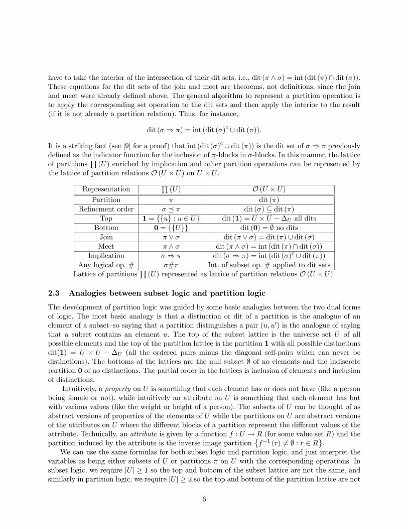
have to take the interior of the intersection of their dit sets, i.e., dit (π ∧ σ) = int (dit (π) ∩ dit (σ)).These equations for the dit sets of the join and meet are theorems, not definitions, since the joinand meet were already defined above. The general algorithm to represent a partition operation isto apply the corresponding set operation to the dit sets and then apply the interior to the result(if it is not already a partition relation). Thus, for instance,

dit (σ ⇒ π) = int (dit (σ)c ∪ dit (π)).

It is a striking fact (see [9] for a proof) that int (dit (σ)c ∪ dit (π)) is the dit set of σ ⇒ π previouslydefined as the indicator function for the inclusion of π-blocks in σ-blocks. In this manner, the latticeof partitions

∏(U) enriched by implication and other partition operations can be represented by

the lattice of partition relations O (U × U) on U × U .

Representation∏

(U) O (U × U)

Partition π dit (π)

Refinement order σ � π dit (σ) ⊆ dit (π)

Top 1 = {{u} : u ∈ U} dit (1) = U × U −∆U all ditsBottom 0 = {{U}} dit (0) = ∅ no ditsJoin π ∨ σ dit (π ∨ σ) = dit (π) ∪ dit (σ)

Meet π ∧ σ dit (π ∧ σ) = int (dit (π) ∩ dit (σ))

Implication σ ⇒ π dit (σ ⇒ π) = int (dit (σ)c ∪ dit (π))

Any logical op. # σ#π Int. of subset op. # applied to dit setsLattice of partitions

∏(U) represented as lattice of partition relations O (U × U).

2.3 Analogies between subset logic and partition logic

The development of partition logic was guided by some basic analogies between the two dual formsof logic. The most basic analogy is that a distinction or dit of a partition is the analogue of anelement of a subset—so saying that a partition distinguishes a pair (u, u′) is the analogue of sayingthat a subset contains an element u. The top of the subset lattice is the universe set U of allpossible elements and the top of the partition lattice is the partition 1 with all possible distinctionsdit(1) = U × U − ∆U (all the ordered pairs minus the diagonal self-pairs which can never bedistinctions). The bottoms of the lattices are the null subset ∅ of no elements and the indiscretepartition 0 of no distinctions. The partial order in the lattices is inclusion of elements and inclusionof distinctions.

Intuitively, a property on U is something that each element has or does not have (like a personbeing female or not), while intuitively an attribute on U is something that each element has butwith various values (like the weight or height of a person). The subsets of U can be thought of asabstract versions of properties of the elements of U while the partitions on U are abstract versionsof the attributes on U where the different blocks of a partition represent the different values of theattribute. Technically, an attribute is given by a function f : U → R (for some value set R) and thepartition induced by the attribute is the inverse image partition

{f−1 (r) 6= ∅ : r ∈ R

}.

We can use the same formulas for both subset logic and partition logic, and just interpret thevariables as being either subsets of U or partitions π on U with the corresponding operations. Insubset logic, we require |U | ≥ 1 so the top and bottom of the subset lattice are not the same, andsimilarly in partition logic, we require |U | ≥ 2 so the top and bottom of the partition lattice are not

6

the same. A formula is a subset tautology if for any universe U (|U | ≥ 1) and for any subsets of Usubstituted for the variables, the result of applying the subset operations is the top of the lattice U ,i.e., the subset formula holds of all elements. A partition tautology is defined analogously. That is,a formula is a partition tautology if for any U (|U | ≥ 2) and for any partitions on U substituted forthe variables, the result of applying the partition operations is the top of the lattice, the discretepartition 1, i.e., the partition formula distinguishes all pairs (u, u′) of distinct elements.

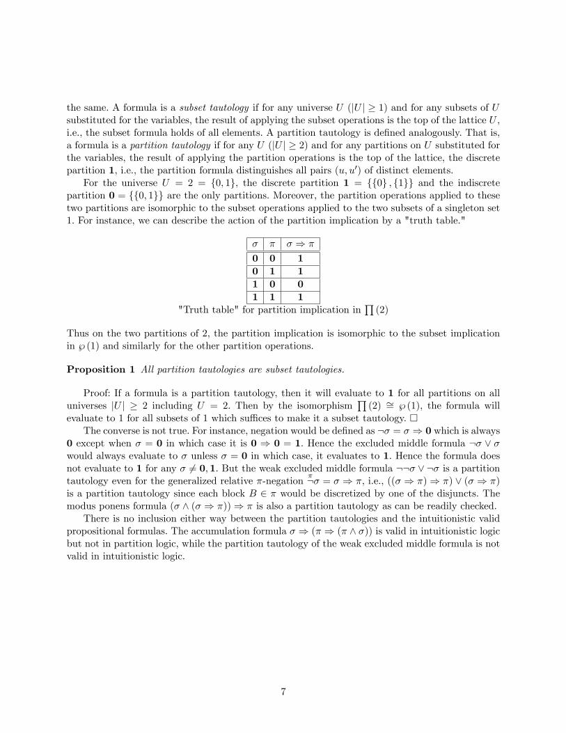
For the universe U = 2 = {0, 1}, the discrete partition 1 = {{0} , {1}} and the indiscretepartition 0 = {{0, 1}} are the only partitions. Moreover, the partition operations applied to thesetwo partitions are isomorphic to the subset operations applied to the two subsets of a singleton set1. For instance, we can describe the action of the partition implication by a "truth table."

σ π σ ⇒ π

0 0 1

0 1 1

1 0 0

1 1 1

"Truth table" for partition implication in∏

(2)

Thus on the two partitions of 2, the partition implication is isomorphic to the subset implicationin ℘ (1) and similarly for the other partition operations.

Proposition 1 All partition tautologies are subset tautologies.

Proof: If a formula is a partition tautology, then it will evaluate to 1 for all partitions on alluniverses |U | ≥ 2 including U = 2. Then by the isomorphism

∏(2) ∼= ℘ (1), the formula will

evaluate to 1 for all subsets of 1 which suffi ces to make it a subset tautology. �The converse is not true. For instance, negation would be defined as ¬σ = σ ⇒ 0 which is always

0 except when σ = 0 in which case it is 0 ⇒ 0 = 1. Hence the excluded middle formula ¬σ ∨ σwould always evaluate to σ unless σ = 0 in which case, it evaluates to 1. Hence the formula doesnot evaluate to 1 for any σ 6= 0,1. But the weak excluded middle formula ¬¬σ ∨ ¬σ is a partitiontautology even for the generalized relative π-negation

π¬σ = σ ⇒ π, i.e., ((σ ⇒ π)⇒ π) ∨ (σ ⇒ π)is a partition tautology since each block B ∈ π would be discretized by one of the disjuncts. Themodus ponens formula (σ ∧ (σ ⇒ π))⇒ π is also a partition tautology as can be readily checked.

There is no inclusion either way between the partition tautologies and the intuitionistic validpropositional formulas. The accumulation formula σ ⇒ (π ⇒ (π ∧ σ)) is valid in intuitionistic logicbut not in partition logic, while the partition tautology of the weak excluded middle formula is notvalid in intuitionistic logic.

7

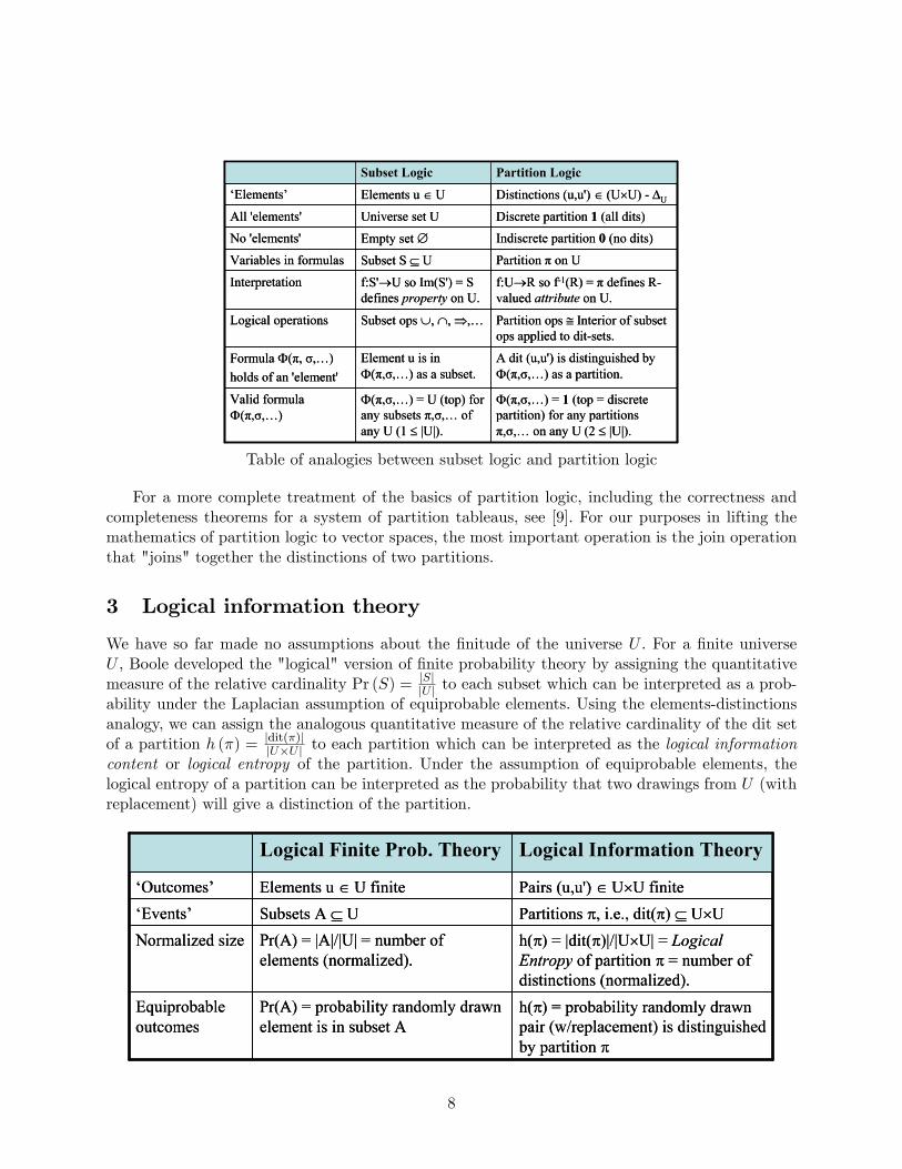
Table of analogies between subset logic and partition logic

For a more complete treatment of the basics of partition logic, including the correctness andcompleteness theorems for a system of partition tableaus, see [9]. For our purposes in lifting themathematics of partition logic to vector spaces, the most important operation is the join operationthat "joins" together the distinctions of two partitions.

3 Logical information theory

We have so far made no assumptions about the finitude of the universe U . For a finite universeU , Boole developed the "logical" version of finite probability theory by assigning the quantitativemeasure of the relative cardinality Pr (S) = |S|

|U | to each subset which can be interpreted as a prob-ability under the Laplacian assumption of equiprobable elements. Using the elements-distinctionsanalogy, we can assign the analogous quantitative measure of the relative cardinality of the dit setof a partition h (π) = |dit(π)|

|U×U | to each partition which can be interpreted as the logical informationcontent or logical entropy of the partition. Under the assumption of equiprobable elements, thelogical entropy of a partition can be interpreted as the probability that two drawings from U (withreplacement) will give a distinction of the partition.

8

Logical probability theory is to subset logicas logical information theory is to partition logic

The probability of drawing an element from a block B ∈ π is pB = |B||U | so the logical entropy of a

partition can be written in terms of these block probabilities since |dit (π)| =∑

B 6=B′∈π |B ×B′| =|U |2 −

∑B∈π |B|

2. Hence:

h (π) = |dit(π)||U×U | =

|U |2−∑B∈π |B|

2

|U |2 = 1−∑

B∈π p2B.

This formula has a long history (see [8]) and is usually called the Gini-Simpson diversity indexin the biological literature [22]. For instance, if we partition animals by species, then it is theprobability in two independent samples that we will find animals of different species.

This version of the logical entropy formula also makes clear the generalization path to definethe logical entropy of any finite probability distribution p = (p1, ..., pn):

h (p) = 1−∑

i p2i .7

C. R. Rao [22] has defined a general notion of quadratic entropy in terms of a distance functiond(u, u′) between the elements of U . In the most general "logical" case, the natural logical distancefunction is:

d (u, u′) = 1− δ (u, u′) =

{1 if u 6= u′

0 if u = u′

and, in that case, the quadratic entropy is just the logical entropy.The Shannon entropy for a partition:

H (π) =∑

B∈π pB log2

(1pB

)can also be interpreted in terms of distinctions. In the special case where π has 2n equal-sized

blocks, then H (π) = 2n 12n log2

(1

1/2n

)= log2 (2n) = n. Think of the 2n blocks as being enumerated

by an n-digit binary number. Then the n questions, "Is the ith digit a 1?" will partition the blocksinto two equal groups and thus will partition U into two equal blocks. Thus each of the n questionsgives a binary partition of U into two equal parts, and the join of those n binary partitions is

the original partition π. Thus the Shannon entropy H (π) = log2

(1pB

)= log2

(1

1/2n

)= n in this

case is the number of equal binary partitions ("bits") necessary to make all the distinctions of π.

The general formula H (π) =∑

B∈π pB log2

(1pB

)can then be seen as the average number of equal

binary partitions or bits necessary to make all the distinctions of π. In contrast, the logical entropyh (π) involves no averaging in its interpretation as the normalized number of distinctions in π.

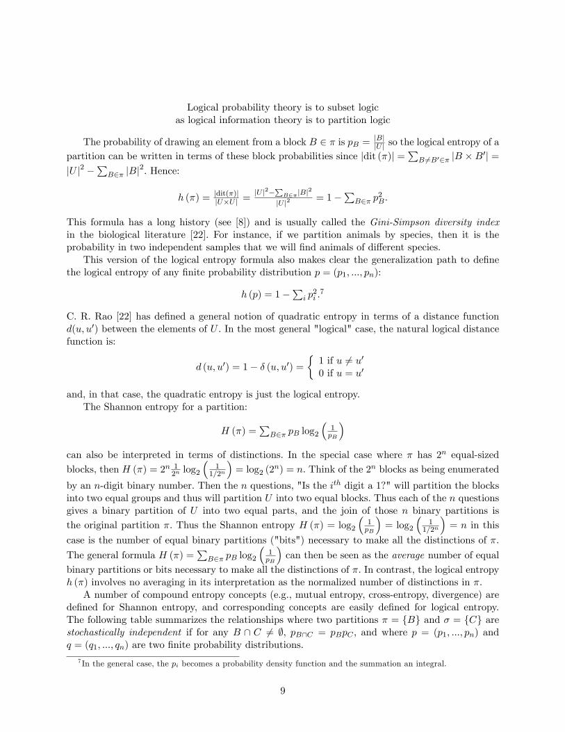
A number of compound entropy concepts (e.g., mutual entropy, cross-entropy, divergence) aredefined for Shannon entropy, and corresponding concepts are easily defined for logical entropy.The following table summarizes the relationships where two partitions π = {B} and σ = {C} arestochastically independent if for any B ∩ C 6= ∅, pB∩C = pBpC , and where p = (p1, ..., pn) andq = (q1, ..., qn) are two finite probability distributions.

7 In the general case, the pi becomes a probability density function and the summation an integral.

9

Corresponding concepts for Shannon entropy and logical entropy

Further details about logical information theory can be found in [8]. For our purposes here,the important thing is the lifting of logical entropy to the context of vector spaces and quantummathematics where for any density matrix ρ, the logical entropy h (ρ) = 1 − tr

[ρ2]allows us to

directly measure and interpret the changes made in a measurement.

4 Partitions and objective indefiniteness

4.1 Representing objective indistinctness

It has already been emphasized how Boolean subset logic captures at the logical level the commonsense vision of reality where an entity definitely has or does not have any property. We can nowdescribe how the dual logic of partitions captures at the logical level a vision of reality with ob-jectively indefinite (or indistinct)8 entities. The key step is to interpret a subset such as a block Bin a partition, not as a subset of the distinct elements u ∈ B, but as a single objectively indistinctelement that, with further distinctions, could become any of the fully distinct elements u ∈ B. Toanticipate the lifted concepts in vector spaces, the fully distinct elements u ∈ U might be called"eigen-elements" and the single indistinct element B is a "superposition" of the eigen-elementsu ∈ B (thinking of the collecting together {u, u′, ...} = B of the elements of B as their "superposi-tion"). With distinctions, the indistinct element B might be refined into one of the singletons {u}for u ∈ B [where {u} is the "superposition" consisting of a single eigen-element so it just denotesthat element u].

Abner Shimony ([25] and [26]), in his description of a superposition state as being objectivelyindefinite, adopted Heisenberg’s [15] language of "potentiality" and "actuality" to describe therelationship of the eigenstates that are superposed to give an objectively indefinite superposition.This terminology could be adapted to the case of the sets. The elements u ∈ B are "potential" inthe objectively indefinite "superposition" B, and, with further distinctions, the indefinite elementB might "actualize" to {u} for one of the "potential" u ∈ B. Starting with B, the other u /∈ B arenot "potentialities" that could be "actualized" with further distinctions.

8The adjectives "indefinite" and "indistinct" will be used interchangeably as synonyms. The word "indefiniteness"is more common in the QM literature, but "indistinctness" has a better noun form as "indistinctions" (with theopposite as "distinctions").

10

This terminology is, however, somewhat misleading since the indefinite element B is perfectlyactual; it is only the multiple eigen-elements u ∈ B that are "potential" until "actualized" bysome further distinctions. In a "measurement," a single actual indefinite element becomes a singleactual definite element. Since the "measurement" goes from actual indefinite to actual definite, thepotential-to-actual language of Heisenberg should only be used with proper care—if at all.

Consider a three-element universe U = {a, b, c} and a partition π = {{a} , {b, c}}. The block{b, c} is objectively indefinite between {b} and {c} so those singletons are its "potentialities" in thesense that a distinction could result in either {b} or {c} being "actualized." However {a} is not a"potentiality" when one is starting with the indefinite element {b, c}.

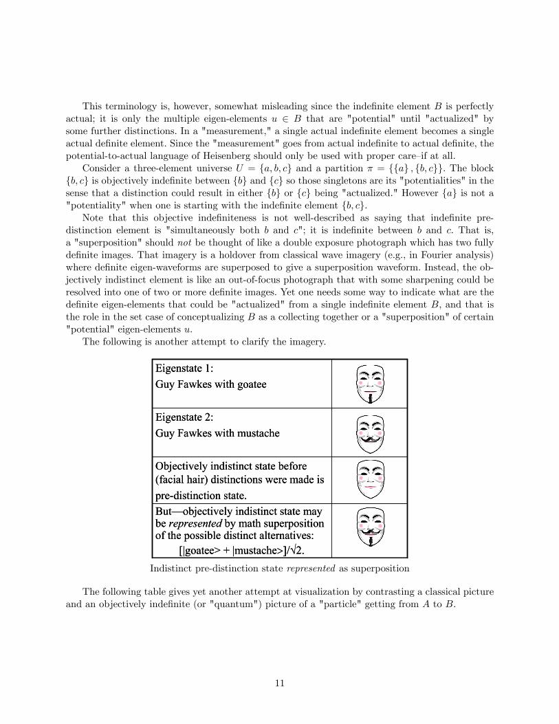
Note that this objective indefiniteness is not well-described as saying that indefinite pre-distinction element is "simultaneously both b and c"; it is indefinite between b and c. That is,a "superposition" should not be thought of like a double exposure photograph which has two fullydefinite images. That imagery is a holdover from classical wave imagery (e.g., in Fourier analysis)where definite eigen-waveforms are superposed to give a superposition waveform. Instead, the ob-jectively indistinct element is like an out-of-focus photograph that with some sharpening could beresolved into one of two or more definite images. Yet one needs some way to indicate what are thedefinite eigen-elements that could be "actualized" from a single indefinite element B, and that isthe role in the set case of conceptualizing B as a collecting together or a "superposition" of certain"potential" eigen-elements u.

The following is another attempt to clarify the imagery.

Indistinct pre-distinction state represented as superposition

The following table gives yet another attempt at visualization by contrasting a classical pictureand an objectively indefinite (or "quantum") picture of a "particle" getting from A to B.

11

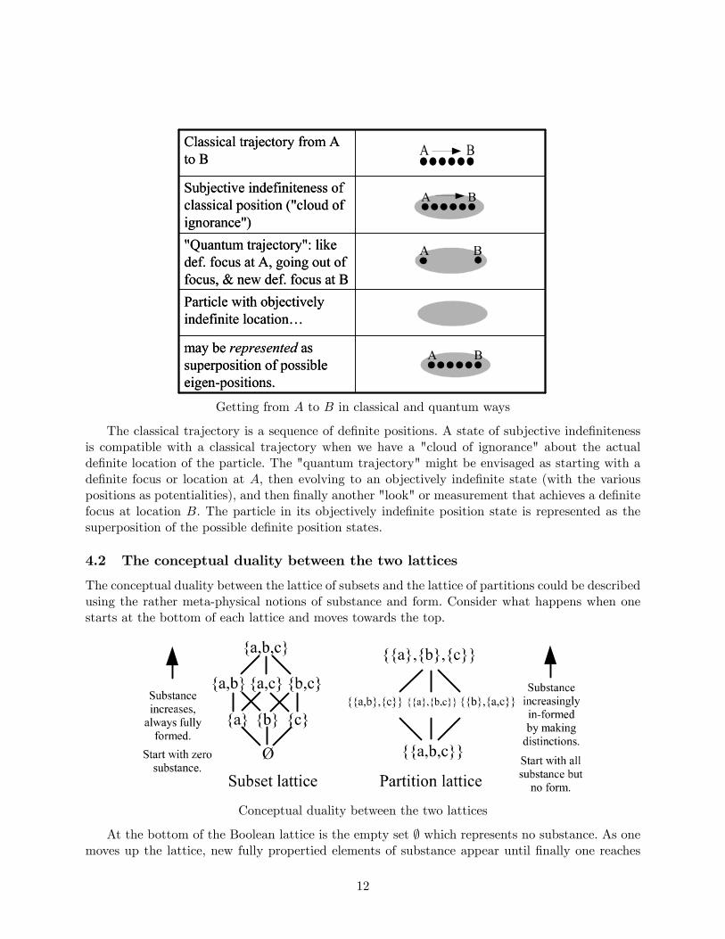
Getting from A to B in classical and quantum ways

The classical trajectory is a sequence of definite positions. A state of subjective indefinitenessis compatible with a classical trajectory when we have a "cloud of ignorance" about the actualdefinite location of the particle. The "quantum trajectory" might be envisaged as starting with adefinite focus or location at A, then evolving to an objectively indefinite state (with the variouspositions as potentialities), and then finally another "look" or measurement that achieves a definitefocus at location B. The particle in its objectively indefinite position state is represented as thesuperposition of the possible definite position states.

4.2 The conceptual duality between the two lattices

The conceptual duality between the lattice of subsets and the lattice of partitions could be describedusing the rather meta-physical notions of substance and form. Consider what happens when onestarts at the bottom of each lattice and moves towards the top.

Conceptual duality between the two lattices

At the bottom of the Boolean lattice is the empty set ∅ which represents no substance. As onemoves up the lattice, new fully propertied elements of substance appear until finally one reaches

12

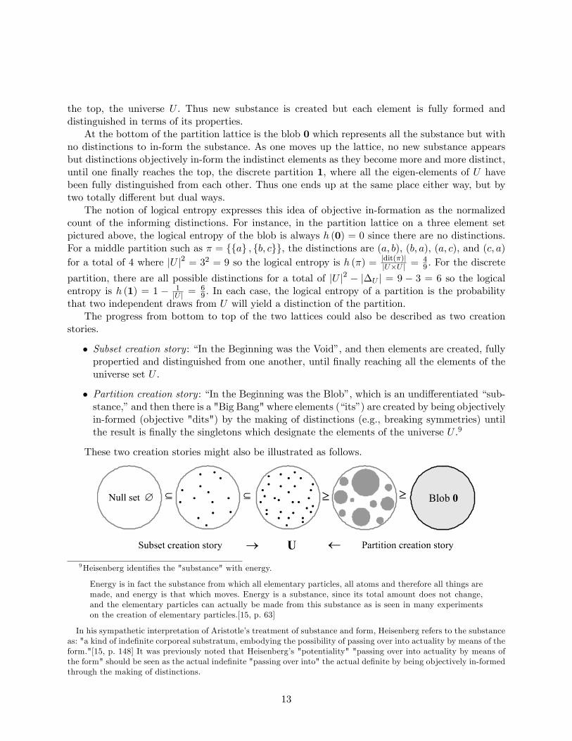
the top, the universe U . Thus new substance is created but each element is fully formed anddistinguished in terms of its properties.

At the bottom of the partition lattice is the blob 0 which represents all the substance but withno distinctions to in-form the substance. As one moves up the lattice, no new substance appearsbut distinctions objectively in-form the indistinct elements as they become more and more distinct,until one finally reaches the top, the discrete partition 1, where all the eigen-elements of U havebeen fully distinguished from each other. Thus one ends up at the same place either way, but bytwo totally different but dual ways.

The notion of logical entropy expresses this idea of objective in-formation as the normalizedcount of the informing distinctions. For instance, in the partition lattice on a three element setpictured above, the logical entropy of the blob is always h (0) = 0 since there are no distinctions.For a middle partition such as π = {{a} , {b, c}}, the distinctions are (a, b), (b, a), (a, c), and (c, a)

for a total of 4 where |U |2 = 32 = 9 so the logical entropy is h (π) = |dit(π)||U×U | = 4

9 . For the discrete

partition, there are all possible distinctions for a total of |U |2 − |∆U | = 9 − 3 = 6 so the logicalentropy is h (1) = 1 − 1

|U | = 69 . In each case, the logical entropy of a partition is the probability

that two independent draws from U will yield a distinction of the partition.The progress from bottom to top of the two lattices could also be described as two creation

stories.

• Subset creation story : “In the Beginning was the Void”, and then elements are created, fullypropertied and distinguished from one another, until finally reaching all the elements of theuniverse set U .

• Partition creation story : “In the Beginning was the Blob”, which is an undifferentiated “sub-stance,”and then there is a "Big Bang" where elements (“its”) are created by being objectivelyin-formed (objective "dits") by the making of distinctions (e.g., breaking symmetries) untilthe result is finally the singletons which designate the elements of the universe U .9

These two creation stories might also be illustrated as follows.

9Heisenberg identifies the "substance" with energy.

Energy is in fact the substance from which all elementary particles, all atoms and therefore all things aremade, and energy is that which moves. Energy is a substance, since its total amount does not change,and the elementary particles can actually be made from this substance as is seen in many experimentson the creation of elementary particles.[15, p. 63]

In his sympathetic interpretation of Aristotle’s treatment of substance and form, Heisenberg refers to the substanceas: "a kind of indefinite corporeal substratum, embodying the possibility of passing over into actuality by means of theform."[15, p. 148] It was previously noted that Heisenberg’s "potentiality" "passing over into actuality by means ofthe form" should be seen as the actual indefinite "passing over into" the actual definite by being objectively in-formedthrough the making of distinctions.

13

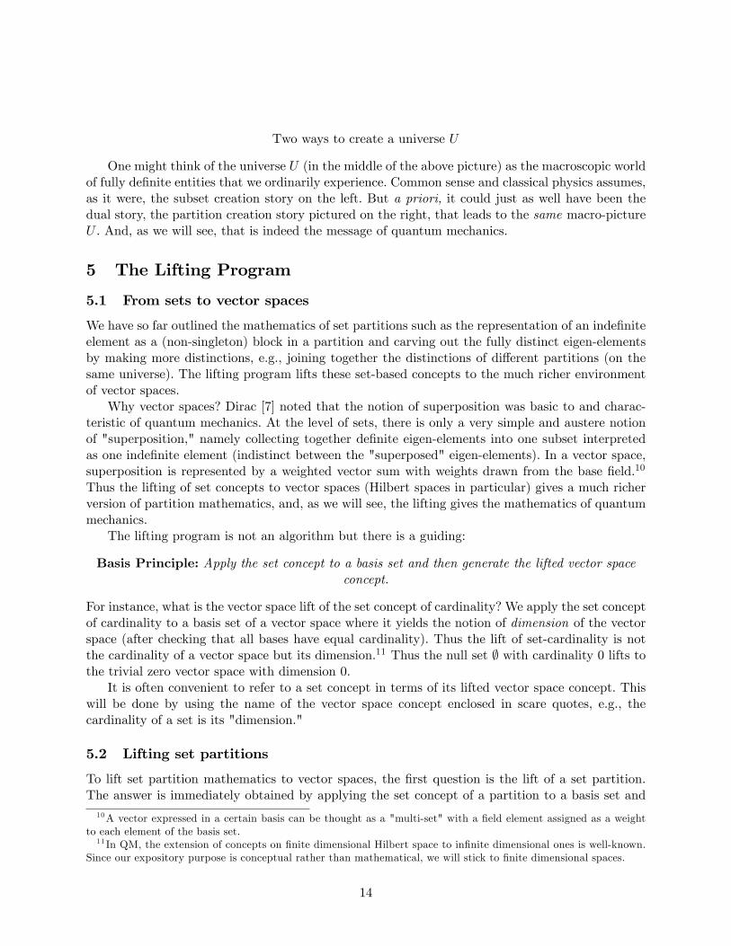
Two ways to create a universe U

One might think of the universe U (in the middle of the above picture) as the macroscopic worldof fully definite entities that we ordinarily experience. Common sense and classical physics assumes,as it were, the subset creation story on the left. But a priori, it could just as well have been thedual story, the partition creation story pictured on the right, that leads to the same macro-pictureU . And, as we will see, that is indeed the message of quantum mechanics.

5 The Lifting Program

5.1 From sets to vector spaces

We have so far outlined the mathematics of set partitions such as the representation of an indefiniteelement as a (non-singleton) block in a partition and carving out the fully distinct eigen-elementsby making more distinctions, e.g., joining together the distinctions of different partitions (on thesame universe). The lifting program lifts these set-based concepts to the much richer environmentof vector spaces.

Why vector spaces? Dirac [7] noted that the notion of superposition was basic to and charac-teristic of quantum mechanics. At the level of sets, there is only a very simple and austere notionof "superposition," namely collecting together definite eigen-elements into one subset interpretedas one indefinite element (indistinct between the "superposed" eigen-elements). In a vector space,superposition is represented by a weighted vector sum with weights drawn from the base field.10

Thus the lifting of set concepts to vector spaces (Hilbert spaces in particular) gives a much richerversion of partition mathematics, and, as we will see, the lifting gives the mathematics of quantummechanics.

The lifting program is not an algorithm but there is a guiding:

Basis Principle: Apply the set concept to a basis set and then generate the lifted vector spaceconcept.

For instance, what is the vector space lift of the set concept of cardinality? We apply the set conceptof cardinality to a basis set of a vector space where it yields the notion of dimension of the vectorspace (after checking that all bases have equal cardinality). Thus the lift of set-cardinality is notthe cardinality of a vector space but its dimension.11 Thus the null set ∅ with cardinality 0 lifts tothe trivial zero vector space with dimension 0.

It is often convenient to refer to a set concept in terms of its lifted vector space concept. Thiswill be done by using the name of the vector space concept enclosed in scare quotes, e.g., thecardinality of a set is its "dimension."

5.2 Lifting set partitions

To lift set partition mathematics to vector spaces, the first question is the lift of a set partition.The answer is immediately obtained by applying the set concept of a partition to a basis set and10A vector expressed in a certain basis can be thought as a "multi-set" with a field element assigned as a weight

to each element of the basis set.11 In QM, the extension of concepts on finite dimensional Hilbert space to infinite dimensional ones is well-known.

Since our expository purpose is conceptual rather than mathematical, we will stick to finite dimensional spaces.

14

then seeing what it generates. Each block B of the set partition of a basis set generates a subspaceWB ⊆ V , and the subspaces together form a direct sum decomposition: V =

∑B ⊕WB. Thus the

proper lifted notion of a partition for a vector space is not a set partition of the space, e.g., definedby a subspace W ⊆ V where v ∼ v′ if v − v′ ∈W , but is a direct sum decomposition of the vectorspace.12 Or put the other way around (i.e., delifted), a set partition is a "direct sum decomposition"of a set.

5.3 Lifting partition joins

The main partition operation that we need to lift to vector spaces is the join operation. Twoset partitions cannot be joined unless they are compatible in the sense of being defined on thesame universe set. This notion of compatibility lifts to vector spaces by defining two vector spacepartitions ω = {Wλ} and ξ = {Xµ} on V as being compatible if there is a basis set for V so thatthe two vector space partitions arise from two set partitions of that common basis set.

If two set partitions π = {B} and σ = {C} are compatible, then their join π ∨ σ is defined asthe set partition whose blocks are the non-empty intersections B ∩C. Similar the lifted concept isthat if two vector space partitions ω = {Wλ} and ξ = {Xµ} are compatible, then their join ω∨ ξ isdefined as the vector space partition whose subspaces are the non-zero intersections Wλ ∩Xµ. Andby the definition of compatibility, we could generate the subspaces of the join ω ∨ ξ by the blocksin the join of the two set partitions of the common basis set.

5.4 Lifting attributes

A set partition might be seen as an abstract rendition of the inverse image partition{f−1 (r)

}defined by some concrete attribute f : U → R on U (where we take the value set as the realssince that is also the relevant value set for QM). What is the lift of an attribute? At first glance,the basis principle would seem to imply: define a set attribute on a basis set (with values in thebase field) and then linearly generate a functional from the vector space to the base field. But afunctional does not define a vector space partition; it only defines the set partition of the vectorspace determined by the kernel of the functional. Hence we need to try a more careful applicationof the basis principle.

It is helpful to first give a suggestive reformulation of a set attribute f : U → R. If f is constanton a subset S ⊆ U with a value r, then we might symbolize this as:

f � S = rS

and suggestively call S an "eigenvector" and r an "eigenvalue." For any "eigenvalue" r, definef−1 (r) = "eigenspace of r" as the union of all the "eigenvectors" with that "eigenvalue." Since the"eigenspaces" span the set U , the attribute f : U → R can be represented by:

f =∑

r rχf−1(r)"Spectral decomposition" of set attribute f : U → R

12The usual quantum logic approach to define a ‘propositional’logic for QM focused on the question of whether ornot a vector was in a subspace, which in turn lead to a misplaced focus on the set equivalence relations defined bythe subspaces, equivalence relations that have a special property of being commuting [14]. If "quantum logic" is tobe the logic that is to QM as Boolean subset logic is to classical mechanics, then that is partition logic.

15

[where χf−1(r) is the characteristic function for the "eigenspace" f−1 (r)]. Thus a set attribute

determines a set partition and has a constant value on the blocks of the set partition, so by thebasis principle, that lifts to a vector space concept that determines a vector space partition andhas a constant value on the blocks of a vector space partition.

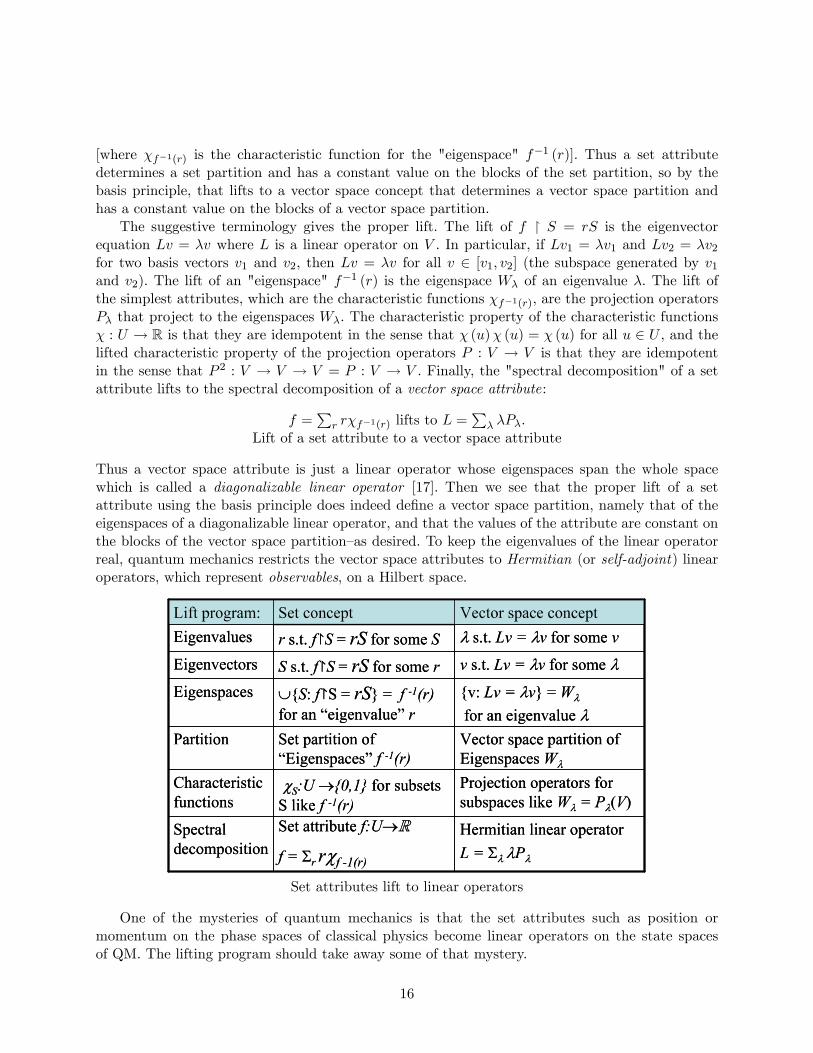
The suggestive terminology gives the proper lift. The lift of f � S = rS is the eigenvectorequation Lv = λv where L is a linear operator on V . In particular, if Lv1 = λv1 and Lv2 = λv2for two basis vectors v1 and v2, then Lv = λv for all v ∈ [v1, v2] (the subspace generated by v1and v2). The lift of an "eigenspace" f−1 (r) is the eigenspace Wλ of an eigenvalue λ. The lift ofthe simplest attributes, which are the characteristic functions χf−1(r), are the projection operatorsPλ that project to the eigenspaces Wλ. The characteristic property of the characteristic functionsχ : U → R is that they are idempotent in the sense that χ (u)χ (u) = χ (u) for all u ∈ U , and thelifted characteristic property of the projection operators P : V → V is that they are idempotentin the sense that P 2 : V → V → V = P : V → V . Finally, the "spectral decomposition" of a setattribute lifts to the spectral decomposition of a vector space attribute:

f =∑

r rχf−1(r) lifts to L =∑

λ λPλ.Lift of a set attribute to a vector space attribute

Thus a vector space attribute is just a linear operator whose eigenspaces span the whole spacewhich is called a diagonalizable linear operator [17]. Then we see that the proper lift of a setattribute using the basis principle does indeed define a vector space partition, namely that of theeigenspaces of a diagonalizable linear operator, and that the values of the attribute are constant onthe blocks of the vector space partition—as desired. To keep the eigenvalues of the linear operatorreal, quantum mechanics restricts the vector space attributes to Hermitian (or self-adjoint) linearoperators, which represent observables, on a Hilbert space.

Set attributes lift to linear operators

One of the mysteries of quantum mechanics is that the set attributes such as position ormomentum on the phase spaces of classical physics become linear operators on the state spacesof QM. The lifting program should take away some of that mystery.

16

5.5 Lifting compatible attributes

Since two set attributes f : U → R and g : U ′ → R define two inverse image partitions{f−1 (r)

}and

{g−1 (s)

}on their domains, we need to extend the concept of compatible partitions to the

attributes that define the partitions. That is, two attributes f : U → R and g : U ′ → R arecompatible if they have the same domain U = U ′.13 We have previously lifted the notion of com-patible set partitions to compatible vector space partitions. Since real-valued set attributes lift toHermitian linear operators, the notion of compatible set attributes just defined would lift to twolinear operators being compatible if their eigenspace partitions are compatible. It is a standard factof the QM literature (e.g., [18, pp. 102-3] or [17, p. 177]) that two (Hermitian) linear operatorsL,M : V → V are compatible if and only if they commute, LM = ML. Hence the commutativityof linear operators is the lift of the compatibility (i.e., defined on the same set) of set attributes.

Given two compatible set attributes f : U → R and g : U → R, the join of their "eigenspace"partitions has as blocks the non-empty intersections f−1 (r) ∩ g−1 (s). Each block in the join ofthe "eigenspace" partitions could be characterized by the ordered pair of "eigenvalues" (r, s). An"eigenvector" S ⊆ f−1 (r) and S ⊆ g−1 (s) would be a "simultaneous eigenvector": S ⊆ f−1 (r) ∩g−1 (s).

In the lifted case, two commuting Hermitian linear operator L andM have compatible eigenspacepartitions WL = {Wλ} (for the eigenvalues λ of L) and WM = {Wµ} (for the eigenvalues µ of M).The blocks in the join WL ∨ WM of the two compatible eigenspace partitions are the non-zerosubspaces {Wλ ∩Wµ} which can be characterized by the ordered pairs of eigenvalues (λ, µ). Thenonzero vectors v ∈Wλ ∩Wµ are simultaneous eigenvectors for the two commuting operators, andthere is a basis for the space consisting of simultaneous eigenvectors.14

A set of compatible set attributes is said to be complete if the join of their partitions is discrete,i.e., the blocks have cardinality 1. Each element of U is then characterized by the ordered n-tuple(r, ..., s) of attribute values.

In the lifted case, a set of commuting linear operators is said to be complete if the join oftheir eigenspace partitions is nondegenerate, i.e., the blocks have dimension 1. The eigenvectorsthat generate those one-dimensional blocks of the join are characterized by the ordered n-tuples(λ, ..., µ) of eigenvalues so the eigenvectors are usually denoted as the eigenkets |λ, ..., µ〉 in theDirac notation. These Complete Sets of Commuting Operators are Dirac’s CSCOs [7].

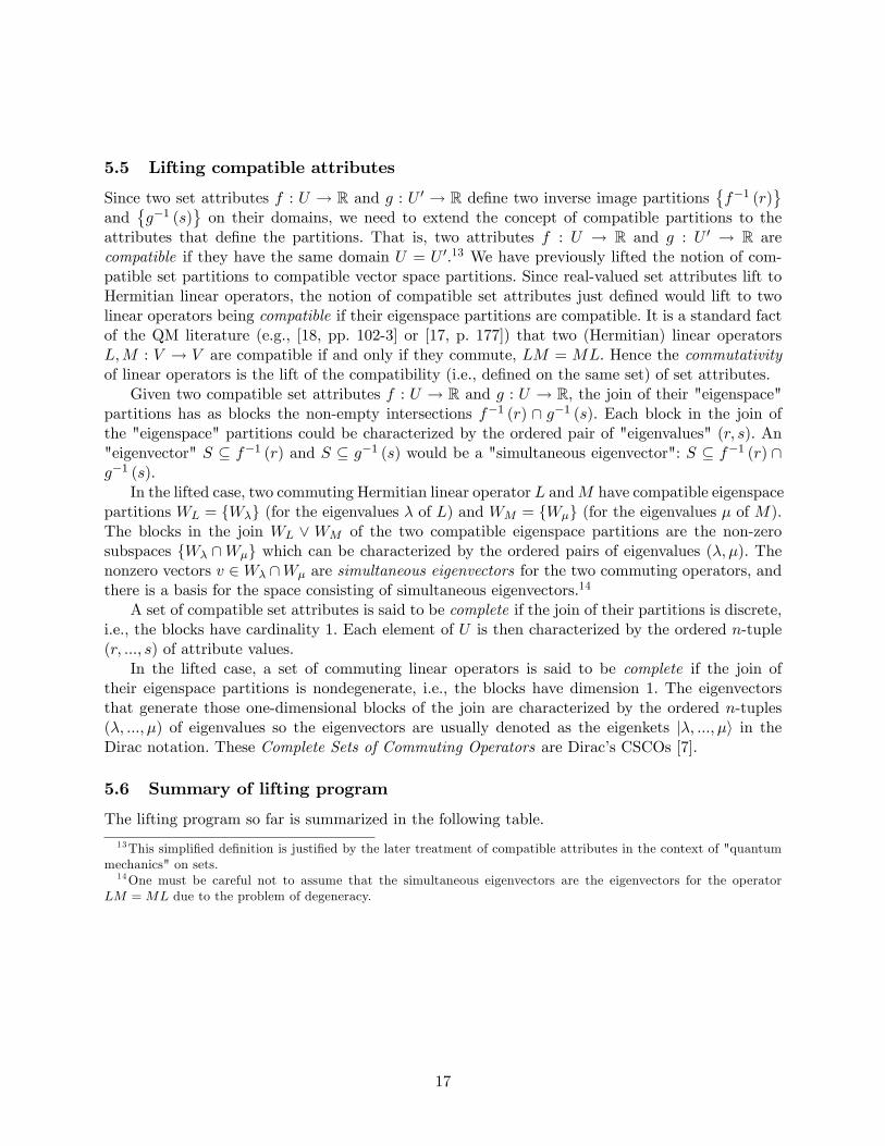
5.6 Summary of lifting program

The lifting program so far is summarized in the following table.

13This simplified definition is justified by the later treatment of compatible attributes in the context of "quantummechanics" on sets.14One must be careful not to assume that the simultaneous eigenvectors are the eigenvectors for the operator

LM = ML due to the problem of degeneracy.

17

Summary of Lifts

5.7 Some subtleties of the lifting program

The relation between set concepts and the lifted vector space concepts is not a one-to-one map-ping.15 For instance, the same subset S = f−1 (r) appears both as an "eigenvector" S such thatf � S = rS and as an "eigenspace"—which are two very different vector space concepts. The two-dimensional space [a, b] generated by vectors a and b is quite different from the vector a + b, butat the austere level of sets, they are both {a, b}. Thus the same set concept of a subset {a, b}(depending on whether it is viewed as {a, b} = f−1 (r) or as f � {a, b} = r {a, b}) lifts to quitedifferent vector space concepts: the subspace [a, b] or the vector a + b. This is one of the reasonsthat the lifting program cannot be reduced to a simple mapping.

Moreover, the same vector space concept, viewed from different angles, may "delift" to quitedifferent set concepts. Consider the vector space concept of a projection operator P : V → V thatprojects to the subspace P (V ) = W . As a linear operator with the eigenvalues 0 and 1, a projectionoperator is the lift of a characteristic function χS : U → R as an attribute. The projection operatorassigns the eigenvalues 1 and 0 to the two blocks P (V ) and ker (P ) of its eigenspace partition, justas the attribute χS assigns the two values to the two blocks χS (1) and χS (0) of its set partition.But a projection operator also serves to project an arbitrary vector v ∈ V to the part of v, namelyP (v), that is in the range-space W . Since the delift of vectors v ∈ V are subsets S ⊆ U (viewed assingle indefinite elements), the delift of the projecting operation would be a mapping from arbitrarysubsets to the part of each subset that is in the "range eigenspace" χ−1S (1). That "projection" isthe idempotent mapping:

χ−1S (1) ∩ () : ℘ (U)→ ℘ (U).

Thus the same vector space concept of a projection operator delifts to two quite different setconcepts: the set attribute χS : U → R and the subset operator χ−1S (1) ∩ () : ℘ (U)→ ℘ (U).

15Perhaps the lifting program is akin to a type of mathematical "pornography"—it is hard to define exactly but youknow it when you see it.

18

The subset operator treatment of a projection allows another type of "spectral decomposition"associated with an attribute f : U → R. The previous statement for S ⊆ f−1 (r) that f � S = rScan now be written r

[f−1 (r) ∩ S

]= rS so that the action of f on subsets can be symbolically

represented as:

f � () =∑

r r[f−1 (r) ∩ ()

]that identifies the "eigenvectors" and "eigenvalues" in the set case and thus could be taken as theset operator analogue of L =

∑λ λPλ.

6 The Delifting Program: "Quantum mechanics" on sets

6.1 Probabilities in "quantum mechanics" on sets

The lifting program establishes a relationship between concepts and operations for sets and thosefor vector spaces. We have so far started with set concepts, like the concept of a set partition, andthen developed the corresponding concept for vector spaces (direct sum decomposition). Howeverthe relation between set and vector space concepts can also be established by going the other way,by delifting quantum mechanical concepts from vector spaces to sets. By delifting QM conceptsto sets, we can develop a toy model called "quantum mechanics" on sets—which shows the logicalstructure of QM in a pedagogically simple and understandable context.

The connection between sets and the complex vector spaces of QM can be facilitated by consid-ering an intermediate stage. A power set ℘ (U) can be considered as a vector space over Z2 = {0, 1}with the symmetric difference of subsets, i.e., S∆T = S ∪ T − S ∩ T for S, T ⊆ U , as the vectoraddition operation. Thus set concepts can be first translated into sets-as-vectors concepts for vectorspaces over Z2 and then lifted to vector spaces over C (or vice-versa for delifting). One of the keypieces of machinery in QM, namely the inner product, does not exist in vector spaces over finitefields but a norm can be defined to play a similar role in the probability algorithm.

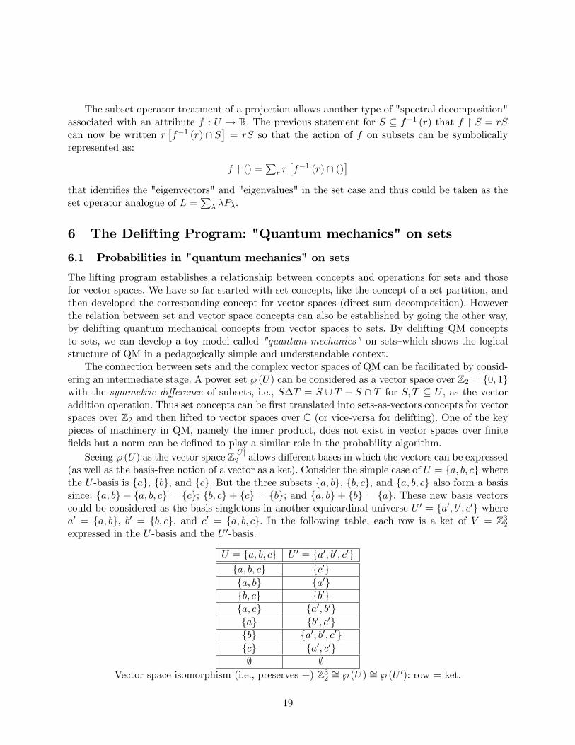
Seeing ℘ (U) as the vector space Z|U |2 allows different bases in which the vectors can be expressed(as well as the basis-free notion of a vector as a ket). Consider the simple case of U = {a, b, c} wherethe U -basis is {a}, {b}, and {c}. But the three subsets {a, b}, {b, c}, and {a, b, c} also form a basissince: {a, b} + {a, b, c} = {c}; {b, c} + {c} = {b}; and {a, b} + {b} = {a}. These new basis vectorscould be considered as the basis-singletons in another equicardinal universe U ′ = {a′, b′, c′} wherea′ = {a, b}, b′ = {b, c}, and c′ = {a, b, c}. In the following table, each row is a ket of V = Z32expressed in the U -basis and the U ′-basis.

U = {a, b, c} U ′ = {a′, b′, c′}{a, b, c} {c′}{a, b} {a′}{b, c} {b′}{a, c} {a′, b′}{a} {b′, c′}{b} {a′, b′, c′}{c} {a′, c′}∅ ∅

Vector space isomorphism (i.e., preserves +) Z32 ∼= ℘ (U) ∼= ℘ (U ′): row = ket.

19

In a Hilbert space, the inner product is used to define the norm ‖v‖ =√〈v|v〉, and the

probability algorithm can be formulated using this norm. In a vector space over Z2, the Diracnotation can still be used to define a real-valued norm even though there is no inner product.The kets |S〉 for S ∈ ℘ (U) are basis-free but the corresponding bras are basis-dependent. Foru ∈ U , the bra 〈{u}|U : ℘ (U) → R is defined: 〈{u} |US〉 = 1 if u ∈ S and 0 otherwise so that〈{} |US〉 = χS : U → {0, 1}. Assuming a finite U , the bra can also be defined in a more generalbasis-dependent form:

〈T |US〉 = |T ∩ S| for T, S ⊆ U .

Note that for u, u′ ∈ U , 〈{u′} |U {u}〉 = δu′u taking the distinct elements of U as being paired withthe vectors in an orthonormal basis in the lift-delift relationship. In fact, this delifting of the Diracbracket is easily motivated by considering an orthonormal basis set {|u〉} in a finite dimensionalHilbert space. Given two subsets T, S ⊆ {|u〉}, consider the unnormalized vector ψT =

∑|u〉∈T |u〉

and similarly for ψS . Then their inner product in the Hilbert space is 〈ψT |ψS〉 = |T ∩ S|, which"delifts" (running the basis principle in reverse) to 〈T |US〉 = |T ∩ S| for subsets T, S ⊆ U .

Then the U -norm ‖S‖U : ℘ (U)→ R is defined, as usual, as the square root of the bracket:

‖S‖U =√〈S|US〉 =

√|S|

for S ∈ ℘ (U) which is the delift of the basis-free norm ‖ψ‖ =√〈ψ|ψ〉 (since the inner product

does not depend on the basis). Note that a ket has to be expressed in the U -basis to apply thebasis-dependent definition so in the above example, ‖{a′}‖U =

√2 since {a′} = {a, b} in the U -basis.

For a specific basis {|vi〉} and for any nonzero vector v in a finite dimensional vector space, ‖v‖ =√∑i 〈vi|v〉 〈vi|v〉

∗ whose delifted version would be: ‖S‖U =√∑

u∈U 〈{u} |US〉2. Thus squaring

both sides, we also have:∑i〈vi|v〉〈vi|v〉∗

‖v‖2 = 1 and∑

u〈{u}|US〉2

‖S‖2U=∑

u|{u}∩S||S| = 1

where 〈vi|v〉〈vi|v〉∗

‖v‖2 is a ‘mysterious’quantum probability while |{u}∩S||S| is the unmysterious probability

Pr ({u} |S) of getting u when sampling S (equiprobable elements of U). We previously saw that asubset S ⊆ U as a block in a partition could be interpreted as a single indefinite element rather thana subset of definite elements. In like manner, we can interpret a subset of outcomes (an event) in afinite probability space as a single indefinite outcome where the conditional probability Pr ({u} |S)is the objective probability of a "U -measurement" of S yielding the definite outcome {u}.

An observable, i.e., a Hermitian operator, on a Hilbert space determines its home basis setof orthonormal eigenvectors. In a similar manner, an attribute f : U → R defined on U has theU -basis as its "home basis set." Then given a Hermitian operator L =

∑λ λPλ and a U -attribute

f : U → R, we have:

‖v‖ =√∑

λ ‖Pλ (v)‖ and ‖S‖U =√∑

r ‖f−1 (r) ∩ S‖2U

where f−1 (r) ∩ S is the "projection operator" f−1 (r) ∩ () applied to S, the delift of applying theprojection operator Pλ to v.16 This can also be written as:16Since ℘ (U) is now interpreted as a vector space, it should be noted that the projection operator S ∩ () : ℘ (U) →

℘ (U) is linear, i.e., (S ∩ S1) ∆(S ∩ S2) = S ∩ (S1∆S2). Indeed, this is the distributive law when ℘ (U) is interpretedas a Boolean ring.

20

∑λ‖Pλ(v)‖2

‖v‖2 = 1 and∑

r‖f−1(r)∩S‖2

U

‖S‖2U=∑

r|f−1(r)∩S||S| = 1

where ‖Pλ(v)‖2

‖v‖2 is the quantum probability of getting λ in an L-measurement of v while |f−1(r)∩S||S| has

the rather unmysterious interpretation of the probability Pr (r|S) of the random variable f : U → Rhaving the value r when sampling S ⊆ U . Under the set version of the objective indefinitenessinterpretation, i.e., "quantum mechanics" on sets, the indefinite element S is being "measured"

using the "observable" f and the probability Pr (r|S) of getting the "eigenvalue" r is |f−1(r)∩S||S|

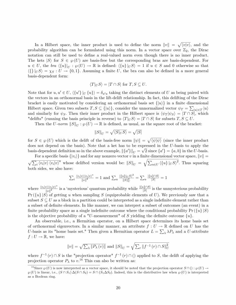
with the "projected resultant state" as f−1 (r) ∩ S.These delifts are summarized in the following table for a finite U and a finite dimensional

Hilbert space V .

Set Case Vector space case

Projection B ∩ () : ℘ (U)→ ℘ (U) Projection P : V → V

f � () =∑

r r(f−1 (r) ∩ ()

)Herm. L =

∑λ λPλ

∆B∈πB ∩ () = I : ℘ (U)→ ℘ (U)∑

λ Pλ = I

〈S|UT 〉 = |S ∩ T | where S, T ⊆ U 〈ψ|ϕ〉 = "overlap" of ψ and ϕ‖S‖U =

√〈S|US〉 =

√|S| where S ⊆ U ‖ψ‖ =

√〈ψ|ψ〉

‖S‖U =√∑

u∈U ‖{u} ∩ S‖2U ‖ψ‖ =

√∑i 〈vi|ψ〉 〈vi|ψ〉

∗

S 6= ∅,∑

u∈U‖{u}∩S‖2U‖S‖2U

=∑

u∈S1|S| = 1 |ψ〉 6= 0,

∑i〈vi|ψ〉〈vi|ψ〉∗

‖ψ‖2 = 1

‖S‖U =√∑

r ‖f−1 (r) ∩ S‖2U ‖ψ‖ =√∑

λ ‖Pλ (ψ)‖2

S 6= ∅,∑

r‖f−1(r)∩S‖2

U

‖S‖2U=∑

r|f−1(r)∩S||S| = 1 |ψ〉 6= 0,

∑λ‖Pλ(ψ)‖2

‖ψ‖2 = 1

Given S, prob. of r is‖f−1(r)∩S‖2

U

‖S‖2U=|f−1(r)∩S||S| Given ψ, prob. of λ is ‖Pλ(ψ)‖

2

‖ψ‖2

Demystifying quantum probabilities using "quantum mechanics" on sets

6.2 Measurement in "quantum mechanics" on sets

Certainly the notion of measurement is one of the most opaque notions of QM so let’s considera set version of (projective) measurement starting at some block (the "state") in a partition in apartition lattice. In the simple example illustrated below we start at the one block or "state" ofthe indiscrete partition or blob which is the completely indistinct element {a, b, c}. A measurementalways uses some attribute that defines an inverse-image partition on U = {a, b, c}. In the case athand, there are "essentially" four possible attributes that could be used to "measure" the indefiniteelement {a, b, c} (since there are four partitions that refine the blob).

For an example of a "nondegenerate measurement," consider any attribute f : U → R which hasthe discrete partition as its inverse image, such as the ordinal number of a letter in the alphabet:f (a) = 1, f (b) = 2, and f (c) = 3. This attribute or "observable" has three "eigenvectors":f � {a} = 1 {a}, f � {b} = 2 {b}, and f � {c} = 3 {c} with the corresponding "eigenvalues." The"eigenspaces" in the inverse image are also {a}, {b}, and {c}, the blocks in the discrete partition ofU all of which have "dimension" (i.e., cardinality) one. Starting in the "state" S = {a, b, c}, a U -measurement with this observable would yield the "eigenvalue" r with the probability of Pr (r|S) =

21

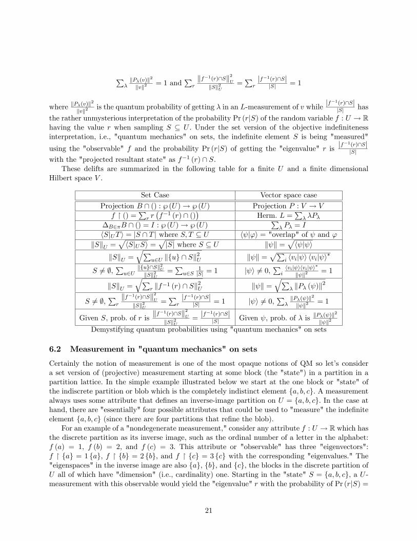
|f−1(r)∩S||S| = 1

3 . A "projective measurement" makes distinctions in the measured "state" that aresuffi cient to induce the "quantum jump" or "projection" to the "eigenvector" associated with theobserved "eigenvalue." If the observed "eigenvalue" was 3, then the "state" {a, b, c} "projects" tof−1 (3) ∩ {a, b, c} = {c} ∩ {a, b, c} = {c} as pictured below.

"Nondegenerate measurement"

It might be emphasized that this is an objective state reduction (or "collapse of the wavepacket") from the single indefinite element {a, b, c} to the single definite element {c}, not a subjec-tive removal of ignorance as if the "state" had all along been {c}. For instance, Pascual Jordan in1934 argued that:

the electron is forced to a decision. We compel it to assume a definite position; previously,in general, it was neither here nor there; it had not yet made its decision for a definiteposition... . ... [W]e ourselves produce the results of the measurement. (quoted in [19,p. 161])

For an example of a "degenerate measurement," we choose an attribute with a non-discreteinverse-image partition such as {{a} , {b, c}}, which could, for instance, just be the characteristicfunction χ{b,c} with the two "eigenspaces" {a} and {b, c} and the two "eigenvalues" 0 and 1 respec-tively. Since one of the two "eigenspaces" is not a singleton of an eigen-element, the "eigenvalue"of 1 is a set version of a "degenerate eigenvalue." This attribute χ{b,c} has four "eigenvectors":χ{b,c} � {b, c} = 1 {b, c}, χ{b,c} � {b} = 1 {b}, χ{b,c} � {c} = 1 {c}, and χ{b,c} � {a} = 0 {a}.

The "measuring apparatus" makes distinctions that further distinguishes the indefinite elementS = {a, b, c} but the measurement returns one of "eigenvalues" with certain probabilities:

Pr(0|S) = |{a}∩{a,b,c}||{a,b,c}| = 1

3 and Pr (1|S) = |{b,c}∩{a,b,c}||{a,b,c}| = 2

3 .

Suppose it returns the "eigenvalue" 1. Then the indefinite element {a, b, c} "jumps" to the"projection" χ−1{b,c} (1) ∩ {a, b, c} = {b, c} of the "state" {a, b, c} to that "eigenspace" [5, p. 221].

Since this is a "degenerate" result (i.e., the "eigenspace" of 1 does not have "dimension" one),another measurement is needed to make more distinctions. Measurements by attributes that giveeither of the other two middle partitions, {{a, b} , {c}} or {{b} , {a, c}}, suffi ce to distinguish {b, c}into {b} or {c}, so either attribute together with the attribute χ{b,c} would form a complete set ofcompatible attributes (i.e., the set version of a CSCO). The join of the two attributes’partitionsgives the discrete partition. Taking the other attribute as χ{a,b}, the join of the two attributes’"eigenspace" partitions is discrete:

22

{{a} , {b, c}} ∨ {{a, b} , {c}} = {{a} , {b} , {c}} = 1.

Hence all the singletons can be characterized by the ordered pairs of the "eigenvalues" of these twoattributes: {a} = |0, 1〉, {b} = |1, 1〉, and {c} = |1, 0〉 (using Dirac’s kets to give the ordered pairs).

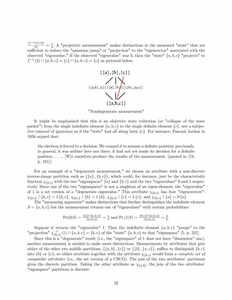
The second "projective measurement" of the indefinite "superposition" element {b, c} using theattribute χ{a,b} with the "eigenspace" partition {{a, b} , {c}} would induce a jump to either {b} or{c} with the probabilities:

Pr (1| {b, c}) = |{a,b}∩{b,c}||{b,c}| = 1

2 and Pr (0| {b, c}) = |{c}∩{b,c}||{b,c}| = 1

2 .

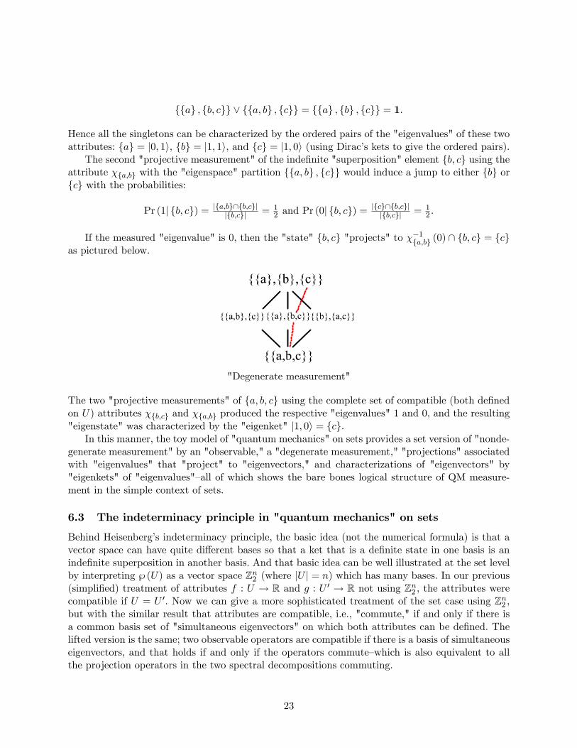
If the measured "eigenvalue" is 0, then the "state" {b, c} "projects" to χ−1{a,b} (0) ∩ {b, c} = {c}as pictured below.

"Degenerate measurement"

The two "projective measurements" of {a, b, c} using the complete set of compatible (both definedon U) attributes χ{b,c} and χ{a,b} produced the respective "eigenvalues" 1 and 0, and the resulting"eigenstate" was characterized by the "eigenket" |1, 0〉 = {c}.

In this manner, the toy model of "quantum mechanics" on sets provides a set version of "nonde-generate measurement" by an "observable," a "degenerate measurement," "projections" associatedwith "eigenvalues" that "project" to "eigenvectors," and characterizations of "eigenvectors" by"eigenkets" of "eigenvalues"—all of which shows the bare bones logical structure of QM measure-ment in the simple context of sets.

6.3 The indeterminacy principle in "quantum mechanics" on sets

Behind Heisenberg’s indeterminacy principle, the basic idea (not the numerical formula) is that avector space can have quite different bases so that a ket that is a definite state in one basis is anindefinite superposition in another basis. And that basic idea can be well illustrated at the set levelby interpreting ℘ (U) as a vector space Zn2 (where |U | = n) which has many bases. In our previous(simplified) treatment of attributes f : U → R and g : U ′ → R not using Zn2 , the attributes werecompatible if U = U ′. Now we can give a more sophisticated treatment of the set case using Zn2 ,but with the similar result that attributes are compatible, i.e., "commute," if and only if there isa common basis set of "simultaneous eigenvectors" on which both attributes can be defined. Thelifted version is the same; two observable operators are compatible if there is a basis of simultaneouseigenvectors, and that holds if and only if the operators commute—which is also equivalent to allthe projection operators in the two spectral decompositions commuting.

23

We are given two basis sets {{a} , {b} , ... | a, b, ... ∈ U} and {{a′} , {b′} , ... | a′, b′, ... ∈ U ′} forZn2 such as in the previous example where n = 3 and the U ′-basis was the three kets {a′} = {a, b},{b′} = {b, c}, and {c′} = {a, b, c}. Then we have two real-valued set attributes defined on thedifferent bases, f : U → R and g : U ′ → R, and we want to investigate their compatibility.

The set attributes define set partitions{f−1 (r)

}and

{g−1 (s)

}respectively on U and U ′.

These set partitions on the basis sets define, as usual, vector space partitions{℘(f−1 (r)

)}and{

℘(g−1 (s)

)}on Zn2 . But those vector space partitions cannot in general be obtained as the

eigenspace partitions of Hermitian operators on Zn2 since the only available eigenvalues are 0 and1. But any set attribute that is the characteristic function χS : U → {0, 1} ⊆ R of a subset S ⊆ Ucan represented by an operator, indeed a projection operator, whose action on ℘ (U) ∼= Zn2 is givenby the "projection operator" S ∩ () : ℘ (U) → ℘ (U), and similarly for U ′. The properties of thereal-valued attributes f and g can then stated in terms of these projection operators for subsetsS = f−1 (r) ⊆ U and S′ = g−1 (s) ⊆ U ′.

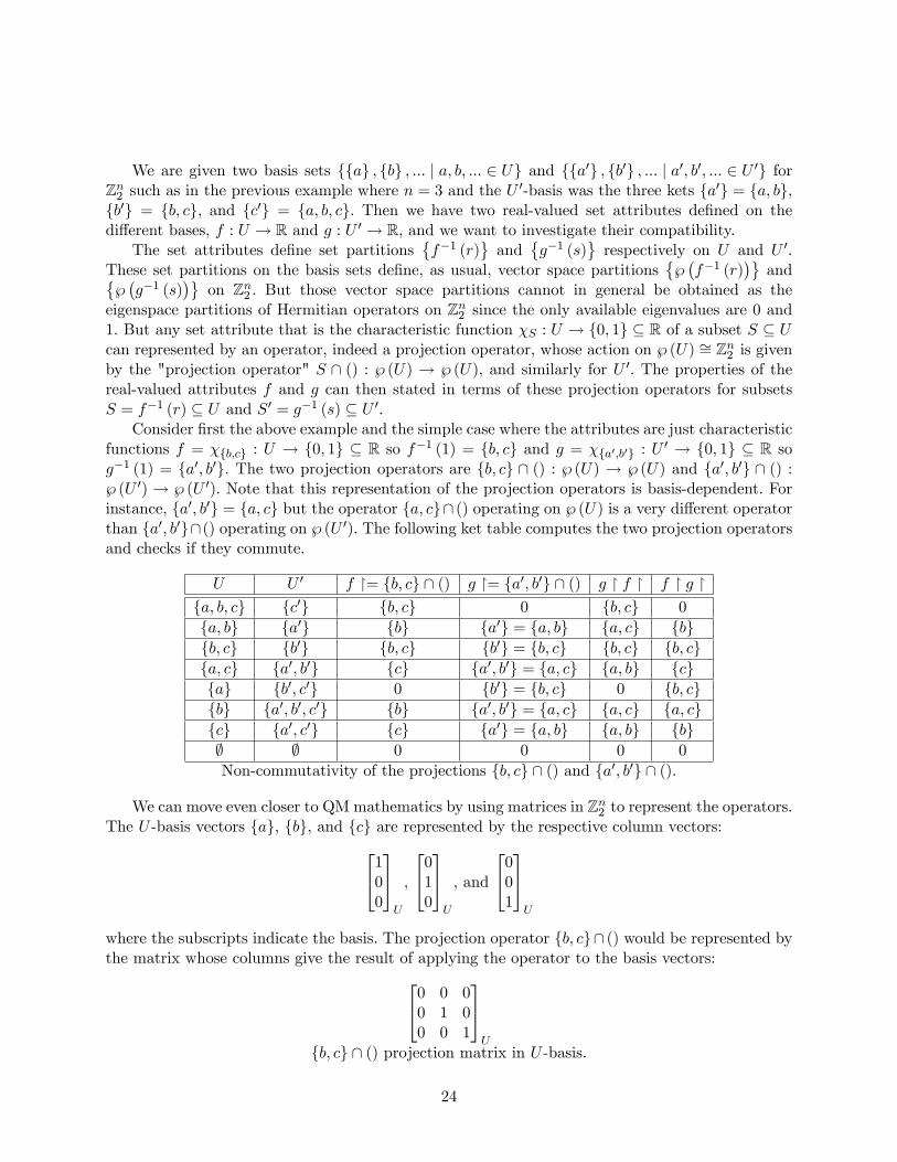
Consider first the above example and the simple case where the attributes are just characteristicfunctions f = χ{b,c} : U → {0, 1} ⊆ R so f−1 (1) = {b, c} and g = χ{a′,b′} : U ′ → {0, 1} ⊆ R sog−1 (1) = {a′, b′}. The two projection operators are {b, c} ∩ () : ℘ (U) → ℘ (U) and {a′, b′} ∩ () :℘ (U ′) → ℘ (U ′). Note that this representation of the projection operators is basis-dependent. Forinstance, {a′, b′} = {a, c} but the operator {a, c}∩ () operating on ℘ (U) is a very different operatorthan {a′, b′}∩() operating on ℘ (U ′). The following ket table computes the two projection operatorsand checks if they commute.

U U ′ f �= {b, c} ∩ () g �= {a′, b′} ∩ () g � f � f � g �{a, b, c} {c′} {b, c} 0 {b, c} 0

{a, b} {a′} {b} {a′} = {a, b} {a, c} {b}{b, c} {b′} {b, c} {b′} = {b, c} {b, c} {b, c}{a, c} {a′, b′} {c} {a′, b′} = {a, c} {a, b} {c}{a} {b′, c′} 0 {b′} = {b, c} 0 {b, c}{b} {a′, b′, c′} {b} {a′, b′} = {a, c} {a, c} {a, c}{c} {a′, c′} {c} {a′} = {a, b} {a, b} {b}∅ ∅ 0 0 0 0

Non-commutativity of the projections {b, c} ∩ () and {a′, b′} ∩ ().

We can move even closer to QM mathematics by using matrices in Zn2 to represent the operators.The U -basis vectors {a}, {b}, and {c} are represented by the respective column vectors:1

00

U

,

010

U

, and

001

U

where the subscripts indicate the basis. The projection operator {b, c}∩ () would be represented bythe matrix whose columns give the result of applying the operator to the basis vectors:0 0 0

0 1 00 0 1

U

{b, c} ∩ () projection matrix in U -basis.

24

In the U ′-basis (with the corresponding basis vectors using the U ′ subscript), the {a′, b′} ∩ ()projection operator is represented by the projection matrix:1 0 0

0 1 00 0 0

U ′

{a′, b′} ∩ () projection matrix in U ′-basis.

These matrices cannot be meaningfully multiplied since they are in different bases but we canconvert them into the same basis to see if they commute. Since {a′} = {a, b}, {b′} = {b, c}, and{c′} = {a, b, c}, the conversion matrix CU←U ′ to convert U ′-basis vectors to U -basis vectors is givenby the entries such as 〈{a} |U {a′}〉 = 1:

CU←U ′ =

〈{a} |U {a′}〉 〈{a} |U {b′}〉 〈{a} |U {c′}〉〈{b} |U {a′}〉 〈{b} |U {b′}〉 〈{b} |U {c′}〉〈{c} |U {a′}〉 〈{c} |U {b′}〉 〈{c} |U {c′}〉

=

1 0 11 1 10 1 1

U←U ′

.

The conversion the other way is given by the inverse matrix (remember mod (2) arithmetic):

CU ′←U =

0 1 11 1 01 1 1

U ′←U

= C−1U←U ′

which could also be directly seen from the ket table since {a} = {b′, c′}, {b} = {a, b, c}, and{c} = {a′, c′}.

The projection matrix for {a′, b′} ∩ () in the U ′-basis can be converted to the U -basis bycomputing the matrix that starting with any U -basis vector will convert it to the U ′-basis, thenapply the projection matrix in that U ′-basis and then convert the result back to the U -basis:

CU←U ′

1 0 00 1 00 0 0

U ′

CU ′←U

=

1 0 11 1 10 1 1

U←U ′

1 0 00 1 00 0 0

U ′

0 1 11 1 01 1 1

U ′←U

=

0 1 11 0 11 1 0

U

{a′, b′} ∩ () projection operator in the U -basis.

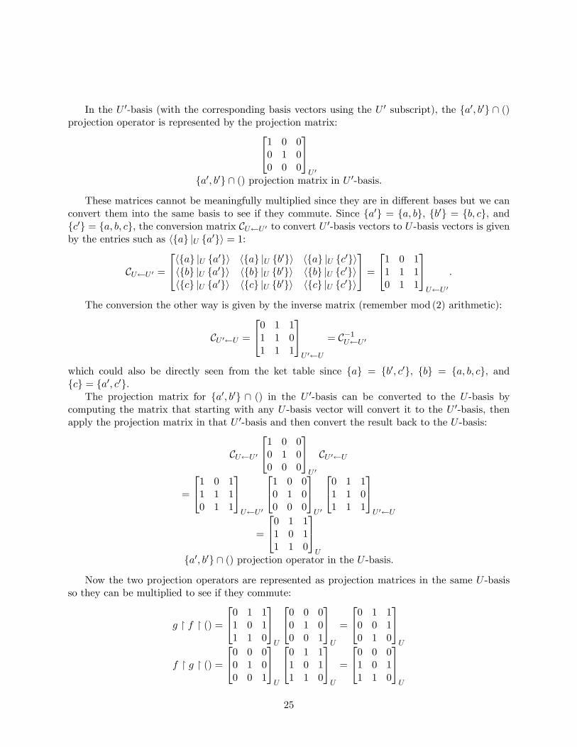
Now the two projection operators are represented as projection matrices in the same U -basisso they can be multiplied to see if they commute:

g � f � () =

0 1 11 0 11 1 0

U

0 0 00 1 00 0 1

U

=

0 1 10 0 10 1 0

U

f � g � () =

0 0 00 1 00 0 1

U

0 1 11 0 11 1 0

U

=

0 0 01 0 11 1 0

U

25

so the two projection matrices do not commute, as we previously saw in the table computation.There is a standard theorem of linear algebra:

Proposition 2 For two diagonalizable (i.e., eigenvectors span the space) linear operators on afinite dimensional space: the operators commute if and only if there is a basis of simultaneouseigenvectors [17, p. 177].

In the above example of non-commuting projection operators, there is no basis of simultaneouseigenvectors (in fact {b, c} = {b′} is the only common eigenvector).

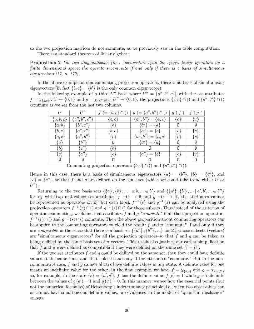
In the following example of a third U ′′-basis where U ′′ = {a′′, b′′, c′′} with the set attributesf = χ{b,c} : U → {0, 1} and g = χ{a′′,b′′} : U ′′ → {0, 1}, the projections {b, c} ∩ () and {a′′, b′′} ∩ ()commute as we see from the last two columns.

U U ′′ f �= {b, c} ∩ () g �= {a′′, b′′} ∩ () g � f � f � g �{a, b, c} {a′′, b′′, c′′} {b, c} {a′′, b′′} = {a, c} {c} {c}{a, b} {b′′, c′′} {b} {b′′} = {a} ∅ ∅{b, c} {a′′, c′′} {b, c} {a′′} = {c} {c} {c}{a, c} {a′′, b′′} {c} {a′′, b′′} = {a, c} {c} {c}{a} {b′′} 0 {b′′} = {a} ∅ ∅{b} {c′′} {b} ∅ ∅ ∅{c} {a′′} {c} {a′′} = {c} {c} {c}∅ ∅ 0 0 0 0

Commuting projection operators {b, c} ∩ () and {a′′, b′′} ∩ ().

Hence in this case, there is a basis of simultaneous eigenvectors {a} = {b′′}, {b} = {c′′}, and{c} = {a′′}, so that f and g are defined on the same set (which we could take to be either U orU ′′).

Returning to the two basis sets {{a} , {b} , ... | a, b, ... ∈ U} and {{a′} , {b′} , ... | a′, b′, ... ∈ U ′}for Zn2 with two real-valued set attributes f : U → R and g : U ′ → R, the attributes cannotbe represented as operators on Zn2 but each block f−1 (r) and g−1 (s) can be analyzed using theprojection operators f−1 (r) ∩ () and g−1 (s) ∩ () for those subsets. Thus instead of the criterion ofoperators commuting, we define that attributes f and g "commute" if all their projection operatorsf−1 (r)∩ () and g−1 (s)∩ () commute. Then the above proposition about commuting operators canbe applied to the commuting operators to yield the result: f and g "commute" if and only if theyare compatible in the sense that there is a basis set {{a′′} , {b′′} , ...} for Zn2 whose subsets (vectors)are "simultaneous eigenvectors" for all the projection operators—so that f and g can be taken asbeing defined on the same basis set of n vectors. This result also justifies our earlier simplificationthat f and g were defined as compatible if they were defined on the same set U = U ′.

If the two set attributes f and g could be defined on the same set, then they could have definitevalues at the same time, and that holds if and only if the attributes "commute." But in the non-commutative case, f and g cannot always have definite values in any state. A definite value for onemeans an indefinite value for the other. In the first example, we have f = χ{b,c} and g = χ{a′,b′}so, for example, in the state {c} = {a′, c′}, f has the definite value f (c) = 1 while g is indefinitebetween the values of g (a′) = 1 and g (c′) = 0. In this manner, we see how the essential points (butnot the numerical formulas) of Heisenberg’s indeterminacy principle, i.e., when two observables canor cannot have simultaneous definite values, are evidenced in the model of "quantum mechanics"on sets.

26

6.4 Entanglement in "quantum mechanics" on sets

Another QM concept that also generates much mystery is entanglement. Hence it might be usefulto consider entanglement in "quantum mechanics" on sets.

First we need to lift the set notion of the direct (or Cartesian) product X × Y of two sets Xand Y . Using the basis principle, we apply the set concept to the two basis sets {v1, ..., vm} and{w1, ..., wn} of two vector spaces V and W (over the same base field) and then we see what itgenerates. The set direct product of the two basis sets is the set of all ordered pairs (vi, wj), whichwe will write as vi ⊗ wj , and then we generate the vector space, denoted V ⊗W , over the samebase field from those basis elements vi ⊗ wj . That vector space is the tensor product, and it notthe direct product V ×W of the vector spaces. The cardinality of X × Y is the product of thecardinalities of the two sets, and the dimension of the tensor product V ⊗W is the product of thedimensions of the two spaces (while the dimension of the direct product V ×W is the sum of thetwo dimensions).

A vector z ∈ V ⊗W is said to be separated if there are vectors v ∈ V and w ∈ W such thatz = v⊗w; otherwise, z is said to be entangled. Since vectors delift to subsets, a subset S ⊆ X × Yis said to be "separated" or a product if there exists subsets SX ⊆ X and SY ⊆ Y such thatS = SX ×SY ; otherwise S ⊆ X × Y is said to be "entangled." In general, let SX be the support orprojection of S on X, i.e., SX = {x : ∃y ∈ Y, (x, y) ∈ S} and similarly for SY . Then S is "separated"iff S = SX × SY .

For any subset S ⊆ X × Y , where X and Y are finite sets, a natural measure of its "entangle-ment" can be constructed by first viewing S as the support of the equiprobable or Laplacian jointprobability distribution on S. If |S| = N , then define Pr (x, y) = 1

N if (x, y) ∈ S and Pr (x, y) = 0otherwise.

The marginal distributions17 are defined in the usual way:

Pr (x) =∑

y Pr (x, y)Pr (y) =

∑x Pr (x, y).

A joint probability distribution Pr (x, y) on X × Y is independent if for all (x, y) ∈ X × Y ,

Pr (x, y) = Pr (x) Pr (y).Independent distribution

Otherwise Pr (x, y) is said to be correlated.

Proposition 3 A subset S ⊆ X × Y is "entangled" iff the equiprobable distribution on S is corre-lated.

Proof: If S is "separated", i.e., S = SX × SY , then Pr (x) = |SY |/N for x ∈ SX and Pr (y) =|SX | /N for y ∈ SY where |SX | |SY | = N . Then for (x, y) ∈ S,

Pr (x, y) = 1N = N

N2 = |SX ||SY |N2 = Pr (x) Pr (y)

17The marginal distributions are the set versions of the reduced density matrices of QM.

27

and Pr(x, y) = 0 = Pr (x) Pr (y) for (x, y) /∈ S so the equiprobable distribution is independent.If S is "entangled," i.e., S 6= SX × SY , then S $ SX × SY so let (x, y) ∈ SX × SY − S. ThenPr (x) ,Pr (y) > 0 but Pr (x, y) = 0 so it is not independent, i.e., is correlated. �

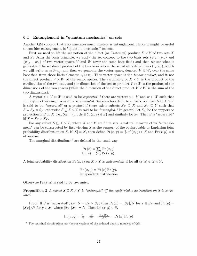
Consider the set version of one qubit space where U = {a, b}. The product set U × U has 15nonempty subsets. Each factor U and U has 3 nonempty subsets so 3× 3 = 9 of the 15 subsets are"separated" subsets leaving 6 "entangled" subsets.

S ⊆ U × U{(a, a) , (b, b)}{(a, b) , (b, a)}

{(a, a) , (a, b), (b, a)}{(a, a) , (a, b), (b, b)}{(a, b), (b, a) , (b, b)}{(a, a), (b, a) , (b, b)}

The six entangled subsets

The first two are the "Bell states" which are the two graphs of bijections U ←→ U and have themaximum entanglement if entanglement is measured by the logical divergence d (Pr(x, y)||Pr (x) Pr (y))[8].All the 9 "separated" states have zero "entanglement" by the same measure.

For an "entangled" subset S, a sampling x of left-hand system will change the probabilitydistribution for a sampling of the right-hand system y, Pr (y|x) 6= Pr (y). In the case of maximal"entanglement" (e.g., the "Bell states"), when S is the graph of a bijection between U and U , thevalue of y is determined by the value of x (and vice-versa).

In this manner, we see that many of the basic ideas and relationships of quantum mechanicalentanglement (e.g., "entangled states," "reduced density matrices," maximally "entangled states,"and "Bell states"), can be reproduced in "quantum mechanics" on sets.

The two-slit experiment and the Bell inequality for "quantum mechanics" on sets are developedin Appendices 2 and 3.

7 Waving good-by to waves

7.1 Wave-particle duality = indistinct-distinct particle duality

States that are indistinct for an observable are represented as weighted vector sums or superpositionsof the eigenstates that might be actualized by further distinctions. This indistinctness-represented-as-superpositions is usually interpreted as "wave-like aspects" of the particles in the indefinitestate. Hence the distinction-making measurements take away the indistinctness—which is usuallyinterpreted as taking away the "wave-like aspects," i.e., "collapse of the wave packet." But thereare no actual physical waves in quantum mechanics (e.g., the "wave amplitudes" are complexnumbers); only particles with indistinct attributes for certain observables. Thus the "collapse ofthe wave packet" is better described as the "collapse of indefiniteness" to achieve definiteness. Andthe "wave-particle duality" is actually the indistinct-distinct particle duality or complementarity.

We have provided the back-story to objective indefiniteness by building the notion of distinctionsfrom the ground up starting with partition logic and logical information theory. But the importanceof distinctions and indistinguishability has been there all along in quantum mechanics.

28

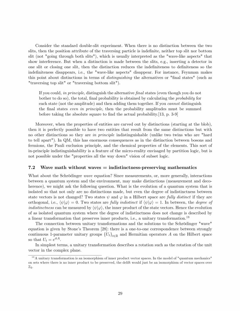
Consider the standard double-slit experiment. When there is no distinction between the twoslits, then the position attribute of the traversing particle is indefinite, neither top slit nor bottomslit (not "going through both slits"), which is usually interpreted as the "wave-like aspects" thatshow interference. But when a distinction is made between the slits, e.g., inserting a detector inone slit or closing one slit, then the distinction reduces the indefiniteness to definiteness so theindefiniteness disappears, i.e., the "wave-like aspects" disappear. For instance, Feynman makesthis point about distinctions in terms of distinguishing the alternatives or "final states" (such as"traversing top slit" or "traversing bottom slit").

If you could, in principle, distinguish the alternative final states (even though you do notbother to do so), the total, final probability is obtained by calculating the probability foreach state (not the amplitude) and then adding them together. If you cannot distinguishthe final states even in principle, then the probability amplitudes must be summedbefore taking the absolute square to find the actual probability.[13, p. 3-9]

Moreover, when the properties of entities are carved out by distinctions (starting at the blob),then it is perfectly possible to have two entities that result from the same distinctions but withno other distinctions so they are in principle indistinguishable (unlike two twins who are "hardto tell apart"). In QM, this has enormous consequences as in the distinction between bosons andfermions, the Pauli exclusion principle, and the chemical properties of the elements. This sort ofin-principle indistinguishability is a feature of the micro-reality envisaged by partition logic, but isnot possible under the "properties all the way down" vision of subset logic.

7.2 Wave math without waves = indistinctness-preserving mathematics

What about the Schrödinger wave equation? Since measurements, or, more generally, interactionsbetween a quantum system and the environment, may make distinctions (measurement and deco-herence), we might ask the following question. What is the evolution of a quantum system that isisolated so that not only are no distinctions made, but even the degree of indistinctness betweenstate vectors is not changed? Two states ψ and ϕ in a Hilbert space are fully distinct if they areorthogonal, i.e., 〈ψ|ϕ〉 = 0. Two states are fully indistinct if 〈ψ|ϕ〉 = 1. In between, the degree ofindistinctness can be measured by 〈ψ|ϕ〉, the inner product of the state vectors. Hence the evolutionof as isolated quantum system where the degree of indistinctness does not change is described bya linear transformation that preserves inner products, i.e., a unitary transformation.18

The connection between unitary transformations and the solutions to the Schrödinger "wave"equation is given by Stone’s Theorem [28]: there is a one-to-one correspondence between stronglycontinuous 1-parameter unitary groups {Ut}t∈R and Hermitian operators A on the Hilbert spaceso that Ut = eitA.

In simplest terms, a unitary transformation describes a rotation such as the rotation of the unitvector in the complex plane.

18A unitary transformation is an isomorphism of inner product vector spaces. In the model of "quantum mechanics"on sets where there is no inner product to be preserved, the delift would just be an isomorphism of vector spaces overZ2.

29

Rotating vector

The rotating unit vector traces out the cosine and sine functions on the two axes, and the positionof the arrow can be compactly described as a function of ϕ using Euler’s formula:

eiϕ = cos (ϕ) + i sin (ϕ).

Such complex exponentials and their superpositions are the "wave functions" of QM. The "wavefunctions" describe the evolution of particles in indefinite states in isolated systems where thereare no interactions to change the degree of indistinctness between states, i.e., the context whereSchrödinger’s equation holds. Previously it has been assumed that the mathematics of waves mustdescribe physical waves of some sort, and thus the puzzlement about the "waves" of QM having com-plex amplitudes and no corresponding physical waves. But we have supplied another interpretation;wave mathematics is the mathematics of indefiniteness, e.g., superposition represents indefinitenessand unitary evolution represents the indistinctness-preserving evolution of an isolated system. Thusthe objective indefiniteness approach to interpreting QM provides an explanation for the appear-ance of the wave mathematics (which implies interference as well as the quantized solutions to the"wave" equation that gave QM its name) when, in fact, there are no actual physical waves involved.

8 Logical entropy measures measurement

8.1 Logical entropy as the total distinction probability

The notion of logical entropy of a probability distribution p = (p1, ..., pn), h (p) = 1 −∑

i p2i ,

generalizes to the quantum logical entropy of a density matrix ρ [10],

h (ρ) = 1− tr[ρ2].

Given a state vector |ψ〉 =∑

i αi |i〉 expressed in the orthonormal basis {|i〉}i=1,...,n, the densitymatrix

ρ = |ψ〉 〈ψ| = [ρij ] =[αiα

∗j

](where α∗j is the complex conjugate of αj) is a pure state density matrix. For a pure state densitymatrix:

h (ρ) = 1− tr[ρ2]

= 1−∑

i

∑j αiα

∗jαjα

∗i = 1−

∑i αiα

∗i

∑j αjα

∗j = 1− 1 = 0.

30

Otherwise, a density matrix ρ is said to represent a mixed state, and its logical entropy is positive.In the set case, the logical entropy h (π) of a partition π was interpreted as the probability

that two independent draws from U (equiprobable elements) would give a distinction of π. For aprobability distribution p = (p1, ..., pn), the logical entropy h (p) = 1−

∑i p2i is the probability that

two independent samples from the distribution will give distinct outcomes i 6= j. The probabilityof the distinct outcomes (i, j) for i 6= j is pipj . Since 1 = (p1 + ...+ pn) (p1 + ...+ pn) =

∑i,j pipj ,

we have:

h (p) = 1−∑

i p2i =

∑i,j pipj −

∑i p2i =

∑i 6=j pipj

which is the sum of all the distinction (i.e., distinct indices) probabilities.This interpretation generalizes to the quantum logical entropy h (ρ). The diagonal terms {pi}

in a density matrix:

ρ =

p1 ρ12 · · · ρ1nρ21 p2 · · · ρ2n...

.... . .

...ρn1 ρn2 · · · pn

are the probabilities of getting the ith eigenvector |i〉 in a projective measurement of a system in thestate ρ (using {|i〉} as the measurement basis). The off-diagonal terms ρij give the amplitude thatthe eigenstates |i〉 and |j〉 cohere, i.e., are indistinct, in the state ρ so the absolute square |ρij |2 isthe indistinction probability. Since pipj is the probability of getting |i〉 and |j〉 in two independentmeasurements, the difference pipj − |ρij |2, is the distinction probability. But 1 =

∑i,j pipj so we see

that the interpretation of the logical entropy as the total distinction probability carries over to thequantum case:

h (ρ) = 1− tr[ρ2]

= 1−∑

ij |ρij |2 =

∑ij

[pipj − |ρij |2

]=∑

i 6=j

[pipj − |ρij |2

]Quantum logical entropy = sum of distinction probabilities

where the last step follows since pipi − |ρii|2 = 0.

8.2 Measuring measurement

Since h (ρ) = 0 for a pure state ρ, that means that all the eigenstates |i〉 and |j〉 cohere together, i.e.,are indistinct, in a pure state, like the indiscrete partition or blob in the set case. For set partitions,the transition, 0 → 1, from the blob to the discrete partition turns all the indistinctions (u, u′)(where u 6= u′) into distinctions, and the logical entropy increases from 0 to 1 −

∑i p2i = 1 − 1

nwhere pi = 1

n for |U | = n.Similarly in quantum mechanics, a nondegenerate measurement turns a pure state density

matrix ρ into the mixed state diagonal matrix ρ̂ with the same diagonal entries p1, ..., pn:

ρ =

p1 ρ12 · · · ρ1nρ21 p2 · · · ρ2n...

.... . .

...ρn1 ρn2 · · · pn

measurement⇒ ρ̂ =

p1 0 · · · 00 p2 · · · 0...

.... . .

...0 0 · · · pn

.

31

Hence the quantum logical entropy similarly goes from h (ρ) = 0 to h (ρ̂) = 1−∑

i p2i . This is usually

described by saying that all the off-diagonal coherence terms are decohered in a nondegeneratemeasurement—which means that all the indistinctions (|i〉 , |j〉) where |i〉 6= |j〉 of the pure state(like a mini-blob) are distinguished by the measurement. And the sum of all those new distinctionprobabilities for the decohered off-diagonal terms is precisely the quantum logical entropy since

h (ρ̂) =∑

i 6=j

[pipj − |ρ̂ij |2

]=∑

i 6=j pipj . For any measurement (degenerate or not), the increase in

logical entropy

h (ρ̂)− h (ρ) =∑

new |ρij |2 = sum of new distinction probabilities

where the sum is over the zeroed or decohered coherence terms |ρij |2 that gave indistinction prob-abilities in the pure state ρ. Thus we see how quantum logical entropy interprets the off-diagonalentries in the pure state density matrices and how the change in the quantum logical entropymeasures precisely the decoherence, i.e., the distinctions, made by a measurement.19

9 Lifting to the axioms of quantum mechanics

We have now reached the point where the program of lifting partition logic and logical informa-tion theory to the quantum concepts of Hilbert spaces essentially yields the axioms of quantummechanics.

Using axioms based on [21], the first axiom gives the vector space endpoint of the lifting program.Axiom 1: An isolated system is represented by a complex inner product vector space (i.e., a

Hilbert space) where the complete description of a state of the system is given by a state vector, aunit vector in the system’s space.

Two fully distinct states would be orthogonal (thinking of them as eigenstates of an observable),and a state indefinite between them would be represented as a weighted vector sum or superpositionof the two states.

We previously saw that the evolution of a closed system that preserves the degree of indistinctionbetween states would be a unitary transformation.

Axiom 2: The evolution of a closed quantum system is described by a unitary transformation.In the last section, we saw how a projective measurement would zero some or all of the off-

diagonal coherence terms in a pure state ρ to give a mixed state ρ̂ (and how the sum of the absolutesquares of the zeroed coherence terms gave the change in quantum logical entropy).

Axiom 3: A projective measurement for an observable (Hermitian operator) M =∑

mmPm(spectral decomposition using projection operators Pm) on a pure state ρ has an outcome m withprobability pm = ρmm giving the mixed state ρ̂ =

∑m PmρPm.

And finally we saw how the lifting program lifted the notion of combining sets with the directproduct of sets X × Y to the notion of representing combined quantum systems with the vectorspace generated by taking the direct product of two bases of the state spaces.

Axiom 4: The state space of a composite system is the tensor product of the state spaces of thecomponent systems.

19 In contrast, the standard notion of entropy currently used in quantum information theory, the von Neumannentropy, is only qualitatively related to measurement, i.e., projective measurement increases von Neumann entropy[21, p. 515].

32

10 Conclusion

The objective indefiniteness interpretation of quantum mechanics is based on using partition logic,logical information theory, and the lifting program to fill out the back story to the old notion of"objective indefiniteness" ([25], [26]). In Appendix 1, the lifting program is further applied to liftset representations of groups to vector space representations, and thus to explain the fundamentalimportance of group representation theory in quantum mechanics (not to mention particle physics).But enough of the research program has already been presented to point to some conclusions.

At the level of sets, if we start with a universe set U as representing our common-sense macro-scopic world, then there are only two logics, the logics of subsets and quotient sets (i.e., partitions),to envisage the "creation story" for U . Increase the size of subsets or increase the refinement ofquotient sets until reaching the universe U . That is, starting with the empty subset of U , takelarger and larger subsets of well-defined fully definite elements until finally reaching all the fullydefinite elements of U . Or starting with the indiscrete partition on U , take more and more refinedpartitions, each block interpreted as an indefinite element, until finally reaching all the fully definiteelements of U . Those are the two dual options.

Classical mechanics was fully compatible with the subset creation story, where elements werealways fully propertied ("properties all the way down"). But almost from the beginning, quantummechanics was seen not to be compatible with that world view of always fully definite entities; QMseems to envisage entities at the micro-level that are objectively indefinite. Within the frameworkof the two logics given by subset-partition duality, the "obvious" thing to do is to elaborate on thedual creation story to try to build the other interpretation of QM.

With the development of the logic of partitions (dual to the logic of subsets) and logical in-formation theory built on top of it, the foundation was in place to lift those set concepts to thericher mathematical environment of vector spaces (Hilbert spaces in particular). In that manner,the other interpretation of QM was constructed. Unlike the interpretation based on entities withfully definite properties expressed by Boolean subset logic, the dual interpretation works. That is,the result reproduces the basic ideas and mathematical machinery of quantum mechanics, e.g., asexpressed in four axioms given above. That completes an outline of the vision of micro-reality thatprovides the objective indefiniteness interpretation of quantum mechanics.

11 Appendix 1: Lifting in group representation theory

11.1 Group representations define partitions

Given a set G of mappings R = {Rg : U → U}g∈G on a set U , what are the conditions on the setof mappings so that it is a set representation of a group? Define the binary relation on U × U :

u ∼ u′ if ∃g ∈ G such that Rg (u) = u′.

Then the conditions that make R into a group representation are the conditions that imply u ∼ u′

is an equivalence relation:

1. existence of the identity 1U ∈ U implies reflexivity of ∼;

2. existence of inverses implies symmetry of ∼; and

33

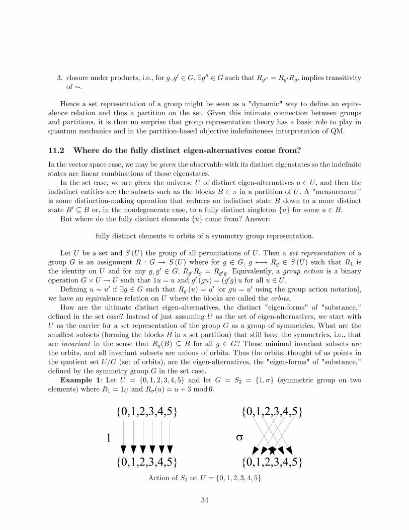
3. closure under products, i.e., for g, g′ ∈ G, ∃g′′ ∈ G such that Rg′′ = Rg′Rg, implies transitivityof ∼.

Hence a set representation of a group might be seen as a "dynamic" way to define an equiv-alence relation and thus a partition on the set. Given this intimate connection between groupsand partitions, it is then no surprise that group representation theory has a basic role to play inquantum mechanics and in the partition-based objective indefiniteness interpretation of QM.

11.2 Where do the fully distinct eigen-alternatives come from?

In the vector space case, we may be given the observable with its distinct eigenstates so the indefinitestates are linear combinations of those eigenstates.

In the set case, we are given the universe U of distinct eigen-alternatives u ∈ U , and then theindistinct entities are the subsets such as the blocks B ∈ π in a partition of U . A "measurement"is some distinction-making operation that reduces an indistinct state B down to a more distinctstate B′ ⊆ B or, in the nondegenerate case, to a fully distinct singleton {u} for some u ∈ B.

But where do the fully distinct elements {u} come from? Answer:

fully distinct elements ≈ orbits of a symmetry group representation.

Let U be a set and S (U) the group of all permutations of U . Then a set representation of agroup G is an assignment R : G → S (U) where for g ∈ G, g 7−→ Rg ∈ S (U) such that R1 isthe identity on U and for any g, g′ ∈ G, Rg′Rg = Rg′g. Equivalently, a group action is a binaryoperation G× U → U such that 1u = u and g′ (gu) = (g′g)u for all u ∈ U .

Defining u ∼ u′ if ∃g ∈ G such that Rg (u) = u′ [or gu = u′ using the group action notation],we have an equivalence relation on U where the blocks are called the orbits.

How are the ultimate distinct eigen-alternatives, the distinct "eigen-forms" of "substance,"defined in the set case? Instead of just assuming U as the set of eigen-alternatives, we start withU as the carrier for a set representation of the group G as a group of symmetries. What are thesmallest subsets (forming the blocks B in a set partition) that still have the symmetries, i.e., thatare invariant in the sense that Rg(B) ⊆ B for all g ∈ G? Those minimal invariant subsets arethe orbits, and all invariant subsets are unions of orbits. Thus the orbits, thought of as points inthe quotient set U/G (set of orbits), are the eigen-alternatives, the "eigen-forms" of "substance,"defined by the symmetry group G in the set case.

Example 1: Let U = {0, 1, 2, 3, 4, 5} and let G = S2 = {1, σ} (symmetric group on twoelements) where R1 = 1U and Rσ(u) = u+ 3 mod 6.

Action of S2 on U = {0, 1, 2, 3, 4, 5}

34

There are 3 orbits: {0, 3} , {1, 4}, and {2, 5}. Those three orbits are the "points" in the quotientset U/G, i.e., they are the distinct eigen-alternatives defined by the symmetry group’s S2 action onU .

A vector space representation of a group G on a vector space V is a mapping g 7−→ Rg : V → Vfrom G to invertible linear transformations on V such that Rg′Rg = Rg′g.

The lifts to the vector space representations of groups are;

• minimal invariant subset = orbits Lifts−→ minimal invariant subspaces = irreducible subspaces,

• representation restricted to orbits Lifts−→ representation restricted to irreducible subspaceswhich gives the irreducible representations (the eigen-forms of substance in the vector spacecase20), and

• set partition of orbits Lifts−→ vector space partition of irreducible subspaces.

The "irreducible representations" in the set case are just the restrictions of the representationto the orbits, e.g., R � {0, 3} : S2 → S ({0, 3}), as their carriers. A set representation is said to betransitive, if for any u, u′ ∈ U , ∃g ∈ G such that Rg (u) = u′. A transitive set representation hasonly one orbit, all of U . Any set "irreducible representation" is transitive.

We are accustomed to thinking of some distinction-making operation as reducing a whole parti-tion to a more refined partition, and thus breaking up a block B into distinguishable non-overlappingsubsets B′, B′′, ... ⊆ B. Now we are working at the more basic level of determining the distinct eigen-alternatives, i.e., the orbits of a set representation of a symmetry group. Here we might also considerhow distinctions are made to move to a more refined partition of orbits. Since the group operationsidentify elements, u ∼ u′ if ∃g ∈ G such that Rg (u) = u′, we would further distinguish elements bymoving to a subgroup. The symmetry operations in the larger group are "broken," so the remaininggroup of symmetries is a subgroup.

Example 1 revisited: the group S2 has only one subgroup, the trivial subgroup of the identityoperation, and its orbits are clearly the singletons {u} for u ∈ U . That is the simplest example ofsymmetry-breaking that gives a more distinct set of eigen-alternatives.

In any set representation, the maximum distinctions are made by the smallest symmetry sub-group which is always the identity subgroup, so that is always the waste case that takes us back tothe singleton orbits in U , i.e., the distinct elements of U .

Thus we see that symmetry-breaking is analogous to measurement but at this more fundamentallevel where the distinct eigen-forms are determined in the first place by symmetry considerations.

20For a certain group of particle physics, "an elementary particle ‘is’an irreducible unitary representation of thegroup."[27, p. 149] In Heisenberg’s philosophical terms, the irreducible representations of certain symmetry groupsof particle physics determine the fundamental eigen-forms that the substance (energy) can take.

The elementary particles are therefore the fundamental forms that the substance energy must take inorder to become matter, and these basic forms must in some way be determined by a fundamental lawexpressible in mathematical terms. ... The real conceptual core of the fundamental law must, however, beformed by the mathematical properties of the symmetry it represents.[16, pp. 16-17]

35

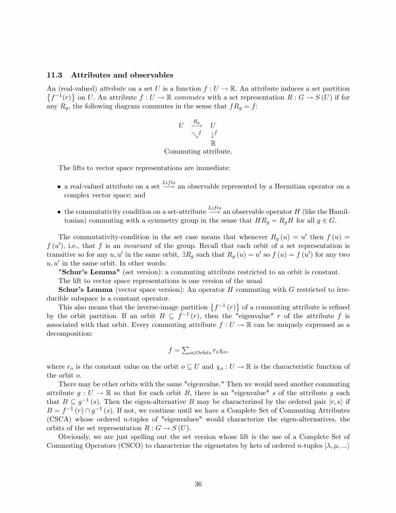
11.3 Attributes and observables

An (real-valued) attribute on a set U is a function f : U → R. An attribute induces a set partition{f−1(r)

}on U . An attribute f : U → R commutes with a set representation R : G→ S (U) if for

any Rg, the following diagram commutes in the sense that fRg = f :

URg−→ U↘f ↓f

RCommuting attribute.

The lifts to vector space representations are immediate:

• a real-valued attribute on a set Lifts−→ an observable represented by a Hermitian operator on acomplex vector space; and

• the commutativity condition on a set-attribute Lifts−→ an observable operatorH (like the Hamil-tonian) commuting with a symmetry group in the sense that HRg = RgH for all g ∈ G.

The commutativity-condition in the set case means that whenever Rg (u) = u′ then f (u) =f (u′), i.e., that f is an invariant of the group. Recall that each orbit of a set representation istransitive so for any u, u′ in the same orbit, ∃Rg such that Rg (u) = u′ so f (u) = f (u′) for any twou, u′ in the same orbit. In other words:

"Schur’s Lemma" (set version): a commuting attribute restricted to an orbit is constant.The lift to vector space representations is one version of the usualSchur’s Lemma (vector space version): An operator H commuting with G restricted to irre-

ducible subspace is a constant operator.This also means that the inverse-image partition

{f−1 (r)

}of a commuting attribute is refined

by the orbit partition. If an orbit B ⊆ f−1 (r), then the "eigenvalue" r of the attribute f isassociated with that orbit. Every commuting attribute f : U → R can be uniquely expressed as adecomposition:

f =∑

o∈Orbits roχo,

where ro is the constant value on the orbit o ⊆ U and χo : U → R is the characteristic function ofthe orbit o.

There may be other orbits with the same "eigenvalue." Then we would need another commutingattribute g : U → R so that for each orbit B, there is an "eigenvalue" s of the attribute g suchthat B ⊆ g−1 (s). Then the eigen-alternative B may be characterized by the ordered pair |r, s〉 ifB = f−1 (r) ∩ g−1 (s). If not, we continue until we have a Complete Set of Commuting Attributes(CSCA) whose ordered n-tuples of "eigenvalues" would characterize the eigen-alternatives, theorbits of the set representation R : G→ S (U).

Obviously, we are just spelling out the set version whose lift is the use of a Complete Set ofCommuting Operators (CSCO) to characterize the eigenstates by kets of ordered n-tuples |λ, µ, ...〉

36

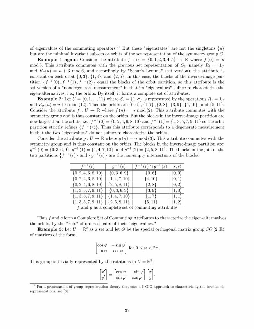
of eigenvalues of the commuting operators.21 But these "eigenstates" are not the singletons {u}but are the minimal invariant subsets or orbits of the set representation of the symmetry group G.

Example 1 again: Consider the attribute f : U = {0, 1, 2, 3, 4, 5} → R where f (n) = nmod 3. This attribute commutes with the previous set representation of S2, namely R1 = 1Uand Rσ(u) = u + 3 mod 6, and accordingly by "Schur’s Lemma" (set version), the attribute isconstant on each orbit {0, 3} , {1, 4}, and {2, 5}. In this case, the blocks of the inverse-image par-tition

{f−1 (0) , f−1 (1) , f−1 (2)

}equal the blocks of the orbit partition, so this attribute is the

set version of a "nondegenerate measurement" in that its "eigenvalues" suffi ce to characterize theeigen-alternatives, i.e., the orbits. By itself, it forms a complete set of attributes.

Example 2: Let U = {0, 1, ..., 11} where S2 = {1, σ} is represented by the operations R1 = 1Uand Rσ (n) = n+ 6 mod (12). Then the orbits are {0, 6} , {1, 7} , {2, 8} , {3, 9} , {4, 10} , and {5, 11}.Consider the attribute f : U → R where f (n) = n mod (2). This attribute commutes with thesymmetry group and is thus constant on the orbits. But the blocks in the inverse-image partition arenow larger than the orbits, i.e., f−1 (0) = {0, 2, 4, 6, 8, 10} and f−1 (1) = {1, 3, 5, 7, 9, 11} so the orbitpartition strictly refines

{f−1 (r)

}. Thus this attribute corresponds to a degenerate measurement

in that the two "eigenvalues" do not suffi ce to characterize the orbits.Consider the attribute g : U → R where g (n) = n mod (3). This attribute commutes with the

symmetry group and is thus constant on the orbits. The blocks in the inverse-image partition are:g−1 (0) = {0, 3, 6, 9}, g−1 (1) = {1, 4, 7, 10}, and g−1 (2) = {2, 5, 8, 11}. The blocks in the join of thetwo partitions

{f−1 (r)

}and

{g−1 (s)

}are the non-empty intersections of the blocks:

f−1 (r) g−1 (s) f−1 (r) ∩ g−1 (s) |r, s〉{0, 2, 4, 6, 8, 10} {0, 3, 6, 9} {0, 6} |0, 0〉{0, 2, 4, 6, 8, 10} {1, 4, 7, 10} {4, 10} |0, 1〉{0, 2, 4, 6, 8, 10} {2, 5, 8, 11} {2, 8} |0, 2〉{1, 3, 5, 7, 9, 11} {0, 3, 6, 9} {3, 9} |1, 0〉{1, 3, 5, 7, 9, 11} {1, 4, 7, 10} {1, 7} |1, 1〉{1, 3, 5, 7, 9, 11} {2, 5, 8, 11} {5, 11} |1, 2〉f and g as a complete set of commuting attributes

Thus f and g form a Complete Set of Commuting Attributes to characterize the eigen-alternatives,the orbits, by the "kets" of ordered pairs of their "eigenvalues."

Example 3: Let U = R2 as a set and let G be the special orthogonal matrix group SO (2,R)of matrices of the form; [

cosϕ − sinϕsinϕ cosϕ

]for 0 ≤ ϕ < 2π.

This group is trivially represented by the rotations in U = R2:[x′

y′

]=

[cosϕ − sinϕsinϕ cosϕ

] [xy

].

21For a presentation of group representation theory that uses a CSCO approach to characterizing the irreduciblerepresentations, see [3].

37

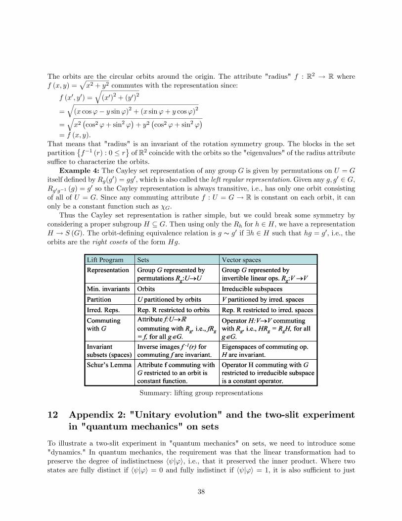
The orbits are the circular orbits around the origin. The attribute "radius" f : R2 → R wheref (x, y) =

√x2 + y2 commutes with the representation since:

f (x′, y′) =√

(x′)2 + (y′)2

=√

(x cosϕ− y sinϕ)2 + (x sinϕ+ y cosϕ)2

=√x2(cos2 ϕ+ sin2 ϕ

)+ y2

(cos2 ϕ+ sin2 ϕ

)= f (x, y).

That means that "radius" is an invariant of the rotation symmetry group. The blocks in the setpartition

{f−1 (r) : 0 ≤ r

}of R2 coincide with the orbits so the "eigenvalues" of the radius attribute

suffi ce to characterize the orbits.Example 4: The Cayley set representation of any group G is given by permutations on U = G

itself defined by Rg(g′) = gg′, which is also called the left regular representation. Given any g, g′ ∈ G,Rg′g−1 (g) = g′ so the Cayley representation is always transitive, i.e., has only one orbit consistingof all of U = G. Since any commuting attribute f : U = G → R is constant on each orbit, it canonly be a constant function such as χG.

Thus the Cayley set representation is rather simple, but we could break some symmetry byconsidering a proper subgroup H ⊆ G. Then using only the Rh for h ∈ H, we have a representationH → S (G). The orbit-defining equivalence relation is g ∼ g′ if ∃h ∈ H such that hg = g′, i.e., theorbits are the right cosets of the form Hg.

Summary: lifting group representations

12 Appendix 2: "Unitary evolution" and the two-slit experimentin "quantum mechanics" on sets

To illustrate a two-slit experiment in "quantum mechanics" on sets, we need to introduce some"dynamics." In quantum mechanics, the requirement was that the linear transformation had topreserve the degree of indistinctness 〈ψ|ϕ〉, i.e., that it preserved the inner product. Where twostates are fully distinct if 〈ψ|ϕ〉 = 0 and fully indistinct if 〈ψ|ϕ〉 = 1, it is also suffi cient to just

38

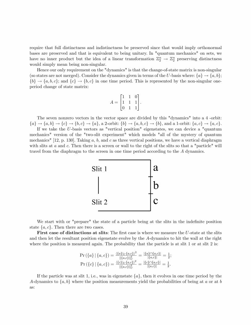
require that full distinctness and indistinctness be preserved since that would imply orthonormalbases are preserved and that is equivalent to being unitary. In "quantum mechanics" on sets, wehave no inner product but the idea of a linear transformation Zn2 → Zn2 preserving distinctnesswould simply mean being non-singular.

Hence our only requirement on the "dynamics" is that the change-of-state matrix is non-singular(so states are not merged). Consider the dynamics given in terms of the U -basis where: {a} → {a, b};{b} → {a, b, c}; and {c} → {b, c} in one time period. This is represented by the non-singular one-period change of state matrix:

A =

1 1 01 1 10 1 1

.The seven nonzero vectors in the vector space are divided by this "dynamics" into a 4 -orbit:

{a} → {a, b} → {c} → {b, c} → {a}, a 2-orbit: {b} → {a, b, c} → {b}, and a 1-orbit: {a, c} → {a, c}.If we take the U -basis vectors as "vertical position" eigenstates, we can device a "quantum

mechanics" version of the "two-slit experiment" which models "all of the mystery of quantummechanics" [12, p. 130]. Taking a, b, and c as three vertical positions, we have a vertical diaphragmwith slits at a and c. Then there is a screen or wall to the right of the slits so that a "particle" willtravel from the diaphragm to the screen in one time period according to the A dynamics.

We start with or "prepare" the state of a particle being at the slits in the indefinite positionstate {a, c}. Then there are two cases.

First case of distinctions at slits: The first case is where we measure the U -state at the slitsand then let the resultant position eigenstate evolve by the A-dynamics to hit the wall at the rightwhere the position is measured again. The probability that the particle is at slit 1 or at slit 2 is:

Pr ({a} | {a, c}) = 〈{a}|U{a,c}〉2

‖{a,c}‖2U= |{a}∩{a,c}|

|{a,c}| = 12 ;

Pr ({c} | {a, c}) = 〈{c}|U{a,c}〉2

‖{a,c}‖2U= |{c}∩{a,c}|

|{a,c}| = 12 .

If the particle was at slit 1, i.e., was in eigenstate {a}, then it evolves in one time period by theA-dynamics to {a, b} where the position measurements yield the probabilities of being at a or at bas:

39

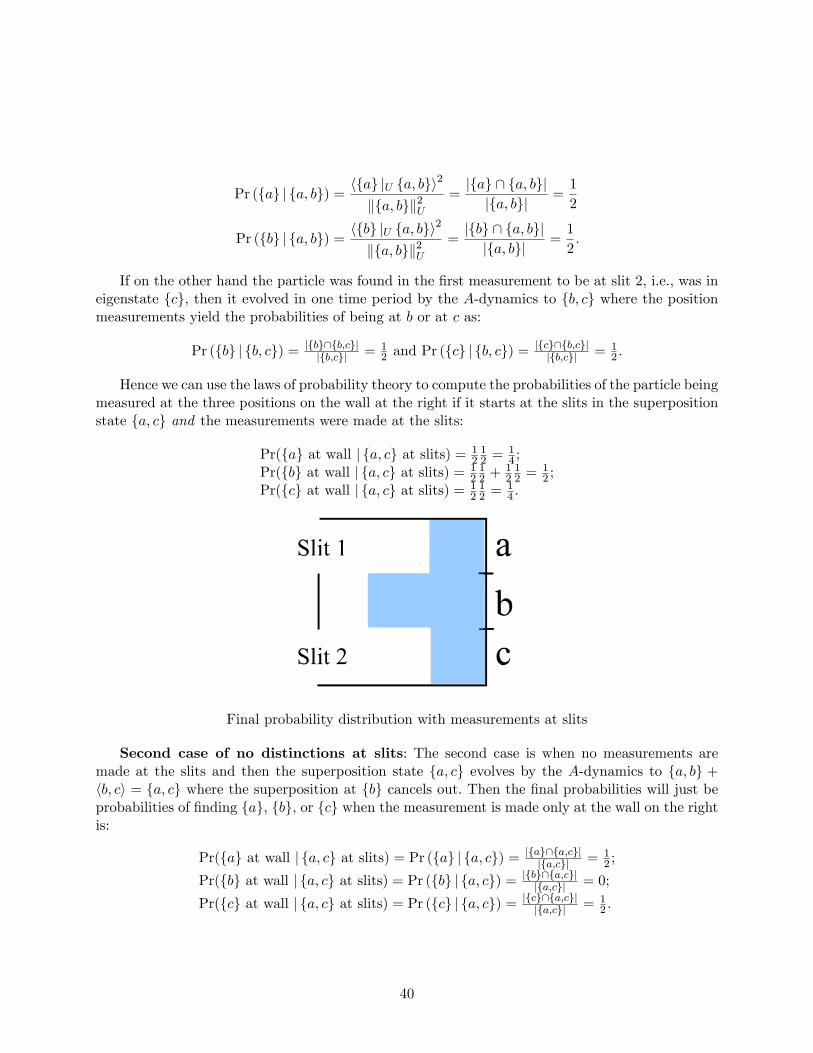
Pr ({a} | {a, b}) =〈{a} |U {a, b}〉2

‖{a, b}‖2U=|{a} ∩ {a, b}||{a, b}| =

1

2

Pr ({b} | {a, b}) =〈{b} |U {a, b}〉2

‖{a, b}‖2U=|{b} ∩ {a, b}||{a, b}| =

1

2.

If on the other hand the particle was found in the first measurement to be at slit 2, i.e., was ineigenstate {c}, then it evolved in one time period by the A-dynamics to {b, c} where the positionmeasurements yield the probabilities of being at b or at c as:

Pr ({b} | {b, c}) = |{b}∩{b,c}||{b,c}| = 1

2 and Pr ({c} | {b, c}) = |{c}∩{b,c}||{b,c}| = 1

2 .

Hence we can use the laws of probability theory to compute the probabilities of the particle beingmeasured at the three positions on the wall at the right if it starts at the slits in the superpositionstate {a, c} and the measurements were made at the slits:

Pr({a} at wall | {a, c} at slits) = 1212 = 1

4 ;Pr({b} at wall | {a, c} at slits) = 1

212 + 1

212 = 1

2 ;Pr({c} at wall | {a, c} at slits) = 1

212 = 1

4 .

Final probability distribution with measurements at slits

Second case of no distinctions at slits: The second case is when no measurements aremade at the slits and then the superposition state {a, c} evolves by the A-dynamics to {a, b} +〈b, c〉 = {a, c} where the superposition at {b} cancels out. Then the final probabilities will just beprobabilities of finding {a}, {b}, or {c} when the measurement is made only at the wall on the rightis:

Pr({a} at wall | {a, c} at slits) = Pr ({a} | {a, c}) = |{a}∩{a,c}||{a,c}| = 1

2 ;

Pr({b} at wall | {a, c} at slits) = Pr ({b} | {a, c}) = |{b}∩{a,c}||{a,c}| = 0;

Pr({c} at wall | {a, c} at slits) = Pr ({c} | {a, c}) = |{c}∩{a,c}||{a,c}| = 1

2 .

40

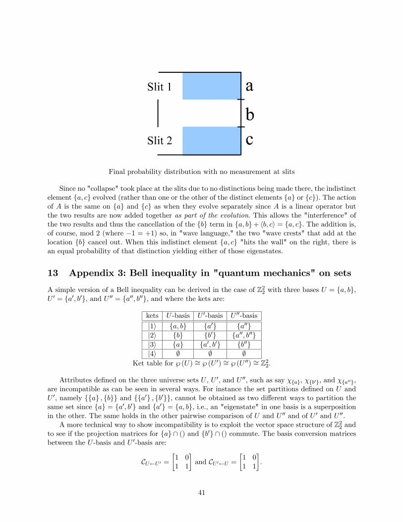
Final probability distribution with no measurement at slits

Since no "collapse" took place at the slits due to no distinctions being made there, the indistinctelement {a, c} evolved (rather than one or the other of the distinct elements {a} or {c}). The actionof A is the same on {a} and {c} as when they evolve separately since A is a linear operator butthe two results are now added together as part of the evolution. This allows the "interference" ofthe two results and thus the cancellation of the {b} term in {a, b}+ 〈b, c〉 = {a, c}. The addition is,of course, mod 2 (where −1 = +1) so, in "wave language," the two "wave crests" that add at thelocation {b} cancel out. When this indistinct element {a, c} "hits the wall" on the right, there isan equal probability of that distinction yielding either of those eigenstates.

13 Appendix 3: Bell inequality in "quantum mechanics" on sets

A simple version of a Bell inequality can be derived in the case of Z22 with three bases U = {a, b},U ′ = {a′, b′}, and U ′′ = {a′′, b′′}, and where the kets are:

kets U -basis U ′-basis U ′′-basis

|1〉 {a, b} {a′} {a′′}|2〉 {b} {b′} {a′′, b′′}|3〉 {a} {a′, b′} {b′′}|4〉 ∅ ∅ ∅

Ket table for ℘ (U) ∼= ℘ (U ′) ∼= ℘ (U ′′) ∼= Z22.

Attributes defined on the three universe sets U , U ′, and U ′′, such as say χ{a}, χ{b′}, and χ{a′′},are incompatible as can be seen in several ways. For instance the set partitions defined on U andU ′, namely {{a} , {b}} and {{a′} , {b′}}, cannot be obtained as two different ways to partition thesame set since {a} = {a′, b′} and {a′} = {a, b}, i.e., an "eigenstate" in one basis is a superpositionin the other. The same holds in the other pairwise comparison of U and U ′′ and of U ′ and U ′′.

A more technical way to show incompatibility is to exploit the vector space structure of Z22 andto see if the projection matrices for {a} ∩ () and {b′} ∩ () commute. The basis conversion matricesbetween the U -basis and U ′-basis are:

CU←U ′ =

[1 01 1

]and CU ′←U =

[1 01 1

].

41

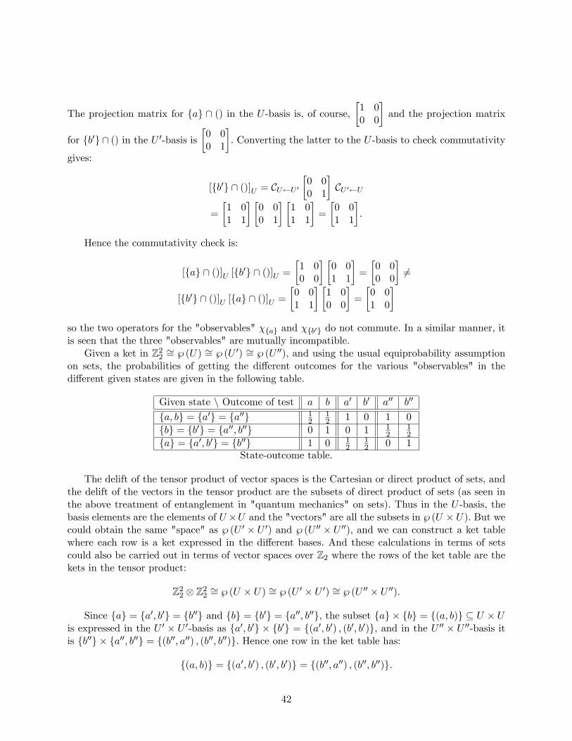
The projection matrix for {a} ∩ () in the U -basis is, of course,[1 00 0

]and the projection matrix

for {b′} ∩ () in the U ′-basis is[0 00 1

]. Converting the latter to the U -basis to check commutativity

gives:

[{b′} ∩ ()]U = CU←U ′[0 00 1

]CU ′←U

=

[1 01 1

] [0 00 1

] [1 01 1

]=

[0 01 1

].

Hence the commutativity check is:

[{a} ∩ ()]U [{b′} ∩ ()]U =

[1 00 0

] [0 01 1

]=

[0 00 0

]6=

[{b′} ∩ ()]U [{a} ∩ ()]U =

[0 01 1

] [1 00 0

]=

[0 01 0

]so the two operators for the "observables" χ{a} and χ{b′} do not commute. In a similar manner, itis seen that the three "observables" are mutually incompatible.

Given a ket in Z22 ∼= ℘ (U) ∼= ℘ (U ′) ∼= ℘ (U ′′), and using the usual equiprobability assumptionon sets, the probabilities of getting the different outcomes for the various "observables" in thedifferent given states are given in the following table.

Given state \ Outcome of test a b a′ b′ a′′ b′′

{a, b} = {a′} = {a′′} 12

12 1 0 1 0

{b} = {b′} = {a′′, b′′} 0 1 0 1 12

12

{a} = {a′, b′} = {b′′} 1 0 12

12 0 1

State-outcome table.

The delift of the tensor product of vector spaces is the Cartesian or direct product of sets, andthe delift of the vectors in the tensor product are the subsets of direct product of sets (as seen inthe above treatment of entanglement in "quantum mechanics" on sets). Thus in the U -basis, thebasis elements are the elements of U ×U and the "vectors" are all the subsets in ℘ (U × U). But wecould obtain the same "space" as ℘ (U ′ × U ′) and ℘ (U ′′ × U ′′), and we can construct a ket tablewhere each row is a ket expressed in the different bases. And these calculations in terms of setscould also be carried out in terms of vector spaces over Z2 where the rows of the ket table are thekets in the tensor product:

Z22 ⊗ Z22 ∼= ℘ (U × U) ∼= ℘ (U ′ × U ′) ∼= ℘ (U ′′ × U ′′).

Since {a} = {a′, b′} = {b′′} and {b} = {b′} = {a′′, b′′}, the subset {a} × {b} = {(a, b)} ⊆ U × Uis expressed in the U ′ × U ′-basis as {a′, b′} × {b′} = {(a′, b′) , (b′, b′)}, and in the U ′′ × U ′′-basis itis {b′′} × {a′′, b′′} = {(b′′, a′′) , (b′′, b′′)}. Hence one row in the ket table has:

{(a, b)} = {(a′, b′) , (b′, b′)} = {(b′′, a′′) , (b′′, b′′)}.

42

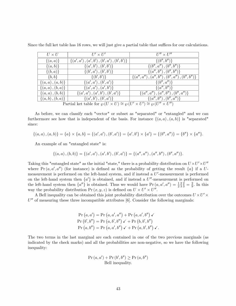
Since the full ket table has 16 rows, we will just give a partial table that suffi ces for our calculations.

U × U U ′ × U ′ U ′′ × U ′′

{(a, a)} {(a′, a′) , (a′, b′) , (b′, a′) , (b′, b′)} {(b′′, b′′)}{(a, b)} {(a′, b′) , (b′, b′)} {(b′′, a′′) , (b′′, b′′)}{(b, a)} {(b′, a′) , (b′, b′)} {(a′′, b′′) , (b′′, b′′)}{b, b} {(b′, b′)} {(a′′, a′′) , (a′′, b′′) , (b′′, a′′) , (b′′, b′′)}

{(a, a) , (a, b)} {(a′, a′) , (b′, a′)} {(b′′, a′′)}{(a, a) , (b, a)} {(a′, a′) , (a′, b′)} {(a′′, b′′)}{(a, a) , (b, b)} {(a′, a′) , (a′, b′) , (b′, a′)} {(a′′, a′′) , (a′′, b′′) , (b′′, a′′)}{(a, b) , (b, a)} {(a′, b′) , (b′, a′)} {(a′′, b′′) , (b′′, a′′)}

Partial ket table for ℘ (U × U) ∼= ℘ (U ′ × U ′) ∼= ℘ (U ′′ × U ′′)

As before, we can classify each "vector" or subset as "separated" or "entangled" and we canfurthermore see how that is independent of the basis. For instance {(a, a) , (a, b)} is "separated"since:

{(a, a) , (a, b)} = {a} × {a, b} = {(a′, a′) , (b′, a′)} = {a′, b′} × {a′} = {(b′′, a′′)} = {b′′} × {a′′}.

An example of an "entangled state" is:

{(a, a) , (b, b)} = {(a′, a′) , (a′, b′) , (b′, a′)} = {(a′′, a′′) , (a′′, b′′) , (b′′, a′′)}.

Taking this "entangled state" as the initial "state," there is a probability distribution on U×U ′×U ′′where Pr (a, a′, a′′) (for instance) is defined as the probability of getting the result {a} if a U -measurement is performed on the left-hand system, and if instead a U ′-measurement is performedon the left-hand system then {a′} is obtained, and if instead a U ′′-measurement is performed onthe left-hand system then {a′′} is obtained. Thus we would have Pr (a, a′, a′′) = 1

22323 = 2

9 . In thisway the probability distribution Pr (x, y, z) is defined on U × U ′ × U ′′.

A Bell inequality can be obtained this joint probability distribution over the outcomes U×U ′×U ′′ of measuring these three incompatible attributes [6]. Consider the following marginals:

Pr(a, a′

)= Pr

(a, a′, a′′

)+ Pr

(a, a′, b′′

)X

Pr(b′, b′′

)= Pr

(a, b′, b′′

)X+ Pr

(b, b′, b′′

)Pr(a, b′′

)= Pr

(a, a′, b′′

)X+ Pr

(a, b′, b′′

)X.

The two terms in the last marginal are each contained in one of the two previous marginals (asindicated by the check marks) and all the probabilities are non-negative, so we have the followinginequality:

Pr (a, a′) + Pr (b′, b′′) ≥ Pr (a, b′′)Bell inequality.

43

All this has to do with measurements on the left-hand system. But there is an alternativeinterpretation to the probabilities Pr (x, y), Pr (y, z), and Pr (x, z) if we assume that the outcomeof a measurement on the right-hand system is independent of the outcome of the same measurementon the left-hand system. Then Pr (a, a′) is the probability of a U -measurement on the left-handsystem giving {a} and then a U ′-measurement on the right-hand system giving {a′}, and so forth.Under that independence assumption and for this initially prepared "Bell state,"

{(a, a) , (b, b)} = {(a′, a′) , (a′, b′) , (b′, a′)} = {(a′′, a′′) , (a′′, b′′) , (b′′, a′′)},

the probabilities would be the same.22 That is, the probabilities, Pr (a) = 12 = Pr (b), Pr (a′) =

23 = Pr (a′′), and Pr (b′) = 1

3 = Pr (b′′) are the same regardless of whether we are measuring theleft-hand or right-hand system of that composite state. Hence the above Bell inequality would stillhold. But we can use "quantum mechanics" on sets to compute the probabilities for those differentmeasurements on the two systems to see if the independence assumption is compatible with "QM"on sets.

To compute Pr (a, a′), we first measure the left-hand component in the U -basis. Since {(a, a) , (b, b)}is the given state, and (a, a) and (b, b) are equiprobable, the probability of getting {a} (i.e., the"eigenvalue" 1 for the "observable χ{a}) is

12 . But the right-hand system is then in the state {a}

and the probability of getting {a′} (i.e., "eigenvalue" 0 for the "observable" χ{b′}) is12 (as seen in

the state-outcome table). Thus the probability is Pr (a, a′) = 1212 = 1

4 .To compute Pr (b′, b′′), we first perform a U ′-basis "measurement" on the left-hand component

of the given state {(a, a) , (b, b)} = {(a′, a′) , (a′, b′) , (b′, a′)}, and we see that the probability ofgetting {b′} is 1

3 . Then the right-hand system is in the state {a′} and the probability of getting{b′′} in a U ′′-basis "measurement" of the right-hand system in the state {a′} is 0 (as seen from thestate-outcome table). Hence the probability is Pr (b′, b′′) = 0.

Finally we compute Pr (a, b′′) by first making a U -measurement on the left-hand component ofthe given state {(a, a) , (b, b)} and get the result {a} with probability 1

2 . Then the state of the secondsystem is {a} so a U ′′-measurement will give the {b′′} result with probability 1 so the probabilityis Pr (a, b′′) = 1

2 .Then we plug the probabilities into the Bell inequality:

Pr (a, a′) + Pr (b′, b′′) ≥ Pr (a, b′′)14 + 0 � 1

2Violation of Bell inequality.

The violation of the Bell inequality shows that the independence assumption about the measurementoutcomes on the left-hand and right-hand systems is incompatible with "QM" on sets so the effectsof the "QM" on sets measurements are "nonlocal."

References

[1] Boole, George 1854. An Investigation of the Laws of Thought on which are founded the Math-ematical Theories of Logic and Probabilities. Cambridge: Macmillan and Co.

22The same holds for the other maximally entangled "Bell state": {(a, b) , (b, a)}.

44

[2] Britz, Thomas, Matteo Mainetti and Luigi Pezzoli 2001. Some operations on the family ofequivalence relations. In Algebraic Combinatorics and Computer Science: A Tribute to Gian-Carlo Rota. Henry Crapo and Domenico Senato eds., Milano: Springer: 445-59.

[3] Chen, Jin-Quan, Jialun Ping and Fan Wang 2002. Group Representation Theory for Physicists(2nd ed.). Singapore: World Scientific.

[4] Church, Alonzo 1956. Introduction to Mathematical Logic. Princeton: Princeton UniversityPress.

[5] Cohen-Tannoudji, Claude, Bernard Diu and Franck Laloë 2005. Quantum Mechanics Vol. 1.New York: John Wiley & Sons.

[6] D’Espagnat, Bernard 1979. The quantum theory and reality. Scientific American. 241 (5):158-181.

[7] Dirac, P. A. M. 1958. The Principles of Quantum Mechanics (4th ed.). Oxford: ClarendonPress.

[8] Ellerman, David 2009. Counting Distinctions: On the Conceptual Foundations of Shannon’sInformation Theory. Synthese. 168 (1 May): 119-149. Downloadable at www.ellerman.org.

[9] Ellerman, David 2010. The Logic of Partitions: Introduction to the Dual of the Logic of Subsets.Review of Symbolic Logic. 3 (2 June): 287-350. Downloadable at www.ellerman.org.

[10] Fano, U. 1957. Description of States in Quantum Mechanics by Density Matrix and OperatorTechniques. Reviews of Modern Physics. 29 (1): 74-93.

[11] Feyerabend, Paul 1983 (orig. 1962). Problems of Microphysics. In Frontiers of Science andPhilosophy. Robert G. Colodny ed., Lanham MD: University Press of America: 189-283.

[12] Feynman, Richard 1967. The Character of Physical Law. Cambridge: MIT Press.

[13] Feynman, Richard P., Robert B. Leighton and Matthew Sands 1965. The Feynman Lectureson Physics: Quantum Mechanics (Vol. III). Reading MA: Addison-Wesley.

[14] Finberg, David, Matteo Mainetti and Gian-Carlo Rota 1996. The Logic of Commuting Equiv-alence Relations. In Logic and Algebra. Aldo Ursini and Paolo Agliano eds., New York: MarcelDekker: 69-96.

[15] Heisenberg, Werner 1958. Physics & Philosophy: The Revolution in Modern Science. New York:Harper Torchbooks.

[16] Heisenberg, Werner 1961. Planck’s discovery and the philosophical problems of atomic physics.In On Modern Physics. New York: Clarkson N. Potter Inc.: 3-19.

[17] Hoffman, Kenneth and Ray Kunze 1961. Linear Algebra. Englewood Cliffs NJ: Prentice-Hall.

[18] Hughes, R.I.G. 1989. The structure and interpretation of quantum mechanics. Cambridge:Harvard University Press.

45

[19] Jammer, Max 1974. The Philosophy of Quantum Mechanics: The Interpretations of QuantumMechanics in Historical Perspective. New York: John Wiley.

[20] Lawvere, F. William and Robert Rosebrugh 2003. Sets for Mathematics. Cambridge: Cam-bridge University Press.

[21] Nielsen, Michael and Isaac Chuang 2000. Quantum Computation and Quantum Information.Cambridge: Cambridge University Press.

[22] Rao, C. R. 1982. Diversity and Dissimilarity Coeffi cients: A Unified Approach. TheoreticalPopulation Biology. 21: 24-43.

[23] Renyi, Alfred 1976 (orig. 1961). A General Method for Proving Theorems in Probability Theoryand Some Applications (Paper 181). In Selected Papers of Alfred Renyi: Vol. 2. Pal Turan ed.,Budapest: Akademiai Kaido: 581-602.

[24] Sakurai, J. J. 2011. Modern Quantum Mechanics. New Delhi: Pearson Educational.

[25] Shimony, Abner 1988. The reality of the quantum world. Scientific American. 258 (1): 46-53.

[26] Shimony, Abner 1989. Conceptual foundations of quantum mechanics. In The New Physics.Paul Davies ed., Cambridge: Cambridge University Press: 373-395.

[27] Sternberg, Shlomo 1994. Group Theory and Physics. Cambridge: Cambridge University Press.

[28] Stone, M. H. 1932. On one-parameter unitary groups in Hilbert Space. Annals of Mathematics.33 (3): 643—648.

[29] Weinberg, Steven 1994. Dreams of a Final Theory. New York: Vintage Books.

46